An AeroCom–AeroSat study: intercomparison of satellite AOD datasets for aerosol model evaluation

To better understand and characterize current uncertainties in the important observational constraint of climate models of aerosol optical depth (AOD), we evaluate and intercompare 14 satellite products, representing nine different retrieval algorithm families using observations from five different sensors on six different platforms. The satellite products (super-observations consisting of $\mathrm{1}{}^{\circ }\times \mathrm{1}{}^{\circ }$ daily aggregated retrievals drawn from the years 2006, 2008 and 2010) are evaluated with AErosol RObotic NETwork (AERONET) and Maritime Aerosol Network (MAN) data. Results show that different products exhibit different regionally varying biases (both under- and overestimates) that may reach ±50 %, although a typical bias would be 15 %–25 % (depending on the product). In addition to these biases, the products exhibit random errors that can be 1.6 to 3 times as large. Most products show similar performance, although there are a few exceptions with either larger biases or larger random errors. The intercomparison of satellite products extends this analysis and provides spatial context to it. In particular, we show that aggregated satellite AOD agrees much better than the spatial coverage (often driven by cloud masks) within the $\mathrm{1}{}^{\circ }\times \mathrm{1}{}^{\circ }$ grid cells. Up to ∼50 % of the difference between satellite AOD is attributed to cloud contamination. The diversity in AOD products shows clear spatial patterns and varies from 10 % (parts of the ocean) to 100 % (central Asia and Australia). More importantly, we show that the diversity may be used as an indication of AOD uncertainty, at least for the better performing products. This provides modellers with a global map of expected AOD uncertainty in satellite products, allows assessment of products away from AERONET sites, can provide guidance for future AERONET locations and offers suggestions for product improvements. We account for statistical and sampling noise in our analyses. Sampling noise, variations due to the evaluation of different subsets of the data, causes important changes in error metrics. The consequences of this noise term for product evaluation are discussed.

1 Introduction

Aerosols are an important component of the Earth's atmosphere that affect the planet's climate, the biosphere and human health. Aerosol particles scatter and absorb sunlight as well as modify clouds. Anthropogenic aerosol changes the radiative balance and influences global warming (Ångström, 1962; Twomey, 1974; Albrecht, 1989; Hansen et al., 1997; Lohmann and Feichter, 2005, 1997). Aerosol can transport soluble iron, phosphate and nitrate over long distances and so provide nutrients for the biosphere (Swap et al., 1992; Vink and Measures, 2001; McTainsh and Strong, 2007; Maher et al., 2010; Lequy et al., 2012). Finally, aerosols can penetrate deep into lungs and may carry toxins or serve as disease vectors (Dockery et al., 1993; Brunekreef and Holgate, 2002; Ezzati et al., 2002; Smith et al., 2009; Beelen et al., 2013; Ballester et al., 2013).

The most practical way to obtain observations on the global state of aerosol is through remote sensing observations from either polar orbiting or geostationary satellites (Kokhanovsky and de Leeuw, 2009; Lenoble et al., 2013; Dubovik et al., 2019). Unfortunately, that is a complex process as it requires a relatively weak aerosol signal to be distinguished from strong reflections by clouds and the surface. Even if cloud-free scenes are properly identified and surface reflectances properly accounted for, aerosols themselves come in many different sizes, shapes and compositions that affect their radiative properties. It is challenging to remotely sense aerosol, as this is essentially an under-constrained inversion using complex radiative transfer calculations.

Therefore it is no surprise that much effort has been spent on developing sensors for aerosol, the algorithms that work on them and the evaluation of the resulting retrievals. Among the retrieved products, AOD (aerosol optical depth) is the most common retrieval and the topic of this paper.

Intercomparison of a small number of satellite datasets probably goes back to a spirited discussion of the (dis)agreement between L2 MODerate resolution Imaging Spectroradiometer (MODIS) and Multi-angle Imaging SpectroRadiometer (MISR) AOD (Liu and Mishchenko, 2008; Mishchenko et al., 2009, 2010; Kahn et al., 2011). Not only did these studies show the value in intercomparing satellite datasets (in part to compensate for the sparsity of surface reference sites) but also the various challenges in doing so. Evaluation and intercomparison of satellite AOD products are difficult for a number of reasons: the data exist in different formats and for different time periods that may overlap only partially; computational requirements (especially for L2 data) are large; and the data usually come in different spatio-temporal grids. In addition, data have often been filtered in different ways and aggregates produced differently. Listing all papers that intercompare two or three satellite datasets would probably not be accepted by the editors of this journal, so in Table 1, we constrain ourselves to publications with at least five different datasets.

Myhre et al. (2004)Myhre et al. (2005)Kinne (2009)Bréon et al. (2011)Holzer-Popp et al.2013Petrenko and Ichoku (2013)Leeuw et al. (2015)Sogacheva et al.2019Wei et al. (2019)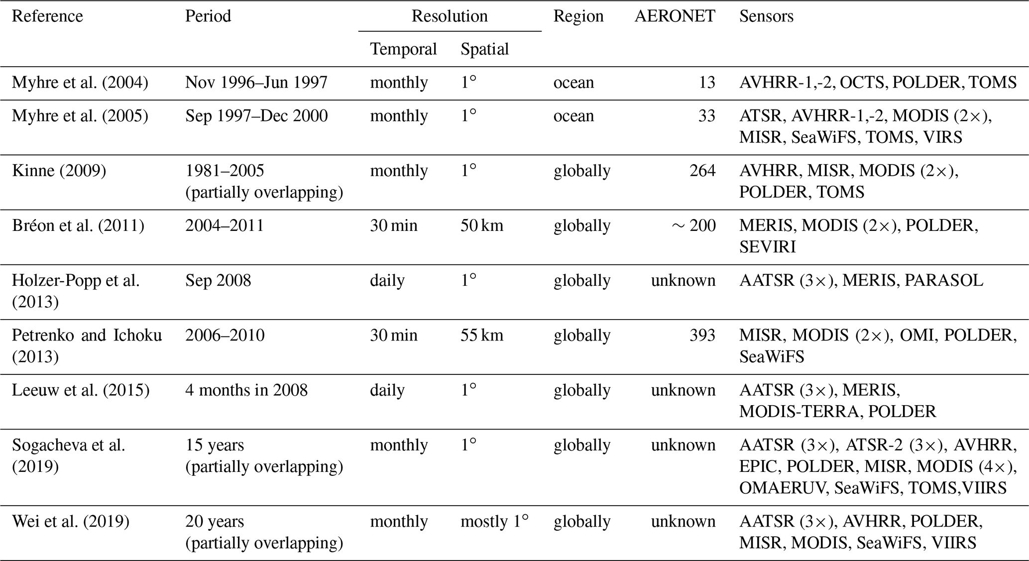

Table 1 Papers intercomparing multiple satellite datasets.

Most of the papers in Table 1 quantify only global biases for daily or monthly data. More than half of them use monthly satellite data, potentially introducing significant temporal representation errors (Schutgens et al., 2016b) in their analysis. Seldom is the spatial representativity of AErosol RObotic NETwork (AERONET) sites accounted for (Schutgens et al., 2016a), although most studies do exclude mountain sites. As a result both the evaluations with AERONET and the satellite product intercomparisons are no apples-to-apples comparisons. Finally, most studies do not systematically address (statistical or sampling) noise issues inherent in their analysis.

In this paper, we will assess spatially varying (as opposed to global) biases in multi-year averaged satellite AOD (appropriate for model evaluations). As truth references AERONET and Maritime Aerosol Network (MAN) data will be used. The analysis uses only AERONET sites with high spatial representativity and collocates all data within a few hours, greatly reducing representation errors. Throughout, a bootstrapping method is used to assess statistical noise in the analysis. Sampling issues (e.g. due the sparsity of AERONET sites) are addressed through, for example, a pair-wise satellite intercomparison.

This paper is the result of discussions in the AeroCom (AEROsol Comparisons between Observations and Models; https://aerocom.met.no, last access: 21 October 2020) and AeroSat (International Satellite Aerosol Science Network; https://aero-sat.org, last access: 21 October 2020) communities. Both are grassroots communities, the first organized around aerosol modellers and the second around retrieval groups. They meet every year to discuss common issues in the field of aerosol studies.

The structure of the paper is as follows. The remote sensing products are described in Sect. 2 and the methodology to collocate them in space and time in Sect. 3. Section 4 describes screening procedures for representative AERONET sites and establishes the robustness of our collocation procedure. Section 5 evaluates the satellite products individually against AERONET and MAN, at daily and multi-year timescales. An intercomparison of pairs of satellite products is presented in Sect. 6. A combined evaluation and intercomparison of the products is made in Sect. 7. More importantly, the diversity amongst satellite products is discussed and interpreted. A summary can be found in Sect. 8.

2 Remote sensing data

Original satellite L2 data were aggregated onto a regular spatio-temporal grid with spatio-temporal grid boxes of $\mathrm{1}{}^{\circ }\times \mathrm{1}{}^{\circ }\times \mathrm{30}$ min. The resulting super-observations ($\mathrm{1}{}^{\circ }\times \mathrm{1}{}^{\circ }\times \mathrm{30}$ min aggregates) are more representative of global model grid boxes (∼1^∘–3^∘ in size) while allowing accurate temporal collocation with other datasets. At the same time, the use of super-observations significantly reduces the amount of data without much loss of information (at the scale of global model grid boxes). A list of products used in this paper is given in Table 2. A colour legend for the different products can be found in Fig. 1. More explanation of the aggregation procedure can be found in Appendix A.

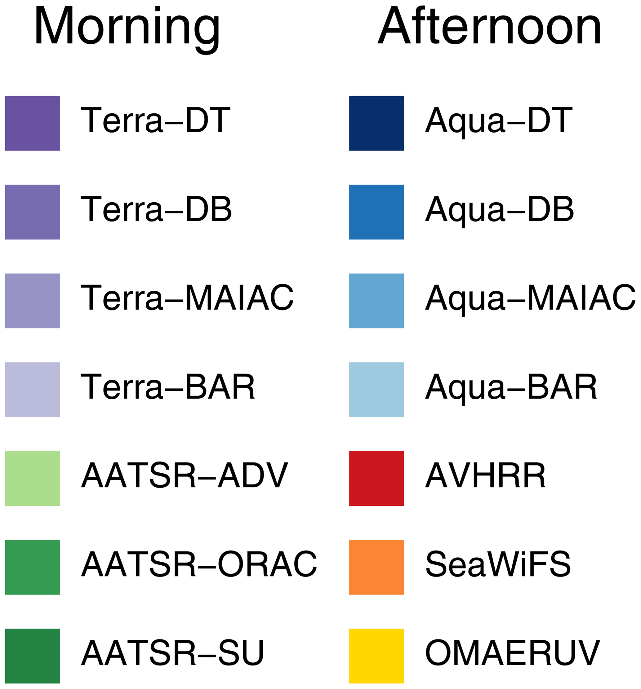
Figure 1 Colour legend used throughout this paper to designate the different satellite products, organized by approximate local Equator crossing time.

Remer et al. (2005)Hsu et al. (2013, 2019)Sayer et al. (2019)Lyapustin et al. (2018)Lipponen et al. (2018)Sogacheva et al. (2017)Thomas et al. (2009)North et al. (1999)North (2002)Bevan et al. (2012)Hsu et al. (2013)Sayer et al. (2012a, b)Hsu et al. (2017)Sayer et al. (2017)Ahn et al. (2014)Jethva et al. (2014)

Table 2 Remote sensing products used in this study.

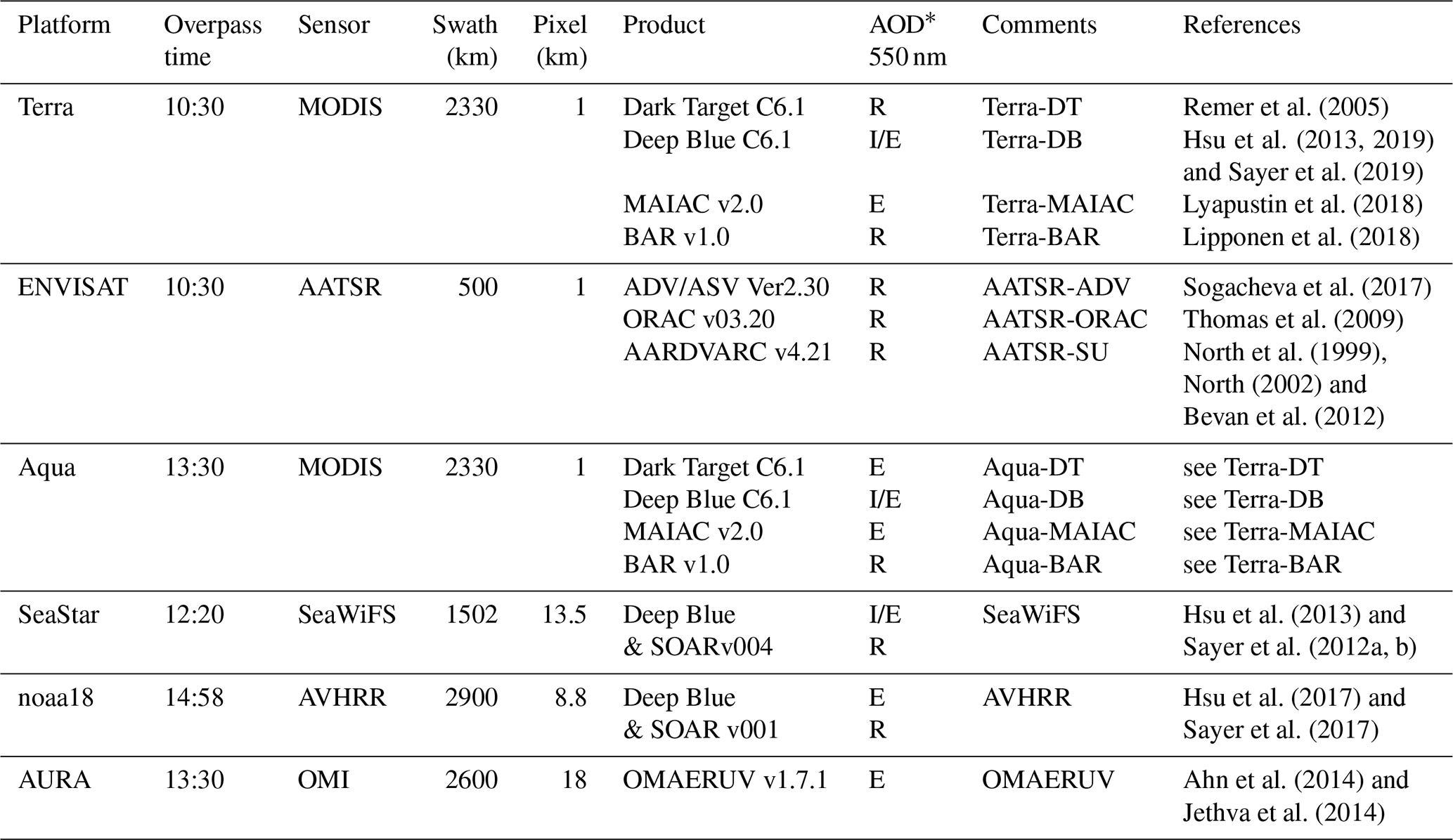
^* Interpolated or extrapolated to 550 nm, depending on surface type, or retrieved at 550 nm.

The main data are AOD at 550 nm, the wavelength at which models typically provide AOD. If AOD was not retrieved at this wavelength, it was interpolated (or extrapolated) from nearby wavelengths.

In addition, the number of L2 retrievals used per super-observation as well the average pixel size for these L2 retrievals were included. For some products (e.g. MODIS), this physical pixel size will vary as the view angle changes across the imager's field of view. In that case, actual pixel footprints can be difficult to calculate due to the Earth's curvature (Sayer, 2015), and only estimates were provided. Other products (MAIAC and those from AATSR) are based on regridded radiance data and use a fixed pixel size. The combination of number of retrievals and average pixel size can be used to estimate the spatial coverage: the fraction of a $\mathrm{1}{}^{\circ }\times \mathrm{1}{}^{\circ }$ grid box covered by L2 retrievals (at a particular time) per super-observation. This spatial coverage would ideally be 100 % but in practice is smaller for several reasons: the imager's field of view may miss part of the $\mathrm{1}{}^{\circ }\times \mathrm{1}{}^{\circ }$ grid box; sun glint, snow, desert surface or clouds may prevent retrievals; or retrievals may fail. As we use an estimate of coverage, based on an average pixel size, values in excess of 100 % do occur. We provide evidence in Sects. 5 and 6 that cloud masking is the dominant factor in determining spatial coverage; see also Zhao et al. (2013), who suggest that spatial coverage might be interpreted as an estimate of the complement to cloud fraction.

All products were provided globally for 3 years (2006, 2008 and 2010, years used in AeroCom control studies). Many products only provided data over land. Seven datasets belong to sensors that have an equatorial crossing time in the morning, and another seven belong to sensors that have an equatorial crossing time in the afternoon.

AERONET (Holben et al., 1998) DirectSun L2.0 V3 (Giles et al., 2019; Smirnov et al., 2000) and MAN L2.0 (Smirnov et al., 2011) data were downloaded from https://aeronet.gsfc.nasa.gov (last access: 19 May 2020). These AOD observations are based on direct transmission measurements of solar light and have a high accuracy of ±0.01 (Eck et al., 1999; Schmid et al., 1999). They were aggregated per site by averaging over 30 min. MAN aggregates were assigned averaged longitude and latitudes for those 30 min.

The entire satellite dataset requires 14 GB of storage and is stored in the netCDF format.

3 Collocation and analysis methodology

To evaluate and intercompare the remote sensing datasets, they will need to be collocated in time and space to reduce representation errors (Colarco et al., 2014; Schutgens et al., 2016b, 2017). In practice this collocation is another aggregation (performed for each dataset individually) to a spatio-temporal grid with slightly coarser temporal resolution (1 or 3 h; the spatial grid box size remains $\mathrm{1}{}^{\circ }\times \mathrm{1}{}^{\circ }$). This is followed by a masking operation that retains only aggregated data if they exist in the same grid boxes for all datasets involved. More details can be found in Appendix A.

During the evaluation of products with AERONET, a distinction will be made between either land or ocean grid boxes in the common grid. A high-resolution land mask was used to determine which $\mathrm{1}{}^{\circ }\times \mathrm{1}{}^{\circ }$ grid box contained at most 30 % land (designated an ocean box) or water (designated a land box). Most ocean boxes with AERONET observations will be in coastal regions, with some over isolated islands.

3.1 Taylor diagrams

A suitable graphic for displaying multiple datasets' correspondence with a reference dataset (“truth”) is provided by the Taylor diagram (Taylor, 2001). In this polar plot, each data point (r,ϕ) shows basic statistical metrics for an entire dataset. The distance from the origin (r) represents the internal variability (standard deviation) in the dataset. The angle ϕ through which the data point is rotated away from the horizontal axis represents the correlation with the reference dataset, which is conceptually located on the horizontal axis at radius 1 (i.e. every distance is normalized to the internal variability of the reference dataset). It can be shown (Taylor, 2001) that the distance between the point (r,ϕ) and this reference data point at (1,0) is a measure of the root mean square error (RMSE, unbiased). A line extending from the point (r,ϕ) is used to show the bias versus the reference dataset (positive for pointing clockwise).The distance from the end of this line to the reference data point is a measure of the root mean square difference (RMSD, no correction for bias).

3.2 Uncertainty analysis using bootstrapping

Our estimates of error metrics are inherently uncertain due to finite sampling. If the sampled error distribution is sufficiently similar to the underlying true error distribution, bootstrapping (Efron, 1979) can be used to assess uncertainties in, for example, biases or correlations due to finite sample size. Bootstrapping uses the sampled distribution to generate a large number of synthetic samples by random draws with replacement. For each of these synthetic samples, a bias (or other statistical properties) can be calculated, and the distribution of these biases provides measures of the uncertainty, e.g. a standard deviation, in the bias due to statistical noise. Bootstrapping has been shown to be reliable, even for relatively small sample sizes (that is the size of the original sample, not the number of bootstraps); see Chernick (2008). In this study, the uncertainty bars in some figures were generated by bootstrap analysis.

If the sampled error distribution is different from the true error distribution, bootstrapping will likely underestimate uncertainties. Sampled error distributions may be different from the true error distribution because the act of collocating satellite and AERONET data favours certain conditions; e.g. the effective combination of two cloud screening algorithms (one for the satellite product, the other for AERONET) may favour clear sky conditions and limit sampling of errors in case of cloud contamination. This uncertainty due to sampling is unfortunately hard to assess, but we attempt to address it by comparing evaluations for different combinations of collocated satellite products.

3.3 Error metrics for evaluation

For most of this study we will focus on the usual global error statistics (bias, RMSD, Pearson correlation, regression slopes), treating all data as independent. Regression slopes were calculated with a robust ordinary least squares regressor (OLS bisector from the IDL sixlin function; Isobe et al., 1990). This regressor is recommended when there is no proper understanding of the errors in the independent variable; see also Pitkänen et al. (2016). Global statistics may be dominated by a few sites with many collocations, which will skew results. We also performed analyses on regional scales, but they will not be shown. Instead we show as error metrics the bias (sign-less) and the correlation per site, averaged over all sites. These error metrics do not suffer from a few sites with many observations dominating the error statistics. Only sites with at least 32 collocations will be used in this last analysis.

4 Selection of AERONET sites and collocation criteria

Not all AERONET sites are equal. They differ in their spatial representativity for larger $\mathrm{1}{}^{\circ }\times \mathrm{1}{}^{\circ }$ areas and in their level of maintenance. Ideally, only sites with the highest spatial representativity and maintenance levels should be used for satellite evaluation. In addition, a temporal criterion for satellite collocation with AERONET observations needs to be established that yields sufficient data for analysis yet also allows meaningful comparison (i.e. the difference in observation times should not be too large).

Kinne et al. (2013) provide a subjective ranking of all sites (before 2009) based on their general level of maintenance and spatial representativity. The ranking is based on personal knowledge of the sites and is mostly qualitative. Schutgens (2019) provides an objective ranking for all sites (for all years) based on spatial representativity alone. This ranking is based on a high-resolution modelling study and is quantitative. While there is substantial overlap in their rankings for spatial representativity, there are also differences. Table 3 describes the AERONET site selections used in this paper.

Kinne et al. (2013)Schutgens (2019)

Table 3 AERONET site subsets.

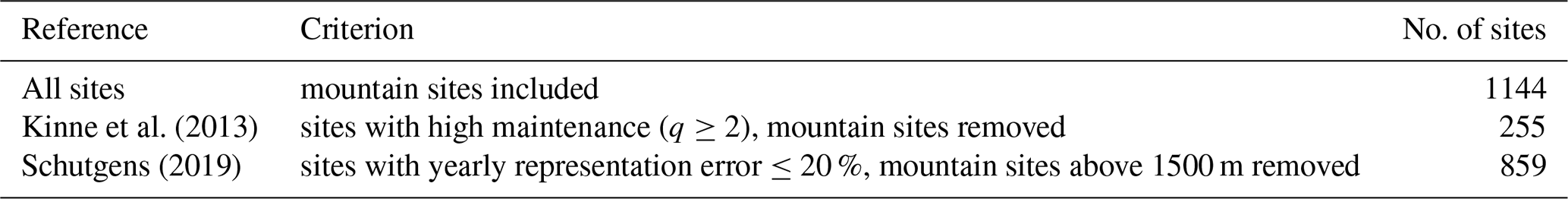
Kinne et al. (2013) only consider sites before 2009, with at least 5 months of data.

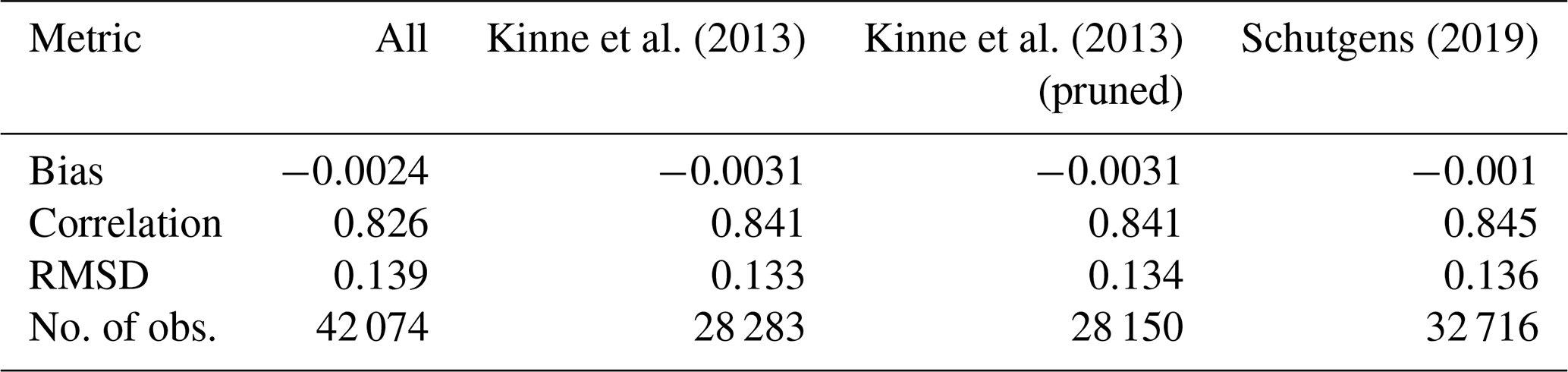
The impact of using a subset of AERONET sites like Kinne et al. (2013) or Schutgens (2019) (compared to the full dataset) on satellite product evaluation is to slightly increase correlations and decrease RMSDs; i.e. the satellite products compare better to AERONET data. As this occurs systematically for all products (see Fig. S1 in the Supplement), we believe these subsets contain AERONET sites substantially better suited for satellite evaluation. Averages for these metrics over all products are given in Table 4. As we later want to evaluate satellite products at individual sites, we will use the Kinne subset defined in Table 3 since it is based on both site representativity and maintenance level. Note, however, that the Schutgens subset allows for more observations for our study period, vastly more AERONET sites (including after 2009) and a slightly better comparison of the satellite products.

Kinne et al. (2013)Kinne et al. (2013)Schutgens (2019)

Table 4 Averaged product evaluation with AERONET depending on the selection of AERONET sites used as truth reference.

A further test of the AERONET sites subset consists of comparing them individually against all satellite products. It turns out there are four sites (Canberra, Crozet Island, Amsterdam Island and Tinga Tingana) that have low correlations with and/or high biases vs. all satellite products (see Fig. 2). While it is possible all satellite products fail badly for these four sites, we assume it is actually the sites that are, in a way not yet understood, poorly suited to satellite evaluation (e.g. representativity or maintenance issues not flagged up by Kinne et al., 2013). These four sites were excluded from our analysis (this only has a small impact on global statistics; see Table 4). Note that only for a minority of remaining sites (10 %) will all satellite products either overestimate or underestimate AOD. For most sites, the products form an ensemble of AOD values that straddle the AERONET value.

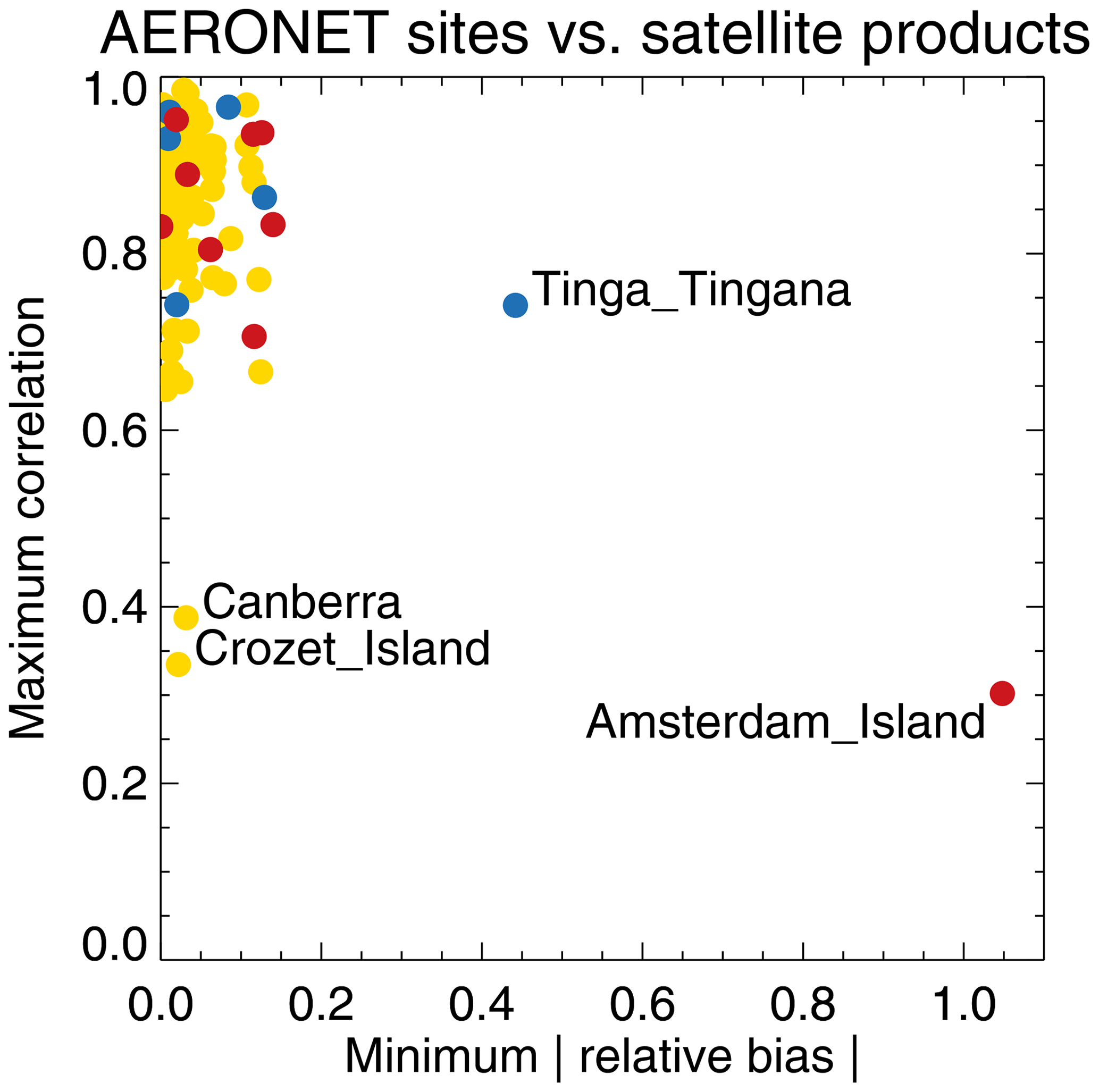
Figure 2 Minimum relative bias (sign-less) and maximum correlation per AERONET site, over all products. Red symbols indicate AERONET site bias is always positive; blue symbols indicate AERONET site bias is always negative. Yellow symbols indicate that site bias is positive versus some products and negative versus others. Products were individually collocated with AERONET (Kinne et al., 2013, selection) within 1 h.

Although we now have a subset of suitable AERONET sites for satellite evaluation, spatial representation errors still remain since a “point” observation (AERONET) will be used to evaluate satellite super-observations ($\mathrm{1}{}^{\circ }\times \mathrm{1}{}^{\circ }$ satellite aggregates). The difference between a satellite τ_s and AERONET τ_A super-observation AOD can be understood as the sum of observation errors in both products and a representation error ϵ_r:

$$\begin{array}{}\text{(1)}& {\mathit{\tau }}_{\mathrm{s}}-{\mathit{\tau }}_{\mathrm{A}}={\mathit{ϵ}}_{\mathrm{s}}+{\mathit{ϵ}}_{\mathrm{A}}+{\mathit{ϵ}}_{\mathrm{r}}.\end{array}$$

If we assume these errors are uncorrelated and have a Gaussian distribution, we can use the associated uncertainties (i.e. standard deviations of the errors) to determine the dominant contribution. AERONET observation uncertainty is estimated at σ_A=0.01 (Eck et al., 1999; Schmid et al., 1999), and representation uncertainty σ_r may be estimated as the standard deviation of L2 AOD retrievals over $\mathrm{1}{}^{\circ }\times \mathrm{1}{}^{\circ }$ (remember, the mean of those values is the super-observation itself). The latter assumes that satellite errors over a grid box are mostly constant. Since we also know the differences between satellite and AERONET data, satellite observational uncertainty σ_S can be estimated. This suggests that the satellite observational uncertainty is twice as large as the representation uncertainty (see also Fig. S2), confirming that it is reasonable to evaluate super-observations with AERONET point observations.

Table 5 Averaged product evaluation with AERONET depending on temporal constraints (pruned Kinne subset).

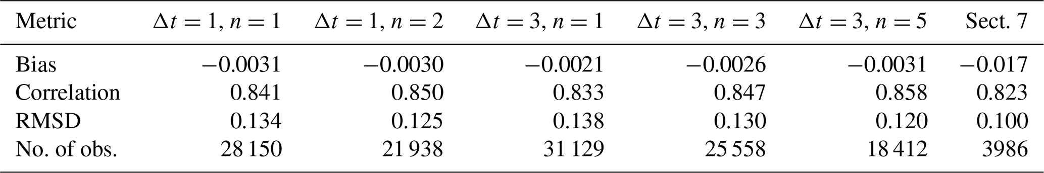
Lastly, we investigated the impact of the temporal collocation criterion Δt and minimum number of AERONET observations n on the satellite evaluation (it was 1 h in the previous analyses); see Table 5. It turns out that changing this number only has a small impact on evaluation metrics (see also Fig. S3) but quite a large impact on number of available observations. Given the substantial reduction in available collocated observations, we decided to require only a single AERONET super-observation for successful collocation.

We also considered the impact of these choices on regional evaluations. Broadly, similar conclusions can be drawn, although the analysis can become rather noisy due to smaller sample sizes.

5 Evaluation of individual satellite products

In this section we will evaluate individual satellite products with either AERONET or MAN observations. In both cases, the data were collocated within 1 h.

In Fig. 3 we see the evaluation with AERONET using Taylor diagrams (Taylor, 2001); see also Sect. 3.1. Over land the MODIS algorithms generally do very well, showing similar high correlations, although biases and standard deviations can be quite different. The same algorithm applied to either Aqua or Terra yields very similar results in the Taylor diagram. The exception is a relatively high bias for Terra-DT. The AATSR products generally have lower correlations than the MODIS products, although AATSR-ADV comes close. It is interesting to compare three products (Aqua-DB, SeaWiFS and AVHRR) that use a similar algorithm but with different amounts of spectral information. MODIS and SeaWiFS perform very similarly, but AVHRR shows much lower correlation. Some products globally overestimate AOD at the AERONET sites, whilst others underestimate it (see also Fig. 2). As the data count over land is high, statistical noise in these statistics is negligible, as can also be seen in Fig. S1, which is dominated by land sites.

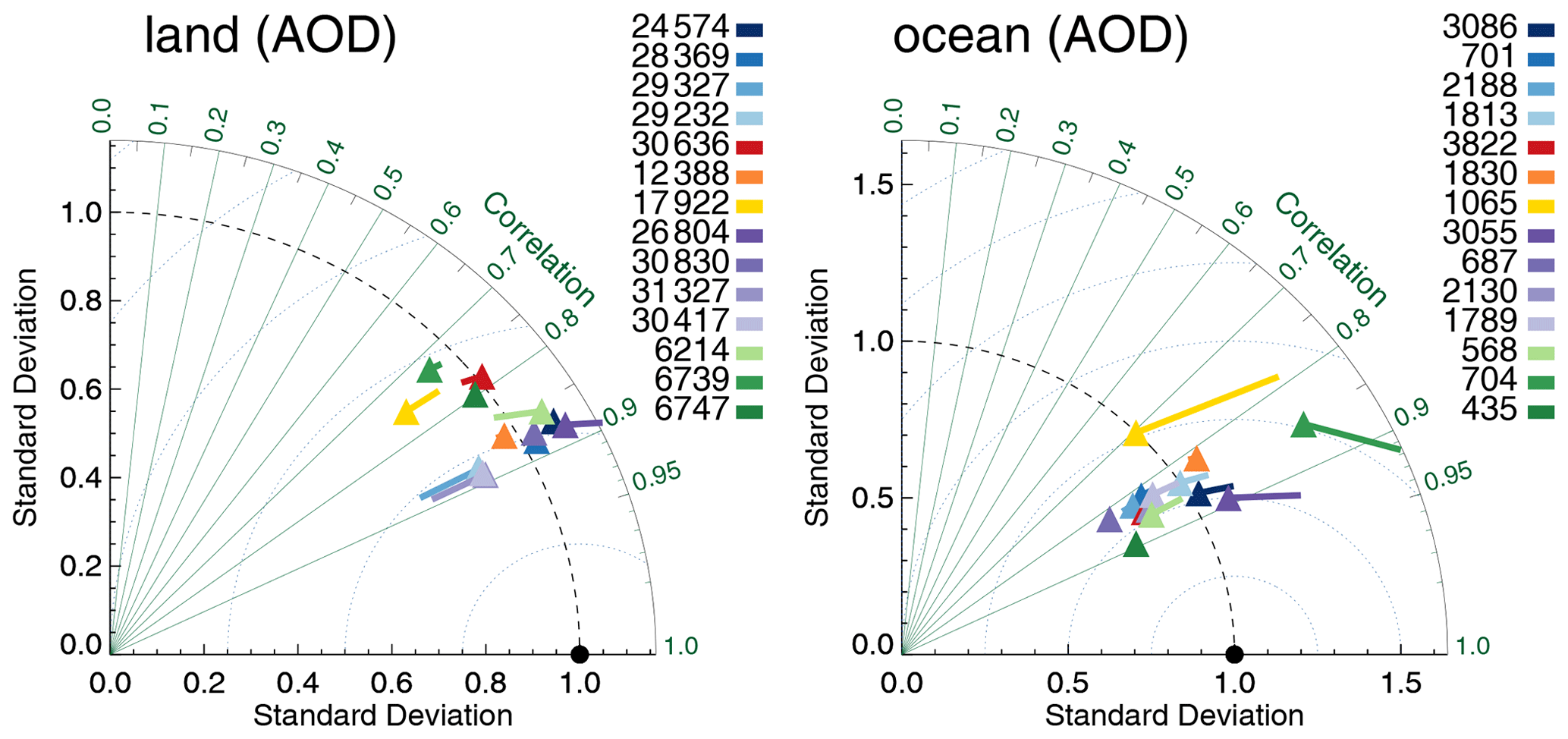
Figure 3 Taylor diagram for satellite products evaluated over either land or ocean with AERONET. Symbols indicate correlation and internal variability relative to AERONET; the line extending from the symbol indicates the (normalized) bias (see also Sect. 3.1). Colours indicate the satellite product (see also Fig. 1); numbers next to coloured blocks indicate the amount of collocated data. Products were individually collocated with AERONET (Kinne et al., 2013, selection, pruned) within 1 h.

Over ocean, the message is more mixed. The AATSR products do relatively better, while Terra/Aqua-DB seem to be slightly outperformed by AVHRR and SeaWiFS (note that Terra/Aqua-DB and BAR only retrieve data over land and the “over-ocean” analysis is confined to coastal regions). Over ocean no products significantly underestimate global AOD, although a few (e.g. SeaWiFS and Aqua-MAIAC) have small negative biases. Several products significantly overestimate global over-ocean AOD (e.g. Dark Target, OMAERUV and AATSR-ORAC). The data count for over-ocean evaluation is not very high, and consequently statistical noise in this analysis is larger than over land. A sensitivity study using bootstrapping (see Sect. 3.2) nevertheless suggests these results are quite robust. They are also partially supported by product evaluation with MAN in Fig. 4: the AATSR products do better than the other products, but it is clearly possible for the products to either over- or underestimate AOD globally. The data count for MAN evaluation is low, and statistical noise is large; see Fig. S4. For OMAERUV, for example, the uncertainty range suggests this could be either one of the worst- or best-performing products.

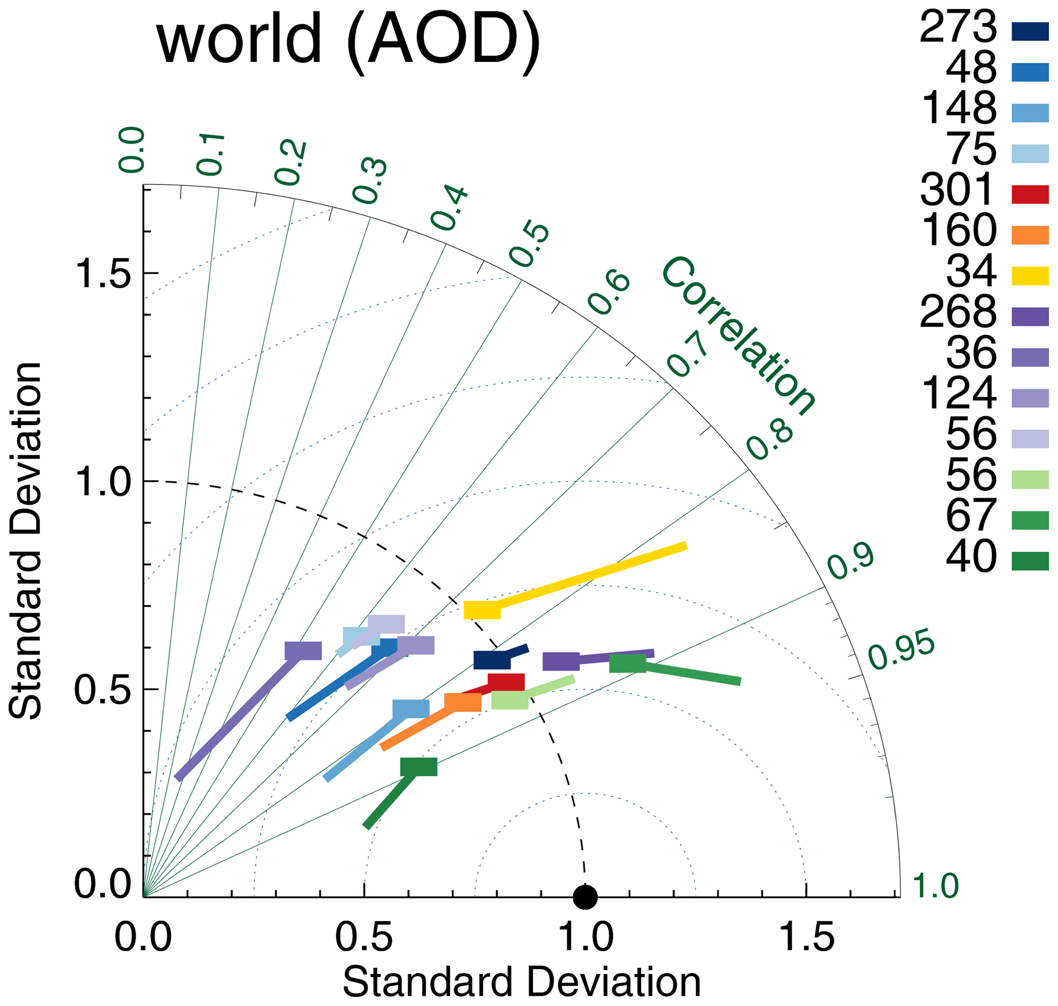
Figure 4 Taylor diagram for satellite products evaluated over either land or ocean with MAN. Symbols indicate correlation and internal variability relative to MAN; the line extending from the symbol indicates the (normalized) bias (see also Sect. 3.1). Colours indicate the satellite product (see also Fig. 1); numbers next to coloured blocks indicate the amount of collocated data. Products were individually collocated with AERONET (Kinne et al., 2013, selection, pruned) within 1 h.

If we split each product's data into two equally sized subsets depending on the collocated AERONET AOD (median AOD ∼0.12), it becomes obvious that the satellite products have much lower skill at low AOD; see Fig. 5. They correlate much worse with AERONET, show much higher internal variability than AERONET and exhibit relatively larger biases (normalized to AERONET's internal variability; see Sect. 3.1) than at high AOD. Note that biases at low AOD are all positive, while at high AOD they are negative (exception: Terra-DT).

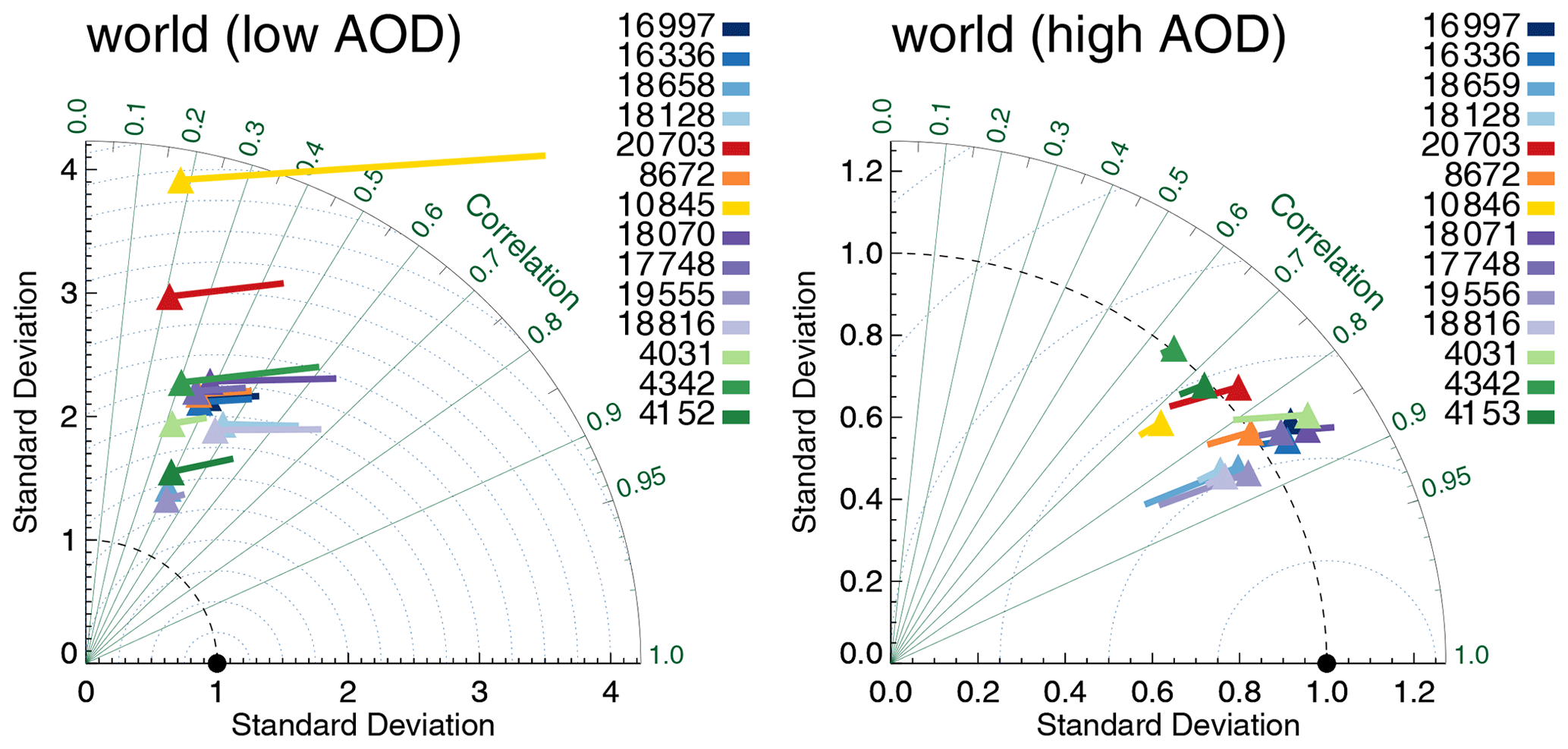
Figure 5 Taylor diagram for satellite products evaluated with AERONET at either low or high AOD (distinguished by median AERONET AOD ∼0.12). Symbols indicate correlation and internal variability relative to AERONET; the line extending from the symbol indicates the (normalized) bias (see also Sect. 3.1). Colours indicate the satellite product (see also Fig. 1); numbers next to coloured blocks indicate the amount of collocated data. Products were individually collocated with AERONET (Kinne et al., 2013, selection, pruned) within 1 h.

In Fig. 6, we consider the impact of spatial coverage on product evaluation. As minimum spatial coverage increases, the correlation with AERONET increases while the bias decreases. If spatial coverage is mostly determined by cloud screening, it seems reasonable that cloud contamination of AOD retrievals increases as spatial coverage decreases. This would lead to the observed behaviour of biases and correlations. In contrast, it is hard to use other factors determining spatial coverage (sun glint, surface albedo, failed retrievals) to explain this. We also note that the change with spatial coverage is quite dramatic for some products (AVHRR, OMAERUV, AATSR-ORAC), while for others it is rather small. It is expected that the quality of cloud masking (and hence the magnitude of cloud contamination) will differ among products (depending, for example, on pixel sizes or available spectral bands). It appears hard to determine a threshold value for spatial coverage beyond which there is no substantial change in all the metrics in the majority of products, so we continued to use all data.

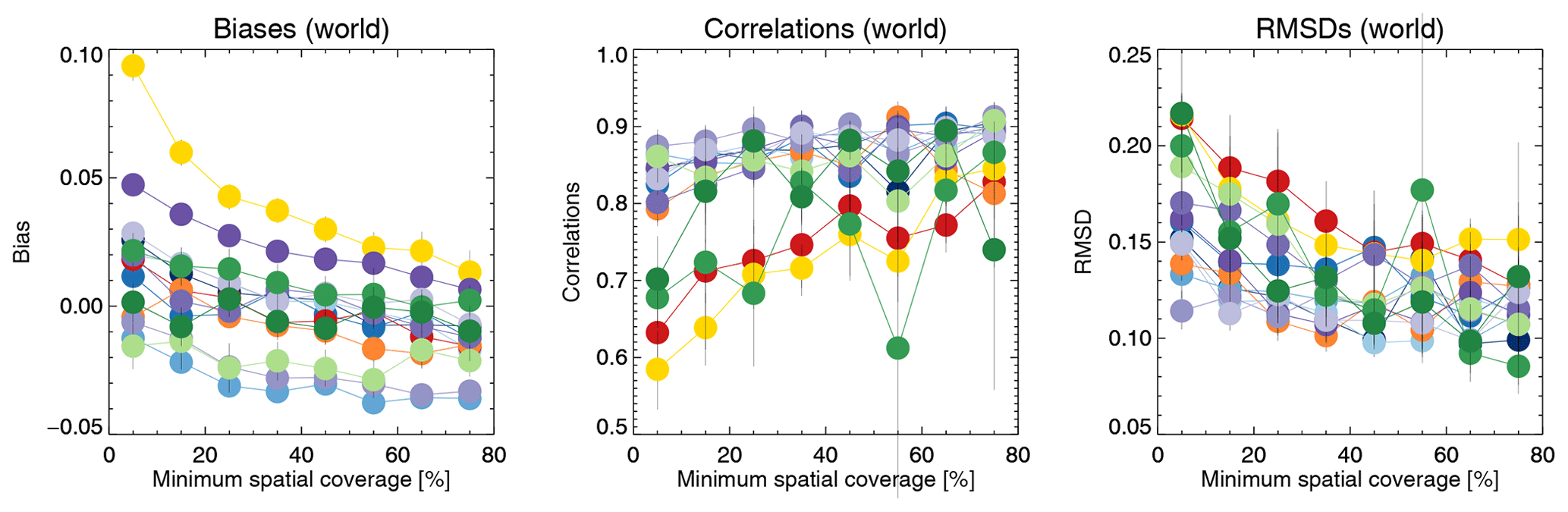
Figure 6 Evaluation of satellite products with AERONET, binned by minimum spatial coverage. Colours indicate the satellite product; see also Fig. 1. Individual collocation of datasets with AERONET (Kinne et al., 2013, selection, pruned) within 1 h. Error bars indicate the 5 %–95 % uncertainty range based on a bootstrap analysis of sample size 1000.

The impact of temporal averaging on product differences vs. AERONET is shown in Fig. 7. The “daily” graph shows differences for individual super-observations, while the “3-years” graph shows 3-year averages (averaged per site). Temporal averaging significantly reduces differences; e.g. the typical AVHRR difference decreases almost 3-fold from 0.077 to 0.027. In contrast, the typical difference for OMAERUV decreases only from 0.094 to 0.059, a factor of 1.6. It seems OMAERUV exhibits larger biases than AVHRR, which has rather large random differences. As noted before, the major part of the daily difference is due to observation errors, while a smaller part is due to representation errors. Previous analyses (Schutgens et al., 2016a, 2017; Schutgens, 2019) and our selection of AERONET sites suggest the 3-year average AOD difference will only have a small contribution from representation errors. After that amount of averaging, statistical analysis suggests that the typical 3-year differences may be interpreted as biases; i.e. the typical multi-year bias per site in Aqua-DT is 0.029. All products exhibit both positive and negative biases across AERONET. The global mean bias of a product (the big black dots in Fig. 7) is usually much smaller than the bias at any site and results from balancing errors across the network.

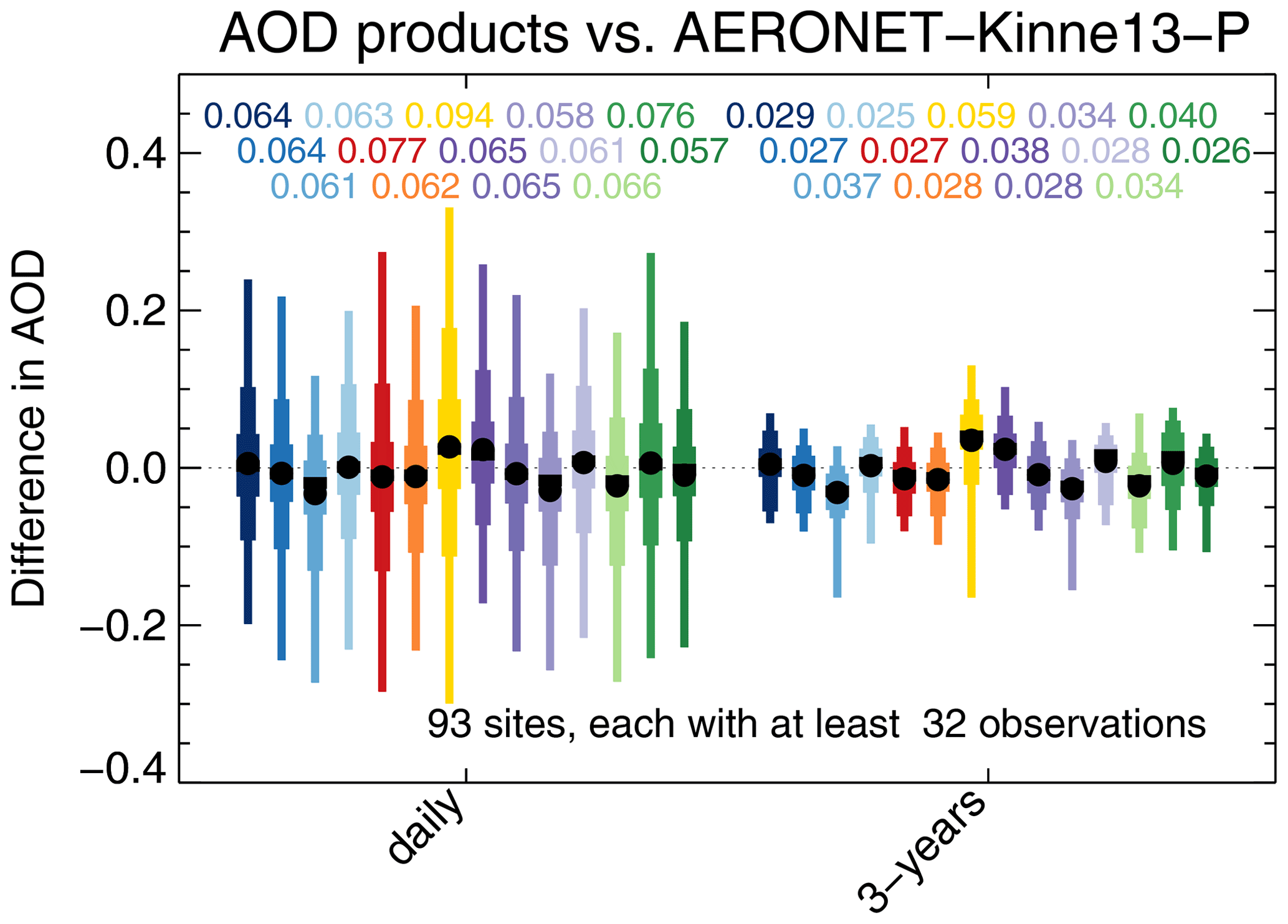
Figure 7 Evaluation of satellite products with AERONET, either for daily data or 3-year averages. The box-and-whisker plot shows 2 %, 9 %, 25 %, 75 %, 91 % and 98 % quantiles, as well as median (block) and mean (circle). Numbers above the whiskers indicate mean sign-less product errors. Colours indicate the satellite product; see also Fig. 1. Products were individually collocated with AERONET (Kinne et al., 2013, selection, pruned) within 1 h. All products use the same sites, each of which produced at least 32 collocations with each product.

Note that the Terra-DT bias is significantly larger than Aqua-DT's bias in Fig. 7. Levy et al. (2018) discuss a systematic difference between Terra and Aqua Dark Target AOD which they attributed to remaining retrieval issues.

Another way to evaluate the products is presented in Fig. 8, which shows the average correlation between any product and an AERONET site versus the average relative (sign-less) bias with an AERONET site. This analysis is different from the Taylor analysis presented earlier, where both correlation and bias were calculated across the entire dataset, instead of per site and then averaged across all sites. Figure 8 suggests that product biases per site are typically some 20 %. The relative performance of the products shows significant differences to the earlier Taylor analysis: AATSR-SU is now one of the top performers, while Terra/Aqua-DB show 1.3× larger biases than either Terra/Aqua-BAR or AATSR-SU (in the Taylor analysis, Terra/Aqua-DB have one of the smallest global biases).

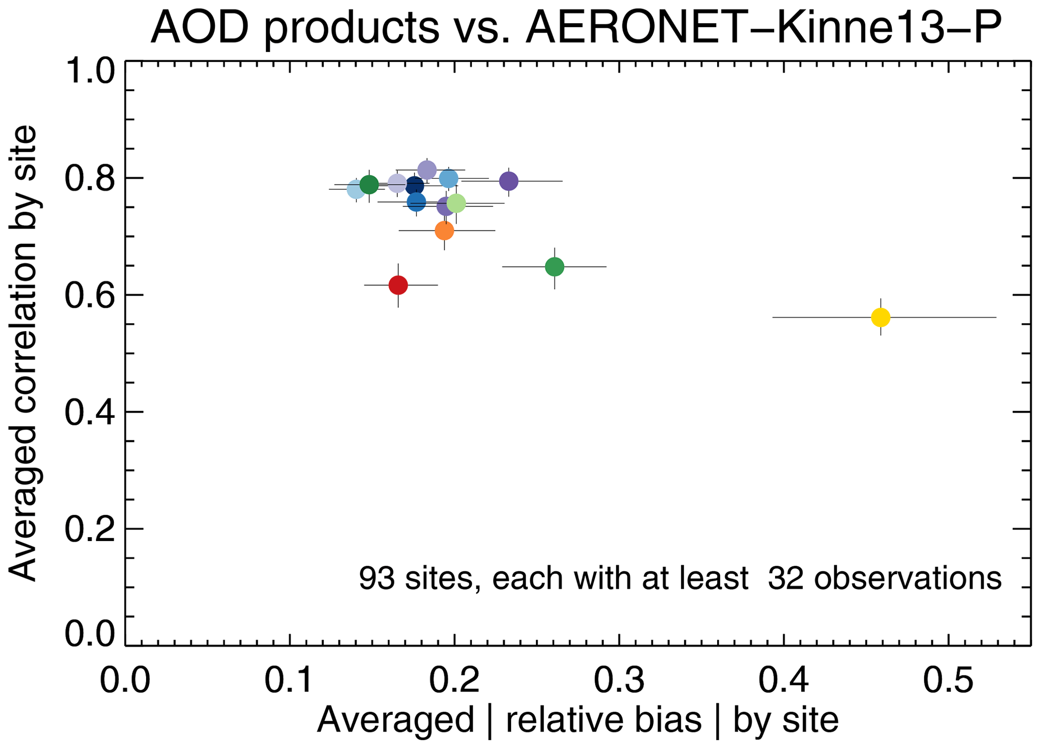
Figure 8 Evaluation of satellite products with AERONET per site, averaged over all sites. Error bars indicate the 5 %–95 % uncertainty range based on a bootstrap analysis of sample size 1000. Colours indicate the satellite product; see also Fig. 1. Products were individually collocated with AERONET (Kinne et al., 2013, selection, pruned) within 1 h. All products use the same sites, each of which produced at least 32 collocations with each product.

Both in Figs. 7 and 8, we have considered only AERONET sites that provide a minimum of 32 collocated observations. Although each product was individually collocated with AERONET, only those sites that are common across all product collocations were retained for analysis.

A more detailed look at each product and its evaluation against AERONET is provided in Figs. 9, 10, 11 and 12. The following are shown: a scatterplot of (daily) collocated super-observations vs. AERONET; the impact of spatial coverage on the difference between satellite and AERONET AOD; a global map of the 3-year averaged product AOD; and a global map of the difference of the 3-year averaged product AOD with AERONET (again, using only sites with 32 or more collocations).

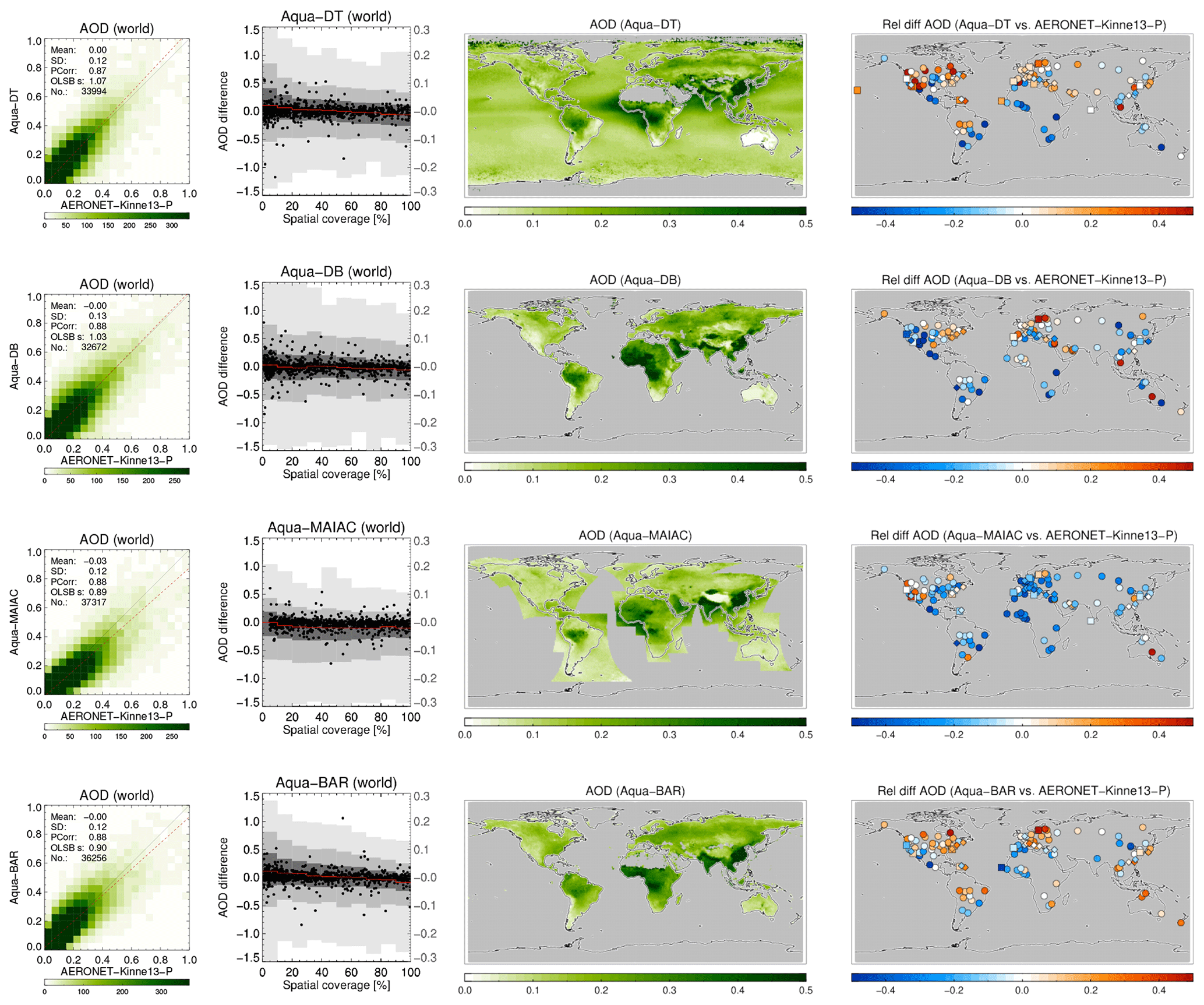
Figure 9 For MODIS-Aqua products the following are shown: a scatterplot of individual super-observations versus AERONET (mean and standard deviation refer to the difference with AERONET; PCorr and OLSB refer to the linear correlation and a robust least squares estimator of the regression slope); the AOD difference for individual super-observations as a function of spatial coverage (individual data, subsampled to a 1000 points, are shown as black dots using the left-hand axis, while the distribution per coverage bin, in greyscale, indicating 2 %, 9 %, 25 %, 75 %, 91 % and 98 % quantiles, uses the right-hand axis); a global map of the 3-year AOD average; and a global map of the 3-year AOD difference average with AERONET (if site provided at least 32 observations; land sites are circles, ocean sites are squares, the remainder are diamonds). Products were individually collocated with AERONET (Kinne et al., 2013, selection, pruned) within 1 h.

Figure 10 Same as Fig. 9, for AVHRR, SeaWiFS and OMAERUV products.

Figure 11 Same as Fig. 9, for MODIS-Terra products.

Figure 12 Same as Fig. 9, for AATSR products.

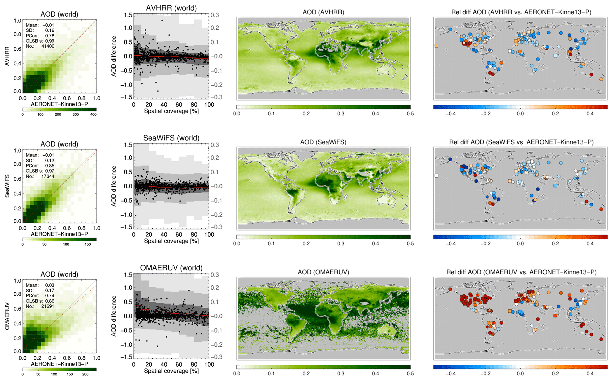
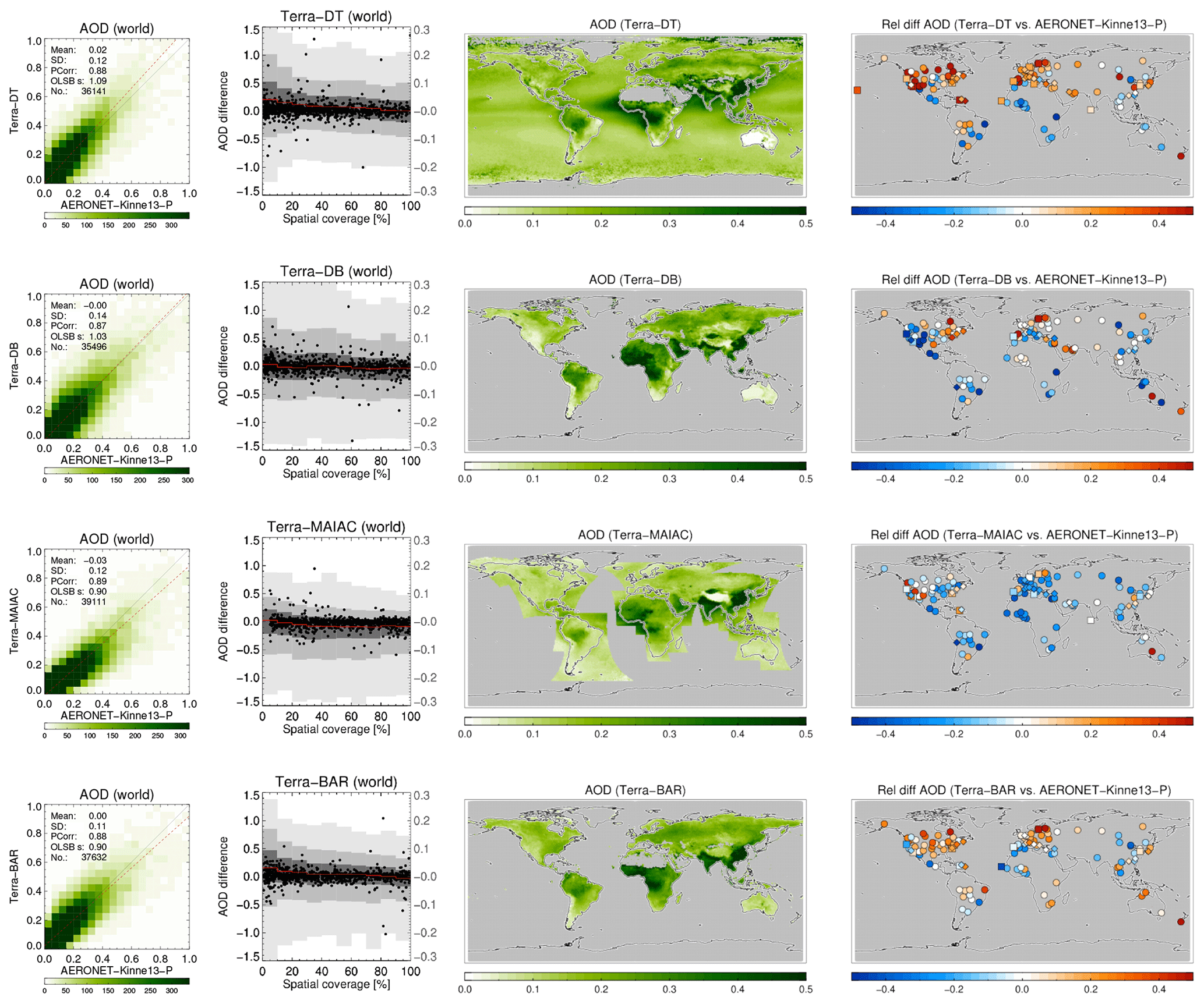
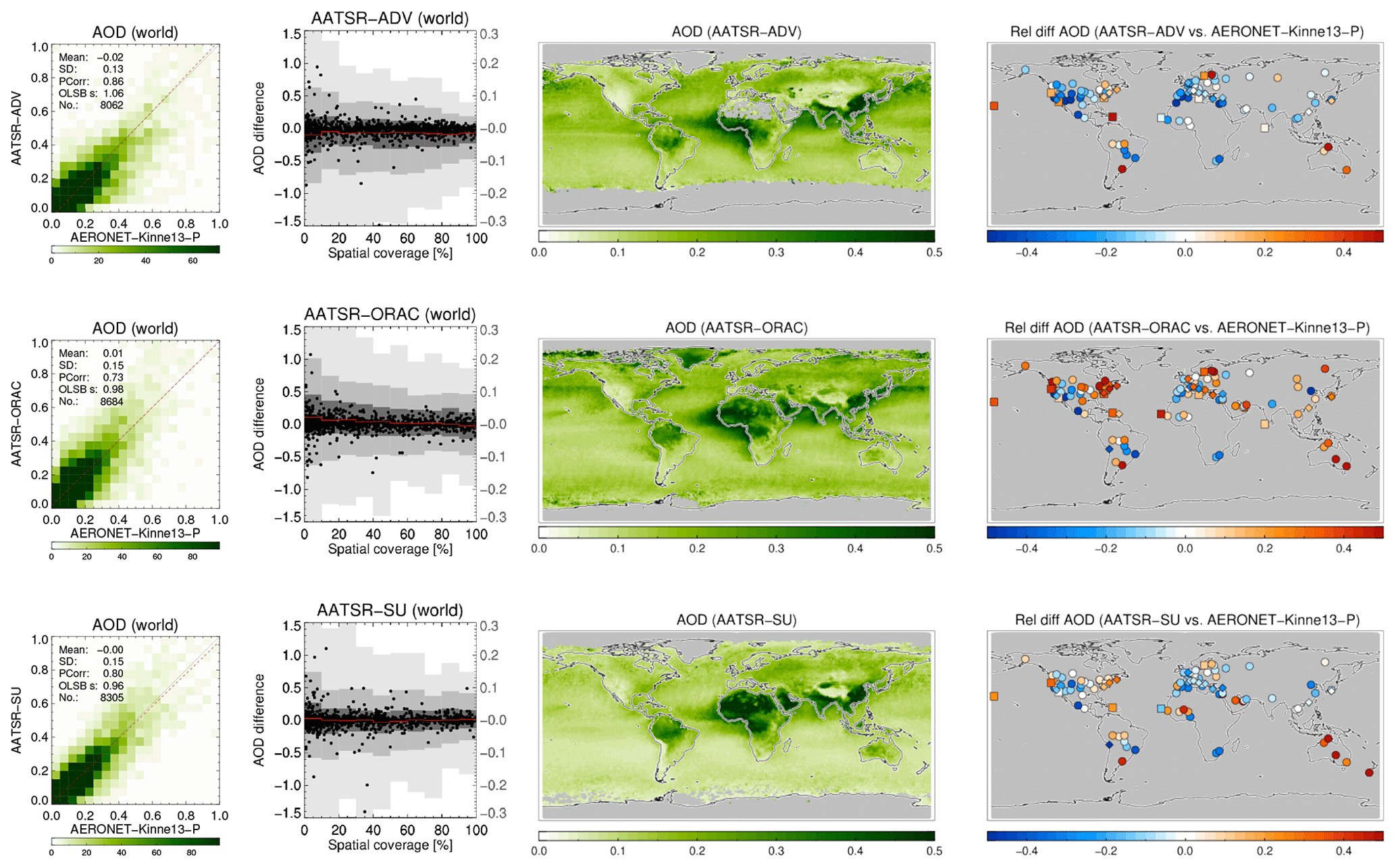
The scatterplots typically show good agreement with AERONET: correlations vary from 0.73 to 0.89, with regression slopes of 0.99 possible (mean and standard deviation refer to the difference with AERONET). The impact of spatial coverage on the differences with AERONET is consistent for all products and relatively muted, as also seen in the right panel of Fig. 6. The global maps of AOD show first of all the extent of the product: Terra/Aqua-DB, MAIAC and BAR provide no significant coverage of the oceans, while OMAERUV mostly seems to cover the large outflows over ocean. Unlike its most recent version, the MAIAC product used in this study misses a sizable portion of Siberia. Terra/Aqua-DT & BAR, AATSR-ADV and, to a lesser degree, AVHRR do not retrieve data over the desert regions in northern Africa and the Middle East. Terra/Aqua-DT, by the way, sometimes produces negative AOD, leading to, for example, very low values for averaged AOD over Australia. (The Dark Target algorithm can retrieve negative AOD values, for example, as a result of overestimating surface albedo, and the Dark Target team retains those values to prevent skewing the whole dataset to larger values.) In the global maps of 3-year averaged differences with AERONET, land sites are shown by circles, ocean sites by squares and the remainder by diamonds. These maps show distinct spatial patterns: for example, Aqua-DT mostly overestimates AOD in the Northern Hemisphere and underestimates it in the Southern Hemisphere; OMEARUV overestimates AOD everywhere except in the African greenbelt and south-east Asia; and MAIAC mostly underestimates AOD (MAIAC MODIS C6 lacks seasonal dependence of aerosol models, which leads to an underestimation during the biomass burning or dust seasons with high AOD. This will be corrected in C6.1). Regional patterns can also be seen; e.g. several products overestimate AOD in the eastern continental United States and underestimate it in the west.

6 Pair-wise intercomparison of the satellite datasets

In this section, we will intercompare the various satellite products by collocating them pair-wise within 1 h. Our analysis will be split between products for either morning or afternoon platforms as this usually leads to a large amount of collocated data with an almost global distribution. However, even products from, for example, Terra and Aqua can be collocated (at high northern latitudes) and will be discussed as well.

The difference in 3-yearly AOD is shown in Figs. 13 and 14 for morning and afternoon satellites, respectively. We see that the majority of collocated products only provides data over land. AOD differences behave very smoothly over ocean but show a lot of spatial variation over land. AOD differences can be significant and exceed 50 %. Over ocean, the difference is longitudinally fairly homogenous, with a clear latitudinal dependence. Over land, regional variability often tracks land features: the Rocky Mountains, the Andes, the Sahara and the African greenbelt can all be easily identified. That suggests albedo estimates as a driver of product difference. What is remarkable is the relatively large spatial scale involved. This analysis confirms the one in the previous section in which spatial patterns in AOD bias against AERONET were discussed and extends it in more detail. The contrasts in the differences over land and neighbouring ocean (e.g. African outflow for Terra-DT with AATSR-SU or AATSR-ADV, or Aqua-DT with OMAERUV, or AVHRR with SeaWiFS) may likewise be driven by the albedo estimate. The OMAERUV product consistently estimates higher AOD than all other products, with the possible exception of areas with known absorbing aerosol.

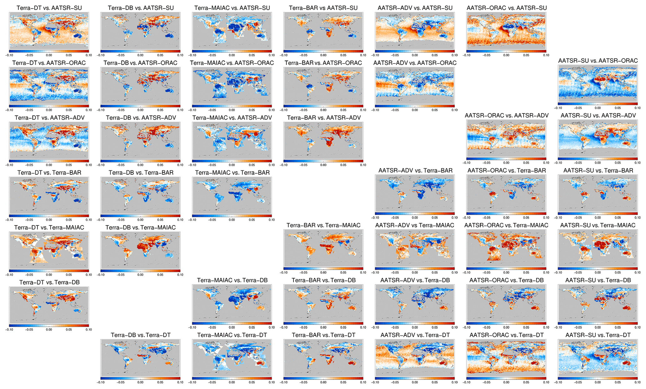
Figure 13 Global maps of the 3-year averaged difference in AOD for satellite products on morning satellites. Products were collocated pair-wise within 1 h.

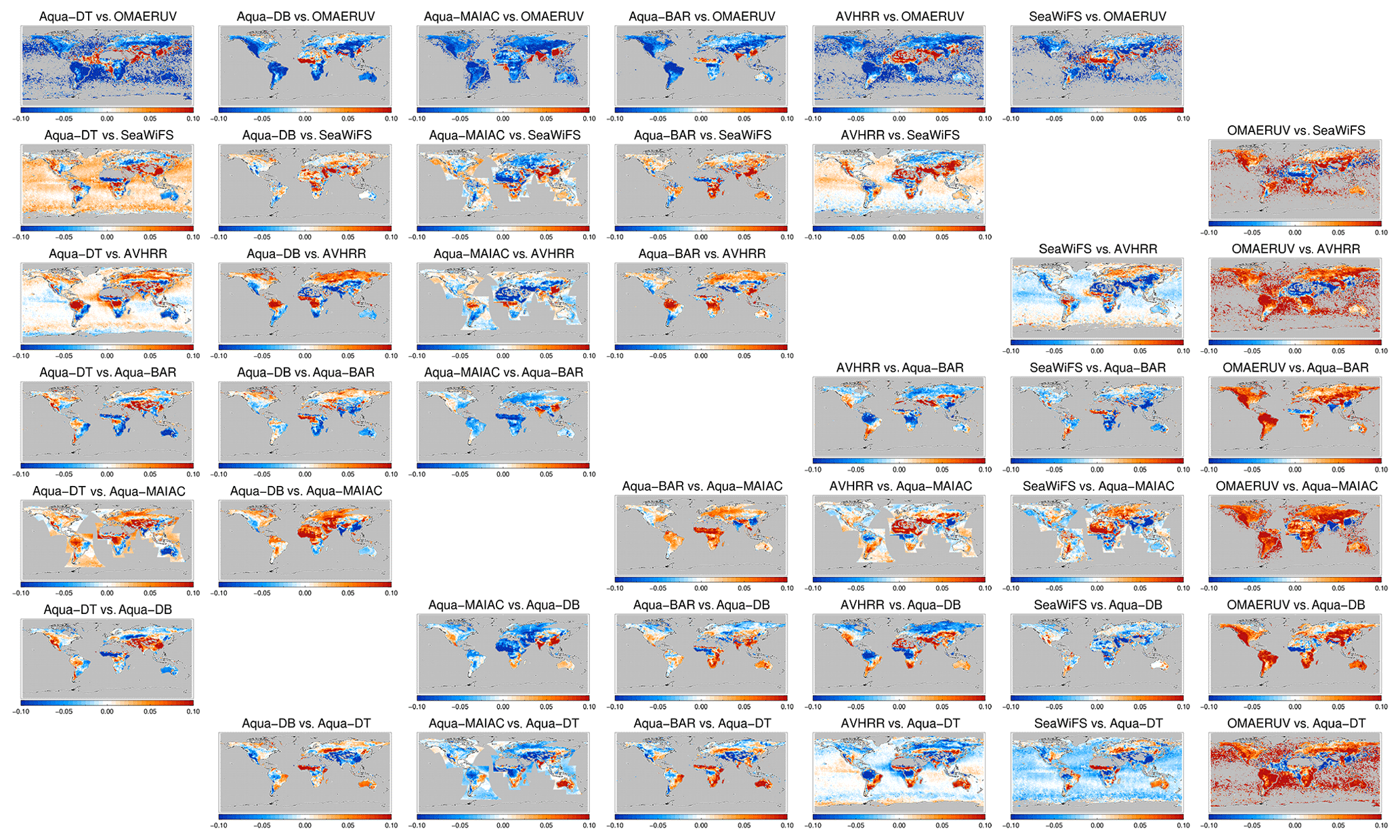
Figure 14 Global maps of the 3-year averaged difference in AOD for satellite products on afternoon satellites. Products were collocated pair-wise within 1 h.

Products retrieved using the same retrieval scheme but observations from different platforms can be intercompared as well (MODIS on Aqua and Terra). Collocations are now limited to a fairly narrow latitudinal belt near the North Pole; see Fig. 15. The differences in AOD appear much more muted, suggesting that algorithms are the major driver of product difference, not differences in orbital overpass times or issues with sensor calibration. This is further supported by the difference amongst, for example, AATSR products, which employ different algorithms but the same measurements (Fig. 13). The three products based on the Deep Blue algorithm (Aqua-DB, AVHRR and SeaWiFS) suggest that already small algorithmic differences (due to different spectral bands) can yield significant differences.

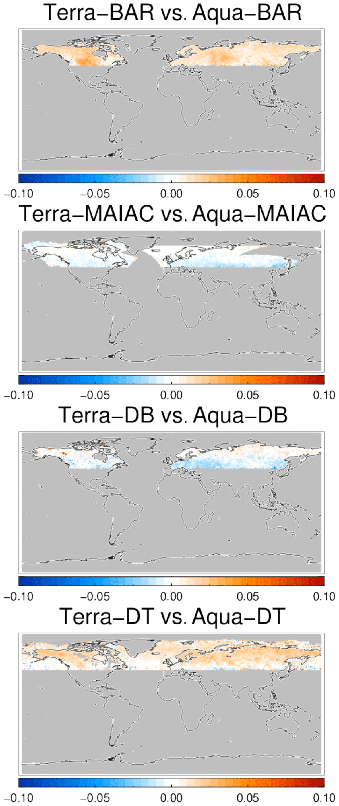
Figure 15 Global maps of the 3-year averaged difference in AOD for products based on the same algorithm and either Aqua and Terra satellites. Products were collocated pair-wise within 1 h.

In addition to 3-year biases, correlations of collocated pairs of AOD super-observations were also considered; see Fig. 16. The products derived from Aqua and Terra MODIS measurements tend to correlate well, with lesser correlation amongst the AATSR products. The highest correlation is found for products using the same algorithm and a similar sensor but a different platform (Terra/Aqua). The very low correlations for AATSR-ORAC with Aqua products stand out, but no explanation was found. Here again only collocations over high northern latitudes are available. Figure 16 also shows correlations for spatial coverage for all collocated product pairs. These turn out to be quite low. Even though the products apparently identify different parts of a $\mathrm{1}{}^{\circ }\times \mathrm{1}{}^{\circ }$ grid box as being suitable for aerosol retrieval, they still agree quite well on aggregated AOD.

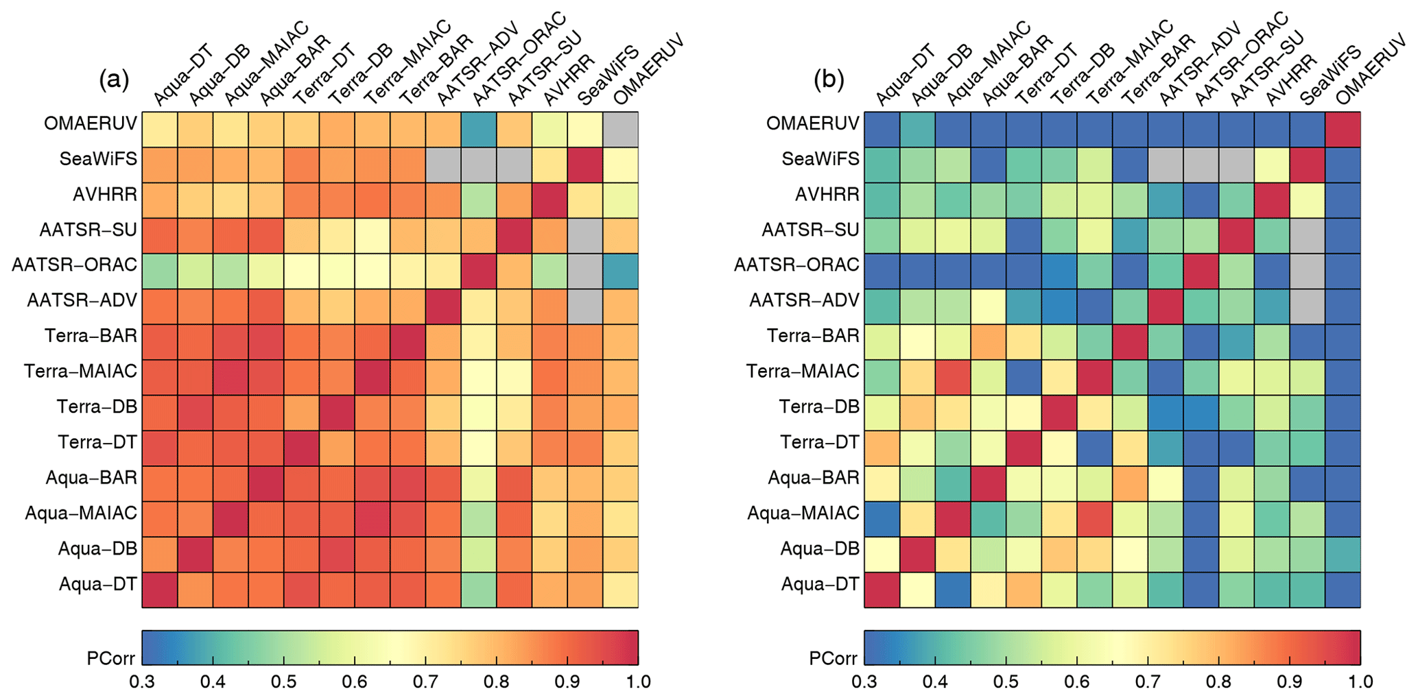
Figure 16 (a) Correlation of AOD super-observations for satellite products. (b) Correlation of spatial coverage in super-observations for satellite products. Products were collocated pair-wise within 1 h.

Figure 17 shows scatterplots of AOD and spatial coverage for selected collocated products. It is obvious that the agreement in AOD is far greater than the agreement in spatial coverage. Only when we consider collocated products for the same algorithm from different satellites can remarkable agreement be found (e.g. Terra/Aqua MAIAC). For different products using the same sensor, spatial coverage can differ greatly, even though the observed scene is the same.

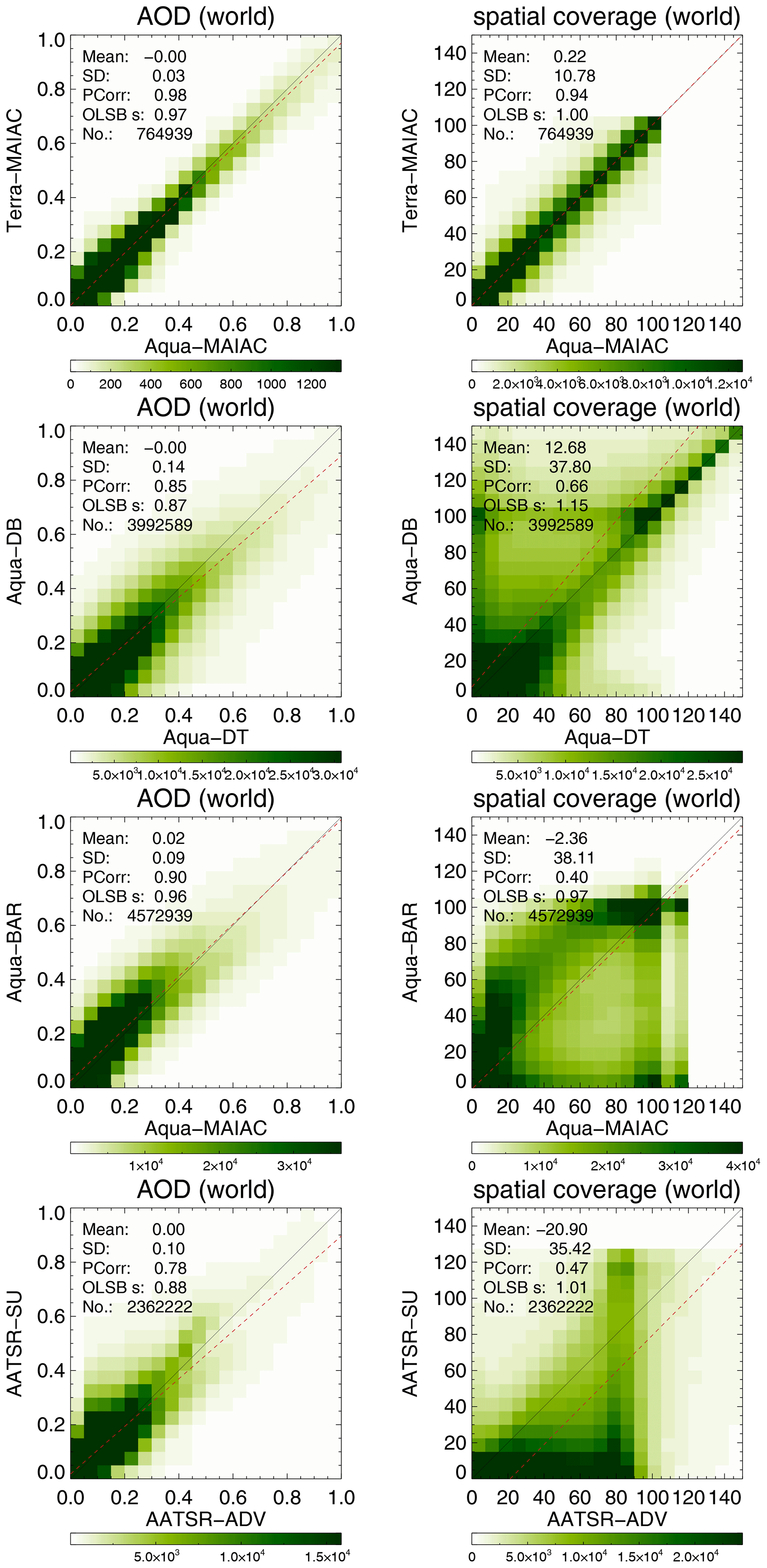
Figure 17 Scatterplot of AOD and spatial coverage from super-observations for selected satellite products. Products were collocated pair-wise within 1 h.

As with AERONET evaluation, product differences depend on spatial coverage; see Fig. S5. AOD agrees better when the spatial coverage is high, and this is more pronounced in the wings of the difference distributions (“outliers”). Fortunately, the impact on AOD differences is not that large: Fig. 18 shows the ratio of mean sign-less difference in AOD for spatial coverages of 90 %–100 % to 0 %–10 %. Typically this ratio is a factor of 0.57. The simplest explanation for the impact of spatial coverage on product differences is that this coverage is the complement to cloud fraction, and low coverage equals high cloud fraction. Associated cloud contamination can then explain the larger differences at low coverage. In other words, at very low spatial coverage, ∼40 % of the difference may be due to cloud contamination (see also Fig. S6, which shows impact of coverage). A similar weak dependence on AOD evaluation is seen in Figs. 9, 10, 11 and 12. One possible explanation is that aggregation into super-observations has a beneficial impact by tempering retrieval errors from cloud contamination.

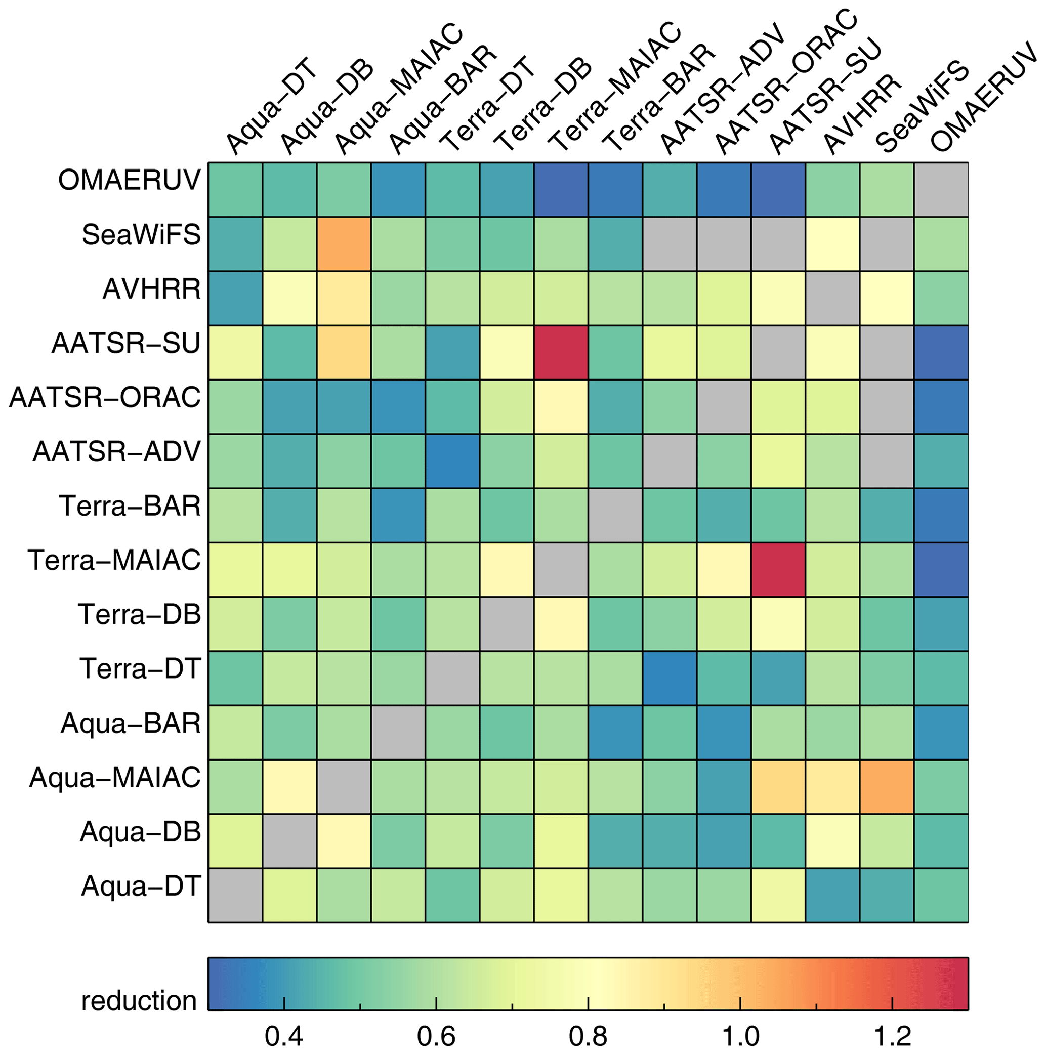
Figure 18 The ratio of typical difference (mean of sign-less difference) for spatial coverage at 90 %–100 % to 0 %–10 %. Products were collocated pair-wise within 1 h.

7 Intercomparison and evaluation of collocated morning or afternoon products

In this section, we will perform an apples-to-apples comparison of the satellite products, collocating either all morning or all afternoon products together. To ensure sufficient numbers of collocated data, the temporal collocation criterion was widened to 3 h. Even so, a significant reduction in data amount results from collocating so many datasets. If we include AERONET in the collocation, the total count will go down from ∼ 28 000 to about 4000 collocated cases.

The resulting Taylor diagram is shown in Fig. 19 and can be compared to Fig. 3. The Terra products show reduced correlation, now almost on par with the AATSR products. The Aqua and Terra products are not collocated together and, in contrast to Fig. 3, are clearly separated in the Taylor diagram. Also, the majority of datasets have negative biases with respect to AERONET. A more in-depth comparison is shown in Fig. 20. RMSD shows the most conspicuous changes: across the board RMSDs for the simultaneous collocation of seven satellite products with AERONET are much smaller. Global biases are shifted towards negative values; for example, OMAERUV now has a much smaller bias, while Aqua-DT has a much larger negative bias. Correlations are unaffected, except for the Terra and the AATSR-SU products. In all cases, the uncertainty ranges suggest that the differences are statistically significant.

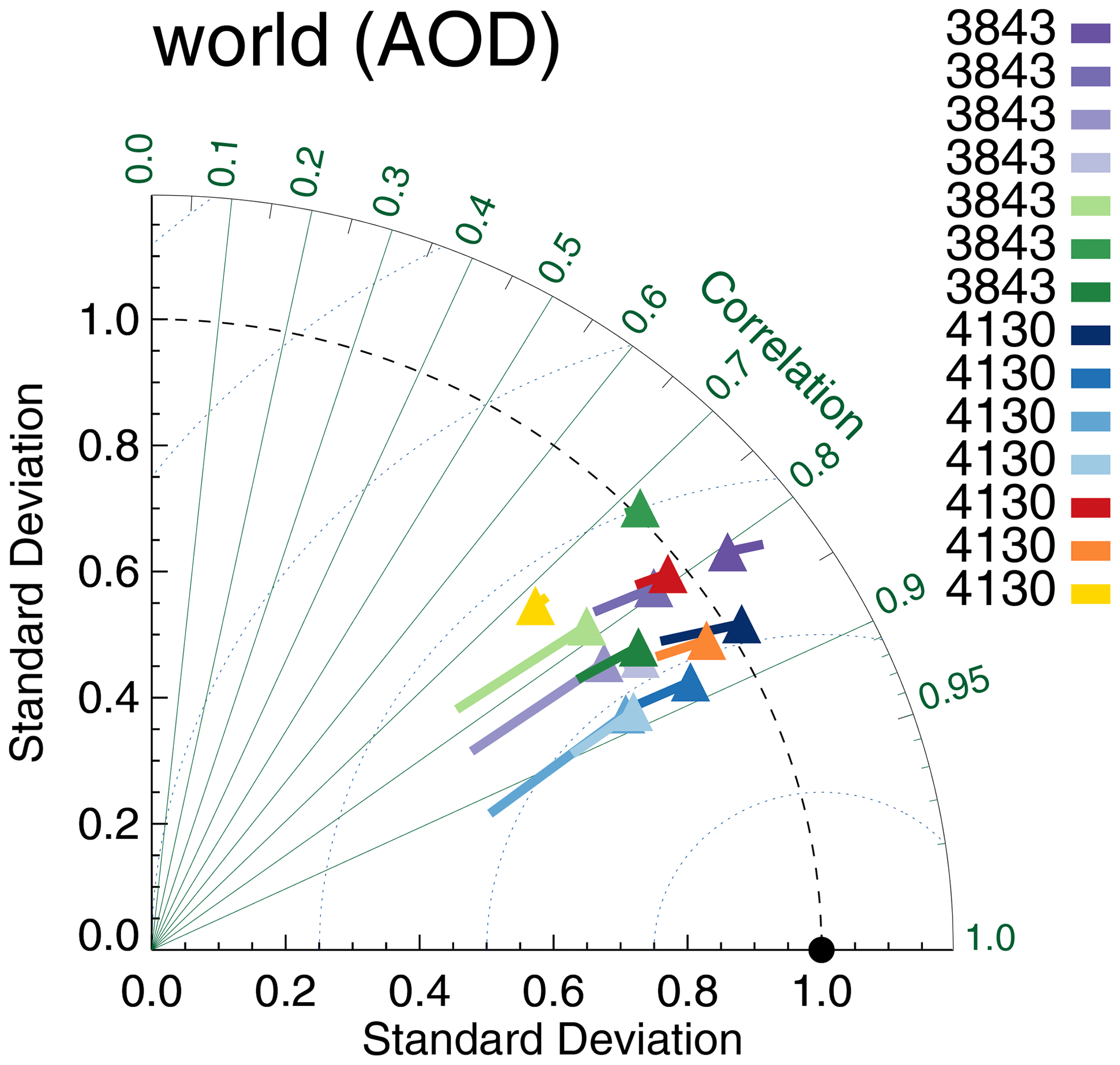
Figure 19 Taylor diagram for satellite products evaluated with AERONET. Symbols indicate correlation and internal variability relative to AERONET; the line extending from the symbol indicates the (normalized) bias (see also Sect. 3.1). Colours indicate the satellite product (see also Fig. 1); numbers next to coloured blocks indicate the amount of collocated data. All morning products were collocated together with AERONET (Kinne et al., 2013, selection, pruned) within 3 h, similar for all afternoon products.

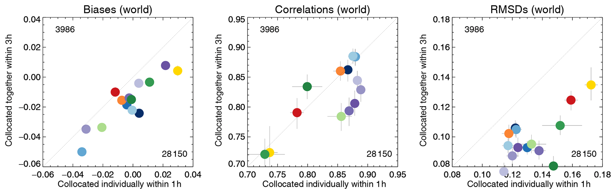
Figure 20 Comparison of the evaluation of satellite products for different dataset collocations. Horizontal axis: individual collocation with AERONET (within 1 h). Vertical axis: combined collocation of morning or afternoon products with AERONET (within 3 h). Colours indicate the satellite product; see also Fig. 1. Numbers in the upper left and lower right corner indicate the amount of collocated data, averaged over all products. The AERONET data are the Kinne et al., 2013, selection, pruned. Error bars indicate the 5 %–95 % uncertainty range, based on a bootstrap sample of 1000.

Both evaluations in Fig. 20 are valid in their own right. The evaluation of individual products with AERONET yields large amounts of data, while the simultaneous collocation of multiple morning or afternoon products allows proper intercomparison, without the added uncertainty due to different spatio-temporal sampling. Depending on one's point of view, it is possible to say that either results are not very different (considering all products, the relative performance of datasets does not change much) or quite different (considering the best-performing products, significant changes are visible).

The simultaneous collocation of multiple products yields a subset of the collocated data that were studied in Sect. 5, although for every product the subset from the “original” is different. Unfortunately, we have not been able to explain the different evaluation results. Due to the different collocation criteria, there are differences in the mean spatial coverage of the super-observations and in the relative number of collocations per AERONET site and per year. How this affects each product differs, and no systematic variation was found to help explain results. Ultimately this is testament to the complex influence of observational sampling.

Collocating either the morning or afternoon products without AERONET allows us to study diversity between these datasets on a global scale. Relative diversity is defined here as the relative spread (standard deviation divided by mean) calculated at each grid box from the 3-year averaged AOD of seven (collocated) products; see Fig. 21. Here we have used all seven morning or afternoon products over most of the land. Over ocean, the major desert regions and Siberia, not all products provided data, and only a subset was used. Over ocean, only Terra-DT and the three AATSR products or Aqua-DT, AVHRR and SeaWiFS were used. Over the desert regions (outlined in blue), only Terra-DB, Terra-MAIAC, AATSR-ORAC and AATSR-SU or Aqua-DB, Aqua-MAIAC, SeaWiFS and OMAERUV were used. Over Siberia (outlined in blue), no data were present for MAIAC.

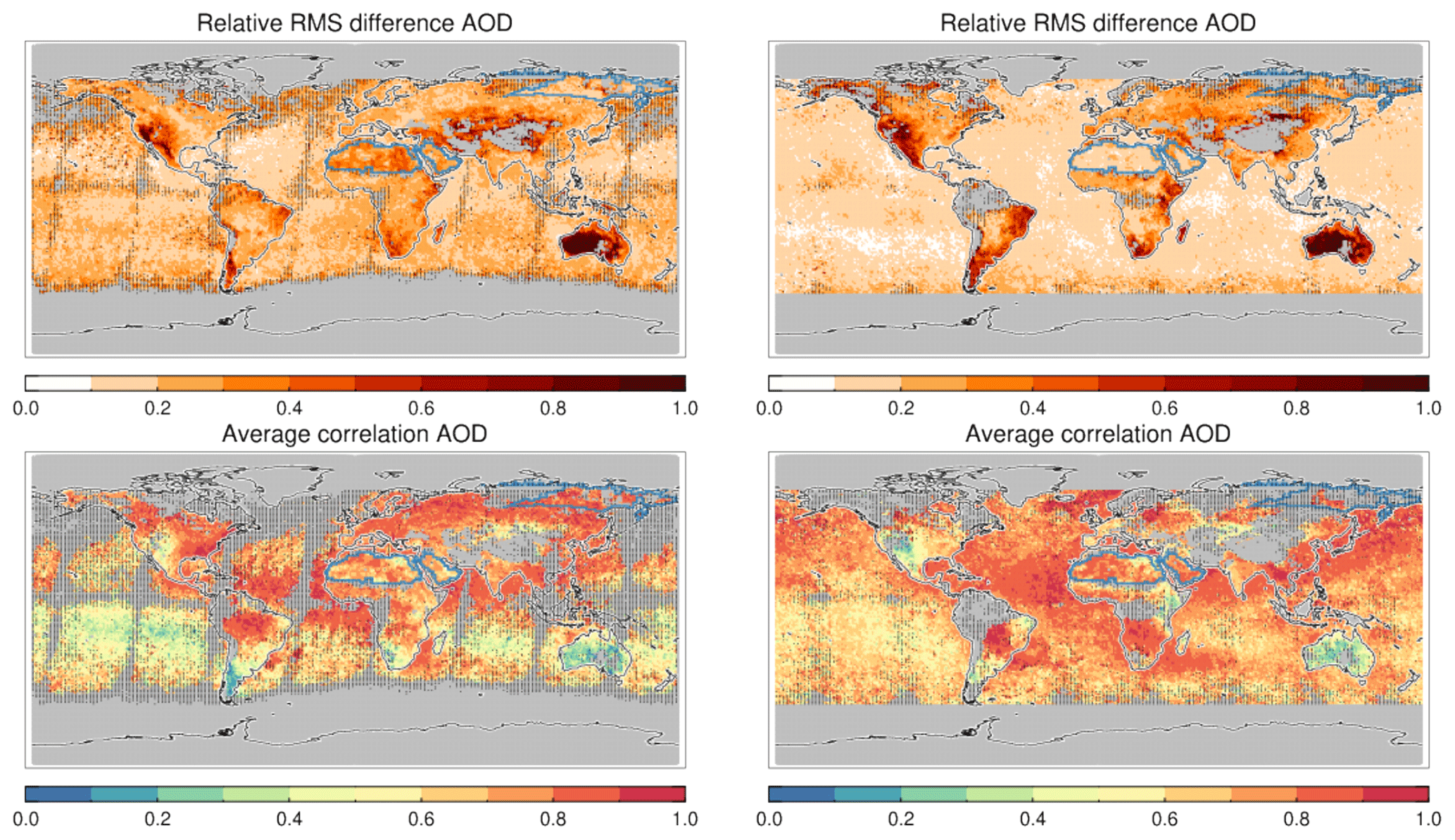
Figure 21 Global maps of relative diversity and average correlation of collocated satellite products. Diversity is the spread in AOD over the mean AOD. The average correlation is the average over all pair-wise correlations possible. Dotted areas indicate that the uncertainty due to statistical noise (standard deviation) is at least 0.1 (or fewer than 10 super-observations for each product were available). Over land, all seven products are used (blue contours identify areas of exception); over ocean at most four products are used (see text). Morning (left) and afternoon (right) products were collocated within 3 h.

Diversity is generally lowest over ocean, never reaching over 30 %, while over land, values of 100 % are possible. Over ocean, diversity is lowest for the afternoon products, presumably because only three products contribute (Aqua-DT, SeaWiFS and AVHRR) and two (SeaWiFS and AVHRR) use a similar algorithm (SOAR). The spatial distribution of diversity is fairly smooth over ocean, in contrast to land where one sees a lot of structure. This was also seen in the intercomparison of satellite products in Sect. 6. For an earlier study of satellite AOD diversity, see Chin et al. (2014), in which a different definition of diversity, a different (and smaller) set of satellite products and a different (sub-optimal) collocation procedure led to rather different magnitudes and spatial patterns of diversity. In contrast, the diversity presented in Sogacheva et al. (2019), while using a different definition and a different (sub-optimal) collocation procedure, agrees more with the one presented in Fig. 21 (there is substantial overlap in the satellite products used here and in Sogacheva et al., 2019; see Tables 1 and 2).

Also shown is the average correlation, i.e. the average of the correlation between all possible pairs of collocated products. Over the deep ocean (e.g. Southern Hemisphere Pacific Ocean) correlations are low. It seems that only in outflow regions (e.g. Amazonian outflow, southern African outflow, outflow from Sahara and African savannah, Asian outflow) will the products strongly agree in their temporal signal over ocean. This suggests that the correlation depends on the strength of the AOD signal (see also Sect. 5 and Fig. 5). Over land, the correlation shows more variation. Interestingly, the correlation is high when the diversity is low and vice versa: e.g. Australia shows high diversity in 3-year mean AOD and very low correlation between individual AOD data. This suggests that the same factor(s) that causes errors in 3-year averages also causes random errors in individual AOD.

The above results are pretty robust. For example, by excluding OMAERUV (arguably the product with the largest errors due to its large pixel sizes and extrapolation from UV wavelengths) from this analysis, the afternoon diversity over land looks even more like the morning diversity. Diversity maps for two other collocations (all AATSR products or all Aqua products) are shown in Fig. S7. The Aqua maps look similar to before, but diversity is more muted for the AATSR products (but notice the same spatial patterns).

Diversity is an ensemble property of seven collocated products and can be interpreted based on other ensemble properties: the mean AOD and the relative spread in spatial coverage; see Fig. 22. We interpret the mean AOD as an indication of the signal-to-noise ratio in the satellite retrievals and the spread in the spatial coverage as uncertainty in cloud masking. We see that the diversity goes down when the signal-to-noise ratio increases and goes up when the uncertainty in cloud masking increases. This is as one would expect. Notice that, for the majority of locations, the actual diversity varies only from ∼20 % to ∼50 %, e.g. no more than a factor 2.5.

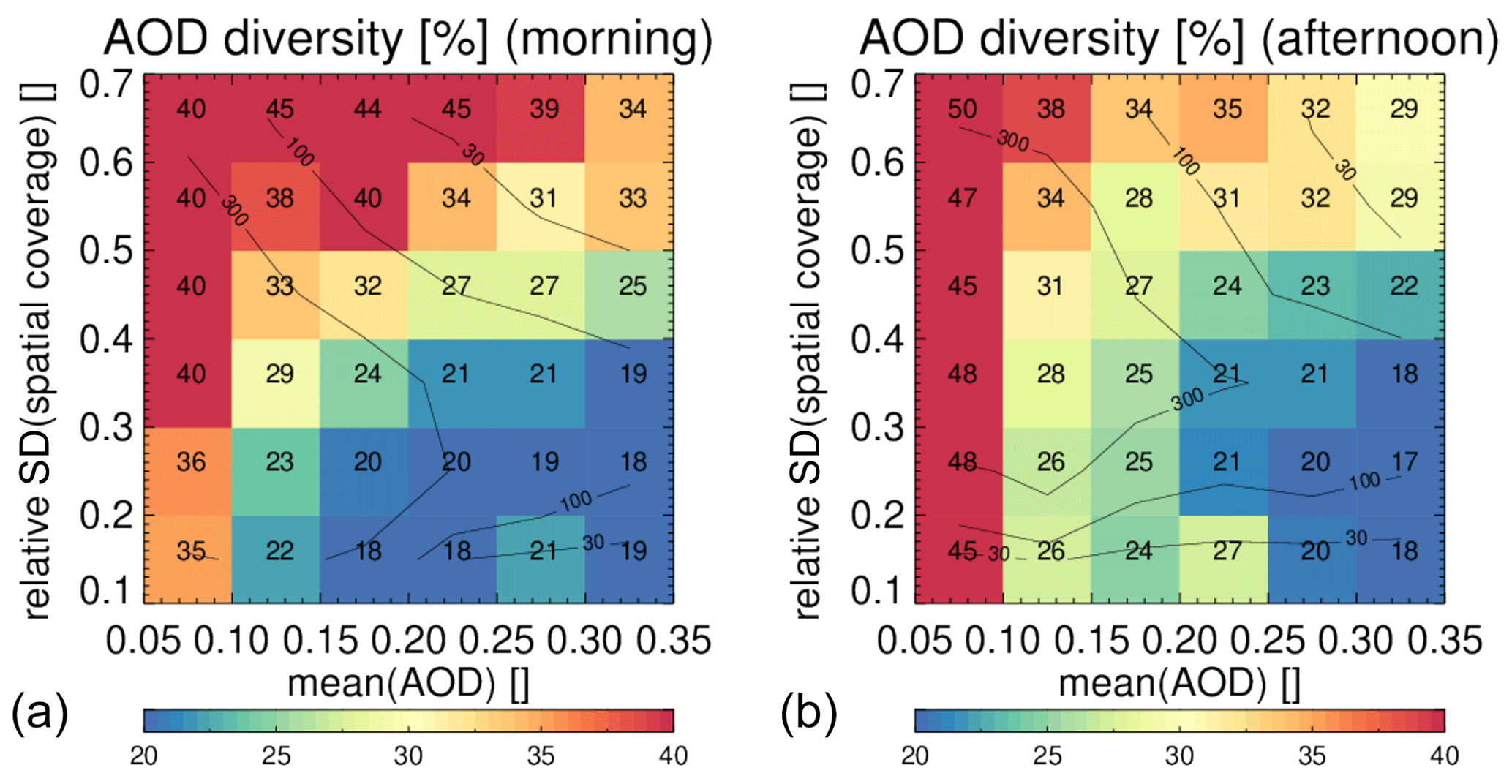
Figure 22 Diversity in AOD amongst morning and afternoon products as a function of mean AOD and the relative standard deviation in spatial coverage. The values in each bin show averaged diversity (similar to the colour). The contour lines show data density. Morning (a) and afternoon (b) products were collocated within 3 h. The statistics are dominated by observations over land. Over ocean, similar patterns are found but the range in diversity is much reduced.

Diversity turns out to be more than just the spread across multiple satellite products. The absolute diversity δ in the satellite AOD can actually be interpreted as the uncertainty ${\stackrel{\mathrm{‾}}{\mathit{\sigma }}}_{\mathrm{sat}}$ in multi-year averaged satellite AOD, at least in a statistical sense. Taking the 3-year averaged differences between a satellite and AERONET AOD (per site) from Sect 5 and dividing them by the diversity in the satellite ensemble (at that site), these normalized errors,

$$\begin{array}{}\text{(2)}& {\stackrel{\mathrm{‾}}{\mathit{ϵ}}}_{\mathrm{norm}}={\displaystyle \frac{{\stackrel{\mathrm{‾}}{\mathit{\tau }}}_{\mathrm{sat}}-{\stackrel{\mathrm{‾}}{\mathit{\tau }}}_{\mathrm{A}}}{\mathit{\delta }}},\end{array}$$

exhibit Gaussian distributions with standard deviations close to 1; see Fig. 23. We assume that in 3-year averages, both AERONET observation errors and representation errors are negligible. We conclude that $\mathit{\delta }\approx {\stackrel{\mathrm{‾}}{\mathit{\sigma }}}_{\mathrm{sat}}$, the latter being the uncertainty in satellite multi-year AOD. To put it differently, the multi-year AOD error can be statistically modelled as a random draw from a distribution with the absolute diversity as standard deviation. This works very well for Aqua-DT, DB, BAR, SeaWiFS and AATSR-SU products. It works less well for Aqua-MAIAC, which shows a global bias (identified before; see Sect. 5) but still has a normalized error with standard deviation close to 1. The Terra and AVHRR products show larger spread in the normalized error, while AATSR-ORAC and OMAERUV show significantly larger spread. It seems that the products that do better in the evaluation (Figs. 3 and 19) have errors that behave according to the diversity.

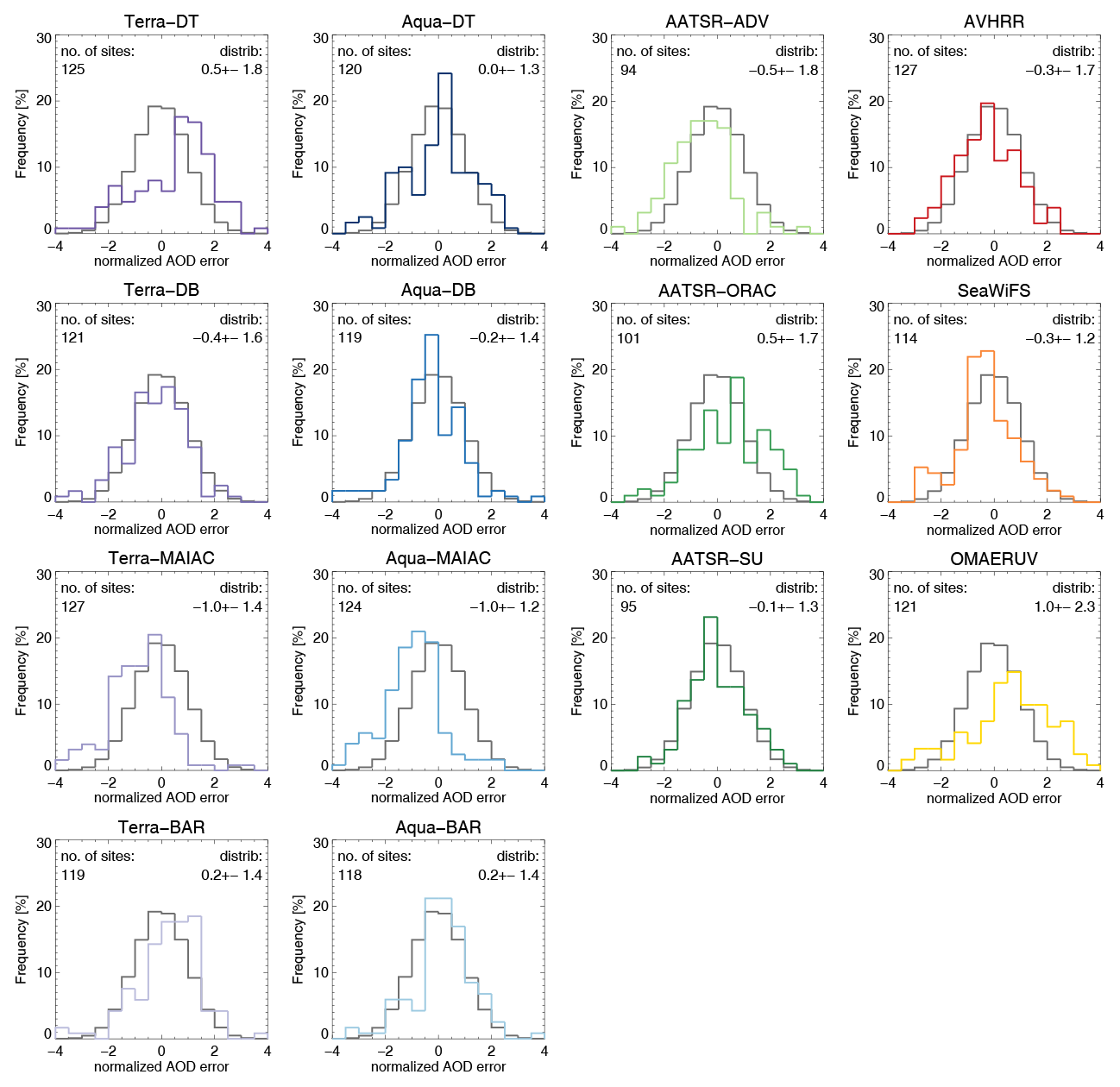
Figure 23 The 3-year averaged AOD error distributions, normalized to the diversity (spread in the ensemble; see Fig. 21). Errors are based on individual collocations of products with AERONET (within 1 h), unlike the diversity which is based on collocation of either all morning or afternoon satellite products together. Mean and standard deviation of the product's distribution are shown in the upper left corner. Only sites with at least 32 observations were used. For comparison, a normal distribution with mean zero and standard deviation of 1 is also shown (in black).

The conclusion that, in the current satellite ensemble, satellite AOD uncertainty may be modelled from satellite AOD diversity is probably the most important finding of this study and allows for several useful applications which will be discussed in Sect. 8. The diversity in AOD amongst satellite products has been published and is available as a download; see Schutgens (2020).

8 Summary

A detailed evaluation and intercomparison of 14 different satellite products of AOD is performed. Compared to previous studies of this kind (excl. Sogacheva et al., 2019), this one includes more (diverse) products and considers longer time periods, as well as of course more recent satellite retrieval products. Unlike previous studies it explicitly addresses the issue of uncertainty due to either statistical noise or sampling differences in datasets. While satellite products are assessed at both daily and multi-year timescales, the purpose of this study is to understand satellite AOD uncertainty in the context of model evaluation. In practice this means $\mathrm{1}{}^{\circ }\times \mathrm{1}{}^{\circ }$ aggregates (or super-observations) of the original retrievals are evaluated for their multi-year bias.

The 14 satellite products include retrievals from MODIS (Terra/Aqua), AATSR (ENVISAT), AVHRR (noaa18), SeaWiFS (SeaStar) and OMI (Aura). Two other products, based on POLDER (PARASOL), are part of the database but were not included in the current paper. They will be reported on in a follow-up paper. Two other products, MISR (Multi-angle Imaging SpectroRadiometer) and VIIRS (Visible Infrared Imaging Radiometer Suite), are also not part of the current AeroCom–AeroSat study (MISR was in the middle of an update cycle, and VIIRS was only launched in 2011). Four different MODIS and three different AATSR retrieval algorithms were used. The over-land products from AVHRR, SeaWiFS and one MODIS product use variations of the same algorithm (Deep Blue).

The evaluation is made with AERONET and MAN observations. Only AERONET sites with good spatial representativity and maintenance records were selected, based on a previously published list by Kinne et al. (2013). The suitability of these sites was further assessed by “evaluating” them against the ensemble of satellite products, which led to the identification of four sites that show substantially different AOD than any satellite dataset. Whether these sites are unsuitable for satellite evaluation or all products retrieve AOD poorly over those sites is an open question, but we removed them from our selection of AERONET sites. Lastly we used the satellite observations themselves to confirm that representation errors, while not negligible, are a minor contribution to the difference between satellite ($\mathrm{1}{}^{\circ }\times \mathrm{1}{}^{\circ }$ aggregates) and AERONET AOD.

For evaluation and intercomparison purposes, different data products were collocated within a few hours. Sensitivity studies show this provides a good trade-off between accuracy and data amount. We make extensive use of bootstrapping to assess the uncertainty ranges in our error metrics due to statistical noise. We try to address uncertainty due to the spatial sparsity of AERONET and MAN data, preventing a true global analysis, through satellite product intercomparisons.

All satellite daily AOD data show good to very good correlations with AERONET ($\mathrm{0.73}\le r\le \mathrm{0.89}$), while global biases vary between −0.04 and 0.04. In 3-year averaged AOD, site-specific biases can be as high as 50 % (either positive or negative), although a more typical value is 15 % for the top-performing products and 25 % for the products that perform less well (in absolute values: 0.025 to 0.040). These site-specific biases show regional patterns of varying sign that together cause a balancing of errors in the traditional global bias estimate of satellite AOD, which may not be a very useful metric for satellite AOD performance. In addition to these biases, satellite products also exhibit random errors that appear to be at least 1.6 to 3 times larger than the site-specific biases. Evaluation of satellite products on a daily timescale (dominated by random errors rather than biases) therefore gives only limited information on the usefulness of a product for global multi-year model evaluation. While evaluation results for AERONET are usually robust, considerable uncertainty remains in the evaluation by MAN data due to the low data count (3 years of data).

The satellite intercomparison confirms the previous evaluation but extends its spatial scope. Daily satellite data usually correlate very well with other satellite products, and 3-year averages show regional patterns in product differences. These patterns can often, but not always, be linked to major orography. In any case, the patterns show large spatial scales which should aid in the identification of their causes. Over ocean, product differences are both smaller and spatially smoother, with a latitudinal dependence. The best agreement in AOD is found when using the same algorithm for the same sensor on two different platforms (Terra/Aqua). Large differences in AOD can be found for products using different algorithms but on the same platform and for the same sensor (MODIS on either Aqua or Terra, or AATSR on ENVISAT). Already variations in the same algorithm can lead to substantially different AOD data (Deep Blue for MODIS, AVHRR and SeaWiFS).

Although the aggregated AOD correlates quite well among satellite products, we were able to show that the area covered in each $\mathrm{1}{}^{\circ }\times \mathrm{1}{}^{\circ }$ grid box (called spatial coverage) correlates significantly less well among the products. We present evidence that this spatial coverage is determined mostly by (observed) cloud fraction and suggest there may be substantial differences in the quality of cloud screening by the different products. The evidence consists of the following observations: (1) biases vs. AERONET decrease with increasing coverage; (2) correlations with AERONET increase with increasing coverage; and (3) satellite differences decrease with increasing coverage. The simplest explanation (Ockham's razor) would be that coverage is the complement of cloud fraction, and as coverage goes down, cloud fraction (and cloud contamination) goes up. Product differences at low spatial coverage (high cloud fraction) are about twice as large than at high spatial coverage (low cloud fraction).

Intercomparing the product evaluation (with AERONET) of satellite products is challenging. A true apples-to-apples comparison requires collocating all datasets (including AERONET), but this greatly reduces the number of data available for analysis. As a consequence, it is likely that those data sample only part of the underlying true error distribution. We showed that an apples-to-apples comparison leads to different results (compared to an individual collocation with AERONET) for some datasets but no great changes for others. As we were able to show, this is unlikely the result of statistical noise; we seem forced to conclude that a true comparison of product skill is only possible for a limited set of circumstances.

Collocating either the morning or afternoon products together allows us to create maps of 3-year averaged AOD diversity amongst the products. Although there are differences, the diversity for morning and afternoon products shows similar patterns and magnitudes. Diversity shows a lot of spatial variation, from 10 % over parts of the ocean to 100 % over parts of central Asia and Australia. Also, in a broad statistical sense, diversity can be shown to relate to the retrieval signal-to-noise ratio and uncertainty in cloud masking within the $\mathrm{1}{}^{\circ }\times \mathrm{1}{}^{\circ }$ grid boxes of super-observations. The most interesting find, however, is that diversity can be used to predict uncertainty in 3-year averaged AOD of individual satellite products (at least for the better performing products).

The possible applications of diversity and its interpretation as uncertainty are multiple. First, diversity shows (by definition) where satellite products differ most and thereby offers clues on how to improve them. Second, for the same reason, diversity may be used as guidance in choosing future locations for AERONET sites. Observations at locations with large diversity offer more information on individual satellite performance than those from locations with small diversity. Third, diversity as uncertainty provides a spatial context to the product evaluation with sparse AERONET sites. Fourth, and related to third, diversity as uncertainty offers a very simple way to evaluate and intercompare new satellite products to the 14 products considered in this study. To perform better than these products, their normalized multi-year difference from AERONET (Eq. 2) should exhibit a standard deviation smaller than 1 (see Fig. 23). Fifth, again related to third, diversity as uncertainty offers modellers a simple estimate of the expected multi-year average uncertainty in satellite AOD. The diversity in AOD amongst satellite products has been published and is available as a download; see Schutgens (2020).

Appendix A: Generic aggregation and collocation

The aggregation of satellite L2 products into super-observations in this paper, and the subsequent collocation of different datasets for intercomparison and evaluation, used the following scheme.

Assume an L2 dataset with times and geolocations and observations of AOD. Each observation has a known spatio-temporal footprint; e.g. in the case of satellite L2 retrievals, that would be the L2 retrieved pixel size and the short amount of time (less than a second) needed for the original measurement.

Satellite L2 data are aggregated into super-observations as follows. A regular spatio-temporal grid is defined as in Fig. A1. The spatio-temporal size of the grid boxes (here 30 min × $\mathrm{1}{}^{\circ }\times \mathrm{1}{}^{\circ }$) exceeds that of the footprint of the L2 data that will be aggregated. All observations are assigned to a spatio-temporal grid box according to their times and geolocations. Once all observations have been assigned, observations are averaged by grid box. It is possible to require a minimum number of observations to calculate an average. Finally, all grid boxes that contain observations are used to construct a list of super-observations as in Fig. A2. Only times and geolocations with aggregated observations are retained.

Station data are similarly aggregated over 30 min × $\mathrm{1}{}^{\circ }\times \mathrm{1}{}^{\circ }$. Point observations will suffer from spatial representativeness issues (Sayer et al., 2010; Virtanen et al., 2018; Schutgens et al., 2016a), but the representativity of AERONET sites for $\mathrm{1}{}^{\circ }\times \mathrm{1}{}^{\circ }$ grid boxes is fairly well understood (Schutgens, 2019); see also Sect. 4. These aggregated L3 AERONET and MAN data will also be called super-observations.

Different datasets of super-observations can be collocated in a very similar way. Again a regular spatio-temporal grid is defined as in Fig. A1 but now with grid boxes of larger temporal extent (typically 3 h × $\mathrm{1}{}^{\circ }\times \mathrm{1}{}^{\circ }$). Because this temporal extent is short compared to satellite revisit times, either a single satellite super-observation or none is assigned to each grid box. A single AERONET site however may contribute up to six super-observations per grid box (in which case they are averaged). After two or more datasets are thus aggregated individually, only grid boxes that contain data for both datasets will be used to construct two lists of aggregated data as in Fig. A2. Those two lists will have identical size and ordering of times and geolocations and are called collocated datasets. By choosing a larger temporal extent of the grid box, the collocation criterion can be relaxed.

As the super-observations are on a regular spatio-temporal grid and collocation requires further aggregation to another regular, but coarser, grid, the whole procedure is very fast. It is possible to collocate all seven products from afternoon platforms over 3 years using an IDL (Interactive Data Language) code and a single processing core in just 30 min. This greatly facilitates sensitivity studies.

Starting from super-observations, a 3-year average can easily be constructed by once more performing an aggregation operation but now with a grid box of 3 years × $\mathrm{1}{}^{\circ }\times \mathrm{1}{}^{\circ }$. If two collocated datasets are aggregated in this fashion, their 3-year average can be compared with minimal representation errors. This allows us to construct global maps of, for example, the multi-year AOD difference between two sets of super-observations.

A software tool (the Community Intercomparison Suite) is available for these operations at http://www.cistools.net (last access: 20 December 2019) and is described in great detail in Watson-Parris et al. (2016).

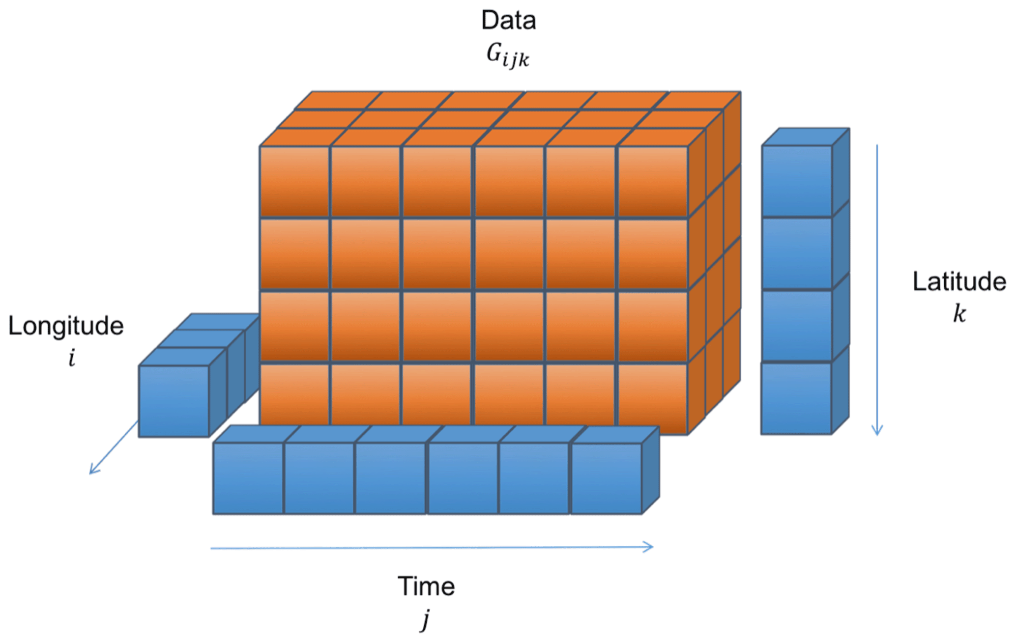
Figure A1 A regular spatio-temporal grid in time, longitude and latitude. Such a grid is used for the aggregation operation that is at the heart of the collocation procedure used in this paper. Grid boxes may either contain data or be empty. Reproduced from Watson-Parris et al. (2016).

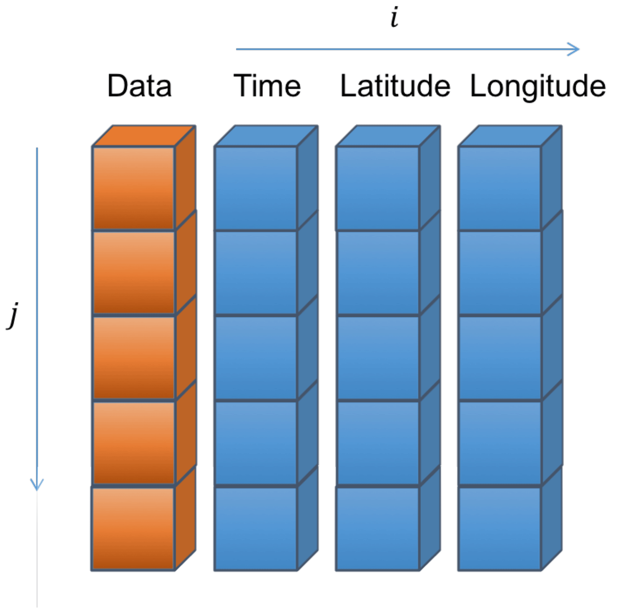
Figure A2 A list of data. Such a list is the primary data format used for both observations and model data in this paper. Reproduced from Watson-Parris et al. (2016).