The regional European atmospheric transport inversion comparison, EUROCOM: first results on European-wide terrestrial carbon fluxes for the period 2006–2015

Atmospheric inversions have been used for the past two decades to derive large-scale constraints on the sources and sinks of CO₂ into the atmosphere. The development of dense in situ surface observation networks, such as ICOS in Europe, enables in theory inversions at a resolution close to the country scale in Europe. This has led to the development of many regional inversion systems capable of assimilating these high-resolution data, in Europe and elsewhere. The EUROCOM (European atmospheric transport inversion comparison) project is a collaboration between seven European research institutes, which aims at producing a collective assessment of the net carbon flux between the terrestrial ecosystems and the atmosphere in Europe for the period 2006–2015. It aims in particular at investigating the capacity of the inversions to deliver consistent flux estimates from the country scale up to the continental scale.

The project participants were provided with a common database of in situ-observed CO₂ concentrations (including the observation sites that are now part of the ICOS network) and were tasked with providing their best estimate of the net terrestrial carbon flux for that period, and for a large domain covering the entire European Union. The inversion systems differ by the transport model, the inversion approach, and the choice of observation and prior constraints, enabling us to widely explore the space of uncertainties.

This paper describes the intercomparison protocol and the participating systems, and it presents the first results from a reference set of inversions, at the continental scale and in four large regions. At the continental scale, the regional inversions support the assumption that European ecosystems are a relatively small sink ($-\mathrm{0.21}\pm \mathrm{0.2}$ Pg C yr⁻¹). We find that the convergence of the regional inversions at this scale is not better than that obtained in state-of-the-art global inversions. However, more robust results are obtained for sub-regions within Europe, and in these areas with dense observational coverage, the objective of delivering robust country-scale flux estimates appears achievable in the near future.

1 Introduction

The carbon budget of Europe has been explored in several large-scale synthesis studies, such as the CarboEurope-Integrated Project (Schulze et al., 2009) and the REgional Carbon Cycle Assessment and Processes project (RECCAP; Luyssaert et al., 2012), to name a few. Although these have helped refine the knowledge of the European carbon cycle, large uncertainties remain regarding the quantification of the flux between terrestrial ecosystems and the atmosphere, usually quantified as the net ecosystem exchange (NEE), i.e. the sum of emissions (total ecosystem respiration (TER), i.e. autotrophic and heterotrophic respiration) and uptake (gross primary production (GPP), i.e. photosynthesis) of carbon by ecosystems to and from the atmosphere, or alternatively NBP (net biome production), which includes the impact of ecosystem disturbances (fires, land use change, etc.). For instance, Luyssaert et al. (2012) report average estimates of European land carbon sink in a −200 to −360 Tg C yr⁻¹ range for the years 2001–2005, depending on the estimation method, and each of these estimates is provided with large uncertainties (with 1σ relative uncertainties of 50 % to 100 %). Confronting the ensemble of results from different syntheses, Reuter et al. (2017) report annual land–atmosphere flux ranging from $-\mathrm{400}\pm \mathrm{420}$ up to $-\mathrm{1030}\pm \mathrm{470}$ Tg C yr⁻¹ in the 2000s. Beyond the annual long-term budget, the year-to-year annual flux variations are also poorly known (Bastos et al., 2016). In practice, the lack of a robust and precise quantification of the natural CO₂ fluxes in Europe limits our ability to understand the links between the NEE flux and external forcings such as, for example meteorological variability (including the impact of extreme events like droughts and cold spells) and trends (Ciais et al., 2005; Maignan et al., 2008) or land use change (Naudts et al., 2016), and to forecast the evolution of the land sink in Europe, in the context of global climate change.

Despite the large uncertainties, there is a growing demand from the policy makers and the society in general for more accurate and relevant numbers, such as estimates of the national budgets of CO₂ fluxes, these demands being reinforced by the Paris Agreement. For instance, the European Commission (under the VERIFY and CHE H2020 projects) is supporting the development of observation-based monitoring systems for estimating CO₂ fluxes at national to sub-national scales, with a clear interest in both land ecosystem fluxes and anthropogenic emissions.

Atmospheric transport inversions rely on transport models and statistical methodologies to derive the most likely estimates of CO₂ fluxes given large datasets of observed atmospheric CO₂ concentrations and prior information provided in general by ecosystem models. Global inversion systems, using coarse-resolution global transport models (typically >2^∘) have so far been the dominant tool for producing top-down estimates of NEE fluxes. The coordination of the inverse modelling community through intercomparison exercises with ≈10 global inverse modelling systems, such as that conducted in the frame of the TRANSCOM and RECCAP projects (Law et al., 1996; Gurney et al., 2002; Patra et al., 2008; Peylin et al., 2013) have been valuable for understanding the strengths and weaknesses of global inversions and to characterize the real uncertainty of the different estimates. However, despite this long-term effort, global inversions remain limited by the coarse resolution of the transport models they rely on, as these do not allow a proper representation of observation sites in regions with complex orography or nearby large anthropogenic CO₂ emissions and do not reproduce the high-resolution spatial variability of the CO₂ concentrations that is captured by dense networks.

Regional-scale inversions started to emerge about a decade ago. They rely on mesoscale transport models (at 1^∘ down to 10 km resolution), capable of better representing the spatial and temporal variability of concentrations observed by dense networks of CO₂ observations, such as that of the Integrated Carbon Observation System (ICOS) in Europe. In particular the models should be able to account for CO₂ fluxes at a scale that does not smooth too much the hot spots of fossil fuel CO₂ emissions in cities and industrial areas. They demonstrated some potential to solve for continental to subcontinental budgets at the monthly scale (e.g. Peters et al., 2007; Rödenbeck et al., 2009; Schuh et al., 2010; Gourdji et al., 2012; Broquet et al., 2013; Meesters et al., 2012). However, until recently, there has only been limited efforts to routinely perform regional inversion estimates in Europe (partly owing to the difficult access to long-term time series of quality-controlled CO₂ data). Most published synthesis studies have therefore relied on European NEE estimates from global-scale inversions, based on global networks of mostly background sites.

The ICOS atmospheric network (https://icos-atc.lsce.ipsl.fr, last access: 6 August 2020) is now operational and its number of stations should regularly increase from the current 19 labelled stations towards at least 37 sites, currently run by 12 and hopefully in the future more European member states. Precursor networks such as those set up in the framework of the CarboEurope and GHG-Europe projects (Ramonet et al., 2010) and the ICOS preparatory phase provide a robust basis for regional inversions during the pre-ICOS decade. The ICOS Carbon Portal (https://www.icos-cp.eu, last access: 6 August 2020) has been set up to support the exchange of observational data and elaborated products related to the carbon cycle, such as CO₂ fossil fuel flux maps. In addition to in situ data, the development of satellite observations of CO₂ following the launch of GOSAT (Kuze et al., 2009) in 2009 and OCO-2 in 2014 (Crisp et al., 2004) should further densify the observation coverage, in particular with the foreseen European constellation of CO₂ high-resolution imagers of the Copernicus Anthropogenic CO₂ Monitoring mission (CO2M; Pinty et al., 2017), starting from 2025. The use of mesoscale transport models will then become necessary to fully exploit the potential of these large datasets with observations at high spatial and temporal resolution.

In this context, the EUROCOM (EUROpean atmospheric transport inversion COMparison) project aims to coordinate a European effort to improve the knowledge on the NEE based on an ensemble of long-term European-scale inversions (i.e. covering geographical Europe). The project involved the participation of seven research groups, which have produced an ensemble of more than (to date) 12 inversions (including sensitivity experiments), estimating the European NEE for the period 2006–2015 following a protocol described further in this document. The EUROCOM project is therefore one of the first regional inversion intercomparisons, and the first one at such a scale dedicated to the European NEE.

The first task of the project, to which this paper is dedicated, is to assess the capacity of regional inversions to robustly estimate European NEE. We focus on key diagnostics which are typically looked at in synthesis studies, such as the annual and monthly budgets of NEE and the inter-annual variability, for all of Europe and for large regions. We use the results from an ensemble of six inversions (one for each participating system), covering a large spectrum of inversion characteristics (prior constraints, inversion technique, transport models, etc.): PYVAR-CHIMERE (Broquet et al., 2011; Fortems-Cheiney et al., 2019, developed at LSCE, France); LUMIA (Lund University Modular Inversion Algorithm) (Monteil and Scholze, 2019), developed at Lund University (Sweden) as part of the EUROCOM project; CarboScope-Regional (Kountouris et al., 2018a, b, developed at MPI-Jena, Germany); FLEXINVERT (Thompson and Stohl, 2014, from NILU, Norway); NAME-HB (White et al., 2019b, from the University of Bristol, United Kingdom) and CarbonTracker Europe (Peters et al., 2010; van der Laan-Luijkx et al., 2017), from the University of Wageningen, the Netherlands.

The EUROCOM project extends beyond the scope of this paper. Forthcoming studies using a larger ensemble of inversions (including additional sensitivity experiments) will focus on quantifying and reducing specific aspects of the uncertainty, supporting the improvement of both the regional inversion techniques and the design of the European observation network.

The paper is organized in five sections. Section 2 briefly summarizes the theoretical background behind atmospheric transport inversions. Section 3 details the inversion protocol, the participating inverse modelling systems and the input products (fluxes and observations) shared within EUROCOM for conducting the inversions. Results are presented in Sect. 4 and then discussed in Sect. 5. Finally, Sect. 6 summarizes the paper and provides some remarks on the future of the EUROCOM collaboration, and on regional inverse modelling in general.

2 Inverse modelling methodology and terminology

The theoretical framework of the atmospheric inverse transport modelling has been extensively detailed in past publications (e.g. Enting, 2002; Rayner et al., 2019). Here we only give a brief overview of the basic principles, to facilitate the comprehension of the paper for readers unfamiliar with the approach and to remind of some of the components discussed in detail in Sect. 3.

Bayesian atmospheric inversions rely on the fact that observed spatio-temporal gradients of CO₂ in the atmosphere reflect the distribution of carbon exchanges between the atmosphere and other carbon reservoirs. The link between the net CO₂ exchange at the surface and the CO₂ concentrations in the atmosphere is established by a forward atmospheric transport model. A first set of modelled CO₂ concentrations (y^m=H(x)) is computed at the time and location of real observations (y^o), based on a prior assumption of what the CO₂ fluxes are (x_b). The mismatch between the modelled and observed concentrations ($\mathit{\delta }y=H\left(\mathit{x}\right)-{\mathit{y}}^{\mathrm{o}}$) is used to derive a correction δx to the prior flux estimate x_b. The posterior flux estimate ($\mathit{x}={\mathit{x}}_b+\mathit{\delta }x$) then represents the best statistical compromise between fitting the observations and limiting the departures to the prior, accounting for the statistical distribution of uncertainties in both observations and prior fluxes.

The vector x is called the control vector. It contains all the parameters that the inversion can adjust. In our case it contains at least the terrestrial ecosystem component of the CO₂ fluxes. It can also contain other adjusted parameters such as bias or boundary concentration terms. The operator H, which establishes the deterministic relationship between a given control vector x and the corresponding modelled concentrations y^m is called the observation operator. It encompasses the transport model, but also the impact on the modelled concentrations of any input of the transport model that is not further adjusted in the inversions (prescribed anthropogenic emissions, boundary conditions, etc.).

Following the Bayesian approach and using a classical Gaussian error hypothesis the problem is reduced to finding the posterior control vector x_a that minimizes the cost function J(x), defined as follows:

$$\begin{array}{}\text{(1)}& J\left(\mathit{x}\right)=\underset{J_b}{\underbrace{{\displaystyle \frac{\mathrm{1}}{\mathrm{2}}}\mathit{\delta }{\mathit{x}}^T{\mathbf{B}}^{-\mathrm{1}}\mathit{\delta }\mathit{x}}}+\underset{J_{\mathrm{obs}}}{\underbrace{{\displaystyle \frac{\mathrm{1}}{\mathrm{2}}}\mathit{\delta }{\mathit{y}}^T{\mathbf{R}}^{-\mathrm{1}}\mathit{\delta }\mathit{y}}}.\end{array}$$

The prior error covariance matrix B contains a representation of the uncertainties on the prior control vector x_b and the error covariance matrix R contains the observational error, which combines the measurement uncertainties (uncertainty of the observations y) and the uncertainties associated with the observation operator H: the representation error (due to the comparison of point concentration measurements with gridded model concentration) and the model error (uncertainty in non-optimized model parameters, such as the boundary and initial conditions, the non-optimized fluxes, and uncertainty in the model physics). Departing from the prior control vector x_b increases J_b, and improving the fit to the observations reduces J_obs. B and R modulate the relative weight of each departure to the prior and to the observations in J.

The exact specifications of B and R affect to a certain extent the outcome of an inversion. For practical reasons, the error covariance matrix for the observations R is usually defined as a diagonal matrix with the measurement and model uncertainty (σ) for each observation site specified on the diagonal. Potential error correlations between observations are typically dealt with by limiting the density of observations or inflating their individual uncertainties. The diagonal elements of the prior error covariance matrix B contains the uncertainties of the prior control parameters (typically here the NEE at the grid scale). The off-diagonal elements, corresponding to the covariances between uncertainties in different control parameters, are difficult to specify because the uncertainties in the NEE estimates have hardly been characterized and quantified (Kountouris et al., 2015). They are, however, a critical component of the inversion as they determine how independently from each other the different components of the control vector can be adjusted. The inversions in this study follow different implementations of this general methodology, listed in Sect. 3.3.2.

The optimal control vector x_a can be solved for using different solution methods. Here we only briefly recall the methods employed by the systems in this study (variational and sequential ensemble approaches, and Markov Chain–Monte Carlo); more information on these methods is given in Rayner et al. (2019) and references therein.

The variational method minimizes J(x) based on iterative gradient descent methods. Efficient implementations of this method rely either on the availability of the adjoint of the transport model or pre-computed transport Jacobian matrices representing the sensitivity of the observation vector to the control vector. The Monte Carlo approach directly samples the cost function, and in the case of the Markov chain–Monte Carlo (MCMC) approach, the samples form a Markov chain; i.e. each sample is not obtained independently, but rather a perturbation of the last previously accepted sample. This allows non-Gaussian PDFs to be used in the inversion and allows the specification of uncertainties to be explored in so-called “hierarchical” Bayesian frameworks (Ganesan et al., 2014; Lunt et al., 2016). Finally, the ensemble Kalman filtering (EnKF) directly derives x^a following its analytical formulation based on the reduction of the dimensions of the problem through the split of the inversion into sequential windows, and based on the computation of the matrices involved in the EnKF formulation through an ensemble Monte Carlo approach.

3 Protocol and participating models

Given the overall objective of the study (to assess the robustness of inversion-derived European flux estimates), we deliberately opted for a relatively loose protocol: the participants were requested to use a common set of anthropogenic CO₂ emissions (fossil fuel combustion, cement production and large-scale fires) and to use only atmospheric observations from a common dataset, prepared specifically for the EUROCOM project (Sect. 3.1). They were requested to provide a monthly gridded estimate of the net land–atmosphere CO₂ exchange (net ecosystem exchange, NEE) over the period 2006 to 2015, covering at least the area 15^∘ W–35^∘ E by 33–73^∘ N, at a 0.5^∘ by 0.5^∘ spatial resolution (independently of the actual resolution of the inversions).

A set of fluxes (prior NEE, anthropogenic and ocean fluxes) was made available to the modellers through a data repository hosted at the ICOS Carbon Portal, along with the common observation database, but except for the imposed anthropogenic emissions, the participants were essentially free to choose the characteristics of their inversions. In particular they could perform further selections on the observations database (selection of observation sites and selection of observations to use at each site) and choose their prior NEE and ocean flux estimates. The treatment of boundary conditions and the precise specification of uncertainties (prior and observation uncertainties) were also left to the modellers.

The inversions in our ensemble are constructed with the aim to maximize the diversity of the systems, and hence to obtain a better estimate of the overall uncertainty of inversion results. A stricter protocol, for example fixing the prior fluxes and the prior uncertainties, would facilitate the interpretation of results but would artificially decrease their spread. Furthermore, some parameters should not be prescribed. For instance, the observations are selected based on the capacity of the underlying transport model to reproduce them, and the type of boundary condition is also dependent on the transport models, which differ across the systems. It is, however, clear that further steps will be needed, with a stricter protocol, to fully understand the specific causes of the discrepancies that were obtained.

3.1 Common atmospheric observation database

A comprehensive dataset of atmospheric CO₂ concentration observations in Europe was compiled as input for the inversion systems, on the basis of the GLOBALVIEWplus v3.2 Observation Package (ObsPack), a product compiled and coordinated at NOAA's Earth System Research Lab together with the ICOS Carbon Portal (Cooperative Global Atmospheric Data Integration Project, 2017). The dataset was further extended by including measurements that had been collected in several national and EU-funded projects, like CarboEurope-IP and GHG-Europe, and during the preparatory phase of the Integrated Carbon Observation System (ICOS) Research Infrastructure. Finally, for two stations, the data were obtained from the World Data Center for Greenhouse Gases (https://gaw.kishou.go.jp/, last access: 6 August 2020).

Table 1 Observation sites used in the inversions. Datasets with in situ continuous (C) as well as flask (F) measurements were taken from GLOBALVIEWplus ObsPack, WDCGG, and the EU-funded projects CarboEurope-IP, GHG-Europe and ICOS preparatory phase (all indicated as pre-ICOS).

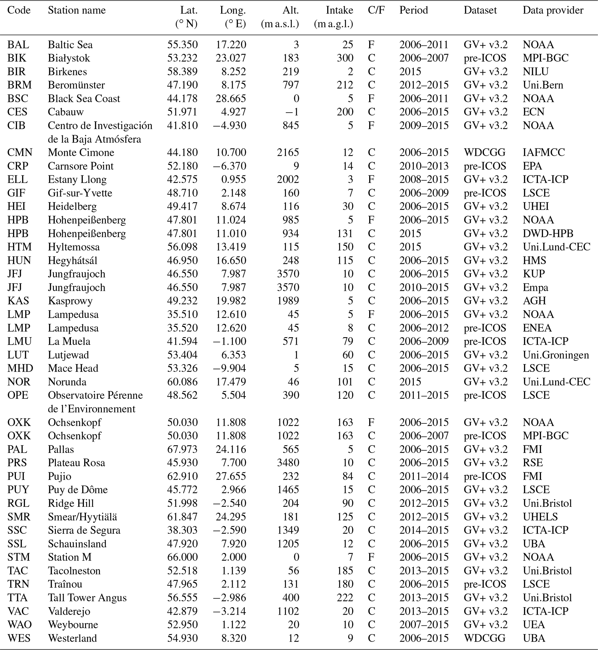
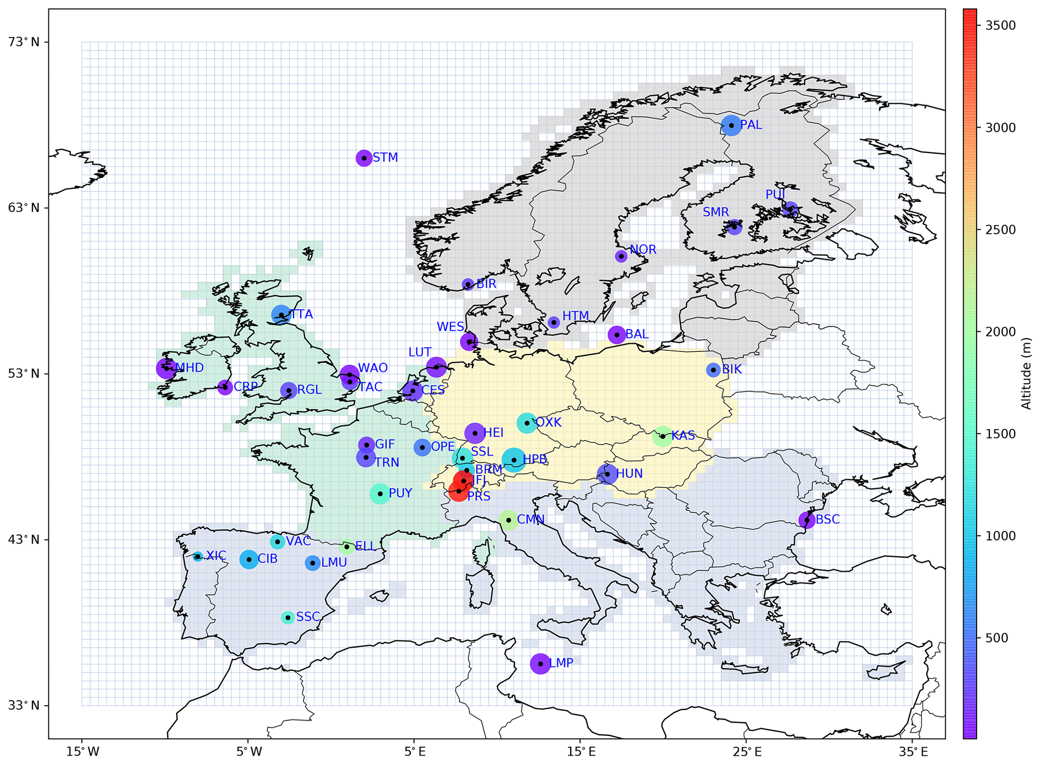
Figure 1 EUROCOM domain (pale blue grid with the 0.5^∘ resolution) and location of the observation sites. The size of the dots is proportional to the number of months with at least one observation available (in the common observation database, not all observations are used in the inversions), and the colour map shows the altitude of the sites (height above ground + sampling height). The four regions used in the analysis are also represented: western Europe (green), southern Europe (blue), central Europe (yellow) and northern Europe (grey).

Compared to the original GLOBALVIEWplus product, we added time series from nine measurement stations and partly complemented time series at two stations. The datasets were harmonized with respect to format and sampling interval and provided in the ObsPack format (Masarie et al., 2014). The original datasets and data providers of the time series are reported in Table 1, and the locations of the observation sites are also shown in Fig. 1.

The majority of sites (35 out of 39) sample concentrations continuously (i.e. hourly or more frequently); 18 sites are tall towers (intake height >50 m), some with observations available at different levels, in which case only the upper level was used (as it is more difficult for the transport models to represent concentration gradients close to the ground).

The modellers were free to refine the observation selection according to the ability of their inversion systems to simulate specific stations, and in particular to use their preferred approach to select data within a day (i.e. use of all the observations within a time frame or use of an average of the observations, etc.). The precise observation selection approaches are discussed further in Sect. 3.3.3, and a full comparison of the observation assimilated by each system is provided in Figs. S1 and S2 in the Supplement.

3.2 Prior and prescribed CO₂ fluxes

All groups split the total surface–atmosphere CO₂ flux in three or four categories: biosphere (NEE, optimized), ocean (sea–atmosphere CO₂ exchanges, prescribed or optimized), anthropogenic (prescribed) and biomass burning (prescribed, used by LUMIA and FLEXINVERT+).

Note that we use the term NEE (sum of photosynthesis and ecosystem respiration) for the posterior fluxes over land throughout the paper, because this is what the prior flux estimates from the terrestrial ecosystem models represent. However, strictly speaking, the inversions optimize the flux that is not explained by the prescribed anthropogenic (and sometimes ocean) fluxes. This includes the effect of ecosystem disturbances (land use, land management, biotic effects) but also projection of errors in the prescribed fluxes.

3.2.1 Terrestrial-ecosystem fluxes

Atmospheric inversions usually rely on NEE simulations from terrestrial ecosystem models to provide the prior value of the NEE component of the control vector (as defined above in Sect. 2). Within EUROCOM four different simulations of gross (GPP and ecosystem respiration) and net (NEE) terrestrial biosphere fluxes were included: three from process-based models (ORCHIDEE, LPJ-GUESS and SiBCASA), and one from a diagnostic model (VPRM). Two of the four models (ORCHIDEE and LPJ-GUESS) are providing input for the Global Carbon Project annual global CO₂ assessment (Le Quéré et al., 2018).

• ORCHIDEE (used by PYVAR-CHIMERE, FLEXINVERT+ and NAME-HB): ORCHIDEE (Krinner et al., 2005) computes carbon, water and energy fluxes between the land surface and the atmosphere and within the soil–plant continuum. The model computes the gross primary productivity with the assimilation of carbon based on Farquhar et al. (1980) for C₃ plants. Land cover changes (including deforestation, regrowth and cropland dynamic) were prescribed using annual land cover maps derived from the harmonized land use dataset (Hurtt et al., 2011) combined with the ESA-CCI land cover products. The ORCHIDEE simulation used here has been produced at a global, 0.5^∘ resolution with 3-hourly output.

• LPJ-GUESS (used by LUMIA): LPJ-GUESS (Smith et al., 2014) combines process-based descriptions of terrestrial ecosystem structure (vegetation composition, biomass and height) and function (energy absorption, carbon and nitrogen cycling). Vegetation is dynamically simulated as a series of replicate patches, in which individuals of each simulated plant functional type (or species) compete for the available resources of light and water, as prescribed by the climate data. LPJ-GUESS includes an interactive nitrogen cycle. The simulation used here is forced using the WFDEI meteorological dataset (Weedon et al., 2014) and produces a 3-hourly output of gross and net carbon fluxes at a 0.5^∘ horizontal resolution.

• SiBCASA (used by CTE): SiBCASA (Schaefer et al., 2008) combines the parameterization of the Simple Biosphere model (SiB) with the biogeochemistry of the Carnegie–Ames–Stanford approach (CASA) calculating the exchange of water, carbon and energy between 25 soil layers, plants and the atmosphere. The rate of photosynthesis is found using the Ball–Berry–Woodrow model of stomatal conductance (Ball et al., 1987), and C₃ and C₄ vegetation types are treated separately in the kinetic enzyme model of Farquhar et al. (1980). The simulation used here is forced using meteorological inputs from ERA-Interim and run with a 10 min time step and a spatial resolution of 1^∘ ×1^∘. The actual temporal resolution used in the inversion is 3 h.

• VPRM (used by CarboScope-Regional): VPRM (Mahadevan et al., 2008) calculates photosynthetic uptake based on a light-use efficiency approach and temperature-dependent ecosystem respiration. It uses ECMWF operational meteorological data for radiation and temperature, the SYNMAP land cover classification (Jung et al., 2006), and MODIS-derived EVI (enhanced vegetation index) and LSWI (land surface water index). Model parameters were optimized for Europe using eddy covariance measurements made during 2007 from 47 sites (Kountouris et al., 2015). The VPRM simulation used here has been produced at a 0.25^∘ spatial and hourly temporal resolution.

The mean seasonal cycle and the inter-annual variability of these NEE simulations are shown in Fig. 2. Among the notable features is the annual mean NEE of VPRM, which is much lower ($\approx -\mathrm{1.1}$ Pg C yr⁻¹) than that of the three other models (ranging from −0.1 to −0.4 Pg C yr⁻¹). VPRM is known to produce an uptake that is too large (Oney et al., 2017), which can be explained by the optimization of this diagnostic model against flux measurements from one year. The year-to-year variations of the annual budget are significant (≈0.1 Pg C yr⁻¹) but not always in phase between the four models. For the mean seasonal cycle, the peak-to-peak amplitude differs significantly between the models, with the smallest amplitude obtained with LPJ-GUESS (around 0.4 Pg C per month) and the largest with ORCHIDEE (around 0.8 Pg C per month). Another visible feature is the phasing of the seasonal cycle in LPJ-GUESS, with an earlier CO₂ peak uptake than the other three models (May versus June) and a peak release in August. This phase difference has already been described by Peng et al. (2015).

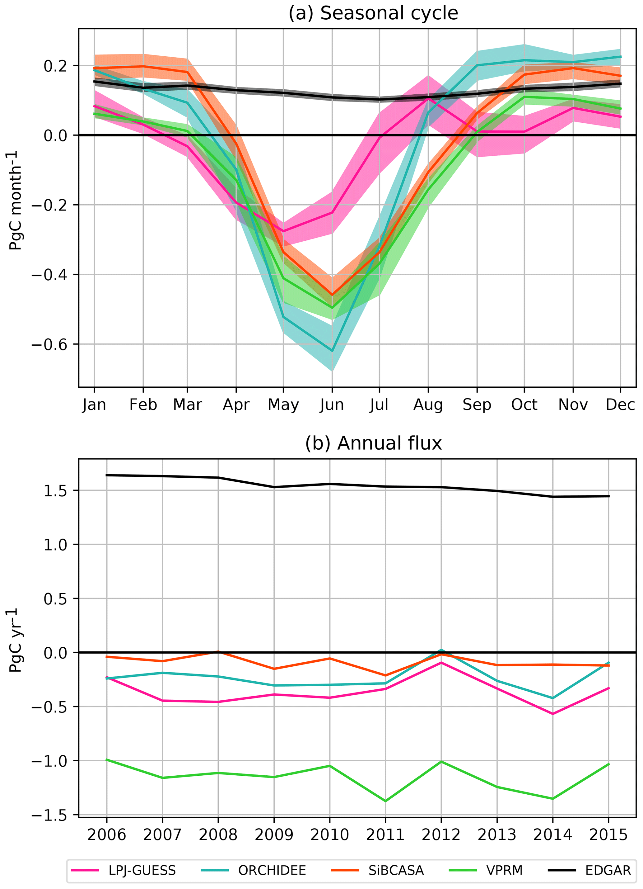
Figure 2 Seasonal cycle (a) and inter-annual variability (b) of the prior NEE (coloured lines/shading) and prescribed anthropogenic flux (black) used in the inversions, for geographical Europe (see definition in Sect. 3). The solid lines in the upper plot represents the mean seasonal cycle over the 10 years of the study, while the shaded envelopes show the minimum and maximum values over the same period.

3.2.2 Anthropogenic emissions

The anthropogenic emissions from combustion of fossil fuels and biofuels and from cement production are based on a pre-release of the EDGARv4.3 inventory for the base year 2010 (Janssens-Maenhout et al., 2019) and were provided as a 0.5^∘, hourly resolution product. This specific dataset includes additional information on the fuel mix per emission sector (Janssens-Maenhout, personal communication, 2017) and thus allows for a temporal scaling of the gridded annual emissions for individual years (2006–2015) according to year-to-year changes of fuel consumption data at national level (BP, 2016), following the approach of Steinbach et al. (2011). A further temporal disaggregation into hourly emissions is based on specific temporal factors (seasonal, weekly and daily cycles) for different emission sectors (Denier van der Gon et al., 2011). The seasonality and inter-annual variability of this anthropogenic emissions prior are also reported in Fig. 2 (in black).

Agricultural waste burning is already included in the version of the EDGAR v4.3 anthropogenic emission inventory that we are using. Also, large-scale biomass burning emissions are negligible in Europe (of the order of 0.01 Pg C yr⁻¹), and therefore we decided that no extra biomass burning emission dataset should be used in the inversions. Nevertheless, two models (LUMIA and FLEXINVERT) included a prescribed biomass burning source, based on the Global Fire Emission Database v4 (Giglio et al., 2013).

3.2.3 Ocean fluxes

The role of the ocean flux in causing spatial CO₂ gradients between stations at the European scale is very minor in regard to the magnitude of other fluxes (below −0.1 Pg C yr⁻¹). Therefore modelling groups were free to choose which ocean fluxes to use.

Two groups (LUMIA and FLEXINVERT+) used ocean fluxes from the CarboScope surface-ocean pCO₂ interpolation (oc_v1.6 and oc_v1.4 respectively) (Rödenbeck et al., 2013). The CarboScope interpolation provides temporally and spatially resolved estimates of the global sea–air CO₂ flux. Fluxes are estimated by fitting a simple data-driven diagnostic model of ocean mixed-layer biogeochemistry to surface-ocean CO₂ partial pressure data from the SOCAT database. NAME-HB used a climatological prior from Takahashi et al. (2009), which is based on a climatology of surface ocean pCO₂ constructed using measurements taken between 1970 and 2008. The CarboScope-Regional inversion used an ocean flux estimate taken from the Mikaloff Fletcher et al. (2007) global oceanic air–sea CO₂ inversion and CarbonTracker Europe optimized prior fluxes from the ocean inversion of Jacobson et al. (2007). Finally, PYVAR-CHIMERE used a null ocean prior but allowed the inversion to adjust it.

3.3 Inversion systems

The six inversion systems encompass a wide range of mesoscale regional transport models (with both Lagrangian and Eulerian models) and of approaches for the inversion (variational, ensemble and MCMC methods). The systems also differ by the definition of the boundary conditions, the selection of the observations to be assimilated, the definition of the control vector and the parameterization of uncertainty covariance matrices. Table 2 presents an overview of the participating systems characteristics.

Broquet et al. (2011)Fortems-Cheiney et al.Monteil and ScholzeThompson and StohlKountouris et al. (2018a)Peters et al. (2010)van der Laan-Luijkx et al. (2017)White et al. (2019b)(Cullen, 1993)(Rödenbeck et al., 2013)(Rödenbeck et al., 2013)Mikaloff Fletcher et al.(Jacobson et al., 2007)(Takahashi et al., 2009)

Table 2 Overview of the inverse modelling systems and configuration of the inversions.

^∗ The classification of low and high altitude varies on a case-by-case basis in some systems; see Fig. S2 for more information.

3.3.1 Transport models and boundary conditions

The six systems cover a diversity of models and model set-ups. Two systems (PYVAR-CHIMERE and CTE) rely on Eulerian transport models. The atmosphere is represented by a 3D grid (latitude, longitude and height). The CO₂ concentration is defined at each grid point and is altered at each time step by the CO₂ sources and sinks (i.e. the inversion control vector) in the surface layer, and by the air mass exchanges between the grid cells (at all layers). The other systems (LUMIA, FLEXINVERT, CarboScope-Regional and NAME-HB) all rely on Lagrangian transport models. In these systems, a Lagrangian transport model is used to compute, for each observation, a response function (footprint), i.e. a Jacobian matrix containing the sensitivity of the observed concentration to surface fluxes. The change in CO₂ concentrations resulting from the surface fluxes are simply the dot product of each footprint by the corresponding (slice of) the flux vector.

Beyond the Lagrangian/Eulerian distinction, the models differ by the underlying meteorological data used, and by the domain extent:

• The CHIMERE model (used in the PYVAR-CHIMERE system) is a regional Eulerian Chemistry transport model (Menut et al., 2013), forced with ECMWF operational forecasts. The simulations are performed at a horizontal resolution of 0.5^∘ and with 29 vertical levels up to 300 hPa, for the exact EUROCOM domain (as described at the beginning of Sect. 3).

• The CTE inversion relies on the global Eulerian transport model TM5 (Huijnen et al., 2010), driven by air mass transport from the ECMWF ERA-Interim reanalysis. TM5 is here run at a global resolution of $\mathrm{3}{}^{\circ }\times \mathrm{2}{}^{\circ }$, with a nested $\mathrm{1}{}^{\circ }\times \mathrm{1}{}^{\circ }$ zoom over Europe (12–66^∘ N, 21^∘ W–39^∘ E), and 25 vertical sigma-pressure levels.

• The CarboScope-Regional system (Kountouris et al., 2018a) relies on footprints from the STILT model (Lin et al., 2003). STILT footprints are computed for the exact EUROCOM domain, at a horizontal resolution of 0.25^∘, and at hourly temporal resolution, and they cover a period of 10 d prior to each observation. STILT is driven by short-term forecasts of the ECMWF-IFS model at 0.25^∘ resolution. The surface layer (up to which surface fluxes are mixed instantaneously) is defined as half the height of the planetary boundary layer, at any given time.

• In LUMIA, footprints covering the EUROCOM domain at a 0.5^∘, 3-hourly resolution were generated with the FLEXPART 10.0 model (Pisso et al., 2019), driven by ECMWF ERA-Interim meteorology. The footprints cover a period of 7 d prior to each observation and the surface layer is defined as the atmosphere below 100 m a.g.l.

• The FLEXINVERT inversion (Thompson and Stohl, 2014) also relies on footprints from the FLEXPART model, but driven by ECMWF operational forecasts. In contrast to CarboScope-Regional and LUMIA, the footprints are computed globally, on a 0.5^∘ hourly grid, and cover a period of 5 d before each observation.

• The NAME-HB system (White et al., 2019b) uses footprints from the NAME Lagrangian particle dispersion model. NAME is driven by 3-hourly meteorology from the UK Met Office's Unified Model (Cullen, 1993), at a spatial resolution which changes in time of 0.233^∘ latitude by 0.352^∘ longitude before mid-2014. The footprints are defined on a large regional domain, ranging from 10.729^∘ N, 97.9^∘ W to 79.057^∘ N, 39.38^∘ E with a spatial resolution of $\mathrm{0.233}{}^{\circ }\times \mathrm{0.352}{}^{\circ }$ (it covers the eastern half of North America, Europe and the northern half of Africa). The footprints are computed for a period of 30 d before each observation, at a 2-hourly temporal resolution in the first 24 h, and the remaining 29 d are integrated. The surface layer is defined as the layer below a height of 40 m.

Except for CTE which relies on a global model (although it runs at a very coarse resolution outside Europe), and all the other systems need boundary conditions (also called background concentrations), which represent the contribution of fluxes outside the space–time domain of the simulation:

• In PYVAR-CHIMERE and in NAME-HB, the background concentration (BCs) correspond to the transport of a boundary condition defined at the edge of the domain, by the transport model used in the inversion. In PYVAR-CHIMERE, the boundary condition is provided by a CAMS global inversion (Chevallier et al., 2010) and in NAME-HB it is derived from a global CO₂ simulation with the MOZART transport model (Palmer et al., 2018) (sampled at the time when and location where the NAME trajectories leave the NAME domain).

• CarboScope Regional and LUMIA both implement the two-step approach described in Rödenbeck et al. (2009). In short, the background concentrations correspond to the transport to the observation points of a boundary condition, taken from a global, coarse-resolution inversion, by the global transport model used in that global inversion. CarboScope-Regional relies on TM3 for its global inversion, and LUMIA relies on the TM5-4DVAR model.

• In FLEXINVERT, the footprints are global, therefore the background (from the perspective of the transport model) results only from the transport to the observation sites of the initial CO₂ distribution (i.e. the CO₂ distribution at the start of the period covered by each footprint). This initial concentration is calculated as a weighted average of a global CO₂ distribution sampled where and when the FLEXPART trajectories are terminated, and this global CO₂ distribution is based on a bivariate interpolation of observed CO₂ mixing ratios from NOAA sites globally, with monthly resolved fields. Note that for this system, the domain of the transport model is larger than that of the inversion itself.

The boundary conditions are specific to each system: from a technical point of view, the differences in domain extent and in the types of couplings with the boundary or background would make it hard to impose a common BC, but also, the boundary condition is an uncertain term: allowing a diversity of implementations is a way to maximize the exploration of the uncertainties in our intercomparison.

3.3.2 Inversion approaches

Four out of the six systems (PYVAR-CHIMERE, LUMIA, CarboScope-Regional and FLEXINVERT+) implement a variational inversion approach, in which the minimum of the cost function J(x) (Eq. 1) is searched for iteratively. The CTE inversion (Peters et al., 2007; van der Laan-Luijkx et al., 2017) employs an ensemble Kalman smoother with 150 members and a 5-week fixed-lag assimilation window. The NAME-HB inversion uses the MCMC method (Rigby et al., 2011; Ganesan et al., 2014; Lunt et al., 2016; White et al., 2019b). In short, this method samples the parameter space, and proposals for parameter values are accepted or rejected according to some rules based on the likelihood of the proposal.

Regardless of the inversion technique used, all the groups were asked to provide optimized NEE fluxes at a monthly, 0.5^∘ resolution on the EUROCOM domain. However, the precise control vector optimized in some of the inversions differ from this requested product:

• In PYVAR-CHIMERE, the NEE is optimized at a 6-hourly resolution on each grid cell (on the standard EUROCOM grid), starting from a prior NEE estimate from the ORCHIDEE model (See Sect. 3.2.1). In addition, the inversion also adjusts the ocean flux estimate, starting from a null prior. The prior uncertainty for each control vector element is proportional to the respiration in the corresponding grid cell (according to the same ORCHIDEE simulation) and further scaled to obtain an average uncertainty at the 0.5^∘ and 1 d scale of 2.27 µmol CO₂ m⁻² s⁻¹ (after Kountouris et al., 2018b).

• The LUMIA inversion controls the NEE fluxes monthly, on the standard EUROCOM grid, starting from prior NEE from the LPJ-GUESS model. The prior uncertainty is set to 50 % of the prior control vector (i.e. the prior NEE), with a minimum uncertainty set to 1 % of the grid point with the largest uncertainty, to avoid zero-uncertainty when NEE is close to zero. The decadal inversion was decomposed in 10 14-month inversions, from which the first and last month were not used.

• In the CarboScope-Regional system, the NEE fluxes are optimized every 3 h at a 0.5^∘ resolution in the EUROCOM domain, based on a prior NEE estimate from the VPRM model. The uncertainty of the prior NEE is set to a uniform value of 2.27 µmol CO₂ m⁻² s⁻¹, using a spatial error structure with a hyperbolic correlation shape. The set-up is identical to the “nBVH/” case in Kountouris et al. (2018a). The decadal inversion period was divided into three periods (2006–2007, 2008–2011 and 2012–2015).

• FLEXINVERT+ controls the NEE per country × plant functional type (116 control variables per time step across Europe, with PFTs based on those in the CLM model). The fluxes are optimized for 6-hourly periods (00:00–06:00, 06:00–12:00, 12:00–18:00, 18:00–00:00 local time, LT), averaged over 5 d. The prior NEE flux is based on the ORCHIDEE simulation described in Sect. 3.2.1, and the uncertainties are set proportional to this prior NEE. The transport model in FLEXINVERT+ is global, therefore the flux estimates used in the inversions are defined over the entire globe. However, the inversion only adjusts NEE within the EUROCOM domain.

• In NAME-HB, the domain of NAME has been split into eight boxes: four “background” boxes outside the EUROCOM domain, and four “foreground” boxes within the EUROCOM domain. The latter were further divided based on a PFT map used in the JULES vegetation model (Still et al., 2009), which includes six PFTs. The inversion optimizes separately the gross primary production (GPP, i.e. the uptake of carbon by plants) and the heterotrophic respiration (TER, with NEE = GPP + TER). The flux components are optimized at a variable temporal resolution, with a maximum resolution of 1 d (see White et al., 2019b, for further details). The oceanic flux is prescribed (based on the Takahashi et al., 2009, climatological pCO₂ estimate), but the background concentrations are part of the control vector and are therefore adjusted during the inversion. Therefore, there are 56 elements in the control vector, 4 elements to optimize the background concentrations, 4×2 elements to optimize the “background” regions for each of GPP and TER, 4×5 elements for the PFT regions for GPP (as one of the six PFTs is not applicable to GPP) and finally 4×6 elements for the PFT regions for TER. The uncertainties are set to 100 % of the prior for GPP and TER, and to 3 % of the initial value for the background terms.

• in CTE, the NEE and ocean fluxes are optimized globally on a weekly time resolution in a 5-week lagged window. The global domain is split into 11 TRANSCOM regions, which are further decomposed in ecoregions corresponding to 19 ecosystem types. The fluxes are optimized on $\mathrm{1}{}^{\circ }\times \mathrm{1}{}^{\circ }$ resolution for the Northern Hemisphere land regions, and by ecoregion and ocean region for the rest of the world. The prior NEE is taken from the SiBCASA simulation described in Sect. 3.2.1, and the prior oceanic flux is based on Jacobson et al. (2007).

In the three systems that optimize NEE at the pixel scale (LUMIA, PYVAR-CHIMERE and CarboScope-Regional), the spatial resolution of the control vector is in practice further limited by the use of distance-based spatial and temporal covariances in the flux covariance matrices (B in Eq. 1), which in effect smoothes the results by preventing the inversion from adjusting neighbouring pixels totally independently. The values of 100 km (CarboScope-Regional) and 200 km (PYVAR-CHIMERE and LUMIA) used for the spatial covariance lengths correspond well to the diagnostics of comparisons between the ecosystem simulations and flux eddy covariance measurements (Kountouris et al., 2018a). These systems and FLEXINVERT+ also assume temporal error covariances of 1 month at each grid cell.

The NAME-HB and FLEXINVERT+ inversions only control a limited number of PFTs in each region, which means that pixels in the same region and corresponding to the same PFT have a correlation coefficient of 1. Finally, CTE follows an intermediate approach. The flux uncertainties of Northern Hemisphere land pixels within a same ecoregion are correlated with a variable spatial covariance length to reflect the observation network density (200 km in Europe), and the uncertainties of grid boxes corresponding to different ecoregions are assumed to be uncorrelated. For the rest of the world, the uncertainties are coupled within each TRANSCOM region, decreasing exponentially with distance. The chosen prior standard deviation is 80 % on land parameters and 40 % on ocean parameters (van der Laan-Luijkx et al., 2017).

3.3.3 Observation vectors and errors

All the inversions use observations from the stations listed in Table 1. Each participant was, however, free to refine their selection of observations (both in terms of the number of sites assimilated and of data selection at each site) to adapt it to the skills of their own inversion system. In practice, five of the six inversions used data from nearly all the observation sites. NAME-HB used only a restricted list of 15 sites (see Fig. S1).

Most of the systems assimilate instantaneous or 1 h averages of the measurements, taken, when there are several vertical levels of measurements, at the top level of the stations, as it is the least sensitive to very local surface fluxes. NAME-HB assimilates 2-hourly observations (average of the observed concentrations in each 2-hourly interval). Due to the traditional limitations of transport models in terms of representation of the orography and simulation of the vertical mixing (Broquet et al., 2011), most of the systems use observations at low-altitude sites during the afternoon only, and observations at high-altitude sites during night-time only (vertical gradients of CO₂ near to the surface are notoriously difficult to simulate accurately, so observations when the vertical gradients are expected to be lower are preferred.)

• PYVAR-CHIMERE assimilates 1 h averages of the continuous or flask measurements over specific time windows that depend on the altitude of the stations above sea level. The selection window is 12:00–18:00 UTC time for stations below 1000 m a.s.l. and 00:00–06:00 LT for stations above 1000 m a.s.l. (following the analysis and choices by Broquet et al., 2011). The observation errors are set up as a function of stations, of the height of the station level above the ground and of the season, following the estimates by Broquet et al. (2011, 2013), based on comparison of simulations and measurements of radon. Their standard deviation for the 1 h averages ranges from 3 to 17 ppm.

• In LUMIA, observations from sites with continuous observations are selected based on the ``dataset_time_window_utc'' flag in the metadata of the observation files. That corresponds, for most sites, to a 11:00 to 15:00 UTC time range, and to a 23:00 to 03:00 UTC time range for mountain sites. At sites with only flask observations, all samples were used. The observation uncertainties are set as the quadratic sum of the measurement uncertainties, of the uncertainty associated with the foreground transport model (i.e. FLEXPART) and to the background concentrations. The measurement uncertainties are taken from the data files when available, and a minimum uncertainty of 0.3 ppm is enforced. Foreground transport model uncertainties are computed by performing two similar forward model runs, with TM5 and LUMIA (i.e. FLEXPART + background concentrations from TM5), configured such that the only difference is the model used to compute the transport within the EUROCOM domain (since the two models run at very different resolutions, this provides a reasonable proxy for the representation error). The uncertainties on the background concentrations are set as the standard deviation of the vertical profile of background CO₂ concentrations around each observation (see Monteil and Scholze, 2019, for details about the approach). Finally, a minimum value of 1 ppm was enforced for the combined uncertainty. On average, the combined uncertainty is of the order of 2 ppm (with site averages ranging from 1.02 for MHD to 4 ppm for PUI), but for individual observations it can be as high as 30 ppm.

• CarboScope-Regional assimilates observations, between 11:00 and 16:00 UTC for tall-towers, ground-based or coastal stations, and from 23:00 to 04:00 UTC for mountain stations (the time intervals refer to the beginning of the observation hour). A base representation error of 1.5 ppm was assumed for tall towers, coastal and mountain. For ground based continental sites it was raised to 2.0 ppm, and to 4 ppm for Heidelberg, which is in a urban environment. For sites that provide hourly observations, an error inflation was applied (e.g. for tall towers: 1.5 ppm $\times \sqrt{\text{6 obs per day}\times \text{7 day per week}}=\mathrm{9.7}$ ppm).

• In FLEXINVERT+, observations were assimilated hourly between 12:00 and 16:00 LT for sites below 1000 m a.s.l. and between 00:00 and 04:00 LT for sites higher than 1000 m a.s.l. The observation uncertainties are calculated as the quadratic sum of the measurement errors (with a minimum of 0.5 ppm), the uncertainty of the initial mixing ratio, assumed to be 1 ppm and the contribution of uncertainties in the fossil fuel emission estimates and in the NEE fluxes from outside the domain, both transported by FLEXPART to the observation sites. The total observation-space uncertainties typically range between 1 and 3 ppm.

• In NAME-HB, observations are filtered based on a combination of two metrics. One is the ratio of the NAME footprint magnitude in the 25 grid boxes closest to the measurement site. If this ratio is high it indicates that a large proportion of the air arriving at a measurement site is from very local sources and may not be resolved by the model. The second metric is the lapse rate modelled by NAME, which is the change of temperature with height and is a measure of atmospheric stability. A high lapse rate suggests very stable atmospheric conditions and may also indicate that there is a lot of local influence on the measurement. With these criteria, some data outside the usual daytime time constraints can be included and daytime data that are not collected during favourable conditions can be removed. In practice, however, most of the data included are measured during the daytime. The measurement uncertainties are taken from the data providers and averaged over the month for each measurement site to give a fixed monthly value. The observation uncertainty is adjusted during the inversion but initially it is the sum of the average measurement uncertainty and a model uncertainty of 3 ppm.

• In CarbonTracker-Europe, flags from data providers are used to screen for representative observations (usually equivalent to the afternoon hours for typical sites and night-time hours for mountain sites). A model–data mismatch based on the station category (tower, flask, etc.) is assigned to each site, accounting for both measurement errors and modelling errors at that site. If the difference between the forecast and observation is greater than 3 times that assigned model–data mismatch, the observations is not used in the inversion.

The range of uncertainties varies a lot across the systems and can range from one up to tens of parts per million. It reflects the different types of coupling between global and regional transport models, and the different range of diagnostics available for each group to quantify their uncertainties. The precise impact of these differences in prescribed observation uncertainties will be analysed in a follow-up study.

4 Results

4.1 Fit to the observations

Before presenting the posterior NEE, we first briefly analyse the misfits to the CO₂ observations assimilated by each inversion. The aims are to check that all inversions actually improve the model fits to the observations (which is a basic diagnostic of atmospheric inversions) but also to determine whether some sites are particularly problematic for some or all of the inversions.

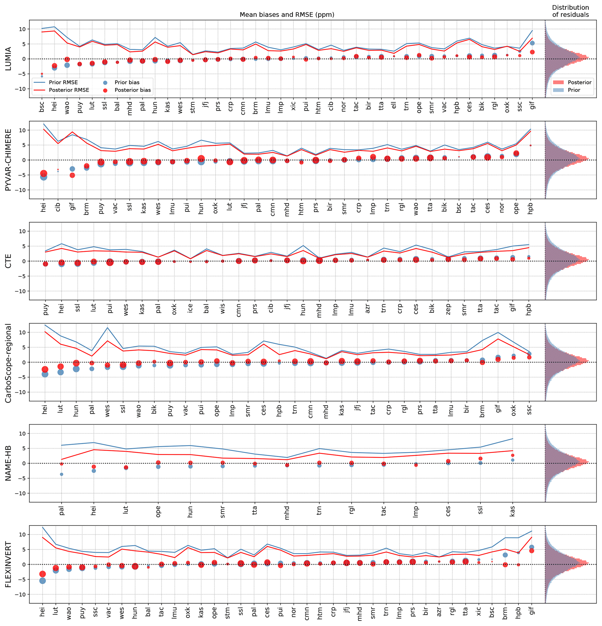
Figure 3 Prior (blue) and posterior (red) mean bias (dots) and RMSE (solid lines) at each observation site, for each inversion. The size of the dots is proportional to the number of assimilated observations. The histograms at the right of each subplot show the prior and posterior distribution of fit residuals for the entire ensembles of assimilated observations.

Comparisons between the prior and posterior bias and root mean square (RMS) differences (denoted RMS errors, i.e. RMSE) between the time series of measured and simulated data are shown for each inversion in Fig. 3, for each site (sorted according to the prior bias, for each inversion) and for the whole ensemble of assimilated observations. The expectation in this analysis is that all the systems should show a reduction of the misfits (both in terms of mean bias and RMSE). Ideally the posterior misfits should also be close to unbiased (i.e. with respect to the prescribed observational uncertainties).

All the inversions do indeed satisfy these expectations. The mean posterior biases range from −0.32 ppm (PYVAR-CHIMERE) to +0.04 ppm (NAME-HB). The largest bias reductions are obtained for the inversions that had the largest prior biases (CarboScope-Regional, with a mean bias reduced from −0.91 to −0.18 ppm, and NAME-HB, with a mean bias reduced from −0.87 to +0.04 ppm). The spread of the residuals is also reduced in all the inversions, with the strongest improvements obtained by NAME-HB (from 4.85 to 2.97 ppm), CarboScope-Regional (from 6.11 to 4.70 ppm) and FLEXINVERT (from 5.85 to 4.54 ppm). The best overall posterior fit is, however, obtained by CTE, with a posterior RMSE of 2.90 ppm and a posterior bias of +0.01 ppm.

The larger prior bias in CarboScope-Regional is easily explained by the substantially larger CO₂ sink of the VPRM prior (Sect. 3.2.1). On the contrary, NAME-HB uses the same ORCHIDEE prior as other inversions (PYVAR-CHIMERE, FLEXINVERT) so its prior bias must have a different origin (background, transport or oceanic flux). Note also that NAME-HB only covers a reduced 5-year period (2011–2015), which limits its comparability with the other inversions. The comparatively low RMSE obtained in the CTE inversion (including in the prior step), despite it using a lower-resolution transport model, shows that the resolution of the transport (and of the underlying meteorological data) is not the main limitation to fitting the observations.

At the site scale, the decrease in the misfits is rather moderate, up to 30 % but mostly below 20 %. Some sites tend to systematically be poorly fitted by the inversions (including in the posterior step), in particular those in the vicinity of large urban areas (with large anthropogenic emissions), such as HEI and GIF. Note that this is accounted for in several of the inversions, but not all, by inflating the model representation errors (which allows the model to degrade the fit to the observations, at a low “cost”). Besides these two sites, it does not appear that the distribution of the fits is systematic. In particular, there is no major difference between the fit to mountain-top (with night-time observations assimilated) and plain sites.

Table 3 Prior and posterior RMS difference (ppm) and percentage RMS difference reduction between modelled and observed concentrations, averaged hourly to annually. The average is first performed site by site, and then the site values are averaged together, with weights proportional to the length of each time series.

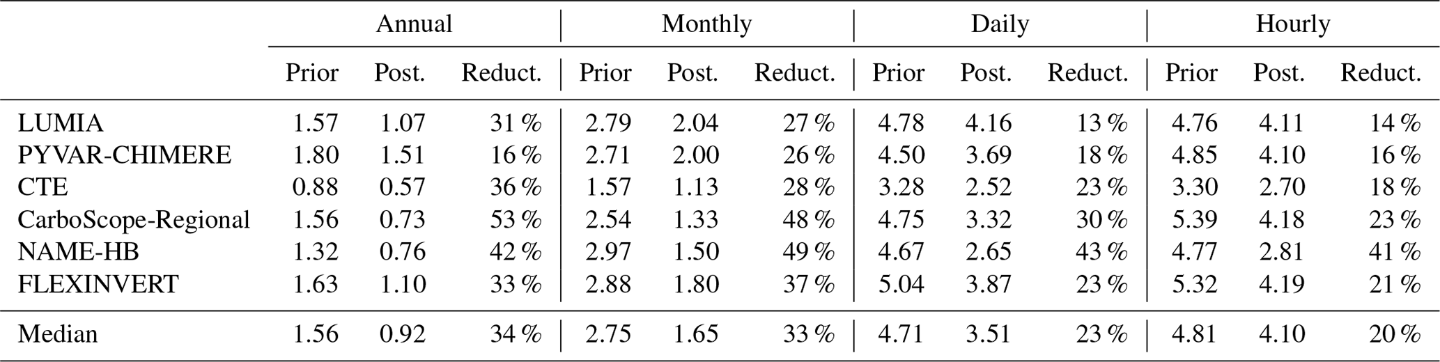
Error statistics computed on hourly to annual averages of the observations (Table 3) show considerably larger RMSE reduction for monthly and annual averages (respectively 33 % and 34 % ensemble median RMSE reduction) than for hourly and daily averages (20 % and 23 %, respectively). The only exception is NAME-HB, for which the error reduction is of the same order at all timescales (from 41 % for hourly averages to 49 % for monthly averages). This likely reflects the fact that, except for NAME-HB, all inversions use prior error covariance matrices implementing a temporal correlation length of 1 month between the flux adjustments, regardless of the actual temporal resolution of the inversions (see Table 2).

The monthly statistics are the most consistent across the ensemble (the larger error reduction obtained in CarboScope-Regional and NAME-HB are easily explained by their larger prior bias), which suggests that this is the temporal scale for which the comparison is the most robust.

This comparison of the residuals is an important technical diagnostic but does not indicate how realistic the posterior fluxes are and should not be interpreted as a ranking of the inversions. In particular, a good posterior representation of the observations is only a sign that the inversion had enough independent degrees of freedom to match the observed concentrations, but does not mean that the observations are sufficient to robustly constrain the control vector, or that the underlying transport model is accurate.

4.2 Posterior European-scale NEE

The monthly prior and posterior NEE values from the six inversions, integrated over the whole European domain (as defined in Sect. 3) and over the 10-year period of the intercomparison, are displayed in Fig. 4. The dominant feature in Fig. 4 is the systematic differences between the seasonal cycles; i.e. each inversion shows a similar pattern in the seasonal cycle (large/small amplitude or timing of peak values) for each year of the simulation period.

Figure 4 Monthly posterior fluxes, aggregated on the entire domain.

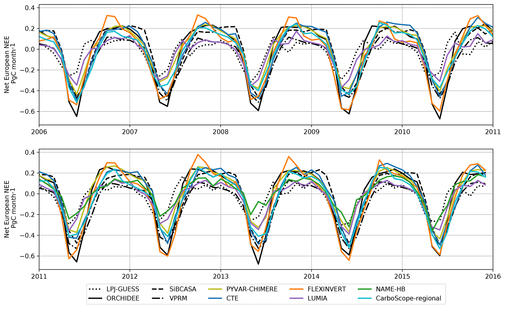
Overall, the posterior fluxes remain within or close to the range of values defined by the different priors. In Sect. 4.2.1 and 4.2.2, we compare the prior and posterior mean fluxes and their variability, at the annual and monthly timescales. In Sect. 4.2.3 we have a first look at the sub-continental scale. Results at the grid scale are provided for completeness in the Supplement but are not further discussed in this paper.

4.2.1 Long-term mean and variability of the annual NEE budget

Prior and posterior estimates of the annual budgets of the NEE over the European domain, as well as their mean and standard deviation over the inversion period, are reported in Fig. 5.

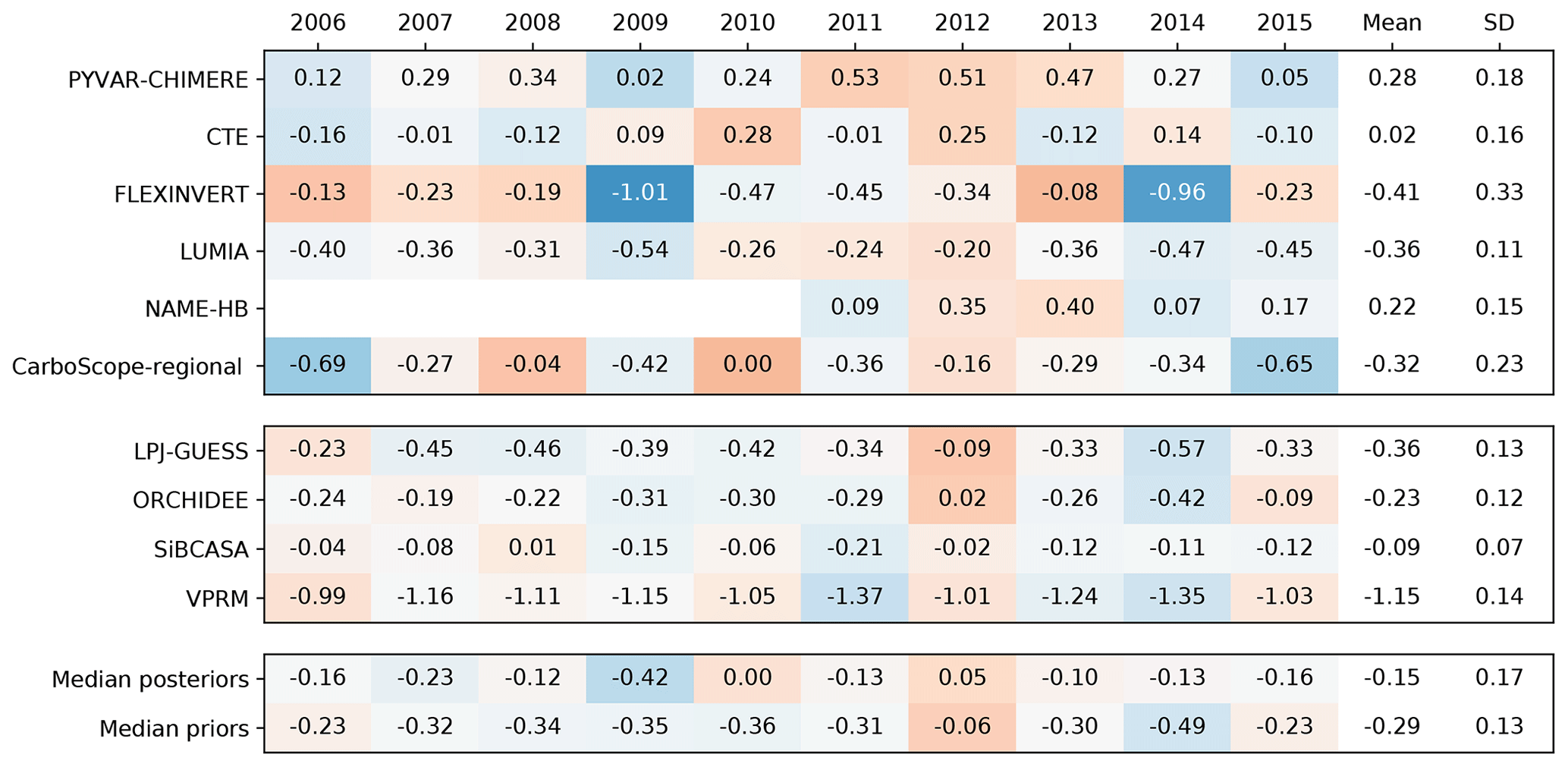
Figure 5 Annual NEE budget (positive for a source to the atmosphere and negative for a sink) for the six inversions (upper section of the array), for the four priors (middle section), and median prior and posterior fluxes (lower section). The two last columns show the mean NEE and the standard deviation of the NEE estimate, respectively, for each simulation. The colours of the cells indicate the strength and direction of the annual NEE anomaly (respective to the mean of each row; see Fig. 6 for the actual values).

We find an ensemble mean posterior estimate of the 10-year average NEE of −0.09 Pg C yr⁻¹ (−0.16 Pg C yr⁻¹ when excluding NAME-HB, which only covers the last 5 years), with values ranging from a net source of 0.28 Pg C yr⁻¹ (PYVAR-CHIMERE) to a net sink of −0.41 Pg C yr⁻¹ (FLEXINVERT). LUMIA and CarboScope-Regional estimate net sinks (−0.36 and −0.32 Pg C yr⁻¹, respectively) and the CTE inversion yields an almost neutral NEE budget (+0.02 Pg C yr⁻¹). Finally, besides PYVAR-CHIMERE, only the NAME-HB system finds the European ecosystems to be on average a net source of CO₂ to the atmosphere over our simulation period. Overall, the range of estimates from our inversions (0.7 Pg C yr⁻¹) is narrower than that of the priors (1.06 Pg C yr⁻¹ between VPRM and SiBCASA).

A large fraction of the average spread is due to systematic offsets between the optimized fluxes: the standard variation of the annual flux obtained in each inversion (taken as a metric for the inter-annual variability, IAV) is generally much smaller than the spread of the ensemble. The standard deviation of the annual NEE ranges from 0.11 Pg C yr⁻¹ (LUMIA) to 0.33 Pg C yr⁻¹ (FLEXINVERT), while the ensemble spread of the annual NEE is of the order of 0.8 Pg C yr⁻¹.

In the case of the CarboScope-Regional inversion, an obvious source for an offset from the other inversions is the prior flux from VPRM, which is much more negative than the other three priors. However, the differences between the three inversions using the NEE field from ORCHIDEE as a prior flux (PYVAR-CHIMERE, FLEXINVERT and NAME-HB) show that the biases between prior estimates can, at best, only partially explain the offsets in posterior estimates.

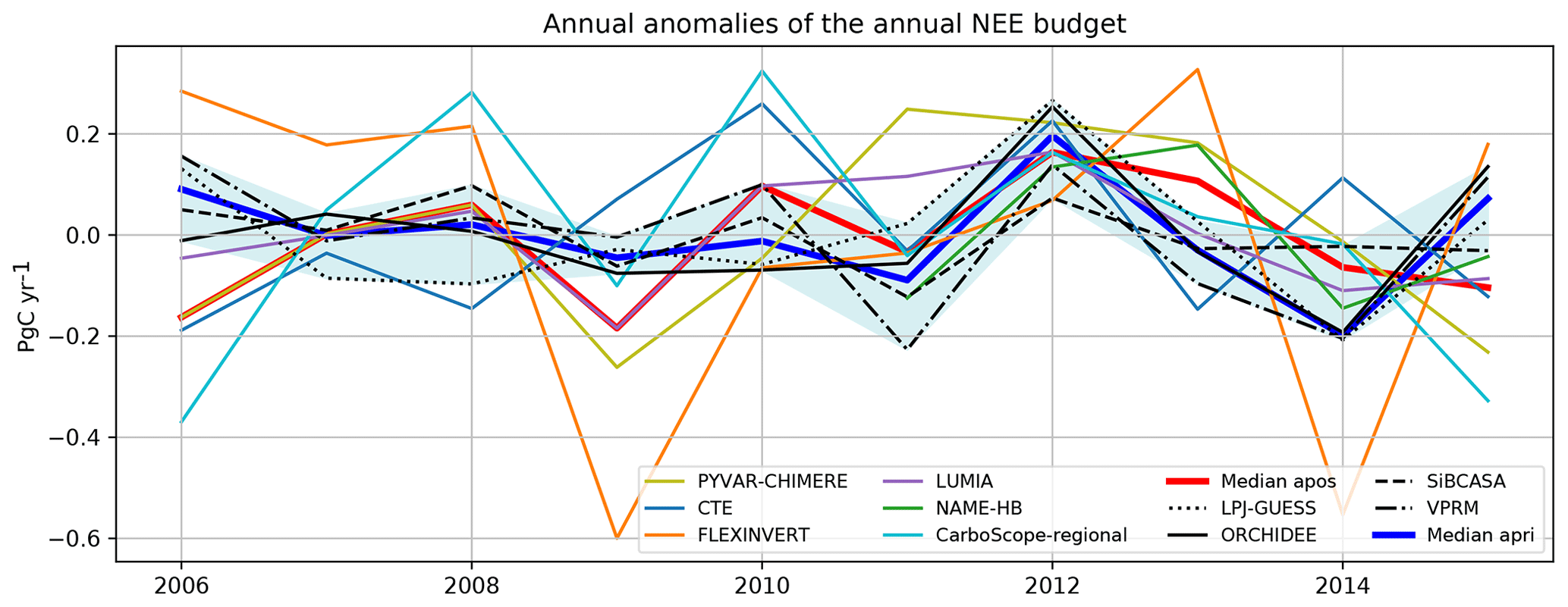
Figure 6 NEE anomalies of the six inversion posteriors and of the four priors. The median of the prior anomalies is shown as a thick blue solid line; that of the posteriors is shown as a thick red solid line. The blue shaded area shows the envelope of prior anomalies.

The annual anomalies of NEE are compared in Fig. 6, and the colours of the cells in Fig. 5 also scaled to these anomalies (with the long-term mean of each estimate taken as a reference). The ensemble spread of the posterior anomalies is generally much larger than that of the prior, although one system (FLEXINVERT) is contributing the most to such spread (in 2009 and 2014 for instance). The spread also strongly varies from year to year, from a minimum spread of 0.21 Pg C yr⁻¹ in 2007 to a maximum of 0.67 Pg C yr⁻¹ in 2009. In order to provide metrics less sensitive to potential model outliers, the medians of the prior (blue) and posterior (red) anomalies are shown in the Fig. 6.

There are a few consistent features, such as a clear positive anomaly in 2012, already present in the priors (median of +0.19 Pg C yr⁻¹) and further confirmed by the inversions (median value of +0.16 Pg C yr⁻¹). In contrast to the priors, however, the inversions point to a continuation of this anomaly in 2013 (+0.10 Pg C yr⁻¹) and do not confirm the negative anomaly present in most priors in 2014. The inversions also point to negative anomalies in 2006, 2009 and 2015 (respectively −0.16, −0.19 and −0.1 Pg C yr⁻¹) that are clearly outside the range of prior anomalies, although the spread of the ensemble is rather large for each of these three years (>0.5 Pg C yr⁻¹). Overall, however, the posterior median anomalies remain within or close to the range of prior anomalies for most of the 10-year period, but individual inversions can diverge a lot from the rest of the ensemble of posterior estimates, like FLEXINVERT before 2010 and in 2014.

In summary, the inversions clearly reduce the interval of estimates regarding the mean annual NEE of the European domain (compared to the ensemble of priors) but do not robustly capture the inter-annual variability of that annual flux. Analysing the differences in annual IAV is, however, complicated by the large spatial and temporal scales over which the fluxes are averaged: the observation network is not homogeneous, and the inversions may constrain some parts of the domain or times of the year better than others. In the following sections (Sect. 4.2.2 to 4.2.3) we analyse the inversion results at finer temporal and spatial scales.

4.2.2 Seasonal variability of NEE

The mean monthly posterior NEE estimates for the six inversions together with the prior fluxes are shown in Fig. 7. At first glance, the spread of the posterior fluxes approximately matches that of the prior estimations, with very similar mean spring (May–June) uptakes, ranging from −0.24 (NAME-HB) to −0.55 Pg C per month (FLEXINVERT) in the posteriors and from −0.28 to −0.62 Pg C per month in the priors. Winter posterior emissions are slightly higher (from +0.13 (LUMIA) to +0.32 Pg C per month in FLEXINVERT) than the priors (+0.11 to +0.23 Pg C per month). As a result, the median seasonal cycles are also very similar, with a similar phasing and a seasonal cycle amplitude of ≈0.55 Pg C.

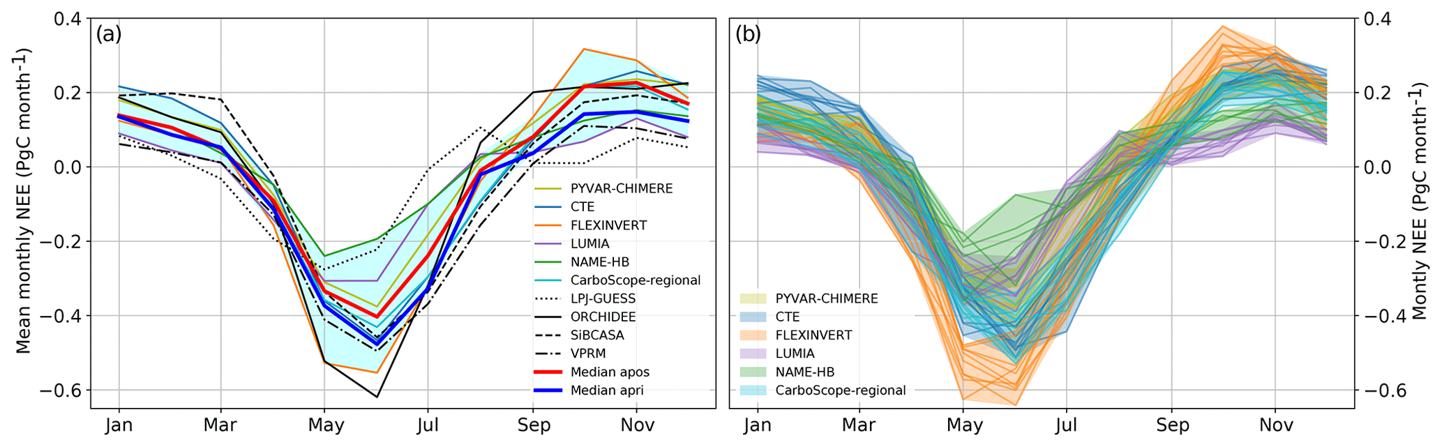
Figure 7 (a) Average seasonal cycles of the prior and posterior estimates. The prior and posterior ensemble median are represented as thick solid lines, and the spread of the posterior ensemble is shown as a shaded area. (b) Variability of the seasonal cycle during the 10 years of the inversion (the shaded areas represent the range of monthly NEE and the solid lines correspond to the individual years).

This similarity between the prior and posterior ensembles hides more significant differences at the level of individual ensemble members. The phasing of the seasonal cycle is very consistent among the inversions, with terrestrial ecosystems becoming a CO₂ sink (flux sign switch around April and August and with a peak uptake in June). On the contrary, the bottom-up simulations used as priors have four relatively distinct seasonal patterns (see also Fig. 2).

For instance, LPJ-GUESS simulates an early peak CO₂ uptake in May, which is not confirmed by the inversions (only NAME-HB yields to a similar peak). LPJ-GUESS simulates a NEE alternating between being a neutral flux and a positive but small (≈0.1 Pg C per month) net CO₂ source between July and March. This is most of the time outside or at the edge of the range of flux estimates derived from the inversions. The strong peak carbon uptake in June in ORCHIDEE (−0.62 Pg C per month in June) clearly exceeds the lower boundary of the posterior ensemble (−0.55 Pg C per month in FLEXINVERT). The positive NEE found by ORCHIDEE at the end of the summer (0.13 Pg C per month in August and September) is also contradicted by the inversions (≈0.04 Pg C per month ensemble median in these two months). The phasing of the seasonal cycles in VPRM and SiBCASA are in good agreement with that of the inversions. The winter NEE estimate in VPRM (≈0.07 Pg C per month between October and March) is lower than suggested by the inversions (ensemble median of 0.16 Pg C per month), and on the contrary, the inversions point to a lower NEE than found by SiBCASA in the first 3 months of the year (0.19 Pg C per month between January and March, compared to a corresponding ensemble median of 0.09 Pg C per month).

The variability of the seasonal cycles obtained with each system are illustrated in Fig. 7b. The systematic differences between the inversion systems dominate the picture and far exceed the monthly IAV within each inversion during the peak growth period (May–June) and during the autumn (October–November). The peak-to-peak amplitude of the mean seasonal cycle inferred by the different inversions varies between 0.4 Pg C per month for NAME-HB and 0.9 Pg C per month for FLEXINVERT.

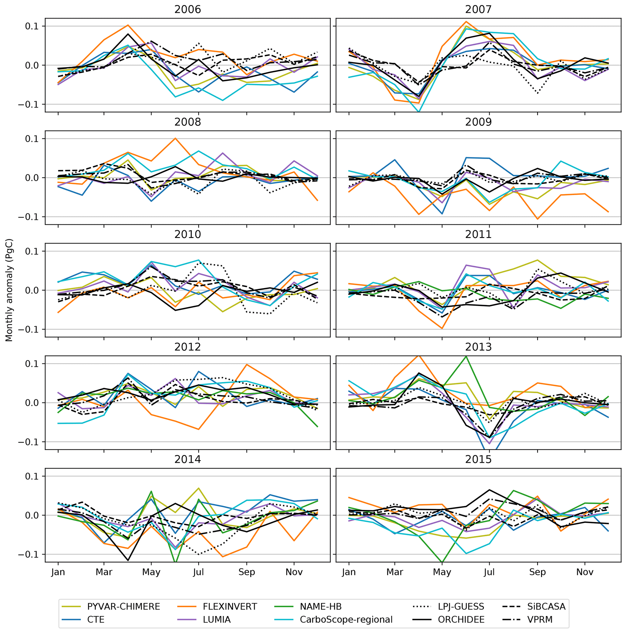
Figure 8 Monthly prior and posterior anomalies of the seasonal cycle, with each simulation compared to its own average seasonal cycle (Fig. 7a).

Figure 8 focuses on the monthly anomalies relative to the average seasonal cycle that drive these main differences. The figure provides more insights to explain the IAV of the annual budgets, discussed in Sect. 4.2.1. For instance, the negative annual flux anomaly (i.e. enhanced sink) found by four inversions in 2006 is explained by a stronger-than-usual carbon uptake in the summer of 2006. The negative NEE anomaly remains throughout most of the autumn and winter of 2006–2007 and becomes even more pronounced in March 2007, after which it switches sign. The 2012 anomaly is, on the contrary, spread over the entire year in almost all the inversions. It is, however, already well described by the priors, and the inversions here provide a confirmation.

In some instances it may be possible to relate these NEE anomalies to climate anomalies. For example, the summer 2006 in Europe was marked by a heatwave lasting for most of the month of July, and was followed by a particularly mild winter, which could explain the relatively stronger carbon sink from June 2006 to May 2007 (Rebetez et al., 2009). However, the size of our domain is assumedly much larger than the spatial extent of most potential climate anomalies, which complicates this type of analysis. We therefore briefly delve into the spatial distribution of the flux adjustments in the following section.

4.2.3 Spatial variability

Analysing the spatial variations of the fluxes may reveal robust local signals in areas where the transport models are more reliable and where the observation network is denser. It can also help to better interpret the results in terms of underlying processes in a large region such as Europe where the ecosystems and climate are highly heterogeneous. However, getting robust signals at regional scales is challenging due to the limited spatial resolution of the transport models and to the relative simplicity and large scales of the error correlations used for characterizing the prior flux uncertainties. A detailed analysis of the regional signals will be published in a follow-up article. Here, we only provide a brief overview of the spatial distribution of the NEE adjustments to provide a first assessment of the potential of regional inversions to analyse subcontinental-scale NEE variations and to support the previous analysis of the anomalies at the European scale.

We aggregate the fluxes in four large regions: northern Europe (Scandinavia, Finland and the Baltic states), southern Europe (the Iberian Peninsula, Italy, Greece, Romania and the Balkan states), western Europe (France, Benelux, the UK and Ireland) and central Europe (the remaining countries, up to the eastern border of Poland). The regions are pictured in Fig. 1. These four regions correspond roughly to four climate zones (Nordic, Mediterranean, oceanic and continental) and exclude parts at the edge of our domain which are not sampled by the observation network (North Africa, Turkey, far east of Europe).

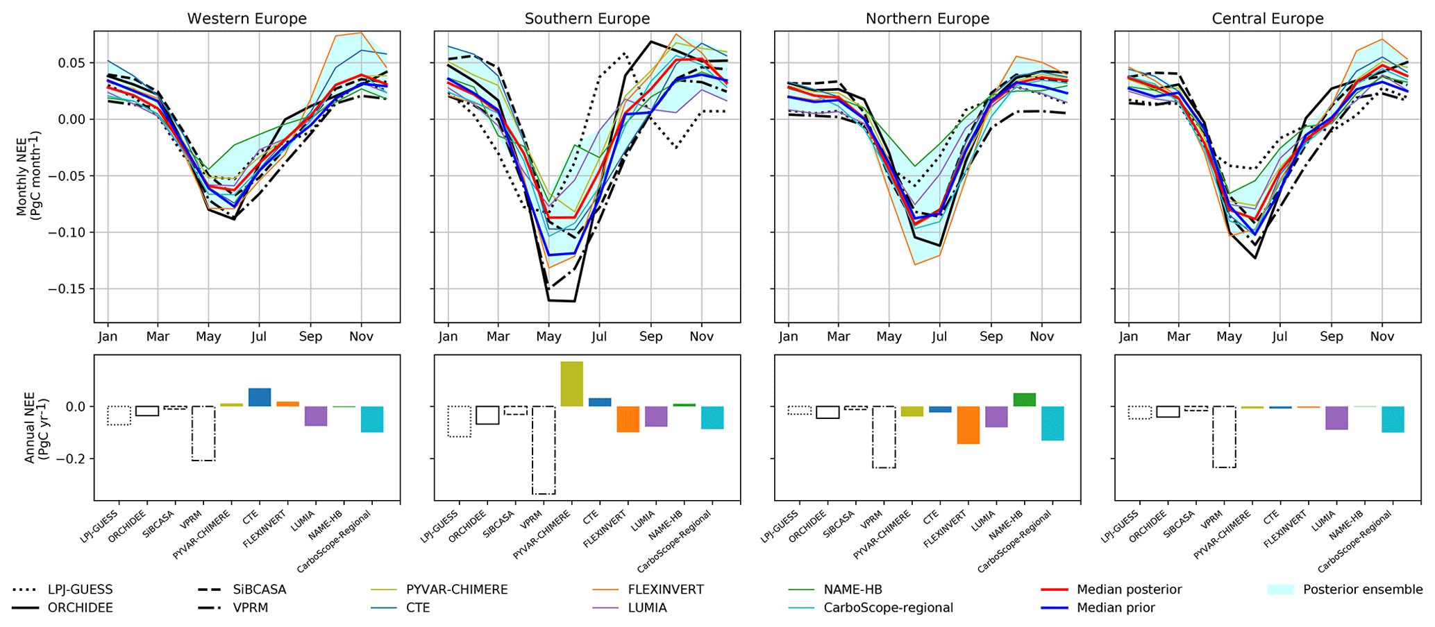
Figure 9 Upper row: mean prior (black lines) and posterior (coloured lines) seasonal cycle of the terrestrial carbon flux in the four regions highlighted in Fig. 1; prior and posterior ensemble median (thick blue and red lines) and posterior spread (blue shaded area). Lower row: mean annual net terrestrial carbon flux for these same regions.

Average regional monthly budgets for both prior and posterior estimates are shown for each region in the upper row of Fig. 9, along with the prior and posterior ensemble median and spread. Some of the systematic differences between the posterior seasonal cycles already noted at the European domain scale are present in all or most of the regions. This is in particular the case for the lower amplitude of the NAME-HB seasonal cycle and the positive autumn NEE peak in the FLEXINVERT inversion. But others, such as the positive bias of the PYVAR-CHIMERE posterior (i.e. 0.28 Pg C yr⁻¹; see Fig. 5), can be more clearly attributed to one specific region, like southern Europe.

Central Europe

NEE is most robustly estimated in the central Europe region, which is not surprising because it is the region most densely sampled by the observation network. The median prior and posterior fluxes are nearly identical, but the spread of the posterior ensemble is generally narrower than that of the prior fluxes. In particular, the LPJ-GUESS NEE estimate is clearly outside the range of posteriors in the summer (it points to a peak uptake of −0.04 Pg C per month in June, half of the −0.08 Pg C per month ensemble median).

In terms of net annual budget, the inversions fall in two categories: CarboScope-Regional and LUMIA point to a sink of −0.12 Pg C yr⁻¹, all the other inversion systems yield a close to zero annual budget. The similarity in the annual budget from these four inversions is, however, most likely by coincidence because the seasonal distribution of the fluxes is rather different (FLEXINVERT points to a summer uptake 30 % larger than that found in the NAME-HB inversion, compensated for by larger winter emissions).

Western Europe

Western Europe is also well sampled by the observation network, but because of the dominating westerly winds in our study domain, this region is more sensitive to boundary conditions than the central Europe region. The spread of the prior fluxes (0.02 to 0.04 Pg C per month) is narrower than in central Europe and is not further reduced by the inversions. In summer, the NAME-HB inversion suggests a reduced carbon uptake (−0.02 Pg C per month in June, compared to a prior ensemble mean of −0.06 Pg C per month), but as mentioned earlier, this is a systematic feature of that inversion, not specific to western Europe. In autumn (October to December), two inversions point to a much stronger positive flux than the priors and the other inversion systems (up to +0.75 Pg C per month in November, double the value of the posterior ensemble mean of +0.35 Pg C per month). As a result, there is little convergence between the annual budgets, which range between a net sink of −0.12 Pg C yr⁻¹ (CarboScope-Regional) and a source of 0.06 Pg C yr⁻¹ (CTE).

Southern Europe

The strongest corrections to the prior fluxes are obtained in southern Europe. The median value of the posterior estimates points to a ≈30 % reduction of the summer CO₂ uptake compared to the median of the prior fluxes. The spread of the posterior ensemble is larger than in the other regions (−0.08 to 0.14 Pg C per month) but this is also the region where the spread of the prior interval is the largest (up to 0.13 Pg C in July).

The shape of the LPJ-GUESS seasonal cycle is different from that of the other models, with two periods of negative NEE (February–June and October), and a peak carbon flux to the atmosphere in August. For most of the year, it remains outside the range of posterior scenarios and is therefore not compatible with the atmospheric observations.

The seasonal cycles of the three other prior fluxes are in phase with that of the inversion ensemble, but the amplitude of the summer uptake in ORCHIDEE and SiBCASA is larger than that inferred by the inversions, and the peak of carbon emissions simulated by ORCHIDEE in August and September is also corrected by the inversions (respectively 0.04 and 0.07 Pg C per month, compared to maximum ensemble posterior values of 0.02 and 0.04 Pg C per month).

Northern Europe

In northern Europe, for most of the year the range of posterior estimates is larger than that of the prior fluxes. All the simulations (including both prior and posterior) are well in phase, with a summer peak uptake in June–July and a stable winter flux between October and March. The inversions contradict the near-zero flux of the VPRM prior from August to December. The size of the summer uptake varies by a factor of 3, between the −0.04 Pg C per month as estimated by NAME in June and a corresponding value of −0.13 Pg C per month estimated by the FLEXINVERT inversion. The prior and posterior median are, however, nearly identical. Three inversions (CarboScope-Regional, FLEXINVERT and LUMIA) yield a clear annual net carbon sink (−0.06 to −0.14 Pg C yr⁻¹) for this region; however, the agreement on the size of the annual budget by CarboScope-Regional and FLEXINVERT is again by coincidence, as they distribute the fluxes very differently throughout the year.

5 Discussion

We have presented an overview of the results from the first set of inversions from the EUROCOM project. The ensemble includes one inversion for each of the participating systems and is designed so as to maximize the exploration of uncertainties, by covering a large diversity of inversion settings (prior, boundary condition, type of optimization technique and of optimized vector, etc.). This approach yields a more realistic approximation of the uncertainties and enables the dominant features of that uncertainty to be identified, better than what could be obtained from, for example, a set of sensitivity experiments using a single inversion system, or than the theoretical uncertainty estimates that are sometimes computed along with the inversions. The trade-off of that approach is that it does not easily permit the causes for the discrepancies between the inversions to be determined.

In the subsections below, we further discuss several aspects of our results, and put them in perspective with the previously published literature. First we discuss the annual budget of NEE in Europe, which has been a debated topic. Then in Sect. 5.2 we discuss the aspects of our results that are at this stage the most robust, and for which regional inversions seem the most relevant. Finally we briefly discuss the future perspectives of regional inversions, and of the EUROCOM intercomparison exercise.

5.1 How well can regional-scale inversions constrain the annual budget of European NEE?

The annual budget of NEE is a key metric to characterize the amount of carbon absorbed by the European ecosystems, since it balances the releases in winter and at night (by ecosystem respiration) with the uptakes during daytime, mostly in spring and summer (by photosynthesis). Annual to multi-annual budgets are an important measure to quantify the impact of environmental conditions such as ecosystem management, disturbances and climate extremes on the terrestrial carbon cycle.

The annual budget has notably been synthesized in Reuter et al. (2017): on the one hand, global inversions that assimilate only surface observations showed geographical Europe as a moderate to rather small carbon sink ($\approx -\mathrm{0.4}$ Pg C yr⁻¹) on multi-annual scales and, on the other hand, inversions constrained by satellite retrievals of total column atmospheric CO₂ (XCO₂) consistently infer that it is a much larger sink, of the order of −1 Pg C yr⁻¹. More recent studies suggest a smaller uptake: Scholze et al. (2019) find a mean sink of $-\mathrm{0.3}\pm \mathrm{0.08}$ Pg C yr⁻¹ by assimilating three datasets (namely in situ atmospheric CO₂ and remotely sensed soil moisture and vegetation optical depth) into their carbon cycle data assimilation system. Similarly, Crowell et al. (2019) estimate a mean sink of $-\mathrm{0.25}\pm \mathrm{0.46}$ Pg C yr⁻¹ from the ensemble of an intercomparison of atmospheric inversions based on XCO₂ observations from OCO-2. These estimates correspond to a geographical European domain which extends eastwards to the Urals, and which is much larger than the domain studied here. The areas of highest uptake in these satellite inversions are located in the eastern part of Europe, i.e. east of our EUROCOM domain.

From our ensemble of inversions we find a median sink of −0.15 Pg C yr⁻¹, relatively constant from year to year and with no significant trend over the 10 years of the period studied. Our study therefore tends to support the hypothesis that ecosystems in the European domain studied here are a weak carbon sink. Because of the differences in the domain extent, our inversions cannot close the controversy. But they indicate that, if there is a strong land sink over Europe (of the order of 1 Pg C yr⁻¹), then most of it has to be located in eastern Europe, beyond the extent of our dense observation network.

Figure 10 Comparison of the EUROCOM inversion ensemble with global inversions from the Global Carbon Project (Le Quéré et al., 2018). Panel (a) shows the annual NEE anomalies, with our prior and posterior ensembles shown as shaded areas, for the clarity of the figure. Panel (b) shows the mean annual budgets. The results from the global inversions were extracted for the exact EUROCOM domain on the global carbon atlas (http://www.globalcarbonatlas.org, last access: 6 August 2020).

Figure 10 provides results for our European domain (long-term mean and IAV) from a set of state-of-the-art global inversions that assimilate only surface observations and which cover the time period studied here. They correspond to the set of global inversions used for the Global Carbon Project annual analyses (Le Quéré et al., 2018). The range of mean annual NEE obtained from these global inversions is about half that obtained from our regional inversions (0.8 Pg C yr⁻¹), which suggests that, at this scale, our regional inversions do not constrain the annual NEE better than global inversions. The spread between these four state-of-the-art global inversions selected for the GCP synthesis actually corresponds to the outcome of a long process of improvement and selection of inversion configurations, as reflected by the very large spread of 1.8 Pg C yr⁻¹ obtained from the inter-comparisons by Peylin et al. (2013). Therefore, one can expect the process of inter-comparing regional-scale inversions started here with the EUROCOM project to yield a much-refined estimate of the annual to multi-annual budgets in the coming years.

The slightly narrower spread of the global inversions nonetheless questions specific aspects of the regional inversions, which may prevent them from providing more precise estimates of the continental-scale fluxes. Part of the constraint on the European NEE in global inversions comes from the observed large-scale atmospheric gradients between stations located in the Atlantic Ocean and Asia. These constraints are only incompletely transferred to regional inversion via their boundary conditions, and the shorter-scale gradients captured by the continental observations may not be sufficient to characterize the continental carbon balance. Unless the surface network is extended to sufficiently cover the eastern and southern parts of the domain, it might be useful to impose a constraint on the large-scale gradients to the regional inversions. However, this also means that the relevant scale for regional inversions is possibly much smaller. The next section thus focuses on the spatial and temporal scales where our ensemble of inversions leads to robust and consistent results.

5.2 New insights into the European land carbon flux

While the net annual carbon flux is an important metric, focusing on it can give an overly pessimistic view of the results, especially when integrated over the whole European domain, for which the observational coverage is not homogeneous. In fact, a large share of the discrepancies between the inversions can be attributed to regions located at the eastern and southern borders of our domain that are not part of the four regions discussed in Sect. 4.2.3 (Russia, Ukraine, Turkey and North Africa, but also large swathes of the “southern Europe” region).

Indeed, the ensemble of inversions leads to a narrower range of estimates than the ensemble of priors for regions with a dense network such as central Europe (0.21 Pg C yr⁻¹ of difference between the priors, vs. 0.10 Pg C yr⁻¹ between the posterior estimates). In contrast, the range of the ensemble of the inversions is almost 3 times the range of the prior estimates (0.33 Pg C yr⁻¹ between the optimized annual NEE, vs. 0.12 Pg C yr⁻¹ between the prior estimates) in the parts of the domain that are outside the four regions (see above), despite these regions being only rarely downwind of the observation network. This means that although the posterior annual estimates at the continental (whole-domain) scale may not be more robust than in the GCP global inversions, for example (as discussed in Sect. 5.1), the regional inversions in our intercomparison are capable of resolving annual fluxes at the scale of large countries (e.g. 0.8 to 1.6 million km² for the four regions defined in this paper), provided that the observational network is dense enough.

The size of the spread between the posterior monthly flux estimates varies by a factor of 5 throughout the year (at the continental scale). Monthly fluxes are usually well resolved in the first 9 months of the year except for June, but this larger spread in June is due to one single inversion (NAME-HB), which among other differences uses a much reduced observation network (See Sect. 4.1) and covers only the last 5 years of our simulation period. The larger range among the estimates at the end of the year is more problematic and points to a problem of the inversions to robustly resolve the winter NEE, i.e. the terrestrial respiration flux. Some speculative explanations could be larger systematic transport errors (winter concentrations are more difficult to represent, in particular at the highest latitudes, where the boundary layer remains extremely shallow, and the vertical atmospheric stratification is high when the days are very short) and/or larger relative differences in the prescribed prior flux uncertainties between the inversions (uncertainties are overall smaller in winter because of the lack of photosynthesis).

In three regions (western, central and northern Europe), the prior and posterior ensemble median of the seasonal cycle are almost identical, meaning that the inversions mostly provide a confirmation of the prior knowledge (see Fig. 9). However, the differences between our ensemble median (i.e. best-informed guess) and each individual prior are sometimes large. For instance, the inversions consistently yield a summer uptake twice as large in central Europe compared to the one computed by LPJ-GUESS. The results therefore present useful information for bottom-up modellers as they can be used to identify local or regional shortcomings in their models. This is also true when looking at the inversion results for southern Europe. Although the posterior estimates are not as consistent with each other as in the other regions, we nevertheless can clearly identify some shortcomings in the priors because they are far out of the ensemble spread (e.g. summer uptake by ORCHIDEE and SiBCASA, the double peak from LPJ-GUESS).

In summary, the relative lack of convergence of the annual fluxes at the scale of the continent hides more robust features at monthly and smaller regional scales, especially in central and western Europe, where the observation network is the densest. The divergences between the inversions regarding the winter fluxes will need to be investigated through a targeted effort. Nonetheless, the aim of optimizing fluxes at country scale appears achievable for the large countries in areas with a dense network. In recent years, the density of observation sites in northern Europe has increased a lot, so it is expected that the spread between the posterior estimates in this region can be reduced significantly in the future.

5.3 Future prospects of regional inversions and of the EUROCOM intercomparison

Our inversion protocol was intentionally very loose, to allow for the participation of a wide range of inversion systems and hence maximize the exploration of the space of uncertainties. It is therefore expected that the range of estimates would be large, and we consider it as a rather conservative representation of the actual uncertainties. The analysis of the results offers a few clues:

• The resolution of the transport model does not appear to be a major limitation (the best fit to the observations is actually obtained by the inversion using the lowest resolution transport model; see Table 3).

• Systematic patterns such as the differences in seasonal cycles or the average net annual NEE also seem relatively unaffected by the changes in the site selections that occur throughout the 10-year period, as the availability of data evolves (Fig. 7, right).

• The choice of a prior necessarily has an impact but can only explain a small fraction of the differences between the inversions (the differences between the three inversions using the ORCHIDEE prior are of the same order as the differences with the inversions using different priors).

The explanations for the spread of the ensemble are likely multi-factorial and specific to each feature of the spread. A traditional approach to assess the quality of inversion results would be to verify whether the posterior fluxes also enable improvements in the fit to independent (i.e. non-assimilated) observed CO₂ concentrations. This approach has, however, its own limitations. The goodness of fit to observations at one location cannot be generalized to the entire inversion domain or period. Using the few available (not already assimilated) concentration data (e.g. from aircraft measurement campaigns) could in fact deliver the incorrect message that one system is systematically over- or under-performing compared to the others. For the same reason, a validation by comparison with in situ flux measurements is risky, as the differences in scales between the fluxes optimized by the inversions and those measured by eddy-covariance sites, for example, are very large.

The inter-comparison exercise presented here does not enable a direct validation of the optimized fluxes, but it provides an estimation of how large the uncertainties are, and it helps identify its dominant features in a more systematic manner than what could be done with just one inversion system. To conclusively determine the drivers of that uncertainty and discriminate their relative contributions, targeted efforts will be needed, primarily in the form of sensitivity experiments using a stricter protocol and focusing on one driver of uncertainty at a time. The knowledge gained from the first phase of the intercomparison will help design these new experiments, which should rapidly lead to an improved convergence of the ensemble.

6 Conclusions and future of the EUROCOM project

The EUROCOM project delivered a set of European NEE estimates at a 0.5^∘, monthly resolution at the disposal of the scientific community (Monteil et al., 2020). The data can be used as a comparison and validation dataset for both bottom-up and inverse modellers. The input datasets (observations and prior fluxes) remain available for inverse modelling groups willing to submit additional inversions, and we expect the size and robustness of the ensemble to grow over time. An extension of the inversions until 2019 is currently ongoing.

Our best posterior estimate (ensemble median) of the long-term mean annual terrestrial European NEE of $-\mathrm{0.15}\pm \mathrm{0.08}$ Pg C yr⁻¹ over the years 2006–2015 is comparable to the median value of $-\mathrm{0.3}\pm \mathrm{0.11}$ Pg C yr⁻¹ from our prior estimates as well as recent estimates from other studies (e.g. Scholze et al., 2019; Crowell et al., 2019, albeit for a slightly different domain). Since our domain here does not cover the European part of Russia, the area that is postulated to contribute most to the large European carbon sink (see for example Reuter et al., 2017), we cannot resolve this controversy here with our intercomparison.

We deliberately kept the requirements in the intercomparison protocol (i.e. use of prescribed common datasets or inversion set-ups) to a minimum (namely, prescribed fossil fuel emissions and common domain) to encourage the participation of voluntary contributions from regional atmospheric inverse modelling groups. Such an intercomparison approach, where a large number of parameters influencing results of the inversions vary from one system to another, presents the advantage that the resulting distribution of results provides a good approximation of the distribution of uncertainties on the net European terrestrial carbon flux. Indeed, the analysis shows that no inversion is clearly more or less valid than the others, and, depending on the focus metrics, each can be an outlier. Such a multi-model and multi-inversion system ensemble is the best approach for providing robust estimates of the European carbon budget.

The most robustly modelled feature in our ensemble is the mean seasonality of the annual CO₂ sink in regions with a dense observational network, i.e. mainly central and western Europe, illustrating the usefulness of a coordinated infrastructure such as ICOS in delivering high-quality observations. The coverage of the observational network in some regions of Europe is still limited, which is clearly reflected in a larger spread in the annual and monthly budgets in these regions within our ensemble. Observations from satellites, such as OCO-2 or the upcoming CO2M, may help in increasing the coverage but they have their own limitations (prone to clouds and aerosols, limited coverage during the winter season if based on passive optical instruments).

The mean annual terrestrial NEE itself is not strongly constrained by the observations and we find a spread of 0.7 Pg C yr⁻¹ within our ensemble. As mentioned above, this is partly because of the high freedom in the choice of settings. This freedom in the choice of settings makes it rather challenging to fully understand the causes of the spread in the ensemble results and the underlying uncertainties. We will investigate these differences in more detail and evaluate some of the specific parameters involved in the inversion set-ups in a forthcoming paper. Eventually, this will lead to a much better quality of the regional inversion estimates that could not have been possible without such an intercomparison exercise.

Currently, the main benefit of regional inversions over global ones does not appear to be at the scale of the continent, but rather at finer spatial scales, in regions well covered by the observation networks. The observation network seems sufficiently dense to envision robust country-scale estimates of the carbon balance (at least for the largest countries) in western and central Europe. Recent expansions of the networks both in northern and southern Europe should also enable a significant reduction of the spread between the inversions in the near future.