Tropospheric ozone radiative forcing uncertainty due to pre-industrial fire and biogenic emissions

Tropospheric ozone concentrations are sensitive to natural emissions of precursor compounds. In contrast to existing assumptions, recent evidence indicates that terrestrial vegetation emissions in the pre-industrial era were larger than in the present day. We use a chemical transport model and a radiative transfer model to show that revised inventories of pre-industrial fire and biogenic emissions lead to an increase in simulated pre-industrial ozone concentrations, decreasing the estimated pre-industrial to present-day tropospheric ozone radiative forcing by up to 34 % (0.38 to 0.25 W m⁻²). We find that this change is sensitive to employing biomass burning and biogenic emissions inventories based on matching vegetation patterns, as the co-location of emission sources enhances the effect on ozone formation. Our forcing estimates are at the lower end of existing uncertainty range estimates (0.2–0.6 W m⁻²), without accounting for other sources of uncertainty. Thus, future work should focus on reassessing the uncertainty range of tropospheric ozone radiative forcing.

1 Introduction

Tropospheric ozone (O₃) is a short-lived greenhouse gas formed in the atmosphere through photochemical oxidation of volatile organic compounds (VOCs) in the presence of nitrogen oxides (NO_x). These precursor gases have both natural and anthropogenic sources, and increased anthropogenic emissions are thought to have caused an increase in global tropospheric O₃ of 25 %–50 % since 1900 (Gauss et al., 2006; Lamarque et al., 2010; Young et al., 2013). The Intergovernmental Panel on Climate Change (IPCC) current best estimate for tropospheric O₃ radiative forcing (RF) over the industrial era is 0.4±0.2 W m⁻² with a 5 %–95 % confidence interval, making tropospheric O₃ the third most important anthropogenic greenhouse gas after CO₂ and CH₄ (Myhre et al., 2013). The present-day (PD) radiative effect (RE) of tropospheric O₃ is relatively well constrained (Rap et al., 2015). The large uncertainty range (0.2–0.6 W m⁻²) is caused by a number of factors such as the radiative transfer scheme employed, the model used to simulate tropospheric O₃ and tropopause definition; however, it is primarily associated with a poor understanding of pre-industrial (PI) O₃ concentrations (Myhre et al., 2013; Stevenson et al., 2013). Although measurements of tropospheric O₃ exist as far back as the late 19th century, there are limited reliable quantitative measurements of tropospheric O₃ prior to the 1970s (Volz and Kley, 1988; Cooper et al., 2014). Recently, Checa-Garcia et al. (2018) found that differences in PI estimates between Coupled Model Intercomparison Project phase 5 (CMIP5) and CMIP6 cause an 8 %–12 % variation in O₃ RF estimates but did not explicitly assess uncertainty in natural PI emissions. Recent analysis of oxygen isotopes in polar ice cores indicates that tropospheric O₃ in the Northern Hemisphere increased by less than 40 % between 1850 and 2005, suggesting that O₃ RF may be lower than the 0.4 W m⁻² estimate (Yeung et al., 2019).

As well as anthropogenic sources, O₃ precursor gases such as methane (CH₄), carbon monoxide (CO) and NO_x have natural emission sources, e.g. wildfires, wetlands, lightning and biogenic emissions. Wildfires, for example, emit large quantities of CO, NO_x, CH₄ and non-methane volatile organic compounds (NMVOCs) (van der Werf et al., 2010; Voulgarakis and Field, 2015), which influence the chemical production of O₃ (Wild, 2007). Changes in the natural environment therefore influence the concentration and distribution of tropospheric O₃ (Monks et al., 2015; Hollaway et al., 2017). While human activities such as deforestation, land-use change and fire management are known to affect natural emission sources of O₃ precursor gases, their impact on emissions net change remains very uncertain (Mickley et al., 2001; Arneth et al., 2010). An accurate representation of PI natural emissions is therefore very important for quantifying the PI-to-PD tropospheric O₃ RF calculations.

Recent studies suggest that the relationship between humans and fire (Bowman et al., 2009) is more complex than previously assumed (Doerr and Santín, 2016). The expansion of agriculture and land-cover fragmentation since PI has decreased the abundance and continuity of fuel, inhibiting fire spread (Marlon et al., 2008; Swetnam et al., 2016) and hence total emissions. Furthermore, at the global scale, increased population density results in declining fire frequency (Knorr et al., 2014; Andela et al., 2017). Increased agricultural land coupled with active fire suppression and management policies mean that human activity has likely caused total fire emissions to decline since the PI (Daniau et al., 2012; Marlon et al., 2016; Hamilton et al., 2018). Paleoenvironmental archives of fire activity also reflect a decline of fire over the industrial era in many regions (Marlon et al., 2016; Rubino et al., 2016; Swetnam et al., 2016). This change in the understanding of PI fire emissions has been shown to have a strong influence on aerosol RF: Hamilton et al. (2018) estimated a 35 %–91 % decrease in global mean cloud albedo forcing over the industrial era when using revised PI fire emission inventories.

Emissions of biogenic VOCs (BVOCs), such as isoprene and monoterpenes, from vegetation also affect tropospheric O₃ formation. Isoprene contributes to the formation of peroxyacetylnitrate (PAN), which has a lifetime of several months in the upper troposphere (Singh, 1987), allowing long-range transport of reactive nitrogen and enhancing O₃ formation in remote regions. PAN formation is also highly dependent on NO_x concentrations, meaning that changes in the distribution of emissions and the magnitude will impact O₃ formation. Previous studies of PI tropospheric O₃ have often assumed that PI BVOC emissions were equivalent to or lower than those in PD (Stevenson et al., 2013). In Stevenson et al. (2013), only one model of the ensemble included PI isoprene emissions that were larger than in the PD simulation. However, BVOC emissions are sensitive to climate, CO₂ concentrations, vegetation type and foliage density, each of which has changed since the PI (Laothawornkitkul et al., 2009; Hantson et al., 2017) and needs to be accounted for when calculating O₃ RF.

The aim of this study is to examine the effect of revised PI fire and BVOC emission inventories on PI-to-PD tropospheric O₃ RF estimates. We use a global chemical transport model (CTM) and a radiative transfer model to investigate the impact of these revised natural PI emission inventories on tropospheric O₃ PI concentrations and its PI–PD RF. The IPCC 5th assessment report moved to the concept of effective radiative forcing (ERF) (Myhre et al., 2013) to more completely capture the expected global energy budget change from a given driver. However, here we employ the more traditional stratospherically adjusted RF as it can be estimated with more certainty than ERF, and previous studies suggest that ERF and RF are likely to be similar for O₃ change (Myhre et al., 2013; Shindell et al., 2013). We note that a number of factors not considered here also introduce uncertainty when simulating PI tropospheric O₃ concentrations, e.g. changes to lightning and soil NO_x emissions, O₃ deposition and atmospheric transport. However, the purpose of this study is to address and focus on the uncertainty associated with natural emissions in the pre-industrial era by utilising the revised inventories of fire and biogenic emissions.

2 Methods

2.1 TOMCAT–GLOMAP

We used the TOMCAT global three-dimensional offline chemical transport model (CTM) (Chipperfield, 2006) coupled to the GLOMAP modal aerosol microphysics scheme (Mann et al., 2010) to simulate tropospheric composition and its response to emissions changes. The model used a $\mathrm{2.8}{}^{\circ }\times \mathrm{2.8}{}^{\circ }$ horizontal resolution with 31 vertical levels from the surface to 10 hPa. All simulations were run with 6-hourly 2008 meteorology from European Centre for Medium-Range Weather Forecasts (ECMWF) ERA-Interim reanalyses with a 1-year spin-up (Dee et al., 2011). The model includes a detailed representation of hydrocarbon chemistry and isoprene oxidation, and it has previously been shown to accurately reproduce observed concentrations and distributions of key tropospheric species such as O₃, CO, NO_x and VOCs (Monks et al., 2017; Rowlinson et al., 2019). The annual global mean surface CH₄ mixing ratio is scaled in TOMCAT–GLOMAP based on observed global mean surface concentrations for the year being simulated; however, the spatial variation in CH₄ concentrations is maintained in the model. Biomass burning and biogenic emissions are emitted into the lowest model level, which extends from the surface to 951 hPa.

2.2 Radiative transfer model

Tropospheric O₃ RFs were calculated using the SOCRATES radiative transfer model (Edwards and Slingo, 1996) with six bands in the shortwave (SW) and nine in the longwave (LW). This version has been used extensively in conjunction with TOMCAT–GLOMAP for calculating O₃ radiative effects (Bekki et al., 2013; Rap et al., 2015; Kapadia et al., 2016; Scott et al., 2018). We used the fixed dynamical heating approximation (Fels et al., 1980) to account for stratospheric temperature adjustments, i.e. changes in the stratospheric heating rate calculated in the model due to the O₃ perturbation are applied to the temperature field, with the model run iteratively until stratospheric temperatures reach equilibrium (Forster and Shine, 1997; Rap et al., 2015).

2.3 Simulations

We investigate the effect of natural PI emissions on PI-to-PD changes in tropospheric O₃ concentrations by contrasting PI against PD model simulations (Table 1). All simulations are run with PD meteorology and global mean surface CH₄ concentrations scaled to be 722 ppb in the PI and 1789 ppb in PD (Etheridge et al., 1998; Dlugokencky et al., 2005; Hartmann et al., 2013; McNorton et al., 2016).

Table 1 Details of the TOMCAT–GLOMAP simulations performed in this study.

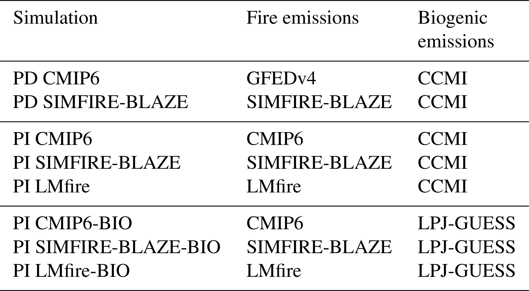
All PI simulations considered anthropogenic emissions set to zero, except for biofuel emissions taken from AeroCom for the year 1750 (Dentener et al., 2006). The first set of three PI simulations (i.e. PI CMIP6, PI SIMFIRE-BLAZE and PI LMfire) investigates the impact of fire emissions only by keeping BVOC emissions (i.e. isoprene and monoterpenes) at their PD values based on the Chemistry–Climate Model Initiative (CCMI) biogenic emissions (Sindelarova et al., 2014). The second set of three PI simulations (i.e. PI CMIP6-BIO, PI SIMFIRE-BLAZE-BIO and PI LMfire-BIO) investigates the additional impact of PI biogenic emissions by combining each PI fire emission inventory with an estimate of PI BVOC emissions from the LPJ-GUESS model (Arneth et al., 2007; Schurgers et al., 2009; Smith et al., 2014).

The PD simulations used anthropogenic emissions from the MACCity emissions dataset (from EU projects MACC/CityZEN; Lamarque et al., 2010) and CCMI biogenic emissions (Sindelarova et al., 2014). Two PD simulations were performed, namely the primary PD simulation (PD CMIP) driven by the Global Fire Emissions Database version 4 with small fires (GFED v4s) inventory as employed in CMIP6 (Randerson et al., 2017; van Marle et al., 2017) and PD SIMFIRE-BLAZE (Knorr et al., 2014). A PD simulation is not available for LMfire, a PI fire model not designed to undertake a PD simulation. To isolate the effect of revised natural PI emissions on PI-to-PD tropospheric ozone RF, we compare the six PI simulations against the main PD CMIP6 simulation. The other PD simulation, i.e. PD SIMFIRE-BLAZE, is also included in our analysis in order to explore the additional uncertainty in RF introduced by PD emission inventories uncertainties. However, as PD tropospheric ozone RE was shown to be well constrained by satellite observations (Rap et al., 2015), this additional uncertainty is known to be small.

2.4 Fire emission inventories

Following Hamilton et al. (2018), we used three PI inventories to investigate the sensitivity of tropospheric O₃ RF to PI fire uncertainty. The CMIP6 PI inventory is treated as a control, as this has been widely used in previous studies and was developed from a set of global fire models, with SIMFIRE-BLAZE and LMfire providing PI perturbation scenarios from this baseline.

2.4.1 Pre-industrial and present-day CMIP6

CMIP6 provides monthly mean emissions of CO, NO_x, CH₄ and VOCs from fires. In the PD, CMIP6 emissions are derived from satellite estimates of global burden area and active fire detections (Randerson et al., 2012; Giglio et al., 2013). In the absence of satellite data, PI CMIP6 fire emissions are generated by merging PD satellite observations with fire proxy records, visibility records and analysis from six fire models (van Marle et al., 2017). The mean of 1750–1770 emissions is used in this study to represent PI emissions. Biomass burning emissions from deforestation and peat fires are assumed to be reduced in the PI, while agricultural fires are kept fairly constant with PD due to a lack of information on the PI environment.

2.4.2 Pre-industrial and present-day SIMFIRE-BLAZE

The SIMFIRE-BLAZE PI fire emission inventory was developed using the LPJ-GUESS-SIMFIRE-BLAZE model. The PI emissions employed here are the mean for the period 1750–1770 (Hamilton et al., 2018). The LPJ-GUESS dynamic vegetation model predicts ecosystem properties for given climate variables (Smith et al., 2014), which, combined with the HYDE 3.1 dataset of human land-use change, allows for the simulation of global PI land cover (Klein Goldewijk et al., 2011). The SIMple fire model (SIMFIRE) calculates total burned area (Knorr et al., 2014), with the total fire carbon flux calculated from BLAZE (BLAZe induced biosphere–atmosphere flux Estimator) (Rabin et al., 2017). Akagi et al. (2011) emissions factors were used with separate treatment of herbaceous and non-herbaceous as well as tropical and extratropical vegetation to produce emission inventories. Agricultural fire emissions are not included. Total PI fire emissions of gas species in the SIMFIRE-BLAZE inventory are 28 % larger than in the PI CMIP6 inventory.

The fire emissions in the PD SIMFIRE-BLAZE model are very similar to the PD CMIP6 inventory, with only slightly increased global NO_x emissions (174 Tg yr⁻¹ compared to 171  Tg yr⁻¹ in CMIP6) and CO emissions (1027  Tg yr⁻¹ compared to 970  Tg yr⁻¹). The global distribution of the inventories is also similar (Fig. 1), with slightly larger CO emissions in the SH tropics in PD SIMFIRE-BLAZE but smaller in the NH tropical region. NO_x and VOC emissions are similar in both inventories across all latitude bands (Fig. 1b, d). The seasonality of emissions is also consistent across both inventories in terms of NO_x and VOC emissions; however, for CO the peak in emissions is slightly later for the SIMFIRE-BLAZE inventory (Fig. 3). The slightly higher emissions in PD SIMFIRE-BLAZE result in a simulated tropospheric O₃ burden of 359.9 Tg, an increase of 1 % relative to the PD CMIP6 TOMCAT–GLOMAP simulation (Table 2).

Table 2 Annual mean global tropospheric burdens of CO, NO_x and O₃, mean tropospheric OH concentration, tropospheric column O₃ for all model simulations, and 1750–2010 radiative forcing of tropospheric O₃ estimated for each PI simulation against the PD CMIP6 simulation.

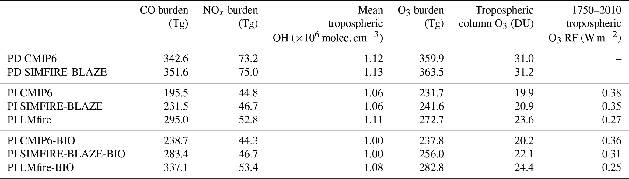
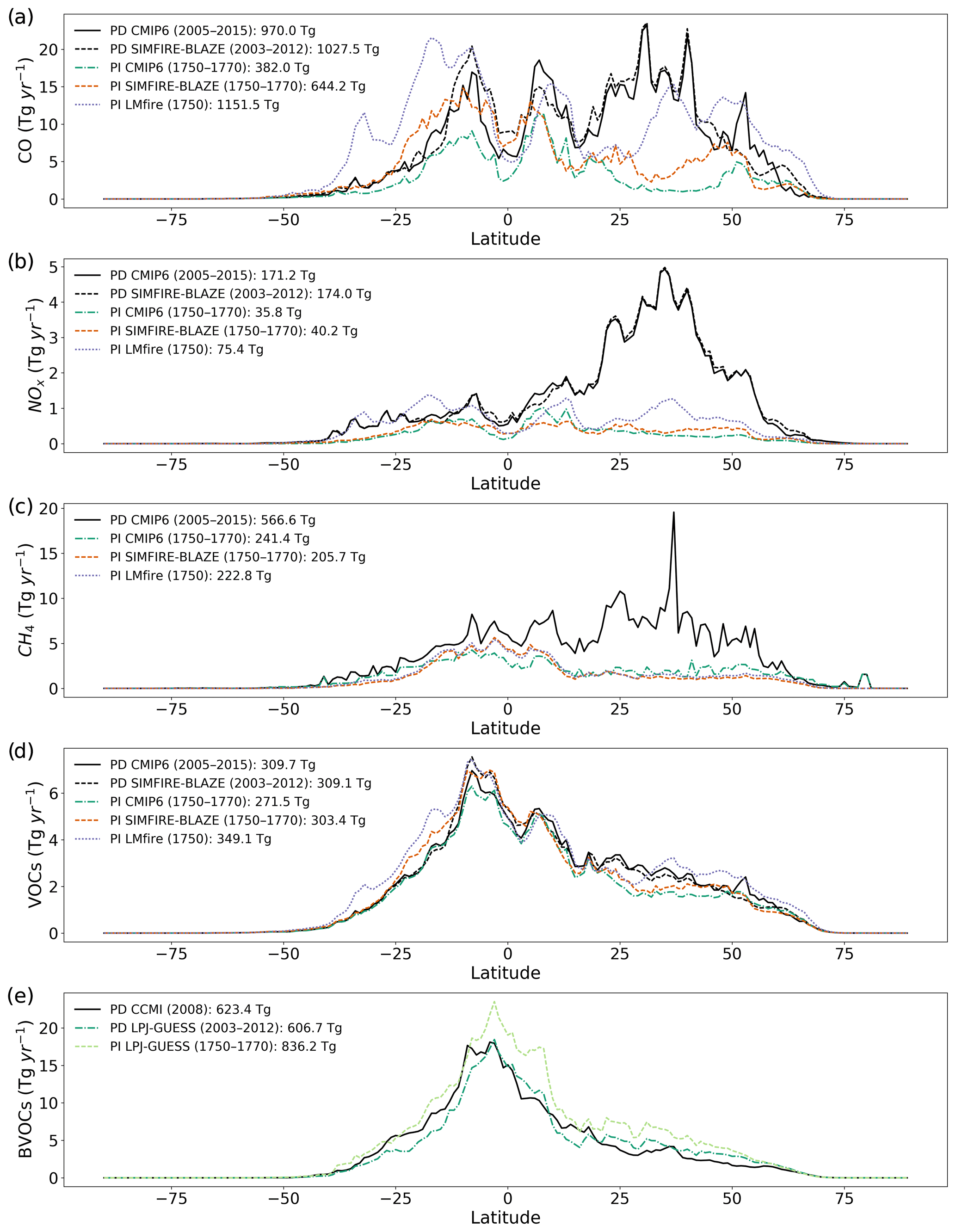
Figure 1 Annual latitudinal mean pre-industrial emissions (Tg yr⁻¹) of (a) CO, (b) NO_x, (c) CH₄ and (d) VOCs in the PD CMIP6 (solid black line), PD SIMFIRE-BLAZE (dashed black), PI CMIP6 (dashed green), PI SIMFIRE-BLAZE (dotted orange) and PI LMfire (dashed purple) inventories. (e) Annual latitudinal mean BVOC emissions (Tg yr⁻¹) in PD CCMI (solid black line), PD LPJ-GUESS (dashed dark green) and PI LPJ-GUESS (dotted light green).

2.4.3 Pre-industrial LPJ-LMfire

The LPJ-LMfire model calculates dry matter consumed by fire and simulates natural wildfire ignition from lightning (Pfeiffer et al., 2013; Murray et al., 2014). Land use is prescribed for the year 1770 using the KK10 scenario from Kaplan et al. (2011); climate forcing comes from a 1020-year detrended, interannually variable equilibrium dataset representing late 19th century conditions (see Pfeiffer et al., 2013, Sect. 3.4 for details). Akagi et al. (2011) emissions factors were again used to calculate the gas-phase fire emissions from dry biomass burned in each grid cell. Burned area is calculated based on fuel availability. LMfire includes emissions from managed agricultural burning, with 50 % of the litter on 20 % of croplands burden annually. Also included are emissions from post-harvest agricultural burning, with 10 % of harvested agricultural crop material assumed to be burned each year. Total PI fire emissions in LMfire are approximately double the SIMFIRE-BLAZE inventory and thus 4 times larger than CMIP6 emissions.

2.5 Assessment of PI fire emissions

Although the PI LMfire and PI SIMFIRE-BLAZE emissions are substantially larger than the PI CMIP6 emissions, both inventories fall with the current uncertainty range for fire emissions, deemed to differ by up to a factor of ∼4 (Lee et al., 2013; Hamilton et al., 2018; Pan et al., 2020). In Hamilton et al. (2018), both the SIMFIRE-BLAZE and LMfire PI inventories were shown to compare more favourably than CMIP6 to changes in PI-to-PD ice core BC measurements in the Swiss Alps. Furthermore, the LMfire emissions result in simulated aerosol concentrations that were closer to Northern Hemisphere (NH) ice core records in Greenland and Wyoming than both the CMIP6 and SIMFIRE-BLAZE emissions (Hamilton et al., 2018). In addition to the extensive examination of paleoenvironmental archives with PI fire emissions datasets by Hamilton et al. (2018), here we compared simulated annual mean surface PI CO concentrations in Antarctica for each fire emissions inventory using the Southern Hemisphere (SH) ice core CO record from Wang et al. (2010). Simulated Antarctic CO concentrations using PI CMIP6 emissions are 37 ppb, substantially lower than the Wang et al. (2010) 1750 value of 45±5 ppb. This CMIP6 value is closer to the 650-year minimum that occurred in the mid-17th century (38 ppb). When using SIMFIRE-BLAZE and LMfire emissions, Antarctic CO concentrations for 1750 are estimated at 48 and 61 ppb, respectively. The overestimation when using LMfire suggests that SH CO emissions may be high for 1750; however, they are comparable to the peak CO concentration measured in the late 1800s (55±5 ppb) when fire emissions also peaked (van der Werf et al., 2013). As 1850 is also sometimes used as the PI baseline year when calculating RF, we suggest that LMfire provides a realistic upper bound to possible PI fire emissions.

The combined evaluation of these inventories in Hamilton et al. (2018) and here indicates that although the revised PI fire inventories differ considerably from each other and are substantially larger than CMIP6 in some regions, they result in simulated PI atmospheric concentrations that more closely represent the changes observed in paleoenvironmental archives of changes in industrial era fire activity than CMIP6 estimates do. Therefore, their respective impacts on PI tropospheric O₃ concentrations and RF estimates need to be carefully considered.

2.6 Biogenic emission inventories

2.6.1 Present-day CCMI

The PD control biogenic emissions were provided from the CCMI inventory. CCMI mean annual BVOC emissions, comprising isoprene and monoterpenes, are derived using the Model of Emissions of Gases and Aerosols from Nature (MEGAN; Guenther et al., 2012) under the MACC project (Sindelarova et al., 2014). The CCMI inventory estimates global BVOC emissions at 623 Tg yr⁻¹, in reasonable agreement with surface flux measurements and other modelling studies (Arneth et al., 2008; Sindelarova et al., 2014; Rap et al., 2018).

2.6.2 Pre-industrial and present-day LPJ-GUESS

Alternative biogenic emissions were produced using the LPJ-GUESS dynamic vegetation model simulating isoprene and monoterpenes (Arneth et al., 2007; Schurgers et al., 2009). Total PD emissions and distribution in the LPJ-GUESS inventory (i.e. 607 Tg yr⁻¹) are similar to the PD CCMI inventory (Fig. 2). For the PI emissions, the LPJ-GUESS biogenic emissions inventory is based on the mean for the period 1750–1770, estimated to be 836 Tg yr⁻¹. There are large spatial differences between the PI LPJ-GUESS and PD CCMI inventories, with significantly higher emissions in South America and central Africa and lower emissions in South East Asia in the PI LPJ-GUESS inventory (Fig. 2).

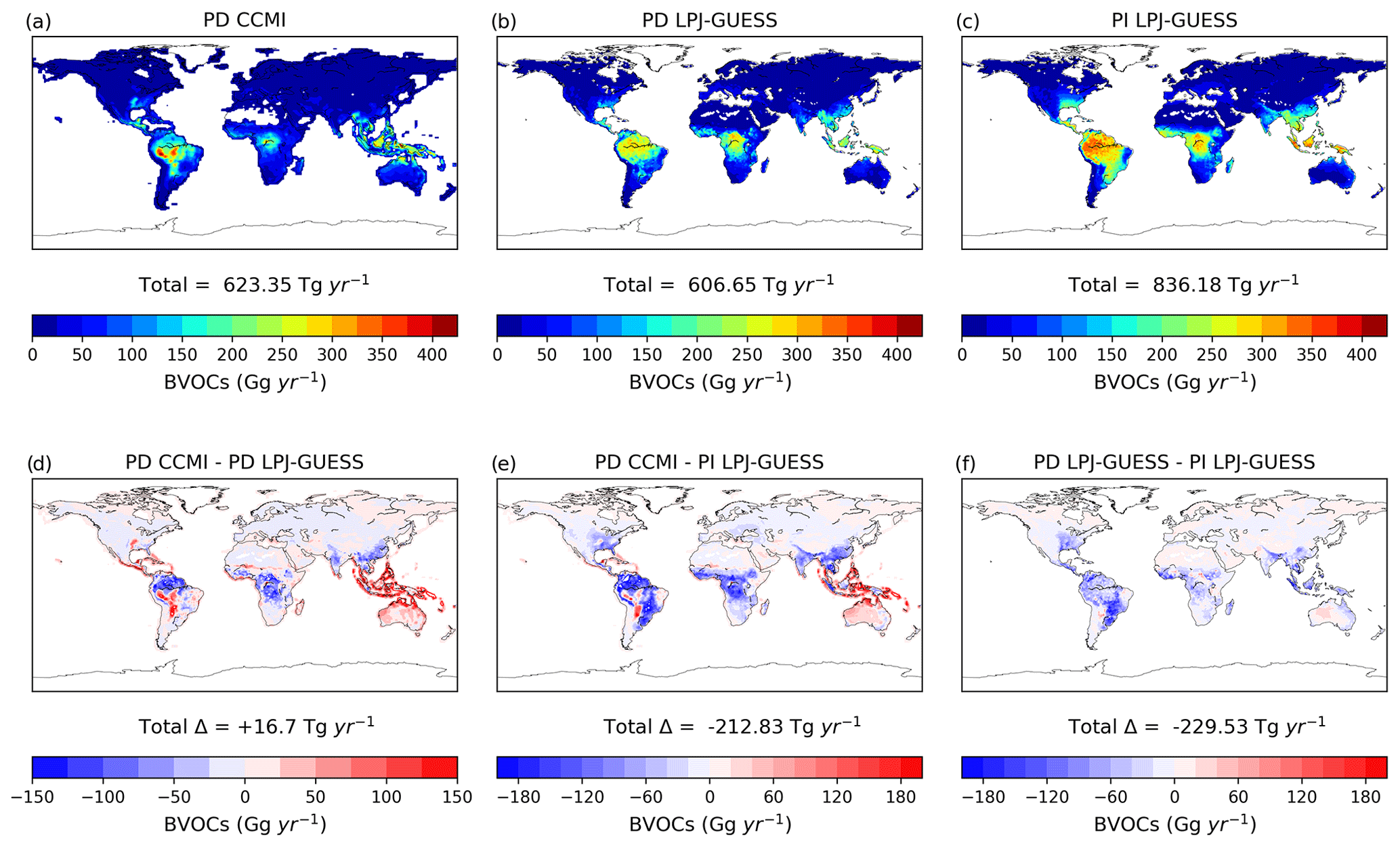
Figure 2 Annual BVOC (isoprene + monoterpenes) emissions at ${\mathrm{1}}^{\circ }\times {\mathrm{1}}^{\circ }$ resolution in the two present-day biogenic emissions inventories (CCMI and LPJ-GUESS) and the pre-industrial LPJ-GUESS inventory. (a–c) Total emissions per year and (d–f) differences between the three inventories. Total annual emissions and the difference in annual emissions are also shown.

3 Results and discussion

3.1 Pre-industrial emission inventories

Figure 1a–d show annual latitudinal fire emissions of CO, NO_x, CH₄ and VOCs from all sources for the different fire inventories considered, while Fig. 1e compares BVOC emissions (i.e. isoprene and all monoterpenes) from the biogenic inventories. There is large variation in simulated CO emissions between the three PI fire inventories: 644 Tg yr⁻¹ in SIMFIRE-BLAZE (69 % larger than CMIP6) and 1152 Tg yr⁻¹ in LMfire (200 % larger). Estimates of CO emissions using LMfire result in total global emissions which are larger than the PD estimate, which also includes anthropogenic sources. The larger PI biomass burning emissions in LMfire are a result of a number of factors not present in the other PI inventories such as the inclusion of high-latitude fire occurrence, agricultural fire emissions and differing emission factors (Hamilton et al., 2018). The largest increase occurs due to increased SH burning in the LMfire inventory, substantially increasing CO emissions from Australia and South America (particularly eastern Amazonia and Argentina). In the CMIP6 simulations, global CO emissions are increased by a factor of 2.5 between PI and PD from 382 to 970 Tg yr⁻¹. The main driver of this increase is industrial emissions, particularly in the NH mid-latitudes.

Global NO_x emissions also vary considerably between PI inventories, with values in the SIMFIRE-BLAZE inventory increasing 13 % compared to the CMIP6 inventory (36 compared to 32 Tg yr⁻¹). This difference is largely due to increased emissions in NH mid-latitudes within SIMFIRE-BLAZE. NO_x emissions in LMfire are 112 % larger than the CMIP6 total (68 Tg yr⁻¹), with the most significant increases in the extratropics.

As CH₄ emissions from fires are significantly smaller than CO emissions (Voulgarakis and Field, 2015), increased PI fire estimates do not substantially alter total CH₄ emissions. CH₄ emissions in SIMFIRE-BLAZE and LMfire are similar in amount and distribution: 15 % and 9 % lower than CMIP6, respectively. There is an increase in SH CH₄ emissions in both SIMFIRE-BLAZE and LMfire compared to CMIP6 but a decrease in the NH and SH mid-latitudes. Total PI CH₄ emissions are greatest in CMIP6 at 241 Tg yr⁻¹, approximately 43 % of PD emissions. PD SIMFIRE-BLAZE emissions of CH₄ from biomass burning were not available; therefore, PD CMIP6 CH₄ was applied in the PD SIMFIRE-BLAZE simulation. Due to the scaling of global mean surface CH₄ concentrations in TOMCAT–GLOMAP, the effect of changes in the amount of CH₄ emitted is likely small; however, the change in distribution may impact the formation and loss rates of tropospheric O₃.

In terms of fire-emitted VOC species, their magnitude and distribution of emissions are fairly consistent between PD and PI inventories. PI CMIP6 is 87 % of PD CMIP6 values, with PI SIMFIRE-BLAZE at 97 % (303 Tg yr⁻¹). Total global VOC emissions are largest in LMfire at 349 Tg yr⁻¹, 29 % larger than PI CMIP6 (271 Tg yr⁻¹) and 13 % larger than PD CMIP6 (310 Tg yr⁻¹). The distribution of total global VOC emissions is relatively uniform across all inventories; however, individual species do have larger variability between inventories. Formaldehyde and acetylene, for example, have substantially increased SH emissions in SIMFIRE-BLAZE and LMfire due to differences in emission factors, vegetation type and burned area between the fire models.

The BVOC emissions in the two PD inventories (CCMI and LPJ-GUESS) are similar (Fig. 1e), although a small positive NH gradient exists in PD LPG-GUESS compared to PD CCMI. Total BVOC emissions are 16.7 Tg larger in the PD CCMI inventory than PD LPJ-GUESS (Fig. 2). However, the PI LPJ-GUESS BVOC estimate (836 Tg yr⁻¹) is 37 % larger than its PD equivalent and 34 % larger than PD CCMI, although with a similar spatial distribution (Fig. 2). The largest difference is in South American emissions, for which PI LPJ-GUESS emissions are up to 120 Tg larger than PD. The reduction of BVOC emissions between PI and PD is due to a combination of crop expansion, land-cover changes and CO₂ inhibition (Hantson et al., 2017). Our results are consistent with previous studies reporting between ∼25 % (Lathière et al., 2010; Pacifico et al., 2012; Hollaway et al., 2017) and ∼35 % (Unger, 2014) larger PI values than PD.

The seasonality of fire emissions in the PD and PI inventories used here is demonstrated in Fig. 3. CMIP6 PI and PD emissions have an extremely similar seasonal cycle for all species, with monthly values offset by larger emissions in PD. This is expected as the PI CMIP6 emissions are based on GFED4s climatology and monthly patterns were assumed not to have changed over time (van Marle et al., 2017). The seasonal cycle of CO emissions (Fig. 3a) varies substantially across the three PI inventories, with LMfire estimating peak emissions in May–June as opposed to July–August in CMIP6 and SIMFIRE-BLAZE. This may be a result of increased emissions from SH Africa and Central America, where large fire events are common in late spring. The inclusion of high-latitude fire occurrence and agricultural burning in LMfire may also play a role, as these contribute to fire emissions in the boreal spring season (Hamilton et al., 2018). The SIMFIRE-BLAZE CO emissions exhibit a similar but more pronounced seasonal cycle than that in CMIP6, with peak emissions in August. Similarly, NO_x and VOC emissions peak earlier in the year in the LMfire inventory relative to SIMFIRE-BLAZE and CMIP6, again with a larger peak in August in SIMFIRE-BLAZE. Monthly CH₄ emissions are broadly consistent across all inventories, with peak emissions in July or August and lower emissions over the NH winter. The seasonality of BVOC emissions is also consistent across all PI inventories and PD CMIP6, with a peak in July–August. Isoprene emissions are heavily dependent on temperature and photosynthetic active radiation (Malik et al., 2018), therefore reaching a maximum in NH summer when these parameters are optimum for vegetation emissions.

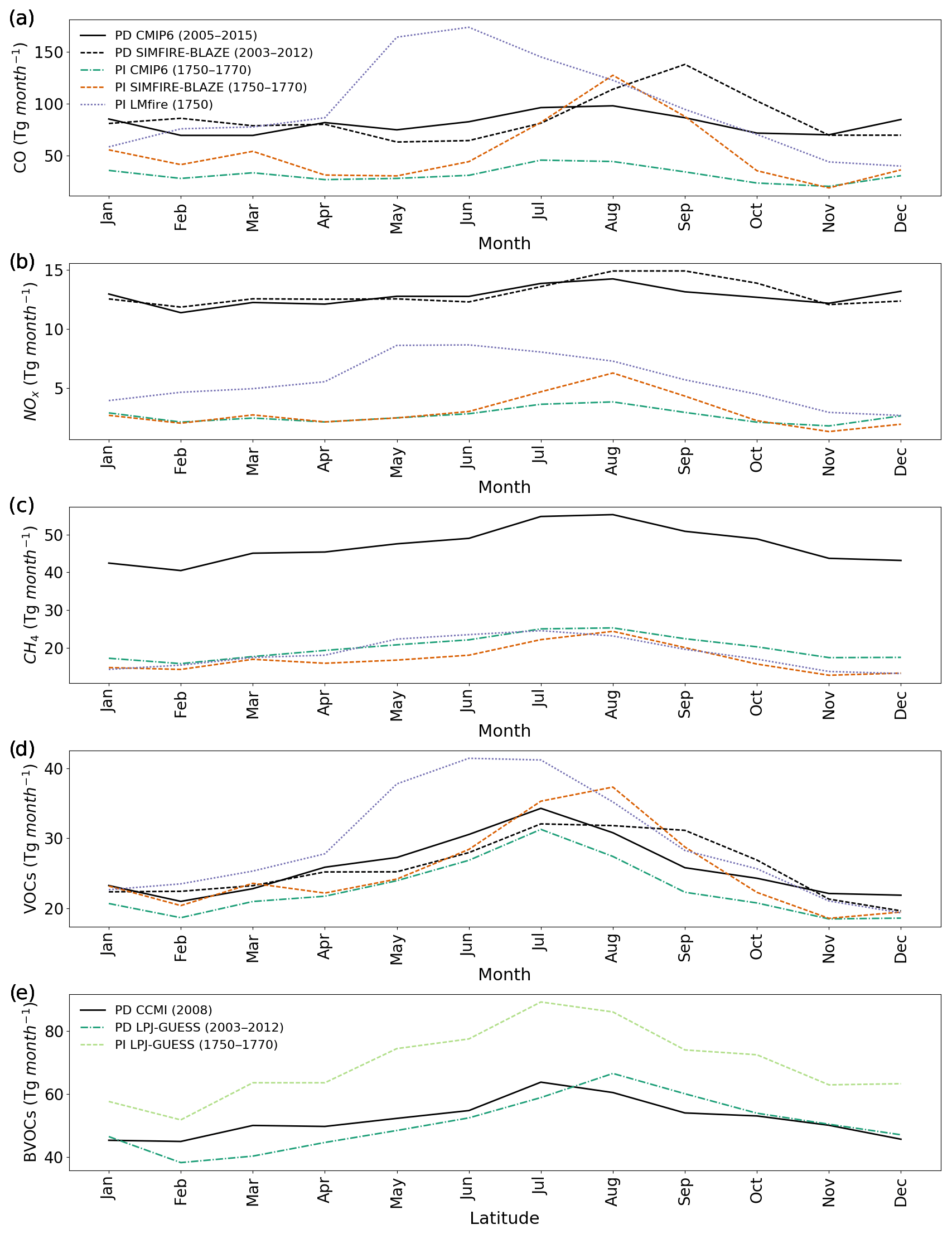
Figure 3 Total monthly emissions (Tg per month) of (a) CO, (b) NO_x, (c) CH₄, (d) VOCs and BVOCs (e) for PD CMIP6 (solid black line), PD SIMFIRE-BLAZE (dashed black), PI CMIP6 (dashed green), PI SIMFIRE-BLAZE (dotted orange), PI LMfire (dashed purple), PD LPJ-GUESS (dashed dark green) and PI LPJ-GUESS (dotted light green). The legend in panel (a) also applies to panels (b), (c) and (d).

Figure 3 indicates similar controls over the modelled seasonality of PI fire occurrence in both PI CMIP6 and PI SIMFIRE-BLAZE, with an increase in estimates of fire extent in SIMFIRE-BLAZE resulting in a more pronounced seasonal cycle. LMfire, on the other hand, estimates a shift in the seasonality of global fire emissions, with larger fire emissions earlier than other inventories, as well as a broader peak period of emissions. The change in the seasonality of precursors will undoubtedly affect the formation and transport of tropospheric O₃, as atmospheric chemistry and circulation also strong have seasonal cycles. However, the broadly similar pattern of maximum emissions in the NH summer and a minimum in winter, coinciding with similar climatic conditions, mean that the substantial difference in the volume of precursor emissions across the PI inventories is likely to be more significant than seasonal changes.

3.2 Pre-industrial fire emission effect on O₃

Annual emissions of O₃ precursors and their contribution to the formation of tropospheric O₃ are shown in Fig. 4. The largest difference between simulations is estimates of the global tropospheric CO burden, which varies by up to 100 Tg depending on the PI fire emission inventory employed: 195 Tg in the PI CMIP6 simulation, 232 Tg in PI SIMFIRE-BLAZE (18 % higher than CMIP6) and 295 Tg in PI LMfire (50 % higher) (Table 2).

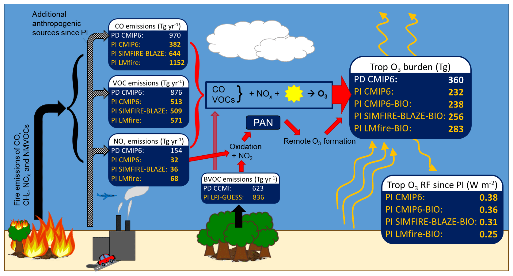
Figure 4 Summary schematic showing tropospheric O₃ precursor emissions from fire, biogenic and anthropogenic sources, the processes of photochemical O₃ formation, the tropospheric O₃ burden, and the PI-to-PD RF. The magnitude of CO, NO_x, VOC and BVOC precursor emissions used in this study is shown for the PD (white text) and each PI inventory (yellow text). The resulting calculated tropospheric O₃ burden and RF when using each emission inventory are also shown.

The difference in global NO_x burden between PI simulations is less pronounced, with increases of 4 % and 18 % in PI SIMFIRE-BLAZE and PI LMfire, respectively, relative to PI CMIP6. The annual mean NH ∕ SH ratio of tropospheric NO_x burden in PI simulations is 1.09, 1.12 and 1.18 for CMIP6, SIMFIRE-BLAZE and LMfire, respectively. The hydroxyl radical (OH), which plays a key role in regulating tropospheric O₃ concentrations, had lower PI concentrations than in PD due to the higher concentrations of the OH precursors NO_x and O₃ in PD outcompeting the effect of increased CH₄ and CO concentrations, which deplete OH (Naik et al., 2013). This is consistent in the TOMCAT PI simulations, with air-mass-weighted global mean concentrations of tropospheric OH at 1.06, 1.06 and 1.11×10⁶ molec. cm⁻³ in CMIP6, SIMFIRE-BLAZE and LMfire, respectively, compared to 1.12×10⁶ molec. cm⁻³ in PD CMIP6. Each of these values falls within 1 standard deviation of the Atmospheric Chemistry and Climate Model Intercomparison Project (ACCMIP) multi-model mean of 1.13±0.17 (Naik et al., 2013).

Changes to the atmospheric concentration and distribution of O₃ precursor species lead to changes in the tropospheric O₃ burden. The PI CMIP6 simulation produced the lowest tropospheric O₃ burden at 232 Tg, slightly below the ACCMIP multi-model mean of 239 Tg for 1850 (Young et al., 2013). In PI SIMFIRE-BLAZE the burden is 242 Tg (4 % higher than CMIP6), while in LMfire it is 273 Tg (18 % higher), slightly outside the range of estimates of 1850 tropospheric O₃ burden in ACCMIP models (192 to 272 Tg) (Young et al., 2013). The burdens simulated here represent a PI-to-PD tropospheric O₃ burden change of 55 %, 49 % and 32 % for CMIP6, SIMFIRE-BLAZE and LMfire, respectively. We note that PI LMfire is the only inventory leading to a simulated PI-to-PD global burden change of less than 40 %, a value consistent with that recently indicated by isotope measurements in ice cores (Yeung et al., 2019). The differences between CMIP6 and SIMFIRE-BLAZE are primarily related to increases in tropospheric O₃ within the Amazon region (Fig. 5a). The change in the tropospheric O₃ vertical profile in the PI SIMFIRE-BLAZE simulation compared to PI CMIP6 (Fig. 5c) shows increased annual mean concentrations throughout the troposphere, driven by changes at 30^∘ S and 50^∘ N. Changes between LMfire and CMIP6 simulated tropospheric O₃ profiles are larger, with increased O₃ at all latitudes. Compared to PI CMIP6, there is a mean global increase in the O₃ column of 3.7 DU when using LMfire and 1.0 DU when using SIMFIRE-BLAZE. The largest changes occur over central Asia, Australia and South America where tropospheric column O₃ can be as much as 9.0 DU higher in the PI LMfire simulation than the PI CMIP6 simulation (Fig. 5b). This is reflected in the changes to the vertical O₃ profile, with the largest increases in the subtropics. The difference between LMfire and CMIP6 simulations is greatest between 600 and 800 hPa in the SH and is roughly constant with respect to changes in altitude over the northern subtropics. The only regions where tropospheric O₃ is higher in the CMIP6 simulation are central Africa and Indonesia, likely due to the PI CMIP6 emissions being anchored to PD fire observations and thus transferring these patterns to the PI (van Marle et al., 2017).

Figure 5 Difference in simulated PI O₃ between the CMIP6 control and the revised inventories SIMFIRE-BLAZE and LMfire. (a, b) A comparison of differences in tropospheric column O₃ in DU; (c, d) differences in zonal mean vertical O₃ (ppbv).

The effect of different fire emission inventories on the O₃ burden is significantly smaller than the impact on CO concentrations (Table 2), as fire emissions are one of several sources of O₃ variability (Lelieveld and Dentener, 2000). O₃ production is reliant on a number of precursors which do not respond uniformly to the different estimates of fire occurrence in the inventories used here. The relatively minor response of NO_x concentrations across the three PI emission estimates (Table 2), and the prevailing NO_x-limited state across rural environments in PD (Duncan et al., 2010), suggests that increases in CO and VOCs have only a small impact on O₃ production because of NO_x availability limitations. Moreover, Stevenson et al. (2013) attributed the majority of the PI-to-PD shift in tropospheric O₃ to NO_x and CH₄ changes, with a relatively small contribution from CO and NMVOCs despite increasing emissions of both. However, the simulated changes still represent significant shifts in the abundance and distribution of tropospheric O₃ in the PI atmosphere.

3.3 Pre-industrial BVOC emission effect on O₃

We repeated the three PI simulations, replacing the PD biogenic emissions with the PI LPJ-GUESS inventory. In general, the inclusion of PI BVOC emissions increases PI O₃ concentrations due to an increased VOC source and hence PAN formation (Fig. 4). For CMIP6 fire emissions, the inclusion of PI BVOCs increases the CO burden by 22 % and the tropospheric O₃ burden by 3 %, while the mean tropospheric OH concentration decreases by 6 %. The decrease in OH is likely responsible for the simulated increase in CO, as OH is consumed by VOC oxidation. The increase in global tropospheric O₃ indicates that the simulated increases in VOC and CO concentrations are co-located with high NO_x concentrations, as in low NO_x BVOCs may decrease local O₃ concentrations. The inclusion of PI BVOCs in the LMfire fire emission simulation causes a 3 % decrease in tropospheric OH and increases in tropospheric CO and O₃ of 14 % and 4 %, respectively.

For SIMFIRE-BLAZE, the inclusion of PI BVOCs decreases OH by 6 % and increases CO and O₃ by 22 % and 6 %, respectively. In all simulations the inclusion of PI BVOCs has only a small effect on the NO_x burden (∼1 %). The effect on tropospheric O₃ of including PI BVOCs is notably larger in the simulation using SIMFIRE-BLAZE fire emissions compared to CMIP6 or LMfire. The SIMFIRE-BLAZE simulation combines fire and biogenic emissions produced using the same land-use model, with consistent vegetation distributions. The co-location of isoprene and NO_x emissions promotes PAN formation, enabling long-range transport of NO_x and enhancing O₃ production (Hollaway et al., 2017). This synergistic effect has been found to amplify the effect of biogenic emissions on tropospheric O₃ production (Bossioli et al., 2012). Therefore, if PI biogenic emissions inventories were specifically produced for each fire inventory, the corresponding impact on O₃ would likely be larger than presented here. With the inclusion of PI BVOC emissions, both the SIMFIRE-BLAZE and LMfire simulations result in a PI-to-PD tropospheric O₃ burden change of 40 % or less, in line with estimates from oxygen isotope measurements from ice cores (Yeung et al., 2019).

3.4 Effect on ozone radiative forcing

The estimated tropospheric O₃ RF, based on the CMIP6 PI and PD control simulations, is 0.38 W m⁻² (Fig. 4 and Table 2), comparing well with the IPCC AR5 estimate of 0.4±0.2 W m⁻² (Myhre et al., 2013; Stevenson et al., 2013). We obtain the same 0.38 W m⁻² RF value when contrasting the PI CMIP6 simulation against the other the other PD simulation (PD SIMFIRE-BLAZE). This is consistent with the fact that PD tropospheric O₃ is well constrained by satellite observations (Rap et al., 2015). Given the similarity of the PD simulations, the main PD CMIP6 simulation is used here as the PD for RF calculations in this section. When PI SIMFIRE-BLAZE and PI LMfire emissions are used instead of PI CMIP6 fire emissions, larger PI tropospheric O₃ concentrations lead to 8 % (to 0.35 W m⁻²) and 29 % (to 0.27 W m⁻²) decreases in O₃ RF, respectively. When the PI BVOC emission inventory is used in conjunction with each PI fire emission inventory, O₃ RF is further reduced compared to the control by 5 % (to 0.36 W m⁻²), 18 % (to 0.31 W m⁻²) and 34 % (to 0.25 W m⁻²) for CMIP6, SIMFIRE-BLAZE and LMfire, respectively (Fig. 4). While these reductions in O₃ RF are still within the IPCC uncertainty range, they are caused entirely by uncertainty in PI precursor emissions from wildfires and vegetation. Other key sources of uncertainty (e.g. inter-model spread, use of different radiative transfer schemes) are not accounted for here and would therefore alter estimates further, potentially outside the current 5 %–95 % confidence range. The most important region for changes to the RF of O₃ is the upper troposphere at subtropical latitudes (Fig. 5d), where there are substantially higher O₃ concentrations in the LMfire simulation. O₃ changes in this region are up to 10 times more efficient at altering the radiative flux than in other regions (Rap et al., 2015). However, the lack of a vertical distribution to fire emissions in TOMCAT affects the simulated changes to the O₃ vertical profile. Previous studies, which introduced an injection height scheme, found small increases in O₃ production downwind of emission sources (Jian and Fu, 2014), although the change to total O₃ and precursors is relatively small (Bossioli et al., 2012; Zhu et al., 2018).

4 Conclusions

Revised inventories of PI fire and biogenic emissions substantially decrease estimates of PI-to-PD tropospheric O₃ RF. When using PI LMfire fire emissions, which represent a plausible upper emissions limit, O₃ RF is reduced to 0.27 W m⁻², 29 % smaller than the CMIP6 simulation. Large increases in estimated PI fire occurrence drive increases in PI O₃ concentrations (3.7 DU global mean tropospheric column O₃ increase for LMfire inventory) through larger emissions of CO, NO_x and VOCs. PI CO increases by up to 51 % depending on the PI inventory, but the effect on O₃ production is limited by the relatively small increase in NO_x (∼4 %). Using PI biogenic emissions, rather than assuming PD values, further increases simulated PI tropospheric O₃, though the magnitude of this depends on the fire inventory. When accounting for revised emissions from fire and biogenic sources, both the LMfire and SIMFIRE-BLAZE inventories simulated a PI-to-PD change in the tropospheric O₃ burden of approximately 40 % or less, in good agreement with estimates from Yeung et al. (2019). Consequently, we find that the estimate of O₃ RF since PI decreases by up to 34 % (to 0.25 W m⁻²) when considering the uncertainty in PI emissions of both fires and BVOCs.

The impact on tropospheric O₃ from uncertainty in PI natural emissions suggests that previous estimates of O₃ RF over the industrial era are likely too large. Our revised tropospheric O₃ RF estimates are at the lower end of the existing uncertainty range, without yet taking into account other sources of uncertainty. We therefore argue that the impact of uncertainty on PI natural emissions should be further investigated using more models in order to reassess the current best estimate and uncertainty range of O₃ RF.