Attribution of ground-level ozone to anthropogenic and natural sources of nitrogen oxides and reactive carbon in a global chemical transport model

We perform a source attribution for tropospheric and ground-level ozone using a novel technique that accounts separately for the contributions of the two chemically distinct emitted precursors (reactive carbon and oxides of nitrogen) to the chemical production of ozone in the troposphere. By tagging anthropogenic emissions of these precursors according to the geographical region from which they are emitted, we determine source–receptor relationships for ground-level ozone. Our methodology reproduces earlier results obtained via other techniques for ozone source attribution, and it also delivers additional information about the modelled processes responsible for the intercontinental transport of ozone, which is especially strong during the spring months. The current generation of chemical transport models used to support international negotiations aimed at reducing the intercontinental transport of ozone shows especially strong inter-model differences in simulated springtime ozone. Current models also simulate a large range of different responses of surface ozone to methane, which is one of the major precursors of ground-level ozone. Using our novel source attribution technique, we show that emissions of NO_x (oxides of nitrogen) from international shipping over the high seas play a disproportionately strong role in our model system regarding the hemispheric-scale response of surface ozone to changes in methane, as well as to the springtime maximum in intercontinental transport of ozone and its precursors. We recommend a renewed focus on the improvement of the representation of the chemistry of ship NO_x emissions in current-generation models. We demonstrate the utility of ozone source attribution as a powerful model diagnostic tool and recommend that similar source attribution techniques become a standard part of future model intercomparison studies.

1 Introduction

Tropospheric ozone plays a central role in the chemistry and self-cleansing capacity of the troposphere (Crutzen, 1973; Monks et al., 2015); however, at high concentrations close to the ground, it is harmful to human health (Haagen-Smit, 1952; Fleming et al., 2018) and vegetation (Reich and Amundson, 1985; Mills et al., 2018). As well as being transported into the troposphere through exchange with the stratosphere, ozone can be formed via chemical reactions in the troposphere involving two chemically distinct precursors: oxides of nitrogen (collectively NO_x) and reactive carbon species, including carbon monoxide, methane, and volatile organic compounds (Crutzen, 1973; Atkinson, 2000). Increases in tropospheric ozone since preindustrial times have been attributed primarily to increases in anthropogenic emissions of NO_x and methane – the latter of which is the most abundant reactive carbon species in the atmosphere (Wang and Jacob, 1998; Stevenson et al., 2013).

Ozone is long-lived enough in the troposphere to circumnavigate the Northern Hemisphere along the prevailing westerly winds (Jacob et al., 1999). Thus, emissions of NO_x or reactive carbon in any Northern Hemisphere source region can contribute to the ozone mixing ratio in any other region of the Northern Hemisphere. This long-range contribution to the ozone mixing ratio is often referred to as “baseline” ozone (Parrish et al., 2017; Derwent et al., 2018). Due to seasonal variation in the lifetime of ozone, this effect is strongest in spring and weakest in summer (Fiore et al., 2009). The ambient ozone mixing ratio at any location is a combination of ozone transported from the hemispheric background and in-situ photochemical production. Recent analyses of long-term trends in baseline ozone in western regions of North America (Parrish et al., 2017) and Europe (Derwent et al., 2018) have shown increasing trends since reliable measurements began in the 1980s until approximately 2000–2010, and they indicate that these trends may be beginning to reverse.

Figure 1 Seasonal cycle of monthly mean surface ozone (ppb) in Hemispheric Transport of Air Pollution (HTAP) Tier 2 regions from our base model run (blue line), compared with observations from the Tropospheric Ozone Assessment Report (TOAR; black line), and other models from the HTAP ensemble of global models: ensemble mean (red line), ensemble standard deviation (green shaded area), and ensemble range (grey shaded area). Only grid cells containing TOAR observations have been used.

Chemical transport models (CTMs) are commonly used to interpret observations of ozone and to synthesize an understanding of the fundamental processes controlling its origin and fate in the atmosphere in order to project future trends (e.g. Young et al., 2018). The range in values of the surface ozone mixing ratio over the Northern Hemisphere simulated by contemporary CTMs is extremely high (see, for example, our Fig. 1 in Sect. 3), requiring the use of a large ensemble of models (e.g. HTAP, 2010; Young et al., 2018). When compared with available measurements of ozone for the Northern Hemisphere (e.g. Schultz et al., 2017), ensembles of global CTMs are generally able to simulate the spatial distribution and seasonal cycles of surface ozone; however, they are consistently biased high in the Northern Hemisphere and have difficulty simulating long-term trends (Young et al., 2018). Potential sources of uncertainty in CTMs include uncertainties in their chemical mechanisms (the representations of the relevant chemical reactions and their rates); their representation of atmospheric transport processes; and their representation of exchange processes between the atmosphere and the surface of the Earth, including emissions of the ozone precursors NO_x and reactive carbon.

The most important class of reactions for the formation of ozone in the troposphere is the reaction of NO (nitric oxide) with a peroxy radical, which is itself formed during the oxidation of reactive carbon (Atkinson, 2000). During this process, the NO is converted to NO₂ (nitrogen dioxide), which can be rapidly photolysed, ultimately forming ozone and recycling NO. The ozone production efficiency of NO_x (the combined concentration of NO and NO₂) can vary significantly depending on the location and timing of the NO_x emissions. In the polluted boundary layer, NO_x is rapidly removed from the atmosphere through the reaction of NO₂ with OH, forming HNO₃, which is subsequently lost via dry or wet deposition. Under less polluted conditions, NO₂ photolysis competes more effectively with HNO₃ production, allowing each unit of NO_x to react with a higher number of peroxy radicals before eventually being scavenged by OH, thereby leading to a higher ozone production efficiency per unit of NO_x. When NO_x is lofted into the free troposphere, its ozone productivity increases substantially (Jacob et al., 1996). Thus, emissions of NO_x in the tropics are especially effective at producing tropospheric ozone due the fact that they are transported aloft by deep convection (Zhang et al., 2016). NO_x emissions from both aircraft and lightning are also highly efficient at producing tropospheric ozone (Beck et al., 1992; Dahlmann et al., 2011). Combustion of fossil fuels is the largest source of NO_x in the atmosphere (Galloway et al., 2008).

Lawrence and Crutzen (1999) first pointed out that international shipping can have a disproportionately high influence on tropospheric ozone due to the disperse nature of NO_x emissions from this source. Hoor et al. (2009) quantified the sensitivity of tropospheric ozone to NO_x emissions from different modes of transport (land, sea, and air), finding that aircraft emissions were most efficient at producing ozone (per molecule of NO_x emitted), followed by ships and then land transport. For near-surface ozone, however, NO_x emissions from ships were shown to have a higher influence than NO_x emissions from aircraft. Nevertheless, ozone production from ship NO_x is highly uncertain in current CTMs. Kasibhatla et al. (2000) and von Glasow et al. (2003) showed that global CTMs, due to their coarse resolution (usually in the hundreds of kilometres), do not resolve the chemistry of ship exhaust plumes; instead, there is a tendency for NO_x to be removed from the atmosphere more quickly than simulated by the global CTMs, which effectively instantly dilute these emissions into very large volumes. Wild and Prather (2006) also showed that this effect applies more generally to other concentrated emission sources such as urban areas. Vinken et al. (2011) introduced a method for parameterizing ship exhaust plume chemistry using lookup tables in their global CTM, but this method has not been widely adopted by the modelling community. Modelling of ship NO_x and the effects of NO_x on the atmosphere remains a challenge for global CTMs.

The term “reactive carbon” encompasses a very wide range of atmospheric constituents (e.g. Chameides et al., 1992; Goldstein and Galbally, 2007; Heald and Kroll, 2020). In contrast to NO_x, most of the reactive carbon emitted to the atmosphere is not of anthropogenic origin but rather emitted from the biosphere. In this study, we restrict our definition to molecules that yield peroxy radicals (either hydroperoxy radicals HO₂ or organic peroxy radicals RO₂) during their gas-phase oxidation and, thus, contribute to ozone formation by potentially converting NO to NO₂. Therefore, this definition includes carbon monoxide (CO) and the large family of molecules known as volatile organic compounds (VOCs). The simplest VOC is methane, which is often considered separately from non-methane volatile organic compounds (NMVOCs) due to its very long lifetime in the troposphere. The ozone production potential of reactive carbon depends on the rate at which it is oxidized in the atmosphere, usually through reaction with the OH radical (Carter, 1994), as well as the subsequent chemistry of its oxidation products (Butler et al., 2011; Derwent, 2020). Most reactive carbon species have relatively short lifetimes in the troposphere due to their reaction with OH radicals. Methane, due to its exceptionally low reactivity, is well mixed in the troposphere. In contrast to other forms of reactive carbon, emissions of methane can contribute to ozone formation at any location in the troposphere where photochemical conditions are favourable (Fiore et al., 2008). Despite its low reactivity in comparison to other types of reactive carbon, methane is highly abundant and has been shown to make a large contribution to tropospheric ozone (Wang and Jacob, 1998; Fiore et al., 2008; Stevenson et al., 2013; Butler et al., 2018).

PAN (peroxyacetyl nitrate) is an important reservoir species for both peroxy radicals and for NO_x (Fischer et al., 2014). Peroxyacetyl radicals are formed during the oxidation of a wide range of different types of NMVOCs from a wide range of different sources. PAN is formed through the reaction of peroxyacetyl radicals with NO₂, primarily in the polluted boundary layer where both are abundant (Atkinson, 2000). The lifetime of PAN is strongly temperature dependent. At colder temperatures higher in the troposphere, PAN can be transported over long distances, and it can act as a source of NO₂ and peroxyacetyl radicals in remote regions upon subsidence and thermal decomposition (Fischer et al., 2014). The chemical mechanisms and reaction rate constants involved in the formation and decomposition of PAN vary widely between CTMs (Emmerson and Evans, 2009; Knote et al., 2015), leading to large inter-model differences in simulated PAN (Emmons et al., 2015). Fiore et al. (2018) suggested that measurements of PAN at northern midlatitude mountaintop sites in spring could provide a useful constraint on CTMs, although the number of observations available is limited.

With careful interpretation, the results of ensembles of CTMs can be used to diagnose long-range transboundary transport of ozone and to develop intercontinental source–receptor relationships, which relate the effects of precursor emissions from different regions of the Northern Hemisphere to mixing ratios of ground-level ozone in other regions of the Northern Hemisphere. An example of this is the activity of the Task Force on Hemispheric Transport of Air Pollution (TF-HTAP; HTAP, 2010), which reports to the Convention on Long-Range Transboundary Air Pollution (CLRTAP) and, thus, informs international policymaking for the mitigation of air pollution. The TF-HTAP studies used a “perturbation” approach that compared a control simulation with sensitivity simulations in which emissions of particular ozone precursors were reduced by 20 %. Combined 20 % reductions of global average methane and remote anthropogenic emissions of NO_x, CO, and NMVOCs were shown to have an approximately equal effect on annual average ozone as a 20 % reduction of local precursor emissions, indicating the strong role of long-range transport in influencing surface ozone in the Northern Hemisphere. Results derived from Phase 1 of the TF-HTAP exercise (and the Phase 2 exercise described by Galmarini et al., 2017) are discussed in more detail by Fiore et al. (2009), Reidmiller et al. (2009) and Huang et al. (2017); Jonson et al. (2018).

An alternative approach to the perturbation technique for source attribution is “tagging” (e.g. Wang et al., 1998; Dunker et al., 2002; Grewe et al., 2010, 2017; Emmons et al., 2012; Derwent et al., 2015; Butler et al., 2018; Bates and Jacob, 2020). When applied to ozone source attribution in a CTM, this technique involves labelling (or “tagging”) modelled ozone with the identity of either the geographical region in which it is chemically produced or with the identity of the emitted precursor(s) that ultimately led to its production. A common challenge faced by all tagging approaches is that the production of one molecule of ozone in the troposphere requires two precursors: one molecule of NO and one peroxy radical (produced during reactive carbon oxidation). This then poses the question of whether the ozone molecule should inherit its tag from the emitted NO_x, from the emitted reactive carbon, or in some other way? Butler et al. (2018) provides a detailed review of the different approaches to answering this question, including the trade-offs made in each case. Butler et al. (2018) also describe a novel and unique tagging methodology that allows for the separate attribution of tropospheric ozone to both its NO_x and its reactive carbon precursor, at the cost of extra computational expense compared with other tagging methodologies. Recent work from Bates and Jacob (2020) takes the approach of defining an extended odd oxygen family including peroxy radicals, which effectively shifts the production of odd oxygen purely to photolysis reactions. Further comparison of different tagging approaches is beyond the scope of this paper, but it remains an interesting topic for future work.

Tagging and perturbation are complementary approaches (Clappier et al., 2017; Thunis et al., 2019; Mertens et al., 2020). While tagging delivers information about the contribution of different emission sources to a pollutant of interest, perturbation studies deliver information about the sensitivity of pollutants to changes in emissions, including changes in the chemical lifetimes of pollutants in response to variations in emissions. In the absence of non-linear chemical interactions, these two different approaches ultimately yield the same results; however, for tropospheric ozone, which can show highly non-linear interactions between its NO_x and reactive carbon precursors under some circumstances, these approaches can sometimes yield very different results (Grewe et al., 2010; Mertens et al., 2018). As air pollution mitigation strategies must involve some change in emissions, perturbation studies will always be necessary for policy-relevant modelling of atmospheric chemistry. However, tagging studies on their own can play a role in helping to identify which emissions to mitigate (Grewe et al., 2010). When combined with perturbation studies, tagging can reveal how the contribution of unmitigated sources to ozone changes in response to mitigation measures (Mertens et al., 2018). Butler et al. (2018) also noted that tagging studies provide useful diagnostic information about model processes and argued for their inclusion in model intercomparison exercises. The method described by Butler et al. (2018) is currently the only available approach that provides the separate attribution of tropospheric ozone to its NO_x and reactive carbon precursors. Other schemes take different approaches to the attribution of ozone to these two chemically distinct precursors. A thorough review of several different approaches is presented in Butler et al. (2018).

In this study, we use the ozone tagging methodology previously described by Butler et al. (2018) to perform a source attribution for ground-level ozone to both NO_x and reactive carbon. This work builds on the work of Butler et al. (2018) by tagging anthropogenic emissions of NO_x and reactive carbon by their geographical source region as well as examining the seasonal cycle of the surface ozone attribution in receptor regions as defined in the HTAP Phase 2 exercise. By performing the separate attribution of ground-level ozone to both NO_x and reactive carbon (including methane), we hope to provide more useful information to inform emission mitigation scenarios. We also show how our tagging methodology can be used as a model diagnostic tool to understand the atmospheric budgets of ozone and PAN in more detail than previously possible, potentially informing efforts to reduce the currently high level of inter-model uncertainty. Furthermore, we examine the changing contributions of the different sources of NO_x and reactive carbon to a perturbation of the global methane burden, showing how the contribution of emissions from unmitigated sectors would respond to the mitigation of methane emissions.

The tagging approach and model set-up is described in Sect. 2. In Sect. 3, we evaluate our simulations against observations from the Tropospheric Ozone Assessment Report (TOAR) and the ensemble of simulations from HTAP Phase 2, show the intercontinental source attribution for ozone and its precursors, and examine the response of this source attribution to a 20 % perturbation in the global methane burden. Conclusions are drawn in Sect. 4.

2 Experimental design

Simulations are performed with CAM4-chem (Community Atmosphere Model version 4 with chemistry), which is a component of the CESM (Community Earth System Model) version 1.2.2 (Tilmes et al., 2015; Lamarque et al., 2012), using the same model configuration as Butler et al. (2018). The model is run at a horizontal resolution of 1.9^∘ × 2.5^∘, with 56 vertical levels using specified dynamics for the year 2010 from the MERRA reanalysis (Rienecker et al., 2011). As in Butler et al. (2018), we have replaced the default chemical mechanism with a tagged mechanism based on an earlier version of the MOZART-4 mechanism (Emmons et al., 2012). Our tagging system allows for the attribution of tropospheric ozone to chemical production by either NO_x or reactive carbon precursors (as well as transport from the stratosphere). A complete attribution of tropospheric ozone to both kinds of precursors requires two model runs: one with NO_x emissions tagged and another with reactive carbon emissions tagged. Chemical production of ozone in the stratosphere (primarily through the photolysis of molecular oxygen) and other minor production pathways for tropospheric ozone are also tagged, as described in Butler et al. (2018). For both NO_x tagging and VOC tagging, the sum of the tagged ozone tracers is equal to the total ozone as simulated by the model.

As in Butler et al. (2018), anthropogenic emissions of NO_x, CO, and NMVOCs for 2010 are taken from the EDGAR-HTAPv2 emission inventory (Janssens-Maenhout et al., 2015), biomass burning emissions are from GFEDv3 (van der Werf et al., 2010), and methane is held fixed at the surface to a global average value of 1760 ppb, as in Tilmes et al. (2015). Two simulations (base runs) are performed with this model set-up: one in which all sources of NO_x are tagged as described below (the “NO_x-tagged” run) and one in which all sources of reactive carbon are tagged as described below (the “VOC-tagged” run). As in Butler et al. (2018), the length of the spin-up period was 1 year for the NO_x-tagged run, and it was 2 years for the VOC-tagged run. The model was deemed to be spun up when the maximum difference between the simulated December mean surface ozone attributable to any tagged source was less than 1 % in any 2 subsequent years of simulation.

With the exception of surface-based anthropogenic emissions of NO_x, CO, and NMVOCs, the tag identities used in this study are identical to those used in Butler et al. (2018). In this study, all surface-based anthropogenic emissions are tagged with a label representing the geographical location at which the emissions occur. This approach allows for the attribution of simulated ozone to anthropogenic precursor emissions from specific locations. Specifically, anthropogenic emissions of NO_x and reactive carbon are tagged according to their Tier 1 source region as defined for the HTAP Phase 2 multi-model ensemble experiment, which is described in more detail in (Galmarini et al., 2017). Due to computational constraints, not all of the HTAP Tier 1 regions are tagged in this study. As the primary focus of this study is on the attribution of ground-level ozone in the Northern Hemisphere, only the major anthropogenic Northern Hemisphere source regions are tagged, whereas other anthropogenic sources are tagged with the label “Rest of the world”. A full list of the tags used in the NO_x- and VOC-tagged runs is given in Table 1. The explicitly tagged source regions differ between the NO_x-tagged and VOC-tagged runs because VOC tagging is computationally more expensive than the NO_x tagging (Butler et al., 2018). One important difference between this study and Butler et al. (2018) is that anthropogenic emissions of CO for each source region are tagged together with emissions of NMVOCs in this study in order to save computational resources. For the emissions tagged as “Oceanic emissions” (Table 1), we note that the only source of NO_x from this region in our simulations is from shipping and that the major source of reactive carbon is biogenic emissions of dimethyl sulfide (DMS).

Table 1 List of tags used for the attribution of tropospheric ozone in the NO_x- and VOC-tagged runs. Anthropogenic emissions of NO_x and reactive carbon are tagged based on their HTAP Tier 1 region. Other tags are as in Butler et al. (2018). RoW refers to “Rest of the world”.

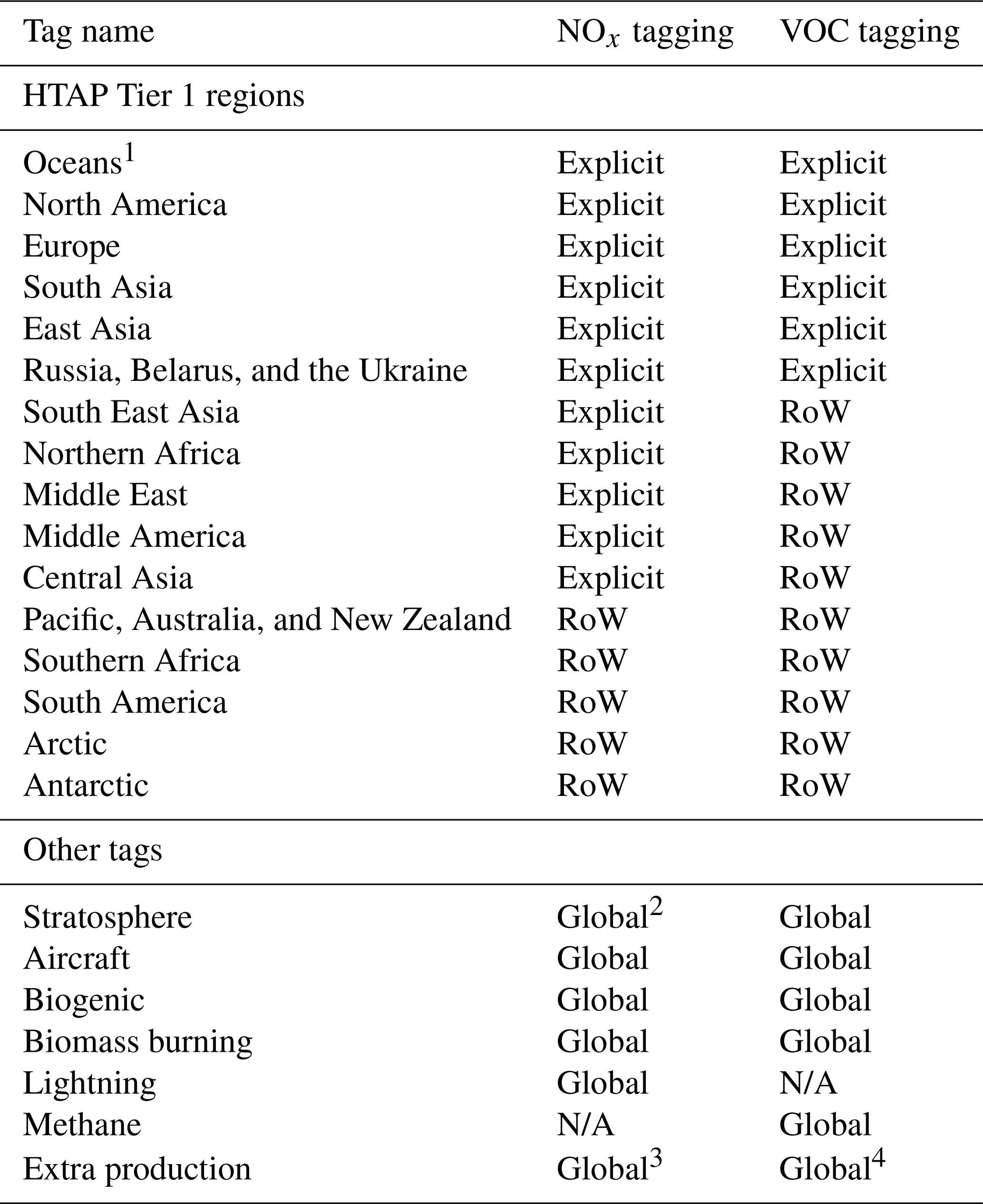
¹ NO_x from “Oceans” is exclusively from shipping, whereas reactive carbon from this region is predominantly biogenic. ² For NO_x tagging, the stratosphere tag is applied directly to ozone produced in the stratosphere (as for VOC tagging) and also to NO produced from the dissociation of N₂O. ³ For NO_x tagging, “Extra production” of ozone is due to the self reaction of OH radicals and reactions between HO₂ and organic peroxy radicals. ⁴ For VOC tagging, “Extra production” of ozone is due to the self reaction of OH radicals and reaction of OH with H₂O₂.

In addition to the NO_x- and VOC-tagged base runs described above, we also perform two additional runs in order to investigate the response of tropospheric ozone to a perturbation in the tropospheric burden of methane: one with NO_x tagging and another with VOC tagging. In each of these methane perturbation runs, the initial atmospheric methane burden and the methane mixing ratio imposed at the surface as a boundary condition are reduced by 20 %. This translates to a surface methane mixing ratio of 1410 ppb in these methane perturbation runs. In the above-mentioned perturbation runs, all other sources of NO_x and reactive carbon are left unchanged. The methane perturbation runs also require 2 years of spin-up for the model to arrive at steady state.

CAM4-chem in version 1.2.2 of the CESM has previously been evaluated by Tilmes et al. (2015), and the modified version used in this study has also been discussed thoroughly by Butler et al. (2018). In Sect. 3, we describe the key differences in methane and tropospheric ozone between our base simulation and the CAM4-chem simulation reported by Tilmes et al. (2015), and we compare our simulated surface ozone with observations from TOAR (Schultz et al., 2017) as well as with the ensemble of CTM simulations from the HTAP Phase 2 multi-model study (Galmarini et al., 2017). The full set of CTMs that participated in the HTAP Phase 2 multi-model ensemble is given in Table 3 of Galmarini et al. (2017). In this study we compare surface ozone from our base simulation with results from a subset of 12 CTMs: CAM-chem (simulations performed by the National Center for Atmospheric Research, NCAR), CHASER_re1, CHASER_t106, C-IFS, C-IFS_v2, EMEP_rv4.5, EMEP_rv48, GEM-MACH, GEOS-Chem Adjoint, GEOS-Chem, OsloCTM3.v2, and RAQMS. Details of the configurations used by each of these models in the HTAP Phase 2 ensemble can be found in Galmarini et al. (2017) and references therein.

3 Results and discussion

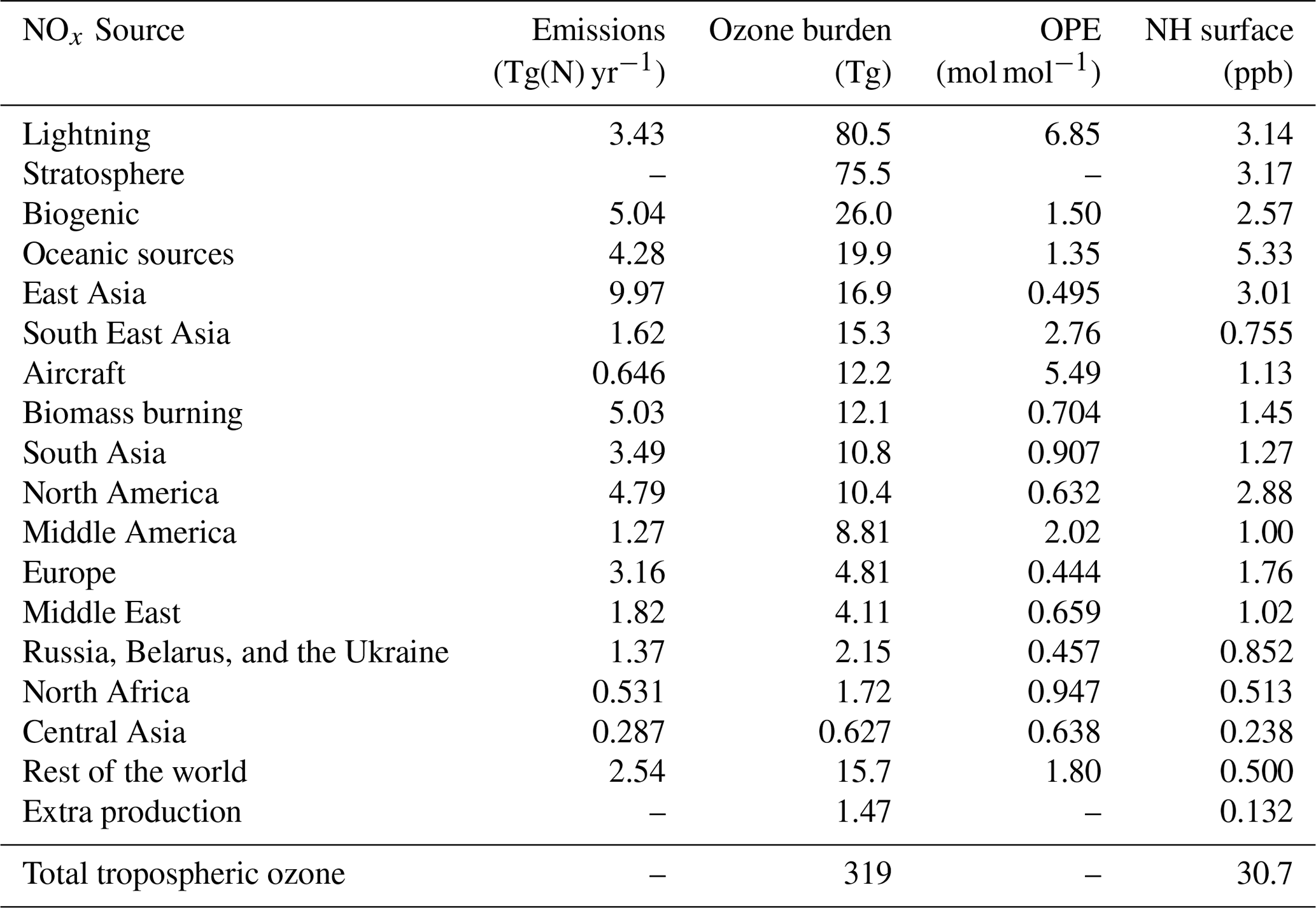
All results presented in this study are based on the definition of the troposphere as the model grid cells below the level of 150 ppb of ozone. By design, the ozone simulated in our base model runs is identical to the simulation reported in Butler et al. (2018). Our simulation for 2010 produces a tropospheric ozone burden of 319 Tg(O₃), which is within 1 standard deviation of the multi-model mean reported by Young et al. (2013) for the year 2000 (337±23 Tg(O₃)). Our simulated tropospheric ozone burden is slightly higher than the burden reported by Tilmes et al. (2015) using a similar model set-up (309 Tg(O₃)), which could be due to the use of different emissions datasets. Our simulated tropospheric methane burden (4150 Tg(CH₄)) is the same as that reported by Tilmes et al. (2015), but our methane lifetime (due to oxidation in the troposphere by OH), at 7.59 years, is shorter than the 8.82 years reported by Tilmes et al. (2015), which is also likely due to the use of different emission datasets. Our methane lifetime is towards the lower end of the range (7.1–10.6 years) simulated in CTMs, as reported by Saunois et al. (2016).

In Fig. 1, we compare our simulated monthly mean surface ozone mixing ratio for 2010 with data from TOAR and with the other models in the HTAP Phase 2 CTM ensemble. Results are shown averaged over HTAP Tier 2 receptor regions, and they only include grid cells for which TOAR observations are available. In general, most of the HTAP models overestimate the monthly mean surface ozone mixing ratio in regions where observations are available, which is consistent with the high model bias reported by Young et al. (2018). Also apparent from Fig. 1 is the large range in simulated surface ozone between members of the HTAP model ensemble, which is especially high in the northern spring, approaching a spread of approximately 30 ppb between the lowest and highest ensemble members, which is of a similar order to the Northern Hemisphere annual mean surface ozone itself. Our modelled monthly average surface ozone mixing ratio in the HTAP Tier 2 receptor regions is generally close to the HTAP ensemble mean and is usually within 1 standard deviation of the ensemble mean.

3.1 Source attribution of tropospheric ozone

The attribution of annual average tropospheric ozone to emissions of NO_x and reactive carbon precursors based on the source tags from Table 1 is shown in Figs. 2 and 3 and is quantified in Tables 2 and 3. Figures showing the attribution of monthly mean ozone are available in the Supplement. For each tagged source, Tables 2 and 3 include the respective emissions of NO_x and reactive carbon and, where applicable, the contribution of each source to the 2010 average tropospheric ozone burden, the contribution to the Northern Hemisphere 2010 annual average surface mixing ratio, and the ozone production efficiency of each emission source (defined here as the contribution of each emission source to the tropospheric ozone burden, in units of moles of ozone per mole of N or C emitted). Figures 2 and 3 show the spatial distribution of the annual average surface ozone as attributed to each source of NO_x and reactive carbon, respectively. In Fig. 2, ozone attributable to anthropogenic NO_x emissions in some source regions (specifically South East Asia, northern Africa, the Middle East, Middle America, and Central Asia) has been added to the “Rest of the world” total in order to unify the definition of this source region with the definition of this region in the VOC-tagged run. The difference in the stratospheric contribution between the NO_x- and VOC-tagged runs is due to the role of NO_x produced in the stratosphere from the dissociation of N₂O. Ozone produced in reactions involving this stratospheric source of NO_x are counted in our source attribution as stratospheric ozone, as described in Butler et al. (2018).

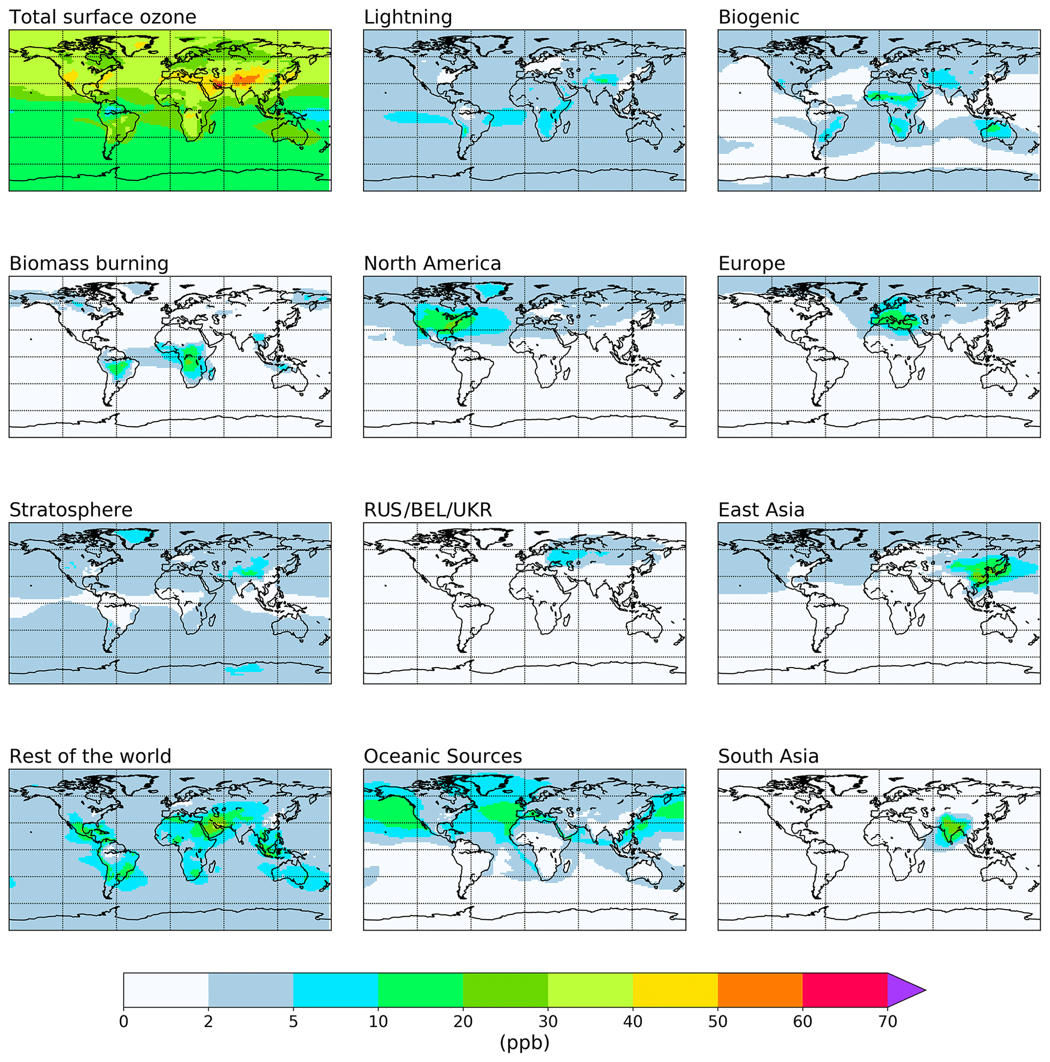
Figure 2 Annual mean surface ozone (ppb) from the NO_x-tagged base run. Total ozone is shown in the top left panel. Tagged ozone tracers are shown in the other panels. “RUS/BEL/UKR” refers to Russia, Belarus, and the Ukraine.

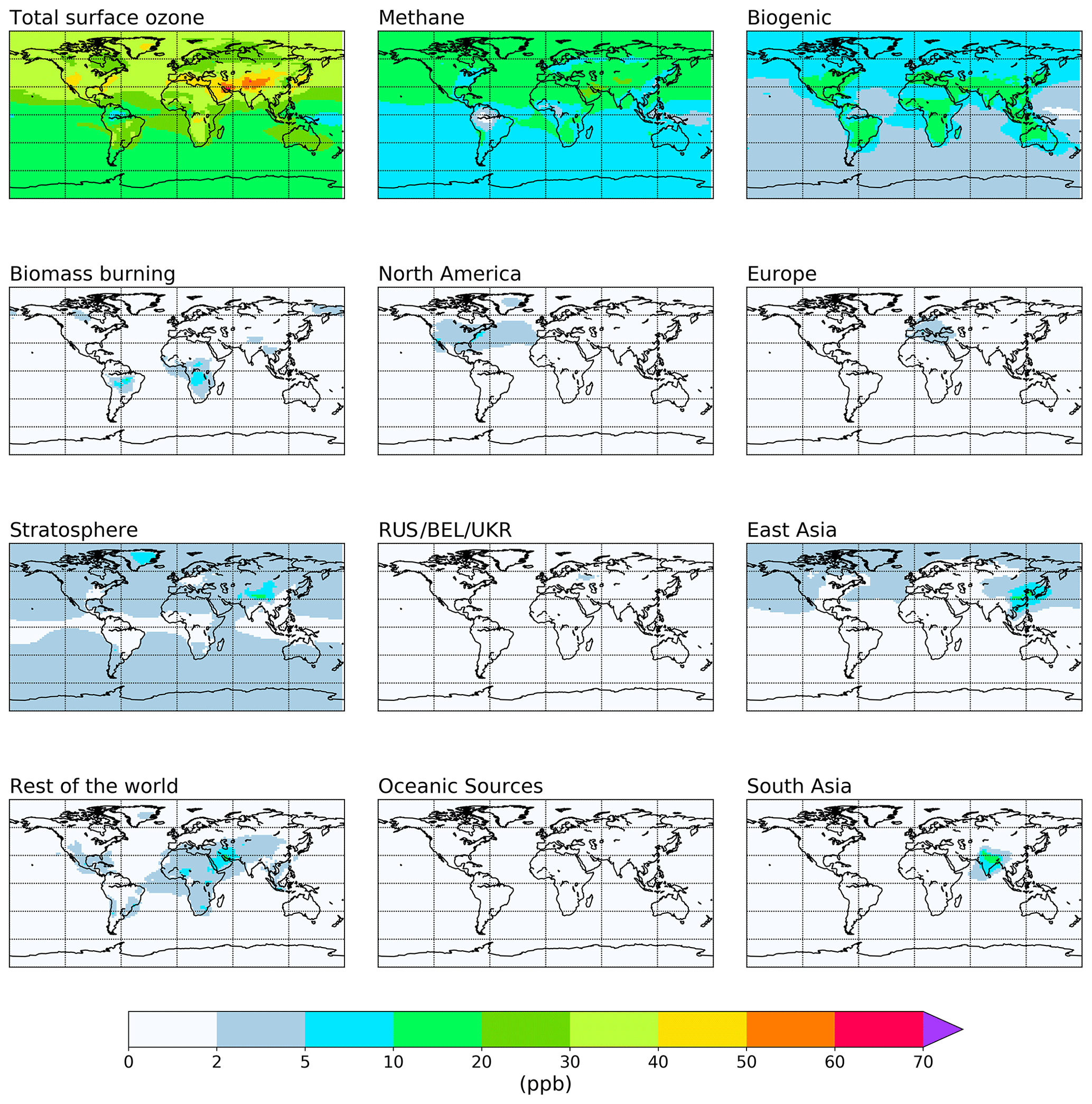
Figure 3 Annual mean surface ozone (ppb) from the VOC-tagged base run. Total ozone is shown in the top left panel. Tagged ozone tracers are shown in the other panels. “RUS/BEL/UKR” refers to Russia, Belarus, and the Ukraine.

Table 2 The attribution of ozone to tagged sources of NO_x. Also shown are the contribution of the stratosphere and the contribution of minor chemical production pathways in the troposphere. Contributions of each tagged source to both the 2010 annual average tropospheric burden and to the annual average Northern Hemisphere (NH) surface mixing ratio are shown. Where applicable, the ozone production efficiency (OPE) of NO_x emissions from each tagged source is also given.

3.1.1 Attribution to NO_x emissions

Anthropogenic NO_x emissions from the three major high-latitude source regions (Europe, East Asia, and North America) contribute to high modelled ozone concentrations both locally and in the Northern Hemisphere background. Lightning NO_x, soil NO_x, and ozone input from the stratosphere all contribute additionally to modelled global background ozone. Emissions of NO_x from shipping contribute significantly to ozone over the major Northern Hemisphere ocean basins, which is also transported over continental regions. South Asia stands out in comparison with the other major Northern Hemisphere source regions in that ozone produced from NO_x emitted in South Asia is relatively localized to the South Asian region itself and is not transported into the hemispheric background to the same extent as ozone produced from NO_x emissions in the other major Northern Hemisphere source regions.

Table 2 shows that NO_x emissions from lightning and aircraft are especially efficient at producing ozone in the free troposphere, consistent with previous work (e.g. Beck et al., 1992; Jacob et al., 1996; Dahlmann et al., 2011). Similarly, surface emissions of NO_x from regions closer to the tropics (e.g. South East Asia and Middle America) produce ozone more effectively due to the rapid convective transport of emitted NO_x into the free troposphere, as shown by Zhang et al. (2016). Of the major Northern Hemisphere source regions, NO_x emissions from South Asia are the most efficient at producing ozone, consistent with a stronger role of vertical transport over this region. In contrast, NO_x emissions from the major anthropogenic source regions in the high northern latitudes (Europe, East Asia, and North America) are among the least productive of all global NO_x emissions, consistent with a relatively small amount of convective transport, leading to higher rates of NO_x removal. Despite their low ozone production efficiency, emissions of NO_x in the high northern latitudes contribute significantly to surface ozone across the Northern Hemisphere (Fig. 2, Table 2).

Table 2 also shows that NO_x emissions from shipping are also relatively efficient at producing ozone, which is also consistent with previous work (e.g. Lawrence and Crutzen, 1999; Hoor et al., 2009). The high ozone production efficiency of ship emissions is due to their location in relatively pristine regions with few other sources of NO_x. Owing to the high ozone productivity of ship emissions and the fact that they are emitted at relatively high latitudes, they contribute significantly to the Northern Hemispheric background (Fig. 2, Table 2). As noted above, the ozone production from ship NO_x is likely to be overestimated due to the artificial dilution of emissions into relatively coarse model grid cells.

Mertens et al. (2018) reported a contribution of shipping to the tropospheric ozone burden of 18 Tg(O₃) using their tagging technique and based on a model simulation with ship NO_x emissions of 6 Tg(N) yr⁻¹. In our study, we calculate a contribution of ship NO_x to tropospheric ozone of 19.9 Tg(O₃) based on ship NO_x emissions of 4.28 Tg(N) yr⁻¹, implying a much higher ozone production efficiency for ship NO_x. As the tagging technique used by Mertens et al. (2018) is based on the method described by Grewe et al. (2017), which combines the effects of tagged NO_x and reactive carbon precursors into a single tagged ozone molecule during ozone production, we do not expect our results to be directly comparable. As shipping emits significantly more NO_x than reactive carbon, we would expect the combinatorial tagging approach of Mertens et al. (2018) to attribute less ozone to shipping than our method, because the ozone produced from ship NO_x would also be partially attributed to the reactive carbon precursor involved in the ozone production. Indeed, Mertens et al. (2018) reported maximum contributions of shipping to surface ozone of about 10 ppb in summer over major Northern Hemisphere ocean basins. In our study, surface ozone attributable to shipping over these regions can exceed 20 ppb (see the Supplement).

3.1.2 Attribution to reactive carbon emissions

Methane and biogenic emissions clearly stand out as major reactive carbon precursors to tropospheric ozone, contributing 35 % and 24 % to the tropospheric ozone burden in our simulation, respectively. Anthropogenic emissions of reactive carbon (excluding biomass burning) together contribute about 14 % to the tropospheric ozone burden. The relatively low influence of anthropogenic reactive carbon emissions on ground-level ozone has been noted elsewhere (e.g. HTAP, 2010; Butler et al., 2018); however, despite this low overall ozone productivity, anthropogenic reactive carbon emissions from source regions in higher northern latitudes still have disproportionately high contributions to surface ozone in the Northern Hemisphere (Table 3).

Table 3 The attribution of ozone to tagged sources of reactive carbon. Also shown are the contribution of the stratosphere and the contribution of minor chemical production pathways in the troposphere. Contributions of each tagged source to both the 2010 annual average tropospheric burden and to the annual average Northern Hemisphere (NH) surface mixing ratio are shown. Where applicable, the ozone production efficiency (OPE) of reactive carbon emissions from each tagged source is also given.

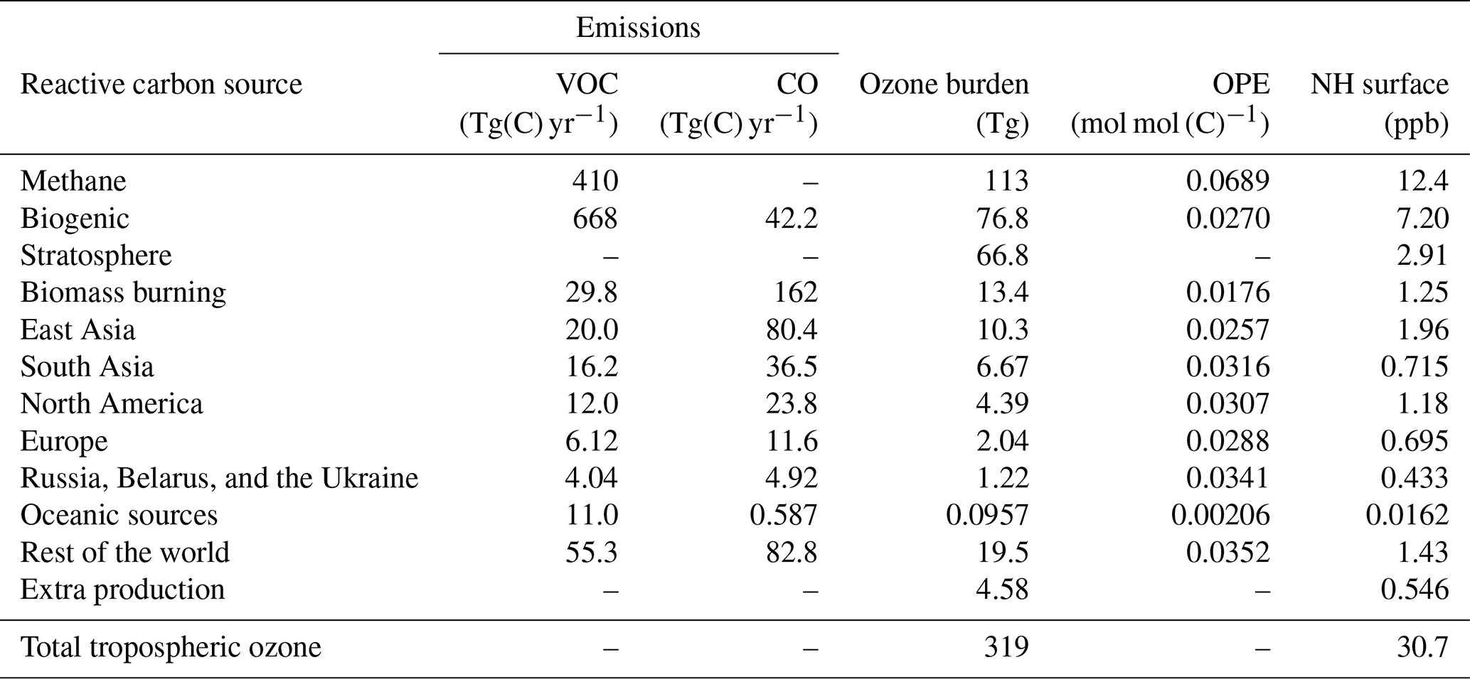
Due to the emissions of CO being tagged together with emitted VOCs in this study, the contribution of each tagged source to the tropospheric ozone burden (and, therefore, also the ozone production efficiency of each tagged source) is a mixture of ozone production due to emitted CO and emitted NMVOCs. The ozone attributed to methane oxidation in Table 3 is due to all stages of methane oxidation in the MOZART-4 chemical mechanism, including the final step in which CO from earlier stages of methane oxidation is itself oxidized to CO₂. The oxidation of CO can produce a maximum of one peroxy radical (HO₂). Therefore, the maximum ozone production potential of CO is 1 mol of ozone per mole of emitted CO. VOCs (including methane) can produce significantly more ozone per mole of emitted carbon, when the subsequent oxidation of the initial oxidation products is taken into account (Bowman and Seinfeld, 1994; Atkinson, 2000; Butler et al., 2011). Future studies using this tagging methodology should consider tagging CO emissions separately from NMVOC emissions if they aim to determine the ozone production efficiency of anthropogenic NMVOC emissions from different world regions. Butler et al. (2018) tagged NMVOC emissions separately from CO emissions, but they did not tag anthropogenic emissions separately according to their geographical region. We re-examined the output of the otherwise identical VOC-tagged run described by Butler et al. (2018) in order to determine the ozone production efficiency of NMVOC emissions from anthropogenic, biomass burning, and biogenic sources: they are 0.0580, 0.0354, and 0.0268 mol(O₃) mol (C)⁻¹ for anthropogenic, biomass burning, and biogenic sources, respectively. The ozone production efficiency of biogenic NMVOCs recalculated from Butler et al. (2018) is not significantly different from the value reported here in Table 3, reflecting the relatively minor contribution of CO to the total amount of emitted biogenic reactive carbon. For biomass burning and anthropogenic sources, however, the ozone production efficiency of NMVOCs emitted from these sources is greater than the corresponding value from Table 3, reflecting the fact that the numbers from Table 3 also include emissions of CO.

We note that methane has a higher ozone production efficiency per unit of reactive carbon (0.0689 mol mol (C)⁻¹; Table 3) than any of the NMVOCs in our runs. The low ozone production efficiency of biogenic NMVOCs is consistent with large amounts of isoprene being emitted in remote regions under low-NO_x conditions, where loss of peroxy radicals through reaction with other peroxy radicals could be expected to dominate (Atkinson, 2000). It might, however, be expected that anthropogenic NMVOCs would have a higher ozone production efficiency, due to the fact that they are co-emitted with anthropogenic NO_x, favouring the conversion of NO to NO₂ via reaction with peroxy radicals and, thus, the production of ozone. The relatively low production efficiency of anthropogenic NMVOCs in our model runs could be due to the fact that the relatively simple chemistry of methane oxidation is well described in the version of the MOZART-4 chemical mechanism used here, in which the relatively complex chemistry of the higher NMVOCs has been simplified. Coates and Butler (2015) noted that the ozone production potential of NMVOCs in simplified chemical mechanisms tended to be lower than the more comprehensive Master Chemical Mechanism (Saunders et al., 2003). Utembe et al. (2010) previously noted increased tropospheric ozone in a CTM when using a more explicit oxidation mechanism for NMVOCs. The extremely low ozone production efficiency of reactive carbon from oceanic sources in Table 3 is due to the lack of any ozone-forming pathways in the oxidation of dimethyl sulfide (DMS) in the MOZART-4 chemical mechanism as used in this study. DMS is the dominant source of reactive carbon over the oceans in our model simulations.

To our knowledge, the only other study to perform source attribution of global tropospheric ozone specifically to reactive carbon precursors is Butler et al. (2018), on which the present study builds. Here, we attribute 113 Tg(O₃) to methane oxidation (Table 3). Grewe et al. (2017) attribute 45 Tg(O₃) to methane using their tagging approach, which combines the effects of tagged NO_x and reactive carbon precursors into a single tagged ozone molecule during ozone production. Ozone production due to methane oxidation under their combinatorial tagging approach would be expected to also include the attribution to the source of NO_x involved in the ozone production. Thus, we would expect Grewe et al. (2017) to attribute approximately half of the amount of ozone to methane that we would. Doubling the value reported by Grewe et al. (2017) yields 90 Tg(O₃) attributable to methane oxidation, which is much closer to our value of 113 Tg.

Widespread implementation of tagging techniques for the separate tagging of NO_x and reactive carbon emissions in other CTMs as well as systematic intercomparisons of their results could help to understand differences in the simulated budgets of tropospheric ozone. Due to the variety of approaches taken by different tagging techniques (summarized in  Butler et al., 2018), an intercomparison of a range of different tagging techniques with other methods for ozone source attribution could be informative.

3.2 Source–receptor relationships for ozone

3.2.1 Annual average surface ozone

Figure 4 shows the modelled annual average surface ozone concentration in the five major HTAP Tier 1 regions in the Northern Hemisphere (Europe; Russia, Belarus, and the Ukraine; South Asia; East Asia; and North America), including a full attribution of ozone in each of these regions to all sources, such as transport from the stratosphere and emitted precursors of both NO_x and reactive carbon. Annual average ozone in most of the regions shown in Fig. 4 is close to the Northern Hemisphere annual average of 30 ppb (Table 2), except in South Asia and East Asia where the annual average surface ozone mixing ratio is closer to 40 ppb. The difference in each case is primarily due to a larger source of ozone produced from locally emitted precursors. Transport from the stratosphere contributes approximately 2–4 ppb to annual average surface ozone depending on the receptor region, which is consistent with the 2.91 ppb contribution of stratospheric ozone to the annual average surface ozone in the Northern Hemisphere average surface ozone (Table 3). As already shown in the previous section, anthropogenic sources of NO_x dominate other NO_x sources as ozone precursors, while the major reactive carbon precursors are methane and biogenic volatile organic compounds (BVOCs).

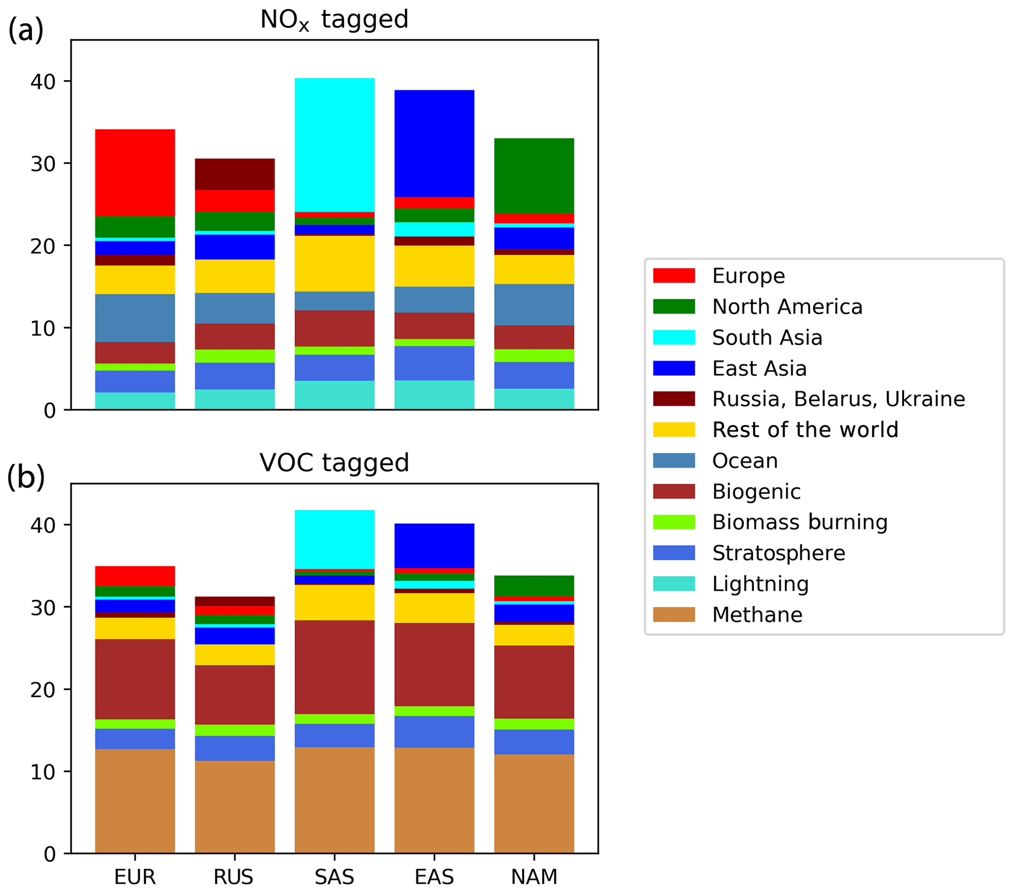
Figure 4 Source–receptor relationships for annual average surface ozone (ppb) in major Northern Hemisphere Tier 1 regions: EUR (Europe), RBU (Russia, Belarus, and the Ukraine), SAS (South Asia), EAS (East Asia), and NAM (North America). The attribution relates the annual average surface ozone modelled in each region to the emitted precursors – NO_x (a) and reactive carbon (b) – from all HTAP Tier 1 regions.

In each of the five regions shown in Fig. 4, natural sources and long-range transport of ozone produced from extra-regional anthropogenic precursors together contribute more to the annual average surface ozone than anthropogenic emissions within the region itself. In each region, the local anthropogenic NO_x emissions produce more ozone than can be attributed to anthropogenic NO_x emissions in any other Tier 1 regions; moreover, with the exception of (South Asia), the combined contribution of external anthropogenic NO_x emissions to annual average surface ozone is greater than the local contribution. The importance of long-range transboundary transport of ozone has also been noted elsewhere (HTAP, 2010).

While anthropogenic precursor emissions from South Asia contribute significantly to surface ozone within the South Asian region, they contribute relatively little to surface ozone in the other four regions shown in Fig. 4. This is also consistent with the surface ozone maps in Fig. 2 and the higher ozone productivity of NO_x emissions from South Asia when compared with the other major Northern Hemisphere source regions (Table 2). Emissions of ozone precursors (particularly NO_x) from South Asia are transported efficiently into the free troposphere, where they contribute disproportionately to the global tropospheric ozone burden (as also noted by Zhang et al., 2016), but the contribution of South Asian emissions to surface ozone in other parts of the Northern Hemisphere is disproportionately smaller than emissions from the other HTAP Tier 1 regions.

3.2.2 Seasonal cycles of surface ozone

Figures 5, 6, and 7 show the seasonal cycles of surface ozone in the three selected Tier 2 regions “North West Europe”, ”North East China”, and “North West United States” respectively. These regions are selected in order to compare two regions on the western side of their respective continents (where long-range transport is expected to be important) with a region on the eastern side of its continent that is also a major source region. A set of figures for other HTAP Tier 2 regions with a complete attribution of surface ozone to all tagged HTAP Tier 1 source regions is available in the Supplement. In Figs. 5, 6, and 7, results are shown for both NO_x and VOC tagging. In each receptor region, the contribution of long-range transport due to extra-regional anthropogenic emissions from HTAP Tier 1 regions is shown both in aggregate (panels a and c) and by individual Tier 1 source region (panels b and d). The definition of the “Rest of the world” ozone tracer has been harmonized between the NO_x- and VOC-tagged runs in these figures. Consistent with the annual averages from Fig. 4, anthropogenic NO_x sources also dominate the seasonal cycle of modelled ozone, while the major reactive carbon precursors of ozone are methane and BVOCs.

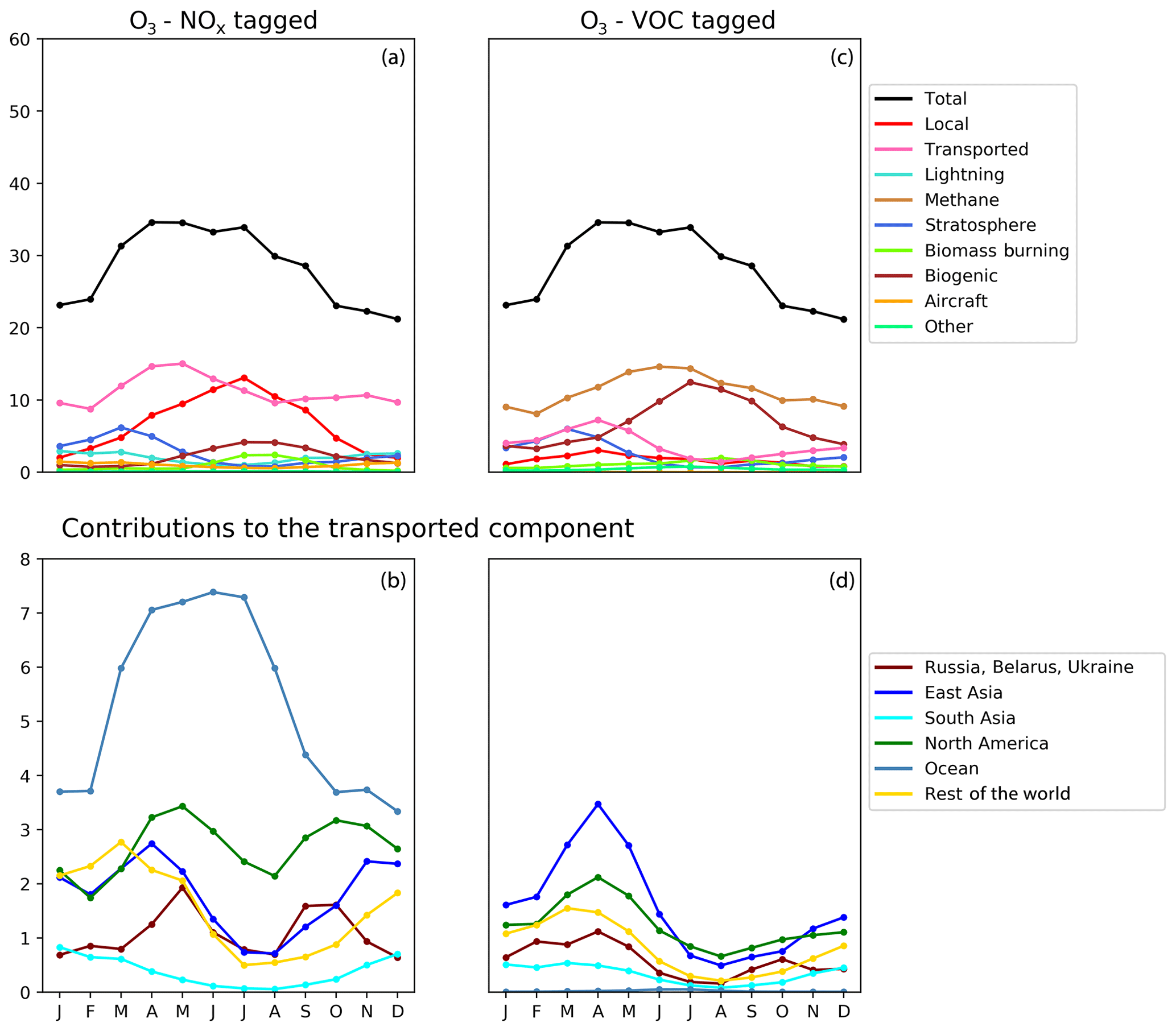
Figure 5 Seasonal cycle of surface ozone (ppb) in the HTAP Tier 2 receptor region “North West Europe”. NO_x tagging is shown in panels (a) and (b), and reactive carbon tagging is shown in panels (c) and (d). Panels (a) and (c) show the total monthly mean ozone (black line) as well as the local anthropogenic component, the long-range transported anthropogenic component, and the natural components. Panels (b) and (d) show the individual Tier 1 source regions responsible for the long-range transported component of ozone.

All three receptor regions show a seasonal cycle of ozone with a spring–summer ozone maximum superimposed on a year-round ozone baseline. The summertime maximum in ozone is clearly due to local photochemical production from the combination of locally emitted anthropogenic NO_x and BVOCs. The strong role of locally emitted precursors in the production of ozone in summer is consistent with earlier work (e.g. Reidmiller et al., 2009; Huang et al., 2017; Jonson et al., 2018; Han et al., 2019), while the importance of BVOC emissions, especially isoprene, for ozone production in summer has also been noted elsewhere (e.g. Chameides et al., 1992; Andersson and Engardt, 2010; Han et al., 2019). Biogenic emissions of NO_x (from soils) also contribute to this summertime maximum in the local photochemical ozone production in all three of the regions shown in Figs. 5, 6, and 7, although to a much smaller extent than anthropogenic NO_x emissions.

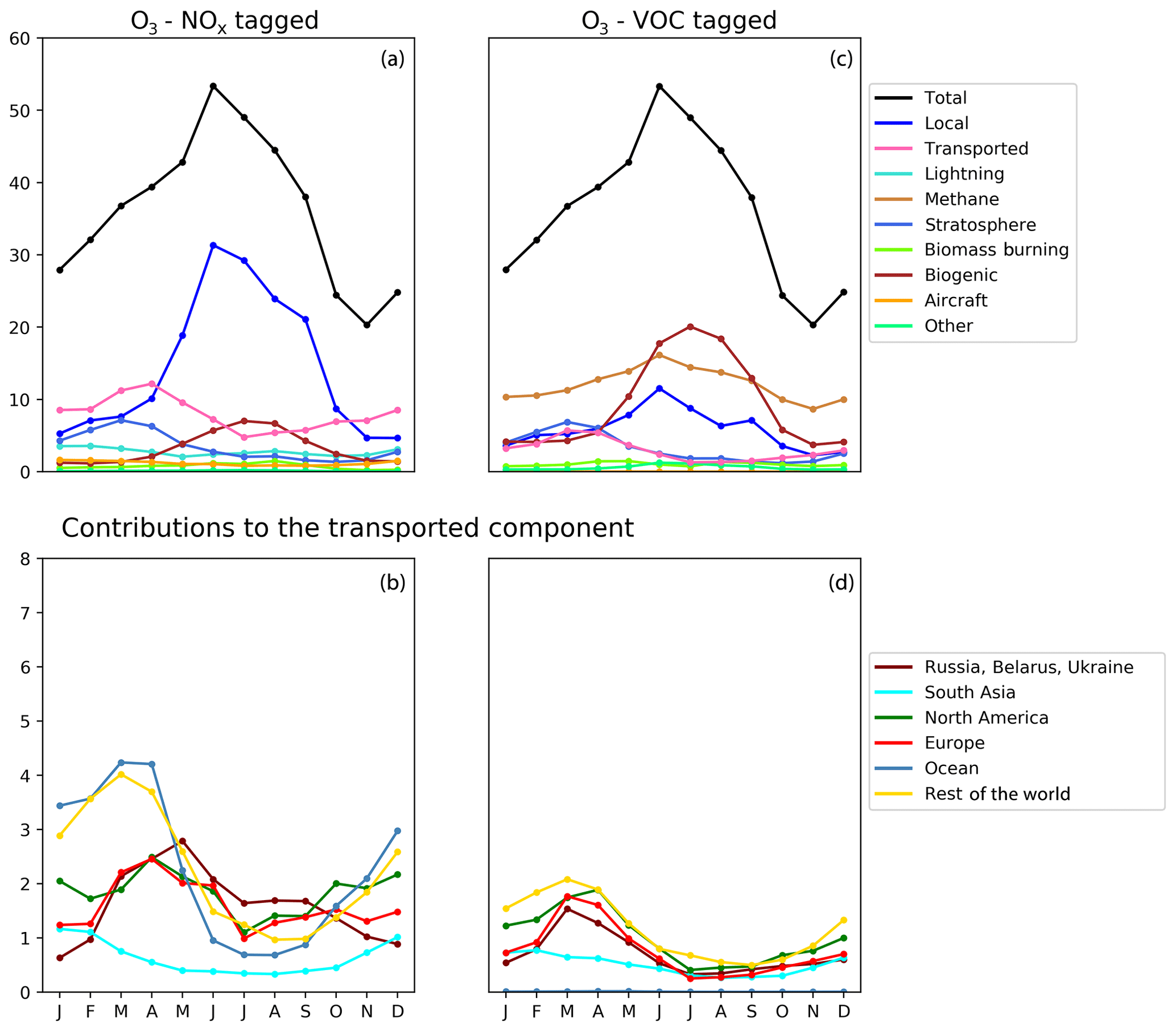
Figure 6 Seasonal cycle of surface ozone (ppb) in the HTAP Tier 2 receptor region “North East China”. NO_x tagging is shown in panels (a) and (b), and reactive carbon tagging is shown in panels (c) and (d). Panels (a) and (c) show the total monthly mean ozone (black line) as well as the local anthropogenic component, the long-range transported anthropogenic component, the and natural components. Panels (b) and (d) show the individual Tier 1 source regions responsible for the long-range transported component of ozone.

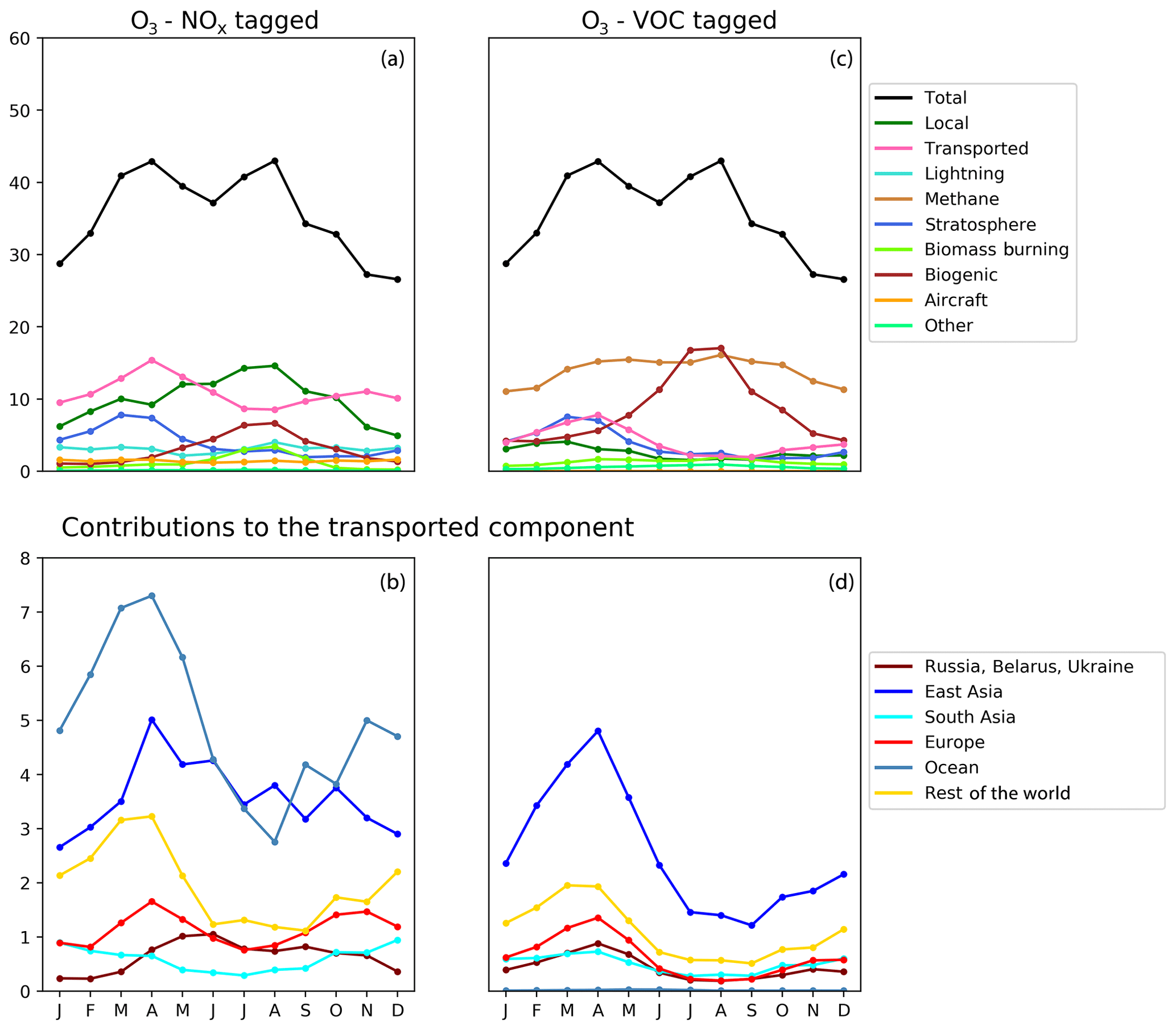
Figure 7 Seasonal cycle of surface ozone (ppb) in the HTAP Tier 2 receptor region “North West United States”. NO_x tagging is shown in panels (a) and (b), and reactive carbon tagging is shown in panels (c) and (d). Panels (a) and (c) show the total monthly mean ozone (black line) as well as the local anthropogenic component, the long-range transported anthropogenic component, and the natural components. Panels (b) and (d) show the individual Tier 1 source regions responsible for the long-range transported component of ozone.

The year-round baseline ozone in our model simulations in all three receptor regions can be primarily explained by slower photochemistry involving methane as the reactive carbon precursor, in combination with extra-regional anthropogenic NO_x (Figs. 5, 6, and 7). The contribution of methane to surface ozone is slightly higher in summer, coinciding with the peak in local anthropogenic NO_x emissions, which is consistent with local photochemical ozone production from enhanced local methane oxidation. The contribution of extra-regional anthropogenic NO_x to surface ozone is largest in spring, coinciding with the peak in the contribution of extra-regional anthropogenic reactive carbon, which is consistent with long-range transboundary transport of ozone produced elsewhere.

Maxima in springtime ozone have previously been linked to long-range transboundary transport in all major receptor regions (HTAP, 2010; Lin et al., 2012; Jonson et al., 2018; Ni et al., 2018). This transported ozone can be attributed to input from the stratosphere as well as extra-regional anthropogenic emissions of NO_x and reactive carbon. In our simulations, the contribution of stratospheric ozone peaks around March, whereas the contribution of extra-regional anthropogenic emissions tends to peak around April, when it contributes more strongly to the monthly average surface ozone in each region than local anthropogenic NO_x (Figs. 5, 6, and 7). In all Northern Hemisphere regions, the springtime peak in the contribution of extra-regional anthropogenic reactive carbon is smaller than the corresponding springtime peak in the contribution of extra-regional anthropogenic NO_x. Previous work has identified uncertainties in the treatment of ozone production from NMVOC oxidation as a potential source of inter-model differences (e.g. Emmerson and Evans, 2009; Utembe et al., 2010; Coates and Butler, 2015). The relatively large influence of anthropogenic NMVOCs on springtime ozone (compared with their influence during other times of the year) could be a contributing factor to the large spread in springtime ozone simulated by current-generation CTMs (Fig. 1).

NO_x from shipping is the largest single contributor to springtime transboundary ozone transport in all three receptor regions shown here. We note, however, that the coarse resolution of our model (2^∘) would be expected to exaggerate the effects of ship NO_x on ozone production due to rapid dilution of the emissions (von Glasow et al., 2003) and exaggerate the transport of NO_x and ozone near coastlines due to unrealistically high diffusion between adjacent land and ocean grid cells. Thus, the contribution of shipping emissions to surface ozone in our simulations should be considered an upper bound, especially in coastal regions. The high contribution of ship NO_x to summertime ozone in Europe (Fig. 5) may be an artefact of the coarse model resolution combined with the high shipping volume near coasts in the eastern North Atlantic Ocean as well as the North Sea. Early work by Lawrence and Crutzen (1999) showed a stronger influence of ship NO_x on surface ozone in northwestern Europe than on any other continental region. Jonson et al. (2018) showed that the only other CTM in the HTAP Phase 2 ensemble to report the results of a perturbation of shipping emissions (the EMEP_rv48 CTM with a resolution of 0.5^∘ × 0.5^∘) shows a similar magnitude for the influence of ship NO_x on summertime ozone in Europe as for springtime ozone. Using a regional model at 50 km ×50 km resolution and a similar ozone tagging system as that used in the present study, Lupaşcu and Butler (2019) showed that the contribution of ship NO_x to ozone in coastal regions of Europe reaches a maximum level in summer. Jonson et al. (2020) used a global model with a resolution of 0.5^∘×0.5^∘ to show that shipping near coastal areas strongly influences ozone over northwestern Europe in both spring and summer, while NO_x emissions from shipping on the high seas have a stronger influence on European ozone in spring than in summer. In contrast, using a higher-resolution regional model (20 km ×20 km) for Europe, Aksoyoglu et al. (2016) did not indicate that ship NO_x played such a strong role in summertime ozone over Europe.

In other receptor regions, the influence of ship NO_x emissions on surface ozone is largest in spring (Figs. 6, 7), suggesting a stronger influence of NO_x emissions over the high seas on springtime ozone in our simulations in these regions. Model-dependent inconsistencies in the treatment of ship NO_x emissions may play a role in the large spread of simulated ozone between models in springtime (Fig. 1). Future work should examine the contribution of ship NO_x emissions to ozone in both spring and summer, using model systems that include the better representations of plume dilution over the major shipping routes, more refined attribution to shipping emissions from coastal regions and the high seas, and higher resolution over receptor regions.

Previous work has indicated a strong influence of anthropogenic emissions from both North America and East Asia on springtime ozone in Europe (Jonson et al., 2018), a strong influence of East Asian emissions on springtime ozone in North America (Lin et al., 2012), and a diverse range of intercontinental influences on springtime ozone in East Asia (Ni et al., 2018). The direct numerical comparison of our results with these previous studies is difficult due to the different methodologies used. These previous studies all employed the perturbation technique to determine the influence of all anthropogenic emissions (both NO_x and reactive carbon) from each source region, whereas this work uses a tagging approach that separately attributes ozone to emitted NO_x and reactive carbon. However, qualitatively, our results (as shown in Figs. 5, 6, and 7) do appear to be consistent with this earlier work. Comparison of the NO_x-tagged and VOC-tagged results in these figures shows that anthropogenic NO_x emissions from most source regions have a stronger influence on springtime ozone in any given receptor region than anthropogenic emissions of reactive carbon. The only exception to this is East Asia, where reactive carbon emissions are substantially higher than in other HTAP Tier 1 source regions (Table 3). Reactive carbon emissions from East Asia contribute approximately equally to springtime ozone in North America when compared to the East Asian NO_x emissions, whereas East Asian reactive carbon contributes more to springtime ozone than East Asian NO_x in Europe.

3.3 Long-range transport of ozone precursors

Fiore et al. (2018) suggested that measurements of the abundance of PAN at mountaintop sites in spring may be useful as an indicator of the intercontinental transport of ozone and its precursors, as well as being a diagnostic for uncertainties in CTM simulations, which show large inter-model differences in simulated PAN (Emmons et al., 2015). The column integrated density of PAN in the lower troposphere (defined here as the model layers between 500 and 800 hPa) in the three HTAP Tier 2 receptor regions “North West Europe”, ”North East China”, and “North West United States” are shown in Figs. 8, 9, 10 respectively. A set of figures for other HTAP Tier 2 regions, with the complete attribution of surface ozone to all tagged HTAP Tier 1 source regions is available in the Supplement. Simulated PAN is highest in late winter to early spring, which is consistent with earlier work (Fischer et al., 2014; Fiore et al., 2018). The extra-regional contribution to PAN is also highest in spring; this is primarily due to anthropogenic NMVOCs, which is also consistent with Fischer et al. (2014).

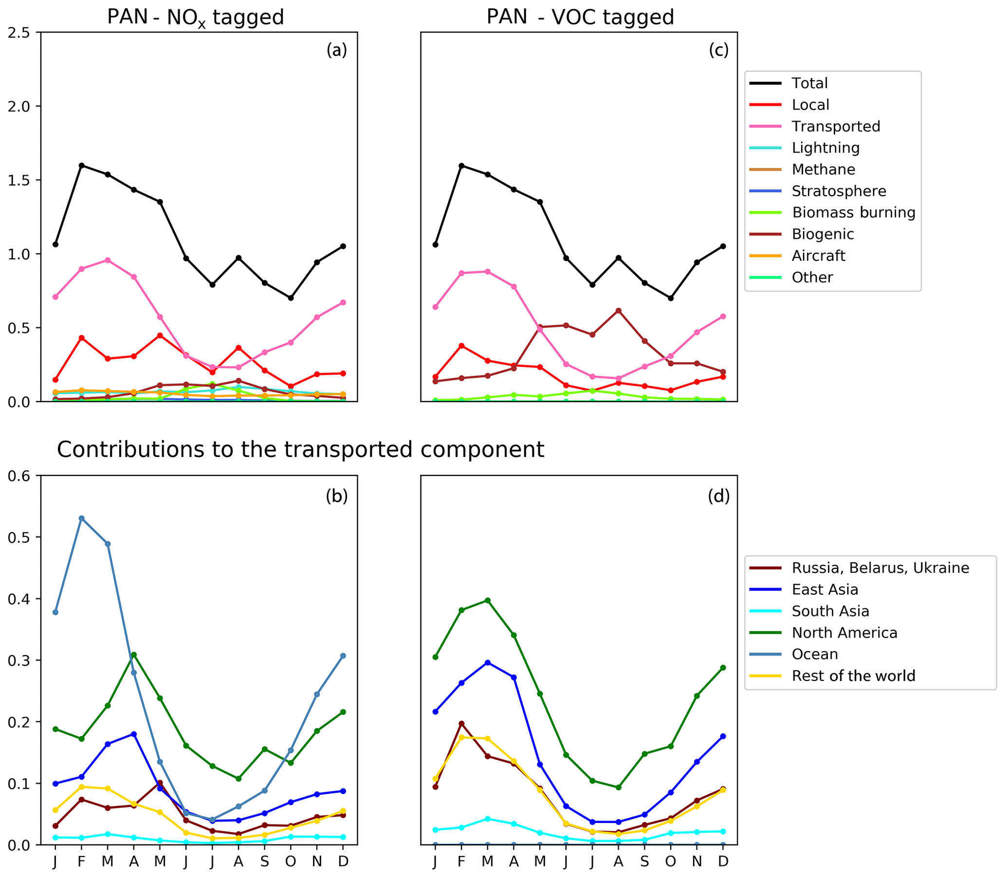
Figure 8 Seasonal cycle of column-integrated lower tropospheric PAN (10⁻¹⁵ molec. cm⁻²) in the HTAP Tier 2 receptor region “North West Europe”. The lower troposphere is defined here as all model levels between 800 and 500 hPa. NO_x tagging is shown in panels (a) and (b), and reactive carbon tagging is shown in panels (c) and (d). Panels (a) and (c) show the total monthly mean PAN (black line) as well as the local anthropogenic component, the long-range transported anthropogenic component, and the natural components. Panels (b) and (d) show the individual Tier 1 source regions responsible for the long-range transported component of PAN.

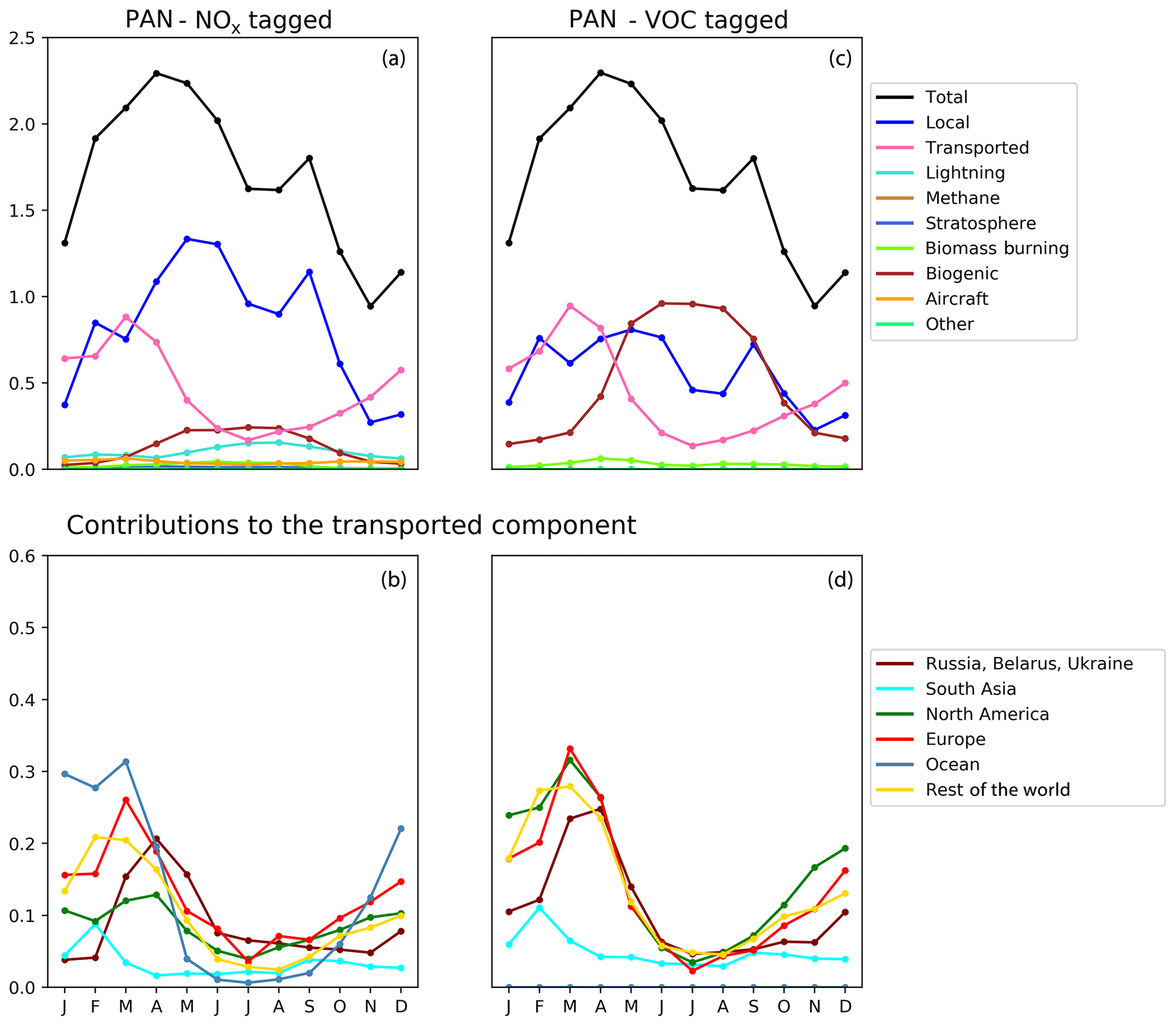
Figure 9 Seasonal cycle of column-integrated lower tropospheric PAN (10⁻¹⁵ molec. cm⁻²) in the HTAP Tier 2 receptor region “North East China”. The lower troposphere is defined here as all model levels between 800 and 500 hPa. NO_x tagging is shown in panels (a) and (b), and reactive carbon tagging is shown in panels (c) and (d). Panels (a) and (c) show total monthly mean PAN (black line) as well as the local anthropogenic component, the long-range transported anthropogenic component, and the natural components. Panels (b) and (d) show the individual Tier 1 source regions responsible for the long-range transported component of PAN.

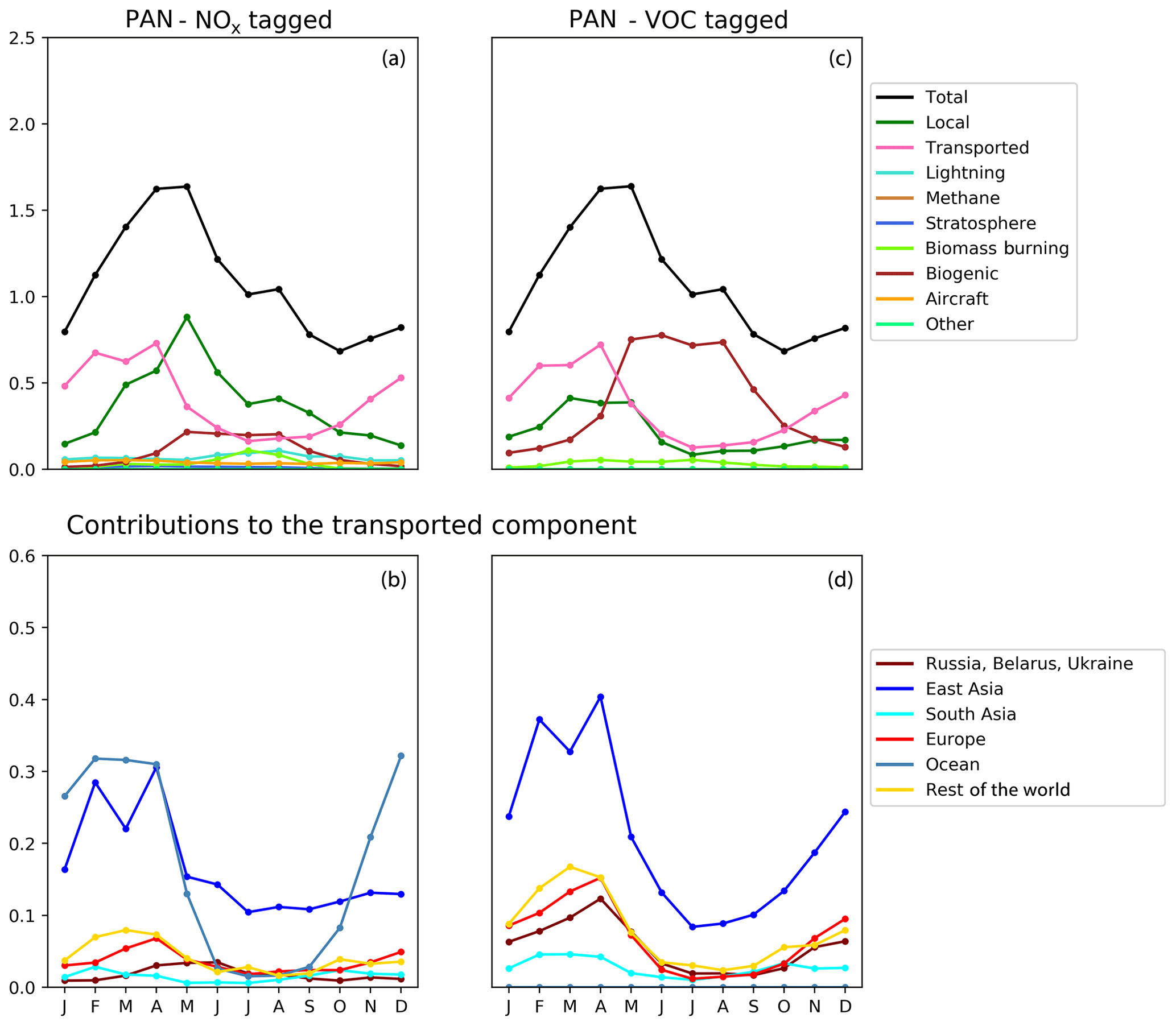
Figure 10 Seasonal cycle of column-integrated lower tropospheric PAN (10⁻¹⁵ molec. cm⁻²) in the HTAP Tier 2 receptor region “North West United States”. The lower troposphere is defined here as all model levels between 800 and 500 hPa. NO_x tagging is shown in panels (a) and (b), and reactive carbon tagging is shown in panels (c) and (d). Panels (a) and (c) show the total monthly mean PAN (black line) as well as the local anthropogenic component, the long-range transported anthropogenic component, and the natural components. Panels (b) and (d) show the individual Tier 1 source regions responsible for the long-range transported component of PAN.

Our model simulations with NO_x and VOC tagging provide a unique opportunity to examine the origin and fate of PAN as simulated in our model, as this allows the simultaneous attribution of simulated PAN to both its NO_x precursor and its reactive carbon precursor. Comparison of panels b and d in Figs. 8, 9, and 10 consistently shows that, for any given land-based HTAP Tier 1 source region, the anthropogenic NMVOC emissions contribute more to PAN formation than the anthropogenic NO_x emissions from that region to the PAN modelled in all HTAP Tier 2 receptor regions. In all cases, the balance of extra-regional PAN is due to NO_x emissions from shipping. In our simulations, significant amounts of PAN are formed downwind of the regions in which the anthropogenic NMVOC precursors are emitted, often via reaction with NO_x emitted from shipping. A strong influence of anthropogenic NO_x emissions on PAN in the northern midlatitudes is consistent with the results shown by Fischer et al. (2014; their Fig. 7, which does not distinguish between different sources of anthropogenic NO_x).

Figures 8, 9, and 10 also show that the reactive carbon component of PAN is generally more persistent than the NO_x component. For example, the contribution of anthropogenic NMVOCs from North America to springtime PAN over East Asia is only slightly lower than its contribution to springtime PAN over Europe, which is much closer to North America considering the prevailing westerly winds (panel d of Figs. 8 and 9). In contrast, the contribution of anthropogenic NO_x from North America to springtime PAN in East Asia is substantially less than its contribution to springtime PAN over Europe (panels b of Figs. 8 and 9).

3.4 Attribution of Northern Hemisphere total organic reactivity

We examine the Northern Hemisphere budget of reactive carbon in more detail in Fig. 11. This figure shows the seasonal cycle of the Northern Hemisphere column-integrated total reactivity with respect to the OH radical of all reactive carbon-containing species in our simulation attributed to their emission source. The total OH reactivity of reactive carbon species of an air mass is often linked to its ozone production potential (Chameides et al., 1992; Kleinman et al., 2002). In each case, the OH reactivities shown in Fig. 11 include the OH reactivity of the primary emitted species as well as the OH reactivity of each carbon-containing oxidation product. These were calculated using the monthly averaged output of the modelled concentration of each carbon-containing species (including its associated tags) and the temperature- and pressure-dependent rate coefficients for their reaction with the OH radical; they were then averaged over all Northern Hemisphere grid cells and weighted by air density.

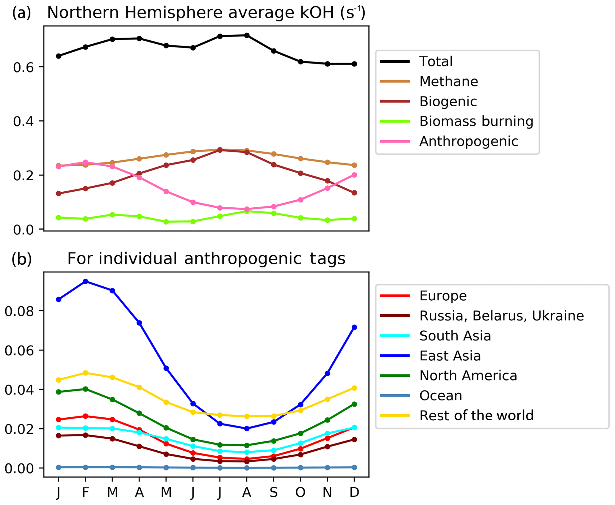
Figure 11 Seasonal cycle of Northern hemispheric tropospheric column-integrated OH reactivity (s⁻¹) due to reactive carbon from the VOC-tagged run. The complete attribution is shown in panel (a), and the detailed attribution to anthropogenic emissions from HTAP Tier 1 source regions is shown in panel (b).

The total Northern Hemisphere OH reactivity of reactive carbon remains fairly constant year-round at about 0.6–0.7 s⁻¹, but the seasonal cycles of the OH reactivity attributable to different reactive carbon sources show more variability. Methane (and its oxidation products) contribute about 0.2–0.3 s⁻¹ (almost half of the total hemispheric reactivity), with a slight maximum in the summer, which is consistent with enhanced oxidation (and, thus, the enhanced availability of more reactive methane oxidation products) due to higher OH in summer. The contributions of anthropogenic and biogenic reactive carbon sources to total hemispheric reactivity are similar, ranging between about 0.1 and 0.3 s⁻¹, but with distinct seasonal cycles. The reactivity of biogenic carbon is highest in summer–autumn (which is consistent with the Northern Hemisphere growing season), whereas the reactivity of anthropogenic carbon is highest in winter–spring (which is consistent with constant year-round anthropogenic emissions and a build-up of reactive carbon over winter due to lower hemispheric OH). The build-up of anthropogenic reactive carbon throughout the Northern Hemisphere over winter combined with the resumption of OH chemistry in spring is consistent with the disproportionate effect of extra-regional anthropogenic reactive carbon on springtime ozone seen in Figs. 5, 6, and 7. Thus, uncertainties in the model chemical mechanisms associated with the oxidation of anthropogenic NMVOCs (e.g. Emmerson and Evans, 2009; Utembe et al., 2010; Coates and Butler, 2015) may also contribute to the large spread in simulated ozone seen in the HTAP ensemble during spring (Fig. 1).

Figure 11 also shows the geographical origin of Northern Hemisphere anthropogenic carbon reactivity. Emissions of reactive carbon from East Asia stand out as the single major source of enhanced anthropogenic carbon reactivity in winter and spring in our simulations. This is consistent with the high emissions of reactive carbon from this region in 2010 noted earlier (Table 3). Growth in NMVOC emissions from East Asia may have continued since this time (Li et al., 2019), while NO_x emissions have been decreasing (Liu et al., 2017). Increasing trends in the local production of ozone during summer over East Asia (e.g. Li et al., 2018) should be associated with the increased oxidation of reactive carbon and, thus, potentially less export of reactive carbon into the Northern Hemisphere background during summer. We expect, however, that increasing emissions of reactive carbon in East Asia could lead to an increased build-up of East Asian reactive carbon in the Northern Hemisphere over winter and, in turn, to an increased East Asian contribution to extra-regional springtime ozone in other parts of the Northern Hemisphere.

Our tagging technique is currently the only one we know of that is capable of examining the budget of reactive carbon in the level of detail presented in this study. The separate tracking of the carbon-containing and nitrogen-containing components of PAN is particularly informative, suggesting that significant amounts of PAN are formed downwind of source regions in our model, especially during winter and spring, due to a build-up of anthropogenic reactive carbon over winter when photochemistry is relatively slow. Given the large variety in model representations of NMVOC chemistry, including PAN formation and decomposition processes (Emmerson and Evans, 2009; Knote et al., 2015) and the large inter-model differences in simulated PAN (Emmons et al., 2015), the widespread implementation of similar tagging diagnostics in other CTMs may help to provide additional information about the origin and fate of simulated PAN and, more generally, about the influence of reactive carbon on atmospheric composition. In combination with routine mountaintop observations of springtime PAN, this may aid understanding of the global PAN budget (Fiore et al., 2018) and other processes responsible for the intercontinental transport of air pollution. Better constraints on these chemical and transport processes should also help to reduce inter-model differences in simulated springtime ozone (Fig. 1).

3.5 Tropospheric ozone sensitivity to methane

We performed an additional set of model runs with both NO_x and VOC tagging with the methane surface boundary condition reduced from 1760 to 1410 ppb, which amounts to a reduction of 350 ppb (or 20 %). This perturbation can also be expressed as an increase of 25 %. Here we interpret the methane perturbation run in terms of the atmospheric response to a 25 % increase in the methane surface mixing ratio at steady state.

In response to the 25 % increase in the imposed surface mixing ratio of methane, the total tropospheric burden increased by 776 Tg(CH₄), which amounts to an increase of 23 %. The strength of the annual tropospheric chemical sink of methane due to OH increased by 72.5 Tg(CH₄) (or 15.2 %). The corresponding increase in the methane lifetime was 0.48 years (or 6.75 %). The relatively small growth in the chemical methane sink compared with the magnitude of the perturbation in methane itself is consistent with the feedback of methane on its own lifetime due to the depletion of OH (Prather, 1996). Table 4 shows the response of the tropospheric ozone burden (and the contributions of different reactive carbon precursors) to the 25 % increase in the imposed surface mixing ratio of methane. The 1 ppb simulated increase in Northern Hemisphere surface ozone in response to a 25 % increase in methane burden is consistent with previous work (HTAP, 2010). The 9.22 Tg increase in tropospheric ozone burden is also consistent with the review of Fiore et al. (2008), who derived a sensitivity of 0.11–0.16 Tg(O₃) per Tg(CH₄) yr⁻¹ emitted based on an analysis of the literature. We calculate 0.13 Tg(O₃) per Tg(CH₄) yr⁻¹ based on our results.

Table 4 Change in the contribution of reactive carbon sources to tropospheric and Northern Hemisphere (NH) surface ozone in response to a 25 % increase in the imposed surface mixing ratio of methane. Absolute changes and percentage changes are both shown.

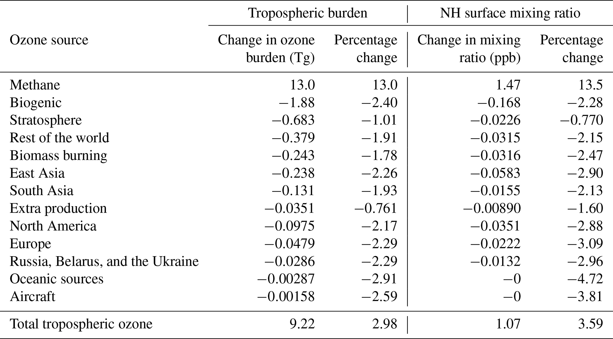
The relative increase in tropospheric ozone attributed to methane (13.0 %) by our tagging scheme is comparable to, but slightly smaller than, the increase in the magnitude of the chemical methane sink due to OH (15.2 %), which is consistent with the troposphere as a whole becoming slightly more NO_x limited with increasing methane. The absolute increase in the total ozone burden (9.22 Tg(O₃)) is, however, significantly lower than the increase in the burden of ozone attributed to methane by our tagging scheme (13.0 Tg(O₃)). When the methane burden is increased, the contribution of every other reactive carbon source to the tropospheric ozone burden decreases (each by approximately 1 %–2 %) to partially offset the increased ozone production from methane oxidation. This is also consistent with a slightly more NO_x-limited atmosphere with increasing methane. In a future with an increased methane burden, control of NMVOC emissions could be expected to be less effective at the large-scale reduction of annual average ground-level ozone.

Table 5 shows the change in the contributions of different NO_x sources to tropospheric ozone in response to the 25 % increase in the methane burden. As expected, all NO_x sources become more productive when the total atmospheric burden of reactive carbon is increased (which is consistent with the troposphere as a whole becoming more NO_x limited). The increase in the productivity of the different NO_x sources under an increased burden of methane is, however, not uniform. Ozone production due to NO_x from shipping stands out as highly sensitive to the global methane burden in our simulations. Ship NO_x accounts for almost 30 % of the 1 ppb increase in Northern Hemisphere average surface ozone when the methane burden is increased by 25 % (Table 5), despite being a much smaller percentage of total global NO_x emissions (Table 2).

Table 5 Change in the contribution of NO_x sources to tropospheric and Northern Hemisphere surface ozone in response to a 25 % increase in the imposed surface mixing ratio of methane. Absolute changes and percentage changes are both shown.

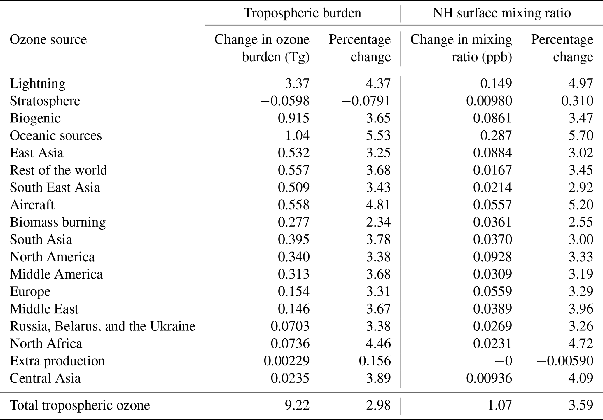
The spatial distribution of the increase in annual average surface ozone from ship NO_x in response to the 25 % increase in methane is similar to the spatial distribution of surface ozone due to ship NO_x in our base run (Fig. 2). Figures showing the response of the attributed surface ozone are available in the Supplement. The response is largest over the major Northern Hemisphere ocean basins, but it also extends over continental regions. The seasonal cycle of the increase in annual average surface ozone from ship NO_x in the three HTAP Tier 2 regions examined here in response to the 25 % increase in methane is similar to the seasonal cycle of surface ozone due to ship NO_x in our base run (Figs. 5, 6, and 7). The maximum response of surface ozone from ship NO_x to rising methane is simulated over the major Northern Hemisphere ocean basins in summer (which influences surface ozone in northwestern Europe in our simulations; Fig. 5), while the influence of this response over most Northern Hemisphere continental regions is generally higher in winter–spring (as seen in northeastern China; Fig. 6).

Previous work (Lawrence and Crutzen, 1999) has noted the disproportionate influence of ship NO_x on tropospheric ozone due to the diffuse and widespread nature of this source over regions that would otherwise have very low NO_x mixing ratios. Fiore et al. (2008) noted that the response of surface ozone to increased methane was especially strong in ship tracks. Myhre et al. (2011) also showed that ship NO_x emissions reduce the global methane lifetime much more than terrestrial NO_x emissions. We note again that the contribution of ship NO_x to ozone in our simulations (as in most current-generation CTMs) is likely to be an overestimate due to the unrealistic dilution of these emissions into coarse model grid cells (von Glasow et al., 2003) and the lack of explicit plume chemistry (Vinken et al., 2011). However, we do expect that the interaction between ship NO_x and methane for ozone production would persist in our model even with a more realistic treatment of ship emissions, as this interaction is likely due to the location rather than the magnitude of ship emissions. We are not aware of any previous work linking the combined influence of these two sources to a potentially disproportionate influence on background ozone in the Northern Hemisphere or on modelled surface ozone air quality in inhabited regions of the Northern Hemisphere, especially in spring. Given the current uncertainty in the attribution of recent trends in methane (Turner et al., 2019) and the potential for future increases in methane emissions, combined with slower reductions of NO_x emissions from international shipping than from other sectors (e.g. the SSP5 future emission scenario Rao et al., 2017), we expect that model simulations of future background ozone in the Northern Hemisphere, especially during spring, may come to be increasingly influenced by ozone produced via the interaction of methane and ship NO_x. Future work should investigate the ozone production via the interaction of these two sources in more detail.

4 Conclusions

We have performed a source attribution for tropospheric ozone in a chemical transport model using a novel technique that separately accounts for the influence of both the emitted NO_x and the emitted reactive carbon precursors on simulated tropospheric ozone. By tagging anthropogenic emissions of NO_x and reactive carbon according to their geographical region, we have calculated source–receptor relationships for the Northern Hemisphere. The results of our study are consistent with previous work, and they provide a number of important new insights that are relevant to both the mitigation of intercontinental transboundary air pollution and ongoing efforts to reduce the uncertainty in the current generation of chemical transport models.

Consistent with previous work, the annual average ground-level ozone in all major Northern Hemisphere regions is primarily influenced by extra-regional emissions of both NO_x and reactive carbon. In all cases, local anthropogenic emissions of ozone precursors have a smaller influence on annual average ozone than the combined effect of precursor emissions from the rest of the world. As a reactive carbon precursor, methane contributes 35 % of the tropospheric ozone burden and 41 % of the Northern Hemisphere annual average surface mixing ratio, which is more than any other source of reactive carbon. Our novel tagging methodology also reproduces the well-known dependence of summer ozone maxima on local emissions of anthropogenic NO_x and biogenic reactive carbon as well as the enhanced importance of the intercontinental transport of ozone from remote anthropogenic sources in spring. Consistent with previous work, we find that emissions of NO_x at low latitudes produce free-tropospheric ozone more effectively due to more efficient vertical transport. We show, however, that NO_x sources at higher northern latitudes have a stronger influence on ground-level ozone, which is known to have a lower radiative forcing but a higher influence on human health and ecosystems.

The current generation of chemical transport models has particular difficulty simulating the intercontinental transport of ozone, as shown by the large spread in ensemble simulations of ground-level ozone during the spring months. We show that our tagging methodology can deliver detailed diagnostic information about the origin and budget of springtime ozone in our model, along with information about the springtime budget of peroxyacetyl nitrate (PAN), which is also associated with springtime long-range transport and ozone production. We show that a substantial proportion of the free-tropospheric PAN simulated by our model in spring is not produced in the polluted boundary layer over the major anthropogenic source regions; instead, it is produced downwind of these regions in our model via the interaction of transported anthropogenic reactive carbon and NO_x emitted from international shipping. Reactive carbon of anthropogenic origin (and its oxidation products, including PAN) builds up in our model across the entire Northern Hemisphere during the winter months and then contributes to a short burst of hemispheric-scale ozone production during spring in our simulations. In all but the most polluted source regions, anthropogenic NMVOCs do not make a significant contribution to simulated ground level ozone in any other season but spring.

In this study, we showed that the export of anthropogenic reactive carbon from East Asia may be playing a dominant role in contributing to the build-up of reactive carbon in the Northern Hemisphere over winter and, in turn, to the hemispheric-scale production of ground-level ozone in spring. Given the likely lack of recent mitigation in reactive carbon emissions from East Asia, we expect this effect to be ongoing, and we recommend that future work continue to investigate this possibility using updated emission inventories.

In addition to a contribution from the stratosphere, the springtime peak in transported ozone in our model is influenced by the interaction of two processes known to be especially poorly represented in current models: the chemistry of the intermediate oxidation products of NMVOCs and the emissions of NO_x from international shipping. Furthermore, the response of ground-level ozone to changes in methane also appears highly sensitive to the treatment of ship NO_x, especially in spring. We believe that our tagging technique could deliver useful information about the large differences in simulated springtime ozone between current-generation models if it were to be implemented in a larger number of models and used systematically in model intercomparison exercises. This could potentially point the way to improved representations of the processes responsible for the intercontinental transport of ozone.

Improved global CTMs are required to inform effective policies aimed at reducing the intercontinental transport of ground-level ozone – a problem which is most urgent in the springtime. In particular, we recommend that developers of emission inventories and CTMs revisit their representations of anthropogenic NMVOC emissions and the associated oxidation chemistry in order to reduce the uncertainties in the modelled springtime ozone. Additionally, more explicit representations of the NO_x chemistry of ship exhaust plumes should be prioritized in order to improve the suitability of the current models for simulating both the intercontinental transport of ozone and the response of ozone to changing atmospheric methane.