Comparing secondary organic aerosol (SOA) volatility distributions derived from isothermal SOA particle evaporation data and FIGAERO–CIMS measurements

The volatility distribution of the organic compounds present in secondary organic aerosol (SOA) at different conditions is a key quantity that has to be captured in order to describe SOA dynamics accurately. The development of the Filter Inlet for Gases and AEROsols (FIGAERO) and its coupling to a chemical ionization mass spectrometer (CIMS; collectively FIGAERO–CIMS) has enabled near-simultaneous sampling of the gas and particle phases of SOA through thermal desorption of the particles. The thermal desorption data have been recently shown to be interpretable as a volatility distribution with the use of the positive matrix factorization (PMF) method. Similarly, volatility distributions can be inferred from isothermal particle evaporation experiments when the particle size change measurements are analyzed with process-modeling techniques. In this study, we compare the volatility distributions that are retrieved from FIGAERO–CIMS and particle size change measurements during isothermal particle evaporation with process-modeling techniques. We compare the volatility distributions at two different relative humidities (RHs) and two oxidation conditions. In high-RH conditions, where particles are in a liquid state, we show that the volatility distributions derived via the two ways are similar within a reasonable assumption of uncertainty in the effective saturation mass concentrations that are derived from FIGAERO–CIMS data. In dry conditions, we demonstrate that the volatility distributions are comparable in one oxidation condition, and in the other oxidation condition, the volatility distribution derived from the PMF analysis shows considerably more high-volatility matter than the volatility distribution inferred from particle size change measurements. We also show that the Vogel–Tammann–Fulcher equation together with a recent glass transition temperature parametrization for organic compounds and PMF-derived volatility distribution estimates are consistent with the observed isothermal evaporation under dry conditions within the reported uncertainties. We conclude that the FIGAERO–CIMS measurements analyzed with the PMF method are a promising method for inferring the volatility distribution of organic compounds, but care has to be taken when the PMF factors are analyzed. Future process-modeling studies about SOA dynamics and properties could benefit from simultaneous FIGAERO–CIMS measurements.

1 Introduction

Aerosol particles have varying effects on health, visibility and climate (Stocker et al., 2013). Organic compounds comprise a substantial amount of atmospheric particulate matter (Jimenez et al., 2009; Zhang et al., 2007) of which a major fraction is of secondary origin, i.e., low-volatility organic compounds formed from oxidation reactions between volatile organic compounds (VOCs) and ozone, hydroxyl radicals and nitrate radicals (Hallquist et al., 2009). The aerosol particles containing these kind of oxidation products are called secondary organic aerosols (SOAs) as opposed to primary organic aerosols, i.e., organic particles emitted directly to the atmosphere. VOC oxidation reactions result in thousands of different organic compounds (Goldstein and Galbally, 2007). There are gaps in the knowledge, especially on the formation and deposition of SOAs and how the processes are affected by changing physicochemical properties such as volatility (Glasius and Goldstein, 2016). In addition, the phase state of the organic compounds has also been shown to play a role in SOA dynamics (Reid et al., 2018; Shiraiwa et al., 2017; Yli-Juuti et al., 2017; Renbaum-Wolff et al., 2013; Virtanen et al., 2010)

The physicochemical properties of organic aerosols can be studied directly and indirectly. The Aerodyne aerosol mass spectrometer (AMS; Canagaratna et al., 2007; DeCarlo et al., 2006; Jayne et al., 2000) enabled direct and online composition measurements of atmospheric particles for the first time. Combining AMS data with statistical dimension reduction techniques such as factor analysis and positive matrix factorization (PMF; Zhang et al., 2011, 2007, 2005; Paatero and Tapper, 1994) allowed researchers to draw conclusions on sources and types of atmospheric organic particulate matter from the relatively complex mass spectra data.

The chemical ionization mass spectrometer (CIMS; Lee et al., 2014) coupled with the Filter Inlet for Gases and AEROsols (FIGAERO, collectively FIGAERO–CIMS; Lopez-Hilfiker et al., 2014) is a prominent online measurement device for studying both the gas and particle phases of SOAs. During particle-phase measurements, a key advantage over the AMS is the softer chemical ionization that retains much more of the molecular information of the compound than the electron impact ionization used in the AMS. Typically, the collection of the particulate mass is conducted at room temperature, which minimizes the loss of semivolatile compounds during collection. In addition to the overall chemical composition, the gradual desorption of the particulate mass from the FIGAERO filter yields the thermal desorption behavior of each detected ion, i.e., it is a direct measurement of each ion's volatility. FIGAERO–CIMS measurements have been carried out in both laboratory and field environments to study SOA composition from different VOC precursors and in both rural and polluted environments (Le Breton et al., 2018; Huang et al., 2018; Lee et al., 2018; D'Ambro et al., 2017; Lopez-Hilfiker et al., 2015). However, the volatility information in these data sets has barely been used.

Besides direct mass spectrometer measurements, SOA properties have been inferred indirectly from growth (e.g., Pathak et al., 2007 and references therein) and isothermal evaporation (Buchholz et al., 2019; D'Ambro et al., 2018; Yli-Juuti et al., 2017; Wilson et al., 2015; Vaden et al., 2011) measurements. The complexity of organic compounds in these studies can be alleviated with the use of a volatility basis set (Donahue et al., 2006), where organic compounds are grouped based on their (effective) saturation concentration. However, the experimental setup also defines the range of C^∗ values that can be estimated from the data. Vaden et al. (2011) and Yli-Juuti et al. (2017) have both shown that the volatility basis sets derived from SOA growth experiments result in too fast an SOA evaporation compared to measured evaporation rates when the volatility basis set is used as input for process models. Possible reasons for such discrepancies include the different C^∗ ranges to which the SOA growth and SOA evaporation experiments are sensitive and the role of vapor wall losses in SOA growth experiments. This raises a need for alternative methods to derive organic aerosol volatility against which the volatilities inferred from the direct particle size measurements can be compared.

Recently, Buchholz et al. (2020) demonstrated that the FIGAERO–CIMS measurements during particle evaporation can be mapped to a volatility distribution of organic compounds by conducting a PMF analysis. On the other hand, Tikkanen et al. (2019) showed that the volatility distribution can be inferred from isothermal particle evaporation measurements by optimizing the evaporation model input to yield the measured evaporation rate at different humidity conditions. In this study, we compare these two approaches for varying oxidation and particle water content conditions. Our main research questions are as follows. (1) Are the volatility distributions derived from particle size change during isothermal evaporation and from the FIGAERO–CIMS measurements similar? (2) How should the PMF results of FIGAERO–CIMS data be interpreted in terms of volatility? (3) Can a recently published glass transition temperature parametrization (DeRieux et al., 2018), combined with the PMF analysis, be used to model particle-phase mass transfer limitations observed for the evaporation in dry conditions, i.e., in the absence of particle-phase water?

2 Methods

2.1 Experimental particle evaporation data

The experimental data we use are the same as reported in Buchholz et al. (2019, 2020). We briefly summarize the measurement setup below. We generated the particles with a potential aerosol mass (PAM) reactor (Kang et al., 2007; Lambe et al., 2011) from the reaction of α-pinene with O₃ and OH at three different oxidation levels (average oxygen-to-carbon (O:C) ratios of 0.53, 0.69 and 0.96). We focus on the lowest O:C (0.53) and medium-O:C (0.69) experiments in this work. The closer analysis of the high-O:C experiments suggests particle-phase reactions during the evaporation (Buchholz et al., 2019, 2020). To avoid the uncertainty that would arise from unknown particle-phase reactions, we chose not to include the high-O:C data in our analysis.

We selected a monodisperse particle population (mobility diameter d_p = 80 nm) with two nano-tandem-type differential mobility analyzers (nano-DMA; TSI Incorporated, model 3085) from the initial polydisperse particle population. The size selection diluted the gas phase, initiating particle evaporation. The monodisperse aerosol was left to evaporate in a 100 L stainless-steel residence time chamber (RTC). We measured the particle size distribution during the evaporation with a scanning mobility particle sizer (SMPS; TSI Incorporated, models 3082 and 3775). The RTC filling took approximately 20 min, and we performed the first size-distribution measurement in the middle of the filling interval. To obtain short residence time data (data before 10 min of evaporation) we added a bypass to the RTC, which led the sample directly to the SMPS. By changing the length of the bypass tubing, we were able to measure the particle size distribution between 2 and 160 s of evaporation. We measured the isothermal evaporation up to 4–10 h, depending on the measurement. We performed the measurements for each oxidation level both at high relative humidity (RH = 80 %) and at dry conditions (RH < 2 %). The change in particle size with respect to time is called an evapogram. In an evapogram, the horizontal axis presents evaporation time, and the vertical axis shows the evaporation factor (EF), i.e., the measured particle diameter divided by the initially selected particle diameter.

To classify the oxidation level of the particles, we derived the average O:C ratio from composition measurements with a high-resolution time-of-flight aerosol mass spectrometer (AMS; Aerodyne Research, Inc.). Furthermore, we conducted detailed particle composition measurements with an Aerodyne Research, Inc. FIGAERO (Lopez-Hilfiker et al., 2014) coupled with a chemical ionization mass spectrometer (CIMS), with iodide as the reagent ion (Aerodyne Research Inc.; Lee et al., 2014). Previous studies using FIGAERO–CIMS with iodide as the reagent ion found 50 % or better mass closure compared to more established methods of quantifying organic aerosol (OA) mass (albeit with high uncertainties; Isaacman-VanWertz et al., 2017; Lopez-Hilfiker et al., 2016). Therefore, it appears that the bulk of reaction products expected from α-pinene oxidation contains the functional groups required for detection by our FIGAERO–CIMS.

In the FIGAERO inlet, particles are first collected on a polytetrafluoroethylene (PTFE) filter. Then the collected particulate mass desorbs slowly due to a gradually heated nitrogen flow. The desorbed gaseous compounds are then transported into the CIMS for detection. We derived the average chemical composition of the particles by integrating the detected signal of each ion over the whole desorption interval. For each ion, the change in detected signal with desorption temperature is called a thermogram, and generally, the temperature at the maximum of the thermogram (T_max) is correlated to the volatility of the detected ion. Similar to Bannan et al. (2019) and Stark et al. (2017), we calibrated the T_max–volatility relationship using compounds with known vapor pressure. The calibration procedure is described in the Supplement.

We collected particles for FIGAERO–CIMS analysis at two different stages of the evaporation. We refer to these samples as either “fresh” or “RTC” samples. The fresh samples were collected for 30 min directly after the selection of the monodisperse population. The RTC samples of the residual particles were collected for 75 min after 3–4 h of evaporation in the RTC. The collected particulate mass was 140–260 and 20–70 ng for the fresh and the RTC samples, respectively. More details about sample collection, desorption parameters and data analysis can be found in Buchholz et al. (2020).

2.2 The volatility distribution

We represent the myriad of organic compound in the SOA particles with a one-dimensional volatility basis set (1D VBS; below only VBS; Donahue et al., 2006). The VBS groups the organic compounds into “bins” based on their effective (mass) saturation concentration C^∗, defined as the product of the compounds' activity coefficient and saturation concentration. Generally, a bin in the VBS represents the amount of organic material in the particle and gas phases. In our study, the walls of the RTC have been shown to work as an efficient sink for gaseous organic compounds (Yli-Juuti et al., 2017). Thus, we can assume that the gas phase in our experimental setup does not contain organic compounds, i.e., the amount of organic matter in a bin is the amount in the particle phase. To distinguish from a traditional VBS that groups the organic compounds to bins such that there is a decadal difference in C^∗ between two adjacent bins, we call the VBS in our work a volatility distribution (VD). We present the amount of material in each VD bin as the dry mole fraction, i.e., the mole fraction of the organics, excluding water. In the analysis presented below, we assign properties to each VD bin (e.g., molar mass), treating each bin as if it consisted of only a single organic compound with a single set of properties. The physicochemical properties of each VD bin are assumed to be the same. These properties and the ambient conditions of each evaporation experiment are listed in Table 1.

Table 1 The ambient conditions and properties of the organic compounds used in estimating the VD_evap. The variables are, from top to bottom, temperature (T) during the evaporation, relative humidity (RH), gas-phase diffusion coefficient (D_g,org), molar mass (M), particle-phase density (ρ), particle surface tension (σ) and mass accommodation coefficient (α). Rows that only have one value are the same in every column.

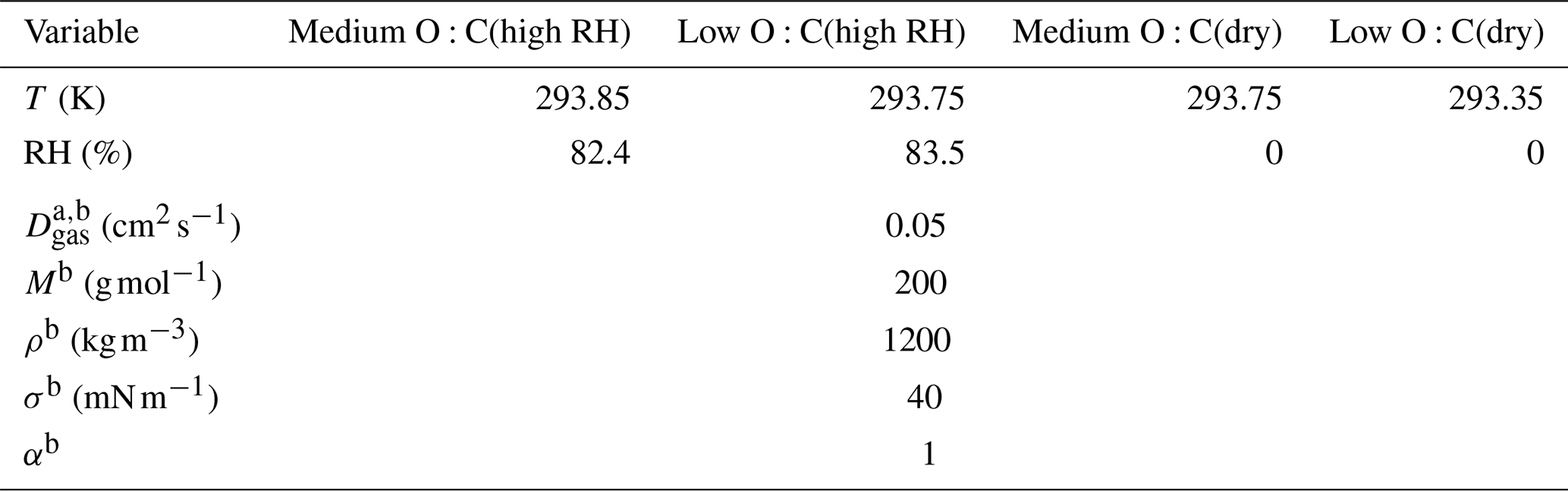
^a The gas-phase diffusion coefficients are scaled to correct the temperatures by multiplying with a factor of (T∕273.15)^1.75 (Reid et al., 1987).
^b Values are chosen to represent a generic organic compound with values similar to other α-pinene SOA studies (e.g., Pathak et al., 2007; Vaden et al., 2011; Yli-Juuti et al., 2017).

2.3 Deriving volatility distribution from an evapogram

We followed a similar approach as in Yli-Juuti et al. (2017) and Tikkanen et al. (2019) to derive a VD at the start of the evaporation from an evapogram. To model the evaporation at high RH, we used a process model (liquid-like evaporation model, hereafter LLEVAP) that assumes a liquid-like particle, i.e., a particle in which there are no mass transfer limitations inside the particle and where the mass flux of a VD bin in the particle phase can be calculated directly from the gas-phase concentrations of the VD bin both near the particle surface and far away from the particle (Vesala et al., 1997; Lehtinen and Kulmala, 2003; Yli-Juuti et al., 2017). In this case, the main properties for defining the evaporation rate are the saturation concentrations of each VD bin and their relative amounts in the particle.

We used the LLEVAP model to characterize the volatility range that can be interpreted from the evaporation measurements. We calculated the range by modeling the evaporation of a hypothetical particle that consists of one organic compound evaporating in dry conditions. We calculated the evaporation for the range of log₁₀(C^∗) values from −5 to 5. We determined the minimum C^∗ value to be the value that still showed “detectable evaporation”, i.e., at least 1 % change in particle diameter during the evaporation time (up to 6 h), and the maximum C^∗ value to be the value before “complete evaporation” occurred, i.e., 99 % particle diameter change within the first 10 s. The minimum log₁₀ (C^∗) calculated with this method was −3 and the maximum log₁₀ (C^∗) was 2. We then modeled the particle composition with six VD bins with C^∗ values between these minimum and maximum values. Each VD bin has a decadal difference in C^∗ to an adjacent VD bin (like in the traditional VBS). We note that, based on this analysis, all the compounds with log₁₀ (C^∗) < −3 will not evaporate during the experimental timescale. This means that any compounds with lower C^∗ than this threshold will be assigned to the log₁₀ (C^∗) = −3 VD bin. Similarly, any compound with log₁₀ (C^∗) > 2 will be classified into the log₁₀ (C^∗) = 2 VD bin or not be detected at all due to evaporating almost entirely before the first measurement point.

We calculated the dry particle mole fraction of each VD bin at the start of the evaporation by fitting the evaporation predicted with the process model to the measured evapograms. Our goal was to minimize the mean squared error in a vertical direction between the experimental data and the LLEVAP output. We used the Monte Carlo genetic algorithm (MCGA; Berkemeier et al., 2017; Tikkanen et al., 2019) for the input optimization. In the optimization, we set the population size to be 400 candidates, number of elite members to 20 (5 % of the population), number of generations to 10 and number of candidates drawn in the Monte Carlo (MC) part to 3420, which corresponds to half of the total process model evaluations done during the optimization. We performed the optimization 50 times for each evapogram and selected the best-fit VD estimate for further analysis.

The VD derived from the evapogram is hereafter referred to as the VD_evap. The initial composition of the SOA particles in the dry and wet experiments was the same and can be described by the same fitted VD_evap as the particles were generated at the same conditions in the PAM and only the evaporation conditions changed.

2.4 Deriving volatility distribution from FIGAERO–CIMS measurement

As shown by Bannan et al. (2019) and Stark et al. (2017), the peak desorption temperature, T_max, can be used together with a careful calibration to link desorption temperatures from the FIGAERO filter to C^∗ values for the detected ions. In principle, this would allow us to assign one C^∗ value to each ion thermogram. But this assumes that one detected ion characterized by its exact mass is indeed just one compound. In practice, this is not always the case, and for some ion thermograms, a bimodal structure or distinct shoulders and/or broadening is visible. This can be caused by isomers of different volatility which cannot be separated even by high-resolution mass spectra.

Another complication arises due to the thermal-desorption process delivering the collected aerosol mass into the CIMS. Especially multifunctional and, hence, low-volatility compounds may thermally decompose before they desorb from the filter and, thus, are detected as smaller ions. The apparent desorption temperature is then determined by the thermal stability of the compound and not its volatility. Typically, this decomposition process starts at a minimum temperature and will not create a well-defined peak shape (Buchholz et al., 2020, Schobesberger et al., 2018), presumably because an observed decomposition product may have multiple sources, especially when including all isomers, and the ion signal for the respective composition may overlap with the signal of isomers derived from true desorption. For example, a true constituent of the SOA particle may give rise to an observed main thermogram peak, but it may be broadening and/or tailing if a decomposition product has the same composition. By ignoring this and simply using the T_max values, the true volatility of the SOA particle constituents will be overestimated, i.e., the derived VD will be biased towards higher C^∗ bins.

One more potential source of bias is our implicit assumption of a constant sensitivity of the CIMS towards all compounds, which follows from the lack of calibration measurements for our data sets (which indeed is a challenging endeavor; e.g., Isaacman-VanWertz et al., 2018). It is plausible that less volatile compounds tend to be detected at higher sensitivity (Iyer et al., 2016; Lee et al., 2014), up to a kinetic limit sensitivity. Consequently, a volatility distribution derived from FIGAERO–CIMS thermograms may be biased towards lower volatility (C^∗ bins), at least for compositions not associated with thermal decomposition.

To separate the multiple sources possibly contributing to each ion thermogram (isomers and thermal decomposition products), we applied the positive matrix factorization (PMF; Paatero and Tapper, 1994) to the FIGAERO–CIMS data set. PMF is a well-established mathematical technique in atmospheric science mostly used to identify the contribution of different sources of aerosol particle constituents or trace gases in the atmosphere. PMF represents the measured matrix of the time series of mass spectra, X, as a linear combination of a known (or unknown) number of constant source profiles, F, with varying contributions over time, G, as follows:

$$\begin{array}{}\text{(1)}& \mathbf{X}=\mathbf{G}\cdot \mathbf{F}+\mathbf{E}.\end{array}$$

E is a matrix containing the residuals between the measured (X) and the fitted data (G⋅F). Values for G and F are found by minimizing this residual, E_ij, scaled by the corresponding measurement error, S_ij, for each ion i at each time j as follows:

$$\begin{array}{}\text{(2)}& Q={\sum }_{i=\mathrm{1}}^m{\sum }_{j=\mathrm{1}}^n\left({\displaystyle \frac{E_{i,j}}{S_{i,j}}}\right).\end{array}$$

Each row in F contains a factor mass spectrum and each column in G holds the corresponding time series of contribution by each factor. In the case of FIGAERO–CIMS data, the time series is equivalent to the desorption temperature ramp during the thermogram and will be called the “mass loading profile” below. The absolute values (temperature or time) are irrelevant for the performance of PMF as the “x values” are only used to determine the order of the data points but have no influence on the model output (Paatero and Tapper, 1994). This allowed us to combine multiple separate thermogram measurements into one data set and conduct a PMF analysis. This simplified the comparison of factors between measurements. More details about the PMF method in the specific case of FIGAERO–CIMS data can be found in Buchholz et al. (2020).

Once the PMF algorithm was applied to the FIGAERO–CIMS data, we calculated the VD from the mass loading matrix G. Due to the very low signal strength of many ions, the CIMS data had been averaged over 20 s, leading to an enhanced reliability of the high-resolution analysis. This leads to an average desorption temperature difference $\mathrm{\Delta }{T}_{\mathrm{desorp}}\approx \mathrm{4}{}^{\circ }\mathrm{C}$ between two adjacent data points. To overcome this coarse T_desorp grid, we interpolated each factor's mass loading profile with a resolution of 100 sample points between two temperature steps to gain sufficient statistics for further analysis. T_max was determined as the temperature at the maximum signal in the factor mass loading profile. We integrated the factor mass loading profile and defined the temperatures where the value of the integral reached 25 % and 75 % of its maximum value. This temperature interval formed the factor's desorption temperature range, and the corresponding C^∗ values will be used in Sect. 3.3. We converted the T_max values into C^∗ values and the desorption temperature range into a C^∗ range with a parametrization derived from calibration measurements (see the Supplement for details) with organic compounds with known C^∗ values.

$$\begin{array}{}\text{(3)}& {\mathrm{C}}^{\ast }={\displaystyle \frac{\exp \left(\mathit{\alpha }+\mathit{\beta }{T}_{\mathrm{factor}}\right)M_{\mathrm{org}}}{R{T}_{\mathrm{ambient}}}}{\mathrm{10}}^{\mathrm{9}},\end{array}$$

where C^∗ is the effective saturation concentration in units  µg m⁻³, M_org is the molar mass of the organic compound assumed to be M_org = 0.2 kg mol⁻¹, R is the universal gas constant, T_factor (in ^∘C in Eq. 3) is the temperature of the mass loading profile and T_ambient (in Kelvin in Eq. 3) is the ambient temperature at which the evaporation happens (see Table 1). α and β are the fitted coefficients from the calibration data, where α = (−1.431 ± 0.31) and β = (−0.207 ± 0.006) ${}^{\circ }{\mathrm{C}}^{-\mathrm{1}}$. We applied the lower and higher bounds of the fitting coefficients' uncertainty when we calculated the C^∗ range in Sect. 3.3. Finally, the signal fraction of each factor was calculated by dividing the integral of a factor's signal over the whole temperature range with the sum of integrals of all factors. We compare this signal fraction to the dry mole fraction in the VD_evap. We refrained from converting the counts per second signal into moles as no adequate transmission and sensitivity measurements were available for the FIGAERO–CIMS setup used. We refer to the volatility distribution, calculated from the PMF data using the T_max values of each factor as VD_PMF, later in this work.

With Eq. (3) we can calculate the minimum and maximum C^∗ values that can be resolved from a FIGAERO thermogram. The desorption temperature was ramped between 27 and 200 ^∘C, but defined peaks (and thus T_max values) can be detected only between 30 and 180 ^∘C. Thus, the resolvable log₁₀ (C^∗) values range from 1.6 to −11.9. It has to be kept in mind that, strictly speaking, this calibration only applies to the T_max values of a single ion thermogram.

2.5 Modeling particle viscosity at dry conditions

To model the mass transfer limitations observed in the evaporation measurements at dry conditions (Buchholz et al., 2019), we used the kinetic multilayer model for gas particle interactions (KM-GAP; Shiraiwa et al., 2012), with modifications described in Yli-Juuti et al. (2017) and Tikkanen et al. (2019). The main modification to the original model was that, during evaporation, the topmost layer (the quasi-static surface layer) merged with the first bulk layer if the thickness of the layer was smaller than 0.3 nm. We calculated the viscosity at each layer of the particle as follows:

$$\begin{array}{}\text{(4)}& {\log }_{\mathrm{10}}\left({\mathit{\eta }}_j\right)={\sum }_{i=\mathrm{1}}^N{X}_{\mathrm{mole},i,j}{\log }_{\mathrm{10}}\left(b_i\right),\end{array}$$

where $X_{\mathrm{mole},i,j}$ is the mole fraction of the VD bin i in layer j, and b_i is a coefficient that describes the contribution of each VD bin to the overall viscosity.

Since we generated the particles in the same environment (PAM chamber) and only the evaporation happened at different conditions, the VD at the start of the evaporation derived from high-RH data also represents the composition at the start of the evaporation in dry conditions. Then we can use the best fit VD_evap from the high-RH data as input for KM-GAP and fit the b_i values in Eq. (4) to the dry data set. We set the minimum and maximum allowed values for b_i to 10⁻¹⁵ and 10²⁰, respectively. To estimate the b_i values when modeling the evaporation with VD_PMF in dry conditions, we calculated these b_i terms using the mass spectra of each factor (F in Eq. 1) and the Vogel–Tammann–Fulcher (VTF) equation (DeRieux et al., 2018; Angell, 2002, 1995) as follows:

$$\begin{array}{}\text{(5)}& {\mathit{\eta }}_i={\mathit{\eta }}_{\mathrm{\infty }}\exp \left({\displaystyle \frac{T_{\mathrm{0},i}D}{T-T_{\mathrm{0},i}}}\right),\end{array}$$

where η_i is the viscosity of the ith VD bin and/or PMF factor. η_i can be seen as a proxy for b_i in an ideal solution. η_∞ is the viscosity at infinite temperature, T_0,i is the Vogel temperature of the ith VD bin and D is a fragility parameter. Setting η_∞ = 10⁻⁵ and η (T_g) = 10¹² Pa s⁻¹ (e.g., DeRieux et al., 2018; Gedeon, 2018), where T_g is the glass transition temperature of a compound, yields the following:

$$\begin{array}{}\text{(6)}& T_{\mathrm{0},i}\approx {\displaystyle \frac{\mathrm{39.14}{T}_{\mathrm{g},i}}{\mathrm{39.14}+D}}.\end{array}$$

We calculated T_g for every compound in the PMF mass spectra with a parametrization for SOA matter developed by DeRieux et al. (2018). This parametrization requires the number of carbon, oxygen and hydrogen atoms to calculate the T_g. We then computed T_g for each PMF factor as a mass fraction weighted sum of the glass transition temperatures of individual compounds (DeRieux et al., 2018; Dette et al., 2014). Based on the T_g,i of each PMF factor, we calculated the viscosity of each PMF factor with Eqs. (5) and (6) and used them as an approximation for b_i. We used fragility parameter value D=10 in the calculations, according to DeRieux et al. (2018).

3 Results

In this section we first focus on the high-RH experiments in which evaporation is modeled with the LLEVAP model. We will first compare VD_evap to VD_PMF for which the C^∗ of a PMF factor is determined from the factor's T_max value. Then, we compare the volatility distributions where the C^∗ of a PMF factor is determined as a range from the 25th and 75th percentile desorption temperatures. Lastly, we study the volatility distributions in dry conditions. We investigate the VD on both a qualitative and quantitative level. On a qualitative level, we compare the amount of matter of different C^∗ intervals relevant for the evaporation process. On a quantitative level, we study what the evaporation behavior of the particles is based on the determined VD and how they compare to the measured evaporation.

3.1 PMF solution interpretation

Figure S2 in the Supplement shows the mass loading profiles derived from the FIGAERO–CIMS measurements of medium- and low-O:C particles at high RH. The corresponding factor mass spectra can be found in Figs. S3 and S4 in the Supplement. A key step in any PMF analysis is determining the “right” number of factors as this can affect the interpretation of the results. We carefully investigated the Q∕Q_exp, the time series of scaled and unscaled residuals, and the ability of a PMF solution to capture the characteristic behavior of as many single ion thermograms as possible (see Buchholz, 2020, for details). Based on this analysis, a seven-factor solution was chosen for the medium-O:C cases and a nine-factor solution for the low-O:C ones. The two additional factors in the low-O:C case were needed to capture a contamination on the FIGAERO filter during the dry, fresh sample (factors LC1 and LC2 in Figs. S2 and S4). As these two factors were clearly an artifact introduced by the FIGAERO filter sampling, we omitted their contribution for the following analysis. From careful comparison of the factor profiles and mass spectra with filter blank measurements, we determined that factor MB1 in the medium-O:C case and factor LB1 in the low-O:C case describe the filter and/or instrument background and are thus also excluded from the VD comparison presented below.

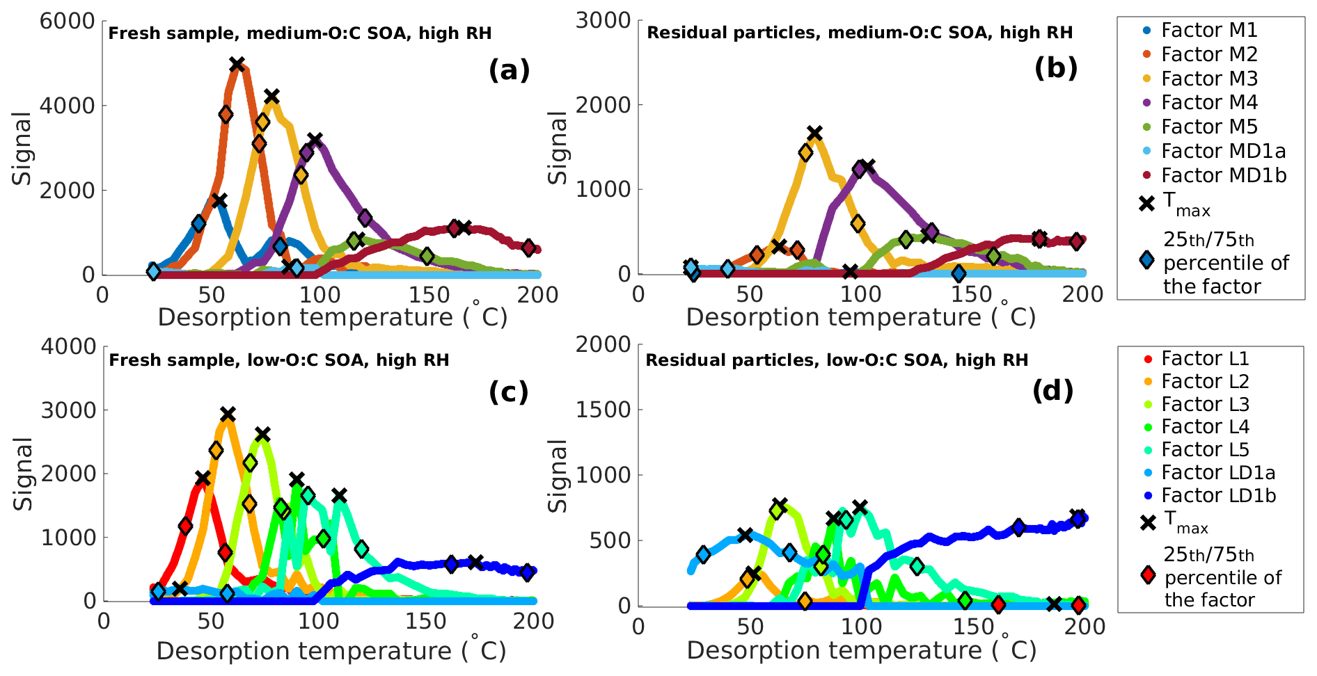
Figure 1 Main positive matrix factorization (PMF) mass loading profiles for the thermal desorption of secondary organic aerosol (SOA) from α-pinene at high relative humidity (RH) conditions. (a) Fresh sample of medium-O:C SOA. (b) Residual particles of medium-O:C SOA after 173–259 min of evaporation in a residence time chamber (RTC; the RTC sample). (c) Fresh sample of low-O:C SOA. (d) Residual particles of low-O:C SOA after 168–254 min of evaporation in the RTC (the RTC sample). Black crosses indicate the peak desorption temperature T_max, and the diamonds mark the 25th and 75th percentiles of the area of each factor.

Factors 1–5 in both O:C cases exhibit a monomodal peak shape and can thus be characterized by their T_max values. Factor MD1 in the medium-O:C case and factor LD1 in the low-O:C case need to be investigated more closely, as their factor mass spectrum and the sometimes bimodal mass loading profile suggest that these factors contain compounds stemming from both direct desorption (desorption T < 100 ^∘C) and thermal decomposition (desorption T > 100 ^∘C; see Buchholz et al., 2020, for details). To account for this, the factor is split into two, with the first half containing the signal from desorption temperatures below 100 ^∘C (factor M/LD1a) and the second half containing temperatures above 100 ^∘C (factor M/LD1b). We treat these factors separately. We note that now the latter half of the split factor is dominated by thermal decomposition products, so the apparent desorption temperature is actually the temperature at which thermal decomposition leads to products which desorb at this temperature. This apparent desorption temperature is thus a lower limit for the decomposing parent compound, i.e., the true volatility of these parent compounds is even lower. However, the desorption temperatures are so high that they lead to log₁₀ (C^∗) < −3 and are thus below the comparable range for VD_evap. Figure 1 (high-RH data) and Fig. S10 in the Supplement (dry-condition data) show the mass loading profiles derived from FIGAERO–CIMS measurements of medium- and low-O:C particles after we excluded the contamination and background factors and split the decomposition factors.

3.2 Volatility distribution comparison at high RH based on factor T_max

To compare VD_evap and VD_PMF, we need to determine the time interval in the evapogram that the VD_PMF represents. We collected the fresh samples directly after the size selection. As the particles were collected for 30 min, the collected sample represents particles that have evaporated from 0 up to 30 min in the organic vapor-free air. We note that this is different from the standard FIGAERO–CIMS sample collection in which the particles are collected in a quasi-equilibrium with the surrounding gas phase, and no significant evaporation occurs (Lopez-Hilfiker et al., 2014). For RTC samples, we also need to consider that not all particles have evaporated for the same time due to the filling of the RTC for ca. 20 min. We determined the minimum time the particles have evaporated in the RTC as the time when we started the sample collection minus the RTC filling time. We determined the maximum evaporation time in the RTC to be the time when we stopped the sample collection plus the filling time. These minimum and maximum comparison times are shown in Table S1 in the Supplement, and they are referred to as minimum and maximum (sample) evaporation time. The mean (sample) evaporation time is defined as being at the middle of the sample collection interval. For simplicity, we will show, in the main text, the results from the analysis in which the FIGAERO–CIMS samples were assumed to represents the particles at the mean sample evaporation time. We show the analysis in which the samples were assumed to represent the particles at minimum and maximum evaporation time in the Supplement. The choice of sample evaporation time does not affect the conclusions we draw about the analysis presented in this section.

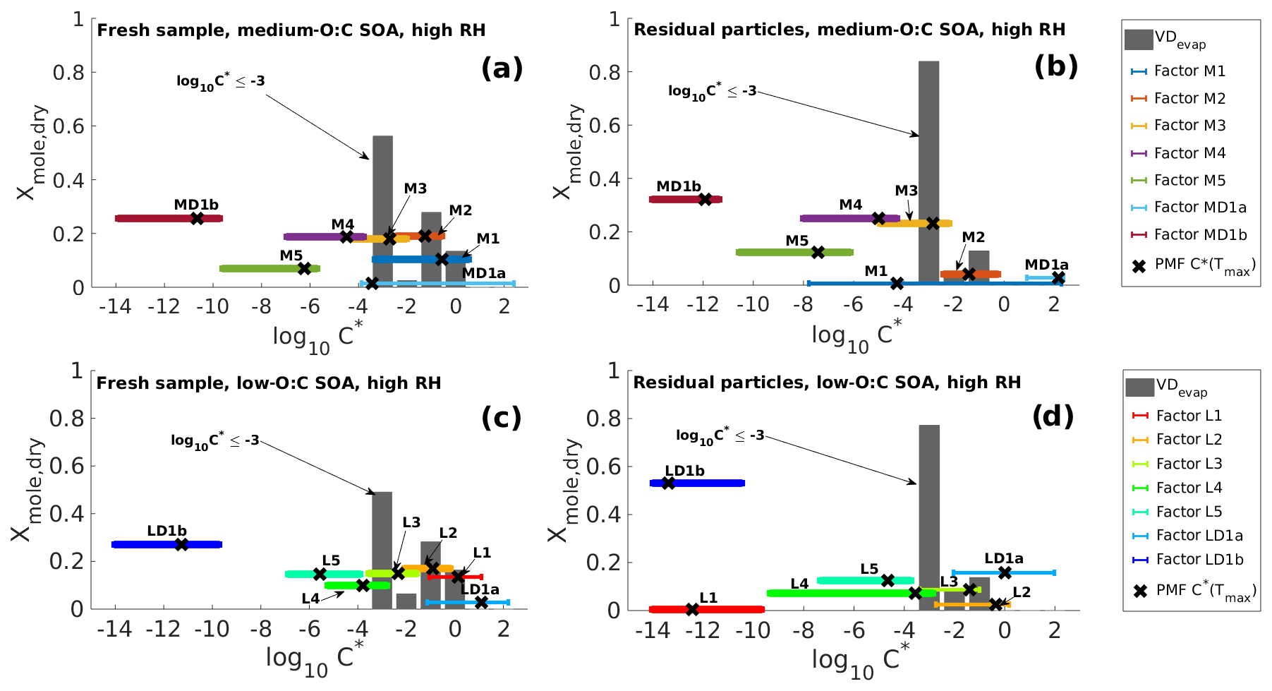
Figure 2 Volatility distributions in high-RH experiments determined from model fitting (VD_evap) and PMF analysis of FIGAERO–CIMS data (VD_PMF) for the same four cases as shown in Fig. 1. (a) Fresh sample of medium-O:C SOA. (b) Residual particles of medium-O:C SOA (the RTC sample). (c) Fresh sample of low-O:C SOA. (d) Residual particles of low-O:C SOA (the RTC sample). VD_evap is shown for the best-fit simulation (gray bars) at the mean evaporation time of the FIGAERO–CIMS sample. Black crosses show the log₁₀ (C^∗) calculated for each PMF factor from the peak desorption temperature T_max. The horizontal colored lines show the range of log₁₀ (C^∗) calculated from the 25th and 75th percentiles of each PMF factor's mass loading profile.

Figure 2 shows VD_evap and VD_PMF for medium- (Fig. 2a–b) and low-O:C (Fig. 2c–d) particles in high-RH experiments. In the VD_PMF calculated from the T_max value of each factor (black crosses), the factors fall into three different volatility classes within our chosen particle size and experimental timescale, namely practically nonvolatile (log₁₀ (C^∗) ≤ −2), slightly volatile (−2 < log₁₀ (C^∗) ≤ 0) and volatile (log₁₀ (C^∗) > 0). We use these three volatility classes to compare the volatility distributions in Fig. 3 where each VD bin is grouped to these three volatility classes. Figure 3 compares VD_PMF to what VD_evap is at the mean time that the FIGAERO samples had evaporated prior to collection. We show the same comparison for the minimum and maximum evaporation time in Fig. S6 in the Supplement.

After the volatility class grouping is applied, we see that there are differences between VD_evap and VD_PMF. With VD_PMF of the fresh samples, there are excess amounts of matter in the lowest volatility class (volatility class 1) and less material in volatility class 2 compared to VD_evap for both oxidation conditions. In addition, the VD_PMF of the low-O:C fresh sample shows more material in the highest volatility class (volatility class 3) compared to VD_evap.

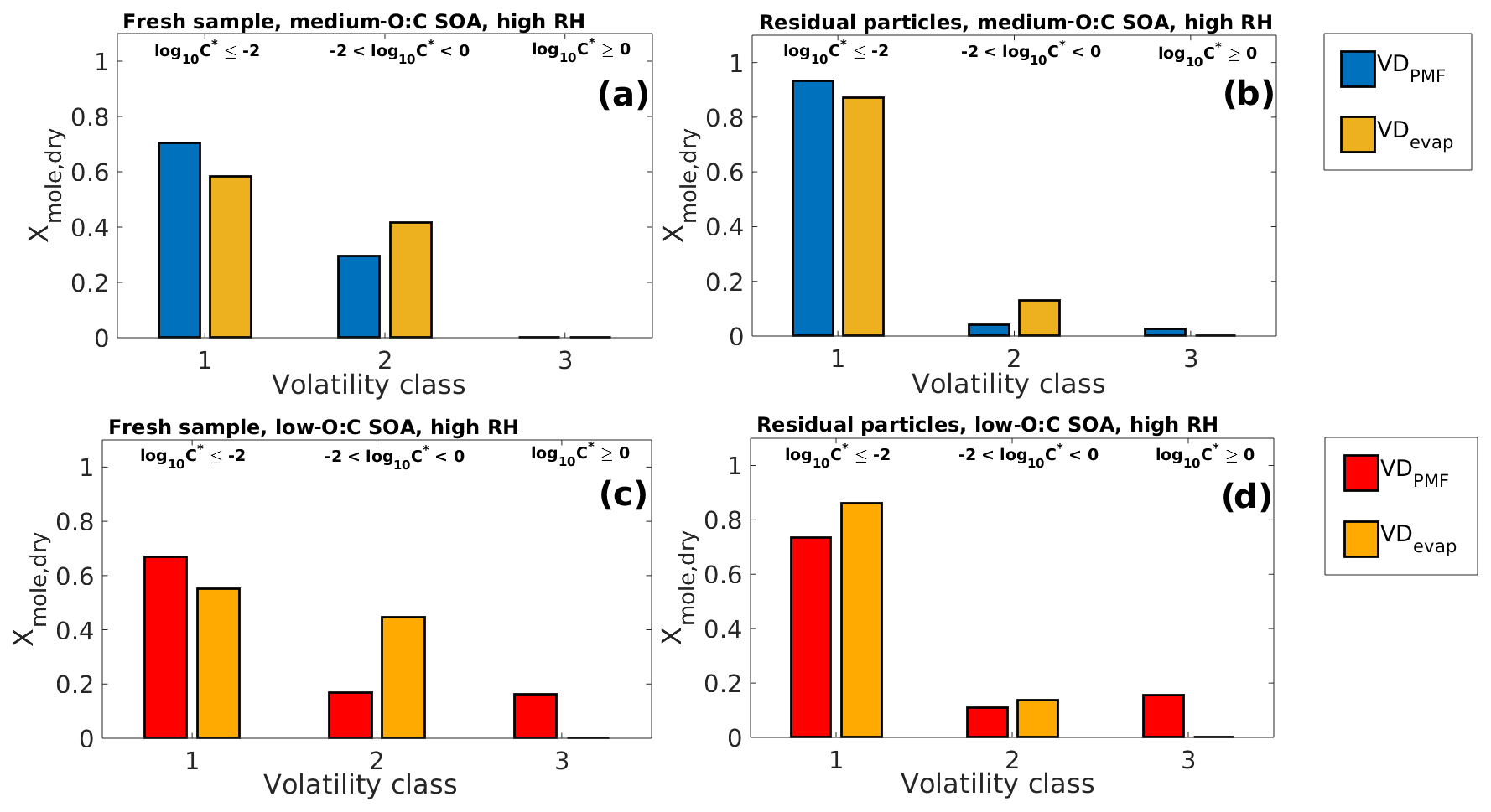
Figure 3 Comparison of VD_PMF and VD_evap at the mean sample evaporation time in high-RH experiments for the same four cases as shown in Fig. 1. (a) Fresh sample of medium-O:C SOA. (b) Residual particles of medium-O:C SOA (the RTC sample). (c) Fresh sample of low-O:C SOA. (d) Residual particles of low-O:C SOA (the RTC sample). The VD bins shown in Fig. 2 are grouped into three different volatility classes based on their evaporation tendency with respect to the measurement timescale and particle size. The limits for each volatility class are shown at the top and are the same for each subfigure. The VD_PMF shows lower overall volatility than the VD_evap, except for (d) (RTC sample of low-O:C SOA) where the VD_PMF shows higher overall volatility than the VD_evap.

Figure 4 Evapograms of high-RH experiments showing the evaporation factors (remaining fraction of the initial particle diameter; circles) and their uncertainty in time for (a) medium-O:C SOA and (b) low-O:C SOA. Liquid-like evaporation model (LLEVAP) simulated evapograms calculated using the best fit VD_evap (solid black lines) and LLEVAP simulated evapograms calculated with VD_PMF (turquoise lines for VD_PMF of fresh SOA and light brown lines for simulations with VD_PMF of the residual particles evaporated for 173–259 and 168–254 min for medium- and low-O:C SOAs, respectively). The evapograms calculated with the VD_PMF of the fresh samples show a lower rate of evaporation than the evapogram calculated with the VD_evap, which is consistent with volatility distribution shown in Fig. 3. The evapograms calculated with the VD_PMF of the residual particles (the RTC sample) show a similar rate of evaporation for medium-O:C SOA and a faster rate of evaporation for low-O:C SOA compared to evapograms calculated with VD_evap, which is similarly consistent with Fig. 3.

To investigate the observed discrepancies further, we used the VD_PMF shown in Fig. 2 as an input to the LLEVAP model and calculated the corresponding isothermal evaporation behavior (i.e., the evapogram). We show these simulated evapograms in Fig. 4a for the medium-O:C case and in Fig. 4b for the low-O:C condition together with the simulated evapogram calculated using VD_evap as an input for the LLEVAP model. The simulated evapograms calculated with the VD_PMF of the fresh samples do not match the measured evapograms, while the evapogram calculated with VD_evap agrees well with the experimental evapogram (black lines in Fig. 4), as expected, since this is the goal of the VD_evap determination. The simulation calculated with the VD_PMF of the fresh sample (light blue lines in Fig. 4 for the mean evaporation time; Fig. S7 in the Supplement for other evaporation times) shows slower evaporation than the observations or the simulation calculated with VD_evap. This is consistent with the results show in Fig. 3, where the VD_PMF contained more low-volatility material than the VD_evap.

Figure 4 also shows the simulated evapograms calculated with VD_PMF of the RTC samples (light brown lines in Figs. 4 and S7). In these cases, the particles size decreases little within the simulation timescale. With medium-O:C particles, the simulated evaporation matches the measured evaporation well. With low-O:C particles, the evaporation calculated with VD_PMF is too fast. The shape of the evapogram does not match the measured one.

3.3 Applying desorption range to characterize the volatility of PMF factors

The T_max value is a practical choice for the characteristic temperature of the desorption process. However, as we saw in Sect. 3.2, the VD_PMF calculated from the peak desorption temperatures did not produce the measured evapogram when used as an input for the LLEVAP model. Working under the assumption that all material collected on the FIGAERO filter, including the higher volatility material, is detected in the CIMS and then captured in the PMF analysis, we will relax the assumption that the volatility of the factor is characterized strictly by the T_max value of the factor and investigate the VD_PMF further. We will explore how the VD_PMF changes when the desorption temperature and the resulting C^∗ are interpreted to contain uncertainty and if the VD_PMF, considering these uncertainty ranges, is consistent with the observed isothermal evaporation. The uncertainty in the desorption temperature raises from the fact that compounds volatilize from the FIGAERO filter throughout the heating, and therefore, one value might not be adequate to characterize the C^∗ of a factor and each PMF factor contains multiple compounds with distinct C^∗.

Table 2 The best-fit C^∗ values for medium- and low-O:C high-RH experiments, when C^∗ values of PMF factors were optimized with respect to the measured isothermal evaporation. C^∗ values were optimized by assuming that the FIGAERO–CIMS sample represents particle composition at the mean sample evaporation time for the fresh sample and the minimum sample evaporation time for the RTC sample. The C^∗ values are rounded to two significant digits and are in units µg m⁻³. C^∗ values below 10⁻³ µg m⁻³ are not reported explicitly since the evapogram-fitting method is not sensitive to these values.

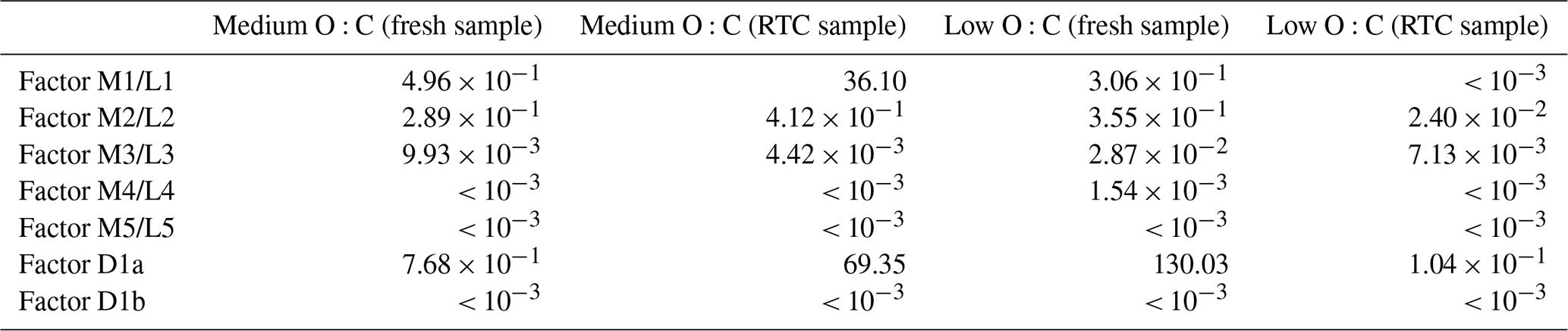
We calculated the 25th and 75th percentiles of the desorption temperatures of each factor and converted them to effective saturation concentrations, as described in Sect. 2.4 (see diamond markers in Fig. 1). We show the resulting C^∗ ranges in Fig. 2 as solid horizontal lines, where the line color matches the color of the factors in Fig. 1. We then ran the MCGA optimization by setting the number of compounds equal to the number of PMF factors, the molar fraction for each compound at the FIGAERO–CIMS sampling time fixed to the molar fraction of the corresponding factor and the C^∗ as the optimized variables restricted to the range corresponding to the 25th and 75th percentile desorption temperature. In the optimization, the goodness-of-fit statistic was calculated as a mean squared error, similar to the determination of VD_evap.

As the fresh samples were collected between 0 and 30 min from the start of the evaporation, we sought a fitting set of C^∗ values for evaporation starting at 0, 15 and 30 min. Again, we show the results for the mean sample evaporation time (15 min) in the main text and the results for the other evaporation times in the Supplement. Due to scarcity of particle size measurements at the collection time of the RTC sample, we will apply this analysis only to the VD_PMF of the RTC sample at its minimum evaporation time. In each optimization, we set the initial particle diameter to be the same as what is simulated with VD_evap. We derived 50 C^∗ estimates for both samples. From these 50 estimates, we chose the best-fit evapogram. We refer to these optimized volatility distributions as VD_PMF,opt to separate them from the VD_PMF where we used T_max to characterize C^∗ of a PMF factor.

We show the optimized C^∗ values forming VD_PMF,opt in Table 2 (see Table S2 in the Supplement for results with minimum and maximum sample evaporation times). Figure 5 shows the best-fit evaporation simulations calculated with VD_PMF,opt. The other sample evaporation times are displayed in the Supplement (Fig. S8). For both oxidation conditions, the simulations resemble the experimental evapogram and the evapogram calculated with VD_evap, although the simulation of the medium-O:C condition shows a 5 times larger goodness-of-fit value compared to the simulation calculated with VD_evap. The evapograms determined with the VD_PMF,opt of the RTC samples agree with the measured evaporation as well.

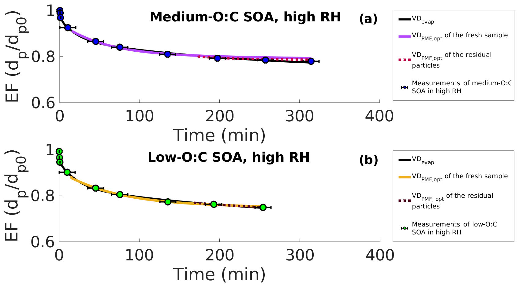
Figure 5 Evapograms of high-RH experiments showing the evaporation factors (circles), their uncertainty in time (black whiskers), the best-fit simulated evapogram calculated with VD_evap (solid black line) and the best-fit simulated evapograms calculated with the volatility distribution, where the effective saturation concentration (C^∗) of each of the PMF factors is fitted to the measurements (VD_PMF,opt). (a) Medium-O:C SOA. (b) Low-O:C SOA. The solid colored lines are for the fresh SOA, and the dashed lines are for the residual particles collected from the RTC after 173–259 and 168–254 min of evaporation for medium- and low-O:C SOAs, respectively. For fitting, the C^∗ of each PMF factor was allowed values from their respective 25th and 75th percentile desorption temperatures, as shown in Fig. 1. All the evapograms calculated with the VD_PMF,opt match the measured evaporation, highlighting that the volatility distribution determined from the FIGAERO–CIMS data with the PMF method can describe the dynamics of evaporating SOA particles when uncertainties in the C^∗ of the factors are considered.

Overall, the results demonstrate that the information derived from the fresh and RTC FIGAERO–CIMS samples can describe the volatility of the evaporating particles when uncertainties in the desorption temperature are considered.

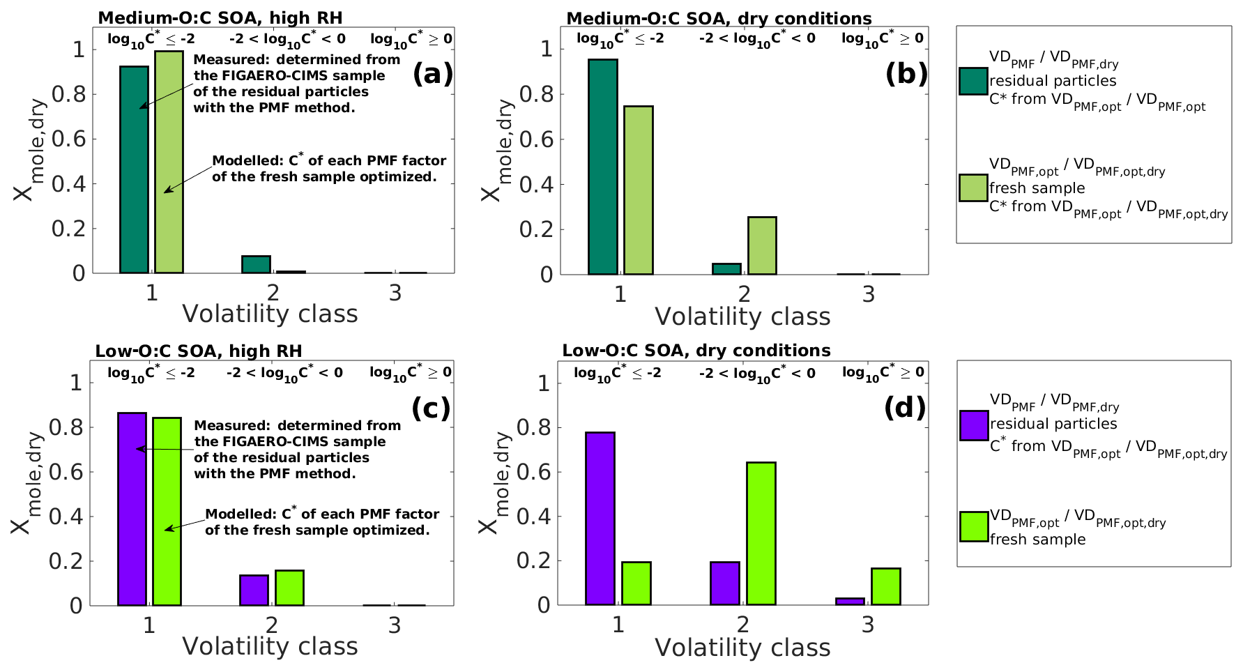
Figure 6 Comparison of the simulated particle composition (VD_PMF,opt; ${\mathrm{VD}}_{\mathrm{PMF},\mathrm{opt},\mathrm{dry}}$) to the particle composition determined from the residual particles collected from the RTC (VD_PMF/VD_PMF,dry) after 173–259 and 168–254 min of evaporation for medium- and low-O:C SOAs, respectively. The comparison is done at the mean evaporation time of the residual particles. The simulated compositions (VD_PMF,opt – a and c; ${\mathrm{VD}}_{\mathrm{PMF},\mathrm{opt},\mathrm{dry}}$ – b and d) are taken from the best-fit simulated evapogram obtained from the optimization of the C^∗ values of the fresh sample's PMF factors to the measured evapogram. The volatility of the individual volatility distribution (VD) bins are grouped into three volatility classes, similar to Fig. 3. The limits for each volatility class are shown at the top and are the same for each subfigure. The C^∗ values from VD_PMF,opt/${\mathrm{VD}}_{\mathrm{PMF},\mathrm{opt},\mathrm{dry}}$ were used for corresponding VD_PMF/VD_PMF,dry when the volatility grouping was calculated in order to ensure the comparability. (a) Medium-O:C SOA in the high-RH experiment. (b) Medium-O:C SOA in the dry-condition experiment. (c) Low-O:C SOA in the high-RH experiment. (d) Low-O:C SOA in the dry-condition experiment. In the high-RH cases (a) and (c), the volatility distributions simulated, based on VD_PMF,opt of the fresh SOAs, are similar to the measured VD_PMF, while for the dry-condition cases (b) and (d), the volatility distributions simulated, based on ${\mathrm{VD}}_{\mathrm{PMF},\mathrm{opt},\mathrm{dry}}$, show higher volatility than the measured VD_PMF.

3.4 Comparison of the volatility distribution of the fresh and RTC sample in high-RH conditions

In this section, we compare VD_PMF,opt of the fresh samples to VD_PMF of the RTC sample to study if the two VD are similar. We compare the two VD at the mean evaporation time of the RTC sample. We calculated the evapograms with the VD_PMF,opt of the fresh sample as the initial particle composition and recorded the mole fraction of each factor at the mean evaporation time of the RTC sample (216 min for medium-O:C particles and 211 min for low-O:C particles). Figure 6a and c show this comparison for both medium- and low-O:C particles. The factors are grouped into the three volatility classes described in Sect. 3.2. In Fig. 6, we show the results from the analysis where VD_PMF,opt was optimized by assigning the fresh sample composition at the mean sample evaporation time. Similar comparisons using the minimum and maximum evaporation time of the fresh sample are shown in Fig. S9 in the Supplement. To ensure that the factors are grouped to the same volatility classes for each studied VD, we used the C^∗ values of the VD_PMF,opt at the mean sample evaporation time as a basis for the grouping.

The compositions simulated, based on the VD_PMF,opt of the fresh samples, are comparable to the corresponding VD_PMF of the RTC sample in both oxidation conditions (Fig. 6). The agreement is good, especially for the low-O:C case for which the VD_PMF,opt showed a slightly smaller contribution in volatility class 1 and a corresponding higher contribution in volatility class 2 compared to the VD_PMF of the RTC sample (Fig. 6c). For the medium-O:C case, the VD_PMF,opt predicted a higher contribution of volatility class 1 and a lower contribution of volatility class 2 compared to VD_PMF (Fig. 6a).

These results show that the particle composition measured after a few hours of evaporation is consistent with the composition predicted, based on the composition observed at the start of evaporation, while considering the uncertainties of the interpreted C^∗ values.

3.5 Volatility distribution comparison in dry conditions

Next, we analyzed the evaporation experiments in dry conditions where the evaporation rate was reduced compared to the high-RH conditions. We interpreted this difference as an indication of particle-phase diffusion limitations in dry conditions (Yli-Juuti et al., 2017). Using the initial particle composition information obtained from the high-RH experiments and the FIGAERO–CIMS data, we explored the effect of particle viscosity on the evaporation process. Our aim is to test if the slower evaporation, presumably due to higher viscosity of the SOAs, can be captured with a recently developed viscosity parametrization based on glass transition temperatures of various organic compounds (DeRieux et al., 2018). We also compare the results, using the viscosity parametrization, to an approach where we fit both the viscosity and VD to the evapogram.

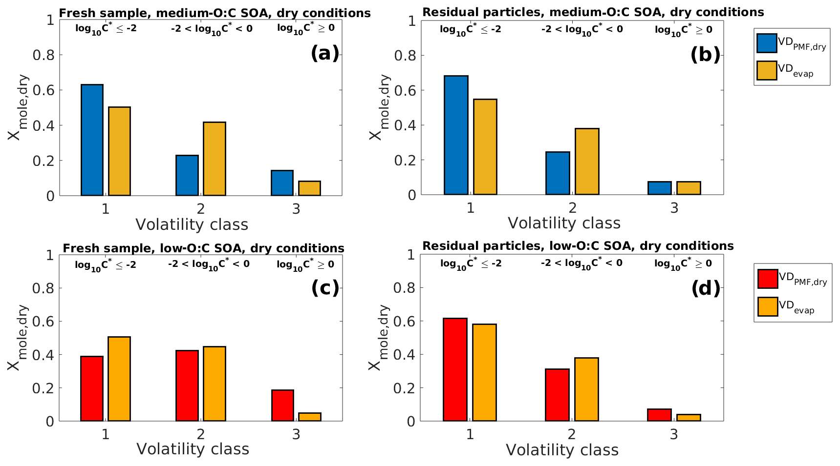
Figure 7 Comparison of VD_PMF,dry (volatility distribution with C^∗ calculated from the peak desorption temperature, T_max, of each PMF factor) and VD_evap (volatility distribution determined by fitting the LLEVAP model to the measured evapogram) at the mean evaporation time of the SOA samples in dry-condition experiments. The VD bins are grouped into three volatility classes, similar to Fig. 3. The limits for each volatility class are shown at the top and are the same for each subfigure. (a) Fresh sample of medium-O:C SOA. (b) Residual particles of medium-O:C SOA after 170–256 min of evaporation (the RTC sample). (c) Fresh sample of low-O:C SOA. (d) Residual particles of low-O:C SOA after 152–238 min of evaporation (the RTC sample). The VD_PMF,dry shows lower overall volatility than the VD_evap for medium-O:C SOA. For low-O:C SOA, the VD_PMF,dry shows higher volatility for the fresh sample and similar volatility compared to the VD_evap after 152–238 min of evaporation.

First, we investigated the range of particle viscosities that are required to explain the observed slower evaporation in dry conditions. For this, we simulated the particle evaporation in dry conditions based only on the evapogram data. We used the VD_evap (i.e., the initial particle composition obtained by optimizing mole fractions of VD bins with respect to the observed evapogram in high-RH conditions) as the initial particle composition estimate for the simulations and optimized the b_i values (Eq. 3) for each VD bin. The best-fit simulation from this optimization agrees well with the observed size decrease in the dry experiments for both low- and medium-O:C particles (Fig. 8; black line). Based on these simulations, the viscosity of the particles needs to increase from below 10⁵ Pa s to approximately 10⁸ Pa s during the evaporation in order to explain the evaporation rate observed for the dry particles.

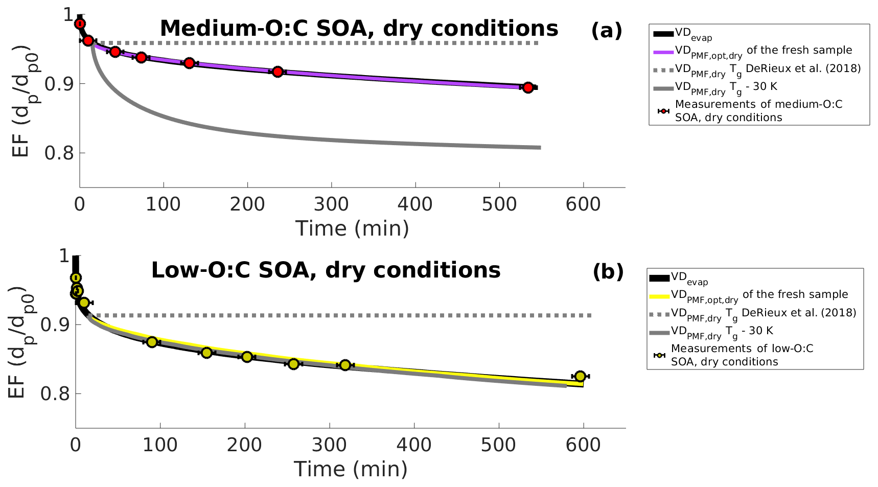
Figure 8 Evapograms showing the measured isothermal evaporation of (a) medium-O:C SOA and (b) low-O:C SOA in dry-condition experiments (markers and black whiskers) together with the simulated evapograms. The best-fit simulated evapogram calculated with VD_evap (obtained from high-RH experiments) and optimizing b_i is shown with a solid black line. Gray lines show the minimum and maximum possible evaporation calculated, with the VD_PMF,dry (C^∗ of PMF factors calculated from T_max) at the highest (the original parametrization of DeRieux et al., 2018; dashed gray lines) or the lowest (30 K subtracted from the T_g of every ion; solid gray line) studied viscosity. Solid purple and yellow lines show the best-fit simulated evapograms calculated with the optimized ${\mathrm{VD}}_{\mathrm{PMF},\mathrm{opt},\mathrm{dry}}$ (based on the assumption that the FIGAERO sample represents particles at the mean of the sample collection interval) and b_i restricted (based on the DeRieux et al., 2018, parameterization). The figure shows, similar to Fig. 5, that the volatility distribution determined from the FIGAERO–CIMS data with the PMF method is consistent with the measured evaporation of the SOA particles once the uncertainty in the effective saturation concentration and the glass transition temperature parametrization of DeRieux et al. (2018) are considered.

Second, we tested the performance of the composition-dependent viscosity parameterization by DeRiuex et al. (2018) together with the PMF results. For this, we calculated the volatility distribution, VD_PMF,dry, based on the T_max values of the factors from the fresh sample of the evaporation experiment at dry conditions (in the same way as for VD_PMF for the high-RH case). The mole fraction of each factor was calculated from the mass loading profile to give the initial mole fraction of each VD bin for the simulations. We assigned this VD_PMF,dry as the particle composition at the mean evaporation time of the fresh sample, i.e., 15 min, and simulated the particle evaporation from there onwards. The particle size at the beginning of the simulation (i.e., at 15 min of evaporation) was taken from the above simulations and optimized based only on the evapogram data, which fitted well to the measurements. We calculated the viscosity parameter b_i value for each VD bin, as described in Sect. 2.5, based on the mass spectra of the factor and the parameterization by DeRieux et al. (2018). In practice, this resulted in too high a viscosity for the particles to evaporate at all during the length of the experiment for both low- and medium-O:C particles (dashed gray line in Fig. 8). Therefore, we also conducted a simulation where the viscosity parameter b_i value for each factor was calculated based on the viscosity parameterization by setting the T_g values of all compounds 30 K lower than the parametrization predicted, which is in line with the uncertainties reported by DeRiuex et al. (2018). In this case, the simulated evaporation was faster than observed for the medium-O:C conditions (solid gray line in Fig. 8a) and similar to the evapogram calculated with the VD_evap for low-O:C conditions (solid gray line in Fig. 8b). This suggests that the observed evaporation rate at dry conditions and the viscosity parametrization by DeRieux et al. (2018) may be consistent with each other within the uncertainty range of the viscosity parametrization and the uncertainty range of the C^∗ of PMF factors.

Similar to Fig. 3, we show in Fig. 7 the comparison of VD_PMF,dry (C^∗ from T_max) to the VD_evap in dry conditions and at the mean sample evaporation time, with the VD bins grouped into the three volatility classes. We show the mass loading profiles and the volatility distributions of the experiments in dry conditions in Figs. S10 and S11 in the Supplement. Figure S12 in the Supplement shows the same comparison as Fig. 7 for other sample evaporation times. For medium-O:C particles, VD_PMF,dry calculated from the fresh sample has more contributions from volatility classes 1 and 3 and less from volatility class 2, compared to the corresponding VD_evap. For the low-O:C particles, the VD_PMF,dry of the fresh sample has more contribution from volatility class 3 and less from volatility classes 1 and 2, compared to the VD_evap. For medium-O:C particles, the differences between the VD_PMF,dry and VD_evap leave open the possibility that the underestimated evaporation rate calculated using VD_PMF,dry is partly a result of inaccuracy in the volatility description and not solely due to the high estimated viscosity. For the low-O:C particles, the underestimated evaporation most likely stems from the high estimated viscosity since VD_PMF,dry is shifted towards higher volatility compounds than VD_evap.

As a third investigation of the viscosity, we again used the PMF results of the fresh sample in dry conditions to initialize the particle composition in the model at the mean fresh sample evaporation time. The mole fraction of each factor was calculated from the mass loading profile, giving the initial mole fraction of each VD bin for the simulations a similar one to the high-RH analysis. Then, using the MCGA algorithm together with the KM-GAP model, we estimated the b_i coefficient and C^∗ of each VD bin by optimizing the KM-GAP-simulated evapogram to the measured evapogram in dry conditions. This way, we obtained both the initial volatility distribution (${\mathrm{VD}}_{\mathrm{PMF},\mathrm{dry},\mathrm{opt}}$) and viscosity parameters b_i simultaneously. For this optimization, we restricted the C^∗ values of the factors based on the 25th and 75th percentile of the desorption temperature of the factors (similar to what was done above for VD_PMF,opt) and the viscosity parameter b_i values, based on the DeRieux et al. (2018) parameterization. The b_i values calculated with the original parametrization by DeRieux et al. (2018) were set as the upper limit for the b_i values. The lower limit for the b_i values was calculated by setting the glass transition temperature of each compound 30 K lower than the parametrization predicted. As above, in these simulations the initial particle size was also taken from the simulations where the optimization was based only on the evapogram data. For both medium- and low-O:C particles, it was possible to find a set of C^∗ and b_i values that produced an equally good match to the experimental data as the VD_evap (purple and yellow lines in Fig. 8).

Figure 6b and d show the comparison of the measured and simulated particle composition, grouped into the three volatility classes, at the RTC sample collection time for the dry experiments for low- and medium-O:C particles. The measured composition is the VD calculated from the PMF results of the RTC samples in dry conditions. The optimized C^∗ values of the factors from the corresponding dry experiment were used for these VD. The simulated particle composition is taken from the optimized model run (optimized ${\mathrm{VD}}_{\mathrm{PMF},\mathrm{opt},\mathrm{dry}}$ and b_i) at the mean RTC sample collection time, similar to the high-RH cases presented in Fig. 6a and c. For low-O:C particles, there is a clear discrepancy as the ${\mathrm{VD}}_{\mathrm{PMF},\mathrm{dry},\mathrm{opt}}$ implies a much larger relative contribution from volatility classes 2 and 3 and a smaller contribution from volatility class 1 when compared to the measurements. This inconsistency may be related to the rather high viscosities in the simulations. The viscosity of the low-O:C particles in this optimized simulation was rather high, at η > 10⁸ Pa s throughout the evaporation, slowing the evaporation of the higher volatility compounds. A similar evaporation curve could be obtained with lower viscosity and lower volatilities of the VD bins.

4 Discussion

Qualitatively, VD_PMF and VD_PMF,dry capture the evaporation dynamics well in all studied cases; quantitatively, there were discrepancies. For the VD_PMF of the fresh samples, the first and second factor desorb at low heating temperatures (below 100 ^∘C), indicating that these factors represent high-volatility organic compounds that evaporate almost completely from the particles in the experimental timescale of our isothermal evaporation experiments. In the RTC samples, these factors show significantly lower or nonexisting signal strength relative to the other factors. The factors that desorb at high temperatures show an increase in the relative signal strength in the RTC samples compared to the fresh samples, which is consistent with the expected increase in the relative contribution of lower volatility compounds along evaporation. These findings indicate that the FIGAERO–CIMS measurements of α-pinene SOAs and the applied PMF method give a good overall picture of the evolution of the volatility distribution during evaporation.

In addition to the PMF method used here, other ways of characterizing SOA compound volatilities or VBS from FIGAERO–CIMS thermograms have also been suggested (e.g., Stark et al., 2017). These include, for example, the more straightforward method of calculating the C^∗ of each detected ion based on their T_max, using Eq. (3) and lumping them into a traditional VBS. While such other methods may capture the volatility distributions sufficiently, the benefit of PMF method is that it offers a new way to understand what happens inside the particles, e.g., during the heating in FIGAERO. Here we have evaluated this method with respect to its ability to capture the volatilities of SOAs.

At high RH, the VD_PMF that was derived from the T_max of each factor's mass loading profile did not produce an evapogram similar to the measured ones when the VD_PMF was used as an input for the LLEVAP model. This reflects the sensitivity of the particle evaporation to the C^∗ values and suggests that the VD_PMF is not directly applicable as a particle composition estimate for a detailed particle dynamics study. When we allowed uncertainty in the C^∗ values of each factor, we were able to explain most of the discrepancies between the simulated and measured evapograms. Our results also demonstrate the need for careful investigation of the representative time of the sample when filter-collected samples are applied for dynamic processes such as evaporation.

In this study we assumed a quite large uncertainty range for the desorption temperature of each PMF factor, and it is not certain that the determination of VD_PMF,opt would be successful if the allowed ranges for C^∗ of PMF factors were lower. Thus, work remains to be done in studying what the total uncertainty is that arises from combining the FIGAERO–CIMS measurements with the PMF method and to what extent the PMF factors can be thought to represent surrogate organic compounds for the purpose of detailed SOA dynamics studies.

We note that care has to be taken when PMF results are transferred to volatility distributions, especially with regard to separating the contribution of instrument background and contamination from the true sample. When the sample mass was low (in the low-O:C RTC sample), we noticed that the first half of the bimodal (factor LD1a) resulted in a high mole fraction even though the absolute signal strength of the factor did not change between the fresh and the RTC sample, which is usually an indication that this signal is caused by instrument background. However, the signal strength of this factor was low enough in all cases to not affect the overall VD estimation. More details on the interpretation of B- and D-type factors and potential factor blending can be found in Buchholz et al (2020).

In dry conditions, VD_PMF,dry of the fresh sample in the low-O:C case showed a noticeably higher amount of high-volatility matter than VD_evap. This discrepancy between the volatility distributions is not expected and raises a need for further studies on the role of viscosity and possible particle-phase chemistry in SOA particle dynamics. Future studies should investigate the possibility of chemical reactions that modify the volatility of organic compounds and how viscosity is described in process models.

5 Conclusions

We compared volatility distributions derived from FIGAERO–CIMS measurements with PMF analysis to volatility distributions derived from fitting a process model to match the measured size change in particles during isothermal evaporation. We compared the two methods for obtaining the volatility-distribution data for two different particle compositions and two evaporation conditions. The results are promising and suggest that the methods provide volatility distributions that are in agreement. We note that the data set available here is limited and additional investigations on comparing the methods are desirable in the future.

In all studied experimental data sets, we were able to capture the measured evaporation with the fitting method. In high-RH experiments, VD_PMF deviated from VD_evap, especially when the FIGAERO samples were collected at the early stages of the evaporation. However, qualitatively, both types of VD evolved similarly, i.e., the fraction of lower volatility compounds increased, and the fraction of higher volatility compounds decreased during the evaporation of the particles. These results suggest that the changes in FIGAERO–CIMS-derived volatility distributions over the isothermal evaporation are consistent with the observed isothermal evaporation, and the detailed SOA dynamics are sensitive to the uncertainties in the C^∗ values.

The volatility distribution derived with the PMF method at high RH agreed with the observed isothermal evaporation better when we interpreted the volatility of each factor as a range of possible C^∗ values and optimized the C^∗ values within these ranges with respect to the measurements. These results suggest that the FIGAERO–CIMS measurements combined with PMF method not only provide qualitative information of the volatilities of the SOA constituents but they also have the potential for quantitative investigations of the volatility distributions. However, more work is needed to constrain the uncertainties rising from the conversion of the FIGAERO–CIMS desorption temperatures to C^∗ values, and it should be noted that deriving the volatilities based on only the T_max of PMF factors may not be sufficient for representing detailed SOA dynamics.

In dry conditions, we were able to simulate the evapograms based on the PMF results, using the VTF equation and the glass transition temperature parametrization of DeRieux et al. (2018), if both C^∗ and viscosity parameters were optimized and allowed to contain reasonable uncertainties. For both oxidation conditions, the measured composition at the later stages of the evaporation suggested considerably lower volatility than the simulations. These results suggest that the tested viscosity parameterization is not in disagreement with the observed SOA evaporation; however, the uncertainties related to the method are significant from the point of view of simulating SOA dynamics.

Based on our analysis, we conclude that using the PMF method with FIGAERO–CIMS thermogram data is good for estimating the volatility distribution of organic aerosols when the organic compounds present in the particle phase have low volatilities with respect to the sample collection and analysis timescale. Specifically, VD_PMF is useful for extracting information about organic compounds that do not evaporate during the evaporation measurements at room temperature. VD_PMF is applicable for detailed particle dynamics studies when the desorption temperature of the factor is characterized with a range around the T_max value. Furthermore, combining VD_PMF,opt with detailed process modeling and input optimization could allow the quantification of other physical or chemical properties of organic aerosols since the FIGAERO–CIMS data constrain the particle composition and effectively decrease the search space that needs to be explored with global optimization methods.