the Creative Commons Attribution 4.0 License.
the Creative Commons Attribution 4.0 License.
 | 08 Sep 2020
Characterizing sources of high surface ozone events in the southwestern US with intensive field measurements and two global models
Meiyun Lin
Andrew O. Langford
Larry W. Horowitz
Christoph J. Senff
Elizabeth Klovenski
Yuxuan Wang
Raul J. Alvarez II
Irina Petropavlovskikh
Patrick Cullis
Chance W. Sterling
Jeff Peischl
Thomas B. Ryerson
Steven S. Brown
Zachary C. J. Decker
Guillaume Kirgis
Stephen Conley
The detection and attribution of high background ozone (O3) events in the southwestern US is challenging but relevant to the effective implementation of the lowered National Ambient Air Quality Standard (NAAQS; 70 ppbv). Here we leverage intensive field measurements from the Fires, Asian, and Stratospheric Transport−Las Vegas Ozone Study (FAST-LVOS) in May–June 2017, alongside high-resolution simulations with two global models (GFDL-AM4 and GEOS-Chem), to study the sources of O3 during high-O3 events. We show possible stratospheric influence on 4 out of the 10 events with daily maximum 8 h average (MDA8) surface O3 above 65 ppbv in the greater Las Vegas region. While O3 produced from regional anthropogenic emissions dominates pollution events in the Las Vegas Valley, stratospheric intrusions can mix with regional pollution to push surface O3 above 70 ppbv. GFDL-AM4 captures the key characteristics of deep stratospheric intrusions consistent with ozonesondes, lidar profiles, and co-located measurements of O3, CO, and water vapor at Angel Peak, whereas GEOS-Chem has difficulty simulating the observed features and underestimates observed O3 by ∼20 ppbv at the surface. On days when observed MDA8 O3 exceeds 65 ppbv and the AM4 stratospheric ozone tracer shows 20–40 ppbv enhancements, GEOS-Chem simulates ∼15 ppbv lower US background O3 than GFDL-AM4. The two models also differ substantially during a wildfire event, with GEOS-Chem estimating ∼15 ppbv greater O3, in better agreement with lidar observations. At the surface, the two models bracket the observed MDA8 O3 values during the wildfire event. Both models capture the large-scale transport of Asian pollution, but neither resolves some fine-scale pollution plumes, as evidenced by aerosol backscatter, aircraft, and satellite measurements. US background O3 estimates from the two models differ by 5 ppbv on average (greater in GFDL-AM4) and up to 15 ppbv episodically. Uncertainties remain in the quantitative attribution of each event. Nevertheless, our multi-model approach tied closely to observational analysis yields some process insights, suggesting that elevated background O3 may pose challenges to achieving a potentially lower NAAQS level (e.g., 65 ppbv) in the southwestern US.
- Article
(19101 KB) - Full-text XML
- Companion paper
-
Supplement
(1998 KB) - BibTeX
- EndNote


Surface ozone (O3) typically peaks over the high-elevation southwestern US (SWUS) in late spring, in contrast to the summer maximum produced from regional anthropogenic emissions in the low-elevation eastern US (EUS). The springtime O3 peak in the SWUS partly reflects the substantial influence of background O3 from natural sources (e.g., stratospheric intrusions) and intercontinental pollution (Zhang et al., 2008; Fiore et al., 2014; Jaffe et al., 2018). These “non-controllable” O3 sources can episodically push surface daily maximum 8 h average (MDA8) O3 to exceed the National Ambient Air Quality Standard (NAAQS; Lin et al., 2012a, 2012b; Langford et al., 2017). Identifying and quantifying the sources of springtime high-O3 events in the SWUS has been extremely challenging owing to limited measurements, complex topography, and various O3 sources (Langford et al., 2015). As the O3 NAAQS becomes more stringent (lowered from 75 to 70 ppbv since 2015), quantitative understanding of background O3 sources is of great importance for screening exceptional events, i.e., “unusual or naturally occurring events that can affect air quality but are not reasonably controllable using techniques that tribal, state or local air agencies may implement” (U.S. Environmental Protection Agency, 2016). Here we leverage intensive measurements from the 2017 Fires, Asian, and Stratospheric Transport-Las Vegas Ozone Study (FAST-LVOS; Langford et al., 2020), alongside high-resolution simulations with two global atmospheric chemistry models (GFDL-AM4 and GEOS-Chem), to characterize the sources of high-O3 events in the region. Through a process-oriented analysis, we aim to understand the similarities and disparities between these two widely used global models in simulating O3 in the SWUS.
Mounting evidence shows that a variety of sources contribute to the high surface O3 found in the SWUS during spring. For example, observational and modeling studies show that deep stratospheric intrusions can episodically increase springtime MDA8 O3 levels at high-elevation SWUS sites by 20–40 ppbv (Langford et al., 2009; Lin et al., 2012a). Large-scale transport of Asian pollution across the North Pacific also peaks in spring due to active midlatitude cyclones and strong westerly winds, contributing to some high-O3 events and raising mean background O3 levels over the SWUS (Jacob et al., 1999; Lin et al., 2012b, 2015b, 2017; Langford et al., 2017). Moreover, frequent wildfires complicate the study of O3 in the SWUS (Jaffe et al., 2013, 2018; Baylon et al., 2016; Lin et al., 2017). In the late spring and early summer, increased photochemical activity from US domestic anthropogenic emissions can prevent the unambiguous attribution of observed high-O3 events in this region to background influence.
Quantifying the contributions of different O3 sources relies heavily on numerical models. Previous studies, however, have shown large model discrepancies in the estimates of North American background O3 (NAB), defined as O3 that would exist in the absence of North American anthropogenic emissions. Zhang et al. (2011) applied GEOS-Chem to quantify NAB O3 during March–August of 2006–2008 and estimated a mean of 40±7 ppbv at SWUS high-elevation sites, while Lin et al. (2012a) estimated 50±11 ppbv for the late spring to early summer of 2010 with GFDL-AM3. Emery et al. (2012) estimated mean NAB O3 to be 20–45 ppbv with GEOS-Chem and 25–50 ppbv with a regional model driven by GEOS-Chem boundary conditions during spring to summer. Large inter-model differences exist not only in seasonal means but also in day-to-day variability (e.g., Fiore et al., 2014; Dolwick et al., 2015; Jaffe et al., 2018). An event-oriented multi-model comparison, tied closely to intensive field measurements, is needed to provide process insights into this model discrepancy.
Deploying targeted measurements and conducting robust model source attribution are crucial to characterize and quantify the sources of elevated springtime O3 in the SWUS (Langford et al., 2009, 2012; Lin et al., 2012a, 2012b). This is particularly true for inland areas of the SWUS, such as greater Las Vegas, where air quality monitoring sites are sparse, making it difficult to assess the robustness of model source attribution (Langford et al., 2015, 2017). Using field measurements from the Las Vegas Ozone Study (LVOS) in May–June 2013 and model simulations, Langford et al. (2017) provided an unprecedented view of the influences of stratosphere-to-troposphere transport (STT) and Asian pollution on the exceedances of surface O3 in Clark County, Nevada. This study suggests that O3 descending from the stratosphere and sometimes mingled with Asian pollution can be entrained into the convective boundary layer and episodically brought down to the ground in the Las Vegas area in spring, adding 20–40 ppbv to surface O3 and pushing MDA8 O3 above the NAAQS. However, uncertainties remain in previous analyses due to the use of relatively coarse-resolution simulations and limited measurements to connect surface O3 exceedances at high-elevation baseline sites and low-elevation regulatory sites. High-resolution simulations and more extensive observations are thus needed to further advance our understanding of springtime peak O3 episodes in the region.
In May–June 2017, the NOAA Earth System Research Laboratory Chemical Sciences Division (NOAA/ESRL CSD) carried out the FAST-LVOS follow-up study in Clark County, NV. During this campaign, a broad suite of near-continuous observations was collected by in situ chemistry sensors deployed at a mountain-top site and by state-of-the-art ozone and Doppler lidars located in the Las Vegas Valley. These daily measurements were supplemented by ozonesondes and scientific aircraft flights during four 2 to 4 d long intensive operating periods (IOPs) triggered by the appearance of upper-level troughs above the US west coast. These extensive measurements, together with high-resolution simulations from two global models (GFDL-AM4 and GEOS-Chem), provide us with a rare opportunity to pinpoint the sources of elevated springtime O3 in the SWUS. We briefly describe the FAST-LVOS field campaign and model configurations in Sect. 2. Following an overall model evaluation (Sect. 3), we present process-oriented analyses of the high-O3 events from deep stratospheric intrusions, wildfires, regional anthropogenic pollution, and the long-range transport of Asian pollution (Sect. 4). Section 5 summarizes differences between the simulated total and background O3 determined by the two models during FAST-LVOS. Finally, in Sect. 6, the implications of the study are discussed.
2.1 FAST-LVOS measurement campaign
The FAST-LVOS experiment was designed to further our understanding of the impacts of STT, wildfires, long-range transport from Asia, and regional pollution on air quality in the Las Vegas Valley. The field campaign was carried out between 17 May and 30 June 2017 in Clark County (NV), which includes the greater Las Vegas area (Fig. 1). The measurement campaign consisted of daily lidar and in situ measurements supplemented by aircraft and ozonesonde profiling during the four IOPs (23–25 May, 31 May–2 June, 10–14 June, and 28–30 June). The daily measurements included chemical composition (e.g., CO and O3) and meteorological parameters (e.g., air temperature and water vapor) recorded with high temporal resolution by instruments installed in a mobile laboratory (Wild et al., 2017) parked on the summit of Angel Peak (36.32∘ N, 115.57∘ W; 2682 m above sea level, a.s.l.), the site of the 2013 LVOS field campaign. This mountain-top site, located ∼45 km northwest of Las Vegas City (see Fig. 1), is far from anthropogenic emission sources and mostly receives free-tropospheric air at night but is frequently influenced during the day by air transported from the Las Vegas Valley through upslope flow in late spring and summer (Langford et al., 2015). The Tunable Optical Profiler for Aerosols and oZone (TOPAZ) three-wavelength mobile differential absorption lidar (DIAL) system, which was previously deployed to Angel Peak during LVOS, was relocated to North Las Vegas Airport (NLVA; Fig. 1), where it measured 8 min averaged vertical profiles of O3 and aerosol backscatter from 27.5 to ∼8 km above ground level (a.g.l.) with an effective vertical resolution (for O3) ranging from ∼10 m near the surface to ∼150 m at 500 m a.g.l. and ∼900 m at 6 km a.g.l. The aerosol backscatter profiles were retrieved at 7.5 m resolution. TOPAZ was operated daily, but not continuously, throughout the campaign. NOAA also deployed a continuously operating micro-Doppler lidar at NLVA to measure vertical velocities and relative aerosol backscatter throughout the campaign. Boundary layer heights were inferred from the micro-Doppler measurements following the method in Bonin et al. (2018).
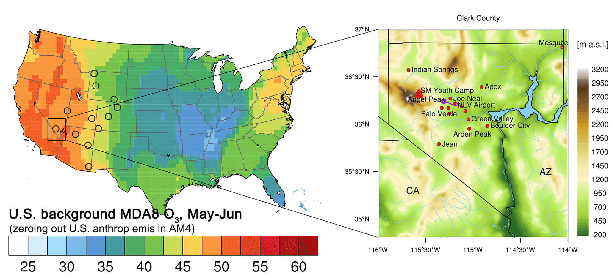
Figure 1(Left) Mean US background MDA8 O3 (ppbv) during FAST-LVOS (May–June 2017) estimated by zeroing out US anthropogenic emissions in the global high-resolution (∼50 km × 50 km) version of the GFDL-AM4 model (circles denote 12 selected high-elevation CASTNet sites); (Right) Topographic map of Clark County displaying the locations of Angel Peak (filled triangle) and regulatory O3 monitoring sites (filled circles). The purple trace denotes the Scientific Aviation flight track during 19:15–19:35 UTC of 28 June 2017. The topographic data are from NOAA's National Centers for Environmental Information (http://www.ngdc.noaa.gov/mgg/global, last access: 10 October 2019).
The routine in situ and lidar measurements described above were augmented during the four IOPs by ozonesondes launched up to four times per day (30 launches total during the entire campaign) from the Clark County Department of Air Quality Joe Neal monitoring site located ∼8 km north–northwest of the NLVA. Aircraft measurements were also conducted by Scientific Aviation to sample O3, methane (CH4), water vapor (H2O), and nitrogen dioxide (NO2) between NLVA and Big Bear, CA, during the IOPs. Readers can refer to our previous studies (Langford et al., 2010, 2015, 2017, 2019; Alvarez II et al., 2011) for detailed descriptions and configurations of TOPAZ and the other measurement instruments. The FAST-LVOS field campaign is also described in more detail elsewhere (Langford et al., 2020).
The FAST-LVOS measurements were augmented by hourly surface O3 measurements from Joe Neal and other regulatory air quality monitoring sites operated by the Clark County Department of Air Quality (Table S1 in the Supplement). Surface observations of O3 from these and other mostly urban sites were obtained from the U.S. Environmental Protection Agency (EPA) Air Quality System (AQS; https://www.epa.gov/aqs, last access: 19 March 2019). We average the AQS measurements into grids for a direct comparison with model results (as in Lin et al., 2012a, b). Surface observations from rural sites and more representative of background air were obtained from the EPA Clean Air Status and Trends Network (CASTNet; https://www.epa.gov/castnet, last access: 19 March 2019).
2.2 GFDL-AM4 and GEOS-Chem
Comparisons of key model configurations are shown in Table S2. AM4 is the new generation of the Geophysical Fluid Dynamics Laboratory chemistry–climate model contributing to the Coupled Model Intercomparison Project, Phase 6 (CMIP6). The model employed in this study, a prototype version of AM4.1 (Horowitz et al., 2020), differs from the AM4 configuration described in Zhao et al. (2018a, 2018b) by including 49 vertical levels extending up to 1 Pa (∼80 km) and interactive stratosphere–troposphere chemistry and aerosols. Major physical improvements in GFDL-AM4, compared to its predecessor GFDL-AM3 (Donner et al., 2011), include a new double-plume convection scheme with improved representation of convective scavenging of soluble tracers, new mountain drag parametrization, and the updated hydrostatic finite-volume cubed-sphere dynamical core (Zhao et al., 2016, 2018a, b). For tropospheric chemistry, GFDL-AM4 includes improved treatment of photooxidation of biogenic volatile organic compounds (VOCs), photolysis rates, heterogeneous chemistry, sulfate and nitrate chemistry, and deposition processes (Mao et al., 2013a, 2013b; Paulot et al., 2016, 2017; Li et al., 2016), as described in more detail by Schnell et al. (2018). We implement a stratospheric O3 tracer (O3Strat) in GFDL-AM4 to track O3 originating from the stratosphere. The O3Strat is defined relative to a dynamically varying e90 tropopause (Prather et al., 2011) and is subject to tropospheric chemical loss (in the same manner as odd oxygen of tropospheric origin) and deposition to the surface (Lin et al., 2012a, 2015a). The model is nudged to NCEP reanalysis winds using a height-dependent nudging technique (Lin et al., 2012b). The nudging minimizes the influences of chemistry–climate feedbacks and ensures that the large-scale meteorological conditions are similar to those observed across the sensitivity simulations. We conduct a suite of AM4 simulations at C192 ( km2) horizontal resolution for January–June 2017: (1) a base simulation (BASE) with all emissions included; (2) a sensitivity simulation without anthropogenic emissions over North America (15–90∘ N, 165–50∘ W; NAB); (3) a sensitivity simulation without anthropogenic emissions over the US (USB); (4) a sensitivity simulation without Asian anthropogenic emissions, and (5) a sensitivity simulation without wildfire emissions (see Table S3). The high-resolution BASE and sensitivity simulations for January–June 2017 are initialized from the corresponding nudged C96 ( km2) simulations spanning from 2009 to 2016 (8 years). Compared to the NAB simulation, the USB simulation includes additional contributions from Canadian and Mexican anthropogenic emissions. The USB estimates are now generically defined as “background O3” and used by the U.S. EPA. Over the western US (WUS), the vertical model resolution ranges from ∼50 to 200 m near the surface to ∼1–1.5 km near the tropopause and ∼2–3 km in much of the stratosphere.
The Goddard Earth Observing System coupled with Chemistry (GEOS-Chem; http://geos-chem.org, last access: 28 October 2019) is a widely used global chemical transport model (CTM) for simulating atmospheric composition and air quality (Bey et al., 2001; Zhang et al., 2011), driven by assimilated meteorological fields from the NASA Global Modeling and Assimilation Office (GMAO). We conduct high-resolution simulations over North America (10∘–70∘ N, 140∘–40∘ W), with 0.25∘ (latitude) ×0.3125∘ (longitude) horizontal resolution, using a one-way nested-grid version of GEOS-Chem (v11.01) (Wang et al., 2004; Chen et al., 2009) driven by the Goddard Earth Observing System – Forward Processing (GEOS-FP) assimilated meteorological data. The model uses a fully coupled NOx−OX–hydrocarbon–aerosol–bromine chemistry mechanism in the troposphere (“Tropchem”), whereas a simplified linearized chemistry mechanism (Linoz) is used in the stratosphere to simulate stratospheric ozone and cross-tropopause ozone fluxes (McLinden et al., 2000). Although GEOS-Chem can also be run with the Universal tropospheric–stratospheric Chemistry eXtension (UCX) mechanism that simulates interactive stratosphere–troposphere chemistry and aerosols (Eastham et al., 2014), this option was not used in the simulations presented in this study due to computational constraints. To further save computational resources, we used a reduced vertical resolution of 47 hybrid eta levels, by combining vertical layers above ∼80 hPa from the native 72 levels of GEOS-FP. The thickness of model vertical layers over the WUS ranges from ∼15 to 100 m near the surface to ∼1 km near the tropopause and in the lower stratosphere. Similar GEOS-Chem simulations with simplified treatments of stratospheric chemistry and dynamics have been previously used to estimate background O3 for U.S. EPA policy assessments (Zhang et al., 2011, 2014; Fiore et al., 2014; Guo et al., 2018). Thus, it is important to assess the ability of this model to represent high-background-O3 events from stratospheric intrusions. We conduct two nested high-resolution simulations with GEOS-Chem for February–June 2017: BASE and a USB simulation with anthropogenic emissions zeroed out in the US (Table S3). Initial and boundary conditions for chemical fields in the nested-grid simulations were provided by the corresponding BASE and USB GEOS-Chem global simulations at resolution for January–June 2017. Only results for April–June from the nested simulations are analyzed in this study. The 3-month spin-up period (January–March) used for GEOS-Chem is relatively short compared to the multi-year GFDL-AM4 simulations, although it should be sufficient given that the lifetime of ozone in the free troposphere is approximately 3 weeks (e.g., Young et al., 2018).
2.3 Emissions
The anthropogenic emissions used in GFDL-AM4 are modified from the CMIP6 historical emission inventory (Hoesly et al., 2018). The CMIP6 emission inventory does not capture the decreasing trend in anthropogenic NOx emissions over China after 2011 as inferred from satellite-measured tropospheric NO2 columns (Liu et al., 2016; Fig. S1 in the Supplement). We thus scale CMIP6 NOx emissions over China after 2011 based on a regional emission inventory developed by Tsinghua University (Qiang Zhang at Tsinghua University, personal communications, 13 March 2018; Fig. S1). The adjusted NOx emission trend over China agrees well with the NO2 trend derived from satellite retrievals. We also reduce NOx emissions over the EUS (25∘–50∘ N, 94.5∘–75∘ W) by 50 % following Travis et al. (2016), who suggested that excessive NOx emissions may be responsible for the common model biases in simulating O3 over the southeastern US. These emission adjustments reduce mean MDA8 O3 biases in GFDL-AM4 by ∼5 ppbv in spring and ∼10 ppbv in summer over the EUS (Fig. S2). The model applies the latest daily resolving global fire emission inventory from NCAR (FINN) (Wiedinmyer et al., 2011), vertically distributed over six ecosystem-dependent altitude layers from the ground surface to 6 km (Dentener et al., 2006; Lin et al., 2012b). Biogenic isoprene emissions (based on MEGAN; Guenther et al., 2006; Rasmussen et al., 2012), lightning NOx emissions, dimethyl sulfide, and sea salt emissions are tied to model meteorological fields (Donner et al., 2011; Naik et al., 2013).
For GEOS-Chem, anthropogenic emissions over the United States are scaled from the 2011 US NEI to reflect the conditions in 2017 (https://www.epa.gov/air-emissions-inventories/air-pollutant-emissions-trends-data, last access: 10 October 2019). Similar to AM4, we reduce EUS anthropogenic NOx emissions in GEOS-Chem by 50 % to improve simulated O3 distributions. Anthropogenic emissions over China are based on the 2010 MIX emission inventory (Li et al., 2017), with NOx emissions scaled after 2010 using the same trend as in GFDL-AM4. Biogenic VOC emissions are calculated online with MEGAN (Guenther et al., 2006). Biomass burning emissions are from the FINN inventory but implemented in the lowest model layer. The model calculates lightning NOx emissions using a monthly climatology of satellite lightning observations coupled to parameterized deep convection (Murray et al., 2012). The calculation of lightning NOx in this study differs from that in Zhang et al. (2014), who used the U.S. National Lightning Detection Network (NLDN) data to constrain model flash rates.
3.1 GFDL-AM4 versus GFDL-AM3
We first compare O3 simulations in AM4 with those from its predecessor, AM3, which has been extensively used in previous studies to estimate background O3 (Lin et al., 2012a, 2012b, 2015a; Fiore et al., 2014). Figure 2 shows the comparisons of simulated and observed March mean O3 vertical profiles and mid-tropospheric O3 seasonal cycles at the Trinidad Head and Boulder ozonesonde sites. Free-tropospheric O3 measured at both sites in March is representative of background conditions, with little influence from US anthropogenic emissions. Thus, we also show O3 from the NAB simulations with North American anthropogenic emissions zeroed out. As constrained by the availability of AM3 simulations from previous studies, we focus on the 2010–2014 period and compare the NAB estimates as opposed to the USB estimates used in the rest of the paper. Compared with AM3, simulations of free-tropospheric O3 are much improved in AM4. Mean O3 biases are reduced by 10–25 ppbv in the middle troposphere and 20–65 ppbv in the upper troposphere in AM4, reflecting mostly an improved simulation of background O3 (Fig. 2a). These improvements are mainly credited to the changes in dynamics or convection schemes in AM4 (Zhao et al., 2018a), according to our sensitivity simulations (not shown). The difference in emission inventories contributes to some of the O3 differences but is not the major cause because the largest differences between the two models in simulated free-tropospheric O3 occur during the cold months (November–April) when photochemistry is weak (Fig. 2b).

Figure 2(a) Vertical profiles of O3 in March and (b) monthly mean O3 in the middle troposphere (500–430 hPa) at Trinidad Head, California (41.1∘ N, 124.2∘ W; 107 m a.s.l.) and Boulder, Colorado (40.0∘ N, 105.0∘ W; 1584 m a.s.l.) during 2010–2014 as observed (black) and simulated by GFDL-AM3 (red; AM3_BASE; Lin et al., 2017) and GFDL-AM4 (blue; AM4_BASE), together with simulated North American background O3 (NAB; estimated with North American anthropogenic emissions zeroed out). The bars represent the standard deviations of monthly values during 2010–2014.
3.2 GFDL-AM4 versus GEOS-Chem
Next, we examine how GFDL-AM4 compares with GEOS-Chem in simulating the mean distribution and the day-to-day variability of total and USB O3 in the free troposphere (Fig. 3) and at the surface (Figs. 4 and S3) during FAST-LVOS. Comparisons with ozonesondes at Joe Neal show that the total O3 concentrations below 700 hPa simulated by the two models often bracket the observed values (Fig. 3a). Between 700 and 300 hPa, GFDL-AM4 better captures the observed mean and day-to-day variability of O3, as evaluated with the standard deviation. Further comparison with lidar measurements averaged over 3–6 km altitude above Las Vegas shows that total and USB O3 in GFDL-AM4 exhibits larger day-to-day variability than in GEOS-Chem (σ=8.1 ppbv in observations, 8.1 ppbv in AM4, and 6.7 ppbv in GEOS-Chem; Fig. 3c). For mean O3 levels in the free troposphere, AM4 estimates a 7 ppbv contribution from US anthropogenic emissions (total minus USB), while GEOS-Chem suggests only 3.5 ppbv. The largest discrepancies between the two models occurred on 11–13 June (the blue shaded period in Fig. 3c), which we later attribute to a stratospheric intrusion event (Sect. 4). During this period, AM4 simulates elevated O3 (70–75 ppbv) broadly consistent with the lidar and sonde measurements, while GEOS-Chem considerably underestimates the observations by 20 ppbv. Consistent with total O3, USB O3 in GFDL-AM4 is much higher than GEOS-Chem during this event.
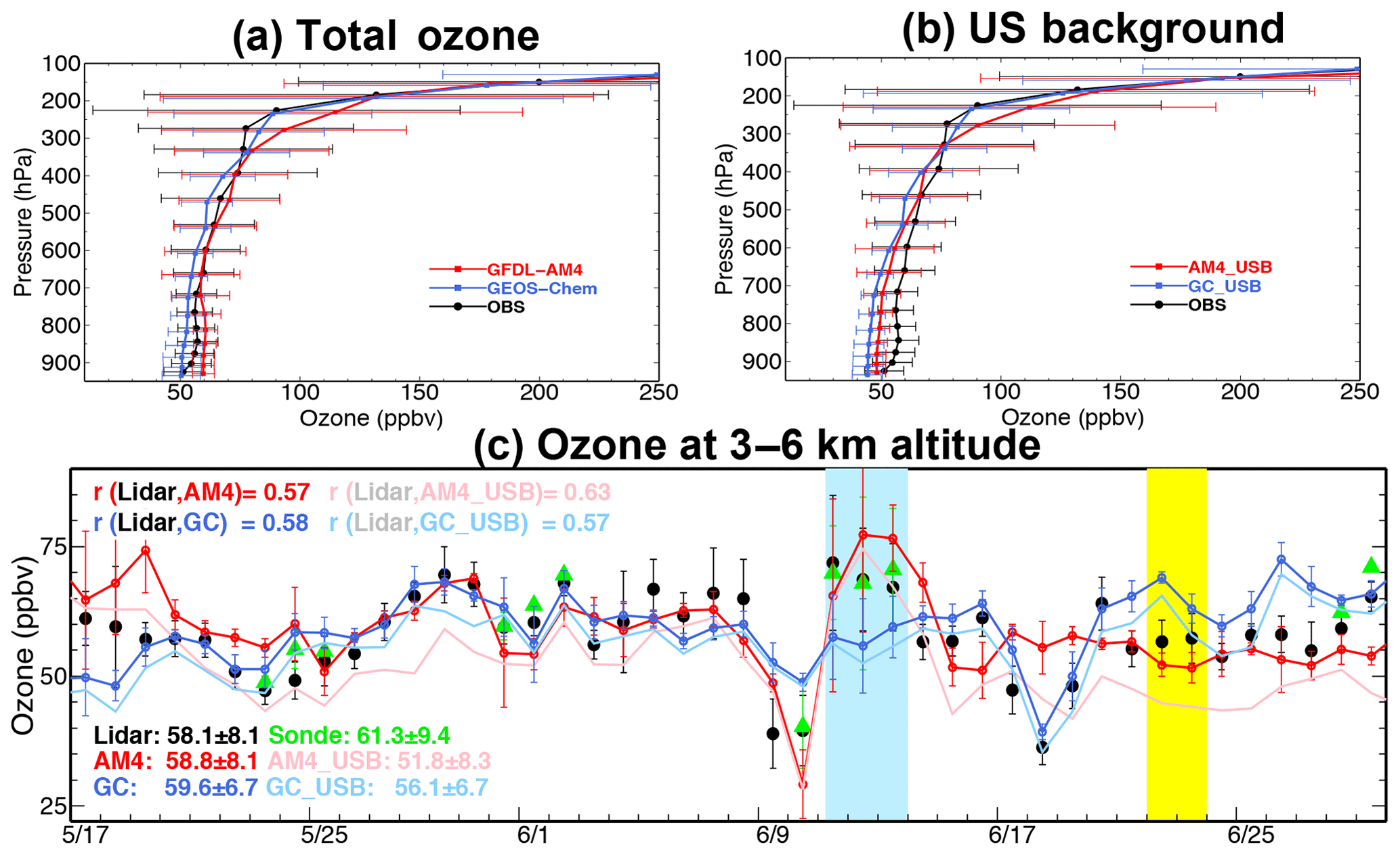
Figure 3(a) Mean vertical O3 profiles at Joe Neal as observed with ozonesondes (black; 30 launches) and simulated with GFDL-AM4 (red) and GEOS-Chem (blue) during FAST-LVOS (May–June 2017). Horizontal bars represent the standard deviations across daily profiles; (b) Same as (a) but showing US background (USB) O3 estimated by the two models. (c) Time series of O3 averaged over 3–6 km altitude above NLVA during FAST-LVOS as observed (black: lidar; green: ozonesonde) and simulated with GFDL-AM4 (thick red line) and GEOS-Chem (thick dark blue line), together with simulated USB O3 (light lines). Here and in other figures, AM4_USB represents USB estimated by GFDL-AM4 and GC_USB represents USB estimated by GEOS-Chem. The blue shading highlights the period with stratospheric intrusions and the yellow shading, the wildfire event. Vertical bars represent the standard deviations across hourly averages.
Figure 4 shows the time series of observed and simulated surface MDA8 O3 at four high-elevation sites and one low-elevation site in the region during the study period. Statistics comparing the results at all sites are shown in Table S1. The two models show large differences in simulated total and USB O3 on days when the O3Strat tracer in AM4 indicates stratospheric influence (highlighted in blue shading). AM4 O3Strat indicates frequent STT events during April–June, with observed MDA8 O3 exceeding or approaching the current NAAQS of 70 ppbv. Compared with observations, GFDL-AM4 captures the spikes of MDA8 O3 and elevated USB O3 during these STT events (e.g., 23 April, 13 May, and 11 June). On these days, GEOS-Chem underestimates observed O3 by 10–25 ppbv and simulates much lower USB O3 levels than GFDL-AM4. For some days, GFDL-AM4 overestimates total MDA8 O3 due to excessive STT influence (e.g., 7 May at Spring Mountain Youth Camp). The two models also differ substantially in total and USB O3 (14–18 ppbv) on 22 June (yellow shading), with GEOS-Chem overestimating observations at high-elevation sites, while GFDL-AM4 underestimates observations at both high- and low-elevation sites. We provide more in-depth analysis of these events in Sect. 4 and identify the possible causes of the model biases.
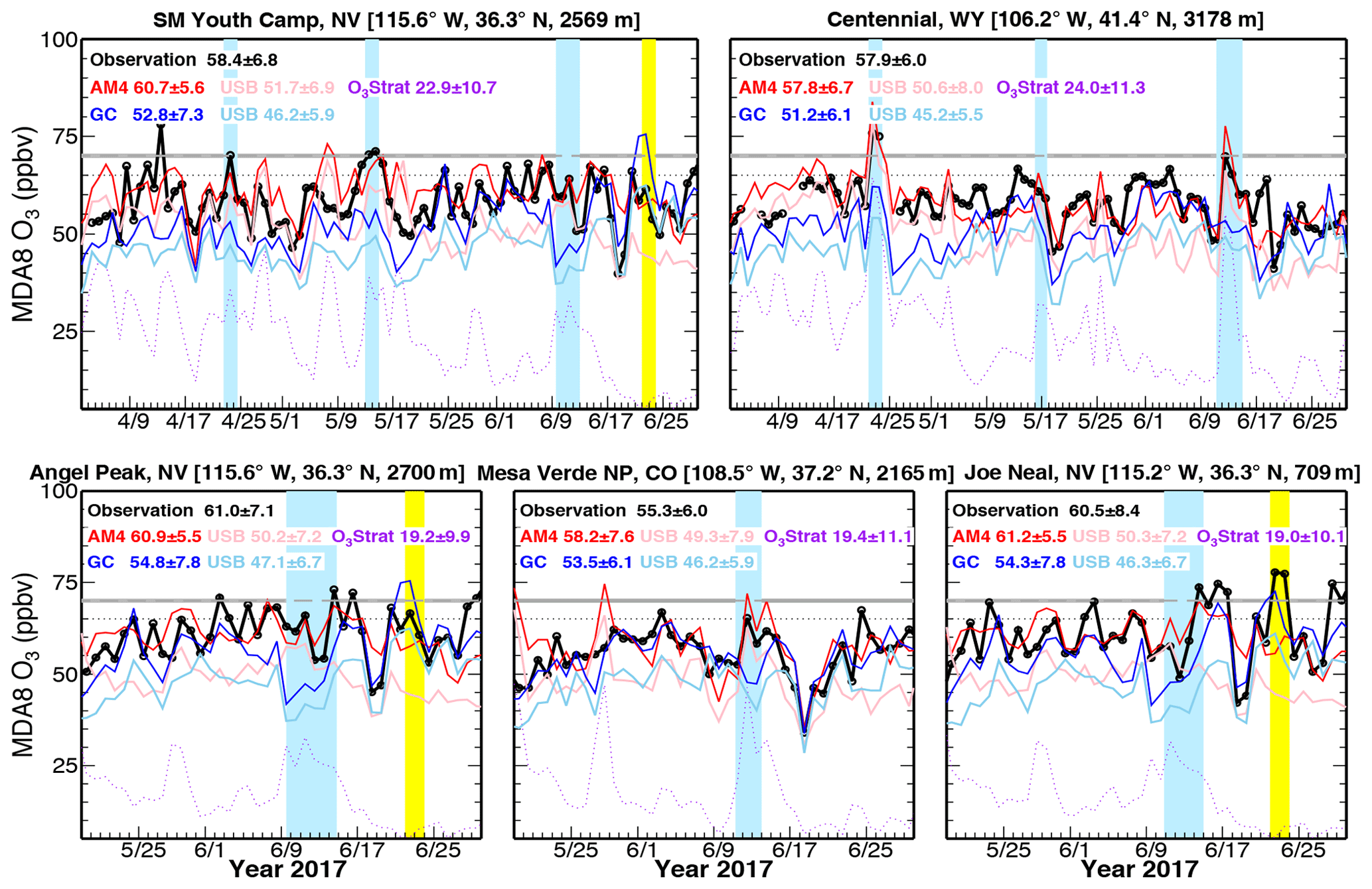
Figure 4Time series of daily MDA8 O3 at Spring Mountain Youth Camp (SMYC) in Nevada and Centennial in Wyoming from April to June and at Angel Peak, Mesa Verde, and Joe Neal during the FAST-LVOS study period, highlighting stratospheric intrusion events (blue shading) and wildfire events (yellow shading). The SMYC O3 monitor is located only about 125 m below and 800 m west of the Angel Peak summit where the mobile lab was parked. Shown are total MDA8 O3 from observations (black) and simulations by GFDL-AM4 (red) and GEOS-Chem (blue), together with USB O3 from GFDL-AM4 (pink) and GEOS-Chem (light blue). The dashed purple line shows AM4 stratospheric O3 tracers The horizontal lines denote the current NAAQS level of 70 ppbv and a possible future standard of 65 ppbv.
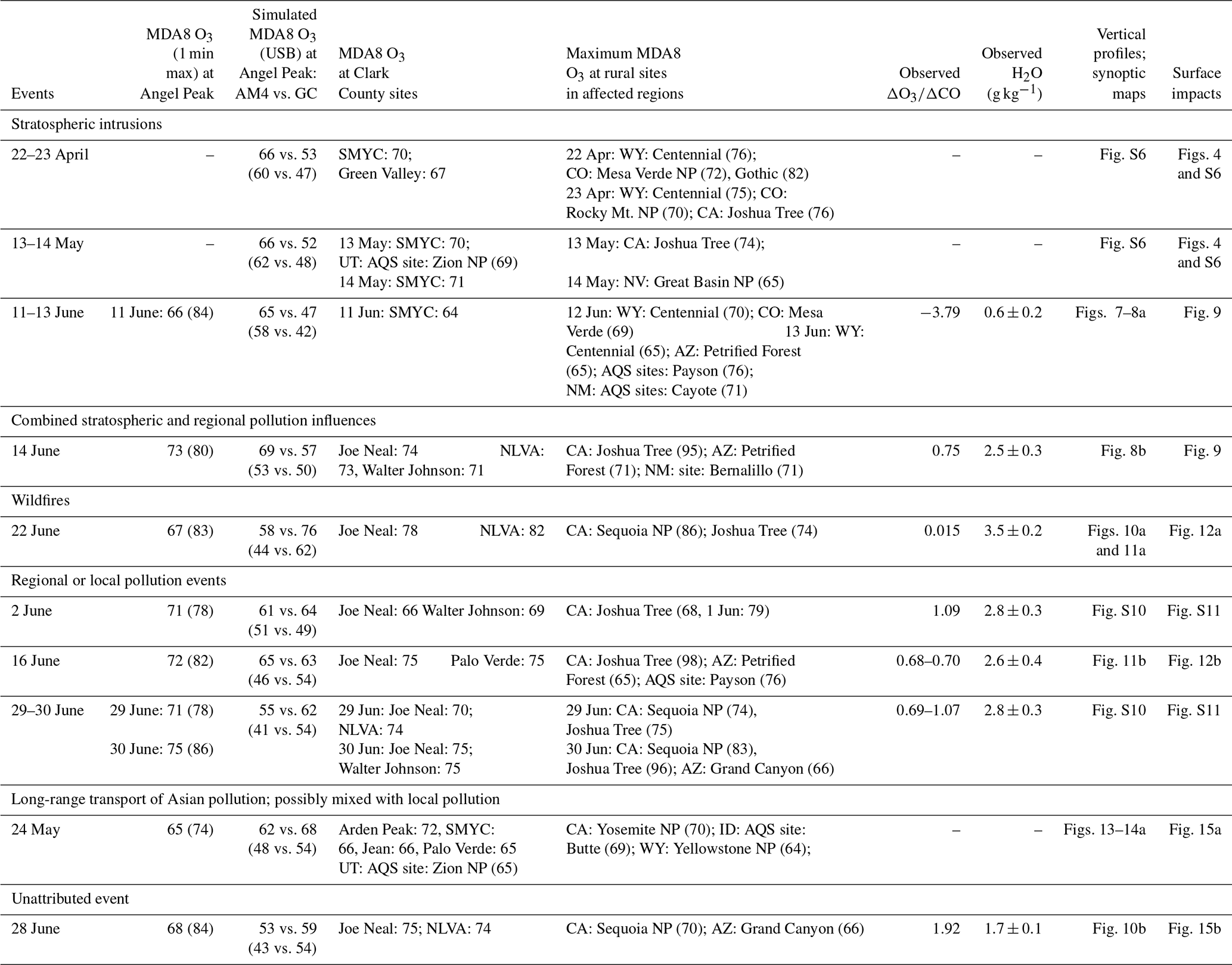
We identify 10 events with observed MDA8 O3 exceeding 65 ppbv at multiple sites in the greater Las Vegas area during April–June 2017. Table 1 provides an overview of the events, the dominant source for each event, the surface sites impacted, and the associated analysis figures presented in this article. Observations and model simulations of MDA8 O3 for each event are also included in Table 1 for Angel Peak and in Table S4 and Fig. S4 for all Clark County surface sites. The attribution is based on a combination of observational and modeling analyses. First, we examine the relationships and collocated meteorological measurements from the NOAA/ESRL mobile lab deployed at Angel Peak to provide a first guess on the possible sources of the observed high-O3 events (Sect. 4.1). Then, we analyze large-scale meteorological fields (e.g., potential vorticity), satellite images (e.g., AIRS CO), and lidar and ozonesonde observations to examine if the transport patterns, the high-O3 layers, and related tracers are consistent with the key characteristics of a particular source (Sect. 4.2–4.5). Available aerosol backscatter measurements and multi-tracer aircraft profiles are also used to support the attribution (Sect. 4.3 and 4.6). Finally, for each event we examine the spatiotemporal correlations of model simulations of total O3, background O3, and its components (e.g., stratospheric ozone tracer), both in the free troposphere and at the surface. For a source to be classified as the dominant driver of an event, O3 from that source must be elevated sufficiently from its mean baseline value.
Table 1List of high-O3 events above 65 ppbv in the greater Las Vegas region during April–June 2017 (unit: ppbv).
4.1 Observed relationships
Relationships between concurrently measured O3 and CO are useful to identify the possible origins of elevated surface O3 (Parrish et al., 1998; Herman et al., 1999; Langford et al., 2015). During FAST-LVOS, in situ 1 min measurements at Angel Peak show differences in ΔO3∕ΔCO and water vapor content between air plumes during a variety of events (Figs. 5, 6, and S5). Notably, on 11 June, O3 was negatively correlated with CO (ΔO3∕ΔCO = −3.79). This anti-correlation is distinctly different from the O3/CO relationships during other periods (e.g., ΔO3∕ΔCO = 0.68–0.70 on 16 June or ΔO3∕ΔCO = 1.08 on 2 June). The negative correlation (high O3 together with low CO) serves as strong evidence of a stratospheric origin of the air masses on 11 June, since O3 is much more abundant in the stratosphere than in the troposphere, whereas CO is mostly concentrated within the troposphere where it is directly emitted or chemically formed (Langford et al., 2015). By contrast, simultaneously elevated O3 and CO suggest influences by wildfires (e.g., 22 June) or anthropogenic (e.g., 16 June) pollution (Figs. 6b–d and S4). In particular, exceptionally high CO levels (∼100–440 ppbv) on 22 June (Fig. 6e) suggest influences from wildfires. Ozone enhancements were measured by the TOPAZ ozone lidar on 22 June (Sect. 4.3), although the correlation between CO and O3 at Angel Peak is not strong. The net production of O3 by wildfires is highly variable, with many contradictory observations reported in the literature (Jaffe and Wigder, 2012). The amount of O3 within a given smoke plume varies with distance from the fire and depends on the plume injection height, smoke density, and cloud cover (Faloona et al., 2020).
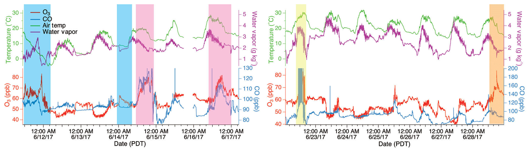
Figure 5Time series of 1 min averaged air temperature, water vapor, O3, and CO mixing ratios measured by the NOAA mobile lab deployed at Angel Peak during 11–16 June and 22–28 June 2017, highlighting the periods with stratospheric influence (blue), regional anthropogenic pollution plumes (pink), wildfire plumes (yellow), and the unattributed pollution plume (orange). Data are shown in Pacific daylight time (PDT). Note that peak CO mixing ratios on 22 June were 440 ppbv (not shown on the plot).
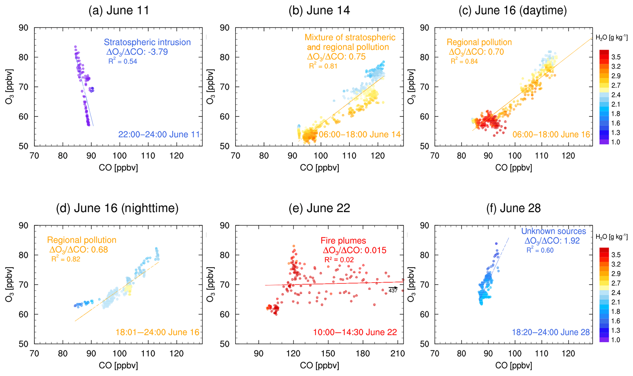
Figure 6Scatterplots of 1 min average O3 against CO measured at Angel Peak, color-coded by specific humidity, for air masses influenced by (a) STT on 11 June; (b) regional pollution on 14 June; (c–d) regional pollution plume during daytime (06:00–18:00) and nighttime (18:01–24:00) on 16 June; (e) wildfires on 22 June; and (f) unattributed pollution on 28 June. Note that peak CO mixing ratios on 22 June were 440 ppbv (not shown on the plot).
We gain further insights by examining water vapor concurrently measured at Angel Peak. Air masses from the lower stratosphere are generally dry, whereas wildfire or urban plumes from the boundary layer are relatively moist (Langford et al., 2015). Thus, the dry conditions of the air masses on 11 June support our conclusion that the plume was transported downward from the upper troposphere and lower stratosphere (Fig. 6a). These conditions are in contrast to those of the urban or wildfire plumes transported from the Las Vegas Valley (Fig. 6c–d). Additionally, we separate the anthropogenic plumes on 16 June into daytime and nighttime conditions because of a diurnal variation in air conditions (relatively dry at night versus wet during daytime; Fig. 6c–d). This analysis further demonstrates that the anthropogenic pollution plume during nighttime is wetter than the stratospheric air on 11 June. On 14 June (Fig. 6b), measured O3 was positively correlated with CO, indicating regional or local pollution influence, but the lower levels of water vapor than those in regional pollution and wildfire plumes suggest that the stratospheric air which reached Angel Peak earlier may have been mixed with local pollution. On 28 June (Fig. 6f), O3 was positively correlated with CO and the air masses were relatively dry, indicating that the plume was likely from aged pollution transported from Asia or southern California as opposed to from fresh pollution from the Las Vegas Valley. Identifying the primary source of the high-O3 events solely based on observations is challenging; additional insights from models are thus needed as we demonstrate below.
4.2 Characteristics of stratospheric intrusion during 11–14 June
Analysis of the 250 hPa potential vorticity and the AM4 model stratospheric O3 tracer shows significant stratospheric influence on surface O3 in the SWUS on 22–23 April (Fig. S6), 13–14 May (Fig. S6), and 11–14 June (Figs. 7–8). During these events, surface MDA8 O3Strat in AM4 was 20–40 ppbv higher than the mean baseline level (15–20 ppbv; see dashed purple lines Fig. 4). Below, we focus on the 11–14 June event, which was the subject of a 4 d FAST-LVOS IOP with 60 h of continuous O3 lidar profiling and 13 ozonesonde launches, in addition to continuous in situ measurements at Angel Peak.
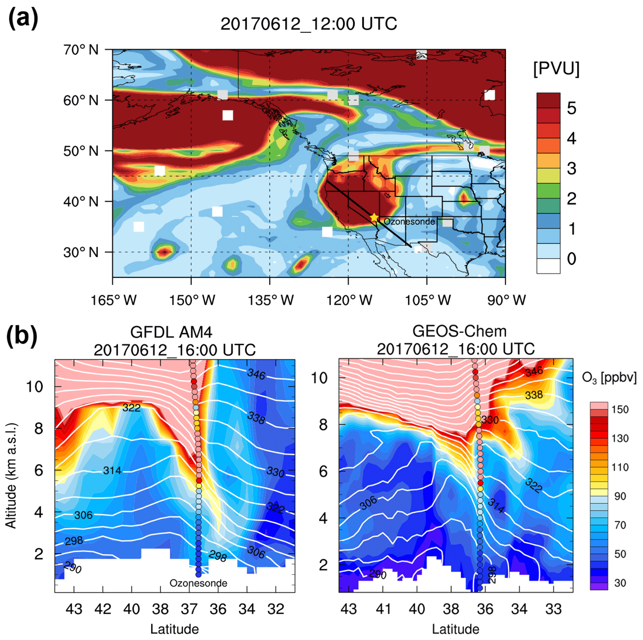
Figure 7(a) Potential vorticity at 250 hPa on 12 June calculated from the NCEP-Final (FNL) reanalysis (PVU: 10−6 m2 s−1 K kg−1); (b) vertical distributions of O3 (color shading) and isentropic surfaces (white lines) along a transect crossing Nevada (black line on PV map) simulated with GFDL-AM4 (left) and GEOS-Chem (right) on 12 June. The color-coded circles denote ozonesonde observations at Joe Neal (star on the PV map).
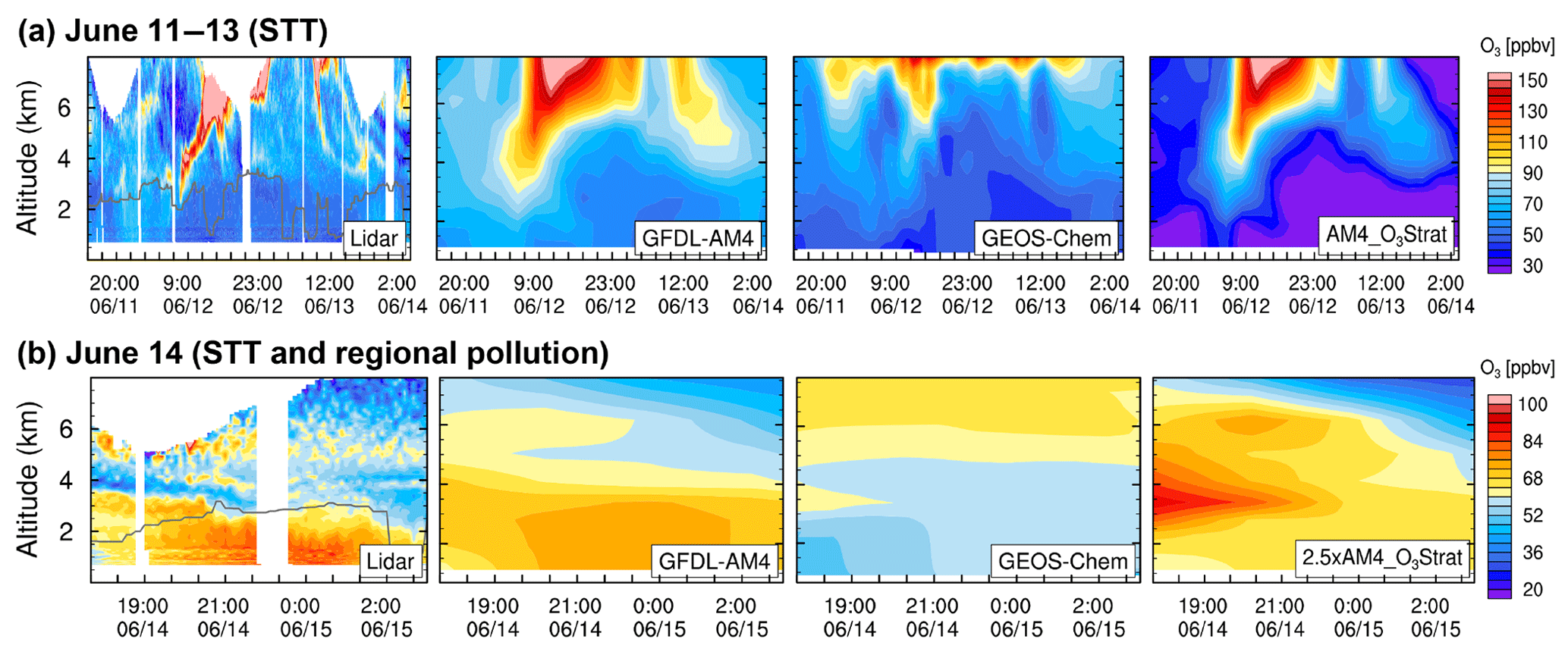
Figure 8Time–height curtain plots of O3 above NLVA as observed with TOPAZ lidar and simulated with GFDL-AM4 (∼50 km × 50 km; interpolated from 3-hourly data) and GEOS-Chem (0.25∘ × 0.3125∘; interpolated from hourly data) during the STT event on (a) 11–13 June and (b) 14 June 2017 (UTC). The rightmost panel shows the AM4 stratospheric O3 tracer (AM4_O3Strat). Note that AM4 O3Strat for 14 June is scaled by a factor of 2.5 for clarity. Here and in other figures, the solid black lines in the O3 lidar plots represent boundary layer height inferred from the micro-Doppler lidar measurements.
4.2.1 Deep stratospheric intrusion on 11–13 June
Synoptic-scale patterns of potential vorticity (PV) indicate a strong upper-level trough over the northwest US on 12 June (Fig. 7a). The PV pattern displays a “hook-shaped” streamer of air extending from the northern US to the Intermountain West, a typical feature for an STT event (Lin et al., 2012a; Akritidis et al., 2018). This upper-level trough penetrated southeastwardly towards the SWUS, facilitating the descent of stratospheric air masses into the lower troposphere. Ozonesondes launched at Joe Neal on 12 June recorded elevated O3 levels of 150–270 ppbv at 5–8 km altitude (color-coded circles in Fig. 7b). Consistent with the ozonesonde measurements, GFDL-AM4 shows that O3-rich stratospheric air masses descended isentropically towards the study region, with simulated O3 reaching 90 ppbv at ∼2 km altitude. For comparison, GEOS-Chem simulates a much weaker and shallower intrusion (Fig. 7b), despite a similar synoptic-scale pattern of potential vorticity at 250 hPa and comparable ozone levels in the upper troposphere–lower stratosphere (Fig. S7), suggesting possibly greater numerical diffusion in GEOS-Chem diluting the stratospheric intrusion. There are also some notable differences in the isentropic surfaces (e.g., at 322 K) between the two models, possibly resulting from a difference in the two meteorological reanalysis data (NCEP in AM4 and MERRA in GEOS-Chem).
TOPAZ lidar measurements at NLVA vividly characterize the strength and vertical depth of intruding O3 tongues evolving with time (Fig. 8a). A tongue of high O3 exceeding100 ppbv descended to as low as 2–3 km altitude on 12 June. GFDL-AM4 captures both the timing and structure of the observed high-O3 layer and attributes it to a stratospheric origin as supported by the O3Strat tracer. In contrast, GEOS-Chem substantially underestimates the depth and magnitude of the observed high-O3 layers in the free troposphere. Zhang et al. (2014) also showed that GEOS-Chem captures the timing of stratospheric intrusions but underestimates their magnitude by a factor of 3.
Surface observations show that high MDA8 O3 exceeding 60 ppbv first emerged on 11 June over southern Nevada (Fig. 9), consistent with the arrival of stratospheric air masses as inferred from the negative correlation between O3 and CO measured at Angel Peak (Fig. 6a). Over the next few days, the areas with observed MDA8 O3 approaching 70 ppbv gradually shifted southward from Nevada and Colorado to Arizona and New Mexico. By 13 June, observed surface MDA8 O3 exceeded 70 ppbv over a large proportion of the SWUS, including Arizona and New Mexico. GFDL-AM4 captures well the observed day-to-day variability of high-O3 spots over the WUS, although the model overall has high biases. Over the areas where observed MDA8 O3 levels are 60–75 ppbv, GFDL-AM4 estimates 50–65 ppbv USB O3 with simulated O3Strat 20–40 ppbv higher than its mean baseline level in June. GEOS-Chem has difficulty simulating the observed high-O3 areas during this event, and simulated USB is 15 ppbv lower than AM4 (Fig. 9). These results are consistent with the fact that GEOS-Chem does not capture the structure and magnitude of deep stratospheric intrusions during the period (Figs. 3, 7, and 8).
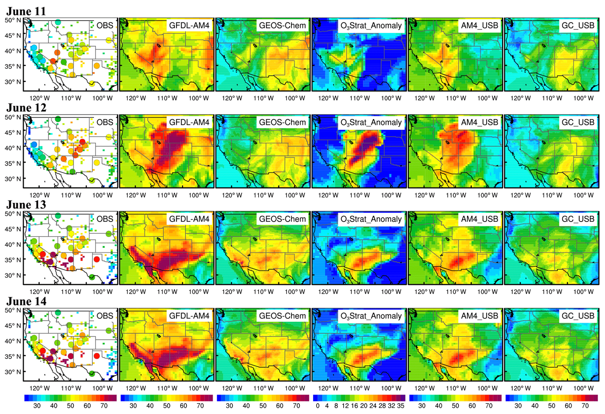
Figure 9Maps of total MDA8 O3 (ppbv) in surface air as observed (small squares for AQS data and large circles for CASTNet data) and simulated with GFDL-AM4 and GEOS-Chem, along with anomalies in AM4 O3Strat (relative to June mean) and model-estimated USB levels, during the STT event on 11–14 June 2017. Note that O3Strat in this figure and Fig. S6 is shown as anomalies relative to the monthly mean, while the absolute values are shown in Figs. 4 and 8.
4.2.2 Mixing of stratospheric ozone with regional pollution on 14 June
Stratospheric air masses that penetrate deep into the troposphere can mix with regional anthropogenic pollution and gradually lose their typical stratospheric characteristics (cold and dry air containing low levels of CO), challenging the diagnosis of stratospheric impacts based directly on observations (Cooper et al., 2004; Lin et al., 2012b; Trickl et al., 2016). On 14 June, O3 measured at Angel Peak is positively correlated with CO (ΔO3∕ΔCO = 0.75; Fig. 6b), similar to conditions of anthropogenic pollution on 16 June (Fig. 6c–d). TOPAZ lidar shows elevated O3 of 70–80 ppbv concentrated within the boundary layer below 3 km altitude (Fig. 8b). These observational data do not provide compelling evidence for stratospheric influence. However, GFDL-AM4 simulates elevated O3Strat coinciding with the observed and modeled total O3 enhancements within the planetary boundary layer (PBL), indicating that O3 from the deep stratospheric intrusion on the previous day may have been mixed with regional anthropogenic pollution to elevate O3 in the PBL. At the surface (the bottom panels in Fig. 9), AM4 simulates high USB O3 and elevated O3Strat (20–40 ppbv above its mean baseline) over Arizona and New Mexico where MDA8 O3 greater than 70 ppbv was observed. The fact that GEOS-Chem is unable to simulate the ozone enhancements in lidar measurements and at the surface further supports the possible stratospheric influence. This case study demonstrates the value of integrating observational and modeling analysis for the attribution of high-O3 events over a region with complex O3 sources.
The extent to which stratospheric intrusions contribute to surface O3 at low-elevation sites over the WUS has been poorly characterized in previous studies. Notably, surface O3 at three low-elevation (∼700–800 m a.s.l.) air quality monitoring sites in Clark County exceeded the current NAAQS level of 70 ppbv on 14 June: 74 ppbv at Joe Neal, 73 ppbv at North Las Vegas Airport, and 71 ppbv at Walter Johnson. The number of monitoring sites with O3 exceedances would have increased to 11 in Clark County if the NAAQS had been lowered to 65 ppbv. While O3 produced from regional anthropogenic emissions still dominates pollution in the Las Vegas Valley (Fig. S4), our analysis shows that stratospheric intrusions can mix with regional pollution to push surface O3 above the NAAQS.
4.3 Wildfires on 22 June
Significant enhancements in aerosol backscatter were observed at 3–6 km altitude above NLVA on 21–22 June, indicating the presence of wildfire smoke (Fig. 10a). Under the influence of the wildfire plume, mobile lab measurements at Angel Peak (∼3 km altitude) detected elevated CO as high as 440 ppbv in warm, moist air masses (Fig. 6e). The lidar measurements at NLVA on 22 June showed broad O3 enhancements (80–100 ppb) from the surface to 4 km altitude (Fig. 11a). After 12:00 PDT (19:00 UTC), a deep PBL (3–4 km) developed and O3 within the PBL was substantially enhanced (>80 ppbv), likely due to strong O3 production through reactions between abundant VOCs in the wildfire plumes and NOx in urban environments (Singh et al., 2012; Gong et al., 2017). Surface MDA8 O3 exceeded 70 ppbv at multiple sites in the Las Vegas Valley during the event (Table 1). Unfortunately, the synoptic conditions did not trigger an IOP, so there were no aircraft or ozonesonde measurements during this event.
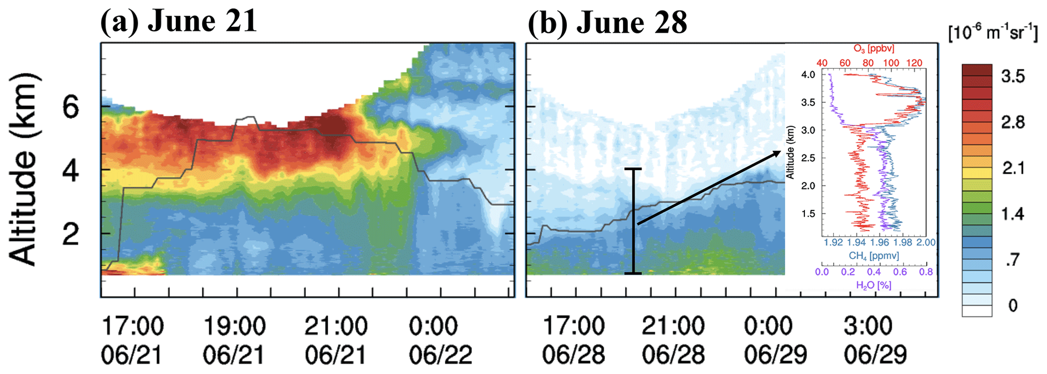
Figure 10Time–height curtain plots of the TOPAZ aerosol backscatter above the North Las Vegas Airport during 21–22 June (a) and 28 June 2017 (b). Data are shown at UTC time. The inset graph in (b) shows vertical profiles of water vapor (purple), CH4 (blue), and O3 (red) measured by the Scientific Aviation flight above the Las Vegas Valley during 19:15–19:35 28 June (UTC) (flight track in Fig. 1).
GFDL-AM4 has difficulty simulating the O3-rich plumes above Clark County on 22 June (Fig. 11a). GEOS-Chem captures the observed high-O3 layers within the PBL but overestimates O3 above 4 km altitude (Fig. 11a). GEOS-Chem overestimates of free-tropospheric ozone seem to be common for the non-STT events during late spring through summer (Figs. 3b, 8b, and 11b and comparisons with lidar data for 24 May and 16 June shown in Sect. 4.4–4.6), likely due to excessive O3 produced from lightning NOx over the southern US (Zhang et al., 2011, 2014). At the surface, total MDA8 O3 concentrations simulated by the two models bracket the observed values at sites in the Las Vegas area (see yellow shading in Fig. 4) and across the Intermountain West (Fig. 12a). AM4 does not simulate elevated O3 during this event, while GEOS-Chem simulates elevated total and USB O3 levels across the entire southwest region. GEOS-Chem simulations during this wildfire event agree better with the observed MDA8 O3 enhancements (>70 ppbv) at Joe Neal (Fig. 4). At the high-elevation sites Angel Peak and Spring Mountain Youth Camp, however, GEOS-Chem overestimates the observed MDA8 O3 by 10–15 ppbv. Overall, GEOS-Chem seems to be more consistent with observations than GFDL-AM4 during this wildfire event. However, we cannot rule out the possibility that the better agreement between observations and GEOS-Chem simulations during this event may reflect excessive O3 from lightning NOx in the model (Zhang et al., 2014).
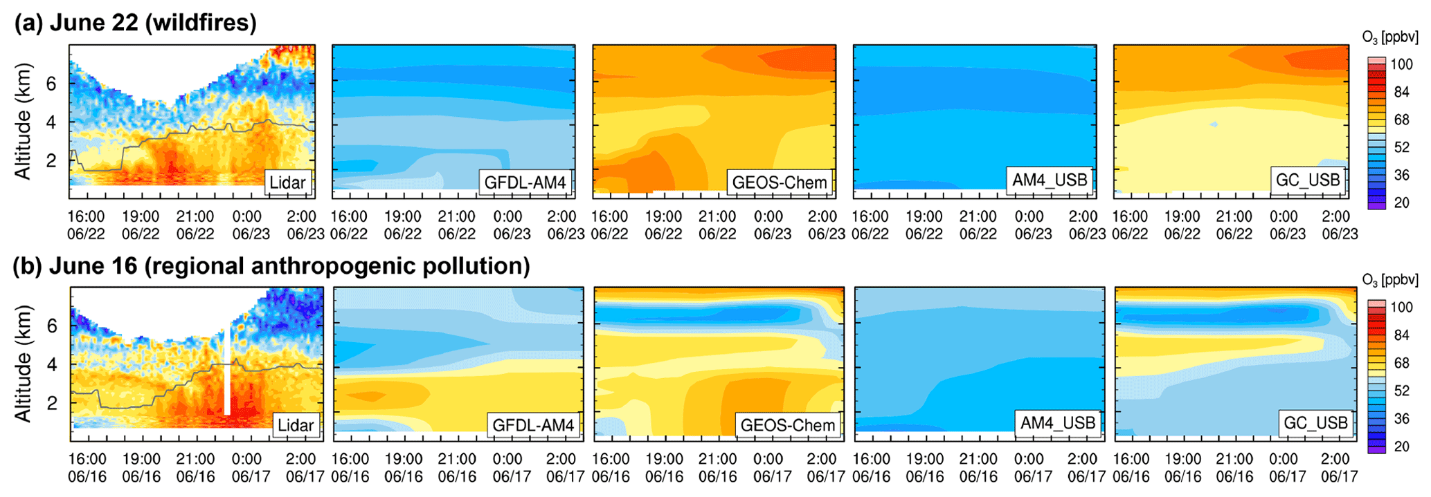
Figure 11Same as Fig. 8 but for (a) the wildfire event on 22 June and (b) the regional anthropogenic pollution event on 16 June 2017 (UTC). The right panels compare USB O3 from the two models.
Meteorological conditions (e.g., temperature and wind fields) on 22 June in the reanalysis data used by GFDL-AM4 and GEOS-Chem are similar over the WUS (not shown). The two models use the same wildfire emissions (FINN) but with different vertical distributions. Fire emissions are distributed between the surface and 6 km altitude in GFDL-AM4 but are placed at the surface level in GEOS-Chem. We conduct several sensitivity simulations with GFDL-AM4 to investigate the causes of the model biases. Placing all fire emissions at the surface in GFDL-AM4 results in ±5 ppbv differences in modeled MDA8 O3 on 22 June (Fig. S8). Observations suggested that 40 % of NOx can be converted rapidly to peroxyacyl nitrate (PAN) and 20 % to HNO3 in fresh boreal fire plumes over North America (Alvarado et al., 2010). Both models currently treat 100 % of wildfire NOx emissions as NO. We conduct an additional AM4 sensitivity simulation, in which 40 % of the wildfire NOx emissions are released as PAN and 20 % as HNO3. This treatment results in ±2 ppbv differences in simulated monthly mean MDA8 O3 during an active wildfire season (August 2012; Fig. S9). Overall, these changes do not substantially improve simulated O3 on 22 June. Future efforts are needed to investigate the ability of current models to simulate O3 formations in fire plumes (Jaffe et al., 2018).
4.4 Regional and local anthropogenic pollution events
Regional and local anthropogenic emissions were important sources of elevated O3 in Clark County during FAST-LVOS, contributing to 3 out of 10 observed high-O3 events above 65 ppbv during April–June 2017 (Table 1). Below, we focus on the 16 June event when severe O3 pollution with MDA8 O3 exceeding 70 ppbv occurred over California, Arizona, parts of Nevada, and New Mexico. Analysis for the 2 and 29–30 June pollution events are shown in the Supplement (Figs. S5, S10, and S11). The TOPAZ lidar measurements on 16 June show elevated O3 of 55–90 ppbv in the 4 km deep PBL (Fig. 11b). However, this event did not trigger an IOP, so ozonesonde and aircraft measurements are unavailable. Both GFDL-AM4 and GEOS-Chem capture the buildup of O3 pollution in the PBL on 16 June (Fig. 11b). Both models show boundary layer enhancements of total O3 but not of USB O3 (Fig. 11b), indicating that regional or local anthropogenic emissions are the primary source of observed O3 enhancements. Similar to 16 June, GEOS-Chem clearly shows enhancements in total O3 in the PBL but not in USB O3 on 2 and 29–30 June (Fig. S10). The model attribution to US anthropogenic emissions is consistent with the positive correlation between O3 and CO measured at Angel Peak on 16 (Fig. 6c–d), 2, and 29–30 June (Fig. S5). It is noteworthy that, with its higher horizontal resolution, GEOS-Chem better resolves the structure of the O3 plumes as observed by the TOPAZ lidar for all the three pollution events. At the surface, both models capture the large-scale MDA8 O3 enhancements across the SWUS on 16 June (Fig. 12b). The surface O3 enhancements on 2 and 29–30 June are relatively localized in southern California and the Las Vegas area (Fig. S11), and both models have difficulty simulating the observed peak MDA8 values (Fig. 4).
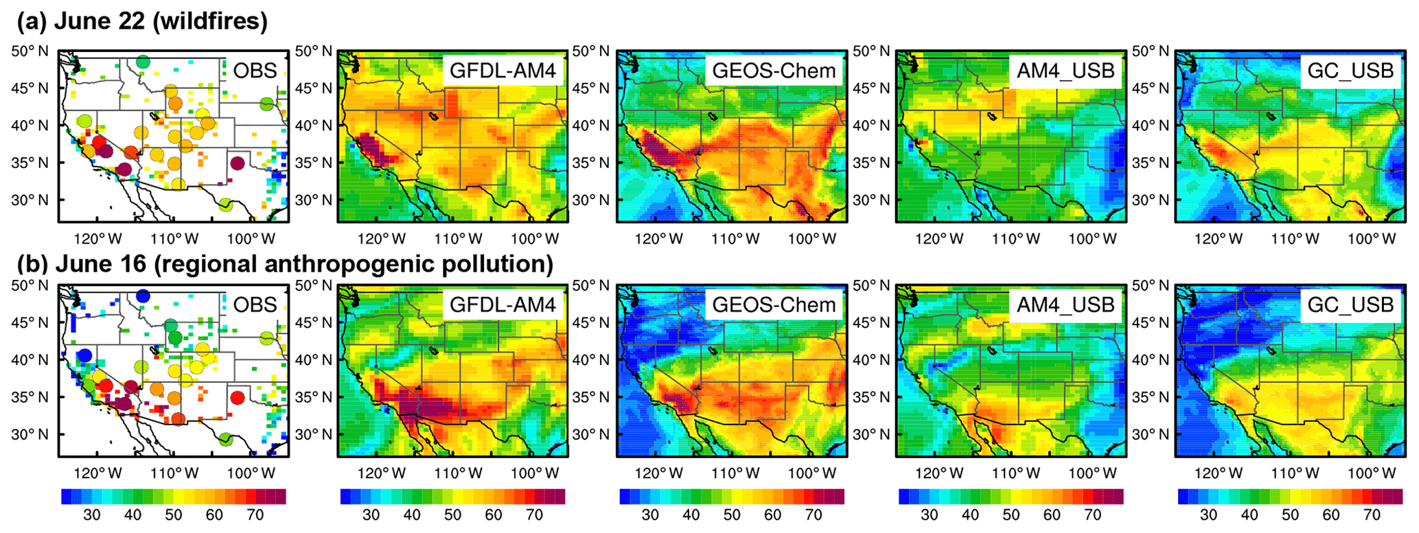
Figure 12Same as Fig. 9 but for (a) the wildfire event on 22 June and (b) the regional anthropogenic pollution event on 16 June 2017.
4.5 Long-range transport of Asian pollution on 20–24 May
During 20–24 May, long-range transport of Asian pollution toward the WUS was observed via large-scale CO column observations with the Atmospheric Infrared Sounder (AIRS) on NASA's Aqua satellite (Fig. 13a). These Asian plumes traveled eastward across the Pacific for several days, reaching the west coast of the US on 23 May during the first FAST-LVOS IOP (23–25 May). The lidar measurements at NLVA on 24 May clearly showed high-O3 plumes (>70 ppbv) concentrated within layers of 1–4 km and 6–8 km altitude above the Las Vegas Valley throughout the day (Fig. 14a). Both GFDL-AM4 and GEOS-Chem capture the observed O3-rich plumes at surface–4 km and 6–8 km altitude above Clark County during this event. Elevated O3 at 6–8 km altitude reflects the long-range transport from Asia, as supported by concurrent enhancements in total and USB O3 in both models and by the large difference in O3 between the AM4 BASE simulation and the sensitivity simulation with Asian anthropogenic emissions zeroed out. Elevated O3 at 1–4 km altitude appears to be influenced by a residual pollution layer from the previous day; this plume was later mixed into the growing PBL (up to 4 km altitude), elevating MDA8 O3 in surface air on 24 May. Further supporting the impact from regional or local pollution below 4 km altitude, both models simulate much larger enhancements in total O3 (70–90 ppbv) than in USB O3 (∼50 ppbv).
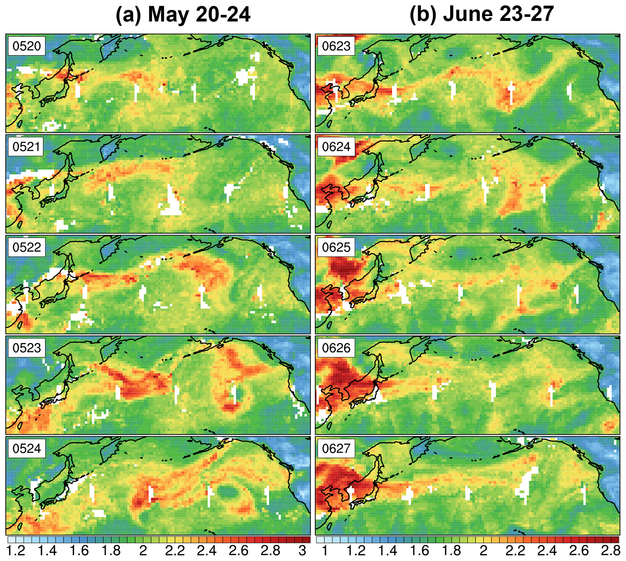
Figure 13Trans-Pacific transport of Asian pollution plumes during (a) 20–24 May and (b) 23–27 June 2017, as seen in the NASA AIRS retrievals of CO total column (1018 molecules cm−2; level 3 daily 1∘ × 1∘ gridded products).

Figure 14Same as Fig. 8 but for (a) the Asian pollution event on 24 May and (b) the unattributed pollution event on 28 June 2017 (UTC).
On 24 May, MDA8 O3 approached or exceeded the 70 ppbv NAAQS at multiple sites in California, Idaho, Wyoming, and Nevada (Fig. 15a), likely reflecting the combined influence of regional pollution and long-range transport of Asian pollution. MDA8 O3 at four surface sites in Clark County was above 65 ppbv. More exceedances would have occurred if the level for the NAAQS were lowered to 65 ppbv. In parts of Idaho, Wyoming, and California where observed MDA8 O3 was higher than 60 ppbv, the contribution of Asian anthropogenic emissions as estimated by GFDL-AM4 was 8–15 ppbv (Fig. 15a), much higher than the springtime average contribution of ∼5 ppbv estimated by previous studies (e.g., Lin et al., 2012b), supporting the episodic influence from Asian pollution during this event. At several high-elevation sites in California such as Arden Peak (72 ppbv) and Yosemite National Park (70 ppbv), where observed MDA8 O3 exceeds the NAAQS level, the contribution of Asian pollution is approximately 9 ppbv. Ozone produced from regional and local anthropogenic emissions dominates the observed MDA8 O3 above 70 ppbv in the Central Valley of California.
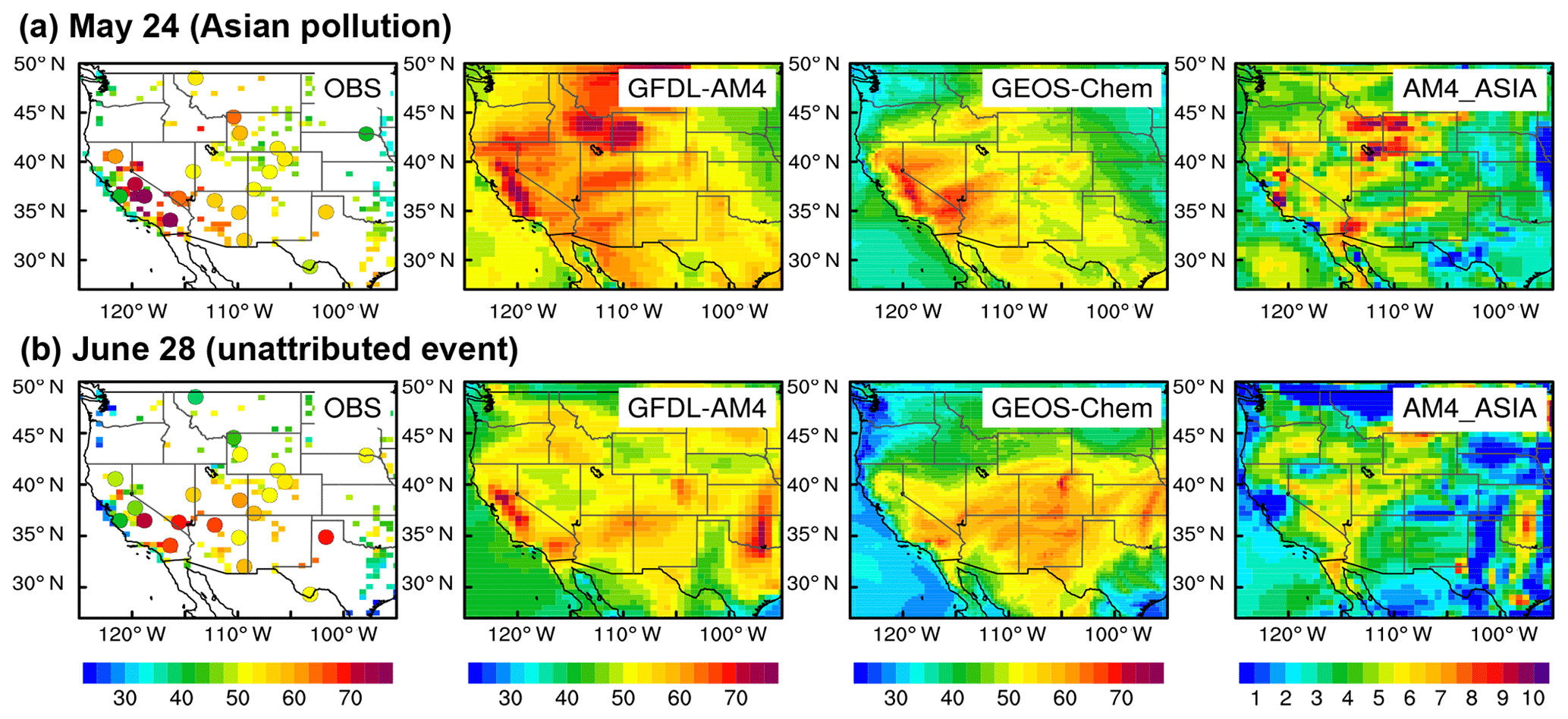
Figure 15Same as Fig. 9 but for (a) the Asian pollution event on 24 May and (b) the unattributed pollution event on 28 June 2017. The right panels show O3 enhancements from Asian pollution estimated by GFDL-AM4.
4.6 An unattributed event: 28 June
The lidar measurements from 28 June show a fine-scale structure with a narrow O3 layer exceeding 100 ppbv at 3–4 km altitude during 08:00–14:00 PDT (15:00–21:00 UTC shown in Fig. 14b). An ozonesonde launched at 12:00 PDT also detected a high-O3 layer (∼115 ppbv) between 3.5 and 4 km altitude (not shown). This high-O3 filament appears to descend and mix into the PBL after 14:00 PDT (21:00 UTC), contributing to elevated O3 within the PBL in the afternoon. Both models are unable to represent this fine-scale transport event, possibly due to diffusive mixing of the narrow layer (Fig. 14b). We, therefore, focus on available airborne and in situ measurements to investigate the origin of this fine-scale O3 filament.
Our examinations of large-scale satellite CO column measurements reveal a migration during 23–27 June of high-CO plumes from Asia that arrived at the west coast of the US on 27 June (Fig. 13b). GFDL-AM4 estimates 5–6 ppbv contributions from Asian pollution over the WUS on 28 June (Fig. 15b), which do not represent a significant enhancement above the mean Asian contribution. Aircraft measurements above the Las Vegas Valley in the late morning showed collocated enhancements in CH4 and O3 coincident with low free-tropospheric water vapor values at 3–4 km altitude (Fig. 10b). In situ measurements at Angel Peak show concurrent increases in CO and O3 coincident with relatively dry conditions that are consistent with transported Asian pollution, but these increases did not appear until several hours after the fine-scale filament was entrained by the mixed layer (Fig. 6f). These observations indicate that the O3-rich plume appears to be unrelated to stratospheric intrusions. Aerosol backscatter measurements at NLVA show only a slight enhancement in backscatter within the elevated O3 layer on 28 June, in contrast to the thick smoke observed on 22 June when the Las Vegas Valley was influenced by fresh wildfires (Fig. 10). HYSPLIT and FLEXPART analyses presented in Langford et al. (2020) suggest a possible connection to the Schaeffer Fire (https://en.wikipedia.org/wiki/Schaeffer_Fire, last access: 20 September 2019) in the Sequoia National Forest in California. Another possible source is the fine-scale lofting of pollution from southern California followed by transport into the free troposphere over Las Vegas (Langford et al., 2010). This event further demonstrates the complexity of O3 sources in the SWUS. We recommend measurements of atmospheric compounds like acetonitrile (CH3CN, abundant in fire plumes) and methyl chloride (CH3Cl, abundant in Asian pollution) (Holzinger et al., 1999; Barletta et al., 2009) via aircraft and in situ platforms in future field campaigns in the region to help identify the sources of such high-O3 filaments.
Here, we summarize the differences in total and background O3 between the two models over the WUS. GFDL-AM4 and GEOS-Chem differ in their spatial distributions and magnitudes of April–June mean USB O3 at the surface and in the free troposphere over the US (Figs. 16 and S12). USB O3 in GFDL-AM4 peaks over the high-elevation Intermountain West at the surface (45–55 ppbv; Fig. 16a) and over the northern US in the free troposphere (3–6 km altitude; 50–65 ppbv; Fig. 16b), due to stronger STT influence. In comparison, GEOS-Chem simulates higher USB O3 levels in southwestern states (e.g., Texas), both at the surface (45–50 ppbv) and at 3–6 km altitude (55–65 ppbv), likely due to excessive lightning NOx during early summer (Zhang et al., 2011, 2014; Fiore et al., 2014). The different north–south gradient in simulated USB between the two models (Figs. 16b and S12) likely reflects that GFDL-AM4 simulates stronger STT influences over the northwestern US, while GEOS-Chem produces greater O3 from lightning NOx emissions in the free troposphere over the southern US. Despite a quantitative disparity, both models simulate higher USB O3 levels over the WUS (45–55 ppbv in GFDL-AM4 and 35–45 ppbv in GEOS-Chem) than over the EUS at the surface (Fig. 16a). Our USB O3 estimates with GEOS-Chem are generally consistent with the estimates in previous studies using GEOS-Chem or regional models driven by GEOS-Chem boundary conditions (Zhang et al., 2011; Emery et al., 2012; Dolwick et al., 2015; Guo et al., 2018). In contrast to NAB O3 estimates in earlier studies by zeroing out North American anthropogenic emissions (Zhang et al., 2011, 2014; Lin et al., 2012a; Fiore et al., 2014), USB O3 estimates in our study include the additional contribution from Canadian and Mexican emissions. USB O3 at Clark County sites is ∼4 ppbv greater than NAB O3 in GFDL-AM4 (Table S5). We also find that NAB O3 estimated with the new GFDL-AM4 model is ∼5 ppbv lower than the NAB estimates by its predecessor GFDL-AM3 (Lin et al., 2012a) for the WUS during March–April (Fig. S13), consistent with an improved simulation of free-tropospheric ozone in AM4 during spring (Fig. 2). During early summer, the NAB O3 levels estimated by AM3 and AM4 are similar (Fig. S13).
We further compare simulated surface MDA8 O3 against observations at 12 high-elevation sites (>1500 m altitude; including 11 CASTNet sites and Angel Peak; see Table S1 and black circles in Fig. 1) in the WUS (Fig. 17). The observed high-MDA8-O3 events above 65 ppbv at these high-elevation sites are generally associated with enhanced background O3 in both models (USB O3 = 50–60 ppbv in GFDL-AM4 and 45–55 ppbv in GEOS-Chem; Fig. 17a). Stratospheric intrusions are an important source of the observed events above 65 ppbv (Fig. S14), as indicated by GFDL-AM4, which better captures these high-O3 events influenced by elevated background O3 contributions, whereas GEOS-Chem underestimates these extreme events (comparing points in the top-right box in Fig. 17a). Although AM4 is capable of simulating most of the highest observed springtime MDA8 O3 events (>65 ppbv) over the WUS, we note that AM4 tends to overestimate stratospheric influence on days when observed MDA8 O3 is in the range of 50–65 ppbv. For mean MDA8 O3 at these sites, GFDL-AM4 is biased high by 3 ppbv, while GEOS-Chem is biased low by 5 ppbv. Mean USB O3 simulated with GFDL-AM4 is 51.4±7.8 ppbv at WUS sites, higher than that in GEOS-Chem (45.7±5.7 ppbv; Fig. 17b). Probability distributions show that GFDL-AM4 simulates a wider range of total and USB O3 than GEOS-Chem, reflecting relative skill in capturing the day-to-day variability of O3. In addition to background O3 discussed in the present study, recent studies also found that ozone dry deposition coupled to vegetation can substantially influence model simulations of surface O3 means and extremes (Lin et al., 2019, 2020).
Tables S5 and S6 report year-to-year variability in the percentage of site days with springtime MDA8 O3 above 70 ppbv (or 65 ppbv) and simulated USB levels during 2010–2017. The percentage of site days with MDA8 O3 above 70 ppbv during April–June 2017 is 0.9 % from observations at CASTNet sites, 2.0 % from GFDL-AM4, and 0.1 % from GEOS-Chem. GFDL-AM4 captures some aspects of the observed year-to-year variability despite mean-state biases. For example, the observed percentage of site days with MDA8 O3 above 70 ppbv at CASTNet sites is highest (9.4 %) in April–June 2012, compared to 3.1 %±3.2 % for the 2010–2017 average. The corresponding statistics from GFDL-AM4 are 7.7 % for 2012 and 4.0 %±2.9 % for the 2010–2017 average. The May–June mean USB MDA8 O3 in GFDL-AM4 at Clark County sites is 50.9 ppbv in 2017, 55.3 ppbv in 2012, and 52.3±2.0 ppbv for the 2010–2017 average. Supporting the conclusions of Lin et al. (2015a), these results indicate that background O3, particularly the stratospheric influence, is an important source of the observed year-to-year variability in high-O3 events over the WUS during spring.
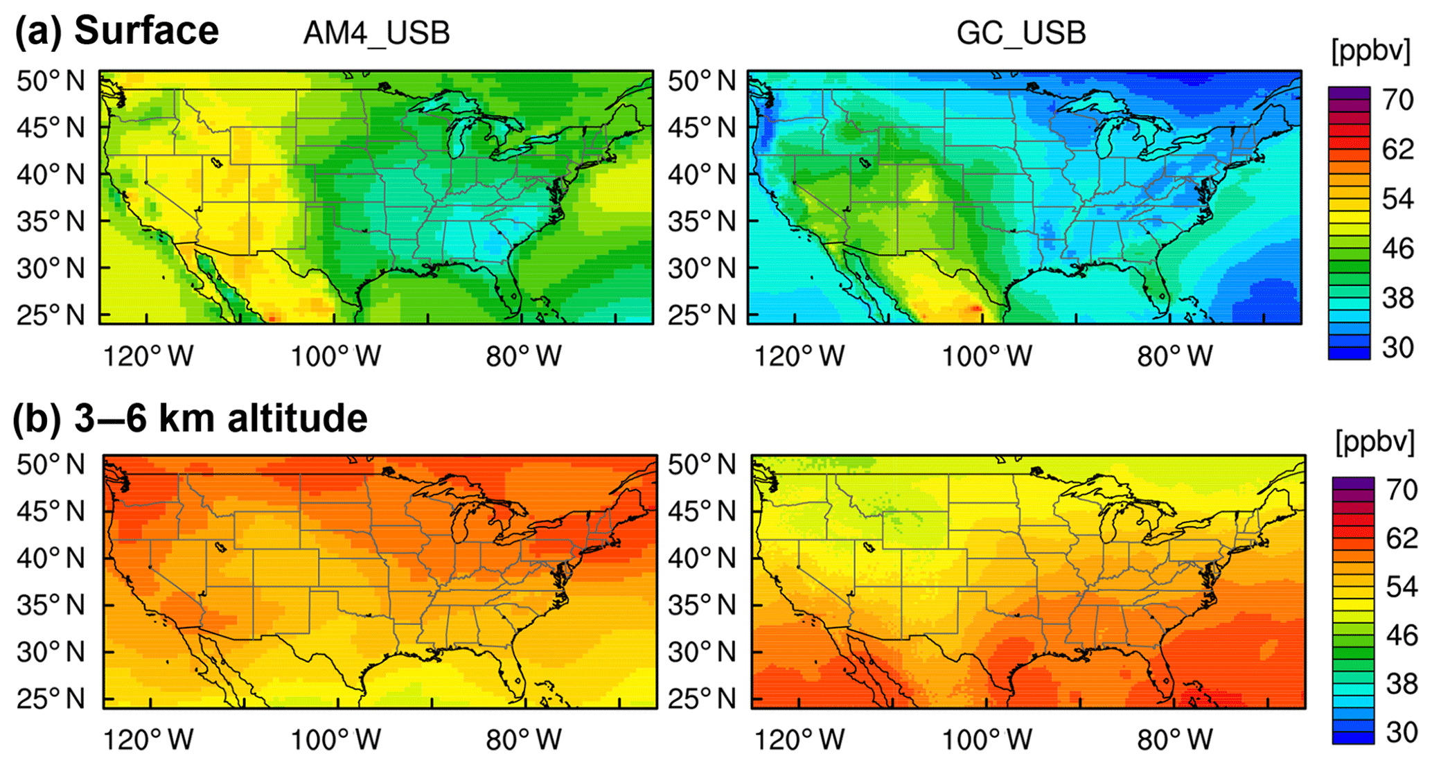
Figure 16Spatial distributions of USB O3 simulated with GFDL-AM4 and GEOS-Chem (a) at the surface (MDA8) and (b) at 3–6 km altitude (24 h mean) during April–June 2017.
Through a process-oriented analysis of intensive measurements from the 2017 FAST-LVOS field campaign and high-resolution simulations with two global models (GFDL-AM4 and GEOS-Chem), we study the sources of observed MDA8 O3 above 65 ppbv in the SWUS. The attribution of each event to a specific source is sometimes challenging, despite an integrated analysis of multi-tracer, multi-platform observations and model simulations. We identify the high-O3 events associated with stratospheric intrusions (22–23 April, 13–14 May, and 11–13 June), the mixing of local pollution and transported stratospheric O3 (14 June), regional or local anthropogenic pollution (2, 16, and 29–30 June), wildfires (22 June), and the mixing of Asian pollution with regional pollution (24 May). We also discuss an event (28 June) likely resulting from the fine-scale transport of fire plumes or pollution from southern California, although a solid attribution for this event is challenging based on available data.
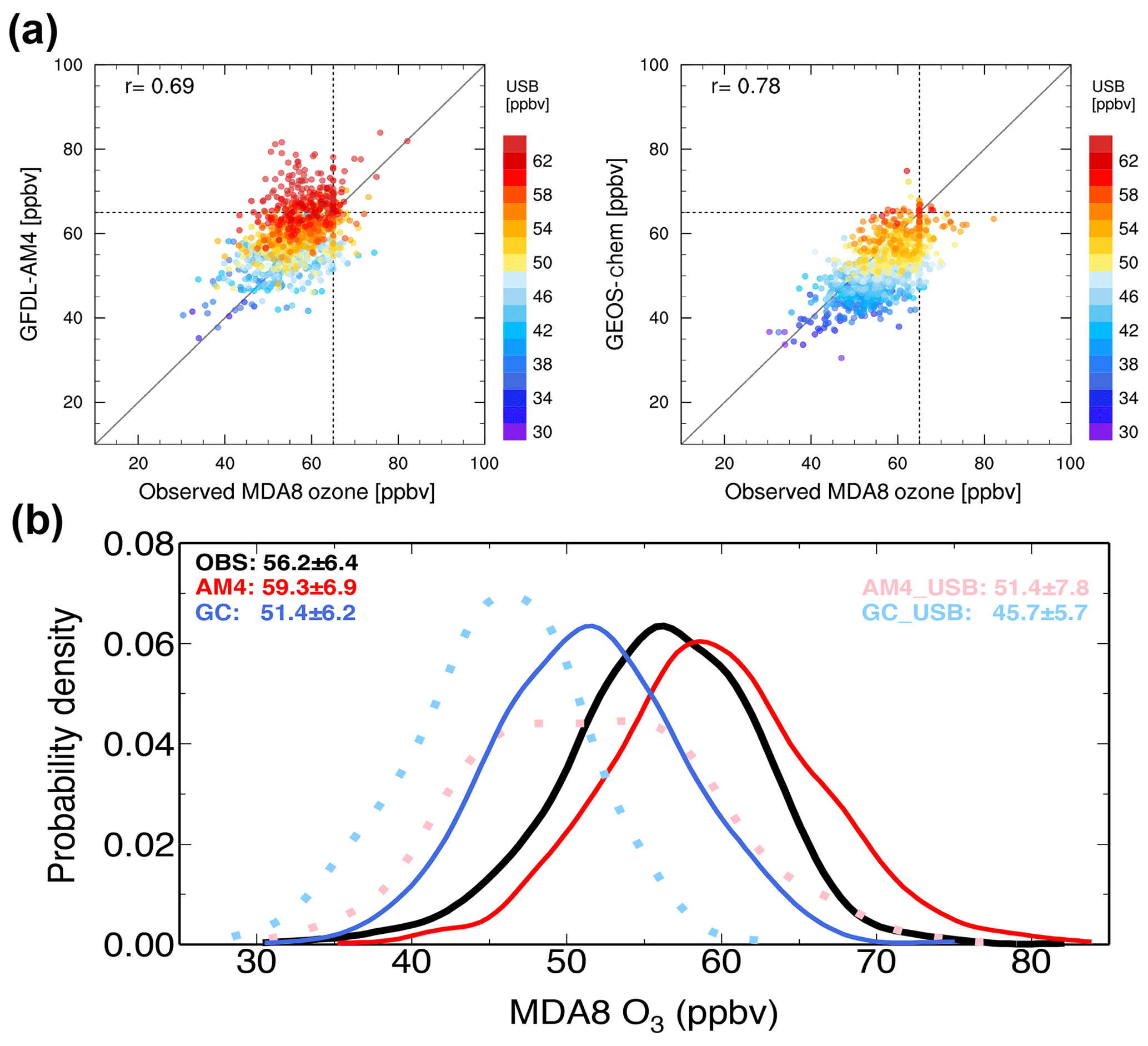
Figure 17(a) Scatterplots of observed versus simulated daily MDA8 O3, color-coded by USB O3, at 12 WUS high-elevation sites (circles in Fig. 1a) during April–June 2017. The dashed lines mark the 65 ppbv threshold. (b) Probability density of daily MDA8 O3 as observed (solid black) and simulated with GFDL-AM4 (solid red) and GEOS-Chem (solid blue), along with the distribution of USB O3 estimated from each model (dotted lines).
During the 11–13 June deep stratospheric intrusion event, the NOAA mobile lab measurements at Angel Peak show a sharp increase in O3 coinciding with a decrease in CO and water vapor, a marker for air of stratospheric origin. These characteristics are in contrast to the concurrent increases in O3 and CO in humid, warm urban plumes and wildfire plumes transported from the Las Vegas Valley. The observed relationships can provide a useful first indication of high-O3 events influenced directly by a deep intrusion. However, once transported stratospheric O3 is mixed into regional pollution, model diagnostic tracers are needed to quantify the stratospheric impact. For instance, on 14 June, observations at Angel Peak show positive O3∕CO correlations, while O3Strat in GFDL-AM4 shows 20–30 ppbv enhancements above its mean level at Angel Peak and at surface sites across the SWUS where the observed and simulated total MDA8 O3 concentrations were above 70 ppbv. These quantitative model attributions are only as good as the precision and capability of the models.
GFDL-AM4 and GEOS-Chem differ significantly in simulating stratosphere-to-troposphere transport events, affecting their ability to simulate USB mean levels and extreme events. During the 11–14 June STT event, GFDL-AM4 captures the key characteristics of deep stratospheric intrusions, consistent with lidar profiles and ozonesondes, whereas GEOS-Chem with simplified stratospheric chemistry and dynamics has difficulty simulating the observed features. At the surface, on days when observed MDA8 O3 exceeds 65 ppbv and AM4 O3Strat is 20–40 ppbv above its mean baseline level, AM4 simulates 15–20 ppbv greater USB O3 than GEOS-Chem (Figs. 4 and 9). During these STT events, total MDA8 O3 abundances simulated by the two models often bracket the observed values, as noted previously by Fiore et al. (2014). The FAST-LVOS analysis, combined with our earlier multi-year studies (Lin et al. 2012a, 2015a), indicates that GFDL AM3/AM4 with nudged meteorology captures the timing and locations of the observed O3 enhancements in surface air and aloft during STT events and is thus useful for the screening of exceptional events due to STT. AM3/AM4 typically spreads the STT enhancement across a wider range of sites over the southwest rather than capturing the observed localized feature, causing high biases of total MDA8 O3 during some STT events (Lin et al., 2012a). Thus, we propose targeted analysis of the observed high-O3 events, rather than the modeled events, and recommend bias correction to simulated USB O3 in AM4, such as the approach used by Lin et al. (2012a). For the future application of GEOS-Chem for USB estimates, we recommend the version with the Universal tropospheric-stratospheric Chemistry eXtension (UCX) mechanism (Eastham et al., 2014) and process-oriented evaluation using daily ozonesondes and lidar profiles.
The two models also differ substantially in total and background O3 simulations during the 22 June wildfire event. GEOS-Chem captures the broad O3 enhancement in lidar observations but overestimates surface MDA8 O3 at some sites during this event. It remains unclear whether the higher USB O3 simulated by GEOS-Chem during this event is from greater O3 produced from wildfire emissions or excessive lightning NOx emissions in the model. Although GFDL-AM3 captures the observed interannual variability in O3 enhancements from large-scale wildfires over the WUS (Lin et al., 2017), GFDL-AM4 has difficulty simulating the observed O3 enhancements during the relatively small-scale wildfire event on 22 June. Sensitivity simulations with fire emissions constrained at the surface or with part of fire NOx emissions emitted as PAN and HNO3 do not substantially improve simulated O3 on 22 June. Wildfires typically occur under hot, dry conditions, which also enable the buildup of O3 produced from regional anthropogenic emissions, complicating an unambiguous attribution of the high-O3 events solely based on observations. Screening of exceptional events due to wildfire emissions remains a serious challenge.
The multi-model approach tied closely to intensive measurements provides insights into the capability of models to simulate background O3 and harnesses the strengths of individual models to characterize the sources of high-O3 events. Stratospheric intrusions, Asian pollution, and wildfires are important sources of the observed high-O3 events above 65 ppbv in the SWUS, although uncertainties remain in the quantitative attribution. These uncertainties may lie not only in O3 sources but also in O3 sinks, such as removal by vegetation (e.g., Lin et al., 2019, 2020). Surface ozone in China continues to increase despite regional NOx emission controls in recent years (Liu et al., 2016; Li et al., 2019; Sun et al., 2016). Furthermore, the increasing frequency of wildfires under a warming climate (e.g., Westerling et al., 2006; Dennison et al., 2014) and growing global methane levels (e.g., West et al., 2006; Morgenstern et al., 2013) may foster higher background O3 levels in the coming decades (Lin et al., 2017). These increasing background O3 sources, together with year-to-year variability in stratospheric influence (Lin et al., 2015a), will leave little margin for O3 produced from local and regional emissions, posing challenges to achieving a potentially tightened O3 NAAQS in the SWUS.
Model simulations presented in this paper are available upon request to the corresponding author (alex.zhang@noaa.gov). Field measurements during FAST-LVOS are available at https://www.esrl.noaa.gov/csd/projects/fastlvos (last access: 3 July 2019; NOAA, 2019).
The supplement related to this article is available online at: https://doi.org/10.5194/acp-20-10379-2020-supplement.
ML conceived this study and designed the model experiments; LZ performed the GFDL-AM4 simulations and all analysis under the supervision of ML; EK and YW conducted the GEOS-Chem simulations; LWH and YW assisted in the interpretation of model results; AOL, CJS, RJA, IP, PC, JP, TBR, SSB, ZCJD, GK, and SC carried out field measurements. LZ and ML wrote the article with inputs from all coauthors.
The authors declare that they have no conflict of interest.
The statements, findings, and conclusions are those of the author(s) and should not be construed as the views of the agencies.
We are grateful to Zheng Li (Clark County Department of Air Quality), Songmiao Fan (GFDL), and Yuanyu Xie (Princeton University) for helpful discussions and suggestions. We thank Qiang Zhang (Tsinghua University) for providing trends of anthropogenic NOx emissions in China and Christine Wiedinmyer (University of Colorado) for the 2017 FINN emission data.
This research has been supported by the Clark County Department of Air Quality (grant nos. CBE 604279-16, CBE 604318-16, and CBE 604380-17) and the Cooperative Institute for Modeling the Earth System (CIMES) between NOAA and Princeton University (grant nos. NA14OAR4320106 and NA18OAR4320123).
This paper was edited by Jason West and reviewed by two anonymous referees.
Akritidis, D., Katragkou, E., Zanis, P., Pytharoulis, I., Melas, D., Flemming, J., Inness, A., Clark, H., Plu, M., and Eskes, H.: A deep stratosphere-to-troposphere ozone transport event over Europe simulated in CAMS global and regional forecast systems: analysis and evaluation, Atmos. Chem. Phys., 18, 15515–15534, https://doi.org/10.5194/acp-18-15515-2018, 2018.
Alvarado, M. J., Logan, J. A., Mao, J., Apel, E., Riemer, D., Blake, D., Cohen, R. C., Min, K.-E., Perring, A. E., Browne, E. C., Wooldridge, P. J., Diskin, G. S., Sachse, G. W., Fuelberg, H., Sessions, W. R., Harrigan, D. L., Huey, G., Liao, J., Case-Hanks, A., Jimenez, J. L., Cubison, M. J., Vay, S. A., Weinheimer, A. J., Knapp, D. J., Montzka, D. D., Flocke, F. M., Pollack, I. B., Wennberg, P. O., Kurten, A., Crounse, J., Clair, J. M. St., Wisthaler, A., Mikoviny, T., Yantosca, R. M., Carouge, C. C., and Le Sager, P.: Nitrogen oxides and PAN in plumes from boreal fires during ARCTAS-B and their impact on ozone: an integrated analysis of aircraft and satellite observations, Atmos. Chem. Phys., 10, 9739–9760, https://doi.org/10.5194/acp-10-9739-2010, 2010.
Alvarez II, R. J., Senff, C. J., Langford, A. O., Weickmann, A. M., Law, D. C., Machol, J. L., Merritt, D. A., Marchbanks, R. D., Sandberg, S. P., Brewer, W. A., Hardesty, R. M., and Banta, R. M.: Development and Application of a Compact, Tunable, Solid-State Airborne Ozone Lidar System for Boundary Layer Profiling, J. Atmos. Ocean. Technol., 28, 1258–1272, https://doi.org/10.1175/jtech-d-10-05044.1, 2011.
Barletta, B., Meinardi, S., Simpson, I. J., Atlas, E. L., Beyersdorf, A. J., Baker, A. K., Blake, N. J., Yang, M., Midyett, J. R., Novak, B. J., McKeachie, R. J., Fuelberg, H. E., Sachse, G. W., Avery, M. A., Campos, T., Weinheimer, A. J., Rowland, F. S., and Blake, D. R.: Characterization of volatile organic compounds (VOCs) in Asian and north American pollution plumes during INTEX-B: identification of specific Chinese air mass tracers, Atmos. Chem. Phys., 9, 5371–5388, https://doi.org/10.5194/acp-9-5371-2009, 2009.
Baylon, P. M., Jaffe, D. A., Pierce, R. B., and Gustin, M. S.: Interannual Variability in Baseline Ozone and Its Relationship to Surface Ozone in the Western U.S, Environ. Sci. Technol., 50, 2994–3001, https://doi.org/10.1021/acs.est.6b00219, 2016.
Bey, I., Jacob, D. J., Yantosca, R. M., Logan, J. A., Field, B. D., Fiore, A. M., Li, Q., Liu, H. Y., Mickley, L. J., and Schultz, M. G.: Global modeling of tropospheric chemistry with assimilated meteorology: Model description and evaluation, J. Geophys. Res.-Atmos., 106, 23073–23095, https://doi.org/10.1029/2001JD000807, 2001.
Bonin, T. A., Carroll, B. J., Hardesty, R. M., Brewer, W. A., Hajny, K., Salmon, O. E., and Shepson, P. B.: Doppler Lidar Observations of the Mixing Height in Indianapolis Using an Automated Composite Fuzzy Logic Approach, J. Atmos. Ocean. Technol., 35, 473–490, https://doi.org/10.1175/jtech-d-17-0159.1, 2018.
Chen, D., Wang, Y., McElroy, M. B., He, K., Yantosca, R. M., and Le Sager, P.: Regional CO pollution and export in China simulated by the high-resolution nested-grid GEOS-Chem model, Atmos. Chem. Phys., 9, 3825–3839, https://doi.org/10.5194/acp-9-3825-2009, 2009.
Cooper, O., Forster, C., Parrish, D., Dunlea, E., Hübler, G., Fehsenfeld, F., Holloway, J., Oltmans, S., Johnson, B., Wimmers, A., and Horowitz, L.: On the life cycle of a stratospheric intrusion and its dispersion into polluted warm conveyor belts, J. Geophys. Res.-Atmos., 109, D23S09, https://doi.org/10.1029/2003JD004006, 2004.
Dennison, P. E., Brewer, S. C., Arnold, J. D., and Moritz, M. A.: Large wildfire trends in the western United States, 1984–2011, Geophys. Res. Lett., 41, 2928–2933, https://doi.org/10.1002/2014gl059576, 2014.
Dentener, F., Kinne, S., Bond, T., Boucher, O., Cofala, J., Generoso, S., Ginoux, P., Gong, S., Hoelzemann, J. J., Ito, A., Marelli, L., Penner, J. E., Putaud, J.-P., Textor, C., Schulz, M., van der Werf, G. R., and Wilson, J.: Emissions of primary aerosol and precursor gases in the years 2000 and 1750 prescribed data-sets for AeroCom, Atmos. Chem. Phys., 6, 4321–4344, https://doi.org/10.5194/acp-6-4321-2006, 2006.
Dolwick, P., Akhtar, F., Baker, K. R., Possiel, N., Simon, H., and Tonnesen, G.: Comparison of background ozone estimates over the western United States based on two separate model methodologies, Atmos. Environ., 109, 282–296, https://doi.org/10.1016/j.atmosenv.2015.01.005, 2015.
Donner, L. J., Wyman, B. L., Hemler, R. S., Horowitz, L. W., Ming, Y., Zhao, M., Golaz, J.-C., Ginoux, P., Lin, S.-J., Schwarzkopf, M. D., Austin, J., Alaka, G., Cooke, W. F., Delworth, T. L., Freidenreich, S. M., Gordon, C. T., Griffies, S. M., Held, I. M., Hurlin, W. J., Klein, S. A., Knutson, T. R., Langenhorst, A. R., Lee, H.-C., Lin, Y., Magi, B. I., Malyshev, S. L., Milly, P. C. D., Naik, V., Nath, M. J., Pincus, R., Ploshay, J. J., Ramaswamy, V., Seman, C. J., Shevliakova, E., Sirutis, J. J., Stern, W. F., Stouffer, R. J., Wilson, R. J., Winton, M., Wittenberg, A. T., and Zeng, F.: The Dynamical Core, Physical Parameterizations, and Basic Simulation Characteristics of the Atmospheric Component AM3 of the GFDL Global Coupled Model CM3, J. Climate, 24, 3484–3519, https://doi.org/10.1175/2011jcli3955.1, 2011.
Eastham, S. D., Weisenstein, D. K., and Barrett, S. R. H.: Development and evaluation of the unified tropospheric–stratospheric chemistry extension (UCX) for the global chemistry-transport model GEOS-Chem, Atmos. Environ., 89, 52–63, https://doi.org/10.1016/j.atmosenv.2014.02.001, 2014.
Emery, C., Jung, J., Downey, N., Johnson, J., Jimenez, M., Yarwood, G., and Morris, R.: Regional and global modeling estimates of policy relevant background ozone over the United States, Atmos. Environ., 47, 206–217, https://doi.org/10.1016/j.atmosenv.2011.11.012, 2012.
Faloona, I. C., Chiao, S., Eiserloh, A. J., II, R. J. A., Kirgis, G., Langford, A. O., Senff, C. J., Caputi, D., Hu, A., Iraci, L. T., Yates, E. L., Marrero, J. E., Ryoo, J.-M., Conley, S., Tanrikulu, S., Xu, J., and Kuwayama, T.: The California Baseline Ozone Transport Study (CABOTS), B. Am. Meteor. Soc., 101, E427–E445, https://doi.org/10.1175/bams-d-18-0302.1, 2020.
Fiore, A. M., Oberman, J. T., Lin, M. Y., Zhang, L., Clifton, O. E., Jacob, D. J., Naik, V., Horowitz, L. W., Pinto, J. P., and Milly, G. P.: Estimating North American background ozone in U.S. surface air with two independent global models: Variability, uncertainties, and recommendations, Atmos. Environ., 96, 284–300, https://doi.org/10.1016/j.atmosenv.2014.07.045, 2014.
Gong, X., Kaulfus, A., Nair, U., and Jaffe, D. A.: Quantifying O3 Impacts in Urban Areas Due to Wildfires Using a Generalized Additive Model, Environ. Sci. Technol., 51, 13216–13223, https://doi.org/10.1021/acs.est.7b03130, 2017.
Guenther, A., Karl, T., Harley, P., Wiedinmyer, C., Palmer, P. I., and Geron, C.: Estimates of global terrestrial isoprene emissions using MEGAN (Model of Emissions of Gases and Aerosols from Nature), Atmos. Chem. Phys., 6, 3181–3210, https://doi.org/10.5194/acp-6-3181-2006, 2006.
Guo, J. J., Fiore, A. M., Murray, L. T., Jaffe, D. A., Schnell, J. L., Moore, C. T., and Milly, G. P.: Average versus high surface ozone levels over the continental USA: model bias, background influences, and interannual variability, Atmos. Chem. Phys., 18, 12123–12140, https://doi.org/10.5194/acp-18-12123-2018, 2018.
Herman, R. L., Webster, C. R., May, R. D., Scott, D. C., Hu, H., Moyer, E. J., Wennberg, P. O., Hanisco, T. F., Lanzendorf, E. J., Salawitch, R. J., Yung, Y. L., Margitan, J. J., and Bui, T. P.: Measurements of CO in the upper troposphere and lower stratosphere, Chemosphere – Global Change Sci., 1, 173–183, https://doi.org/10.1016/S1465-9972(99)00008-2, 1999.
Hoesly, R. M., Smith, S. J., Feng, L., Klimont, Z., Janssens-Maenhout, G., Pitkanen, T., Seibert, J. J., Vu, L., Andres, R. J., Bolt, R. M., Bond, T. C., Dawidowski, L., Kholod, N., Kurokawa, J.-I., Li, M., Liu, L., Lu, Z., Moura, M. C. P., O'Rourke, P. R., and Zhang, Q.: Historical (1750–2014) anthropogenic emissions of reactive gases and aerosols from the Community Emissions Data System (CEDS), Geosci. Model Dev., 11, 369–408, https://doi.org/10.5194/gmd-11-369-2018, 2018.
Holzinger, R., Warneke, C., Hansel, A., Jordan, A., Lindinger, W., Scharffe, D. H., Schade, G., and Crutzen, P. J.: Biomass burning as a source of formaldehyde, acetaldehyde, methanol, acetone, acetonitrile, and hydrogen cyanide, Geophys. Res. Lett., 26, 1161–1164, https://doi.org/10.1029/1999gl900156, 1999.
Horowitz, L. W., Naik, V., Paulot, F., Ginoux, P. A., Dunne, J. P.,, Mao, J., Schnell, J., Chen, X., He, J., Lin, M., Lin, P., Malyshev,, and S., P., D., Shevliakova, E., and Zhao, M.: The GFDL Global Atmospheric Chemistry-Climate Model AM4.1: Model Description and Simulation Characteristics, J. Adv. Model. Earth Syst., https://doi.org/10.1029/2019MS002032, in press, 2020.
Jacob, D. J., Logan, J. A., and Murti, P. P.: Effect of rising Asian emissions on surface ozone in the United States, Geophys. Res. Lett., 26, 2175–2178, https://doi.org/10.1029/1999GL900450, 1999.
Jaffe, D. A. and Wigder, N. L.: Ozone production from wildfires: A critical review, Atmos. Environ., 51, 1–10, https://doi.org/10.1016/j.atmosenv.2011.11.063, 2012.
Jaffe, D. A., Wigder, N., Downey, N., Pfister, G., Boynard, A., and Reid, S. B.: Impact of Wildfires on Ozone Exceptional Events in the Western U.S, Environ. Sci. Technol., 47, 11065–11072, https://doi.org/10.1021/es402164f, 2013.
Jaffe, D. A., Cooper, O. R., Fiore, A. M., Henderson, B. H., Tonneson, G. S., Russell, A. G., Henze, D. K., Langford, A. O., Lin, M., and Moore, T.: Scientific assessment of background ozone over the U.S.: Implications for air quality management, Elementa: Sci. Anthropo., 6, 1–30, https://doi.org/10.1525/elementa.309, 2018.
Langford, A. O., Aikin, K. C., Eubank, C. S., and Williams, E. J.: Stratospheric contribution to high surface ozone in Colorado during springtime, Geophys. Res. Lett., 36, L12801, https://doi.org/10.1029/2009GL038367, 2009.
Langford, A. O., Senff, C. J., Alvarez, R. J., Banta, R. M., and Hardesty, R. M.: Long-range transport of ozone from the Los Angeles Basin: A case study, Geophys. Res. Lett., 37, L06807, https://doi.org/10.1029/2010GL042507, 2010.
Langford, A. O., Brioude, J., Cooper, O. R., Senff, C. J., Alvarez, R. J., Hardesty, R. M., Johnson, B. J., and Oltmans, S. J.: Stratospheric influence on surface ozone in the Los Angeles area during late spring and early summer of 2010, J. Geophys. Res.-Atmos., 117, D00V06, https://doi.org/10.1029/2011JD016766, 2012.
Langford, A. O., Senff, C. J., Alvarez, R. J., Brioude, J., Cooper, O. R., Holloway, J. S., Lin, M. Y., Marchbanks, R. D., Pierce, R. B., Sandberg, S. P., Weickmann, A. M., and Williams, E. J.: An overview of the 2013 Las Vegas Ozone Study (LVOS): Impact of stratospheric intrusions and long-range transport on surface air quality, Atmos. Environ., 109, 305–322, https://doi.org/10.1016/j.atmosenv.2014.08.040, 2015.
Langford, A. O., Alvarez II, R. J., Brioude, J., Fine, R., Gustin, M. S., Lin, M. Y., Marchbanks, R. D., Pierce, R. B., Sandberg, S. P., Senff, C. J., Weickmann, A. M., and Williams, E. J.: Entrainment of stratospheric air and Asian pollution by the convective boundary layer in the southwestern U.S, J. Geophys. Res.-Atmos., 122, 1312–1337, https://doi.org/10.1002/2016JD025987, 2017.
Langford, A. O., Alvarez II, R. J., Kirgis, G., Senff, C. J., Caputi, D., Conley, S. A., Faloona, I. C., Iraci, L. T., Marrero, J. E., McNamara, M. E., Ryoo, J.-M., and Yates, E. L.: Intercomparison of lidar, aircraft, and surface ozone measurements in the San Joaquin Valley during the California Baseline Ozone Transport Study (CABOTS), Atmos. Meas. Tech., 12, 1889–1904, https://doi.org/10.5194/amt-12-1889-2019, 2019.
Langford, A. O., Aikin, K. C., Alvarez II, R. J., Ahmadov, R., Baidar, S., Bonin, T. A., Brewer, A. W., Brioude, J., Brown, S. S., Caputi, D. J., Conley, S. A., Cullis, P. D., Decker, Z., Evan, S., Kirgis, G., Lin, M., Pagowski, M., Peischl, J., Petropavlovskikh, I., Pierce, R. B., Ryerson, T. B., Sandberg, S. P., Senff, C. J., Sterling, C. W., Weickmann, A. M., and Zhang, L.: The Fires, Asian, and Stratospheric Transport-Las Vegas Ozone Study (FAST-LVOS), in preparation, 2020.
Li, J., Mao, J., Min, K.-E., Washenfelder, R. A., Brown, S. S., Kaiser, J., Keutsch, F. N., Volkamer, R., Wolfe, G. M., Hanisco, T. F., Pollack, I. B., Ryerson, T. B., Graus, M., Gilman, J. B., Lerner, B. M., Warneke, C., de Gouw, J. A., Middlebrook, A. M., Liao, J., Welti, A., Henderson, B. H., McNeill, V. F., Hall, S. R., Ullmann, K., Donner, L. J., Paulot, F., and Horowitz, L. W.: Observational constraints on glyoxal production from isoprene oxidation and its contribution to organic aerosol over the Southeast United States, J. Geophys. Res.-Atmos., 121, 9849–9861, https://doi.org/10.1002/2016jd025331, 2016.
Li, K., Jacob, D. J., Liao, H., Shen, L., Zhang, Q., and Bates, K. H.: Anthropogenic drivers of 2013–2017 trends in summer surface ozone in China, P. Natl. Acad. Sci. USA, 116, 422–427, https://doi.org/10.1073/pnas.1812168116, 2019.
Li, M., Zhang, Q., Kurokawa, J.-I., Woo, J.-H., He, K., Lu, Z., Ohara, T., Song, Y., Streets, D. G., Carmichael, G. R., Cheng, Y., Hong, C., Huo, H., Jiang, X., Kang, S., Liu, F., Su, H., and Zheng, B.: MIX: a mosaic Asian anthropogenic emission inventory under the international collaboration framework of the MICS-Asia and HTAP, Atmos. Chem. Phys., 17, 935–963, https://doi.org/10.5194/acp-17-935-2017, 2017.
Lin, M., Fiore, A. M., Cooper, O. R., Horowitz, L. W., Langford, A. O., Levy II, H., Johnson, B. J., Naik, V., Oltmans, S. J., and Senff, C. J.: Springtime high surface ozone events over the western United States: Quantifying the role of stratospheric intrusions, J. Geophys. Res.-Atmos., 117, D00V22, https://doi.org/10.1029/2012JD018151, 2012a.
Lin, M., Fiore, A. M., Horowitz, L. W., Cooper, O. R., Naik, V., Holloway, J., Johnson, B. J., Middlebrook, A. M., Oltmans, S. J., Pollack, I. B., Ryerson, T. B., Warner, J. X., Wiedinmyer, C., Wilson, J., and Wyman, B.: Transport of Asian ozone pollution into surface air over the western United States in spring, J. Geophys. Res.-Atmos., 117, D00V07, https://doi.org/10.1029/2011JD016961, 2012b.
Lin, M., Fiore, A. M., Horowitz, L. W., Langford, A. O., Oltmans, S. J., Tarasick, D., and Rieder, H. E.: Climate variability modulates western US ozone air quality in spring via deep stratospheric intrusions, Nat. Commun., 6, 7105, https://doi.org/10.1038/ncomms8105, 2015a.
Lin, M., Horowitz, L. W., Cooper, O. R., Tarasick, D., Conley, S., Iraci, L. T., Johnson, B., Leblanc, T., Petropavlovskikh, I., and Yates, E. L.: Revisiting the evidence of increasing springtime ozone mixing ratios in the free troposphere over western North America, Geophys. Res. Lett., 42, 8719–8728, https://doi.org/10.1002/2015GL065311, 2015b.
Lin, M., Horowitz, L. W., Payton, R., Fiore, A. M., and Tonnesen, G.: US surface ozone trends and extremes from 1980 to 2014: quantifying the roles of rising Asian emissions, domestic controls, wildfires, and climate, Atmos. Chem. Phys., 17, 2943–2970, https://doi.org/10.5194/acp-17-2943-2017, 2017.
Lin, M., Malyshev, S., Shevliakova, E., Paulot, F., Horowitz, L. W., Fares, S., Mikkelsen, T. N., and Zhang, L.: Sensitivity of ozone dry deposition to ecosystem-atmosphere interactions: A critical appraisal of observations and simulations, Global Biogeochem. Cy., 30, 1264–1288, https://doi.org/10.1029/2018gb006157, 2019.
Lin, M., Horowitz, L. W., Xie, Y., Paulot, F., Malyshev, S., Shevliakova, E., Finco, A., Gerosa, G., Kubistin, D., and Pilegaard, K.: Vegetation feedbacks during drought exacerbate ozone air pollution extremes in Europe, Nat. Clim. Chang. 10, 444–451, https://doi.org/10.1038/s41558-020-0743-y, 2020.
Liu, F., Zhang, Q., van der A, R. J., Zheng, B., Tong, D., Yan, L., Zheng, Y., and He, K.: Recent reduction in NO x emissions over China: synthesis of satellite observations and emission inventories, Environ. Res. Lett., 11, 114002, https://doi.org/10.1088/1748-9326/11/11/114002, 2016.
Mao, J., Horowitz, L. W., Naik, V., Fan, S., Liu, J., and Fiore, A. M.: Sensitivity of tropospheric oxidants to biomass burning emissions: implications for radiative forcing, Geophys. Res. Lett., 40, 1241–1246, https://doi.org/10.1002/grl.50210, 2013a.
Mao, J., Paulot, F., Jacob, D. J., Cohen, R. C., Crounse, J. D., Wennberg, P. O., Keller, C. A., Hudman, R. C., Barkley, M. P., and Horowitz, L. W.: Ozone and organic nitrates over the eastern United States: Sensitivity to isoprene chemistry, J. Geophys. Res.-Atmos., 118, 11256–211268, https://doi.org/10.1002/jgrd.50817, 2013b.
McLinden, C. A., Olsen, S. C., Hannegan, B., Wild, O., Prather, M. J., and Sundet, J.: Stratospheric ozone in 3-D models: A simple chemistry and the cross-tropopause flux, J. Geophys. Res.-Atmos., 105, 14653–14665, https://doi.org/10.1029/2000jd900124, 2000.
Morgenstern, O., Zeng, G., Luke Abraham, N., Telford, P. J., Braesicke, P., Pyle, J. A., Hardiman, S. C., O'Connor, F. M., and Johnson, C. E.: Impacts of climate change, ozone recovery, and increasing methane on surface ozone and the tropospheric oxidizing capacity, J. Geophys. Res.-Atmos., 118, 1028–1041, https://doi.org/10.1029/2012jd018382, 2013.
Murray, L. T., Jacob, D. J., Logan, J. A., Hudman, R. C., and Koshak, W. J.: Optimized regional and interannual variability of lightning in a global chemical transport model constrained by LIS/OTD satellite data, J. Geophys. Res.-Atmos., 117, D20307, https://doi.org/10.1029/2012jd017934, 2012.
Naik, V., Horowitz, L. W., Fiore, A. M., Ginoux, P., Mao, J., Aghedo, A. M., and Levy II, H.: Impact of preindustrial to present-day changes in short-lived pollutant emissions on atmospheric composition and climate forcing, J. Geophys. Res.-Atmos., 118, 8086–8110, https://doi.org/10.1002/jgrd.50608, 2013.
NOAA: Fires, Asian, and Stratospheric Transport – Las Vegas Ozone Study (FAST-LVOS), available at: https://www.esrl.noaa.gov/csd/projects/fastlvos, last access: 3 July 2019.
Parrish, D. D., Trainer, M., Holloway, J. S., Yee, J. E., Warshawsky, M. S., Fehsenfeld, F. C., Forbes, G. L., and Moody, J. L.: Relationships between ozone and carbon monoxide at surface sites in the North Atlantic region, J. Geophys. Res.-Atmos., 103, 13357–13376, https://doi.org/10.1029/98JD00376, 1998.
Paulot, F., Ginoux, P., Cooke, W. F., Donner, L. J., Fan, S., Lin, M.-Y., Mao, J., Naik, V., and Horowitz, L. W.: Sensitivity of nitrate aerosols to ammonia emissions and to nitrate chemistry: implications for present and future nitrate optical depth, Atmos. Chem. Phys., 16, 1459–1477, https://doi.org/10.5194/acp-16-1459-2016, 2016.
Paulot, F., Paynter, D., Ginoux, P., Naik, V., Whitburn, S., Van Damme, M., Clarisse, L., Coheur, P.-F., and Horowitz, L. W.: Gas-aerosol partitioning of ammonia in biomass burning plumes: Implications for the interpretation of spaceborne observations of ammonia and the radiative forcing of ammonium nitrate, Geophys. Res. Lett., 44, 8084–8093, https://doi.org/10.1002/2017GL074215, 2017.
Prather, M. J., Zhu, X., Tang, Q., Hsu, J., and Neu, J. L.: An atmospheric chemist in search of the tropopause, J. Geophys. Res.-Atmos., 116, D04306, https://doi.org/10.1029/2010JD014939, 2011.
Rasmussen, D. J., Fiore, A. M., Naik, V., Horowitz, L. W., McGinnis, S. J., and Schultz, M. G.: Surface ozone–temperature relationships in the eastern US: a monthly climatology for evaluating chemistry–climate models, Atmos. Environ., 47, 142–153, https://doi.org/10.1016/j.atmosenv.2011.11.021, 2012.
Schnell, J. L., Naik, V., Horowitz, L. W., Paulot, F., Mao, J., Ginoux, P., Zhao, M., and Ram, K.: Exploring the relationship between surface PM2.5 and meteorology in Northern India, Atmos. Chem. Phys., 18, 10157–10175, https://doi.org/10.5194/acp-18-10157-2018, 2018.
Singh, H. B., Cai, C., Kaduwela, A., Weinheimer, A., and Wisthaler, A.: Interactions of fire emissions and urban pollution over California: Ozone formation and air quality simulations, Atmos. Environ., 56, 45–51, https://doi.org/10.1016/j.atmosenv.2012.03.046, 2012.
Sun, L., Xue, L., Wang, T., Gao, J., Ding, A., Cooper, O. R., Lin, M., Xu, P., Wang, Z., Wang, X., Wen, L., Zhu, Y., Chen, T., Yang, L., Wang, Y., Chen, J., and Wang, W.: Significant increase of summertime ozone at Mount Tai in Central Eastern China, Atmos. Chem. Phys., 16, 10637–10650, https://doi.org/10.5194/acp-16-10637-2016, 2016.
Travis, K. R., Jacob, D. J., Fisher, J. A., Kim, P. S., Marais, E. A., Zhu, L., Yu, K., Miller, C. C., Yantosca, R. M., Sulprizio, M. P., Thompson, A. M., Wennberg, P. O., Crounse, J. D., St. Clair, J. M., Cohen, R. C., Laughner, J. L., Dibb, J. E., Hall, S. R., Ullmann, K., Wolfe, G. M., Pollack, I. B., Peischl, J., Neuman, J. A., and Zhou, X.: Why do models overestimate surface ozone in the Southeast United States?, Atmos. Chem. Phys., 16, 13561–13577, https://doi.org/10.5194/acp-16-13561-2016, 2016.
Trickl, T., Vogelmann, H., Fix, A., Schäfler, A., Wirth, M., Calpini, B., Levrat, G., Romanens, G., Apituley, A., Wilson, K. M., Begbie, R., Reichardt, J., Vömel, H., and Sprenger, M.: How stratospheric are deep stratospheric intrusions? LUAMI 2008, Atmos. Chem. Phys., 16, 8791–8815, https://doi.org/10.5194/acp-16-8791-2016, 2016.
U.S. Environmental Protection Agency: Treatment of data influenced by exceptional events, edited by U. S. Environmental Protection Agency, Research Triangle Park, North Carolina, United States of America, 68216–68282, 2016.
Wang, Y. X., McElroy, M. B., Jacob, D. J., and Yantosca, R. M.: A nested grid formulation for chemical transport over Asia: Applications to CO, J. Geophys. Res.-Atmos., 109, D22307, https://doi.org/10.1029/2004JD005237, 2004.
West, J. J., Fiore, A. M., Horowitz, L. W., and Mauzerall, D. L.: Global health benefits of mitigating ozone pollution with methane emission controls, P. Natl. Acad. Sci. USA, 103, 3988–3993, https://doi.org/10.1073/pnas.0600201103, 2006.
Westerling, A. L., Hidalgo, H. G., Cayan, D. R., and Swetnam, T. W.: Warming and Earlier Spring Increase Western U.S. Forest Wildfire Activity, Science, 313, 940–943, https://doi.org/10.1126/science.1128834, 2006.
Wiedinmyer, C., Akagi, S. K., Yokelson, R. J., Emmons, L. K., Al-Saadi, J. A., Orlando, J. J., and Soja, A. J.: The Fire INventory from NCAR (FINN): a high resolution global model to estimate the emissions from open burning, Geosci. Model Dev., 4, 625–641, https://doi.org/10.5194/gmd-4-625-2011, 2011.
Wild, R. J., Dubé, W. P., Aikin, K. C., Eilerman, S. J., Neuman, J. A., Peischl, J., Ryerson, T. B., and Brown, S. S.: On-road measurements of vehicle NO2∕NOx emission ratios in Denver, Colorado, USA, Atmos. Environ., 148, 182–189, https://doi.org/10.1016/j.atmosenv.2016.10.039, 2017.
Young, P. J., Naik, V., Fiore, A. M., Gaudel, A., Guo, J., Lin, M. Y., Neu, J. L., Parrish, D. D., Rieder, H. E., Schnell, J. L., Tilmes, S., Wild, O., Zhang, L., Ziemke, J. R., Brandt, J., Delcloo, A., Doherty, R. M., Geels, C., Hegglin, M. I., Hu, L., Im, U., Kumar, R., Luhar, A., Murray, L., Plummer, D., Rodriguez, J., Saiz-Lopez, A., Schultz, M. G., Woodhouse, M. T., and Zeng, G.: Tropospheric Ozone Assessment Report: Assessment of global-scale model performance for global and regional ozone distributions, variability, and trends, Elem. Sci. Anth., 6, 1–49, https://doi.org/10.1525/elementa.265, 2018.
Zhang, L., Jacob, D. J., Boersma, K. F., Jaffe, D. A., Olson, J. R., Bowman, K. W., Worden, J. R., Thompson, A. M., Avery, M. A., Cohen, R. C., Dibb, J. E., Flock, F. M., Fuelberg, H. E., Huey, L. G., McMillan, W. W., Singh, H. B., and Weinheimer, A. J.: Transpacific transport of ozone pollution and the effect of recent Asian emission increases on air quality in North America: an integrated analysis using satellite, aircraft, ozonesonde, and surface observations, Atmos. Chem. Phys., 8, 6117–6136, https://doi.org/10.5194/acp-8-6117-2008, 2008.
Zhang, L., Jacob, D. J., Downey, N. V., Wood, D. A., Blewitt, D., Carouge, C. C., van Donkelaar, A., Jones, D. B. A., Murray, L. T., and Wang, Y.: Improved estimate of the policy-relevant background ozone in the United States using the GEOS-Chem global model with 1/2∘ × 2/3∘ horizontal resolution over North America, Atmos. Environ., 45, 6769–6776, https://doi.org/10.1016/j.atmosenv.2011.07.054, 2011.
Zhang, L., Jacob, D. J., Yue, X., Downey, N. V., Wood, D. A., and Blewitt, D.: Sources contributing to background surface ozone in the US Intermountain West, Atmos. Chem. Phys., 14, 5295–5309, https://doi.org/10.5194/acp-14-5295-2014, 2014.
Zhao, M., Golaz, J.-C., Held, I. M., Ramaswamy, V., Lin, S.-J., Ming, Y., Ginoux, P., Wyman, B., Donner, L. J., Paynter, D., and Guo, H.: Uncertainty in Model Climate Sensitivity Traced to Representations of Cumulus Precipitation Microphysics, J. Climate, 29, 543–560, https://doi.org/10.1175/jcli-d-15-0191.1, 2016.
Zhao, M., Golaz, J.-C., Held, I. M., Guo, H., Balaji, V., Benson, R., Chen, J.-H., Chen, X., Donner, L. J., Dunne, J. P., Dunne, K., Durachta, J., Fan, S.-M., Freidenreich, S. M., Garner, S. T., Ginoux, P., Harris, L. M., Horowitz, L. W., Krasting, J. P., Langenhorst, A. R., Liang, Z., Lin, P., Lin, S.-J., Malyshev, S. L., Mason, E., Milly, P. C. D., Ming, Y., Naik, V., Paulot, F., Paynter, D., Phillipps, P., Radhakrishnan, A., Ramaswamy, V., Robinson, T., Schwarzkopf, D., Seman, C. J., Shevliakova, E., Shen, Z., Shin, H., Silvers, L. G., Wilson, J. R., Winton, M., Wittenberg, A. T., Wyman, B., and Xiang, B.: The GFDL Global Atmosphere and Land Model AM4.0/LM4.0: 2. Model Description, Sensitivity Studies, and Tuning Strategies, J. Adv. Model. Earth Syst., 10, 735–769, https://doi.org/10.1002/2017ms001209, 2018a.
Zhao, M., Golaz, J.-C., Held, I. M., Guo, H., Balaji, V., Benson, R., Chen, J.-H., Chen, X., Donner, L. J., Dunne, J. P., Dunne, K., Durachta, J., Fan, S.-M., Freidenreich, S. M., Garner, S. T., Ginoux, P., Harris, L. M., Horowitz, L. W., Krasting, J. P., Langenhorst, A. R., Liang, Z., Lin, P., Lin, S.-J., Malyshev, S. L., Mason, E., Milly, P. C. D., Ming, Y., Naik, V., Paulot, F., Paynter, D., Phillipps, P., Radhakrishnan, A., Ramaswamy, V., Robinson, T., Schwarzkopf, D., Seman, C. J., Shevliakova, E., Shen, Z., Shin, H., Silvers, L. G., Wilson, J. R., Winton, M., Wittenberg, A. T., Wyman, B., and Xiang, B.: The GFDL Global Atmosphere and Land Model AM4.0/LM4.0: 1. Simulation Characteristics With Prescribed SSTs, J. Adv. Model. Earth Syst., 10, 691–734, https://doi.org/10.1002/2017ms001208, 2018b.
- Abstract
- Introduction
- Measurements and models
- Overall model evaluation
- Process-oriented analysis of high-ozone events during FAST-LVOS
- Comparison of background ozone simulated with GFDL-AM4 and GEOS-Chem
- Discussion and conclusions
- Data availability
- Author contributions
- Competing interests
- Disclaimer
- Acknowledgements
- Financial support
- Review statement
- References
- Supplement