The Fires, Asian, and Stratospheric Transport–Las Vegas Ozone Study (FAST-LVOS)

The Fires, Asian, and Stratospheric Transport–Las Vegas Ozone Study (FAST-LVOS) was conducted in May and June of 2017 to study the transport of ozone (O₃) to Clark County, Nevada, a marginal non-attainment area in the southwestern United States (SWUS). This 6-week (20 May–30 June 2017) field campaign used lidar, ozonesonde, aircraft, and in situ measurements in conjunction with a variety of models to characterize the distribution of O₃ and related species above southern Nevada and neighboring California and to probe the influence of stratospheric intrusions and wildfires as well as local, regional, and Asian pollution on surface O₃ concentrations in the Las Vegas Valley (≈ 900 m above sea level, a.s.l.). In this paper, we describe the FAST-LVOS campaign and present case studies illustrating the influence of different transport processes on background O₃ in Clark County and southern Nevada. The companion paper by Zhang et al. (2020) describes the use of the AM4 and GEOS-Chem global models to simulate the measurements and estimate the impacts of transported O₃ on surface air quality across the greater southwestern US and Intermountain West. The FAST-LVOS measurements found elevated O₃ layers above Las Vegas on more than 75 % (35 of 45) of the sample days and show that entrainment of these layers contributed to mean 8 h average regional background O₃ concentrations of 50–55 parts per billion by volume (ppbv), or about 85–95 µg m⁻³. These high background concentrations constitute 70 %–80 % of the current US National Ambient Air Quality Standard (NAAQS) of 70 ppbv (≈ 120 µg m⁻³ at 900 m a.s.l.) for the daily maximum 8 h average (MDA8) and will make attainment of the more stringent standards of 60 or 65 ppbv currently being considered extremely difficult in the interior SWUS.

1 Introduction

Ground-level ozone (O₃) is one of six “criteria” air pollutants identified as serious threats to human health and welfare and made subject to National Ambient Air Quality Standards (NAAQS) by the US Clean Air Act (CAA) (Karstadt et al., 1993). Ozone is not directly emitted into the atmosphere by anthropogenic activities but is a secondary product of photochemical reactions between nitrogen oxides (NO_x = nitric oxide (NO) + nitrogen dioxide (NO₂)) and carbon monoxide (CO), methane (CH₄), or volatile organic compounds (VOCs). Thus, efforts to control ambient O₃ concentrations have sought to reduce anthropogenic emissions of these precursors, and more stringent NO_x emission controls have contributed to a 36 % decrease in the annual mean daily maximum 1 h NO₂, the benchmark used to ascertain NAAQS attainment, across the US between 2000 and 2019 (https://www.epa.gov/air-trends/nitrogen-dioxide-trends, last access: 16 August 2021). In response, the US mean fourth-highest annual maximum daily 8 h average (4MDA8) O₃, the metric by which compliance with the O₃ NAAQS is determined, declined from 82 to 65 parts per billion by volume (ppbv), or 21 % over the same period (https://www.epa.gov/air-trends/ozone-trends, last access: 16 August 2021).

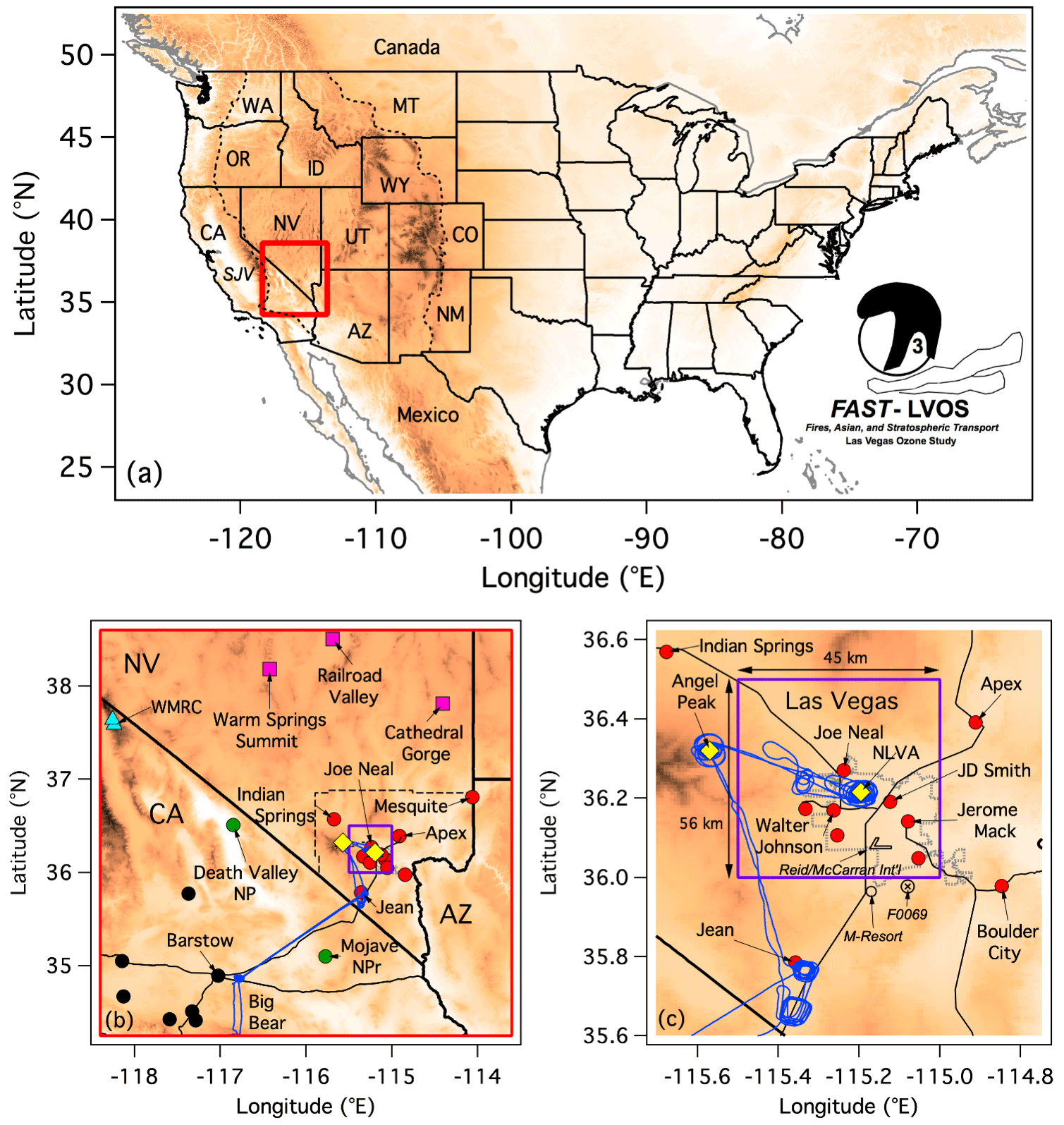
Figure 1 (a) Shaded relief map of the contiguous US showing the FAST-LVOS study domain (red box). The dashed black line outlines the US Intermountain West. The San Joaquin Valley (SJV) was studied the previous summer in the CABOTS field campaign. (b, c) Expanded views of the study area. The solid and dashed black lines in (b) mark the state and Clark County borders, respectively. The dotted black line in (c) outlines the Las Vegas metropolitan area. The color-filled circles mark regulatory O₃ monitors maintained by Clark County (red), the US National Park Service (green), and the California Air Resources Board (black). The magenta squares and cyan triangles show baseline monitors operated by the Nevada Department of Environmental Quality and White Mountain Research Center, respectively. The yellow diamonds show the locations of Angel Peak (AP) and the North Las Vegas Airport (NLVA; see text). The blue traces show the 28 June SA flight track, and the violet boxes outline the 0.25^∘ × 0.25^∘ (≈ 45 km H × 56 km W) FLEXPART receptor domain.

The air quality improvements in the US over the last 2 decades represent a major success, but the gains have not been uniform, with large decreases in the southeastern US (SEUS: Alabama, Florida, Georgia, North Carolina, South Carolina, and Virginia), where NO₂ and O₃ declined by 39 % and 25 %, respectively, but much smaller changes in the southwestern US (SWUS: Utah, Arizona, Colorado, and New Mexico), where a 38 % reduction in NO₂ led to an O₃ decline of just 11 %. The 4MDA8 O₃ decreased from 83 to 63 ppbv in the SEUS but only decreased from 77 to 69 ppbv in the SWUS. The weaker response to NO₂ reductions in the SWUS is attributed in part to increased oil and gas development (Pozzer et al., 2020) and in part to the much higher background O₃ in this region (EPA, 2013; Lefohn et al., 2014; Cooper et al., 2015). This background is derived from a variety of non-controllable ozone sources (NCOSs) including O₃ produced by photochemical reactions of anthropogenic emissions outside the US borders or by soils, vegetation, lightning, or wildfires and by naturally occurring O₃ transported downward from the stratosphere (Jaffe et al., 2018). The high mean elevations of Colorado (2078 m a.s.l.), Wyoming (2047 m a.s.l.), Utah (1864 m a.s.l.), Nevada (1681 m a.s.l.), and Idaho (1528 m a.s.l.), which make up the heart of the Intermountain West (IMW), i.e., the area of the US bounded by the Cascade (≤ 4392 m a.s.l.) and Sierra Nevada (≤ 4421 m a.s.l.) mountains to the west and the Front Range of the Rocky Mountains (≤ 4401 m a.s.l.) to the east (Fig. 1a), make this entire region particularly vulnerable to both stratospheric intrusions (Lin et al., 2012a) and pollution transported across the Pacific Ocean from East Asia (Lin et al., 2012b).

Background O₃ cannot be directly measured, but an upper limit can be estimated from measurements at remote “baseline” locations sufficiently removed from anthropogenic sources. Jaffe et al. (2018) estimated that the monthly mean MDA8 O₃ in the higher elevations of the IMW is around 50 ppbv in late spring, with the 4MDA8 O₃ concentrations exceeding 60 ppbv in some locations. These high baseline concentrations constitute more than 70 % of the 70 ppbv NAAQS set in 2015 (EPA, 2014) and limit the ability of western air quality managers to maintain surface O₃ concentrations below this standard through local control strategies (Cooper et al., 2015; Uhl and Moore, 2018; Faloona et al., 2020).

Concern about the potential impacts of stratospheric intrusions, Asian pollution, and other NCOSs on NAAQS attainment in the greater Las Vegas area motivated the first Las Vegas Ozone Study (LVOS) conducted by the NOAA Chemical Sciences Laboratory (CSL) in late May and June of 2013 (Langford et al., 2015b) in partnership with the Clark County (Nevada) Department of Air Quality (CCDAQ). The LVOS 2013 field campaign was organized around the truck-mounted TOPAZ (Tunable Optical Profiler for Aerosol and oZone) differential absorption lidar (Alvarez et al., 2011), which is part of the NASA-sponsored Tropospheric Ozone Lidar Network (TOLNet). The lidar was deployed for 6 weeks to a decommissioned US Air Force radar base on the summit of Angel Peak (AP: 36.32^∘ N, −115.57^∘ E; 2680 m above mean sea level, a.s.l.), about 45 km west of Las Vegas, in the Spring Mountains (Fig. 1c). The lidar measurements were augmented by in situ measurements of O₃ and CO and basic meteorological parameters.

The LVOS 2013 campaign documented several episodes in which the appearance of stratospheric intrusions, Asian pollution, or wildfire plumes at AP was followed by MDA8 O₃ concentrations greater than 70 ppbv at multiple regulatory monitors in Clark County and in some cases by exceedances of the 2008 O₃ NAAQS of 75 ppbv then in effect. Since stratospheric intrusions do not typically reach the relatively low elevations of Las Vegas (620 m a.s.l.), it was hypothesized that some of the high-O₃ episodes resulted from entrainment of mid-tropospheric O₃ layers (Langford et al., 2017) by the deep-convective boundary layers that form over the Mojave Desert (Seidel et al., 2012). This hypothesis could not be confirmed, however, because of the placement of the lidar above the valley floor, and a more extensive follow-up study, the Fires, Asian, and Stratospheric Transport–Las Vegas Ozone Study (FAST-LVOS), was conducted over the same time period in 2017 to (i) test the entrainment hypothesis, (ii) determine the representativeness of the LVOS 2013 results, and (iii) better characterize the different sources of surface O₃ in the Las Vegas Valley (LVV). In this paper, we present an overview of the FAST-LVOS campaign with brief examples highlighting the influence of stratospheric intrusions, Asian pollution, biomass burning, and both local and regional pollution on surface O₃ in Clark County and the greater IMW. The companion paper by Zhang et al. (2020) uses the GFDL-AM4 and GEOS-Chem global models to simulate these measurements and quantify the impacts of these processes on high-O₃ events in southern Nevada and the greater SWUS and IMW.

2 Background

Previous airborne and ground-based lidar measurements have shown that elevated O₃ layers are common features of the lower free troposphere between ≈ 3 and 6 km a.s.l. above California (Langford et al., 2012; Ryerson et al., 2013; Faloona et al., 2020) and southern Nevada (Langford et al., 2015b, 2017) in late spring and early summer, and it is well established that the US west coast is one of the global hotspots for deep stratosphere-to-troposphere transport (STT) of O₃ in springtime (Wernli and Bourqui, 2002; Sprenger and Wernli, 2003; James et al., 2003; Skerlak et al., 2014, 2015; Breeden et al., 2021). This occurs primarily through the formation of tropopause folds, tongues of lower stratospheric air that descend isentropically beneath the jet stream circulating around upper-level lows. These intrusions of dry, O₃-rich air often form near the end of the North Pacific storm track and descend behind the mixture of clean or polluted tropospheric air in the dry airstream (Wernli, 1997; Cooper et al., 2004; Trickl et al., 2014). They are thus an important mechanism for transport of East Asian pollution from the upper troposphere down to the boundary layer above the western US (Brown-Steiner and Hess, 2011; Lin et al., 2012a, b).

Tropopause folds typically follow one of two pathways as they reach the middle troposphere. Many intrusions, particularly those formed by deep closed lows, continue to curve cyclonically as they descend and wrap up above the surface low in the lower troposphere (Danielsen, 1964). These deep LC2 (lifecycle 2) intrusions (Thorncroft et al., 1993; Polvani and Esler, 2007) often reach the top of the boundary layer and sometimes even the surface at higher elevations (Schuepbach et al., 1999; Stohl et al., 2000; Bonasoni et al., 2000; Trickl et al., 2020). These intrusions were first described by Reed and Danielsen (1958) and have long been observed as steeply sloping tongues in ozone lidar curtains (Browell et al., 1987; Ancellet et al., 1994; Vaughan et al., 1994; Langford et al., 1996; Eisele et al., 1999).

Much less attention has been paid to the so-called LC1 (lifecycle 1) intrusions that are sheared anticyclonically from elongated troughs to form quasi-horizontal filaments in the middle and upper troposphere (Appenzeller and Davies, 1992; Appenzeller et al., 1996; Vaughan et al., 2001; Albers et al., 2021). These streamers are well-known features of satellite water vapor imagery (Manney and Stanford, 1987) and can stretch for thousands of kilometers. They usually roll up horizontally into a series of diminishing vortices to be irreversibly mixed into the free troposphere (Wirth et al., 1997; Vaughan and Worthington, 2000; Vaughan et al., 2001; Colette and Ancellet, 2006), but they can also be dissipated by moist convection (Langford and Reid, 1998). They are a significant source of background O₃ in the free troposphere (Albers et al., 2021) but usually remain well above the boundary layer and thus do not influence surface O₃ directly.

Both types of intrusions are most common in winter, when cyclonic activity is at a maximum, but stratospheric intrusions that form in late May and early June are more likely to affect compliance with the ozone NAAQS since (i) more O₃ is available for transport from the lower stratospheric reservoir in springtime (Albers et al., 2018), (ii) surface concentrations are higher because of increased photochemical production, and (iii) deeper afternoon mixed layers (Seidel et al., 2012) can potentially entrain some intrusions that would otherwise pass overhead. Stratospheric influence plays an important role in driving the observed year-to-year variability in springtime ozone air quality over the western US (Lin et al., 2015). The potential surface impacts of stratospheric intrusions and co-transported pollution decrease in summer after the jet stream migrates poleward into Canada, and deep convection lifts pollution higher into the upper troposphere over East Asia (Hudman et al., 2004; Brown-Steiner and Hess, 2011).

3 FAST-LVOS measurements and models

The FAST-LVOS field experiment was also organized around the TOPAZ lidar, which was upgraded with a new data acquisition system in 2015. This upgrade more than doubled the useful operating range of the lidar from ≈ 3 to 8 km, which allowed it to reach higher altitudes than was possible during LVOS 2013, even while operating from a much lower-elevation site at the North Las Vegas Airport (NLVA; 36.2^∘ N, −115.2^∘ E; 680 m a.s.l.), located about 8 km NW of downtown Las Vegas. NOAA CSL also brought a vertically staring Doppler lidar to the NLVA to characterize mixing between the boundary layer and free troposphere and a mobile laboratory with a more extensive suite of in situ measurements to the summit of AP. These primary measurements were supplemented by measurements from a single-engine Mooney TLS Bravo aircraft operated by Scientific Aviation, Inc. (SA) and by ozonesondes launched by the NOAA Global Monitoring Laboratory (GML) during four 2 to 4 d intensive operating periods (IOPs) initiated when the synoptic conditions showed that stratospheric intrusions or Asian pollution transport events were likely.

3.1 Primary measurements

3.1.1 NOAA CSL TOPAZ lidar

The TOPAZ truck arrived in Las Vegas on the morning of 17 May and was deployed to a secure CCDAQ enclosure on the north side of the NLVA. In addition to the lidar, the truck was equipped with an automated weather station (Airmar 150WX) and a commercial UV absorption O₃ monitor (2B Technologies model 205) that sampled air 5 m above the ground. The autonomous NOAA CSL vertically staring 1.5 µm micro-Doppler lidar was placed near the TOPAZ truck to measure aerosol backscatter and vertical wind variance for the estimation of boundary layer depths (Bonin et al., 2018). The two lidars were located near the CCDAQ wind profiler (Fig. 2, top) and visibility camera and about 500 m NNW of the National Weather Service (NWS) KVGT meteorological tower.

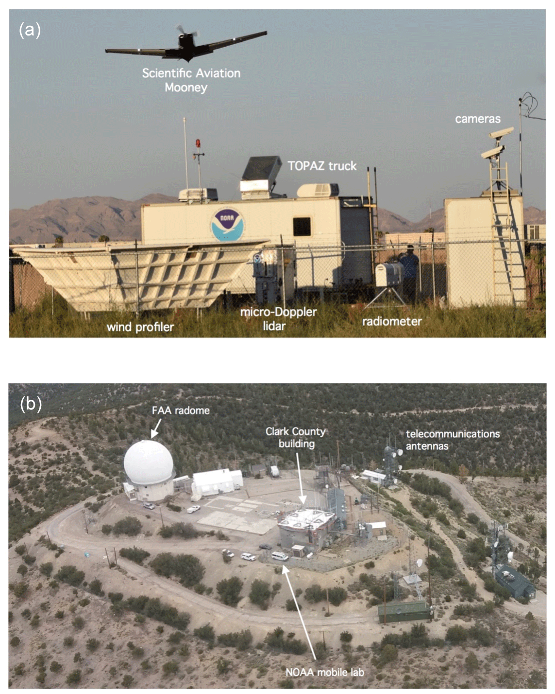
Figure 2 Photographs of the NLVA (a) and AP (b) FAST-LVOS ground sites. The NLVA photograph faces east and the AP photograph northwest. Note the TOPAZ scanning mirror housing near the center of the photograph with the lidar line of sight pointing away from the camera. The view of Angel Peak was taken from the SA Mooney aircraft and shows the NOAA mobile lab parked in the location occupied by the TOPAZ lidar during the 2013 LVOS campaign. Photographs by Andrew Langford (a) and Dani Caputi (b).​​​​​​​

TOPAZ uses a tuneable Ce:LiCaF solid-state laser and a unique transceiver configuration to profile O₃ and particulate backscatter (β) from just above the surface to ≈ 8 km above ground level (a.g.l.). The lidar points vertically but uses a large steerable mirror on top of the truck to sequentially deflect the co-axial laser beams and return signals along a series of elevation angles. The scanner line of sight was oriented to the east (parallel to the 7–25 runway) and successively tilted along paths 2, 6, 20, and 90^∘ above the horizon. This cycle was repeated every 8 min, and the vertical projections of the slant profiles merged with the zenith profile to create vertical ozone and backscatter profiles starting 27.5 ± 5 m above the ground, with the lowest measurements displaced about 800 m downrange. Ozone number densities were retrieved using two wavelengths (≈ 287 and 294 nm) with 30 m range gates and a smoothing filter that increased from 270 m wide at the minimum range (815 ± 15 m) to 1400 m wide at the maximum range. The ozone and backscatter profiles were computed simultaneously using an iterative procedure (Alvarez et al., 2011) incorporating the O₃ absorption cross-sections of Malicet et al. (1995) and temperature and pressure profiles interpolated from the 3 h National Centers for Environmental Prediction (NCEP) North American Regional Reanalysis (NARR) to account for the temperature dependence of the O₃ cross-sections and to convert the calculated O₃ number densities to mixing ratios. The effective O₃ vertical resolution increased from ≈ 10 m near the surface to 150 m at 500 m a.g.l. and 900 m at 6 km a.g.l. The maximum range was limited by solar background radiation during the day and decreased from about 8 to 6 km near midday. Backscatter from aerosols, smoke, and dust was also retrieved with 7.5 m resolution at 294 nm.

Total uncertainties in the 8 min O₃ retrievals are estimated to increase from ±3 ppbv below 4 km to ±10 ppbv at 8 km. The upgraded TOPAZ system was extensively compared with measurements from the same SA Mooney aircraft used here as well as the NASA Alpha Jet (Hamill et al., 2016) in the 2016 CABOTS field campaign (Langford et al., 2019) and with electrochemical concentration cell (ECC) ozonesondes and ground-based TOLNet lidars in the 2016 Southern California Ozone Observation Project (SCOOP) (Leblanc et al., 2018). Both intercomparisons showed excellent agreement within the stated uncertainties in the measurement techniques, particularly when the spatial and temporal differences introduced by the different sampling methods are considered.

3.1.2 NOAA CSL Mobile Laboratory

The van-based CSL mobile laboratory (Wild et al., 2017) was equipped with instruments to measure O₃, CO, water vapor (H₂O), carbon dioxide (CO₂), CH₄, NO, NO₂, total reactive nitrogen oxides (NO_y), nitrous oxide (N₂O), and meteorological parameters. The NO, NO₂, NO_y, and O₃ measurements were made with a custom-built cavity ring-down spectrometer (CRDS) (Washenfelder et al., 2011; Wild et al., 2014; Womack et al., 2017); a commercial (Picarro) wavelength-scanned CRDS to measure CO₂ and CH₄ (Peischl et al., 2013); and a modified commercial (Los Gatos) instrument using off-axis-integrated cavity output spectroscopy (OA-ICOS) to measure N₂O, CO, and H₂O (Coggon et al., 2016). Additional details about these instruments can be found in the references. Ozone was also measured by a commercial (2B Tech, Model 205) ultraviolet photometer, and these data were used to fill in the gaps during brief periods when the CRDS instrument was offline. There were no aerosol measurements.

The mobile laboratory carried the same automated weather station (Airmar 150WX) as the TOPAZ truck and was also equipped with differential GPS and sonic anemometers to measure absolute wind speed and direction while the van was moving. The laboratory was parked on the southeastern edge of the AP summit overlooking Kyle Canyon, the primary corridor for upslope transport from the LVV, for most of the campaign. This is the same location (Fig. 2, bottom) occupied by the TOPAZ truck during LVOS 2013 and provides an unobstructed fetch to the west, south, and east. Northerly winds (≈ 335 and 65^∘) were perturbed by one of the nearby buildings, but winds from this direction were uncommon during the study. A few drives were conducted between AP and the LVV on 23–25 May during IOP1 and again on 15 and 17 June. These measurements will be described elsewhere. The van was also relocated to the NLVA for an intercomparison with the instruments on the SA Mooney on 15 June. All of the measurements described here are from AP.

The first LVOS campaign in 2013 used the relationships between the O₃, H₂O, and CO measured on AP to infer the history of the air masses sampled on the summit (Langford et al., 2015b). This was made possible because of the relative remoteness and high elevation of the site, which minimized the influences of nearby NO_x or CO emissions and surface deposition, and by the lack of rainfall and extreme aridity of the Mojave Desert, which makes water vapor a semi-conserved tracer. Since CO has a tropospheric lifetime of ≈ 60 d and originates primarily from soil emissions and combustion processes (Holloway et al., 2000), concentrations are lower in the stratosphere than in the free troposphere and terrestrial boundary layer. Conversely, O₃ concentrations are much higher in the stratosphere than in the troposphere. Thus, O₃ and CO tend to be negatively correlated in mixtures of stratospheric and free-tropospheric air, which is also very dry, but positively correlated in mixtures of free-tropospheric air and urban pollution or biomass burning plumes. The marine boundary layer is far removed from most natural and anthropogenic sources of CO and O₃ and has low concentrations of both (Clark et al., 2015). Thus, the relationships between these three parameters can be used to separate the influences of stratospheric intrusions and Asian pollution from regional pollution and wildfires and distinguish air that descended from the lower stratosphere or upper troposphere from air advected inland from the Pacific Ocean.

This empirical approach was much improved by the addition of N₂O, NO, NO₂, NO_y, CH₄, and CO₂ measurements in the 2017 FAST-LVOS campaign. Nitrous oxide has a much longer tropospheric lifetime than CO (> 100 years) and originates primarily from natural and fertilized soils (Tian et al., 2019) and the oceans (Tian et al., 2020). It is thus well mixed throughout the free troposphere, with much lower concentrations in the stratosphere, and can be used as a tracer for recent agricultural and oceanic influences and stratospheric intrusions (Hintsa et al., 1998; Assonov et al., 2013). The CH₄ measurements provide another useful tracer for Asian pollution (Xiao et al., 2004) as well as oil and gas (Peischl et al., 2018), agricultural (Peischl et al., 2012), and biomass burning (Delmas, 1994) influences. The NO, NO₂, and NO_y measurements can be used to identify air masses influenced by biomass burning or by local, regional, and Asian pollution. In particular, the short lifetime (≈ 2–4 h) of NO_x (Laughner and Cohen, 2019) makes these measurements a useful tracer for pollution from the LVV. The CO₂ measurements can also help identify pollution and biomass burning influences, although interpretation of these measurements is complicated by the strong diurnal variations created by photosynthetic uptake.

3.1.3 Meteorological measurements

The temperature, pressure, relative humidity, wind speed, and wind direction from the automated weather stations in the TOPAZ truck at the NLVA and the mobile laboratory on AP are summarized in Fig. S1 in the Supplement. The NLVA measurements were supplemented by the NWS measurements from the KVGT tower, and vertical wind information was also obtained from the radar wind profiler, ozonesondes, and aircraft. The automated micro-Doppler lidar measurements near the TOPAZ truck were used to calculate hourly averaged boundary layer heights (Bonin et al., 2018), which ranged from ≈ 2 to 4 km in the afternoon. Mixed layer heights were also derived from the potential temperature and relative humidity profiles acquired by the GML ozonesondes (8 km distant) and from the afternoon (00:00 UT or 17:00 Pacific Daylight Time, PDT) radiosondes launched from the Harry Reid (formerly McCarran) International Airport (NWS station identifier KVEF) about 15 km to the south. The figure also shows solar radiation measurements from a site in Henderson near KVEF (cf. Fig. 1f) that were obtained from the University of Utah MesoWest network (https://mesowest.utah.edu, last access: 16 August 2021) and from the Spring Mountain Youth Camp (SMYC), which occupies the former cantonment area of the decommissioned Air Force base and lies ≈ 800 m west and 120 m below the AP summit. The SMYC measurements were obtained from the Western Regional Climate Center (WRCC) (http://www.wrcc.dri.edu/weather/smyc.html, last access: 16 August 2021).

3.2 Supplemental measurements

The supplemental ozonesonde and aircraft sampling during the intensive operating periods (IOPs) provided important context for the lidar and surface measurements. The four IOPs were conducted on 23–25 May, 31 May–2 June, 10–14 June, and 27–30 June (no ozonesondes were launched on 14 and 27 June). The NOAA Global Monitoring Laboratory (GML) launched a total of 30 ozonesondes (1 to 4 ozonesondes per day) from a park adjacent to the CCDAQ Joe Neal monitoring site located about 8 km northwest of the NLVA during the four IOPs. The ozonesondes (Sterling et al., 2018) measured O₃ concentrations to altitudes well above the 8 km range of the lidar and recorded temperature, relative humidity, and wind profiles, which helped characterize the synoptic context.

The SA Mooney conducted daily flights between the NLVA and Big Bear, CA (cf. Fig. 1b), during the four FAST-LVOS IOPs, logging a total of 90 flight hours over 15 d. The aircraft carried a pilot and flight scientist, along with a 2B Technologies Model 205 O₃ monitor, an Aerodyne Research cavity attenuated phase shift (CAPS) NO₂ monitor, and a Picarro 2301f wavelength-scanned cavity ring-down spectrometer (WS-CRDS) to measure CO₂, CH₄, ethane (C₂H₆), and H₂O (Trousdell et al., 2016). The 2B O₃ data were sampled at 2 s intervals, which corresponds to a mean distance of 150 m at the typical level flight speed of 75 m s⁻¹. The standard TLS flight plan (Fig. 1b and c) began with a vertical profile to about 5 km a.s.l. above North Las Vegas after take-off. The aircraft then flew to AP and spiralled down around the summit to ≈ 3 km a.s.l. (cf. Fig. 2, bottom). From there, the aircraft headed to Jean, NV (924 m a.s.l.), where the southernmost CCDAQ O₃ monitor is located, and conducted another profile. The pilot then followed the I-5 corridor before diverting south to Big Bear, CA, where the aircraft landed and refueled. The return leg began with a profile above Barstow, CA, before following the I-5 corridor back to Clark County with additional profiles above Jean, AP, and North Las Vegas if fuel permitted. The default flight plan was modified as necessary to account for air traffic control requirements.

3.3 Ancillary measurements

The CCDAQ maintains a network of continuous air monitoring stations (CAMSs) for O₃ and other parameters (e.g., NO₂, fine (PM_2.5) and coarse (PM₁₀) particulates, meteorology) in the LVV and surrounding areas (cf. Fig. 1). The CCDAQ also operates an upper-air station consisting of a radar wind profiler and profiling radiometer at the NLVA (cf. Fig. 2, top) and automated visibility cameras at the NLVA and M-Resort (cf. Fig. 1). The CAMS network included 11 active O₃ monitors during the FAST-LVOS campaign, with the Joe Neal (C75), Walter Johnson (C71), and JD Smith (C2002, since deactivated) monitors located within 8 km of the NLVA (cf. Fig. 1c). The hourly averaged measurements from the TOPAZ monitor at the NLVA agreed with the Joe Neal and Walter Johnson measurements to within 3 % on average, with linear regression coefficients of determination of R² = 0.87 (NLVA-C75), R² = 0.76 (NLVA-C71), and R² = 0.75 (C75-C71) when the Doppler lidar showed the boundary layer was well mixed. The Joe Neal and Walter Johnson O₃ measurements are discussed in Sects. 8 and 9 along with those from the more distant Apex (C22, 32 km), Jean (C1019, 49 km), Indian Springs (C7772, 58 km), and Mesquite (C23, 121 km) monitors located outside the LVV. The CCDAQ also operated a temporary O₃ monitor at the SMYC; these measurements averaged ≈ 8 % lower (R² = 0.91) than both the CRDS and 2B measurements from the mobile laboratory on the summit and are not used in our analyses.

Surface O₃ measurements from other monitors operated by federal, state, local, and tribal agencies outside of Clark County were obtained from the EPA Air Quality System (AQS) (https://www.epa.gov/aqs, last access: 16 August 2021) and Clean Air Status and Trends Network (CASTNET) (https://www.epa.gov/castnet, last access: 16 August 2021). The Nevada Division of Environmental Protection (NVDEP) also operated three portable solar-powered monitors at the Warm Springs Summit (WSSU; 38.184^∘ N, −116.425^∘ E; 2307 m a.s.l.), Railroad Valley (RRVA; 38.504^∘ N, −115.694^∘ E; 1413 m a.s.l.), and Cathedral Gorge State Park (CGSP; 37.810^∘ N, −114.410^∘ E; 1513 m a.s.l.) to measure baseline O₃ during FAST-LVOS. Measurements were previously made at these three sites as part of the Nevada Rural Ozone Initiative (NVROI) (Fine et al., 2015a, b; Gustin et al., 2015). Measurements from two remote research monitors operated by the White Mountain Research Center (WMRC) (Burley and Bytnerowicz, 2011) were also shared with the FAST-LVOS project. The WMRC maintains the highest continuously operating surface O₃ monitors in the continental US at White Mountain Summit (WMS; 37.634^∘ N, −118.256^∘ E; 4342 m. a.s.l.) and Barcroft Observatory (BCO; 37.590^∘ N, −118.239^∘ E; 3879 m a.s.l.) located ≈ 280 km NW of AP (cf. Fig. 1b).

3.4 Model support

Planning for the FAST-LVOS day-to-day activities and IOPs relied primarily on long-range weather forecasts from the NCEP Global Forecast System (GFS) obtained from the University of Wyoming (http://weather.uwyo.edu/models/fcst/gfs003.shtml, last access: 16 August 2021) and 4 d 1^∘ × 1^∘ O₃ and CO forecasts from the NOAA/NESDIS RAQMS (http://raqms-ops.ssec.wisc.edu/, last access: 16 August 2021) (Pierce et al., 2003) model. The RAQMS model also provided boundary conditions for the 13 km resolution NOAA rapid refresh RAP-Chem (https://rapidrefresh.noaa.gov/RAPchem, last access: 15 August 2021) model. The daily forecasts from these two models were supplemented by GOES-West water vapor imagery and other satellite products obtained from the NOAA/NESDIS Regional and Mesoscale Meteorology Branch (RMBB; http://rammb.cira.colostate.edu, last access: 16 August 2021) at the Colorado State University. Data interpretation was aided by the NASA Modern-Era Retrospective-analysis for Research and Applications (MERRA-2) reanalysis (https://fluid.nccs.nasa.gov/reanalysis/classic_merra2/, last access: 16 August 2021) online plotting resources (Gelaro et al., 2017); NOAA Air Resources Laboratory (ARL) HYSPLIT trajectories (Stein et al., 2015); and stratospheric, Asian pollution, and biomass burning tracers calculated with 0.25^∘ horizontal resolution using the FLEXPART particle dispersion model driven by the European Centre for Medium-Range Weather Forecasts (ECMWF) operational (0.5^∘ × 0.5^∘) model (Brioude et al., 2007, 2009). The RAQMS, RAP-Chem, and FLEXPART models used in the study are described in more detail in the FAST-LVOS final report (https://csl.noaa.gov/projects/fastlvos/FAST-LVOSfinalreport604318-16.pdf, last access: 7 December 2021). The FAST-LVOS measurements were also simulated by the GEOS-Chem (≈ 50 × 50 km² horizontal, 0.2 to 1.0 km vertical resolution in the free troposphere) and AM4 (≈ 0.25^∘ × 0.3125^∘ horizontal, 0.1 to 1.0 km vertical resolution in the free troposphere) chemistry–climate models; these efforts are described in the companion paper by Zhang et al. (2020).

4 Meteorological contexts

The FAST-LVOS campaign can be divided into two meteorologically distinct periods, a late spring period from mid-May to mid-June and an early summer period from mid-June through the end of June. The Synoptic Discussion for May 2017 from the National Centers for Environmental Information (NCEI) (https://www.ncdc.noaa.gov/sotc/synoptic/201705, last access: 16 August 2021) describes the jet stream as being very active in the late spring period, with a series of closed lows and upper-level troughs crossing the contiguous US every few days. These cyclonic systems spawned a series of stratospheric intrusions that appear as potential vorticity (PV) enhancements (Duncan et al., 2021) in the 300 hPa (≈ 9.5 km a.s.l.) NASA MERRA-2 Reanalysis plots in Fig. 3a–d. GOES water vapor images coinciding with the PV analyses are displayed in Fig. S2. The first extratropical cyclone, designated L₁ in Fig. 3a, passed through Nevada before the official start of the campaign on 20 May, but the next three low-pressure systems, labeled L₂, L₃, and L₄ in Fig. 3b–d, were targeted by IOPs on 23–25 May, 31 May–2 June, and 11–14 June. The solar radiation data in Fig. S1 show the appearance of cirrus ahead of the cold fronts as well as perturbations in the normal diurnal variations in pressure, temperature, dew point, and winds created by thermally driven regional (e.g., plains–mountain) and mesoscale (e.g., valley and slope) circulations (Stewart et al., 2002). There was no measurable precipitation, but the temperatures on AP dropped below freezing on the nights of 17–18 May and 11–12 June, and the cold fronts decreased the depth of the afternoon boundary layers above the NLVA to ≈ 2 km, or roughly the elevation of AP above the valley.

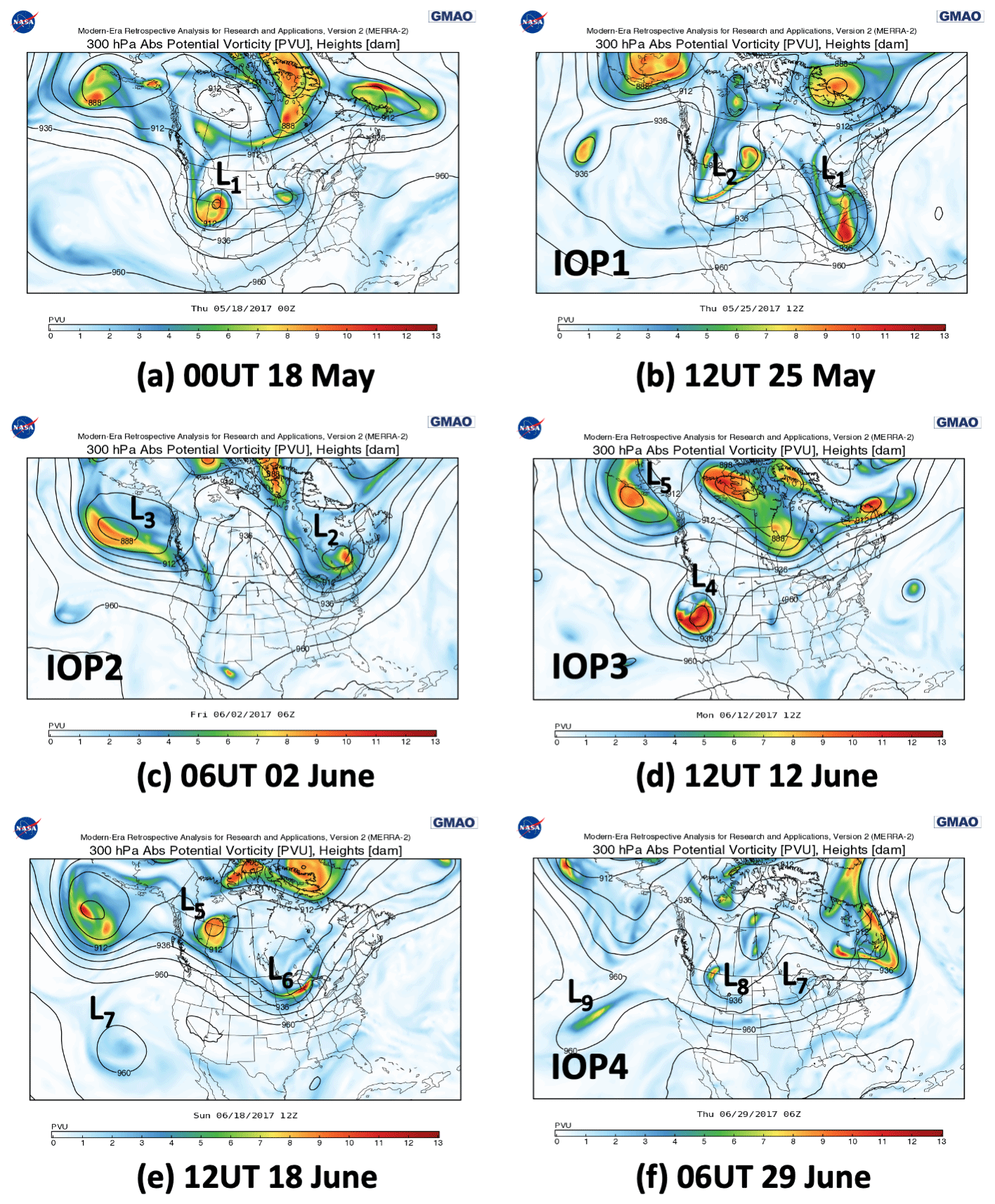
Figure 3 MERRA-2 300 hPa Absolute potential vorticity and geopotential heights (dam) at (a) 00:00 UT 18 May, (b) 12:00 UT 25 May, (c) 06:00 UT 2 June, (d) 12:00 UT 12 June, (e) 12:00 UT 18 June, and (f) 06:00 UT 29 June.

The jet stream retreated north into Canada in the wake of L₄, and the NCEI Synoptic Discussion for June 2017 confirms that the expanding subtropical ridge seen in Fig. 3e dominated the weather across the SWUS for the rest of the campaign (https://www.ncdc.noaa.gov/sotc/synoptic/201706, last access: 16 August 2021). The ridge brought clear skies, dry conditions, and record high temperatures to Clark County, and June 2017 was the third-hottest in Las Vegas since official record keeping began in 1948, and the extreme temperatures and dry conditions exacerbated multiple wildfires across the SWUS. The high temperatures at the NLVA exceeded 41 ^∘C (106 ^∘F) each day during the last 2 weeks of the study, and the daily records for Las Vegas were tied or exceeded on 5 straight days from 20 to 24 June. The official high of 47.2 ^∘C (117 ^∘F) at Harry Reid International Airport on 20 June, the last day of astronomical spring, tied the all-time Las Vegas record. Coincidentally, this record was also tied on the final day of the first LVOS campaign (30 June 2013). The daily high temperatures abated slightly to 42–43 ^∘C during the last few days of the campaign and IOP4, when a weak cold front associated with the shallow trough (L₈) in Fig. 3f passed through the LVV. The temperatures on AP were typically 10–15 ^∘C lower due to its higher elevation.

5 Overview of results

5.1 TOPAZ profiles

TOPAZ operated for an average of ≈ 12 h a day over 45 consecutive days (17 May–30 June) during FAST-LVOS, accumulating a total of 4026 profiles or 537 h of observations. Approximately 60 % of the profiles were acquired between the hours of 09:00 and 17:00 PDT, but there were several extended runs including a 60 h continuous session from 11–13 June. The O₃ and β profiles are summarized as time–height curtain plots in Figs. 4 and 5, respectively. The scalloped appearance of the individual curtains is caused by the diurnal variation in background solar radiation, which determines the measurement signal-to-noise and thus the maximum achievable altitude. The dark-gray curves show the boundary layer heights from the Doppler lidar, and the red boxes outline the four IOPs. The colored stripe along the bottom of Fig. 4 shows the NLVA measurements from the in situ monitor in the truck. Preliminary TOPAZ measurements from the afternoon of 17 May caught the remnants of a deep cyclonic intrusion from the closed low (L₁) in Fig. 3a, and free-tropospheric layers and filaments were present in nearly all of the profiles measured between mid-May and mid-June. The low backscatter in Fig. 5 shows that these layers were not created by biomass burning, and most of the layers were higher (> 4 km a.g.l) and more persistent than would be expected for pollution lofted from the Los Angeles Basin by the “mountain chimney effect” (Langford et al., 2010), but this process may have contributed to some of the lower-lying “residual layers” in the ozone curtains (e.g., 16 June). This suggests that most of the higher-O₃ layers were stratospheric intrusions or Asian pollution plumes, a conclusion supported by the AM4 and GEOS-Chem simulations (Zhang et al., 2020). Free-tropospheric O₃ layers appeared less frequently after the jet stream retreated into Canada, and photochemical production increased rapidly as the subtropical ridge moved into the SWUS. The highest O₃ concentrations were usually measured in the boundary layer after mid-June, although Fig. 4 shows that this pattern was briefly interrupted on 18–19 June, when the anticyclonic circulation transported clean marine air deep into the IMW. High O₃ was present both in and above the boundary layer during the last 3 d of the campaign, when IOP4 was conducted.

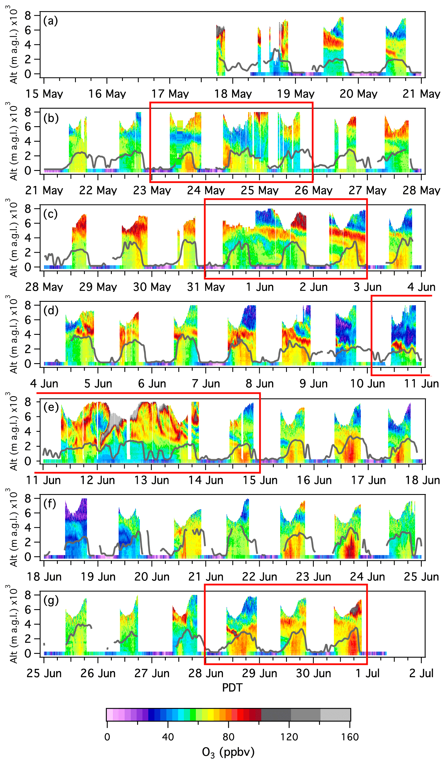
Figure 4 Time–height curtain plots showing the TOPAZ ozone measurements from the NLVA. The axes are altitude (Alt) above ground level and Pacific Daylight Time (PDT). The continuous ribbon along the bottom shows the measurements from the in situ surface monitor in the TOPAZ truck, and the dark-gray curves show the boundary layer heights inferred from the co-located Doppler lidar measurements. The red boxes bracket the four IOPs.

Figure 5 Same as Fig. 4, but for the TOPAZ backscatter measurements.

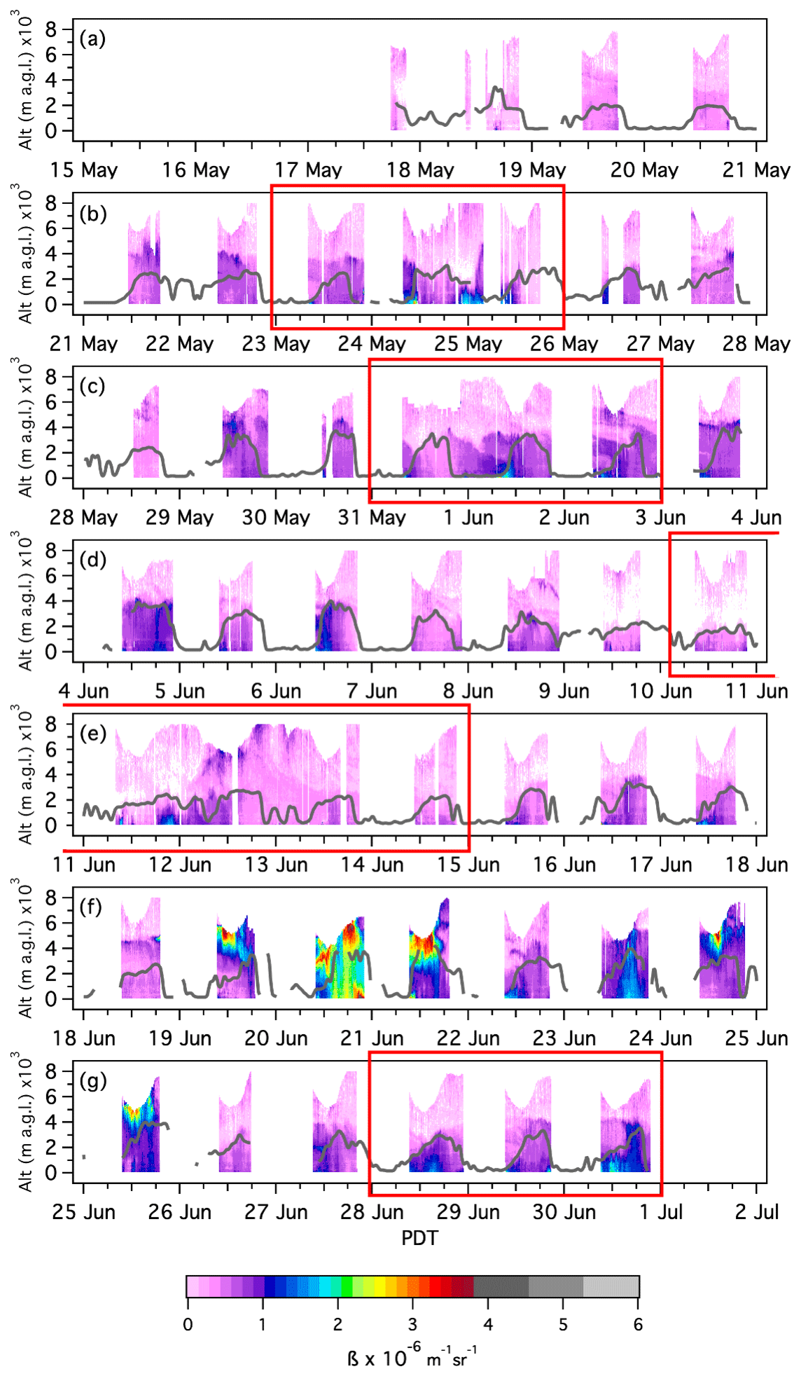
The backscatter curtains in Fig. 5 show that TOPAZ measured relatively low backscatter during most of the campaign. The aerosol loading was usually highest in the boundary layer, but comparisons to the near-IR Doppler lidar measurements and ozonesondes show that the gradients in the UV profiles were usually too weak to reliably define the boundary layer height. The backscatter above the top of the boundary layer increased abruptly on 19 June, when smoke from fires in Arizona and Mexico drifted into the LVV, and high backscatter was measured both in and above the boundary layer on 20 June, when smoke from the much closer Holcomb Fire reached Las Vegas. Note that the boundary layer height determination relied heavily on the vertical velocity variance profile when dispersed smoke was present. These measurements will be described in more detail elsewhere along with those from 23–26 June, when smoke from other regional wildfires reached Las Vegas and possibly contributed to the high surface O₃ measured on those days.

5.2 Mobile laboratory measurements

The nearly continuous 1 min averaged in situ O₃ measurements from the AP mobile laboratory are summarized in the top panel of Fig. 6; the lower panels plot the corresponding CO, CO₂, CH₄, N₂O, NO, NO₂, and NO_y measurements. As noted above, the lack of rainfall and extreme aridity of the Mojave Desert allow us to use water vapor as a semi-conserved tracer, and each of the time series is colorized by the co-measured H₂O to show whether the sampled air came from the lower stratosphere or upper troposphere (dry: violet–blue) or from the terrestrial (moderate: green–yellow) or marine (moist: yellow–red) lower troposphere. The letters A–G identify specific transport episodes that are examined in more detail below. The mobile laboratory measured 1 min O₃ mixing ratios in excess of 80 ppbv on 8 of the 43 measurement days in the campaign and mixing ratios in excess of 70 ppbv on 17 d. The MDA8 O₃ averaged 60 ± 8 ppbv and exceeded the NAAQS on 4 d. Some of the highest O₃ concentrations were measured in very dry air with low NO₂ and NO_y during the night and early morning (e.g., 8–9 June, episode C, and 11–12 June, episode D), but high O₃ was also measured in more humid air with elevated NO₂ and NO_y on some afternoons (e.g., 2 June, episode B). The AP wind measurements show that all of the short-lived nocturnal peaks coincided with strong southwesterly winds, while the broader afternoon peaks were associated with weaker southeasterly upslope flow. The lowest O₃ concentrations of the campaign were measured on 18–19 June in very moist air transported inland by the anticyclonic flow around the subtropical ridge seen centered over southern Nevada in Fig. 3e.

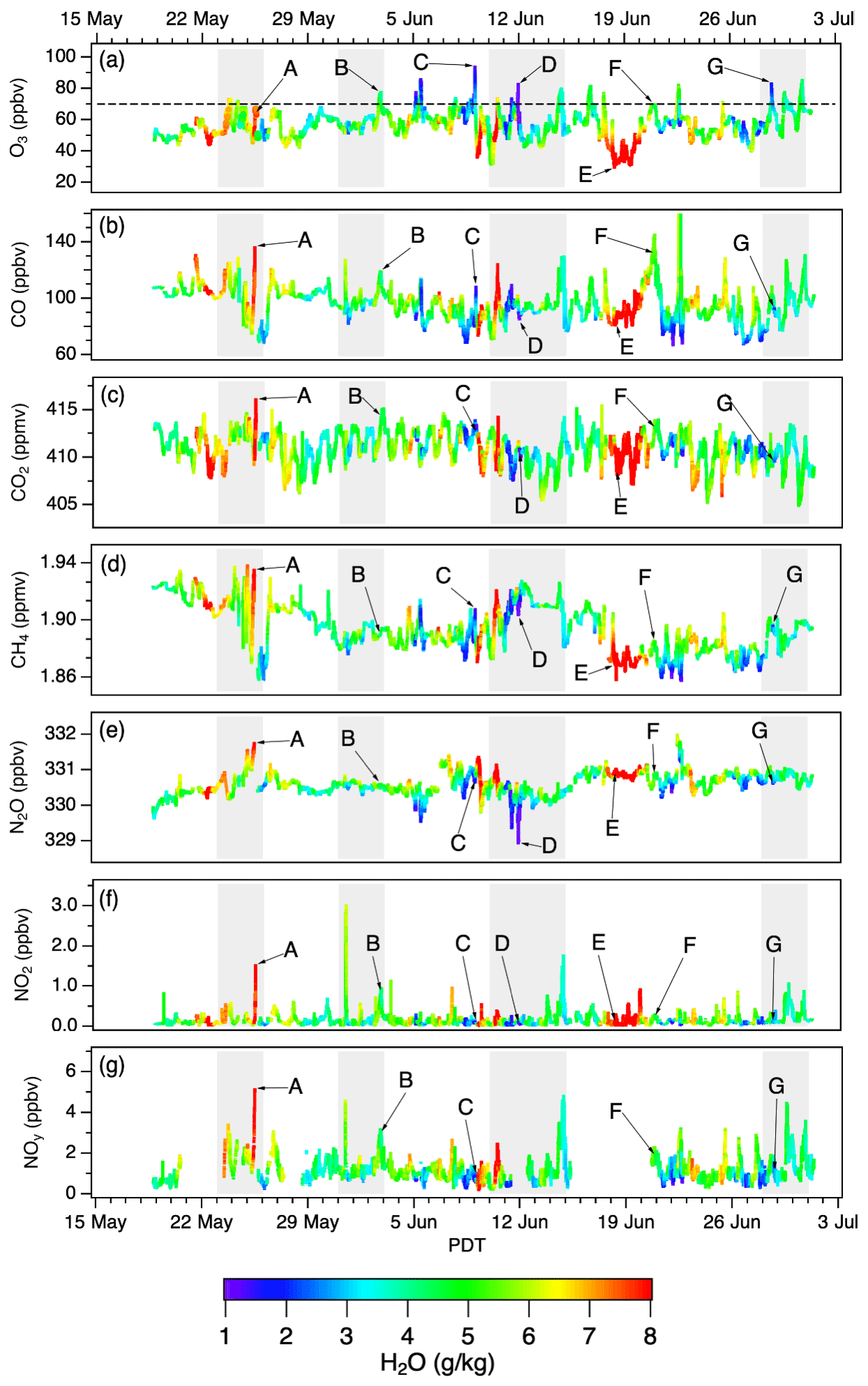
Figure 6 Time series of the AP 1 min in situ measurements color-coded by the co-measured H₂O. The dashed black line in (a) shows the 2015 NAAQS of 70 ppbv. The gray regions bracket the four IOPs. The measurements labeled A–G are discussed in the text.

5.3 Comparisons and validation

The vertical scanning capability of the TOPAZ lidar allows direct comparisons with nearby surface in situ monitors. Figure 7a compares time series of the O₃ mixing ratios retrieved at 27.5 ± 5 m a.g.l. (red) with the in situ measurements sampled 5 m a.g.l. at the truck (gray). The two series are in excellent agreement (±1 %, R² = 0.91) when the co-located Doppler lidar showed the boundary layer to be > 2500 m deep (black). The TOPAZ lidar was not normally run overnight, but Fig. 7a shows that the only significant differences between the time series occurred during a 24 h run through the night of 31 May–1 June (IOP2) when O₃ near the truck was titrated by NO emitted from nearby combustion sources. These emissions did not affect the TOPAZ concentrations retrieved about 20 m high and 800 m down range. The nocturnal losses were much smaller on 25 May and 7–12 June, when winds from the passing cold fronts dispersed the NO_x emissions and disrupted the shallow nocturnal inversion layers. Figure 7b is similar to Fig. 7a but compares the NLVA in situ measurements with the TOPAZ mixing ratios at 2000 m a.g.l., the elevation of AP. Although TOPAZ frequently measured higher O₃ aloft on 7–12 June when the boundary layer was relatively shallow (Fig. S1), these measurements are also in good agreement (±1 %, R² = 0.76) when the boundary layer was deeper than 2500 m.

Figure 7 Time series comparing the TOPAZ O₃ mixing ratios with the NLVA and AP in situ measurements. (a) TPZ (0.03 km) and NLVA surface monitor in the TOPAZ truck, (b) TPZ 2.0 km a.g.l. and NLVA surface monitor, (c) NLVA and AP surface monitors, and (d) TPZ 2.0 km a.g.l. and AP surface monitor. The gray bands show the four IOPs. The dashed horizontal lines show the 2015 NAAQS of 70 ppbv. The red points highlight measurements made when the mixed layer was more than 2500 m deep.

Figure 7c compares the in situ measurements from the NLVA (gray) with those from AP (red). The most obvious difference between the time series is the lack of surface deposition and NO_x titration on AP, which was exposed to free-tropospheric air during the night. The black points show that mixing ratios were similar (±4 %, R² = 0.46) when the boundary layer above the NLVA was > 2500 m. One notable exception is the measurements from 23 June, when the measurements in the LVV may have been influenced by smoke from the Brian Head Fire in southwestern Utah (cf. Fig. 5f). Although difficult to see in Fig. 7c, the AP O₃ concentrations typically lagged those at the NLVA on days with well-developed upslope flow, including the 4 AP exceedance days (14, 16, 29, and 30 June). A key assumption of the FAST-LVOS experimental design was that the air sampled on the summit of AP was representative of the air entrained by the mixed layer above the LVV. The similarity between the 2000 m a.g.l. TOPAZ retrievals and the mobile laboratory O₃ measurements in Fig. 7d shows that this was generally the case when the boundary layer was > 2500 m deep. The time series are in good agreement (±4 %, R² = 0.60) under these conditions if the measurements from 23 June are excluded.

6 Intensive operating periods

The aircraft and ozonesonde profiles acquired during the four IOPs provided spatial context for the lidar measurements and helped distinguish stratospheric intrusions from Asian pollution. The planning and successful execution of these intensives relied on the ability of the RAQMS (96 h) and RAP-Chem (48 h) models to predict stratospheric intrusion and pollution transport events more than 48 h in advance so that the aircraft and ozonesonde teams could return to Las Vegas from their home stations. Examples of the model forecasts are shown in Fig. 8, which displays the O₃ and CO forecasts for 12:00 UT 12 June (cf. Fig. 3d). The left panels of Fig. 8 show the 96 h total O₃ (top) and CO (bottom) at 320 K (≈ 500 hPa or 5.8 km a.s.l. above Las Vegas) from RAQMS initialized at 12:00 UT on 7 June, and the right panels show the 36 h RAP-Chem O₃ and CO 500 hPa forecasts initialized at 00:00 UT on 11 June. Note that the higher-resolution RAP-Chem model gets its boundary conditions from the RAQMS model. This example shows that the RAQMS model captured both the timing and location of the stratospheric intrusion–Asian pollution event 4 d out or 3 d before the start of IOP3 on 10 June. The retrospective MERRA-2 PV analyses in Fig. 3 and FLEXPART stratospheric ozone (STTO3) and Asian CO (ASIACO) tracer distributions (https://csl.noaa.gov/projects/fastlvos/FAST-LVOSfinalreport604318-16.pdf, last access: 7 December 2021) in Figs. 9 and 10, respectively, show that stratospheric air and/or Asian pollution was present in the middle and upper troposphere above Nevada during each of the IOPs. The correspondence between the 96 h RAQMS forecasts in Fig. 8 and the retrospective FLEXPART distributions in the third columns of Figs. 9 and 10 is particularly impressive.

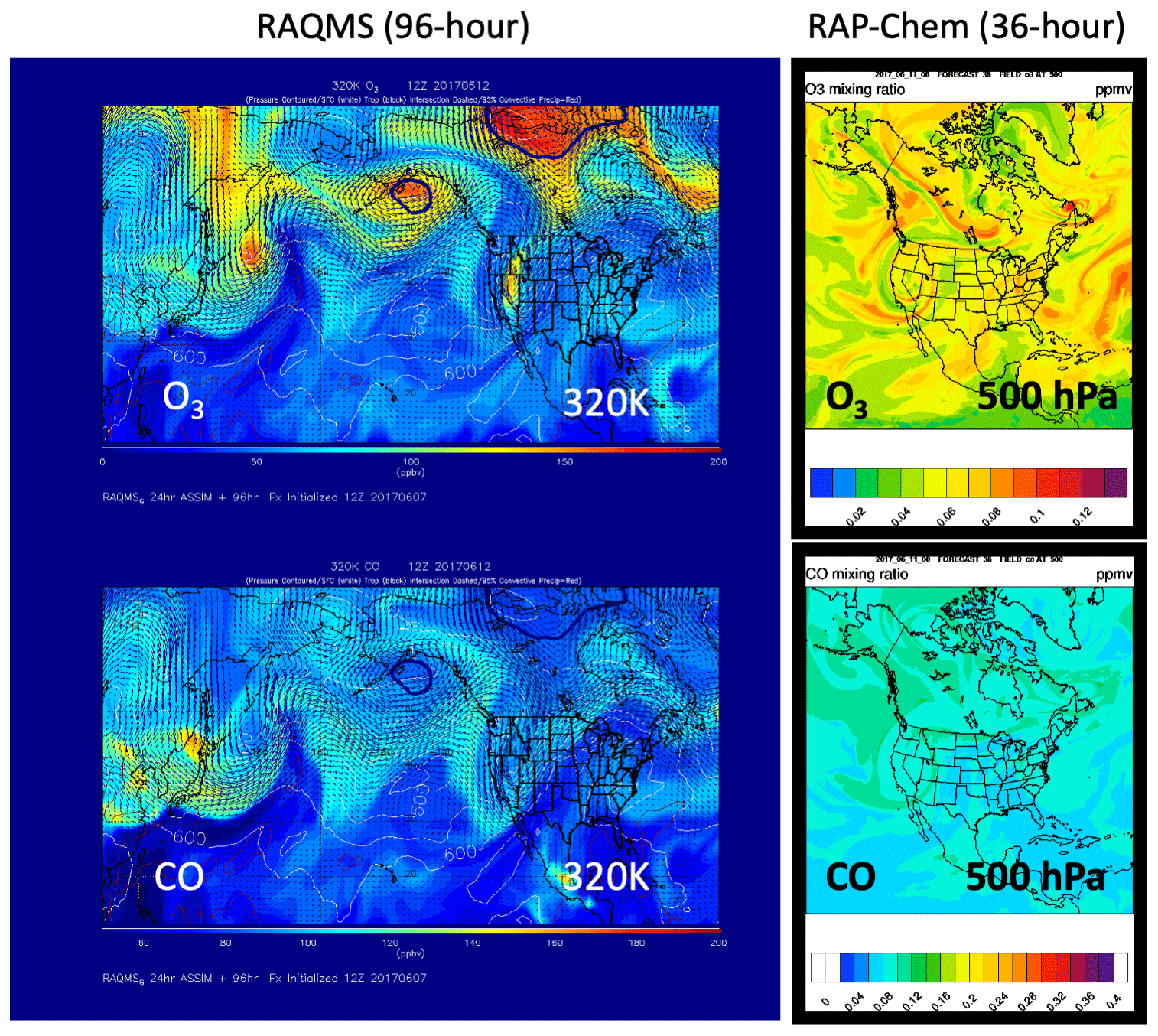
Figure 8 RAQMS (left) and RAP-Chem (right) O₃ (top) and CO (bottom) forecasts for 12:00 UT 12 June 2017. The 320 K RAQMS forecasts were initialized at 12:00 UT 7 June, the 500 hPa RAP-Chem forecasts at 00:00 UT 11 June.

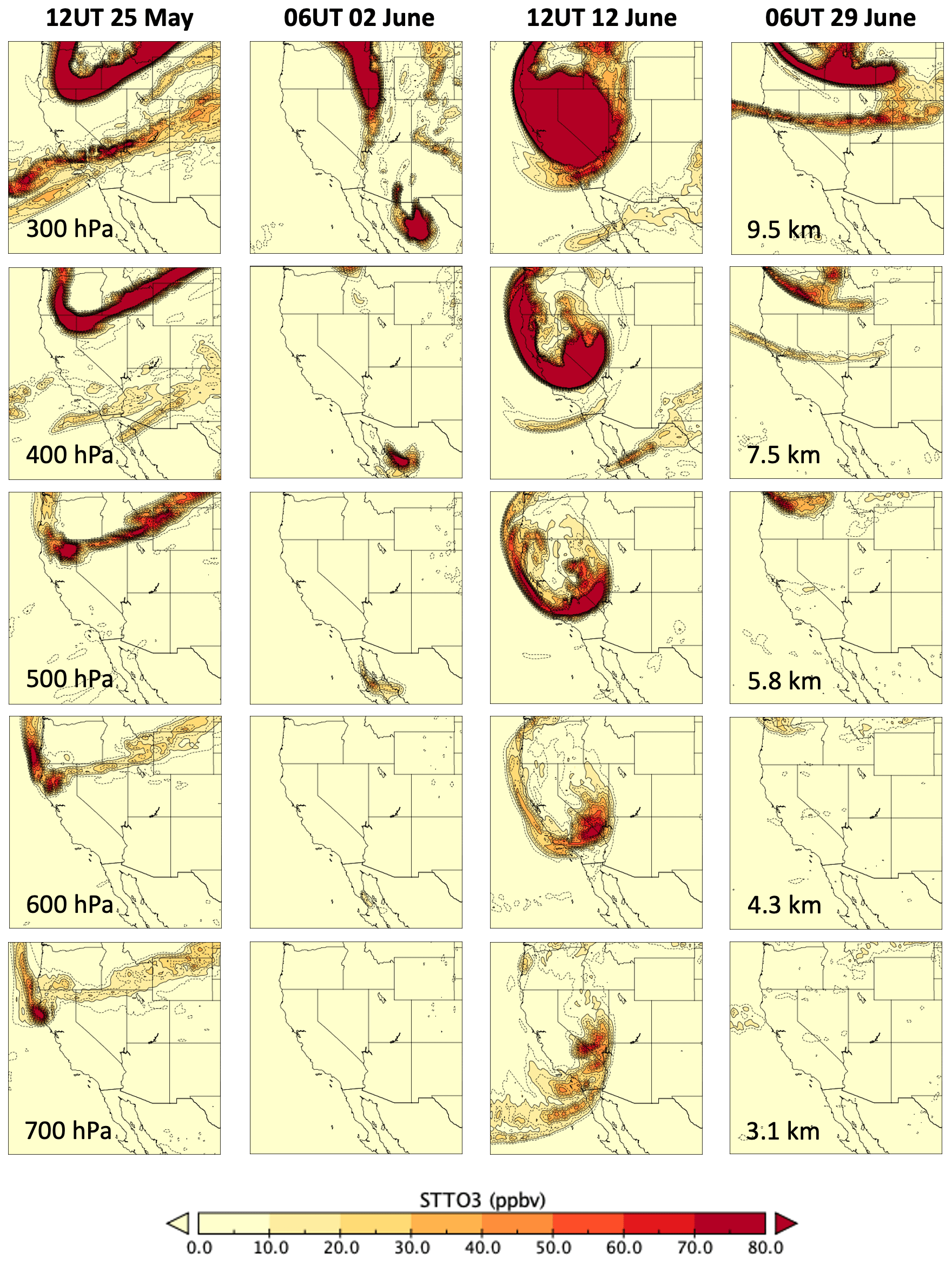
Figure 9 FLEXPART STTO3 tracer distributions during the four IOPs. The plots show the distributions, from left to right, at 12:00 UT 25 May, 00:00 UT 2 June, 12:00 UT 12 June, and 06:00 UT 29 June and from top to bottom at 300, 400, 500, 600, and 700 hPa. The approximate altitudes above sea level near Las Vegas corresponding to the different pressure surfaces are shown in the panels on the far right. The heavy black contour lines (e.g., in the upper left panel) indicate that the scale is saturated.

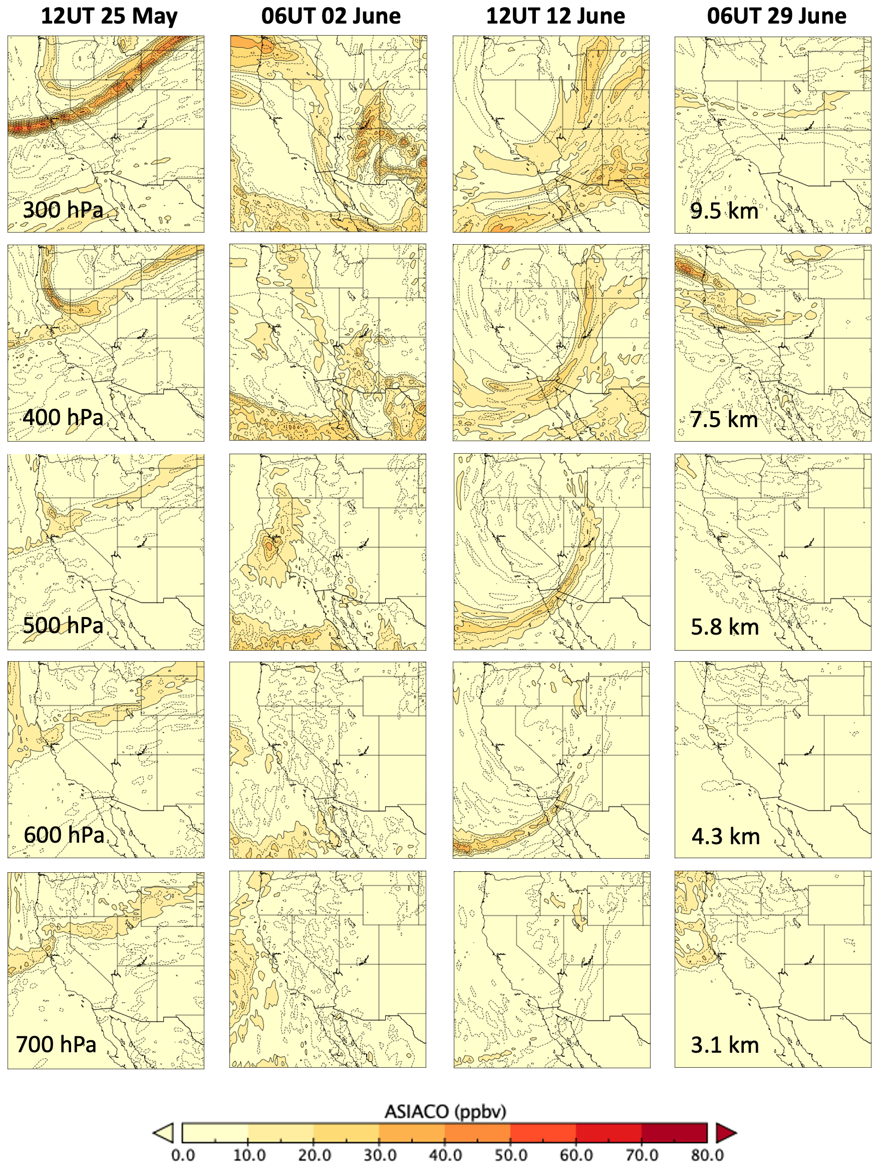
Figure 10 Same as Fig. 9, but for the ASIACO tracer.

The curtain plots in Fig. 4 show that the TOPAZ lidar measured high O₃ in the middle and upper troposphere during each of the IOPs; the expanded 3 d curtain plots in Figs. 11–14 show these measurements in more detail. The superimposed horizontal ribbons represent the NLVA and AP surface measurements and the nearly vertical ribbons the ascending profiles from the ozonesondes. Those portions of the descending profiles within 20 km of the NLVA are also plotted. The NLVA and AP surface wind measurements and continuous Doppler lidar boundary layer heights are also overlaid on the curtains, with the boundary layer heights derived from the ozonesonde potential temperature profiles (open black circles) plotted for comparison. The heavy arrows at the top of each plot correspond to the MERRA-2 analyses in Fig. 3. The labels A, B, D, and G match the corresponding peaks in Fig. 6.

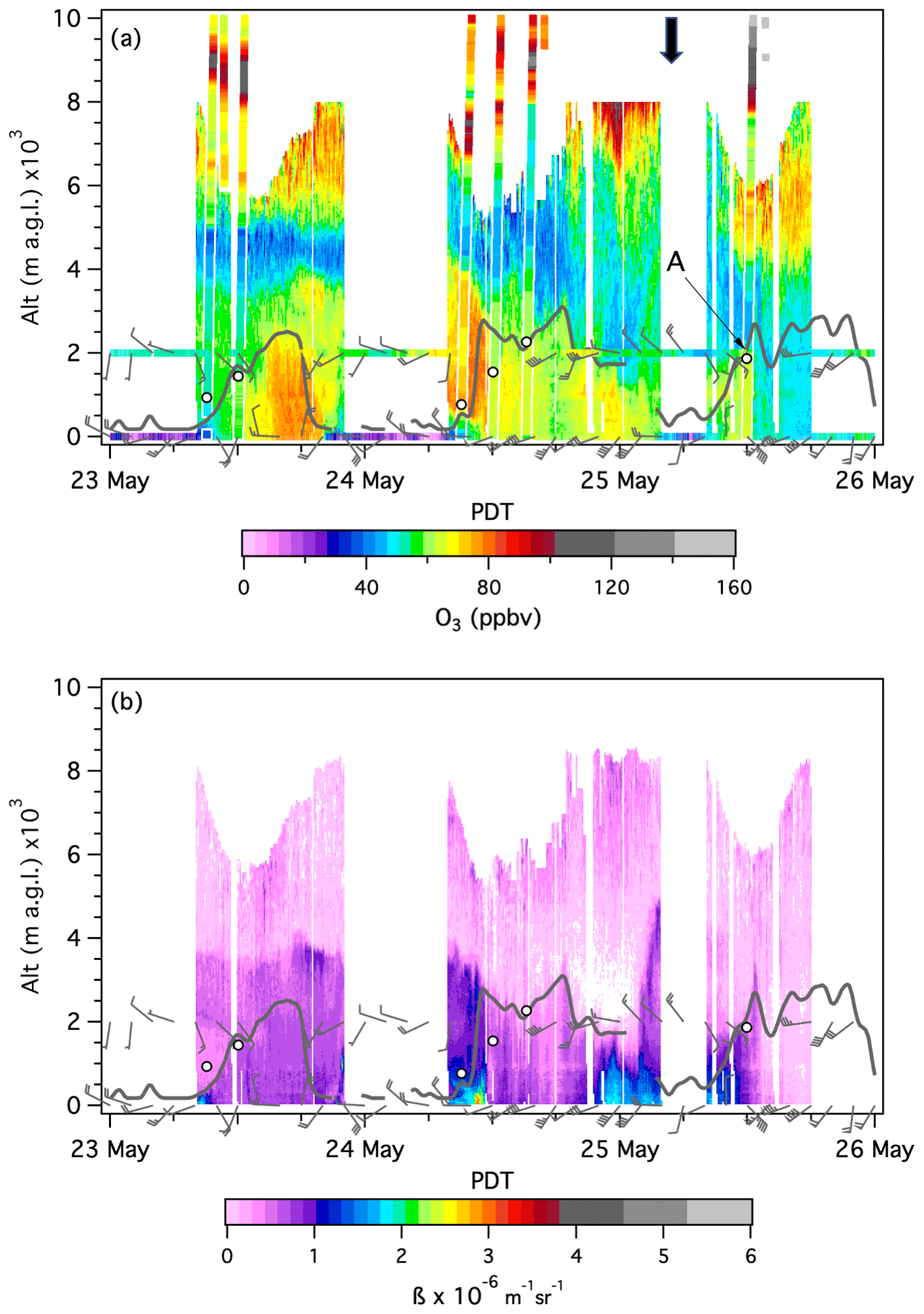
Figure 11 Time–height curtain plots similar to those in Figs. 4 and 5, but expanded to better show the TOPAZ (a) ozone and (b) backscatter measurements during IOP1. The dark-gray curves represent the boundary layer heights derived from the co-located Doppler lidar measurements. The superimposed horizontal bands in (a) show the AP and NLVA in situ O₃ measurements, and the near-vertical colored bands show the Joe Neal ozonesonde profiles. The barbs in both panels show the AP and NLVA surface winds and the open circles the mixing heights inferred from the ozonesondes. The heavy black arrow above (a) corresponds to the 12:00 UT 25 May PV plot from Fig. 3b. The 300 hPa surface lies at approximately 9 km a.g.l. The label “A” is the same as in Fig. 6.

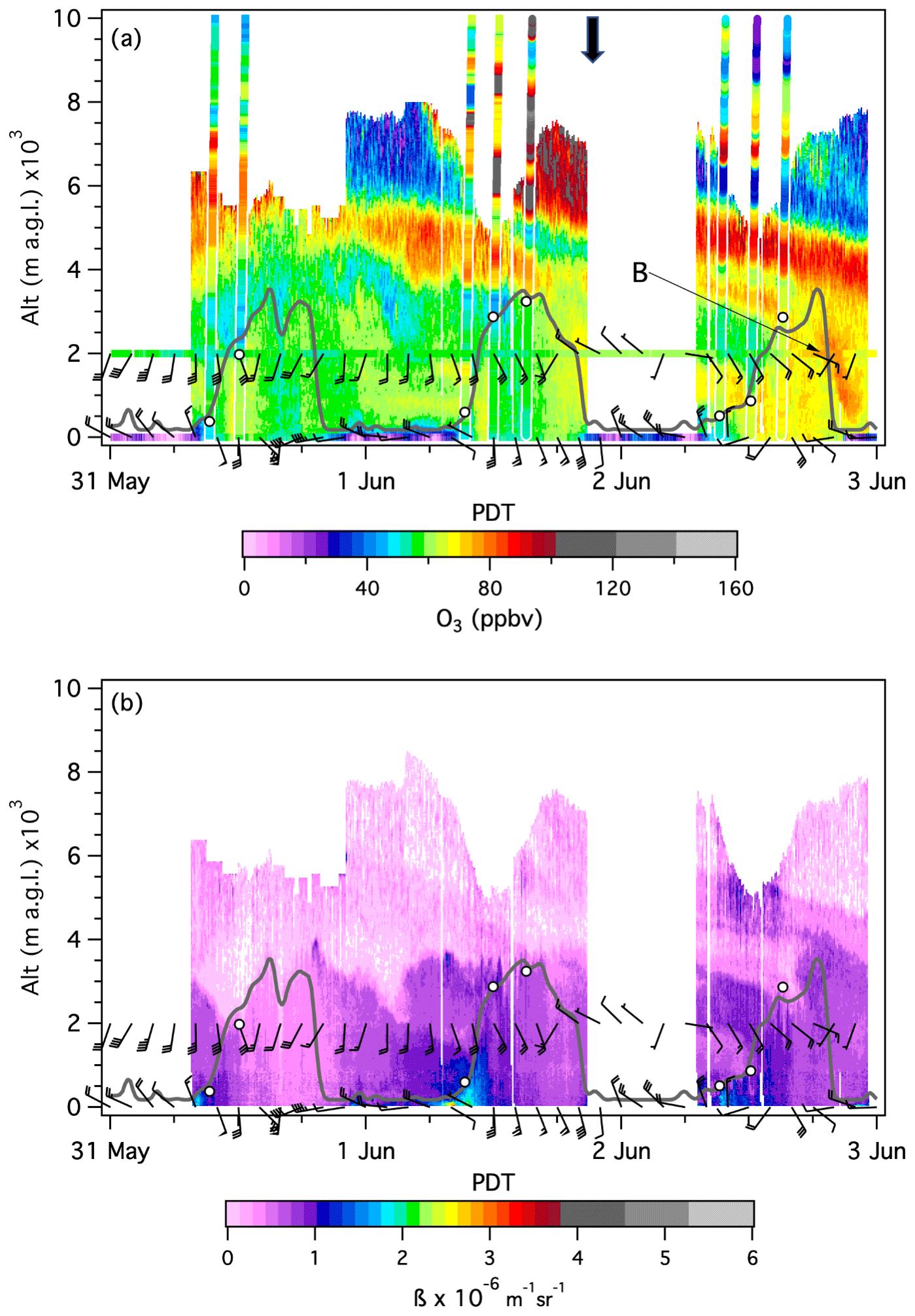
Figure 12 Same as Fig. 11, but for IOP2. The heavy black arrow corresponds to the 06:00 UT 2 June 300 hPa plot in Fig. 3c.

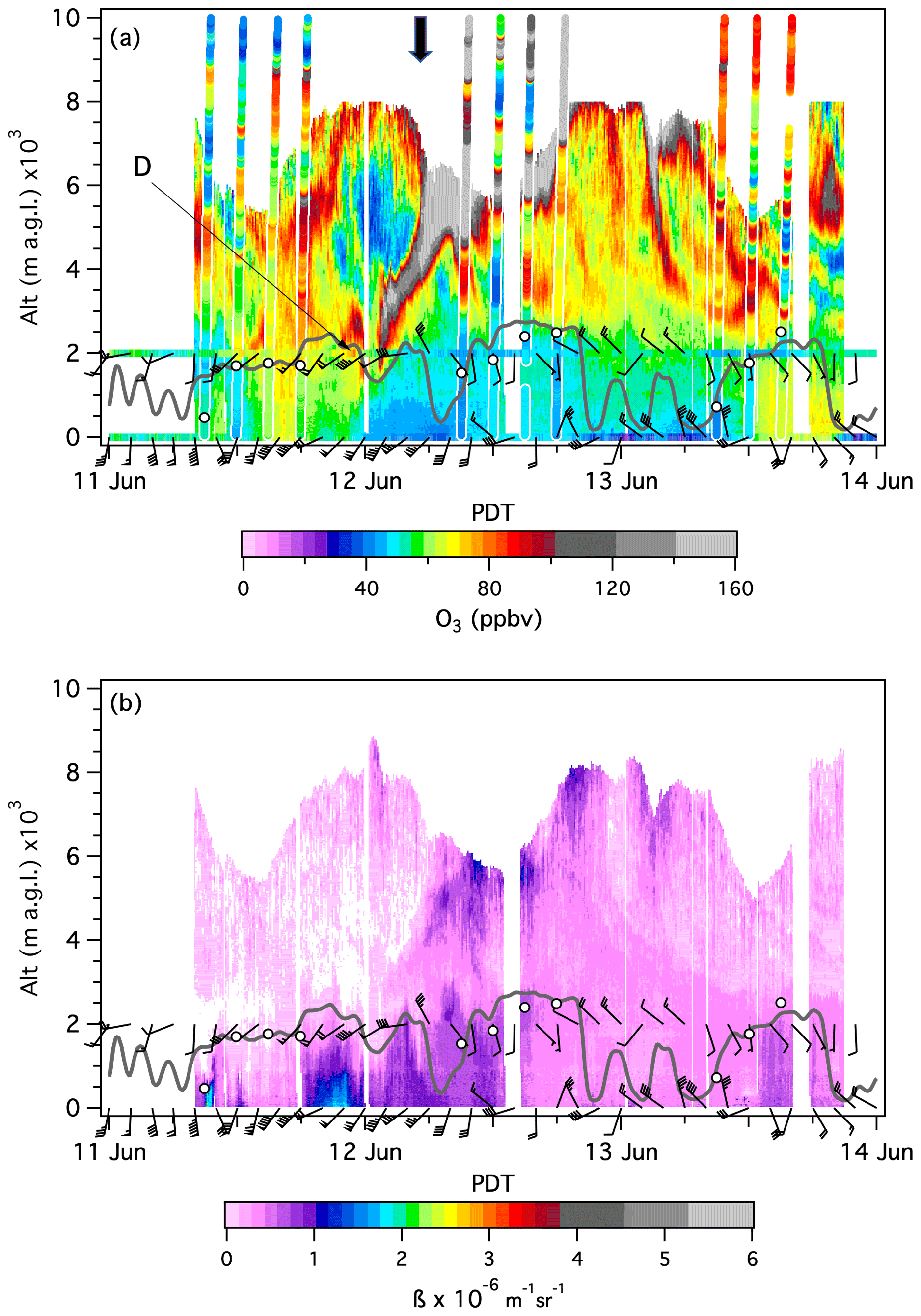
Figure 13 Same as Fig. 11, but for IOP3. The heavy black arrow corresponds to the 12:00 UT 12 June 300 hPa plot in Fig. 3d.

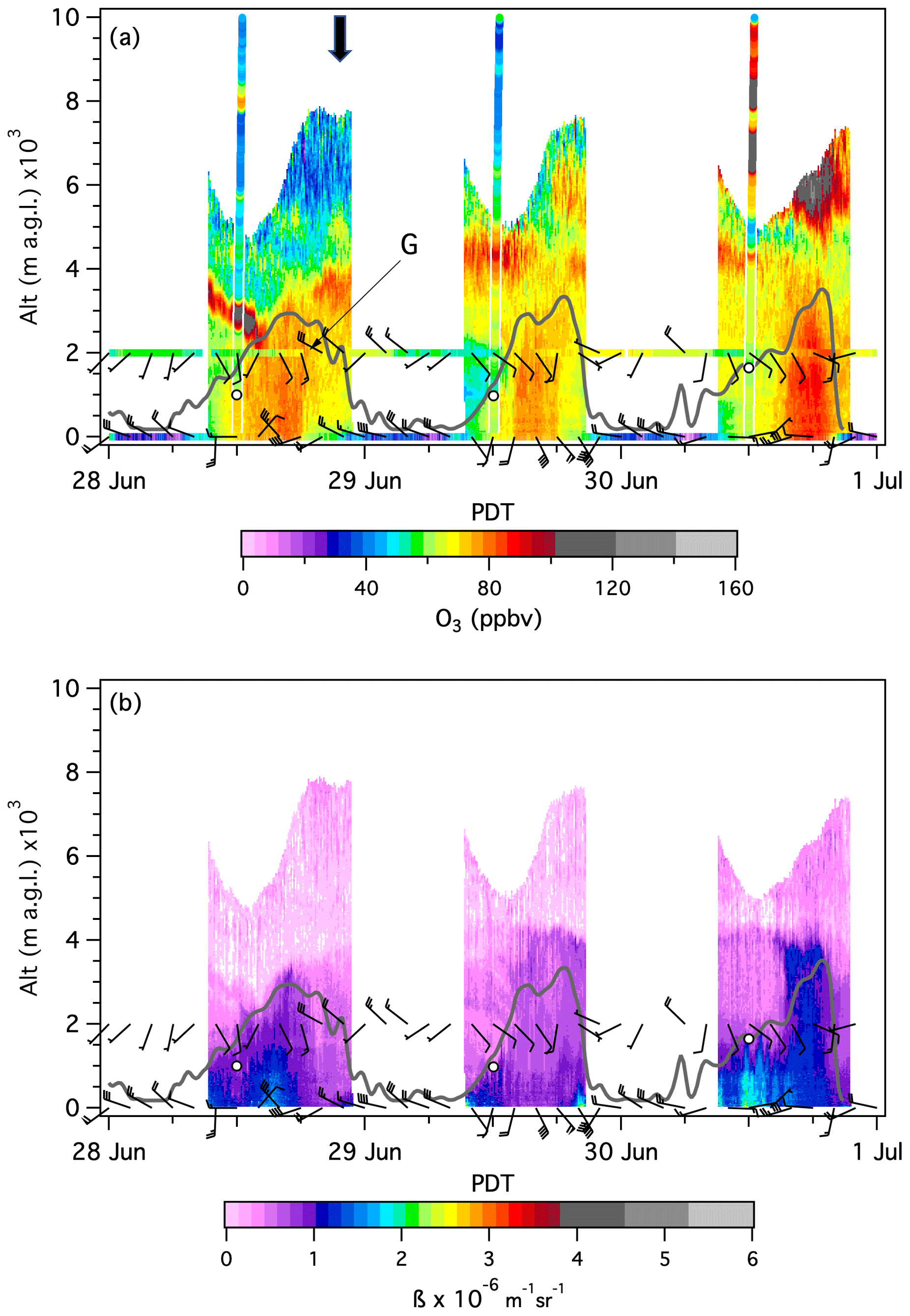
Figure 14 Same as Fig. 11, but for IOP4. The heavy black arrow corresponds to the 00:00 UT 29 June 300 hPa plot in Fig. 3f.

The SA aircraft profiles overlap with the midday ozonesonde profiles and are omitted from the curtain plots for clarity, but Fig. 15 shows longitudinal transects of the sections of the outbound (left) and inbound (right) flight legs between the NLVA and AP on 25 May (IOP1), 2 June (IOP2), 12 June (IOP3), and 28 June (IOP4). The flight tracks are colorized by the O₃ measurements, and the plots also show the mean lidar and ozonesonde profiles and surface O₃ measurements from the roughly 1 h interval bracketing the NLVA and AP profiles. Ozonesondes were only launched between 09:00 and 15:00 PDT and thus did not overlap with the return flight legs. These plots underscore the good agreement between the different FAST-LVOS O₃ measurements and support the assumption that the air above AP was usually representative of the air above the LVV. Similar plots colorized by H₂O and CH₄ are displayed in Figs. S2 and S3. Figure 16 shows the measured O₃ mixing ratios along the outbound flight legs from the NLVA to Big Bear and the inbound flight legs back to Jean. The AP profiles and TOPAZ measurements are omitted from these plots as are the afternoon profiles above the LVV. In the following sections, we briefly describe each of the IOPs and compare the upper-air measurements with the FLEXPART STTO3 and ASIACO tracer distributions. More complete descriptions of these measurements are planned for future publications.

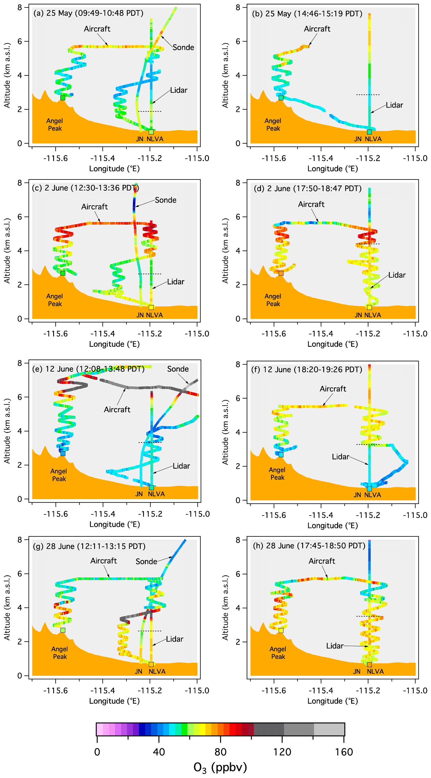
Figure 15 Ozone mixing ratios measured by the lidar, ozonesonde, and aircraft and by the AP, Joe Neal (JN), and NLVA surface monitors during the outgoing (left) and returning (right) flights on (a, b) 25 May, (c, d) 2 June, (e, f) 12 June, and (g, h) 28 June. The dashed horizontal lines show the boundary layer height inferred from the NLVA Doppler lidar measurements.

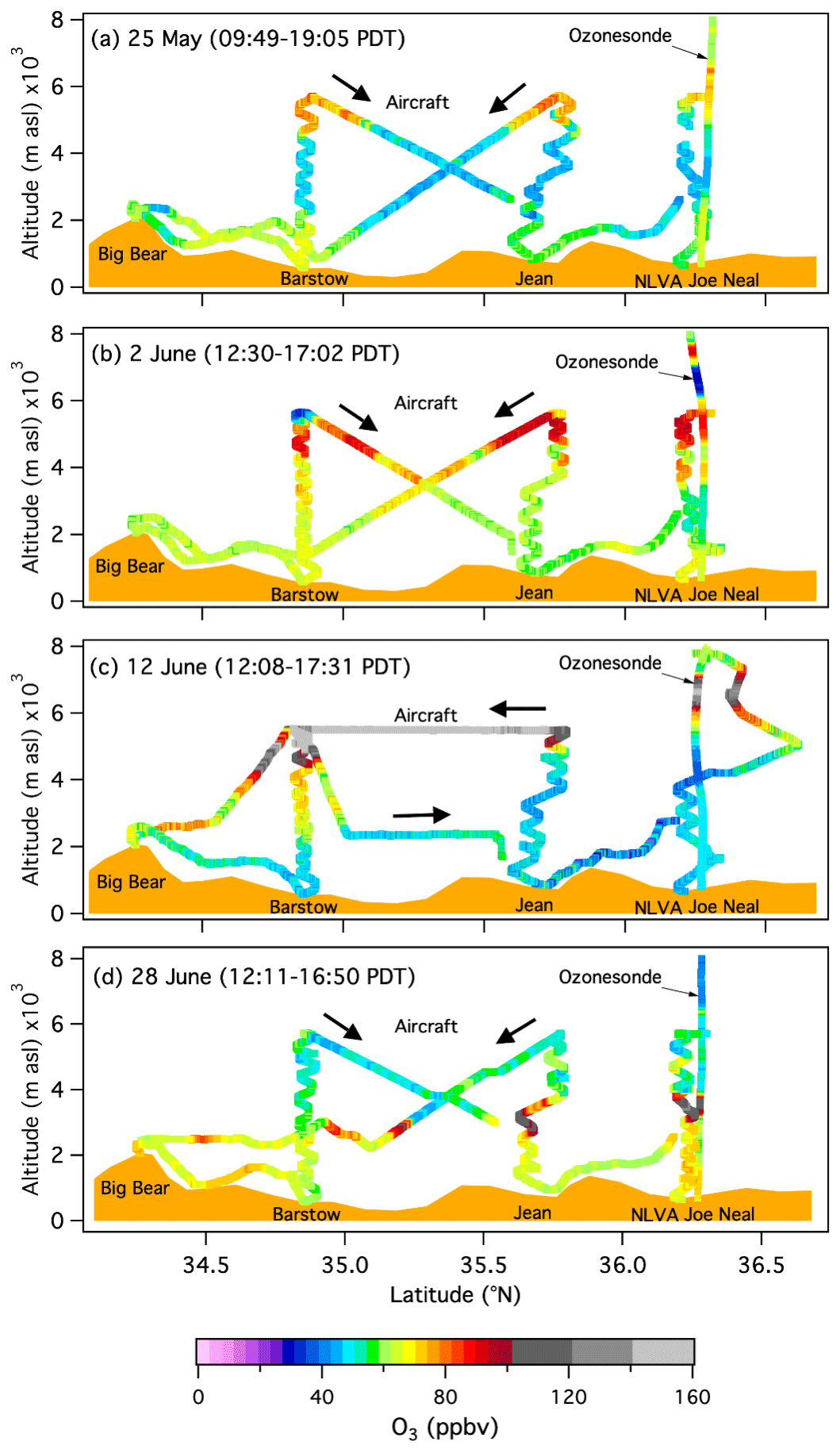
Figure 16 Ozone mixing ratios measured by the ozonesonde and aircraft on the flights to and from Big Bear on (a) 25 May, (b) 2 June, (c) 12 June, and (d) 28 June. The TOPAZ measurements and AP aircraft profiles are omitted for clarity, as are the Jean and NLVA aircraft profiles from the return legs. The terrain profile is approximate.

6.1 IOP1: 23–25 May

The first IOP was timed to coincide with the arrival of the trough (L₂) poised above the northern IMW in Fig. 3b. The PV analysis for the morning (12:00 UT) of 25 May shows a deep cyclonic intrusion wrapping around L₂, and the FLEXPART STTO3 plots in the first column of Fig. 9 show a deep cyclonic intrusion descending almost vertically to 700 hPa above northern Nevada and California. The PV analysis in Fig. 3b also shows a thin anticyclonic streamer stretching across southern Nevada from the tip of L₁, now an elongated trough over the eastern US, and FLEXPART shows this shallower feature on the 300 and 400 hPa surfaces. The ASIACO tracer distributions in the first column of Fig. 10 show Asian pollution mingled with the cyclonic intrusion and in a deep narrow band stretching across northern Nevada between the cyclonic and anticyclonic intrusions. Analysis of satellite CO measurements and the GFDL-AM4 and GEOS-Chem model simulations by Zhang et al. (2020) also found a large Asian pollution component in these layers.

The curtain plots for 23–25 May in Fig. 11 show layers with more than 100 ppbv of O₃ above the LVV on all 3 d, but the layers were above the ≈ 6 km a.s.l. altitude ceiling of the SA Mooney on the first 2 d. The aircraft was able to reach the more diffuse band with 75 to 80 ppbv of O₃ seen above 4.5 km a.g.l. on 25 May, however, and the plots in Figs. 15 and 16 show that this layer extended to the south at least as far as Barstow (cf. Fig. 1).

Figure S3 shows that the air in this layer was extremely dry, but the absence of a corresponding CH₄ enhancement in Fig. S4 suggests that this layer was primarily of stratospheric origin. The lidar, aircraft, and ozonesonde measurements also show that the high O₃ aloft was separated from the boundary layer by a layer of continental air with much lower O₃ concentrations, and there was no obvious local mixing of the O₃ aloft into the boundary layer. The GFDL-AM4 simulations also found little evidence for stratospheric or Asian pollution influences in Clark County surface air but estimated Asian contributions of 8–15 ppbv of O₃ to the surface along the areas of northern California, Idaho, and Wyoming lying beneath the bands seen in the 700 hPa STTO3 and ASIACO FLEXPART analyses.

The GFDL-AM4 and GEOS-Chem models did show large contributions from local and regional pollution in the lowest few kilometers above Clark County during IOP1, and the TOPAZ curtain plots also show moderately high (70–80 ppbv) O₃ in the boundary layer on 23 May and what appears to be a residual layer with 70–80 ppbv of O₃ and high β above the boundary layer on the morning of 24 May. The lidar also found 60–70 ppbv of O₃ with high β in the boundary layer on the morning of 25 May that decreased abruptly when the winds rotated to the southwest just after noon. These measurements correspond to episode A in Fig. 6, and the outbound aircraft measurements plotted in the top panels of Figs. S2 and S3 show that the air above the LVV and AP was relatively moist and enriched in CH₄. The mobile laboratory also found moist air with moderate O₃ on AP but also measured elevated CO, CH₄, CO₂, and N₂O and the highest NO_y concentrations measured during the campaign. The scatterplots in Fig. 17 show that O₃ was positively correlated with all of these tracers, and a 96 h HYSPLIT back trajectory launched 2 km above the NLVA (Fig. 18, solid red line) meandered around the southern San Joaquin Valley (SJV) within the shallow boundary layer in the valley, which is typically less than 1 km deep in summer (Faloona et al., 2020), for more than 48 h before exiting through the Tejon Pass and crossing the Mojave Desert to Las Vegas. This can explain the high N₂O and CH₄ concentrations, which likely came from agricultural and oil and gas sources in the SJV. The air parcel was also exposed to urban sources in the SJV, and the high CO₂ and NO₂ concentrations show that the parcel entrained additional urban pollution as it passed through the LVV en route to AP.

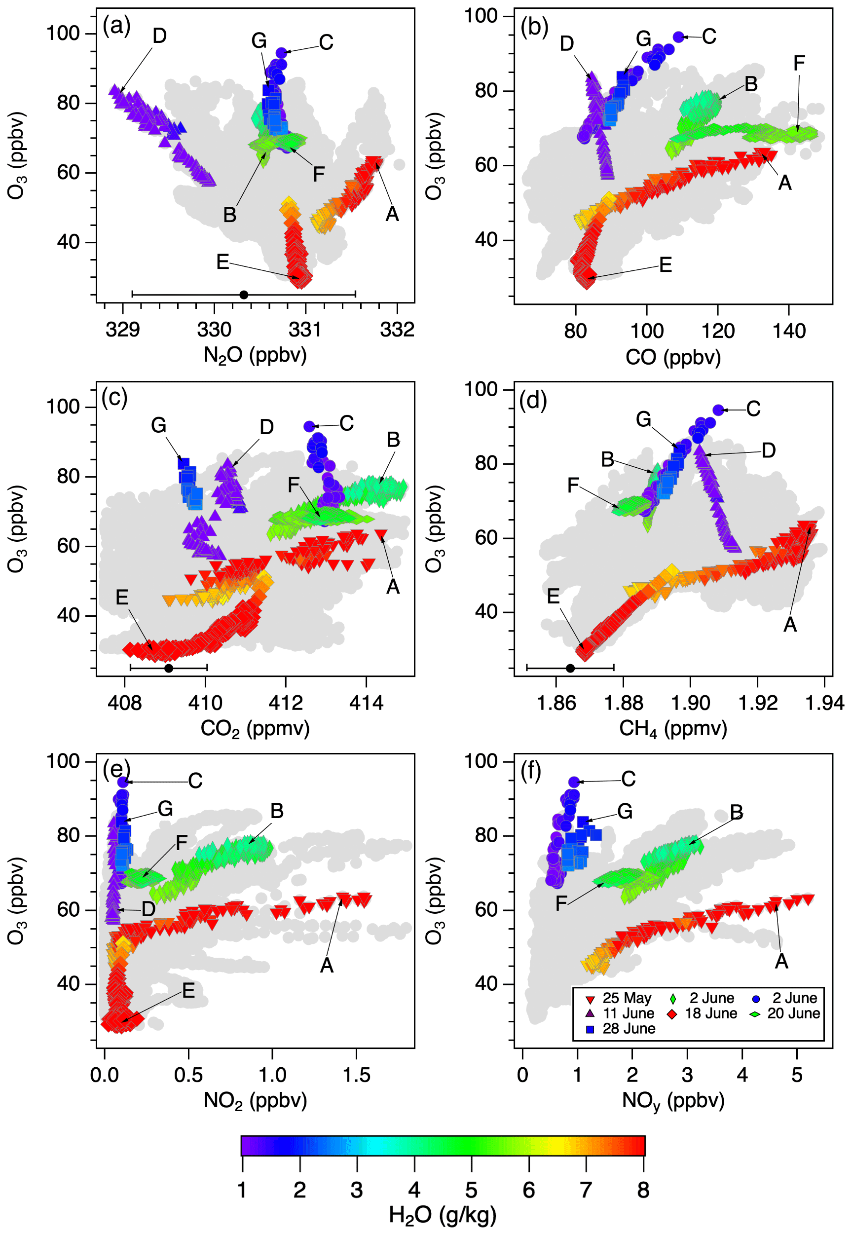
Figure 17 Scatterplots showing the relationships between O₃ and the (a) N₂O, (b) CO, (c) CO₂, (d) CH₄, (e) NO₂, and (f) NO_y tracers on AP during episodes A–G. The gray points show all of the FAST-LVOS measurements. The black points with error bars in (a), (c), and (d) represent the mean (±1σ) June 2017 concentrations from the NOAA GML Mauna Loa Observatory.

Figure 18 NOAA HYSPLIT 96 h back trajectories launched 2 km above North Las Vegas during episodes A–G. The small and large filled symbols are spaced 12 and 24 h apart, respectively. The trajectories were calculated using the 40 km NCEP Eta Data Assimilation System (EDAS) meteorology.

This interesting case illustrates yet another way that passing troughs can influence surface air quality in the LVV. Figure 18 shows that the trajectory initially followed the cyclonic circulation from L₂ (cf. Fig. 3b) southward along the California coast (hence the high moisture content) before crossing the Coast Range into the SJV on 23 May. The parcel then followed the circulation northward into the LVV as the trough moved east. The influence of the synoptic flow on the low-level winds is also seen in the transport to AP, which occurred in the early morning and several hours before the thermally forced upslope flow became established.

6.2 IOP2: 31 May–2 June

The second IOP focused on one in a series of shallow upper-level lows that spun off of the Aleutian Low in late May and early June. The MERRA-2 analysis for 06:00 UT 2 June in Fig. 3c shows the low (L₃) approaching the Pacific Northwest. A narrow filament of high-PV air emanating from the low stretches anticyclonically above the Nevada–Utah border, but the corresponding FLEXPART STTO3 distributions in the second column of Fig. 9 suggest that the intrusion was quite shallow. The ASIACO distributions in Fig. 10 show bands of Asian pollution on both sides of the stratospheric filament, with the pollution descending to at least 400 hPa above California. The TOPAZ and ozonesonde measurements in Fig. 12a show two downward-sloping bands of high O₃ between the top of the convective mixed layer and ≈ 9 km a.g.l. on the afternoon of 1 June, with the lowermost band appearing to merge with the mixed layer on the afternoon of 2 June. The backscatter curtains in Fig. 12b also show slightly higher β in the uppermost layer at 5 km a.g.l. than in the lower one at 4 km a.g.l.

The aircraft and ozonesonde profiles in Fig. 15 also show the two O₃ layers above the LVV in the morning, but the aircraft measurements show little indication of the lower layer in the profile above AP, and Fig. 16 shows it to have been rather tenuous between Las Vegas and Barstow. Figures S2 and S3 show that both layers were very dry (3 %–8 % RH), but only the uppermost layer was elevated in CH₄. This, together with the backscatter measurements in Fig. 12b, suggests that the upper layer was mostly Asian pollution, while the lower layer was mostly stratospheric. The TOPAZ curtain plot and afternoon aircraft profiles show that the convective boundary layer completely entrained the lower (stratospheric) layer and reached the bottom of the upper (Asian pollution) layer, where some entrainment must also have taken place.

The mobile laboratory measurements from AP in Figs. 6 and 17 show a pronounced O₃ peak on the afternoon of 2 June (episode B), but the other tracers show that this peak was caused by continental air and not the stratospheric intrusion or Asian pollution plume, consistent with the model-based attribution of the 2 June O₃ peak to regional pollution (Zhang et al., 2020). The sampled air had typical tropospheric N₂O concentrations and elevated CO, CO₂, NO₂, and NO_y concentrations consistent with anthropogenic pollution. The high NO₂ $/$ NO_y ratio points to local sources, and the wind barbs in Fig. 12 show that the air was transported up Kyle Canyon from the LVV by the afternoon upslope flow. The HYSPLIT trajectory in Fig. 18 (green line) approaches southern Nevada from the southeast without passing over California or any of the fires burning in Mexico and Arizona at the time. Similar local upslope events occurred frequently in late June (14, 16, 22, and 30 June) after the subtropical ridge became established.

6.3 IOP3: 10–14 June

The third IOP was triggered by another deep closed low (L₄) that moved into the western US in the second week of June. This cyclonic system was unusually deep for mid-June, and the PV plot for 12:00 UT on 12 June in Fig. 3d appears very similar to that for 00:00 UT 18 May (Fig. 3a). The cold front brought strong (> 10 m s⁻¹) south-southwesterly winds to Clark County and freezing temperatures (−5 ^∘C) to AP on the night of 11–12 June (Fig. S1). The FLEXPART STTO3 analyses in Fig. 9 show a deep cyclonic stratospheric intrusion descending to at least 700 hPa over southern Nevada, and the corresponding ASIACO analyses in Fig. 10 show cyclonic bands of pollution descending ahead of the stratospheric air. The RAQMS and RAP-Chem forecast plots in Fig. 8 appear similar.

The third IOP was extended to 5 d (10–14 June), with aircraft sorties flown on all 5 d and ozonesondes launched on 4 (10–13 June). The curtain plot in Fig. 13a shows a continuous TOPAZ run of 60 h lasting from 08:00 PDT on 11 June to 21:00 PDT on 13 June. The lidar and superimposed ozonesonde profiles show a complex network of O₃ filaments descending into the lower troposphere, with more than 150 ppbv of O₃ approaching to within 3.3 km of the surface at ≈ 03:00 PDT on 12 June and ≈ 250 ppbv measured at 5.5. km a.g.l. around 09:00 PDT. The aircraft, ozonesonde, and lidar profiles in Fig. 15 show more than 120 ppbv of O₃ between 6 and 8 km a.g.l. in the early afternoon of 12 June, and Fig. 16 shows the intrusion sloping downward to the south, with more than 140 ppbv measured along the 5.5 km a.s.l. flight leg between Barstow and Jean. The profiles near the NLVA and AP also show elevated CH₄ in the air above and below the high-O₃ layer (Fig. S4), which along with the elevated backscatter beneath the tongue in Fig. 13b shows the Asian pollution descending ahead of the stratospheric air.

Figure 13a shows that the O₃ maximum of 84 ppbv recorded around 23:00 PDT on 11 June by the mobile laboratory on AP (episode D) occurred close to the deepest penetration of the intrusion in the lidar curtain. The sampled air was extremely dry (≈ 0.1 % H₂O), and the stratospheric origin was confirmed by the low N₂O concentrations in Fig. 6 and the negative correlations of O₃ with CO, CH₄, and N₂O in Fig. 17. The NO_y converter was offline during this episode, but the NO_x concentrations were near the detection limit. Similar chemical characteristics were measured in the air sampled during the first of the two O₃ peaks that appeared on the morning of 5 June and are mentioned in Sect. 5.2. Figure 18 (purple line) shows the HYSPLIT back trajectory descending from the northwest over the previous 72 h.

Interestingly, this large intrusion did not lead to particularly high surface O₃ in the LVV on 11–13 June since the high winds from the cold front dispersed most of the locally produced O₃ and other pollutants ahead of the descending stratospheric air (Langford et al., 2012). The curtain plots do show a short-lived increase in the lowest 2 km on the afternoon of 11 June, when the surface O₃ concentrations briefly climbed from 50 to 70 ppbv at the NLVA. However, the GFDL-AM4 model suggests that the intrusion layer was mixed into regional pollution on 13–14 June and pushed the MDA8 O₃ to exceed the 70 ppbv NAAQS level at sites across the SWUS, including several sites in Clark County (Zhang et al., 2020). Once stratospheric air is mixed into local pollution, it loses its key stratospheric characteristics (e.g., low CO and low H₂O), challenging diagnosis of its surface impacts directly based on observations. This case study demonstrates the importance of integrating observational and modeling analysis for the unambiguous attribution of high-O₃ events in the SWUS (Zhang et al., 2020).

6.4 IOP4: 27–30 June

The final IOP targeted a weak trough (L₈) that crossed the Canadian border near the end of June. The MERRA-2 analysis for 06:00 UT 29 June (Fig. 3f) shows the PV maximum on the western flank of the trough. The analysis also shows the latest (L₈) in a series of cut-off lows (COLs) (Nieto et al., 2005) that formed off the coast of California in late June. These COLs typically meandered around the eastern Pacific for several days before rejoining the main flow, and Fig. 3f shows a narrow filament connecting L₉ to the remnants of L₇ (cf. Fig. 3e), which now lies above the Midwest. The FLEXPART STTO3 tracer in Fig. 9 shows both a cyclonic intrusion from L₈ descending to 500–600 hPa above Oregon and the narrow filament connecting the two COLs above southern Nevada on the 400 hPa surface. Figure 10 shows that there was significant Asian pollution between the filament and the cyclonic intrusion.

The TOPAZ curtain plot in Fig. 14 shows high (> 80 ppbv) O₃ above the boundary layer on 29 and 30 June, with up to 90 ppbv measured in the boundary layer on 30 June. The SA profiles from these days (not shown) found very dry air with depressed CH₄ concentrations in the O₃-rich layers above 4 km a.g.l., suggesting that they originated in the stratosphere. The most interesting measurements are those from 28 June, however, which show a thin layer with more than 100 ppbv of O₃ but low β disappearing into the convective mixed layer in the early afternoon, the most striking example of boundary layer entrainment observed during FAST-LVOS. The companion paper by Zhang et al. (2020) refers to this as an “unattributed event” since the layer was not resolved by either the AM4 (C192: ≈ 50 × 50 km² horizontal, ≈ 200 m vertical) or GEOS-Chem global models and cannot be resolved by FLEXPART for that matter. The spatial inhomogeneity of the layer is evidenced by the aircraft measurements in Figs. 15 and 16. Figure S3 shows that the air was very dry both within and above the mystery layer, and the combination of extreme dryness and low β rules out biomass burning or regional pollution. The layer was also rich in CH₄, suggesting that it was not a stratospheric intrusion.

Figure 14 shows that the winds on the summit of AP were mostly southerly during the morning and early afternoon of 28 June, and the mobile laboratory sampled air with much lower O₃ concentrations than that profiled by the lidar. The winds briefly rotated to the northwest in the early evening, and the mobile laboratory recorded a drop in relative humidity and increase in O₃ around 18:30 PDT (episode G). The relationships in Fig. 17 suggest that this spike was caused by Asian pollution, a conclusion supported by the HYSPLIT back trajectory (dashed blue line) in Fig. 18, which descends from the upper troposphere over the Pacific Ocean before passing over the SJV well above the boundary layer. Although the transient peak in Fig. 6 was detected more than 6 h after the O₃ layer was entrained, it does support the conclusion that Asian pollution was present in the vicinity of AP on 28 June.

7 Other transport examples

Not all of the interesting transport episodes occurred during one of the four IOPs, and the labels C, E, and F in Figs. 6, 17, and 18 highlight three other examples. Figure 6a shows that the highest 1 min O₃ concentrations (≈ 95 ppbv) measured on AP during FAST-LVOS 2017 were sampled during episode C around 02:00 PDT on the morning of 9 June. The high O₃ lasted for about an hour but occurred several hours after TOPAZ had ceased operations for the night. However, the 8 June curtain plot in Fig. 4d shows a 1 km deep layer of high O₃ just above the top of the boundary layer throughout the observing session that appears to have persisted through the night and into the next morning, when the lidar operations resumed. The unusual dryness of the air sampled on AP and relationships between O₃ and the other measured species (Fig. 17) suggest that this layer was also Asian pollution that recently descended from the upper troposphere. The episode C measurements completely overlap with the measurements from 28 June (episode G) in many of the scatterplots, suggesting a common origin. The HYSPLIT trajectories in Fig. 18 are also similar, and the peak concentrations measured by TOPAZ, ≈ 105 ppbv on 8 June and ≈ 115 ppbv on 28 June, are also comparable.

The 1 min mobile laboratory measurements from the morning of 18 June (episode E) include both the highest H₂O (12 g kg⁻¹) and lowest O₃ concentrations (29 ppbv) measured on AP during FAST-LVOS 2017. Figure 4f shows that TOPAZ also measured unusually low O₃ throughout the tropospheric column. As noted above, this episode is attributed to transport of clean marine air deep into the IMW by the anticyclonic flow around the subtropical ridge (Fig. 3e), and the HYSPLIT back trajectory (Fig. 18, dashed red line) suggests that this moist background air was lifted into the lower free troposphere above the Pacific Ocean more than 4 d earlier. Figures 6 and 17 show that the mobile laboratory also measured very low O₃, CO, CO₂, CH₄, and NO₂ concentrations on AP (the NO_y converter was offline). The filled black circles in Fig. 17 show that the O₃, N₂O, CO₂, and CH₄ concentrations measured at AP on the morning of 18 June were comparable to the mean (±1σ) June 2017 values measured at the high-elevation NOAA GML Mauna Loa Observatory (https://gml.noaa.gov/dv/data/, last access: 16 August 2021). These measurements are thought to represent the background concentrations in the free-tropospheric air reaching the US west coast.

The final example (episode F) coincides with the highest backscatter (Fig. 5f) measured above the NLVA during FAST-LVOS 2017. These measurements were made about 24 h after the start of the Holcomb Fire near Big Bear on the afternoon of 19 June (cf. Fig. 1). This fire grew rapidly but was battled aggressively, and the expansion was checked at ≈ 600 ha (≈ 1500 acres) by the evening of 21 June. The anticyclonic path followed by the HYSPLIT trajectory (dashed green line) in Fig. 18 passed directly over the Holcomb Fire and possibly over older fires in Arizona and northern Mexico. The curtain plots in Figs. 4f and 5f show that there was ≈ 85 ppbv of O₃ in the smoke that appeared at ≈ 3 km a.g.l. on the morning of 20 June but only ≈ 50 ppbv of O₃ in the denser smoke that appeared between 4 and 6 km a.g.l. in the afternoon and evening. Some of the smoke from the second plume was entrained by the convective boundary layer, and the CO time series from the mobile laboratory on AP shows a corresponding rise to more than 140 ppbv. However, Fig. 17e shows that there was little NO₂ in the second plume, which is consistent with the absence of any O₃ enhancement in either the sampled air or the lidar measurements.

8 Baseline ozone during FAST-LVOS

The top five panels of Fig. 19 show the hourly averaged and MDA8 O₃ measurements from the remote sampling sites operated by the WMRC and the NVDEP during FAST-LVOS. All of these sites are located well away from populated areas, with the WMRC located ≈ 310 km WNW of the LVV and the NVDEP monitors located between 180 and 250 km to the north (cf. Fig. 1). The bottom panel shows the measurements from the monitor maintained by the CCDAQ in the town of Mesquite ≈ 120 km NE of Las Vegas, near the Nevada–Utah border. MDA8 O₃ concentrations exceeding 65 and 70 ppbv are highlighted in orange and red, respectively. The mean MDA8 O₃ mixing ratio (±1σ, the standard deviation of the mean) is shown in each plot. These measurements show a pronounced elevation trend consistent with descent of O₃ from the free troposphere and destruction at the surface. The former is reflected in the higher mean values and episodic increases at the higher elevations and the latter in the low nighttime values at the lower elevations.

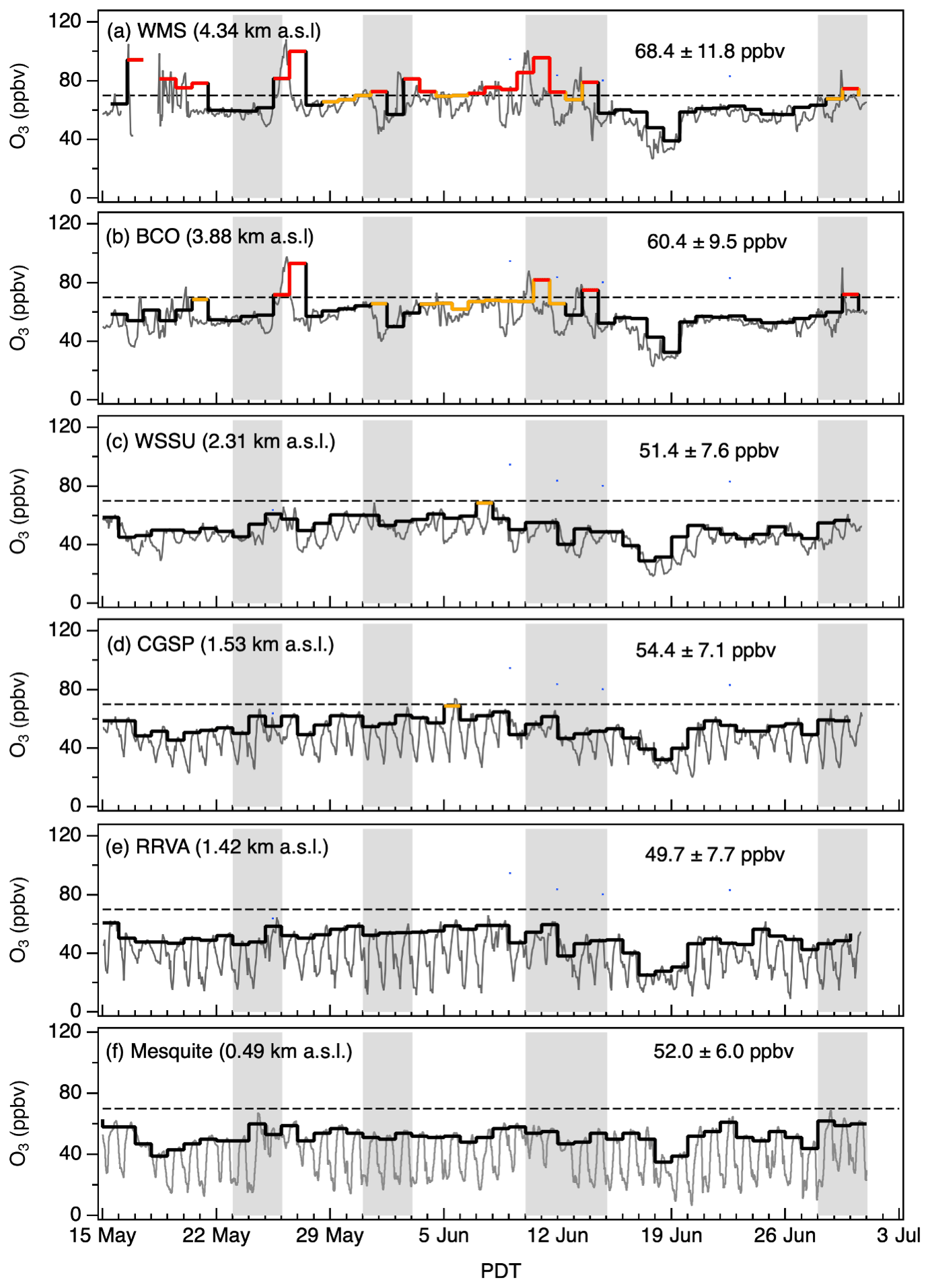
Figure 19 Time series of the 1 h average (gray line) and MDA8 O₃ (black staircase) measurements from the remote monitoring sites. The monitor elevations are shown in parentheses. (a) White Mountain Summit, (b) Barcroft Observatory, (c) Warm Springs Summit, (d) Cathedral Gorge State Park, (e) Railroad Valley, and (f) Mesquite. MDA8 O₃ concentrations exceeding the 2015 NAAQS of 70 ppbv (dashed line) and a potential NAAQS of 65 ppbv are highlighted in red and orange, respectively. The gray bands show the four IOPs. The mean concentrations (±1σ) are calculated from the 15 May to 30 June MDA8 O₃ measurements.

The WMRC operates the highest-elevation long-term O₃ monitors in the continental US, with both the WMS (4.34 km a.s.l.) and BCO (3.88 km a.s.l.) located roughly 1 km higher than the CASTNET site in Gothic, CO (2.93 km a.s.l.), which is the highest regulatory O₃ monitor in the US. The MDA8 O₃ measured at the WMS exceeded the 2015 NAAQS of 70 ppbv on 17 of the 46 FAST-LVOS sampling days, with a mean MDA8 O₃ of 68 ± 12 ppbv between 15 May and 30 June, when there were persistent O₃ layers aloft, and 73 ± 11 ppbv between 23 May and 14 June, the 22 d interval bracketing the beginning of the first and end of the third IOPs. High O₃ was measured during each of the four IOPs, with the 1 h peak concentrations exceeding 100 ppbv on 16 May, 25–26 May, and 9–10 June. The MDA8 O₃ was greater than 65 ppbv on 24 d, including 18 of the 22 d between 23 May and 14 June, and the 4MDA8 O₃ for the 6-week period was 86 ppbv. The MDA8 O₃ concentrations were similar but about 8 ppbv lower on average at the BCO.

The mean MDA8 O₃ at WSSU, the highest-elevation NVDEP site at 2.3 km a.s.l., was about 17 ppbv lower than that at WMS, with a 4MDA8 O₃ of 61 ppbv. The large episodic increases measured by the WMRC monitors during the IOPs did not reach the lower-lying NVDEP sites, and there were no NAAQS exceedances by any of these non-regulatory monitors. Nevertheless, the mean MDA8 O₃ at these three remote sites ranged from ≈ 50 to 55 ppbv, or 70 %–80 % of the NAAQS, between mid-May and the end of June, with 4MDA8 O₃ concentrations ranging from 59 to 62 ppbv (84 %–88 % of the NAAQS). An earlier analysis of springtime (March–May) measurements from 2012 and 2013 at CGSP (Fine et al., 2015a) found very similar mean MDA8 O₃ concentrations of 51 ± 6 and 50 ± 8 ppbv, respectively. These measurements are comparable to the background (i.e., formed from natural sources plus anthropogenic sources in countries outside the US) monthly mean springtime MDA8 O₃ concentration of 50 ppbv estimated by Lin et al. (2012a, b) for higher elevations in the IMW using the GFDL AM3 model for the year 2010 but are significantly higher than the mean MDA8 O₃ of 40 ± 7 ppbv derived by Zhang et al. (2011) using GEOS-Chem model runs for the years 2006–2008 and the upper limit of 40–45 ppbv for the seasonal mean MDA8 estimated by Dolwick et al. (2015) using Community Multiscale Air Quality (CMAQ) and Comprehensive Air Quality Model with Extensions (CAMx) runs for the year 2007. These differences should be viewed with caution since they do not account for changes in Asian precursor emissions or differences in trans-Pacific pollution transport and STT caused by the position of the jet stream (Lin et al., 2015; Albers et al., 2018; Breeden et al., 2021).

9 Implications for air quality attainment

The EPA has designated Las Vegas, Nevada, a marginal non-attainment area for O₃ (https://www3.epa.gov/airquality/greenbook/jnc.html, last access: 16 August 2021). The warm and sunny conditions that lead to rapid photochemical production of O₃ also drive the upslope flow into the Spring Mountains that causes O₃ and other pollutants to accumulate in the northwestern LVV. The highest O₃ concentrations are usually measured at the Joe Neal (C75) and Walter Johnson (C71) monitors (cf. Fig. 1), which had 2017 ozone design values, i.e., the 3-year running average of the fourth-highest MDA8 O₃, of 74 and 72 ppbv, respectively. Figure 20 plots the hourly averaged and MDA8 O₃ measurements from these two sites during FAST-LVOS, along with the corresponding measurements from the Apex (C22), Jean (1019), and Indian Springs (C7772) monitors (cf. Fig. 1). The thin blue line in each plot represents the average of the RRVA, CGSP, and WSSU MDA8 O₃ measurements from Fig. 19, which we use as an estimate for the southern Nevada mean baseline MDA8 O₃. The Joe Neal and Walter Johnson monitors also recorded the highest O₃ concentrations in Clark County during FAST-LVOS and exceeded the 2015 NAAQS on 7 and 6 d, respectively. Most of these exceedances coincided with the higher temperatures that followed the poleward expansion of the subtropical ridge in mid-June (cf. Fig. S1). Several of the other monitors located within a 15 km radius of the NLVA also exceeded the NAAQS on at least 1 of these days. There was only one exceedance each at the slightly more distant Apex (32 km NE) and Green Valley (22 km SE) monitors and no exceedances at the Boulder City (40 km SE), Jean (49 km SSE), or Indian Springs (58 km NW) monitors (cf. Fig. 1c). Note that the Jean monitor was offline from 9–12 June. All of the CCDAQ monitors measured unusually low O₃ on 18–19 June.

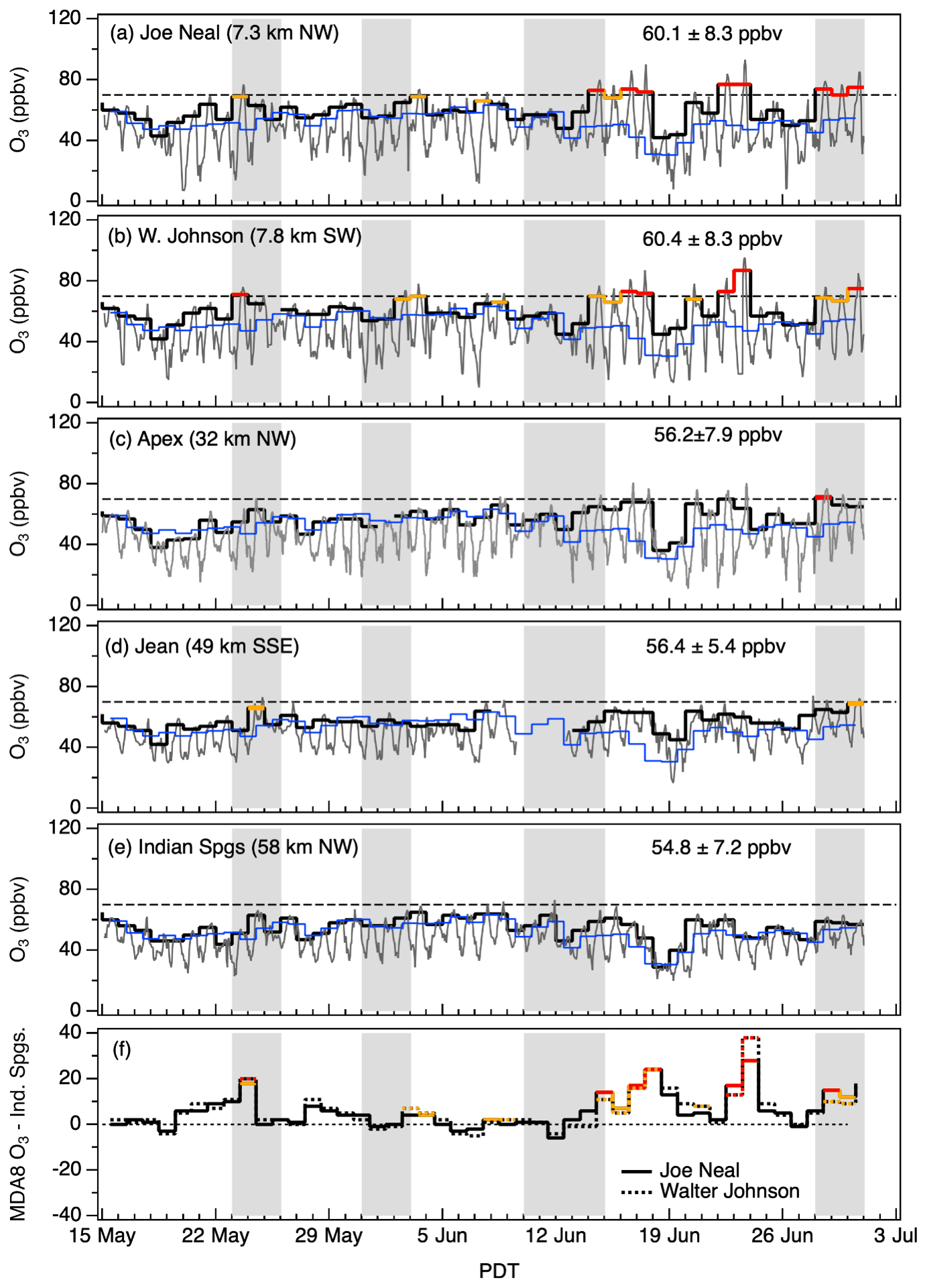
Figure 20 Time series of the 1 h (gray line) and MDA8 (black staircase) O₃ measurements from the CCDAQ (a) Joe Neal, (b) Walter Johnson, (c) JD Smith, (d) Jean, and (e) Indian Springs monitors. The distances from the NLVA are shown in parentheses. Note that the Jean monitor was offline 9–12 June. The blue lines show the baseline MDA8 O₃ estimated from the mean of the NVDEP measurements. Panel (f) plots the differences between the Indian Springs monitor and the Joe Neal (solid) and Walter Johnson (dotted) monitors. MDA8 O₃ concentrations exceeding the 2015 NAAQS of 70 ppbv (dashed line) and a potential NAAQS of 65 ppbv are highlighted in red and orange, respectively. The gray bands show the four IOPs. The mean concentrations (±1σ) are calculated from the 15 May to 30 June MDA8 measurements.

The MDA8 O₃ measured by the Indian Springs monitor was very similar to the NVDEP baseline values, with the largest differences arising on 16–17 June, when the anticyclonic marine incursion had reached the more northerly NVDEP sites but had not yet reached Clark County. The mean NVDEP and Indian Springs time series agree to within 3 % on average (R² = 0.69) if the measurements from these 2 d are excluded. This suggests that the Indian Springs measurements may be a good proxy for the LVV baseline O₃ during the FAST-LVOS campaign, and the solid black line in Fig. 20f represents the difference between the Joe Neal MDA8 O₃ concentrations and the Indian Springs monitor. The dotted line is similar but shows the difference for the Walter Johnson monitor. The measurements from days where the MDA8 O₃ concentrations exceeded 65 or 70 ppbv are highlighted as before. The MDA8 O₃ concentrations at Joe Neal and Walter Johnson were significantly higher than the baseline concentrations on 23 May, with the Walter Johnson and Joe Neal monitors reaching 71 and 69 ppbv, respectively. Although the lidar, aircraft, and ozonesonde observations showed high O₃ aloft throughout the first IOP, there was no obvious mixing of the high O₃ into the boundary layer. There were multiple exceedances in the San Joaquin Valley and South Coast air basins on 22–24 May, however, and the elevated O₃ in the LVV on 23 May is most likely due to regional transport and local production (cf. Sect. 6.1). Ozone was also elevated in the LVV on 2–3 June, and the measurements in Fig. 12 do appear to show entrainment of stratospheric O₃ and Asian pollution into the boundary layer, although this supposition could not be confirmed by the AP measurements. The MDA8 O₃ reached 68 and 65 ppbv, respectively, at Walter Johnson and Joe Neal on 2 June and 70 and 69 ppbv on 3 June. The descending O₃ may also have contributed to an isolated cluster of NAAQS exceedances at state and tribal monitors in southwestern Colorado and northwestern New Mexico and to the MDA8 O₃ of 70 ppbv recorded at Mesa Verde National Park on 3 June.

The high winds (> 20 m s⁻¹ at the surface) preceding the major intrusion event of 11–13 June (IOP3) cleared local pollution out of the LVV ahead of the descending stratospheric air, and the MDA8 O₃ concentrations at Walter Johnson and Joe Neal reached only 59 and 57 ppbv on 11 June. Interestingly, the highest reported MDA8 O₃ concentrations in Clark County on that day were 63 and 60 ppbv at Indian Springs and Apex, respectively. There were multiple NAAQS exceedances in Arizona on 13–15 June, however, including an MDA8 O₃ concentration of 91 ppbv measured on 14 June about 60 km northeast of Phoenix at the Tonto National Monument. The GFDL-AM4 model estimated 20–30 ppbv MDA8 O₃ enhancements from stratospheric influence around this site and other areas in Arizona on 14 June (see Fig. 9 in Zhang et al., 2020). The next highest values recorded at this site in 2017 were 78 ppbv on 15 June and 77 ppbv on 13 June.

The Walter Johnson and Joe Neal measurements in Fig. 20 appear qualitatively very different from the White Mountain Summit and Barcroft Observatory measurements in Fig. 19. Nearly all of the NAAQS exceedances at the high elevation sites occurred before the middle of June, when stratospheric intrusions and Asian pollution plumes appeared frequently in the middle and lower troposphere, but nearly all of the exceedances in the LVV occurred after the middle of June, when higher temperatures and stagnant conditions increased photochemical production of O₃ in the boundary layer. The high temperatures also exacerbated regional wildfires, including the Holcomb and Brian Head fires, whose plumes reached the LVV in the third week of June (cf. Figs. 4f and 5f). Note that these fires did not increase surface O₃ at the Jean, Indian Springs, or Mesquite monitors, suggesting that the smoke plumes were NO_x-limited, and significant O₃ production required additional NO_x from urban sources in the LVV (Singh et al., 2012). High O₃ was measured both in and above the boundary layer on the last 3 d of June during IOP4, with a clear example showing the entrainment of a fine-scale Asian pollution plume by the growing convective boundary layer on 28 June. This event contributed to MDA8 O₃ of 69 and 74 ppbv at Walter Johnson and Joe Neal as well as the only exceedance by the Apex monitor which measured 71 ppbv. The high-elevation WMRC monitors also measured elevated O₃ in the lower free troposphere on 29 June, and some of this O₃ may have contributed to the exceedances in the LVV on that day.

The 2013 LVOS and 2017 FAST-LVOS campaigns were conducted over the same late spring/early summer time period, but the distribution and sources of the high O₃ measured in Clark County during 2013 and 2017 were very different. The MDA8 O₃ exceeded 70 ppbv at one or more of the Clark County monitors on 17 d in May and June of 2013 but only 8 d in May and June of 2017. In 2013, 12 of the 17 exceedance days occurred before 13 June, and 9 were in May. In 2017, 7 of the 8 exceedance days occurred after 13 June, with only 1 in May. Only one of the high-O₃ events in 2017 affected more than 4 of the 12 active monitors, but 8 of the 17 high-O₃ events in 2013 affected 4 of the 11 active monitors, and 4 affected 9 or more of the CAMSs. These were the stratospheric intrusion and wildfire event of 4–5 May (Langford et al., 2015a), stratospheric intrusion events of 21 and 25 May (Langford et al., 2018), and Asian pollution event of 21 June (Langford et al., 2017). These major events affected monitors outside of Las Vegas as well as those in the valley, and the Jean monitor exceeded 70 ppbv on 8 d in 2013 but not once in 2017 (the Indian Springs monitor was not installed until 2015).

10 Summary and conclusions

The 6-week-long FAST-LVOS field campaign collected a wealth of lidar, surface, aircraft, and ozonesonde measurements that greatly improve our understanding of O₃ transport in Clark County, Nevada, and the greater southwestern US and Intermountain West in late spring and early summer. Daily lidar observations found high-O₃ layers in the lower and middle free troposphere above Las Vegas on more than 75 % (35 of 45) of the measurement days. The highest tropospheric concentrations were measured on 11–12 June, when both the lidar and an ozonesonde launched nearby found up to 250 ppbv within 5.5 km of the surface. Several of these elevated O₃ layers were also sampled by a high-elevation research monitor located more than 300 km to the west-northwest, in the White Mountains of California (Burley and Bytnerowicz, 2011), and the MDA8 O₃ concentrations at this site averaged more than 68 ppbv over the course of the study. Simulations from the FLEXPART, GEOS-Chem, and AM4 models (Zhang et al., 2020) show that the elevated layers were created by stratospheric intrusions or long-range transport from Asia and, in most cases, a mixture of the two. Aircraft measurements made during the four IOPs support this conclusion, and the aircraft mapped the spatial distribution of these plumes above the Mojave Desert in southern Nevada and California. FAST-LVOS also documented several fine-scale anticyclonic streamers in addition to the deep cyclonic intrusions that are the focus of most studies.

The FAST-LVOS measurements also captured several examples of O₃ being entrained from aloft by the convective boundary layer, and correlations between the different tracers measured on AP (2.7 km a.s.l.) showed the distinctive signatures of both stratospheric air and Asian pollution on multiple occasions. The AP measurements also found wildfire influences and evidence for regional transport of anthropogenic pollution from the San Joaquin Valley in addition to local upslope transport of pollution from the LVV. Although none of the stratospheric intrusions or Asian pollution events directly caused any of the NAAQS exceedances in the LVV during FAST-LVOS, they clearly added to the surface concentrations on at least 1 (14 June) of the exceedance days and contributed to the mean MDA8 O₃ of 50–55 ppbv measured at the remote sites in rural Nevada during the study. These mean baseline concentrations represent 70 %–80 % of the 2015 NAAQS of 70 ppbv, making it more difficult for western air quality managers to maintain surface O₃ concentrations below the NAAQS in the IMW during late spring and early summer (Cooper et al., 2015; Uhl and Moore, 2018).