Mixing layer transport flux of particulate matter in Beijing, China

Quantifying the transport flux (TF) of atmospheric pollutants plays an important role in understanding the causes of air pollution and in making decisions regarding the prevention and control of regional air pollution. In this study, the mixing layer height (MLH) and wind profile were measured by a ceilometer and Doppler wind radar, respectively, and the characteristics of the atmospheric dilution capability were analyzed using these two datasets. The ventilation coefficient (VC) appears to be the highest in the spring (3940±2110 m² s⁻¹) and lower in the summer (2953±1322 m² s⁻¹), autumn (2580±1601 m² s⁻¹) and winter (2913±3323 m² s⁻¹). Combined with the backscatter measured by the ceilometer, vertical profiles of the PM_2.5 concentration were obtained and the PM_2.5 TF in the mixing layer was calculated. The TF was the highest in the spring at 4.33±0.69 mg m⁻¹ s⁻¹ and lower in the summer, autumn and winter, when the TF values were 2.27±0.42, 2.39±0.45 and 2.89±0.49 mg m⁻¹ s⁻¹, respectively. Air pollutants transport mainly occurs between 14:00 and 18:00 LT. The TF was large in the pollution transition period (spring: 5.50±4.83 mg m⁻¹ s⁻¹; summer: 3.94±2.36 mg m⁻¹ s⁻¹; autumn: 3.72±2.86 mg m⁻¹ s⁻¹; winter: 4.45±4.40 mg m⁻¹ s⁻¹) and decreased during the heavy pollution period (spring: 4.69±4.84 mg m⁻¹ s⁻¹; summer: 3.39±1.77 mg m⁻¹ s⁻¹; autumn: 3.01±2.40 mg m⁻¹ s⁻¹; winter: 3.25±2.77 mg m⁻¹ s⁻¹). Our results indicate that the influence of the air pollutants transport in the southern regions should receive more focus in the transition period of pollution, while local emissions should receive more focus in the heavy pollution period.

1 Introduction

With the rapid development of its economy and industry, as well as its unique local topography, Beijing has become one of the cities in the world that is most seriously affected by air pollution. As early as before the 2008 Olympic Games, to fulfill the promise of a “Green Olympics”, Beijing's industries were relocated to surrounding provinces and cities. After the Olympic Games, with the promulgation of the “Action Plan for Prevention and Control of Air Pollution”, Beijing implemented a series of measures to reduce pollutants, such as raising the emission standards of motor vehicles and fuel standards for vehicles, changing coal to natural gas, changing coal to electricity and so on. These measures have gradually improved Beijing's air quality, with the annual average fine particulate matter (PM_2.5) concentration decreasing from 90 µg m⁻³ in 2013 to 58 µg m⁻³ in 2017 (Cheng et al., 2019).

Although the Beijing government has been committed in recent years to taking measures that could ensure a steady improvement in the air quality, there is still great pressure to achieve a continuous decline in the particulate matter concentration. Beijing is in the north of the North China Plain, with the southern side and the western side being surrounded by the Yan Mountains and the Taihang Mountains, respectively. Affected by the mountains to the northwest, there are more subsiding airflows, a lower mixing layer height and an extremely limited atmospheric dilution capability. In addition, pollutants tend to accumulate in front of the mountains due to the influence of southerly winds and the mountain obstructions. In central and northern China, the increase in PM_2.5 during the winter is closely related to the adverse atmospheric dilution conditions (Wang et al., 2016). Therefore, in addition to the primary emissions and secondary formation, the weak atmospheric dilution capability is also an important factor leading to the frequent occurrence of serious air pollution in Beijing.

In recent decades, the mixing layer height (MLH) and wind speed (WS) have been two major factors leading to the annual increases in the aerosol concentration and polluted days during the winter in China (Yang et al., 2016). The low MLH and low WS are also important characteristics of the weak atmospheric dilution capability (Huang et al., 2018; Liu et al., 2018; Song et al., 2014; Tang et al., 2015). The change in the MLH represents the vertical dilution capability of pollutants, and the change in the WS represents the horizontal dilution capability of pollutants. The ventilation coefficient (VC) is usually used to evaluate the vertical and horizontal dilution capability of the atmosphere (Nair et al., 2007; Tang et al., 2015; Zhu et al., 2018). Thus, it is a good choice to use the VC to evaluate the relationship between the atmospheric dilution capability and air pollution in Beijing. Although previous studies have analyzed the relationship between the MLH and pollutants (Geiß et al., 2017; Miao and Liu, 2019; Schäfer et al., 2006; Su et al., 2018), studies on the effects of the VC on the particle concentration have been extremely rare.

Although the problem of heavy pollution in northern China has improved in recent years, regional pollution problems remain, especially in the Beijing–Tianjin–Hebei region (Shen et al., 2019). There are three main transport routes affecting Beijing: the northwestern path, the southwestern path and the southeastern path (Chang et al., 2018; Li et al., 2018; Zhang et al., 2018). The occurrence of heavy pollution in Beijing is closely related to the transport of pollutants in the southern regions, mainly in southern Hebei, northern Henan and western Shandong, while the high-speed northwestern air mass is conducive to the removal of pollutants from Beijing (Li et al., 2018; Ouyang et al., 2019; Zhang et al., 2018, 2017). In recent years, the contribution of regional transport to Beijing has been increasing annually, with a trend of 1.2 % yr⁻¹, which reached 31 %–73 % in the summer and 27 %–59 % in the winter (Chang et al., 2018; Cheng et al., 2018; Wang et al., 2015). High PM_2.5 concentrations are usually accompanied by high transport flux (TF) within a day in Beijing. As pollution worsens, the contribution of the surrounding areas to the PM_2.5 in Beijing rose from 52 % to 65 % per month on average in 2016 (Zhang et al., 2018). However, during heavy pollution, the TF decreases in Beijing (Chang et al., 2018; Tang et al., 2015; Zhu et al., 2016).

To solve the regional pollution problem, joint prevention and control have been recommended for a long time. Many studies on regional transport have been carried out, but most observational studies cannot easily quantify the TF due to the lack of particle and wind vertical profiles, and it is still unclear when we need to control the emission sources and in which areas. To solve the above problems, we conducted 2 years of continuous observations on MLH and wind profiles in the Beijing mixing layer and analyzed the mixing layer dilution capability of the atmosphere. Afterwards, using the backscattering coefficient profile, we obtained the vertical PM_2.5 concentration profiles and calculated the TF profile and mixing layer TF. Finally, using the near-surface PM_2.5 concentration as an indicator to classify the air pollution degree, we analyzed the TF during the transitional and heavily polluted periods in Beijing and illuminated the main controlling factors.

2 Methods

2.1 Observational station

To understand the dilution capability characteristics in Beijing, 2 years of observations were conducted (1 January 2016–31 December 2017). The observational site is at the Institute of Atmospheric Physics of the Chinese Academy of Sciences, located west of the Jiande Bridge in the Haidian district, Beijing (39.98^∘ N, 116.38^∘ W). The northern and southern sides of the station are the northern Third and northern Fourth Ring Roads, respectively, and the eastern side is the Beijing–Tibet Expressway. The altitude (a.s.l.) is approximately 60 m. There is no obvious emission source around the observational site except for motor vehicles.

2.2 Observations of MLH and wind profiles

To analyze the dilution capability, the MLH was observed by a single-lens ceilometer (CL51, Vaisala, Finland), and the wind profile was simultaneously observed by a Doppler wind radar (Windcube 100S, Leosphere, France).

A single-lens ceilometer measures the attenuated backscatter coefficient profile of the atmosphere by pulsed diode laser lidar technology (910 nm waveband) within a 7.7 km range and determines the MLH through the positions of abrupt changes in the backscattering coefficient profile. In the actual measurement, the measurement interval was 16 s, and the measurement resolution was 10 m. More detailed descriptions are presented in the published literature (Tang et al., 2016; Zhu et al., 2016). In this study, the gradient method (Steyn et al., 1999) is used to determine the MLH; that is, the top of the mixing layer was determined by the maximum negative gradient value in the profile of the atmosphere backscattering coefficient. Moreover, to eliminate the interference of the aerosol layer structure and the detection noise, the MLH was calculated by the improved gradient method after smoothly averaging the profile data (Münkel et al., 2007; Tang et al., 2015).

Doppler wind radar uses the remote sensing method of laser detection and ranging technology and measures the Doppler frequency shift generated by the laser through the backscatter echo signal of particles in the air. The Windcube 100S can provide 3-D wind field data within a 3 km range of the system, including u, v and w vectors. In the actual measurement, starting from 100 m, the spatial resolution is 50 m, the WS accuracy is < 0.5 m s⁻¹ and the radial WS range is −30 to 30 m s⁻¹.

2.3 Other data

During the observations, the hourly PM_2.5 concentrations of the Beijing Olympic Sports Centre (39.99^∘ N, 116.40^∘ W) were obtained from the Ministry of Ecology and Environment of China (http://www.mee.gov.cn/, last access: 22 July 2019).

2.4 Analytical method

The atmospheric dilution is composed of vertical and horizontal dilution, which can be characterized by the MLH and wind speed in the mixing layer (WS_ML), respectively. The VC (m² s⁻¹) was obtained by combining the MLH (m) and WS_ML (m s⁻¹) and can be used for a comprehensive evaluation of the vertical and horizontal dilutions. Higher dilution-related parameters (MLH, WS_ML and VC) indicate a stronger dilution capability, which is conducive to the transport and dilution of heavy air pollution.

The VC calculation method is as follows:

$$\begin{array}{}\text{(1)}& {\displaystyle }& {\displaystyle }\text{VC}=H_{\text{ML}}\times {\text{WS}}_{\text{ML}},\text{(2)}& {\displaystyle }& {\displaystyle }{\text{WS}}_{\text{ML}}={\displaystyle \frac{\mathrm{1}}{n}}{\sum }_{i=\mathrm{1}}^n{\text{WS}}_i,\text{(3)}& {\displaystyle }& {\displaystyle }{\text{WS}}_i=\sqrt{\stackrel{\mathrm{‾}}{{\mathit{u}}_i^{\mathrm{2}}}+\stackrel{\mathrm{‾}}{{\mathit{v}}_i^{\mathrm{2}}}},\end{array}$$

where WS_ML is the average WS within the mixing layer, calculated by Eq. (2), H_ML is the height of the mixing layer, WS_i is the WS observed at a certain height, calculated by u_i and v_i in the wind profile according to Eq. (3), and n is the number of measurement layers in the mixing layer (Nair et al., 2007).

The TF (mg m⁻² s⁻¹) is determined by the WS and the PM_2.5 concentration in the area under analysis. The calculation method for a certain height is shown in Eq. (4):

$$\begin{array}{}\text{(4)}& {\text{TF}}_{u_i}={\mathit{u}}_i\times C_i,\end{array}$$

where C_i is the concentration of PM_2.5 at a certain height. However, it is extremely difficult to observe the vertical PM_2.5 concentration in the mixing layer. To obtain the PM_2.5 concentration profile, we studied the backscattering coefficient measured by the ceilometer and found that the concentration of near-surface PM_2.5 is strongly correlated with the backscattering coefficient at 100 m (Fig. S1). Thus, based on the relationship between the two, the backscattering coefficient profile can be used to invert the vertical PM_2.5 concentration profile. Then, the TFs in the mixing layer are calculated as follows:

$$\begin{array}{}\text{(5)}& \begin{array}{rl}& {\text{TF}}_u=\underset{i=\mathrm{1}}{\overset{n}{\int }}({\mathit{u}}_i\times C_i),\\ & {\text{TF}}_v=\underset{i=\mathrm{1}}{\overset{n}{\int }}({\mathit{v}}_i\times C_i).\end{array}\end{array}$$

Through the above method, radial and zonal TFs can be obtained, and vector synthesis in two directions can be conducted to obtain the main transport direction to find the transport source area.

3 Results and discussion

3.1 Boundary layer meteorology

3.1.1 Seasonal variation

To understand the variations in the atmospheric dilution capability, we carried out continuous measurements of the MLH and wind profile within the mixing layer over a 2-year period (1 January 2016–31 December 2017). The availability was verified after MLH elimination by Tang et al. (2016). After the exclusion of the data of the MLH under rainy, sandstorm and windy conditions, the data availability was 95 % over the 2-year period, higher than that of previous studies (Mues et al., 2017; Tang et al., 2016). The availability was the lowest in February, at 86 %, and the highest in July, at 99 %.

In terms of the seasonal variation, the average MLHs for the spring (781±229 m; value ± standard deviation) and summer (767±219 m) were higher than those of the autumn (612±166 m) and winter (584±221 m; Fig. 1). However, WS_ML was different from the MLH in terms of the seasonal variation, with the largest value being 4.6±1.6 m s⁻¹ in the spring, followed by the winter (4.1±2.7 m s⁻¹) and autumn (3.7±1.6 m s⁻¹), and the smallest value being 3.6±1.1 m s⁻¹ in the summer. The VC was calculated by the MLH and wind profile, and the results demonstrate that the dilution capability was strongest in the spring, as the VC reached as high as 3940±2110 m² s⁻¹. The atmospheric dilution capabilities for the summer, winter and autumn were similar, with VC values of 2953±1322, 2913±3323 and 2580±1601 m² s⁻¹, respectively. A monthly analysis shows that the atmospheric dilution capability was strongest in May, when the VC was as high as 5161±2085 m² s⁻¹, and worst in December, when the VC was only 1690±1072 m² s⁻¹. The VC value in May was 3.1 times that in December. To analyze the impact of the dilution capacity on PM_2.5, the seasonal variation in PM_2.5 was analyzed. The average PM_2.5 concentration for the winter (80±87 µg m⁻³) was the highest, followed by autumn (68±54 µg m⁻³) and spring (67±60 µg m⁻³), and that of the summer (51±29 µg m⁻³) was the lowest. The lowest monthly average PM_2.5 concentration was 42±26 µg m⁻³ in August. The highest monthly average was in January at 94±100 µg m⁻³, 2.2 times that in August (Fig. 1).

Figure 1 Monthly variations in mixing layer height (MLH), the wind speed in the mixing layer (WS_ML), the ventilation coefficient (VC) and PM_2.5 in Beijing.

Although there is little difference in the dilution capability between the summer, autumn and winter, there is serious pollution in the autumn and winter. To analyze this problem, the VC frequency distribution was studied. The results show that the VC had a high frequency in the range of 1000–4000 m² s⁻¹ from 2016 to 2017, but the frequency distribution was different in different seasons (Fig. 2). The VC showed a strong dilution capability in the spring, mainly in the range of 2000–5000 m² s⁻¹, with the highest frequency (24 %) in the range of 2000–3000 m² s⁻¹. In the summer, the high frequency of the VC occurred in the range of 1000–4000 m² s⁻¹, which was slightly lower than that in the spring, and the highest frequency (27 %) occurred in the range of 3000–4000 m² s⁻¹. Additionally, the VC high frequency appeared in lower ranges in the autumn and winter. The VC occurred at a high frequency of 1000–3000 m² s⁻¹ in the autumn, and the highest frequency occurred within the range of 2000–3000 m² s⁻¹, accounting for 33 %. In the winter, the VC appeared more frequently in the range of 0–2000 m² s⁻¹ and was the highest in the range of 1000–2000 m² s⁻¹, which was 28 %. In the winter, when the Siberian High transits, strong northwestern winds prevail in the Beijing area (Fig. 5), resulting in the higher frequency of the VC in the range of 1000–2000 m² s⁻¹. The VC frequency of 0–1000 m² s⁻¹ in the winter was significantly higher than that of the other seasons, being up to 22 %, which was 7 times that in the spring, 5 times that in the summer and 2 times that in the autumn. According to the seasonal variation in the PM_2.5 concentration, heavy pollution in the autumn and winter is related to the high frequency of poor atmospheric dilution capability.

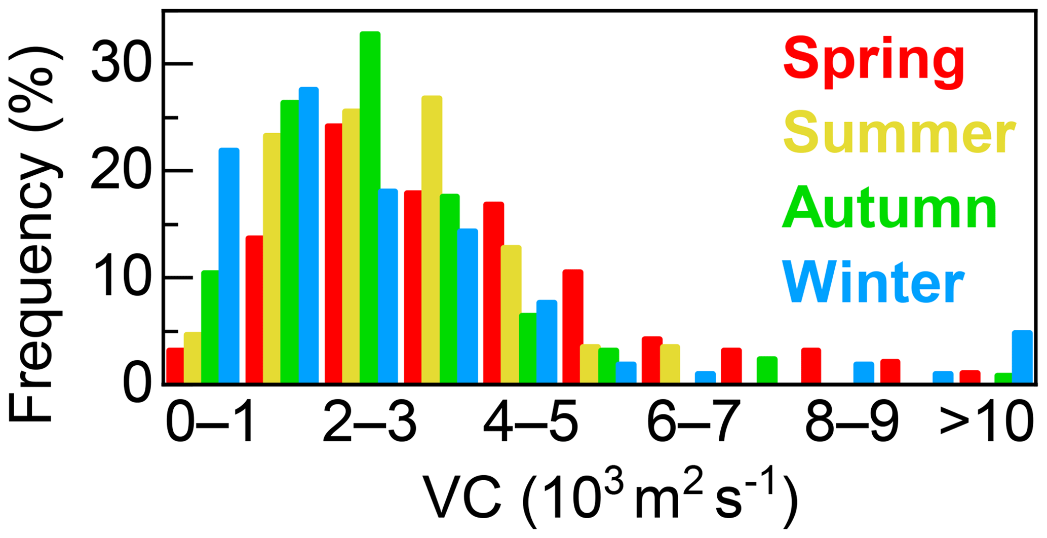
Figure 2 Frequency distribution of the daily VC from January 2016 to December 2017 in Beijing.

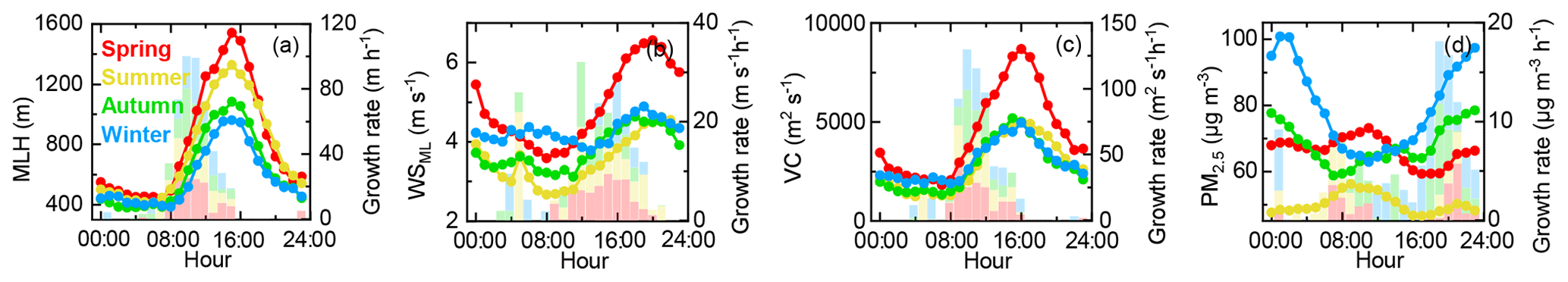
Figure 3 Diurnal variations and growth rates of MLH (a), WS_ML (b), VC (c) and PM_2.5 (d) in the spring, summer, autumn and winter in Beijing. Diurnal variations are represented by lines and scatters. Growth rates are represented by columns, and only positive values are shown in the figure.

3.1.2 Diurnal variation

Moreover, the diurnal variations in the dilution-related parameters during different seasons were analyzed to reveal the diurnal evolution of the atmospheric dilution capability. The peak and trough values of the MLH and VC appeared simultaneously at approximately 15:30 and 05:30 LT, respectively. Generally, the daily variation in the MLH is characterized by a low value at night, which increases rapidly after sunrise and reaches the maximum value in the afternoon (Fig. 3a). The daily maximum value of the MLH is seasonal, where it is higher in the spring and summer and lower in the autumn and winter. The daily minimum value of the MLH generally occurs when the mixing layer is stable and is closely related to the WS. The diurnal variation in WS_ML is smaller, with a peak at approximately 19:30 LT and a trough at approximately 10:00 LT, which are ∼ 4 h later than the peak and trough of the MLH (Fig. 3b). The diurnal variation in the VC is similar to that of the MLH, showing that the dilution capability is strong before sunset, gradually weakens after sunset and remains stable at night. The dilution capability in the spring was significantly stronger than that during the other seasons and the maximum daily value reached 8678 m² s⁻¹ (Fig. 3c). The daily maximum values of the VC in the summer, autumn and winter were close, at approximately 5000 m² s⁻¹ (Fig. 3c). The VC growth rate in the spring was significantly higher than that in the other seasons, reaching a maximum at approximately 09:00 LT. In the autumn, the VC growth rate peaked at approximately 10:00 LT, and those in the summer and winter peaked at approximately 11:00 LT. Throughout the year, the VC began to increase during the winter later than in other seasons, at approximately 09:00 LT, indicating that the weaker dilution capability remained for a longer period during the winter. The VC was weakened most rapidly in the spring; however, it was still higher than that of the other seasons after declining. In addition to the spring, the VC in the autumn and winter weakened the most rapidly and the most slowly in the summer. In general, the vertical and horizontal dilutions are strong in the spring during both the day and night. In the winter, the vertical dilution is weak during the day, and the horizontal dilution during the night is the main component. In the summer, the vertical dilution during the day is dominant.

Notable differences are present when we compare the dilution-related parameters to the PM_2.5 concentration. The daily maximum PM_2.5 concentrations in the spring, summer, autumn and winter were 73 µg m⁻³ (11:00 LT), 56 µg m⁻³ (09:00 LT), 78 µg m⁻³ (23:00 LT) and 101 µg m⁻³ (01:00 LT), respectively. The differences between the maximum and minimum were 14, 10, 20 and 38 µg m⁻³, respectively. Thus, the diurnal variation in PM_2.5 can be divided into two categories: (1) the highest value occurs in the midday in the spring and summer, and the overall change is small, and (2) the highest value occurs during the night in the autumn and winter and differs greatly from the lowest value (Fig. 3d). The main causes of air pollution are local emissions and regional transportation. Thus, these results indicate that there are greater local contributions in the autumn and winter and higher regional transport in the spring and summer.

Figure 4 Seasonal variations in the mixing layer TF of PM_2.5 and the transport direction.

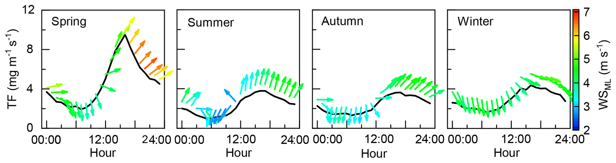
Figure 5 Diurnal variations in the mixing layer TF of PM_2.5 and transport direction during different seasons in Beijing.

3.2 Mixing layer TF of PM_2.5

3.2.1 Temporal evolution of TF

To quantify the transport of PM_2.5 in Beijing, the transport direction of PM_2.5 was characterized by the average wind direction in the mixing layer. As shown in Fig. 4, the mixing layer TF in the spring was the largest, reaching 4.33±0.69 mg m⁻¹ s⁻¹, and there was no significant difference in the summer, autumn or winter, when the TF values were 2.27±0.42, 2.39±0.45 and 2.89±0.49 mg m⁻¹ s⁻¹, respectively. The transport sources of the cold period in Beijing were predominantly from the northwesterly and westerly directions. With temperature warming, the transport direction gradually changed from west to south, mainly being southwesterly in the spring and southerly in the summer. The monthly average maximum value of the TF occurred in May, being as high as 5.00±5.21 mg m⁻¹ s⁻¹, and mainly originated from the southwestern direction, accompanied by a strong wind. The minimum value appeared in August, being as low as 1.70±1.73 mg m⁻¹ s⁻¹, which was mainly transported from western regions, with a small WS. The TF in May was 3 times that in August (Fig. 4). Therefore, the change in the transport direction leads to an obvious seasonal variation in the TF. Overall, the regional transport contributes the most to the PM_2.5 concentration in the spring, which is mainly related to increased dust activities. Regional transport has a smaller contribution in the winter, but there is a high near-surface PM_2.5 concentration, which indicates that more focus should be given to local emission source control; in the summer and autumn, the southwestern airflow transport influence on the Beijing should receive more focus.

To understand the regional transport influence on the Beijing area, the diurnal variations in the mixing layer TF were analyzed during different seasons in Beijing. The daily minimum value of the TF appeared at approximately 07:00 LT and was accompanied by a northerly wind. As the average wind direction in the mixing layer gradually turned south, the daily minimum value of the TF continued to rise until the daily maximum value appeared at approximately 16:00 LT (Fig. 5). Transport mainly occurred between 14:00 and 18:00 LT, which was consistent with the results of a previous study (Ge et al., 2018). In the spring, the WS was the highest, so the peak TF duration was the shortest; it peaked at only 16:00 LT (9.50 mg m⁻¹ s⁻¹) and then dropped sharply to 1.94 mg m⁻¹ s⁻¹. Therefore, the diurnal variation in the TF during the spring showed the characteristics of a rapid rise and rapid decline. The peak duration was approximately 3 h for a long time in the summer and autumn, where the daily maximum values were 3.79 and 3.63 mg m⁻¹ s⁻¹ and the minimum values were 1.00 and 1.30 mg m⁻¹ s⁻¹, respectively. The diurnal variation in the TF during the summer and autumn showed the characteristics of a slow rise and slow decline. Specifically, the daily variation had a strong fluctuation in the winter; peaked three times, at 14:00 LT (4.06 mg m⁻¹ s⁻¹), 16:00 LT (4.38 mg m⁻¹ s⁻¹) and 19:00 LT (4.07 mg m⁻¹ s⁻¹); then dropped slowly to 1.66 mg m⁻¹ s⁻¹. Another special point is that in the spring, summer and autumn, a high TF corresponds to a southerly wind, while in the winter, the southerly wind does not appear in the whole transport process; instead, there is a westerly wind, which is influenced by the Siberian High.

Even so, the TF variation patterns can be summarized in that a high TF corresponds to a southerly wind and a low TF corresponds to a northerly wind (Fig. 5). When the average wind direction in the mixing layer changes from north to south, the TF gradually increases from the daily minimum to the daily maximum. The TF increased by 5 times in the spring, 4 times in the summer, and 3 times in the autumn and winter. The current pattern is because areas located in the south of Beijing are heavily polluted and southerly winds help transport pollutants into the city, leading to high TFs in the afternoons (Fig. 5). However, due to the high mixing layer in the spring, the concentration of near-surface PM_2.5 did not increase. The results further confirm the conclusion that the northwestern wind in Beijing is a clean wind (Wang et al., 2015; Zhang et al., 2018). Thus, the northwestern wind is conducive to the outward transport of pollutants from Beijing, which helps in alleviating pollution. As a result, there was no high TF in the winter when the northwestern wind prevailed. On the other hand, southerly winds are stronger than northerly winds (Fig. 5), which can also result in a high TF. Therefore, the level of the TF is determined by two factors, the WS and PM_2.5 concentration. In the spring, summer and autumn, a strong southern wind prevails in the afternoon. As the southern wind is often accompanied by high PM_2.5 concentrations (Fig. S2), the TF is high. In the winter, the whole day is dominated by westerly and northerly winds. Although the northerly winds are strong, the TF is not high due to the low PM_2.5 concentration. Generally, a high WS means fast mixing, and the corresponding MLH is also high. At this time, the TF is mainly controlled by the WS. While the WS is low, the mixing speed is slow and the MLH is low. At this time, the TF is mainly controlled by PM_2.5 concentration. From the above analysis, it can be inferred that if the MLH and WS gradually decrease with the worsening of the pollution, the mixing layer TF is controlled by the WS first and then by the PM_2.5 concentration, and a maximum TF may occur at a critical moment. This moment is neither the moment of the maximum WS nor the moment of the maximum PM_2.5 concentration but rather should be somewhere in between. This will be discussed in more detail in Sect. 3.3.

Figure 6 Vertical profiles of WS (a), PM_2.5 (b) and TF of PM_2.5 (c) in different seasons in Beijing.

3.2.2 Vertical evolution of TF

After the aforementioned analyses, the transport period is known. To further explore the height of transport, we studied the seasonal variation in the TF profile in combination with the vertical wind and PM_2.5 profiles. With the increasing altitude, the WS first increases sharply at approximately 200 m and then slowly increases, and the differences between different seasons gradually become significant (Fig. 6a). The WS is always smallest in the summer and strongest in the winter. It is the same in the spring and autumn at 1200 m. Above 1200 m, the WS in the autumn exceeds that in the spring. The PM_2.5 concentration at 100 m obtained by inversion is highest in the winter (93.7 mg m⁻² s⁻¹), similar in the spring and autumn (80.3 and 75.8 mg m⁻² s⁻¹, respectively), and lowest in the summer (53.5 mg m⁻² s⁻¹; Fig. 6b). This finding is consistent with the near-surface results. Below 200 m, the PM_2.5 concentration is relatively uniform. As the height increases, the PM_2.5 concentration decreases gradually. Between 200 and 600 m, the PM_2.5 concentration begins to decrease rapidly, but the rate of decline is obviously different in different seasons. In the autumn and winter, the reduction rate of the PM_2.5 concentration is significantly higher than that in the spring and summer. As a result, the spring PM_2.5 concentration at 400 m begins to be greater than that in the winter; the summer PM_2.5 concentration at 650 m begins to be greater than that in the autumn and is at the same level as that in the winter. Over 600 m, there is no significant difference in the PM_2.5 concentration between different seasons, while the WS varies greatly. Therefore, the TF is greatly affected by the WS at high altitudes, and it is greatly influenced by the PM_2.5 concentration near the ground. The TF in the mixing layer is also affected by the MLH.

The vertical evolution of the TF is different from both the evolution of the WS and PM_2.5 concentration, and the seasonal variation remains consistent from the near-surface to the upper air. The TF for the spring is the highest, followed by the winter and autumn, and that of the summer is the lowest (Fig. 6c). The vertical variation in the TF increases first and then decreases, and a peak appears at approximately 300 m, with a value of 0.38 mg m⁻² s⁻¹ in the spring, 0.19 mg m⁻² s⁻¹ in the summer, 0.24 mg m⁻² s⁻¹ in the autumn and 0.31 mg m⁻² s⁻¹ in the winter. In the process of the TF lowering, it has different performances in different seasons. In the spring, the decline slows down at approximately 1500 m. The changes in the summer and autumn are similar. After the peak, the TF drops rapidly in the summer and autumn. The decrease rate above 500 m becomes slow and slows down again after 1500 m, and finally the profiles become vertical. In the winter, the TF declines rapidly, followed by fluctuations at approximately 1000 m. The above results preliminarily indicate that the transport mainly occurs within 200–1500 m, which will be evaluated in Sect. 3.3. To sum up, in the autumn and winter, the high concentration of PM_2.5 is concentrated near the ground, while the TF is not large, again indicating that local emissions are the main source of PM_2.5 in the autumn and winter; in the spring, affected by high-altitude transport, the PM_2.5 concentration is high; and in the summer, both the TF and PM_2.5 concentrations are at their lowest levels, indicating that regional transport may play an important role in the PM_2.5 concentration in the summer.

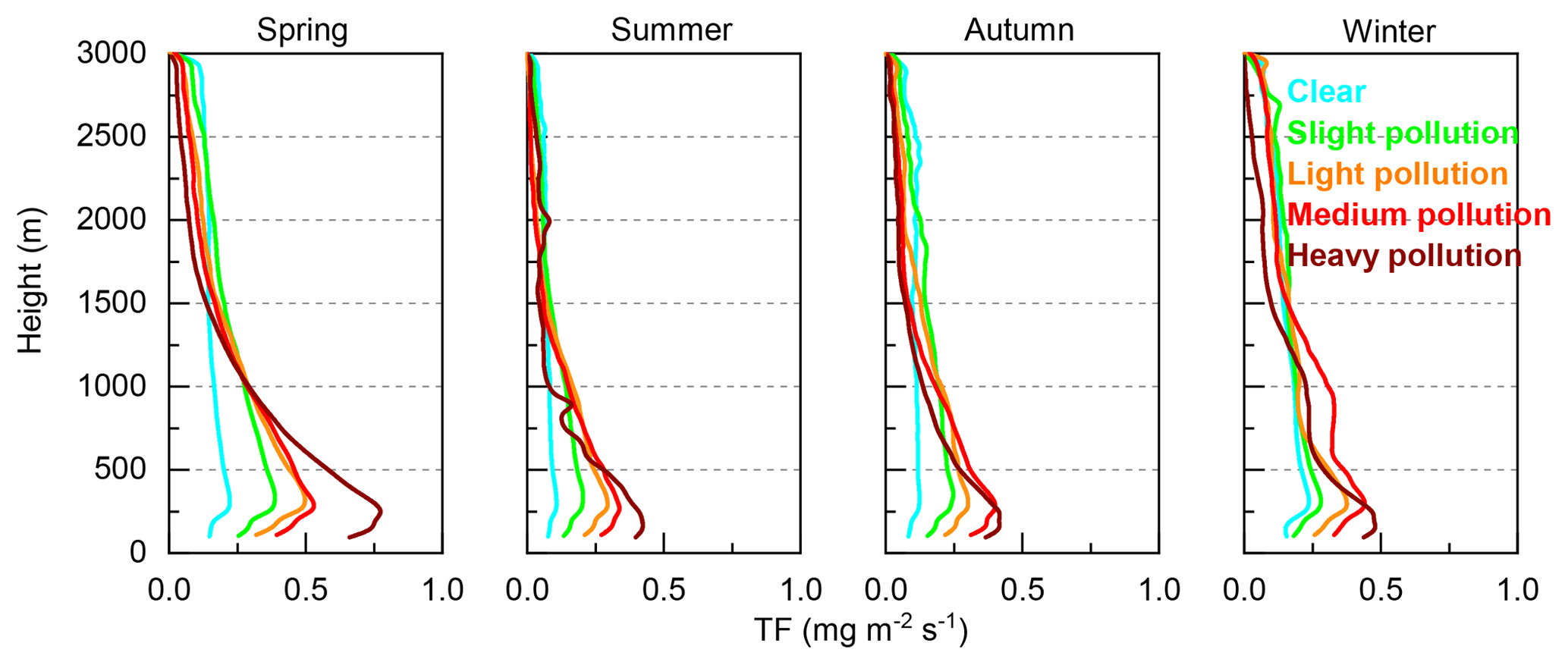
Figure 7 Vertical profiles of TF of PM_2.5 under different degrees of pollution in different seasons in Beijing. Clear days: PM_2.5 ≤ 35 µg m⁻³. Slight pollution: 35 < PM_2.5 ≤ 75 µg m⁻³. Light pollution: 75 < PM_2.5 ≤ 115 µg m⁻³. Medium pollution: 115 < PM_2.5 ≤ 150 µg m⁻³. Heavy pollution: PM_2.5 > 150 µg m⁻³.

3.3 TF under different degrees of air pollution

Previous studies have demonstrated that transport occurs only in the transition period of pollution, while it is weak at the peak of pollution (Tang et al., 2015; Zhu et al., 2016). To quantify the transport impact of different pollution levels, the PM_2.5 concentration was divided into five levels according to the “Technical Regulation on Ambient Air Quality Index (on trial)” (HJ 633-2012): PM_2.5 ≤ 35 µg m⁻³ (clear days), 35 < PM_2.5 ≤ 75 µg m⁻³ (slight pollution), 75 < PM_2.5 ≤ 115 µg m⁻³ (light pollution), 115 < PM_2.5 ≤ 150 µg m⁻³ (medium pollution) and PM_2.5 > 150 µg m⁻³ (heavy pollution). An interesting phenomenon is that with the increase in altitude, the heavier the pollution near the ground is, the greater the reduction rate of the PM_2.5 concentration (Fig. 7). As a result, there is a reversal at 1000–1500 m. In other words, the more severe the near-surface pollution, the lower the high-altitude PM_2.5 concentration. This is particularly outstanding in the spring: from a clear to a heavy polluted day, the TF at 100 m was, in turn, 0.15, 0.26, 0.32, 0.39 and 0.66 mg m⁻² s⁻¹, and at 2600 m, the values dropped to 0.15, 0.17, 0.13, 0.10 and 0.07 mg m⁻² s⁻¹, respectively. That is, the lower the pollution degree, the more vertical the TF tends to be. This is related to the MLH because a high MLH is conducive to the diffusion of pollutants in the vertical direction. With the worsening of pollution, the MLH shows a downward trend (Fig. S3).

According to the previous analysis, two peaks may appear in the TF profile, indicating that the transport occurs at two different heights, approximately 200 m (low-altitude transport) and 1000 m (high-altitude transport). Due to the sudden increase in the WS at approximately 200 m, the low-altitude transport at 200 m is the basic transport height, regardless of the season and the degree of pollution. In contrast, the high-altitude transport is quite special and mainly occurs in the winter, when there is significant pollution. A small peak in the TF can also be found on heavy polluted days in the summer. Although the change in the TF profile of medium pollution in the autumn is not as obvious as that in the summer and winter, a small increase can still be seen (Fig. 7). In the case of heavy pollution, the MLH is usually less than 1000 m, while in the case of clear and slight pollution, the MLH is close to the height of high-altitude transport (Fig. S3). Therefore, it can be inferred that the pollutants transported at a high altitude during heavy pollution are stored in the residual layer, and when the mixing layer becomes higher, the pollutants stored in the residual layer diffuse into the mixing layer, affecting the pollution level within the mixing layer. This may be a key contributor to the slight pollution in the summer, autumn and winter, but further research is needed.

According to the same division method, we further explored the seasonal variation in the TF and transport source in the mixing layer under different pollution degrees. With pollution aggravation, the mixing layer TF in Beijing increased by varying degrees during different seasons, and the transport direction gradually shifted from northwest to south (except during the winter; Fig. 8). In particular, the mixing layer TF in the spring is significantly higher than that in the other seasons at all pollution degrees, which is 1.1–2.0 times that in the other seasons. This may be caused by the greater amount of dust during the spring. With the pollution deterioration, the TF showed an increasing trend in the initial stage of pollution and a decreasing trend during the heavy pollution period. From medium pollution to heavy pollution, the TF decreased from 5.50±4.83 to 4.69±4.84 mg m⁻¹ s⁻¹in the spring, from 3.94±2.36 to 3.39±1.77 mg m⁻¹ s⁻¹ in the summer, from 3.72±2.86 to 3.01±2.40 mg m⁻¹ s⁻¹ in the autumn and from 4.45±4.40 to 3.25±2.77 mg m⁻¹ s⁻¹ in the winter. Among them, the largest drop was found in the winter. In the winter, with the pollution aggravation, the transport direction changed from northwest to southwest and finally to the north. In contrast to in the other seasons, the weak northern wind was the main wind during heavy pollution in the winter, indicating that regional transport contributed less to the heavy pollution during the winter in Beijing. In the initial stage of pollution, the TF continued to increase, but the rate of increase gradually slowed in the spring and summer. From light pollution to medium pollution, the TF decreased by 0.1 mg m⁻¹ s⁻¹ in the spring and increased by only 0.07 mg m⁻¹ s⁻¹ in the summer. It is also not difficult to find from the changes in the TF profile (Fig. 7) that the regional transport has little impact on the medium pollution in the spring and summer. These results indicate that although the region south of Beijing is the main transport source in Beijing, its contribution is significantly reduced during the severe pollution period. In general, regional transport plays an important role in the initial period of pollution, while local emissions are the main controlling factor during the period of heavy pollution. The parabolic pattern of the TF is the result of a combination of the WS and PM_2.5 concentration. The TF reaches a threshold during medium pollution, which is the critical moment mentioned above.

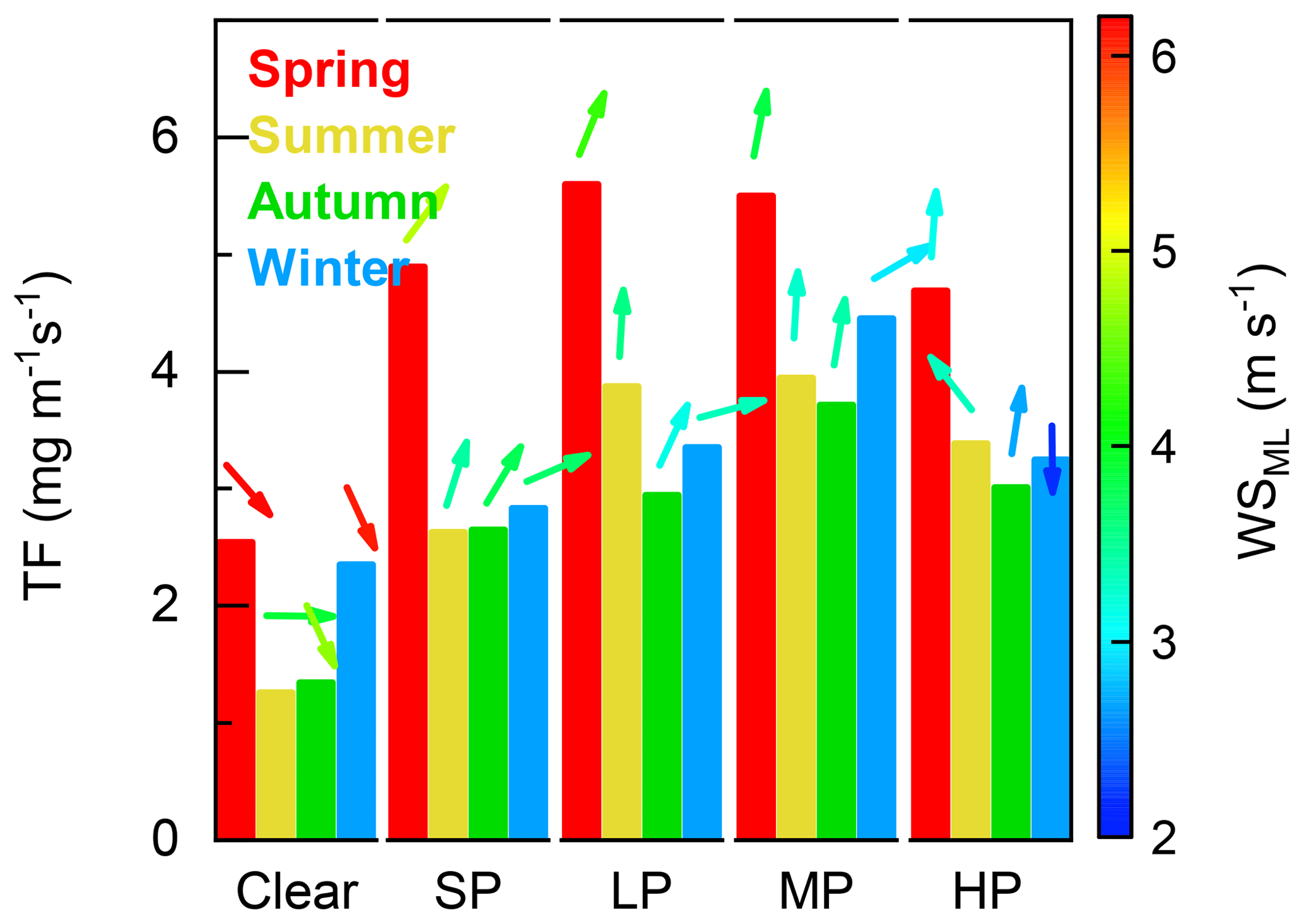
Figure 8 The mixing layer TF of the PM_2.5 levels and transport directions under different degrees of pollution in different seasons in Beijing. (SP denotes slight pollution, LP denotes light pollution, MP denotes medium pollution and HP denotes heavy pollution.)

4 Conclusions

To understand the characteristics of the PM_2.5 transport flux in Beijing, the height of the atmospheric mixing layer and the wind profile within the mixing layer in Beijing were observed for a 2-year period. The main conclusions are as follows:

1. By analyzing the variations in the VC, it is found that the atmospheric dilution capability in Beijing is strongest in the spring and weaker in the summer, autumn and winter. In the spring, the vertical and horizontal dilution capacities are strong, in the autumn and winter, the vertical and horizontal dilution capacities are weak, and in the summer, the vertical dilution capability is strong and the horizontal dilution capability is weak. The diurnal variation in the VC is consistent with the MLH, which shows that the dilution capability is the strongest before sunset, gradually weakens after sunset and remains stable at night. In the spring, the vertical and horizontal dilutions are strong during both day and night. In the winter, the vertical dilution is weak during the day, and the horizontal dilution during the night is the main component. In the summer, the vertical dilution during the day is dominant. Although there is little difference in the diffusivity between the summer, autumn and winter, the poor dilution capability occurs more frequently in the autumn and winter.

2. The TF is the largest in the spring and smaller in the summer, autumn and winter in Beijing. The high TF mainly comes from southward transport, while the low TF is accompanied by northwestern transport. The transport mainly occurred between 14:00 and 18:00 LT, and the height of the transport is at approximately 200 and 1000 m. Using the PM_2.5 concentration as a classification index for the air pollution, the results show that the regional transport from the southern area plays an important role in the initial period of pollution, and local emissions are the main controlling factors in the heavy pollution period, especially in the winter.

To solve the problem of heavy pollution in northern China, joint prevention and control has been suggested for a long time. Even so, there is still no concrete implementation plan. To break through this embarrassing situation, this study quantifies TF to explain the time period when the transport occurs and to identify the main areas affected in Beijing. In this study, the atmospheric dilution capability during different seasons and the TF during different pollution periods were also discussed. The important role of transport in the initial period of pollution is emphasized, and local pollutant emission control is found to be the most effective way of mitigating pollution levels. The research results are of great significance to the early warning, prevention and control of atmospheric particulate pollution.