On the representation of major stratospheric warmings in reanalyses

Major sudden stratospheric warmings (SSWs) represent one of the most abrupt phenomena of the boreal wintertime stratospheric variability, and constitute the clearest example of coupling between the stratosphere and the troposphere. A good representation of SSWs in climate models is required to reduce their biases and uncertainties in future projections of stratospheric variability. The ability of models to reproduce these phenomena is usually assessed with just one reanalysis. However, the number of reanalyses has increased in the last decade and their own biases may affect the model evaluation.

Here we compare the representation of the main aspects of SSWs across reanalyses. The examination of their main characteristics in the pre- and post-satellite periods reveals that reanalyses behave very similarly in both periods. However, discrepancies are larger in the pre-satellite period compared to afterwards, particularly for the NCEP-NCAR reanalysis. All datasets reproduce similarly the specific features of wavenumber-1 and wavenumber-2 SSWs. A good agreement among reanalyses is also found for triggering mechanisms, tropospheric precursors, and surface response. In particular, differences in blocking precursor activity of SSWs across reanalyses are much smaller than between blocking definitions.

1 Introduction

Major sudden stratospheric warmings (SSWs) constitute the most important phenomena of the Northern Hemisphere polar stratospheric variability in wintertime. They are abrupt warmings of the polar stratosphere that lead to a deceleration of the polar vortex and a reversal of the typical westerly circulation (Andrews et al., 1987). SSWs can be classified into two different types according to the structure of the polar vortex during the event. Accordingly, the polar vortex is either displaced from the polar cap (vortex displacement, D SSWs) or split into two parts of similar size (vortex split, S SSWs) (Charlton and Polvani, 2007).

SSWs represent a clear example of stratosphere–troposphere coupling in both directions. First, they are usually preceded by an enhancement of wave activity (e.g., Matsuno, 1971). Although this enhancement can take place in the lower troposphere, recent studies have shown that it often happens within the stratosphere or tropopause region and depends on the stratospheric mean flow conditions (Sjoberg and Birner, 2014; Birner and Albers, 2017; de la Cámara et al., 2017; White et al., 2019). The sources of upward-propagating wave activity are mainly located in the mid-to-upper troposphere and correspond to anomalous circulation events such as a deepened Aleutian low (e.g., Garfinkel et al., 2010) or blocking highs, among others (e.g., Martius et al., 2009; Nishii et al., 2011; Ayarzagüena et al., 2011; Barriopedro and Calvo, 2014). Based on the wave activity preceding SSWs, they are commonly classified into wavenumber-1 (WN1) or wavenumber-2 (WN2) events (e.g., Bancalà et al., 2012; Barriopedro and Calvo, 2014). This classification produces subsets of events similar to the D∕S catalogue. However, there are differences since the former is based on the precursory wave activity while the D∕S classification accounts for the shape of the polar vortex during the post-warming phase (Bancalà et al., 2012). Depending on the type of SSWs, the tropospheric precursors are different and/or located in different geographical locations (Martius et al., 2009; Cohen and Jones, 2011; Bancalà et al., 2012). In particular, differences in blocking precursors are larger when SSWs are classified into WN1/WN2 rather than D∕S (Barriopedro and Calvo, 2014).

In terms of downward coupling, the SSW signal propagates downward and reaches the troposphere as revealed from composite analyses (Baldwin and Dunkerton, 2001), although there is still uncertainty about this tropospheric response when analyzing individual events (e.g., Gerber et al., 2009). One of the suggested factors that may contribute to the spread of the surface signature of SSWs is the type of event. However, while some studies have shown that only S SSWs have large effects on surface climate (Mitchell et al., 2012; Seviour et al., 2013), others have not found consistent differences between S and D SSWs in its significant surface impact (Charlton and Polvani, 2007; Cohen and Jones, 2011). Thus, there is not yet a consensus in this regard, probably due to the differences in the algorithms used to identify S and D SSWs (Maycock and Hitchcock, 2015). As for WN1 and WN2 SSWs, their surface signature has not yet been explored.

SSWs are a key element when analyzing stratospheric variability. The frequency and seasonality of SSWs are common metrics to assess the effects of tropospheric and oceanic phenomena on the polar night jet (PNJ). These metrics are also used to evaluate the stratospheric response to climate change (e.g., Taguchi and Hartmann, 2006; Charlton-Perez et al., 2008; Ayarzagüena et al., 2018). Indeed, in modeling studies most of them use simulations that are previously validated by comparing their results with reanalysis datasets (e.g., Charlton et al., 2007; McLandress and Shepherd, 2009; Kim et al., 2017). However, the number of reanalyses has increased in the last decade; although the observational data used in the assimilation process are the same, the reanalysis models are different and so the final products may also be different (Fujiwara et al., 2017). As happens with other atmospheric models, reanalyses also have biases and this can affect the model evaluation (Fujiwara et al., 2017).

Due to quality improvements associated with the assimilation of satellite data, modern reanalyses, such as ERA-Interim, NASA-MERRA, and NCEP-CFSR, only cover the post-satellite period since 1979. This means that the number of available reanalyses to assess the model performance in the pre-satellite era is smaller than in the post-satellite period. In addition, the amount of data to assimilate is also limited in the former period. All this might produce artificial differences in results before and after the inclusion of satellite data. Gómez-Escolar et al. (2012) documented a change in some SSW features from the pre-satellite to the post-satellite era in NCEP-NCAR and ERA-40 reanalyses. For instance, the intraseasonal distribution and the amplitude of the SSW-associated warming showed differences between both periods, potentially due to a change in the type of assimilated data. With the availability of the new JRA-55 reanalysis, which is the only one that applies an advanced data assimilation scheme to upper-air data during the pre-satellite era, revisiting this topic seems appropriate.

In this study, we aim to assess the performance of the most widely used reanalyses in representing SSWs. To do so, first the main characteristics of SSWs are examined for all datasets to quantify the degree of agreement across reanalyses. Both pre- and post-satellite periods are compared to investigate whether discrepancies among reanalyses in the representation of the main SSW characteristics depend on the examined period. Secondly, we address the dynamical forcing of SSWs in all datasets, including precursors such as blockings. Finally, the surface impact of SSWs retrieved from the different reanalyses is analyzed. Special emphasis is given to the assessment and robustness of the potential differences in the forcing and surface impact of WN1 and WN2 SSWs, as well as S and D events.

Our work is a contribution to Chapter 6 of the Stratosphere-troposphere Processes And their Role in Climate (SPARC) Reanalysis Intercomparison Project (S-RIP) initiative, which aims to assess stratosphere–troposphere coupling in reanalyses. In the framework of this initiative, a few recent studies have addressed some aspects of the representation of polar stratospheric variability in reanalyses. In particular, Martineau et al. (2018) and Hitchcock (2019) also investigate SSW-related aspects. The former analyzes the momentum budget during SSWs restricted to the post-satellite period, while Hitchcock (2019) compares the representation of stratosphere–troposphere coupling in both pre and post-satellite periods, with an emphasis on the impact of including pre-1979 data. Different from these studies, our work provides a comprehensive inter-reanalyses comparison of the most important and typical aspects and processes associated with SSWs in both pre- and post-satellite eras. Additionally, we explore further the characteristics of WN1 and WN2 SSWs that have not yet been investigated.

The structure of the paper is as follows. The data used and methodology applied are described in Sect. 2. Section 3 compares the performance of the main characteristics of SSWs across reanalyses. Section 4 focuses on the dynamical forcing of the events and Sect. 5 addresses the performance of reanalyses in representing the surface impact of SSWs. The main conclusions are summarized in Sect. 6.

2 Data and methodology

2.1 Data

We have used daily data from the following reanalyses: ERA-40 (Uppala et al., 2005), ERA-Interim (Dee et al., 2011), JRA-25 (Onogi et al., 2007), JRA-55 (Kobayashi et al., 2015), NASA-MERRA (Rienecker et al., 2011), NCEP-CFSR (Saha et al., 2010), NCEP-DOE (Kanamitsu et al., 2002), and NCEP-NCAR reanalysis (Kalnay et al., 1996). More details about the different reanalyses can be found in Fujiwara et al. (2017). For the comparison across different reanalyses, all data were used at the common regular grid of 2.5^∘ long × 2.5^∘ lat. When not directly available from the reanalysis centers, a first-order conservative remapping was applied.

The methodology for the intercomparison follows the S-RIP specifications. As such, the analysis has been carried out for two different periods: historical (1958–1978) and comparison (1979–2012). Given the periods covered by each reanalysis, only ERA-40, NCEP-NCAR, and JRA-55 are employed in the historical period. In contrast, all the above listed reanalyses are used in the comparison period with the exception of ERA-40, because it ends in 2002. The performance of each reanalysis is evaluated against a multi-reanalysis mean (MRM), herein considered an “unbiased” reference. In the historical period the MRM refers to the average of the three reanalyses that cover that period, while in the comparison period, the MRM is defined as the average of the most recent reanalyses of each center (ERA-Interim, NCEP-CFSR, JRA-55, and NASA-MERRA). Hereafter, anomalies for each reanalysis are defined as the departure of the field from the daily climatology of each reanalysis. In the historical period, the climatology covers the whole period (i.e., 1958–1978), whereas the comparison period uses the 1981–2010 baseline. Unless otherwise stated, statistical significance of the results is computed with a Monte Carlo test of 1000 permutations, each one containing the same number of cases and dates as the SSWs of each composite but with random years of occurrence.

2.2 Criteria for the identification of SSWs

We have used the list of SSWs and common dates identified by Butler et al. (2017) and provided for the S-RIP initiative (Chapter 6), unless otherwise indicated. First, for each reanalysis, SSWs are identified based on the reversal of the zonal-mean zonal wind at 60^∘ N and 10 hPa between November and March, with at least 20 d of separation between events. Stratospheric final warmings are excluded by requiring at least 10 consecutive days of westerly winds before the end of April (Charlton and Polvani, 2007). The first day of reversal of winds determines the date of occurrence of the SSW (the so-called central date). Common SSWs are those identified by at least two of the three reanalyses in the historical period and by at least four out of seven reanalyses in the comparison period around the same date (usually within 1 or 2 d). The central date of these common events is computed as the median of the central dates from the SSWs detected for each reanalysis. Thus, with this approach, the same events and central dates apply for all reanalyses even if the reversal of the winds does not occur in all of them. This is useful to ensure that the differences between datasets are not due to the selection of different events or dates. The common SSWs are listed in Table 1 for the comparison period.

Table 1 Classification of the common SSWs into WN1 and WN2 events in the comparison period. (In brackets the S∕D classification.)

Nevertheless, in the very first part of our study, we have addressed the opposite question and quantified the possible discrepancies in the frequency of SSWs among reanalyses when the same criterion is applied to all datasets. In that case, we have imposed the World Meteorological Organization definition for the identification of SSWs in each reanalysis. The definition is based on the reversal, within ±5 d, of zonal-mean zonal wind at 10 hPa and 60^∘ N and zonal-mean temperature difference between 90 and 60^∘ N at the same level (Labitzke, 1981).

2.3 Types of SSWs

SSWs are classified following two definitions: D vs. S SSWs and WN1 vs. WN2 events. In this study, D and S SSWs were identified according to the algorithm by Kiyotaka Shibata, which is similar to that by Charlton and Polvani (2007). It is based on the identification of cyclonic vortices and their relative sizes by means of the non-zonal absolute vorticity at 10 hPa from 5 d before to 10 d after (i.e., [−5, 10] d) with respect to the occurrence of an SSW, according to the definition of Sect. 2.2. More specifically, S SSWs are identified when two local maxima of the absolute vorticity are located diametrically opposed and the size ratio of the sectors around those maxima is larger than 0.5 during at least 1 d of the 16 d period surrounding the SSW. Otherwise the SSW is defined as D. The events were classified individually in each reanalysis. The classification into S∕D events of common SSWs in the comparison period (used in Sects. 4 and 5) was based on the predominant type of each single event across the different reanalyses, following a similar procedure to that employed for the identification of the common dates (Table 1).

WN1 and WN2 SSWs were selected by applying a zonal Fourier decomposition of the daily 50 hPa geopotential height data at 60^∘ N into WN1 (Z₁) and WN2 (Z₂) amplitudes for the [−10, 0] d period before each SSW (Barriopedro and Calvo, 2014). An SSW was defined as a WN2 event if [Z₂] ≥ [Z₁] (brackets denote the averaged amplitude for the [−10, 0] d period before the SSW) or if $Z_{\mathrm{2}}-Z_{\mathrm{1}}\ge \mathrm{200}$ m at least for 1 d within the [−10, 0] d period before the SSW. Otherwise, the SSW was defined as a WN1 event. See the list of events of each type in Table 1 and Barriopedro and Calvo (2014) for more details on the algorithm.

2.4 Dynamical benchmarks

We have applied the following diagnostics proposed by Charlton and Polvani (2007) to evaluate the dynamical signatures associated with the occurrence and development of SSWs:

• Amplitude of the SSW in the middle stratosphere (hereafter amp010) computed as the area-weighted mean 10 hPa temperature anomaly over the polar cap (50–90^∘ N) and averaged for the [−5, 5] d period with respect to the central date of the event.

• Amplitude of the SSW in the lower stratosphere (hereafter amp100), defined as amp010 but at 100 hPa. It provides a measure of the coupling between the middle and lower stratosphere around the occurrence of SSWs.

• Deceleration of the PNJ (hereafter decelu), corresponding to the difference of the 10 hPa zonal-mean zonal wind at 60^∘ N between the [−15, −5] d period prior to the central date and the [0, 5] d period after the central date.

• Wave activity prior to SSW (hereafter actwav), computed as the area-weighted mean 100 hPa meridional eddy heat flux (HF) anomaly averaged over 45–75^∘ N for the [−20, 0] d period before the occurrence of the event.

2.5 Upward-propagating wave activity

The anomalous meridional eddy HF averaged over 45–75^∘ N at different pressure levels was used as a metric to measure the upward propagation of wave activity. This latitudinal band corresponds to the climatological area with the strongest vertical wave propagation from the troposphere to the stratosphere (Hu and Tung, 2003).

As a second step, the methodology by Nishii et al. (2009) was applied to analyze the role of different forcing processes in the occurrence of SSWs. This methodology is based on the decomposition of daily anomalous eddy HF into two components, which correspond to the interaction between climatological waves and anomalous waves (second and third right-hand terms of Eq. 1) and the inherent contribution of anomalous waves (first right-hand term of Eq. 1):

$$\begin{array}{}\text{(1)}& {\left[v^{\ast }{T}^{\ast }\right]}_{\mathrm{a}}={\left[v_{\mathrm{a}}^{\ast }{T}_{\mathrm{a}}^{\ast }\right]}_{\mathrm{a}}+\left[v_{\mathrm{c}}^{\ast }{T}_{\mathrm{a}}^{\ast }\right]+\left[v_{\mathrm{a}}^{\ast }{T}_{\mathrm{c}}^{\ast }\right],\end{array}$$

where brackets and asterisks indicate zonal mean and deviation from it, respectively; v is meridional wind; T is temperature; and the a and c subscripts denote daily anomalies and climatological values, respectively. Equation (1) has been applied to each pressure level.

2.6 Blocking definitions

The precursor role of blocking in SSWs has been discussed across studies (e.g., see Castanheira and Barriopedro, 2010, for an overview), although there is not a clear consensus on this topic. The divergent results of previous studies may partially be attributed to different methodologies of blocking detection (e.g., Woollings et al., 2008). In this study, three different blocking definitions have been used to address this question. The three methodologies use daily geopotential height at 500 hPa (Z500) and span almost all approaches to blocking definition. The first method is based on the occurrence of regional and persistent meridional Z500 gradient reversals (the absolute method, ABS; e.g., Scherrer et al., 2006). The second metric involves the detection of persistent and quasi-stationary Z500 anomalies, computed with respect to the local climatological field (the anomaly method, ANO; e.g., Sausen et al., 1995). Finally, a combined method of absolute and anomaly Z500 fields (the mixed method, MIX) is used, providing a double perspective of blocking (Barriopedro et al., 2010). Several criteria are imposed to ensure that the detected episodes represent large-scale, quasi-stationary, and persistent high-pressure systems. See Woollings et al. (2018) for more details about blocking definitions.

3 Main SSW characteristics

In this section, the main signatures of SSWs (frequency, type of events, and process-based diagnostics) are analyzed for each period and compared among the different datasets.

Table 2 Frequency of SSWs per decade and ratio of vortex displacement (D) vs. vortex split (S) SSWs for each reanalysis and period of study.

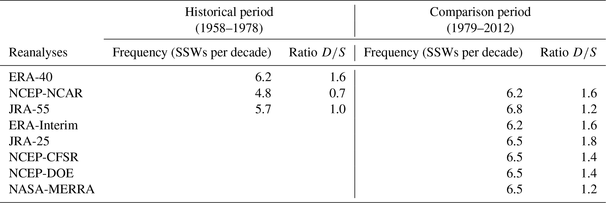
3.1 Frequency, seasonality, and type of events

First, we have analyzed the results for the frequency and type of events when the same criterion is applied to each dataset. Table 2 shows the mean frequency of events and the ratio of D to S SSWs for each period and reanalysis. The main differences are found in the historical period when the reanalyses show a large spread in both frequency and type of events. In particular, the NCEP-NCAR reanalysis displays the results that deviate the most from the other two datasets, although the differences are not statistically significant at the 95 % confidence level (Student's t test). The short period of analysis and hence the reduced sample might explain part of these discrepancies. More importantly the unavailability of satellite data in the pre-satellite era leads to a strong dependency of the reanalysis data in the stratosphere on the characteristics of each reanalysis model. Note that NCEP-NCAR reanalysis is the only reanalysis with a low-top model and a lid in the stratosphere (3 hPa), whereas JRA-55 and ERA-40 have the top in the mesosphere (0.1 hPa). The low top typically dampens variability close to the top and so reduces the probability of the occurrence of an SSW (Charlton-Pérez et al., 2013). In fact, the standard deviation of daily polar temperature and zonal wind at 10 hPa in December and January of the historical period is much lower in NCEP-NCAR than in the other two reanalyses, although the differences are not statistically significant at the 95 % confidence level (Fisher F test) (Fig. 1a, c). In contrast, at lower levels, we do not find such discrepancies (see 100 hPa temperature in Fig. 1b, d), supporting that the occurrence of SSWs during this period is strongly influenced by the model performance and hence should be considered reanalysis dependent.

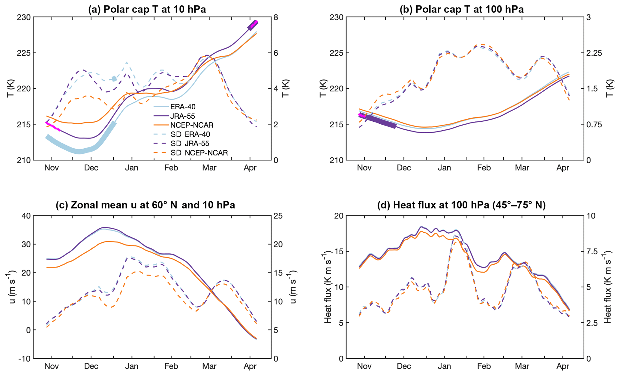
Figure 1 The 21 d running mean of the daily climatology (solid lines) and standard deviation (dashed lines) in the historical period (1958–1978) of (a) polar-cap (50–90^∘ N) averaged temperature at 10 hPa, (b) polar-cap (50–90^∘ N) averaged temperature at 100 hPa, (c) zonal-mean zonal wind at 60^∘ N and 10 hPa, and (d) heat flux at 100 hPa averaged over 45–75^∘ N. The left (right) y axis refers to the mean (standard deviation) in each plot. Thick lines indicate values of ERA-40 or JRA-55 that are significantly different from those of NCEP-NCAR reanalysis at the 95 % confidence level. Magenta crosses correspond to JRA-55 values that are significantly different from ERA-40 ones at the 95 % confidence level (Student's t test).

Conversely, in the comparison period, there is a good agreement in both the frequency and ratio of D∕S SSWs. Small differences are found, particularly in the D∕S ratio, but this might be due to the specific thresholds or other methodological issues of the applied criterion since such deviation does not appear when classifying SSWs into WN1 and WN2 events (Barriopedro and Calvo, 2014). More details about these classifications of SSWs can be found in Chapter 6 of S-RIP.

Regarding SSW seasonality, Fig. 2 shows the smoothed seasonal distribution of SSW per decade. This distribution has been computed by counting the number of SSWs within the ±10 d periods centered on each winter day. Additionally, the distribution has been smoothed with a 10 d running mean. Similar to the winter mean frequency of SSWs, historical reanalyses show the largest spread in the seasonal distribution. A substantial part of this spread is due to the NCEP-NCAR reanalysis whose distribution is statistically significantly different from that of the other two reanalyses at a 99 % confidence level (two-sample Kolmogorov–Smirnov test). In contrast, ERA-40 and JRA-55 distributions display similar (statistically undistinguishable) distributions. In particular, they show an increasing SSW occurrence from early winter that maximizes in January and decreases by late winter (Fig. 2a), in agreement with the temporal evolution of the standard deviation of the zonal-mean zonal wind at 60^∘ N and 10 hPa in the historical period (Fig. 1c). In contrast, SSWs for NCEP-NCAR are more uniformly distributed with three sharp maxima in early, mid, and late winter. The early winter peak of SSWs in NCEP-NCAR agrees well with the climatological polar stratospheric state, which shows a weaker PNJ and a warmer polar stratosphere than the other two reanalyses (Fig. 1a and c). These NCEP-NCAR differences from the other historical reanalyses are only statistically significant for the polar stratospheric temperature and ERA-40, though likely due to the short sample and the generally large interannual variability of the winter polar stratosphere. However, they agree with an artificial positive temperature trend of 8 ^∘C at 10 hPa for 1948–1998 in the NCEP-NCAR reanalysis, as documented by Badin and Domeisen (2014). On the other hand, the lower wind variability in January in NCEP-NCAR would agree with the reduced frequency of SSWs in that month and reanalysis, as compared to the other datasets. In the comparison period the results are similar across reanalyses, which show statistically indistinguishable distributions (two-sample Kolmogorov–Smirnov test, Fig. 2b). In this period, the maximum occurrence shifts to late winter in all datasets compared to the distributions of ERA-40 and JRA-55 in the historical period. Similar differences in the intraseasonal distribution of events were already documented by Gómez-Escolar et al. (2012) between the pre- and post-1979 periods. Despite the large uncertainty in the earlier period, their distributions are statistically significantly different at the 99 % confidence level and this result supports the hypothesis of multidecadal variations in the intraseasonal occurrence of SSWs, which adds to the reported variability in the total winter frequency of SSWs (Schimanke et al., 2011; Reichler et al., 2012; Domeisen, 2019).

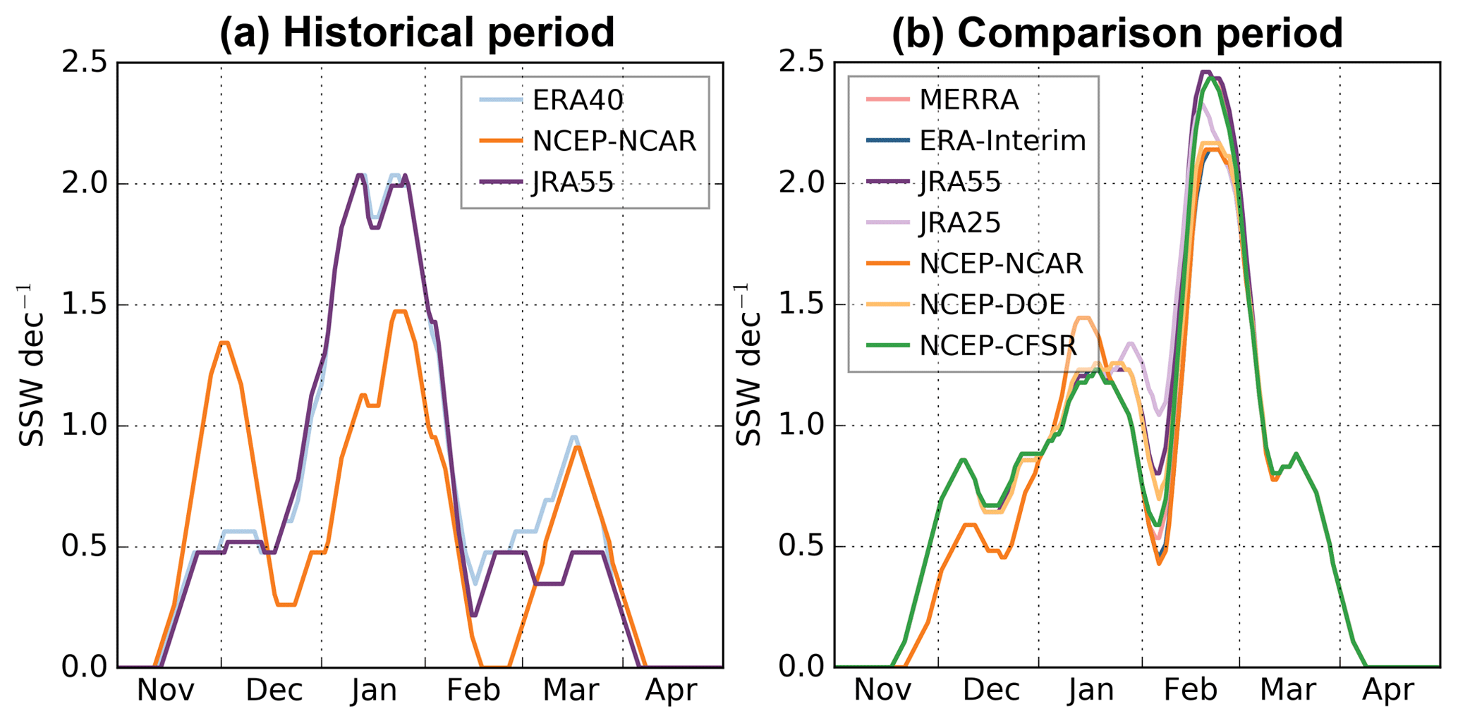
Figure 2 SSW total frequency distribution within ±10 d periods from the date displayed in the x axis for (a) the historical period (1958–1978) and (b) the comparison period (1979–2012). Time series are smoothed with a 10-day running mean.

3.2 Process-based diagnostics

The processes involved in the occurrence of SSWs have been compared across reanalyses by using the diagnostics defined in Sect. 2.4. In this case, and in the rest of the paper, we have used the common dates of SSWs to make sure the differences found across reanalyses are not due to the inclusion of different events.

Figure 3 shows the statistics (mean, median, and interquartile range) of the dynamical benchmarks for all reanalyses in the two periods. A quick comparison of the MRM of these benchmarks for both periods reveals that SSWs are preceded by a similar anomalous strengthening of wave activity at 100 hPa, are associated with a comparable deceleration of the PNJ, and have a similar amplitude in the middle and lower stratosphere in both periods. Only slight differences are found in the median of decelu and amp100 (compare Fig. 3b and c with Fig. 3f and g). However, given that the median and mean of these magnitudes for one period are included within the interquartile range of the other, we can conclude that SSW characteristics are similar in both periods of study.

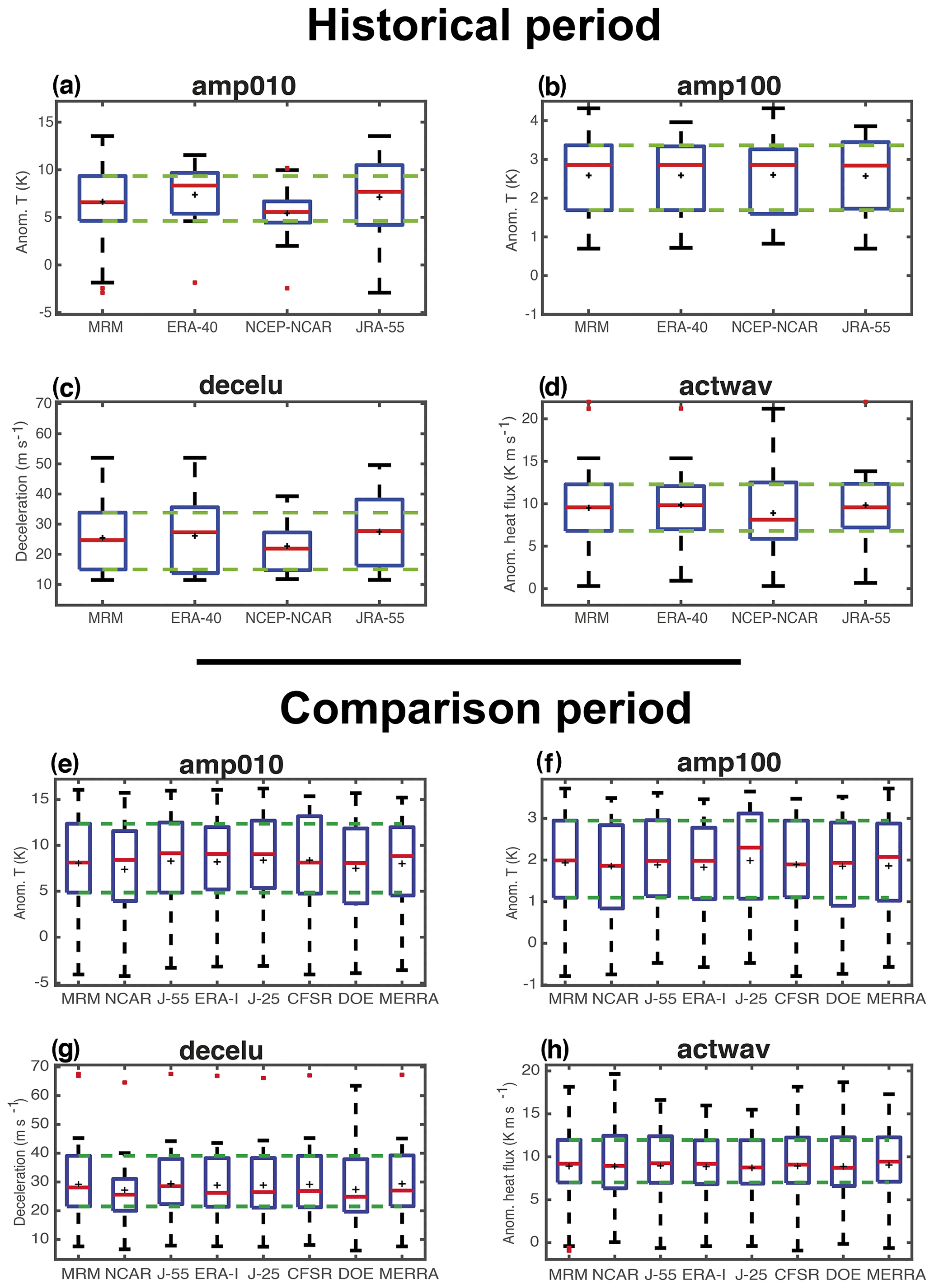
Figure 3 Box plots showing the distribution of the dynamical benchmarks of SSWs (amp010, amp100, decelu, and actwav) in the historical (1958–1978) and comparison (1979–2012) periods. The interquartile range is represented by the size of the box and the red line (black cross) corresponds to the median (mean). Whiskers indicate the maximum and minimum points in the distribution that are not outliers. Outliers (red crosses) are defined as points with values greater than 3∕2 times the interquartile range from the ends of the box. See text for the definition of dynamical benchmarks.

The comparison period shows good agreement among all reanalyses as all datasets are characterized by similar median, mean, and spread values (Fig. 3e–h). Nevertheless, slight deviations can be found for NCEP-NCAR in the distribution of decelu, which is shifted towards lower values and shows a reduced spread among events, as compared to the rest of the datasets (Fig. 3g). These deficiencies are even clearer in the historical period when a similar discrepancy is detected in amp010 (Fig. 3a), consistent with the reduced strength and variability of the PNJ in NCEP-NCAR reanalysis (Fig. 1c). As the deviation of decelu in the NCEP-NCAR reanalysis is common for both periods, this might point to a bias of the model, whose effects are amplified in the first period by the lower amount of assimilated data. As mentioned before, this bias is very likely linked to the low top of the model and the low vertical resolution in the stratosphere, provided that the SSW characteristics at lower levels (i.e., amp100, actwav) do not differ much from those of other reanalyses. Note that these differences are still noticeable in NCEP-DOE, in agreement with Long et al. (2017) that identified similar biases in the climatology and interannual variability of temperature and zonal winds for both NCEP reanalyses. The model of NCEP-DOE is basically the same as that of NCEP-NCAR reanalysis although with an updated version (1995 vs. 1998) (Fujiwara et al., 2017). This implies that both reanalyses use a model with a low resolution in the stratosphere and with assimilated temperature data instead of direct radiances that reduce their ability to represent the stratosphere (Fujiwara et al., 2017). Despite their similarities, the NCEP-DOE performs better with respect to the MRM, particularly for decelu, arguably due to improvements introduced in the updated version of the reanalysis model. Primarily, NCEP-DOE was run with a new ozone climatology (Kanamitsu et al., 2002). Other differences in the concentration of CO₂ or the radiation scheme between both reanalyses might also explain the differences between both NCEP reanalyses (Fujiwara et al., 2017).

A similar analysis has been carried out separately for WN1 and WN2 SSWs in the comparison period (Fig. S1 in the Supplement). All datasets reproduce a similar behavior for both types of events and all diagnostics, with the exception of the associated deceleration of the PNJ in the middle stratosphere: WN2 SSWs are related to larger decelerations of the PNJ, probably because they are usually preceded by a stronger polar vortex than WN1 SSWs (Albers and Birner, 2014; Díaz-Durán et al., 2017). These results also confirm the overall good agreement across reanalyses except for the deficiency of NCEP-NCAR concerning decelu. Unfortunately, these findings cannot be confirmed in the historical reanalyses due to the very low frequency of WN2 events in that period (not shown).

4 Dynamical forcing

4.1 Upward-propagating wave activity

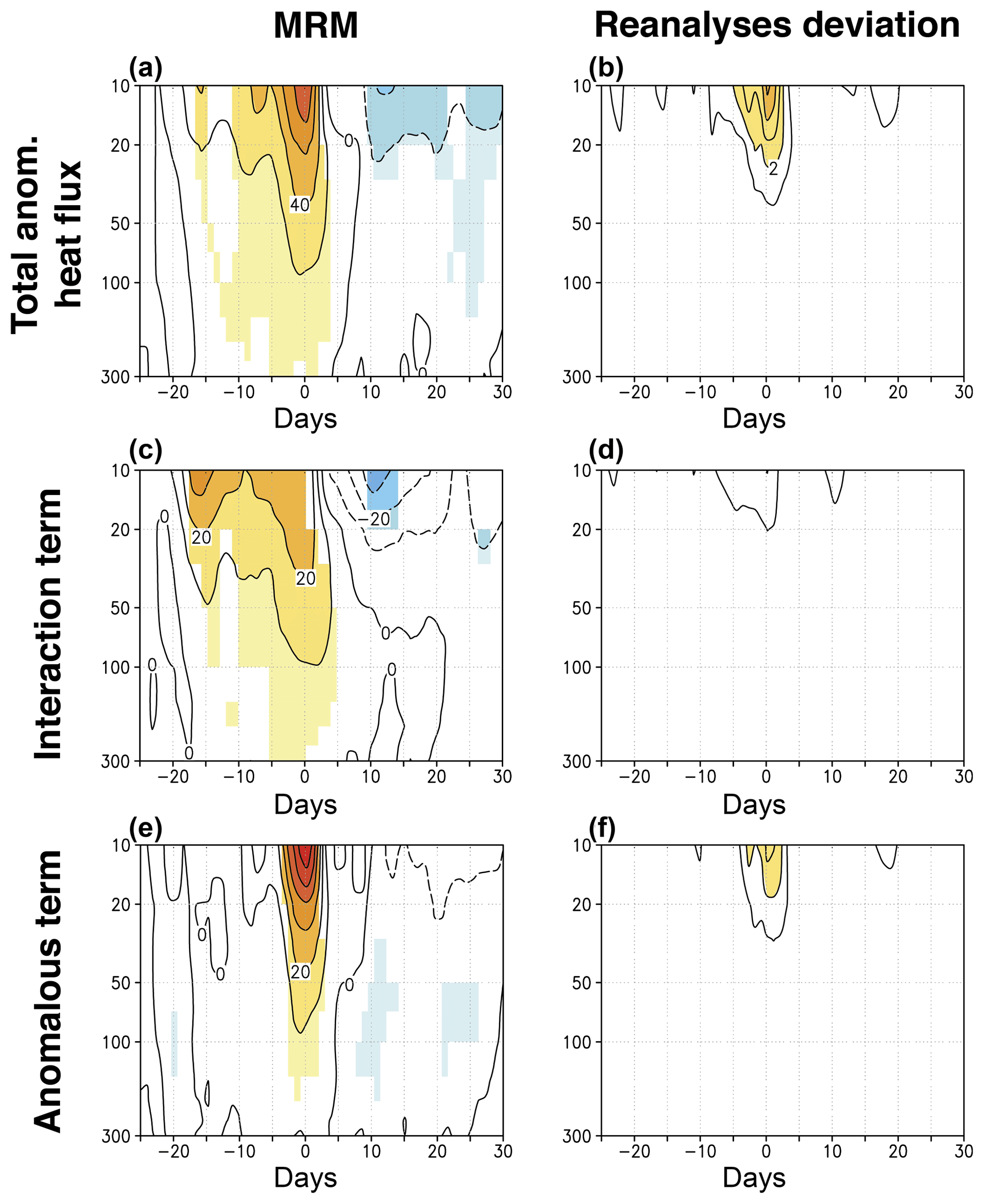
Figures 4 and 5 show the composited anomalous eddy HF, area-averaged between 45 and 75^∘ N, at different levels around the SSW onset date for the historical and comparison periods, respectively. Only results from 300 to 10 hPa are presented, as the [300, 100] hPa layer corresponds to the communication region for the stratosphere–troposphere coupling (de la Cámara et al., 2017) and the levels above this layer typically show the strongest HF anomalies. The MRM shows a strong anomalous peak of HF around the central date of SSWs in both periods. This strong peak is preceded by a weak pulse around [−20, −15] d in the middle stratosphere in the comparison period but not in the historical one. The largest differences across reanalyses are detected in the middle stratosphere in agreement with Martineau et al. (2018), and they are more pronounced for the historical than for the comparison period.

By applying the methodology by Nishii et al. (2009) we have analyzed the contributing role of the different HF terms to the occurrence of SSWs. The MRM decomposition of the HF in the comparison period shows that the strongest peak ([−5,0] d interval) is mainly due to the action of anomalous waves (first right-hand term of Eq. 1), albeit with a relevant contribution of the constructive interaction between climatological and anomalous waves (second and third right-hand terms of Eq. 1) (Figs. 4c and e, and Fig. 5c and e). Conversely, the preceding weaker pulses of the comparison period seem to be more dominated by the interaction term. The agreement among reanalyses concerning the relative roles of these terms is higher for the comparison period, mainly in the middle stratosphere, than for the historical period (compare Fig. 4d and f vs. Fig. 5d and f).

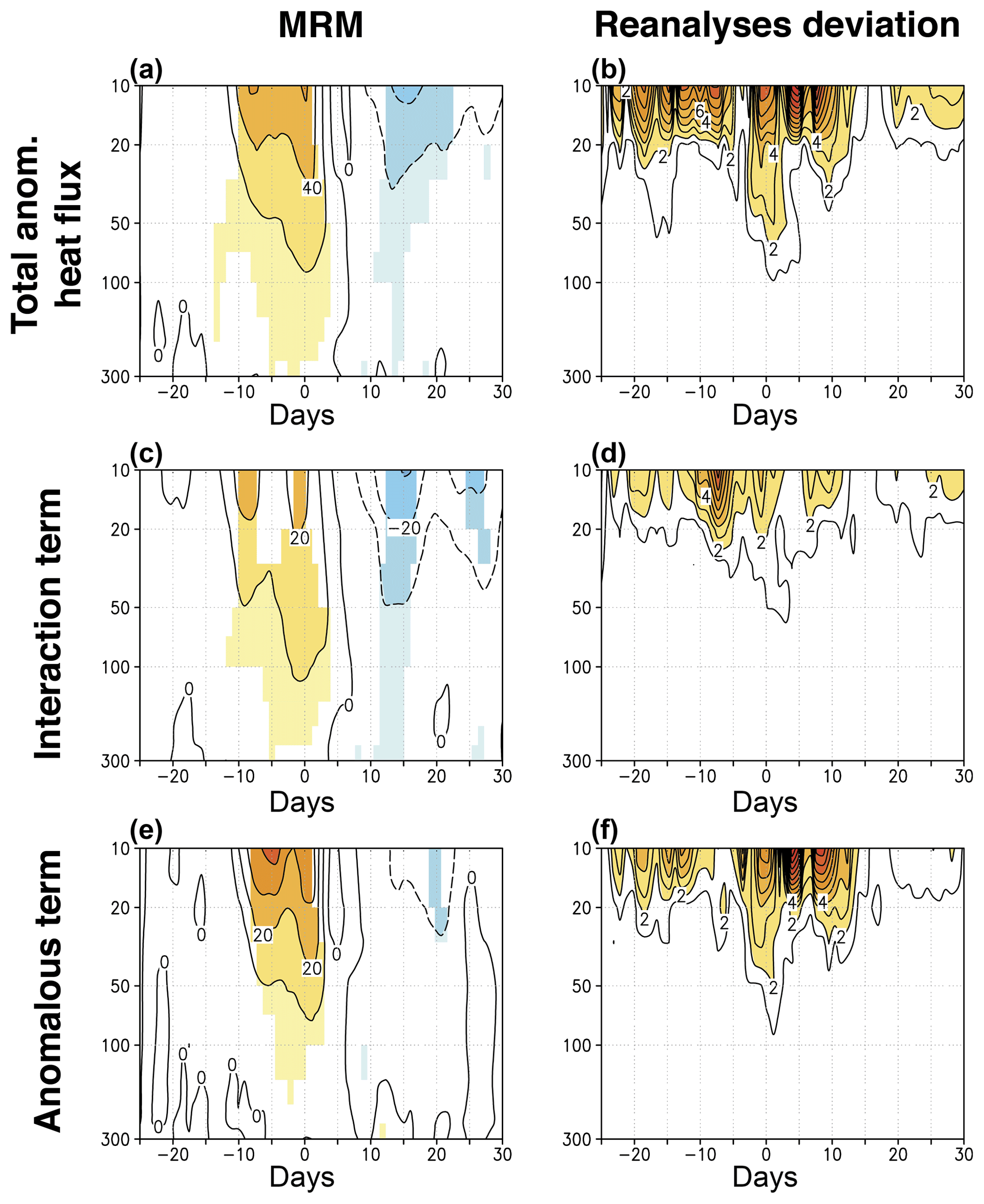
Figure 4 (a) Composited time evolution of the total anomalous heat flux averaged over 45–75^∘ N (K m s⁻¹) at different pressure levels from 29 d before to 30 d after the occurrence of SSWs in the historical period (1958–1978). Contour interval is 20 K m s⁻¹. (b) Same as (a) but for the standard deviation of the reanalyses with respect to the MRM divided by the square root of the number of reanalyses. Contour interval is 1 K m s⁻¹. (c, d) Same as (a) and (b) but for the interaction between climatological and anomalous waves. Contour intervals are 10 and 2 K m s⁻¹, respectively. (e, f) Same as (a) and (b) but for the contribution of the anomalous waves to the total anomalous heat flux. Contour intervals are 10 and 2 K m s⁻¹, respectively. Shading in (a), (c), and (e) denotes statistically significant anomalies at the 95 % confidence level of the same sign in at least 66.7 % of all reanalyses (Monte Carlo test).

Figure 5 Same as Fig. 4 but for the comparison period (1979–2012).

Given the documented differences in the dynamical forcing of different types of SSWs (e.g., Smith and Kushner, 2012; Barriopedro and Calvo, 2014), we have repeated the analysis separately for WN1 and WN2 SSWs (Fig. 6). It has only been done for the comparison period, due to the low sample size of WN2 events for the historical one. Although there is not a univocal relationship between D and S SSWs and WN1 and WN2 events (Waugh, 1997), our results for WN1 and WN2 events agree well with those of Smith and Kushner (2012) for D and S SSWs. WN1 events are mainly triggered by persistent but moderately intense anomalies of HF during different periods ([−20, −15] and [−10, 0] d), which are associated with the constructive interference of climatological and anomalous waves (Fig. 6e and i). In contrast, WN2 events are related to intense but short pulses of eddy HF in the 5 d prior to the central date. These pulses are predominantly due to the anomalous term (Fig. 6g and k), consistent with Smith and Kushner's finding for S SSWs. The recovery of the polar vortex after WN2 SSWs is due to a reduction of wave activity in the interaction term, while only the anomalous term has a statistically significant contribution to this reduction after WN1 SSWs (Fig. 6e, g, i, and k).

Figure 6 Same as Fig. 5 but for (a) WN1 SSWs and (b) WN2 SSWs.

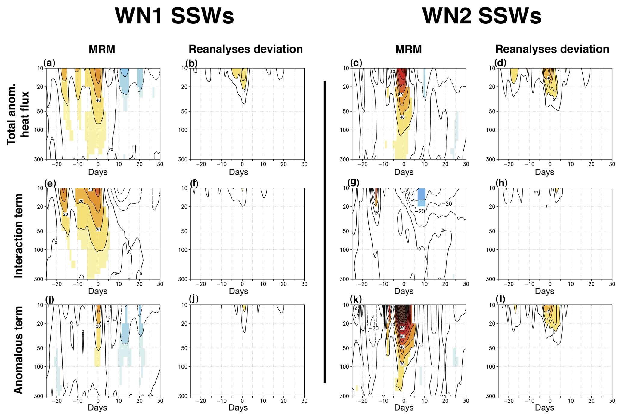
The comparison among reanalyses reveals that all datasets can reproduce the above differences between WN1 and WN2 SSWs. The spread is higher for WN2 SSWs than for WN1 SSWs (Fig. 6b, d, f, h, j, and l), particularly for the anomalous HF term (Fig. 6l). However, considering the differences in HF values between WN1 and WN2 SSWs (i.e., by dividing the standard deviation by the MRM), the resulting spread becomes comparable for both types of SSWs (not shown).

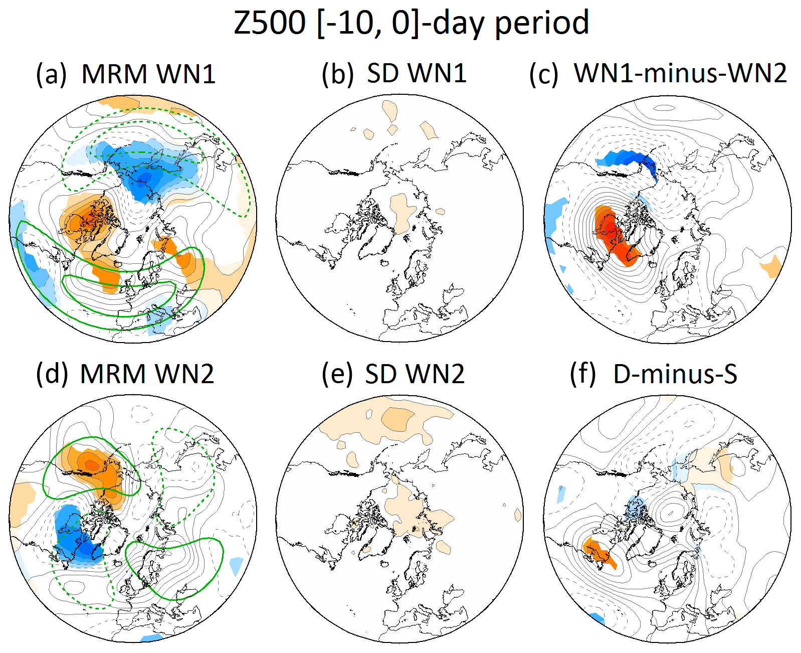
Figure 7 (a) MRM of WN1 SSW-based composites of 500 hPa geopotential height anomalies (contour interval 20 m) in the [−10, 0] d period before events for the comparison period (1979–2012). Only statistically significant anomalies at the 95 % confidence level of the same sign (Monte Carlo test) in at least 66.7 % of all reanalyses are shaded. (b) Standard deviation of the reanalyses with respect to the MRM divided by the square root of the number of reanalyses for WN1 SSWs (contour interval is 1 gpm). (c) Same as (a) but for the WN1 SSW minus WN2 SSW differences in MRM composites of 500 hPa geopotential height anomalies. Shading denotes statistically significant differences at the 95 % confidence level in at least 66.7 % of all reanalyses (Monte Carlo test). (d, e) Same as (a) and (b) but for WN2 SSWs, respectively. (f) Same as (c) but for displacement (D) minus split (S) events. Green contours in (a) and (d) show the MRM climatological WN1 and WN2 of 500 hPa geopotential height from November to March, respectively (contours: ±40 and ±80 gpm).

4.2 Tropospheric circulation anomalies associated with SSWs

To investigate the tropospheric patterns preceding SSWs, we have analyzed the averaged Z500 anomalies in the 10 d prior to the central date of each type of SSW (Fig. 7). As in the previous section, we have focused on the differences between WN1 and WN2 events in the comparison period only. The chosen time window corresponds to the peak of the strongest anomalies of HF in Fig. 5a. It is also the approximate time that planetary waves take to propagate from the troposphere to the stratosphere (Limpasuvan et al., 2004). The results reveal statistically significant differences between the precursors of WN1 and WN2 SSWs (Fig. 7c). The precursor signal for WN1 SSWs shows a predominant WN1-like structure, with negative anomalies of Z500 over the North Pacific and eastern Asia and positive anomalies over northern Canada, the North Atlantic, and western Siberia (Fig. 7a). This agrees with the pattern identified by previous studies such as Limpasuvan et al. (2004) and Garfinkel et al. (2012) for all SSWs. Most of these centers of action project onto the climatological WN1 of the MRM, especially the one over the North Pacific (e.g., Garfinkel and Hartmann, 2008), explaining the high positive values of the interaction term of HF (e.g., Martius et al., 2009; Nishii et al., 2011). Differently, the precursor signal of WN2 SSWs shows strong negative Z500 anomalies over Canada and Greenland and positive anomalies over the northeastern Pacific (Fig. 7d). The main anomalous centers coincide geographically and in sign with the antinodes of the climatological WN2 of the MRM (e.g., Garfinkel and Hartmann, 2008). Although this pattern agrees with the preferred blocking precursors of WN2 SSWs (Barriopedro and Calvo, 2014), it seems counterintuitive with the predominant role of the anomalous waves found in Fig. 6 for these events, although we are looking at very different levels in the two figures. The same apparent contradiction was already highlighted by Smith and Kushner (2012). Nevertheless, the tropospheric and stratospheric results might not be so contradictory as suggested at the first sight. As indicated in the Introduction section, recent studies have given evidence of the importance of the stratospheric contribution in the amplification of anomalous wave activity prior to an SSW (e.g., Sjoberg and Birner, 2014; Birner and Albers, 2017; de la Cámara et al., 2017). This contribution seems particularly relevant in the case of WN2 SSWs, when an initial vortex structure close to its resonant point can split the vortex with only a small increase in tropospheric wave forcing (Plumb, 1981; Albers and Birner, 2014). Based on our results, this tropospheric wave forcing might result from the constructive interference of anomalous and climatological waves.

The agreement among reanalyses is very good (Fig. 7b and e). Only very small differences appear in the tropospheric pattern over the North Pacific, which are larger for WN2 than for WN1 SSWs, in agreement with the comparison of wave activity (Fig. 6). We stress that the largest differences in wave activity among reanalyses are found in the middle stratosphere and hence the Z500 deviations from the MRM are smaller than those in the HF composites. The lower spread among reanalyses in tropospheric fields compared to that in the stratosphere is expected based on the larger number of assimilated data.

4.3 Blocking

The positive Z500 anomalies identified in the previous section may imply an increased blocking frequency over those locations prior to the occurrence of each type of SSW. Similarly, a below-normal activity of blocking before SSWs might translate into negative Z500 anomalies. Here, we identify blocking precursors of WN1 and WN2 SSWs by performing 2-D composites of the blocking frequency (in % of winter days) for the [−10, 0] d period before the central day of SSWs (same window as in Fig. 7). We have employed the three different algorithms described in Sect. 2.6. Figure 8a–c and d–f show the MRM of blocking precursor frequencies for WN1 and WN2 SSWs in the comparison period, respectively. Figure 8g–i displays the MRM of a pseudo-climatology of the blocking frequency prior to all SSWs (see the figure caption for details on its computation). In general, in all methods there is a spatial preference for specific blocking precursors depending on the main wave activity preceding SSWs. For WN1 SSWs, enhanced (above climatology) blocking frequencies are detected over the western Atlantic and east of Scandinavia, and reduced (below climatology) blocking activity occurs over the eastern Pacific (compare Fig. 8a–c vs. Fig. 8g–i). Nearly opposite patterns are identified for WN2 SSWs (compare Fig. 8d–f vs. Fig. 8g–i) except for an increased blocking frequency over east of Scandinavia. These results also agree well with the Z500 pattern preceding each type of SSW in Fig. 7. They are also consistent with previous studies that identified the preferred location of blockings for the intensification of WN1 and WN2 wave activity (e.g., Castanheira and Barriopedro, 2010; Nishii et al., 2011; Barriopedro and Calvo, 2014; Ayarzagüena et al., 2015).

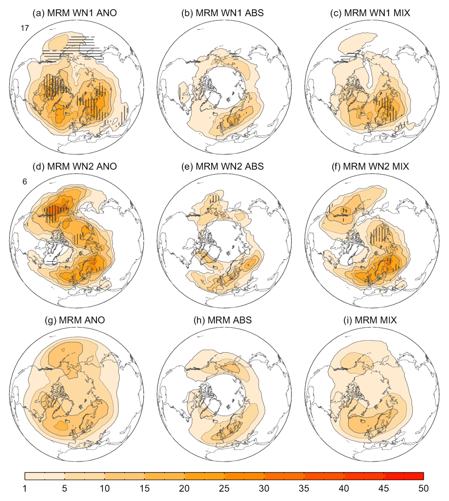
Figure 8 (a–c) MRM of blocking frequency (% of winter days) for the [−10, 0] d period before the central date of WN1 SSWs of the comparison period (1979–2012) for the (a) anomaly (ANO), (b) absolute (ABS), and (c) mixed (MIX) methods. The blocking frequency is expressed as the percentage of time (over the 11 d period) during which a blocking was detected at each grid point. Vertical (horizontal) hatching denotes regions where at least 66.7 % of the reanalyses show a significant increase (decrease) of the frequency with respect to the climatology at the 90 % confidence level. (d–f) Same as (a)–(c) but for WN2 SSWs. (g–i) MRM of the mean blocking frequency in 1000 Monte Carlo trials of 11 d intervals preceding all SSWs dates of the comparison period. In each trial, a set of 11 d intervals prior to the SSWs dates of random years is averaged so that we obtain a pseudo-climatology of the blocking frequency in the same winter moments as when the SSWs took place. This method avoids any effects of the seasonal cycle of the blocking activity during the extended winter (NDJFM) that would affect the result if we averaged directly the blocking activity during that season.

This blocking signal is reproduced by all methods and reanalyses (not shown), although the intensity, significance, and spatial extension of the anomalies vary with the blocking definition. For example, the precursory signal of SSWs in ABS is confined to smaller regions than in ANO and MIX, eventually becoming nonsignificant. These differences between methods do not only refer to the blocking signal prior to SSWs but also to the climatology (Fig. 8g–i), which can be explained by the different aspects captured by each blocking indicator (Barriopedro et al., 2010). Reanalyses show a reasonable agreement in the blocking frequency results and they even agree on the statistical significance of changes in the blocking frequency for the ANO and MIX methods, which show a noticeable deviation from the climatology prior to SSWs. Thus, the disagreement between previous studies regarding the precursor role of blocking in SSWs is better explained by the blocking definition than the chosen reanalysis.

5 Surface signal of SSWs

Finally, the surface signal after the occurrence of SSWs was explored by compositing the mean sea-level pressure (MSLP) anomalies of the [5, 35] d period for all events. The time interval was selected following Palmeiro et al. (2015), who identified the strongest negative values of the Northern Annular Mode (NAM) index in this period. We found a general good agreement in the surface signal of all SSWs across reanalyses in both historical and comparison periods (not shown). Similar to the previous sections, we present here only the MSLP composites for WN1 and WN2 SSWs and the comparison period (Fig. 9a and d). WN1 and WN2 SSWs show a significant negative NAM-like pattern response with positive anomalies over the polar cap in both cases. However, some slight differences between WN1 and WN2 events are found. Over the northeastern Pacific, MSLP anomalies of different sign (positive for WN2 SSWs and negative for WN1 SSWs) were also detected prior to the occurrence of SSWs (see Fig. 7 and also in MSLP maps, not shown). Thus, they may be a remainder of the tropospheric precursors, as also suggested by Charlton and Polvani (2007). In the European Atlantic sector, negative anomalies after WN1 SSWs extend over the whole Atlantic Ocean and western and central Europe (Fig. 9a), while those related to WN2 SSWs are shifted towards Eurasia (Fig. 9d). Nevertheless, these differences are only statistically significant in western and central Europe and the Mediterranean region, where the response to SSWs is significantly stronger in WN2 than in WN1 SSWs (Fig. 9c). Interestingly, despite their small extension, the different surface responses for WN1 and WN2 SSWs reported here show very good agreement across reanalyses (Fig. 9b and e). Note that the deviations from the MRM are very low for both types of SSWs. Additionally, the regions with the highest disagreement across reanalyses do not correspond to the areas with the largest differences in the surface fingerprint of WN1 and WN2 SSWs. Thus, although small, the differences in surface responses detected between both types of events are robust across reanalyses.

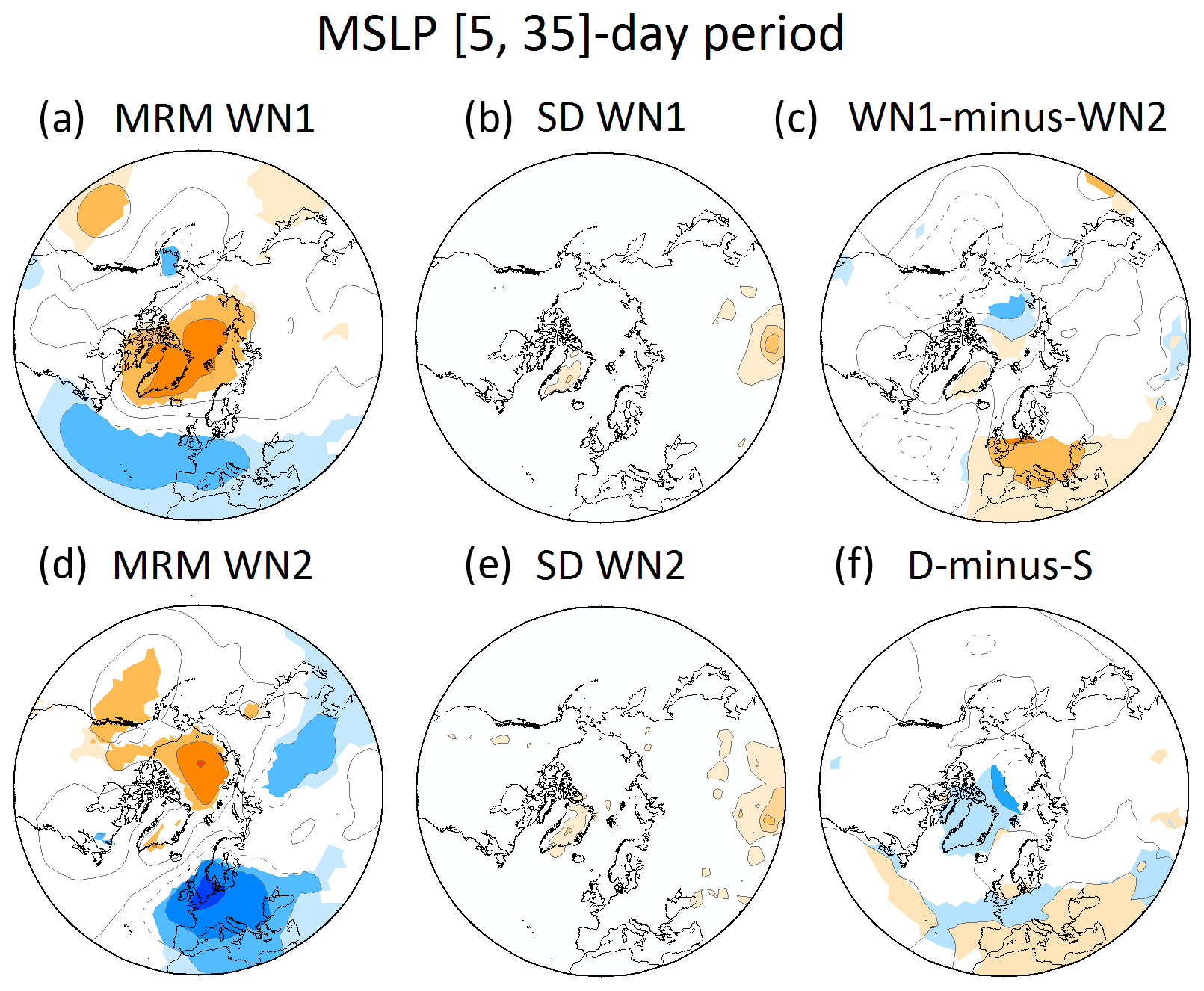
Figure 9 Same as Fig. 7 but for MSLP and the [5, 35] d period after SSWs. Contour interval is 2 hPa for MRM composites and differences and 0.1 hPa for the standard deviation of the reanalyses.

In the last decades, many studies have focused on the surface signal of D and S SSWs (e.g., Charlton and Polvani, 2007; Mitchell et al., 2013; Lehtonen and Karpechko, 2016). However, this classification is difficult to predict before the SSW onset since it is strongly based on the evolution of the polar vortex during the post-warming phase. Here, we have rather investigated the surface signal of WN1 and WN2 SSWs, whose typification is dictated by their precursors. Indeed, whereas the Z500 patterns preceding SSWs show statistically significant differences between WN1 and WN2 events (Fig. 7c), the areas with statistical significance of the differences between D and S events are more limited (Fig. 7f). In the case of the surface signal, both classifications (WN1/WN2 or S∕D) show areas of statistically significant differences between the two types of events (compare Fig. 9c and f). Our results agree well with previous studies that also found a surface signal for D and S SSWs (e.g., Charlton and Polvani, 2007; Maycock and Hitchcock, 2015). Maycock and Hitchcock (2015) indicated that the absence of a surface fingerprint for D SSWs reported by previous studies is more probably due to the sampling of events rather than a physical reason. The reported differences between the surface impacts of WN1 and WN2 SSWs may also be influenced by this issue, particularly considering the small sampling size of WN2 events. Still, our results confirm a detectable surface fingerprint for all types of SSWs independently of the classification chosen.

6 Summary and conclusions

In this study, we have compared the representation of the main features, triggering processes, and surface fingerprint of SSWs in different generations of reanalyses. Apart from a direct assessment of the SSW characteristics in the pre- and post-satellite periods, questions concerning the representation of SSWs by reanalyses have been addressed thanks to the larger number of datasets available for the post-1979 period. Unlike most studies that focus on D versus S SSWs, a separate analysis of WN1 and WN2 events has also been performed. The main conclusions are summarized as follows:

• An overall good agreement across reanalyses is found in the representation of the main features of SSWs. However, there are differences across reanalyses, particularly in the historical period, concerning the characteristics of SSWs in the middle stratosphere such as amplitude or deceleration of the PNJ. Some of the discrepancies also extend to climatological fields and their variability and are more pronounced for the NCEP-NCAR reanalysis, in agreement with Badin and Domeisen (2014). Arguably, the characteristics of the reanalysis models, including the location of their upper lid, play an important role in that period, when the performance of the reanalysis is preferentially determined by the characteristics of the underlying model. These limitations also affect the comparison period, but to a much less extent, due to the availability of satellite data in the upper levels.

• In general, SSWs (frequency, type, and dynamical benchmarks) do not substantially differ between the historical and comparison periods. Only the seasonal distribution of SSWs reveals robust differences between both periods with a shift towards a later occurrence in the satellite period, in agreement with Gómez-Escolar et al. (2012) and Hitchcock (2019).

• SSWs are mainly associated with anomalous wave packets immediately before their onset. However, the interference with climatological stationary waves plays a predominant role several days before the SSW onset. This behavior is robust across reanalyses during the comparison period, but subject to considerable uncertainties during the historical period concerning the wave activity in the middle stratosphere.

• WN1 and WN2 SSWs and their tropospheric precursors display differences in the comparison period that are robustly captured by all reanalyses. WN1 events are mainly triggered by the interaction between climatological and anomalous waves during long-lasting and moderately intense peaks of HF anomalies. Conversely, WN2 events are related to intense but short-lived pulses of HF arising from anomalous wave packets. The results resemble those by Smith and Kushner (2012) for D and S events, despite the lack of a one-to-one correspondence between WN1 (WN2) and D (S) SSWs.

• The tropospheric precursor signal shows predominant WN1-like and WN2-like structures for WN1 and WN2 SSWs, respectively. This is consistent with the spatial distribution of blockings preceding both types of SSWs. For WN1 SSWs, there is an enhanced activity over the western Atlantic and below normal frequencies over the eastern Pacific, with nearly opposite patterns for WN2 SSWs. A robust pattern emerges for all reanalyses but there are substantial differences among blocking definitions.

• Both WN1 and WN2 SSWs have significant impacts on surface weather characterized by a negative NAM pattern but with some differences in southern and central Europe. These differences are significantly different between WN1 and WN2 events and robust across reanalyses during the comparison period.

In summary, we conclude that the representation of SSWs is, in general, robust in both periods of study for the available reanalyses, and overall not different between the pre- and post-satellite eras. This would agree with Hitchcock (2019), who recommended the consideration of using data prior to 1979 in dynamical studies for stratosphere–troposphere coupling as it might be advantageous for reducing the sampling uncertainty for many purposes. However, in our study some discrepancies in the historical period were identified, particularly for the NCEP-NCAR reanalysis, which limit its use for this period in model evaluation initiatives. Furthermore, this work provides some guidelines, highlighting discrepancies among reanalyses concerning SSWs and identifying related aspects that may be sensitive to the chosen reanalysis. Although robust, some reanalyses results (such as the differences between types of SSWs) should be taken with caution in this period due to the limited sampling.