the Creative Commons Attribution 4.0 License.
the Creative Commons Attribution 4.0 License.
 | 23 Jul 2019
Predicted ultrafine particulate matter source contribution across the continental United States during summertime air pollution events
Melissa A. Venecek
Xin Yu
Michael J. Kleeman
The regional concentrations of airborne ultrafine particulate matter mass (Dp<0.1 µm; PM0.1) were predicted in 39 cities across the United States (US) during summertime air pollution episodes. Calculations were performed using a regional source-oriented chemical transport model with 4 km spatial resolution operating on the National Emissions Inventory created by the U.S. Environmental Protection Agency (EPA). Measured source profiles for particle size and composition between 0.01 and 10 µm were used to translate PM total mass to PM0.1. Predicted PM0.1 concentrations exceeded 2 µg m−3 during summer pollution episodes in major urban regions across the US including Los Angeles, the San Francisco Bay Area, Houston, Miami, and New York. PM0.1 spatial gradients were sharper than PM2.5 spatial gradients due to the dominance of primary aerosol in PM0.1. Artificial source tags were used to track contributions to primary PM0.1 and PM2.5 from 15 source categories. On-road gasoline and diesel vehicles made significant contributions to regional PM0.1 in all 39 cities even though peak contributions within 0.3 km of the roadway were not resolved by the 4 km grid cells. Cooking also made significant contributions to PM0.1 in all cities but biomass combustion was only important in locations impacted by summer wildfires. Aviation was a significant source of PM0.1 in cities that had airports within their urban footprints. Industrial sources, including cement manufacturing, process heating, steel foundries, and paper and pulp processing, impacted their immediate vicinity but did not significantly contribute to PM0.1 concentrations in any of the target 39 cities. Natural gas combustion made significant contributions to PM0.1 concentrations due to the widespread use of this fuel for electricity generation, industrial applications, residential use, and commercial use. The major sources of primary PM0.1 and PM2.5 were notably different in many cities. Future epidemiological studies may be able to differentiate PM0.1 and PM2.5 health effects by contrasting cities with different ratios of PM0.1∕PM2.5. In the current study, cities with higher PM0.1∕PM2.5 ratios (ratio greater than 0.10) include Houston, TX, Los Angeles, CA, Bakersfield, CA, Salt Lake City, UT, and Cleveland, OH. Cities with lower PM0.1 to PM2.5 ratios (ratio lower than 0.05) include Lake Charles, LA, Baton Rouge, LA, St. Louis, MO, Baltimore, MD, and Washington, D.C.
- Article
(7312 KB) - Full-text XML
-
Supplement
(1490 KB) - BibTeX
- EndNote


Airborne particulate matter (PM) has been linked with premature mortality and numerous other health risks in cities across the world (see, for example, references Dominici et al., 2006; Franklin et al., 2007; Pope et al., 2002, 2009; Ostro et al., 2006; Laden et al., 2000; Kheirbek et al., 2013; Aneja et al., 2017). Despite years of progress (EPA, 2017a), PM concentrations in many urban regions in the US still exceed health-based standards, resulting in an increase in non-accidental mortality (Franklin et al., 2007; Baxter et al., 2013). Toxicology testing suggests that ultrafine particles with a diameter <0.1 µm may be the most harmful size fraction within PM2.5 (Li et al., 2003; Oberdorster, 2000; Ostro et al., 2015; Oberdorseter et al., 1995; Pekkanen et al., 1997). Initial attempts to analyze ultrafine particles in epidemiology studies have used particle number concentration as a surrogate for ultrafine particle exposure, but this approach has not found consistent relationships with health effects (HEI, 2013). In contrast, a recent epidemiology study based on ultrafine particle mass (PM0.1) found significant associations with premature mortality (Ostro et al., 2015). In addition, ultrafine (UF) mass concentrations are highly correlated with particle surface area and can be a good metric for potential exposure to UF particles (Kuwayama et al., 2013; Ostro et al., 2015). Follow-up studies have also found significant associations between PM0.1 and reproductive outcomes, including low birth weight and preterm birth (Laurent et al., 2016; Bergin et al., 1996). These findings have biological plausibility, since ultrafine particles may cross cell membranes and interfere with internal cell function (Sioutas et al., 2005). Ultrafine particles have greater surface area per volume due to the small particle diameter, making them more available for chemical reaction. Ultrafine particles can therefore have a larger impact when deposited deep into the lung cavity, from which they are not easily removed (Nel et al., 2006; Li et al., 2003).
A monitoring network for PM10 and PM2.5 has been operating throughout the continental US for almost 20 years. Multiple studies have performed source apportionment calculations for coarse and fine PM using these measurements (see, for example, Reff et al., 2009; Zhang et al., 2014; Zheng et al., 2002; Ham and Kleeman, 2011). In contrast, measurements of PM0.1 are limited to focused field campaigns lasting for short time periods with even fewer studies attempting source apportionment calculations (Kleeman et al., 2009). Multiple barriers have prevented the widespread deployment of PM0.1 monitoring networks including (i) the low concentration of PM0.1 mass, which challenges the detection limits of analytical methods, (ii) the artifacts associated with collecting PM0.1 samples, (iii) the additional workload involved in operating the collection devices, and (iv) the sharp spatial gradients of PM0.1 concentrations. Expensive investments in PM0.1 monitoring are unlikely to be purchased without compelling evidence linking PM0.1 to public health. Early epidemiological studies for PM0.1 must therefore use techniques other than direct measurements to calculate population exposure.
Various methods, such as the source-resolved PMCAMx chemical transport model, the chemical mass balance (CMB) model, photochemical box models, and land use regression (LUR) models, have been used to track source contributions to primary organic matter, elemental carbon, and in some cases particle number concentration (Nx) over areas in the Eastern US and parts of Europe and Asia (Lane et al., 2007; Posner and Pandis, 2015; Wang et al., 2011; Cattani et al., 2017; Wolf et al., 2017; Simon et al., 2018; Gaydos et al., 2005; Zhong et al., 2018). However, these methods are limited in one or more aspects of their ability to predict population exposure to ultrafine particles over large analysis domains. Source-resolved models, such as PMCAMx, have been used to resolve composition for Nx in the Eastern US but not for PM0.1 (Posner and Pandis, 2015). CMB models need measurements of specific molecular markers at numerous sites to resolve the sharp spatial gradients of ultrafine particle source contributions. LUR models need comprehensive measurements that act as training data sets in order to extend throughout a modeling domain (Lane et al., 2007).
Hu et al. (2014) calculated population exposure to PM0.1 in California using a regional source-oriented chemical transport model supported by measured profiles for the size and composition of particles emitted by dominant sources. Predictions were compared to all available fine and ultrafine particle measurements over the period 2000–2010 with good agreement observed for the dominant chemical components of PM0.1 mass including organic aerosol, elemental carbon, and numerous trace metals (Hu et al., 2014). The 4 km spatial resolution used in these calculations supported multiple epidemiological studies based on spatial gradients of exposure (Ostro et al., 2015; Laurent et al., 2016). These encouraging results motivate the expansion of the PM0.1 exposure technique to other locations.
Here we use the Eulerian source-oriented UCD–CIT chemical transport model to predict the concentration of PM0.1 in 39 urban regions throughout the US during summer pollution events in 2010. The calculation tracks contributions from 15 primary particle sources through a simulation of all major atmospheric processes while retaining information about particle size, composition, and source origin (Hu et al., 2014). The results of this calculation reveal US national trends in PM0.1 concentrations for the first time and suggest locations where the differential health effects of PM0.1 and PM2.5 can best be studied.
2.1 Simulation dates
A total of 39 of the largest cities in the continental US were selected as the primary target locations in the current study (Fig. 1). These cities have been used to characterize atmospheric reactivity across the US in previous air pollution studies (Carter, 1994, 2010; Venecek et al., 2018a, b). Simulations within each target city were carried out during peak summer air pollution events in 2010. Dates were selected based on an initial investigation of measured 1 h ozone (O3) across all monitors in a core-based statistical area (CBSA). A CBSA is defined as a US geographical area that consists of one or more counties anchored by an urban center of at least 10 000 people plus adjacent counties that have a high degree of social and economic integration with the core as measured by commuting (United States Census Bureau, 2018).
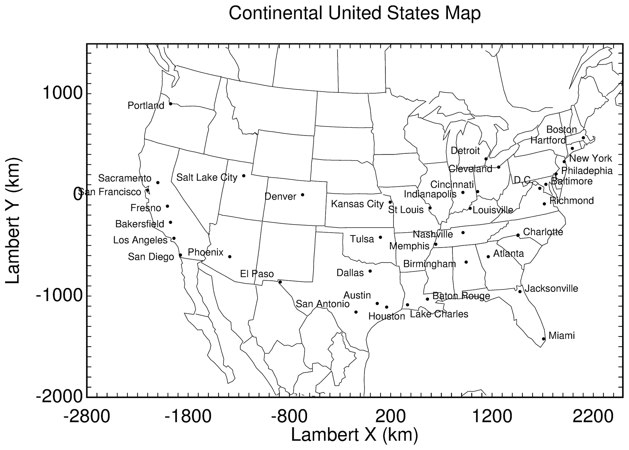
Figure 1Map of 39 cities used for the prediction of PM2.5 and PM0.1 source contributions across the continental United States during summertime air pollution events.
The selected air pollution events within each CBSA typically had measured 1 h maximum O3 concentrations greater than 70 ppb. Regional pollution events caused by atmospheric stagnation were selected whenever possible as opposed to special events caused by unusual occurrences such as wildfires that affected only one city at a time. The simulation dates in each city are listed in Table 1. Figure 2 illustrates the average 1 h maximum O3 concentration across all monitors within each CBSA during the selected regional events. Simulation periods are organized in chronological order for the year 2010, and cities within the same geographical region are grouped together. Measured 24 h PM2.5 concentrations during peak summer pollution events ranged between 3.2 and 30 µg m−3 depending on the location. The aggregation of these events across the US enables a comparison of typical summertime air pollution episodes within different cities.

Figure 2Average 1 h maximum O3 across all monitors in each domain. Cities are grouped by corresponding extreme O3 dates (that averaged >70 ppb) and US geographical region.
Table 1City, city code, simulation date, 2010 population, and geographical region.

2.2 Model description
The UCD–CIT model predicts the evolution of gas- and particle-phase pollutants in the atmosphere in the presence of emissions, transport, deposition, chemical reaction, and phase change (Held et al., 2005) as represented by Eq. (1):
where Ci is the concentration of gas- or particle-phase species i at a particular location as a function of time t, u is the wind vector, K is the turbulent eddy diffusivity, Ei is the emissions rate, Si is the loss rate, is the change in concentration due to gas-phase reactions, is the change in concentration due to particle-phase reactions, and is the change in concentration due to phase change (Held et al., 2005). Loss rates include both dry and wet deposition. Phase change for inorganic species occurs using a kinetic treatment for gas–particle conversion (Hu et al., 2008) driven towards the point of thermodynamic equilibrium (Nenes et al., 1998). Phase change for organic species is also treated as a kinetic process with vapor pressures of semi-volatile organics calculated using the two-product model (Carlton et al., 2010). More sophisticated approaches for secondary organic aerosol (SOA) formation (Cappa et al., 2016) were also tested in the current study but these required a larger number of assumptions and they did not produce higher SOA concentrations in the PM0.1 size fraction.
Nucleation was included in the model using the ternary nucleation (TN) mechanism involving H2SO4–H2O–NH3 (Napari et al., 2002). A tunable nucleation parameter equal to 10−5 was used based on results from previous studies across California for the year 2012 (Yu et al., 2019). Yu et al. (2019) found good agreement between predicted and measured concentrations of daily-averaged PM0.1 and N7 source contributions in California. The current study expands these nucleation calculations to investigate new particle formation across all major US cities, but the data needed to evaluate the accuracy of these calculations are generally not available outside California, and particle number concentrations will not be a focal point of this work. The model spatial resolution was 4 km over the 4.2 million km2 of simulated urban areas, so near-roadway concentrations of ultrafine particles on spatial scales of ∼0.1 km will not be presented.
A total of 50 particle-phase chemical species are included in each of 15 discrete particle size bins that range from 0.01 and 10 µm in particle diameter (Held et al., 2005). Artificial source tags are used to quantify source contributions to the primary particle mass and the secondary organic aerosol (SOA) mass for a specific bin size, thereby allowing the direct contribution of each source of PM2.5 and PM0.1 mass to be determined. Gas-phase concentrations of oxides of nitrogen (NOx), volatile organic compounds (VOCs), oxidants, O3, and semi-volatile reaction products were predicted using the SAPRC-11 chemical mechanism (Carter and Heo, 2013).
2.3 Model inputs
Anthropogenic emissions were generated using the Sparse Matrix Operator Kernel Emissions (SMOKEv3.7) modeling system applied to the 2011 National Emissions Inventory. The NEI reports county-wide emission totals from all 50 states that are then mapped using spatial surrogates. Temporal profiles are also used to account for variation by time of month, week, and day; however, the NEI does not account for “no-burn” days that would impact residential wood combustion or precipitation events that would impact paved–unpaved road dust. These default profiles may result in larger model performance bias when comparing predictions to measured values. Emissions from each of the four major source sectors (area, mobile, non-road, and point) were tagged to create 15 different emissions groups: on-road diesel, on-road gasoline, off-road diesel, off-road gasoline, biomass, cooking, natural gas, process heaters, distillate (oil), aviation, cement, coal, steel foundries, paper products, and all other emissions. Size- and composition-resolved source profiles were then assigned to the PM emissions within each of these groups using the UCD–CIT emissions processor based on the most recent measurements available in the literature (Robert et al., 2007a, b; Kleeman et al., 2008). Some of the 15 source categories were represented using weighted-average source profiles from multiple sources as described in Table S1 in the Supplement.
Daily values for 2010 wildfire emissions were generated using the Global Fire Emissions Database (GFED) (Giglio et al., 2013). Biogenic emission rates were generated using the Model of Emissions of Gases and Aerosols from Nature (MEGANv2.1). The gridded geo-referenced emission factors and land cover variables required for MEGAN calculations were created using the MEGANv2.1 preprocessor tool and the ESRI_GRID leaf area index and plant functional type files available at the Community Data Portal (Guenther et al., 2012).
Meteorology parameters used to drive the UCD–CIT chemical transport model (CTM) and the MEGANv2.1 biogenic emissions were generated using the Weather Research and Forecasting model (WRFv3.6) and WRF preprocessing system (WPSv3.6). Meteorological fields were created within three nested domains with horizontal resolutions of 36, 12, and 4 km. Each domain had 31 telescoping vertical levels up to a top height of 12 km. Four-dimensional data assimilation (FDDA) or “FDDA nudging” was used to anchor meteorological predictions to measured values (Hu et al., 2010). Meteorological data and gridded map projections needed for 2010 emissions modeling were taken from the corresponding WRF simulations using the meteorology–chemistry interface processor (MCIP).
2.4 Supporting measurements
Ambient hourly O3 measurements and daily PM2.5 measurements were obtained from the Environmental Protection Agency (EPA) AQS API/Query AirData (EPA, 2017b). Model predictions are compared to these measurements to build confidence in the accuracy of the overall modeling system since PM0.1 measurements are not available during any of the peak summer pollution events studied here.
Predicted maximum 1 h O3, NO2, SO2, and CO concentrations were compared to measurements at all available monitors within each study CBSA to indirectly evaluate the accuracy of the emissions inventories and meteorology fields. Many of the sources that emit O3 precursors also emit ultrafine particles. Likewise, meteorological parameters like wind speed and mixing depth influence the concentrations of all pollutants, including ultrafine particles. Successful prediction of gas-phase species is therefore a necessary step in the accurate prediction of ultrafine particle concentrations during summer photochemical smog episodes. Predicted 24 h PM2.5 concentrations were also compared to measurements at all available monitors within each study CBSA. Many of the combustion sources that emit primary particles within the PM2.5 size fraction also emit primary PM0.1 and/or precursor gases that can condense into the PM0.1 size range. The Chemical Speciation Monitoring Network (CSN) operated by the U.S. Environmental Protection Agency (EPA) measures PM2.5 mass and chemical composition at more than 260 sites throughout the US, including many of the 39 cities studied in the current analysis (Solomon et al., 2014). Full monitor information including latitude, longitude, and total number of available measurements for comparison within the simulation period are show in Tables S2–S6.
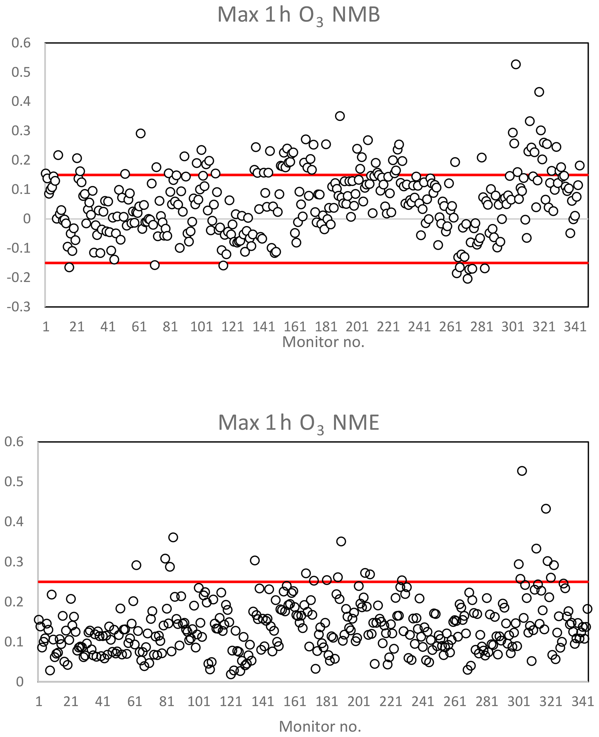
Figure 3Model performance statistics for predicted maximum 1 h O3 against measured values. The red line represents performance criteria of 0.15 for NMB and 0.25 for NME. NMB and NME were calculated for available measurements against predictions at every monitor in the CBSA based on the U.S. EPA AQ Data Mart. Monitor number (horizontal axis), latitude and longitude, name, MO, MP, NMB, NME, FB, and FE values are available for all monitors in the Supplement.
Figure 3 illustrates the normalized mean bias (NMB) and normalized mean error (NME) for predicted 1 h maximum O3 against measured 1 h maximum values for each monitor within a specific modeling domain. Figure S1 in the Supplement illustrates the fractional bias (FB) and fractional error (FE) for predicted 1 h maximum CO, NO2, and SO2 against measured 1 h maximum values. Figure 4 illustrates the NMB and NME for 24 h average predicted PM2.5 concentrations against measured 24 h average PM2.5 concentrations at each available monitor over the specific simulation period. A time series of predicted vs. measured O3 concentrations is displayed in Fig. S2.
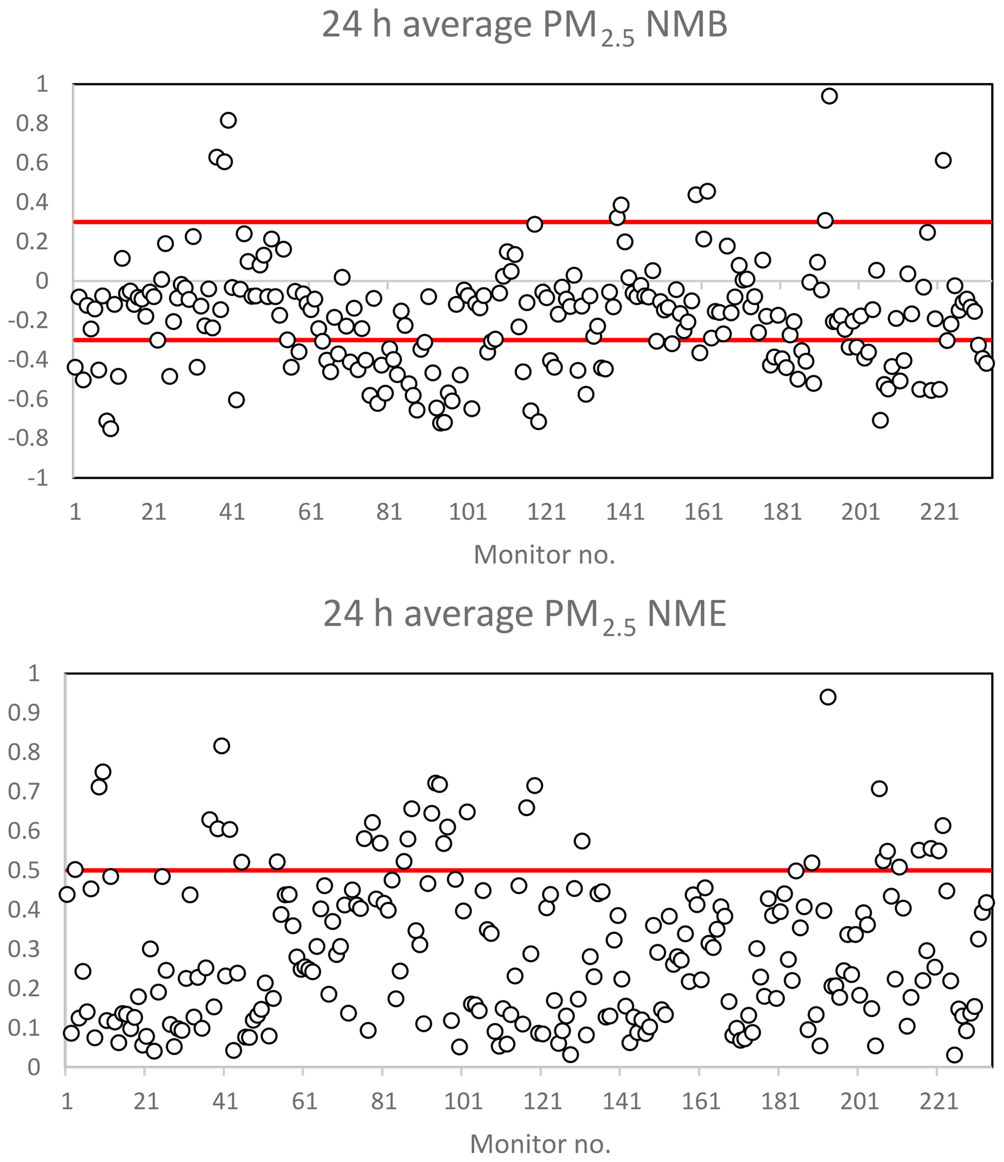
Figure 4Model performance statistics for predicted 24 h average PM2.5 against measured values. The red line represents performance criteria of ±0.30 for NMB and 0.50 for NME. Normalized mean bias and normalized mean error were calculated for available measurements against predictions at every monitor in the CBSA based on the U.S. EPA AQ Data Mart. Monitor number (horizontal axis), latitude and longitude, name, MO, MP, NMB, NME, FB, and FE values are available for all species in the Supplement.
Table 2Percent of monitors throughout the entire US domain that met performance criteria for normalized mean error (NME).
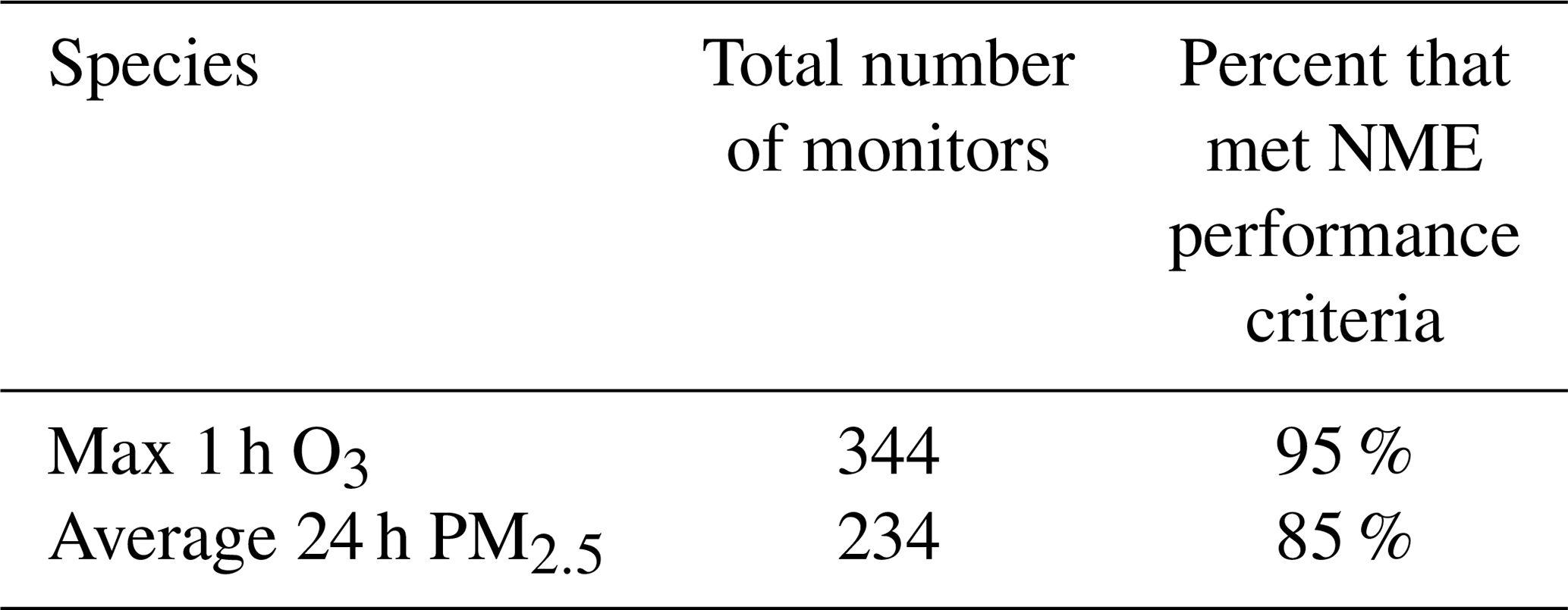
Table 2 summarizes the total number of available monitors for a comparison of measured values vs. predicted values for O3 and PM2.5. Emery et al. (2017) recommend model performance criteria for 1 h O3 NMB less than or equal to ±0.15 and NME less than or equal to 0.30. The 24 h PM2.5 model performance recommendations, also based on Emery et al. (2017), are NMB less than or equal to ±0.30 and NME less than or equal to 0.50 (Emery et al., 2017). Table 2 displays the percentage of measured vs. predicted comparisons that met the performance criteria for NME over the entire US modeling domain. In summary, 95 % of all locations met NME performance criteria for O3 predictions, and 85 % of all locations met NME performance criteria for PM2.5 predictions.
Elemental carbon (EC) and organic carbon (OC) are the chemical components most relevant for both the PM2.5 and the PM0.1 size fractions. Figure 5 illustrates predicted vs. measured 24 h PM2.5 EC and OC concentrations for all 39 cities. Primary organic matter tracked by model calculations is converted to OC by dividing by a factor of 1.2 (Russell, 2003). Secondary organic aerosol tracked by model calculations is converted to OC by dividing by a factor of 1.5. In general, the model slightly underpredicts PM2.5 EC, OC, and mass with regression slopes ranging from 0.62 for EC to 0.71 for OC. The negative bias in model predictions may stem from the 4 km spatial averaging inherent in the calculations vs. the influence of sources closer than 4 km to the measurement site in urban environments, such as highways and restaurants. Model performance statistics for PM2.5 predictions are summarized in Table S6.

Figure 5Predicted average 24 h vs. measured 24 h average (a) organic carbon and (b) elemental carbon (µg m3). Predicted OC was converted from predicted organic matter (OM) and secondary organic aerosol components using a ratio of 1.2 and 1.5, respectively (Russell, 2003).
PM0.1 measurements are not available for model evaluation in the 39 cities across the US in 2010 at the core of the current study, but measurements are available in California in the years 2015 and 2016 that can be used to evaluate similar modeling procedures. Yu et al. (2019) compared PM0.1 concentrations in Los Angeles, Fresno, East Oakland, and San Pablo, California, predicted using the UCD–CIT air quality model to receptor-based source apportionment calculations based on measured concentrations of molecular markers in the ultrafine particle size fraction (Xue et al., 2018). Good agreement was found between predictions for PM0.1 concentrations associated with gasoline engines, diesel engines, cooking, wood burning, and “other sources” from these two independent techniques. Further details on this comparison are provided by Yu et al. (2019). This evaluation of the modeling procedures builds confidence in the PM0.1 source predictions across the US in the current study, but new measurements would be helpful to fully evaluate model predictions in the future.

Figure 6(a) PM2.5 and (b) PM0.1 24 h average mass (µg m−3) during summer air pollution event. Scale drawn to highlight all areas of the US. Actual maxima: (a) 94.25 µg m−3; (b) 9.43 µg m−3.
Figure 6 illustrates a composite representation of PM2.5 and PM0.1 mass across the US during the summer pollution episodes listed in Table 1. The spatial plot in Fig. 6 is constructed using the intermediate 12 km simulation results from multiple simulations stitched together to cover a broader geographical area. Regional PM0.1 concentrations reach a maximum value of 5 µg m−3 in a few isolated grid cells with wildfires, but concentrations generally exceed 2 µg m−3 in major urban regions across the US, including Los Angeles, the San Francisco Bay Area, Houston, Miami, and New York. The comparison between PM2.5 mass (Fig. 6a) and PM0.1 mass (Fig. 6b) shows that predicted PM0.1 spatial gradients are sharper, with fewer regional contributions between “hot spots”. Locations in the Midwestern and Eastern US outside cities with high PM2.5 concentrations due to secondary formation (sulfate and secondary organic aerosol) did not have corresponding high concentrations of PM0.1. Most major urban centers had noticeable peaks of both PM2.5 and PM0.1. This pattern presents a challenge for epidemiological studies seeking to differentiate the effects of PM2.5 and PM0.1 because the locations with differential exposure (high PM2.5 but low PM0.1) have a low population density, which will reduce the power of the analysis.
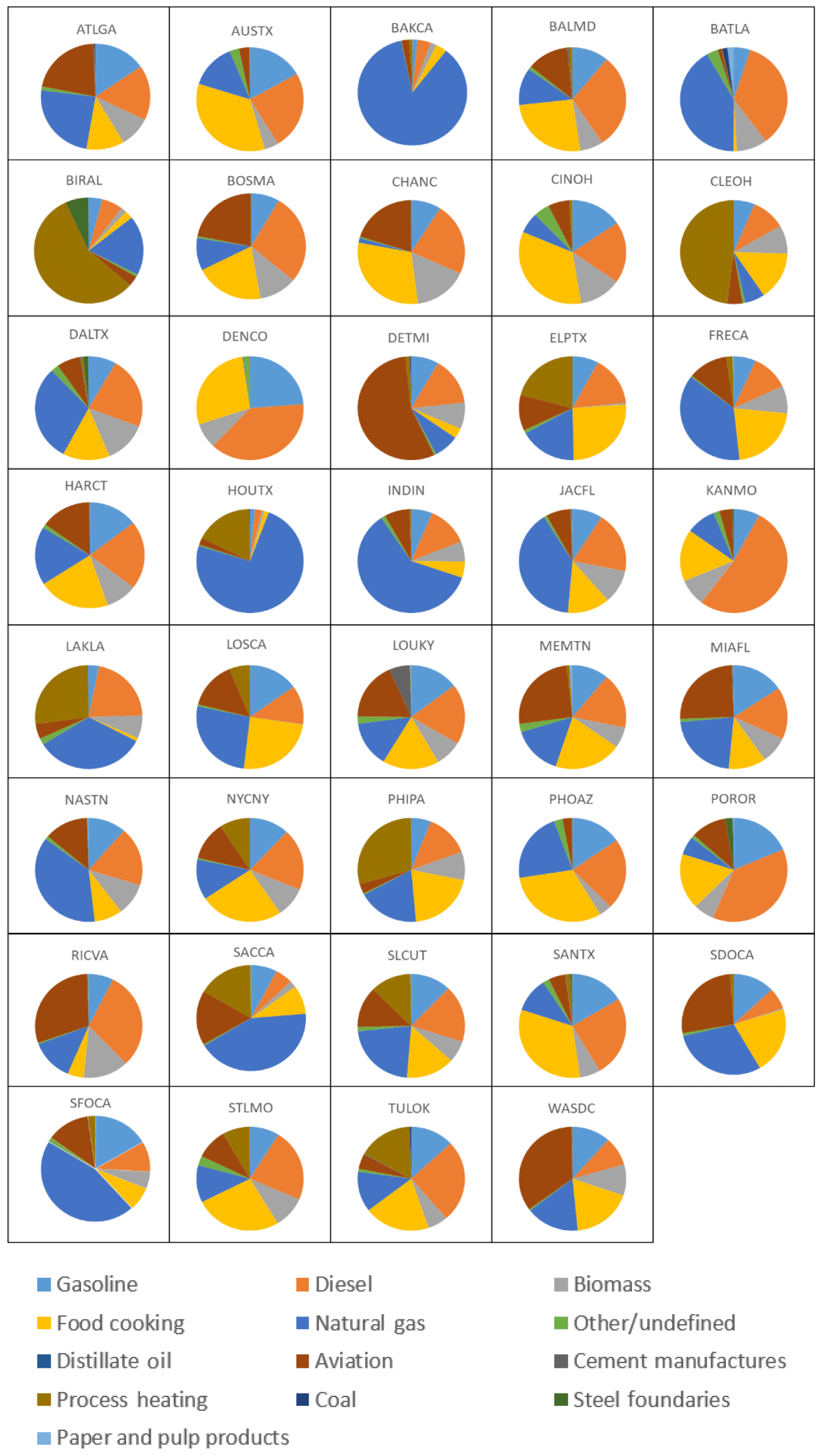
The UCD–CIT model explicitly tracks source contributions to particle mass in each size bin using artificial source tags. Pie charts of PM2.5 and PM0.1 source contributions are illustrated in Fig. 6 for selected major cities. Pie charts for PM0.1 source contributions in all 39 US cities are shown in Fig. 7. The detailed source profiles within each city are based on the nested 4 km simulation results during the pollution events listed in Table 1. Source contribution spatial plots for the entire US are shown in Figs. S3 through S5, and pie charts for PM2.5 source contributions in all 39 US cities are shown in Fig. S6. On-road gasoline and diesel vehicles made significant contributions to regional PM0.1 in all 39 cities even though peak contributions within 0.3 km of the roadway were not resolved by the 4 km grid cells. Cooking also made significant contributions to PM0.1 in all cities, but biomass combustion was only important in locations impacted by summer wildfires. Residential wood combustion is not typically a strong source in the summer due to warmer temperatures; however, in the wintertime biomass would most likely be a dominant source. Aviation was a significant source of PM0.1 in cities that have airports within their urban footprints. Industrial sources including cement manufacturing, process heating, steel foundries, and paper and pulp processing impacted their immediate vicinity but did not significantly contribute to PM0.1 concentrations in any of the target 39 cities. Natural gas combustion made significant contributions to PM0.1 concentrations due to the widespread use of this fuel for residential, commercial, and industrial applications. Natural gas contributions were especially significant in locations with high levels of industrial use, such as chemical refineries, and in locations with significant levels of natural-gas-fired power plants.
The major sources of primary PM0.1 and PM2.5 were notably different in many cities (compare Fig. 6a and b). The sources that contribute most strongly to PM2.5 are on-road diesel, gasoline, cooking, coal, and “other”, which includes brake and tire wear from mobile sources and dust. Natural gas combustion makes minor contributions to primary PM2.5 mass since particles from this source have a mass distribution peaking at ∼0.05 µm in particle diameter (Chang et al., 2004), with all of the emitted mass in the PM0.1 size fraction. In contrast, other combustion sources using more complex fuels, such as on-road vehicles, have a mass distribution peaking at ∼0.1 µm, with at least half the emitted mass outside the PM0.1 size fraction (Robert et al., 2007a, b). Likewise, cooking contributes strongly to PM2.5 concentrations, but the emitted particle mass distribution peaks at 0.2 µm, with the majority of the mass outside the PM0.1 size fraction.
The fraction of PM that is primary within each CBSA is listed in Tables S7–S16. Averaged across the US, PM2.5 was found to be approximately 62 % primary material, while PM0.1 was found to be approximately 87 % primary material.
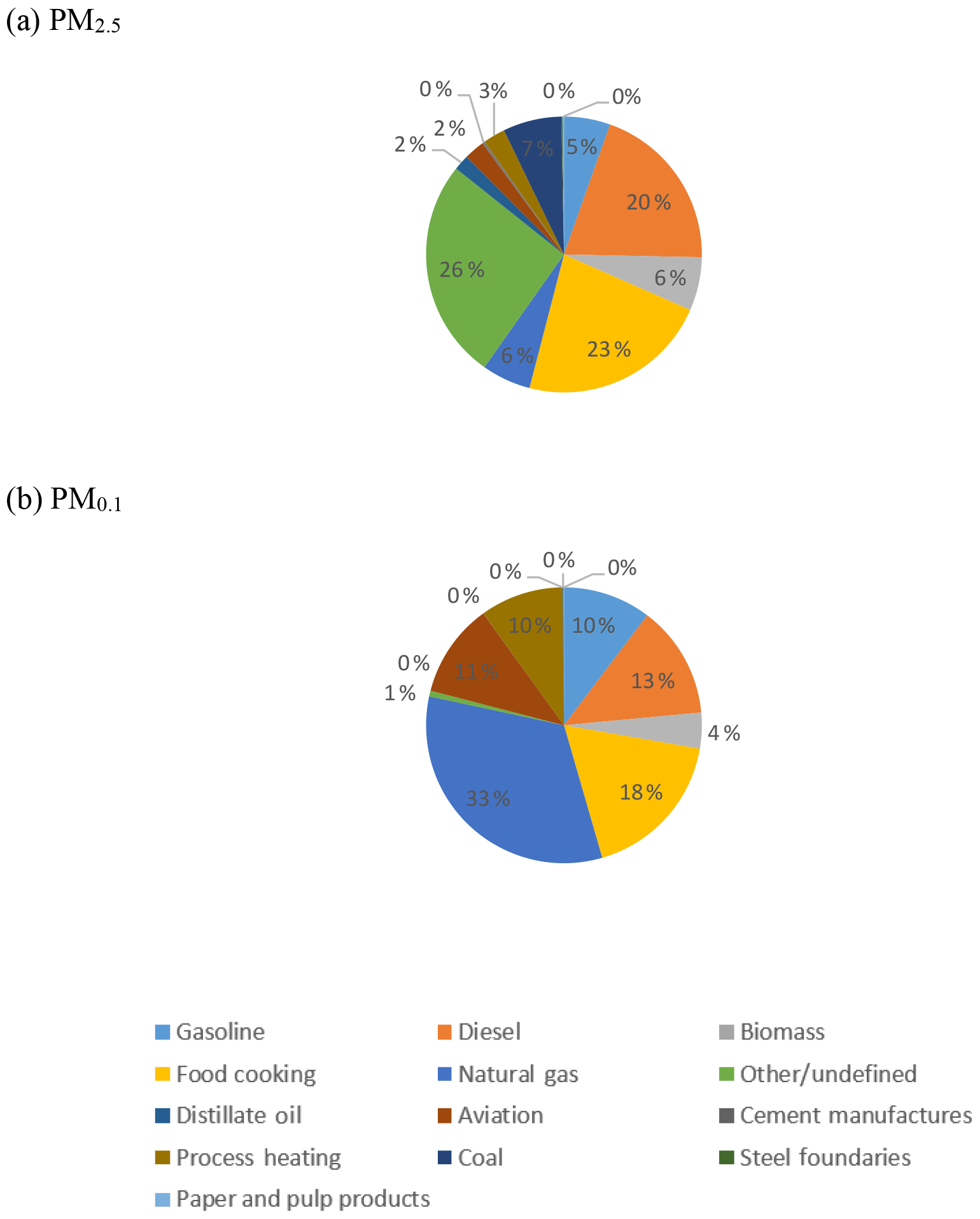
Figure 8Population-weighted average source contribution across the 39 major cities in the continental US for (a) PM2.5 and (b) PM0.1.
Figure 8 illustrates the population-weighted average PM0.1 source contributions across all 39 study cities shown in Table 1. These predictions are based on source profile measurements for wood burning, cooking, mobile sources, and nonresidential natural gas combustion reported in multiple peer-reviewed studies (Taback et al., 1979; Cooper, 1989; Houck et al., 1989; Hildemann et al., 1991a, b; Harley et al., 1992; Schauer et al., 1999a, b, 2001, 2002a, b; Kleeman et al., 2008, 2000; Robert et al., 2007a, b). In addition, new measurements made by Xue et al. (2019) were conducted to confirm previous measurements of the particle size distribution associated with natural gas and biomethane combustion particles.
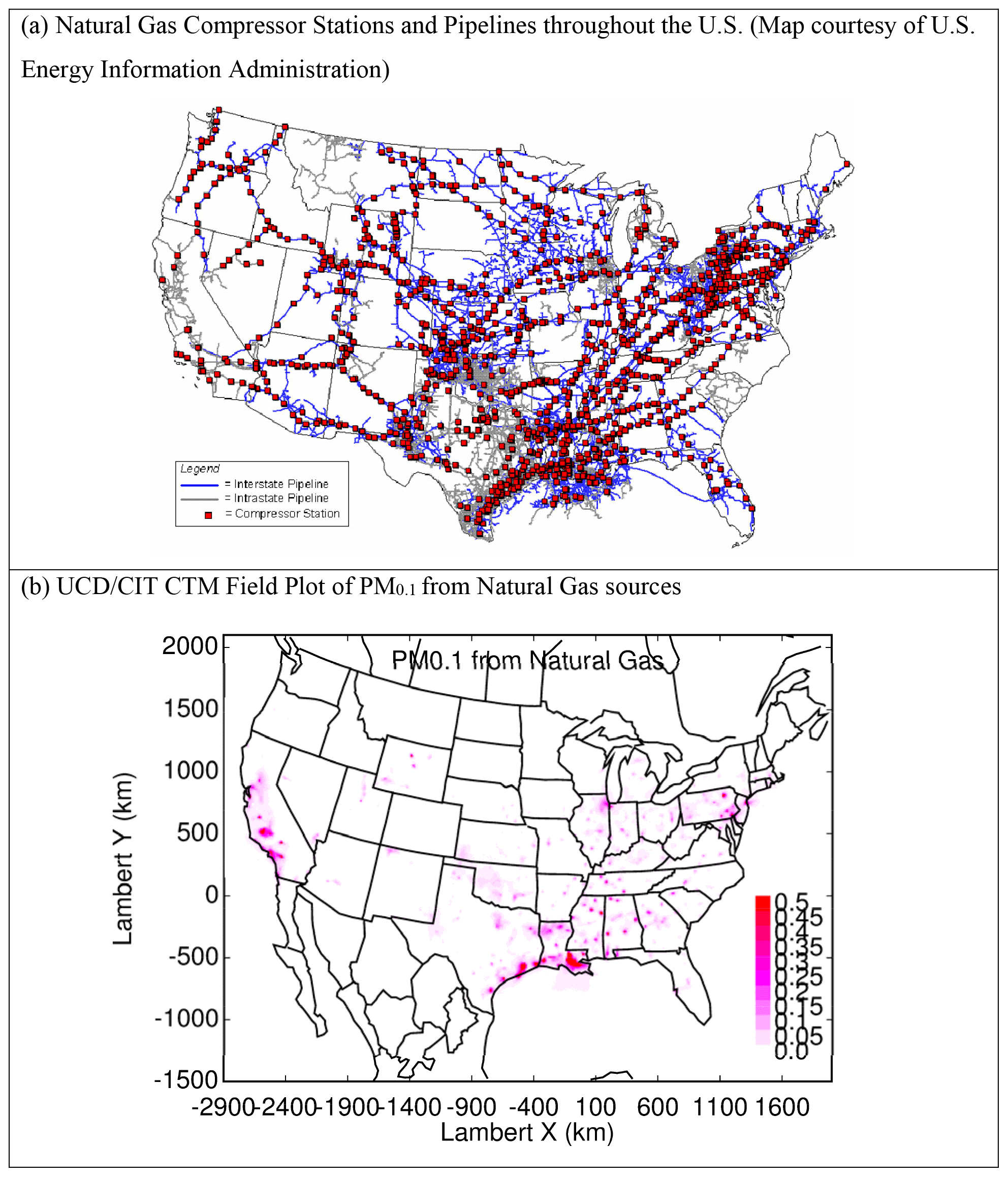
Figure 9(a) Natural gas compressor stations and pipelines across the US and (b) PM0.1 natural gas combustion concentrations (µg m−3).
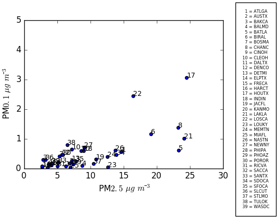
Figure 10Scatter plot showing correlation between 24 h average PM2.5 and PM0.1 for the 39 cities.
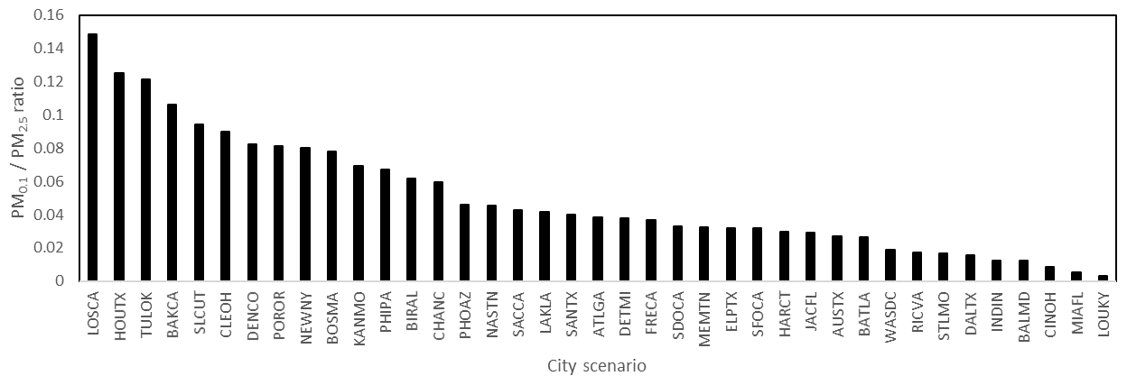
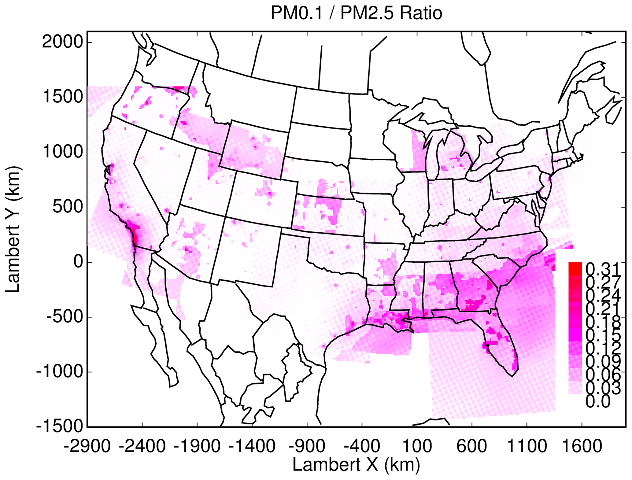
Figure 12PM0.1∕PM2.5 ratio across the US.
The results summarized in Fig. 8 highlight the importance of natural gas combustion particles in the PM0.1 size fraction and the minor role that these natural gas combustion particles play in the PM2.5 size fraction. Natural gas typically consists of +93 % methane, with the balance of the fuel made up by higher-molecular-weight alkanes and trace impurities. In addition to background sulfur compounds in the natural gas, sulfur-containing odorants such as mercaptans are commonly added to aid in leak detection. Natural gas combustion does not emit high amounts of particulate matter per joule of energy in the fuel, but the widespread use of natural gas suggests that it could still contribute significantly to ambient PM0.1 concentrations. Natural gas combustion accounted for 29 % of total US energy consumption in 2016 (U.S. Department of Energy, 2017). In contrast, gasoline combustion accounted for 17 % of US energy consumption, and diesel fuel combustion accounted for approximately 6 % of US energy consumption in 2016. Less than half of the PM emitted by gasoline and diesel fuel combustion is in the PM0.1 size fraction (Robert et al., 2007a, b), whereas all of the PM emitted by natural gas combustion is in the PM0.1 size fraction (Chang et al., 2004). Taken together, these facts support the potential importance of natural gas combustion for ambient PM0.1 concentrations.
The five states with the highest consumption of natural gas in 2016 were Texas (14.7 %), California (7.9 %), Louisiana (5.7 %), New York (5 %), and Florida (4.8 %). These consumption patterns are reflected in the natural gas distribution system (Fig. 9a) and the predicted PM0.1 concentration field associated with natural gas combustion (Fig. 9b). Natural gas end use included electric power generation (36 %), industrial applications (34 %), residential use (16 %), commercial use (11 %), and transportation (3 %).
Lane et al. (2007) used a source-resolved version of PMCAMx and individual emission inventories to determine source contributions of primary organic material (POM2.5) (Lane et al., 2007). Lane et al. (2007) note that POM2.5 associated with natural gas sources ranged from 0.1 to 0.8 µg m−3. Chang et al. (2004) measured emitted particle size distributions for gas-fired stationary combustion that fell between 10 and 100 nm. The combination of these two results indicates that the natural gas mass component of POM2.5 predicted by Lane et al. (2007) is consistent with the magnitude of the PM0.1 mass associated with natural gas combustion found in the current study. Lane et al. (2007) were not studying PM0.1, so the major role of natural gas in this size fraction was not identified.
Posner and Pandis (2015) utilized PMCAMx with the LADCO 2001 BaseE source-resolved mass emissions inventory for a July 2001 prediction of Nx over the Eastern US with 36 km resolution (Posner and Pandis, 2015). Posner and Pandis used a “zero-out” method in combination with source-specific size distribution to study the percent contribution of six major sources (on-road gasoline, industrial, non-road diesel, on-road diesel, biomass, and dust) of Nx. They found that Nx was made up of 36 % on-road gasoline, 31 % industrial, 18 % non-road diesel, 10 % on-road diesel, 1 % biomass burning, and 4 % long-range transport (Posner and Pandis, 2015). The emissions particle number inventory was normalized based on PM10 mass from each source and particle emissions from natural gas sources were assumed negligible, which effectively removed natural gas sources from the simulation. This has minor effects on PM2.5 and PM10 predictions, but the results of the current study suggest that natural gas combustion significantly contributes to ultrafine particle concentrations.
Future epidemiological studies may be able to differentiate PM0.1 and PM2.5 health effects by contrasting cities with different predicted ratios of PM0.1∕PM2.5. Although the current study does not calculate the annual average concentrations that would be needed for such an analysis, the results for the peak photochemical episodes may provide some useful insights to guide future studies. Figure 10 illustrates the correlation between predicted PM2.5 and PM0.1 concentrations in the 39 cities considered in the current analysis, Fig. 11 illustrates the ratio of PM0.1∕PM2.5 for each city, and Fig. 12 illustrates a field plot showing the ratio of PM0.1∕PM2.5 across the continental US. Cities with higher PM0.1∕PM2.5 ratios include Houston, TX, Los Angeles, CA, Salt Lake City, UT, Cleveland, OH, and Bakersfield, CA. Cities with lower PM0.1 to PM2.5 ratios include Lake Charles, LA, Baton Rouge, LA, St. Louis, MO, Baltimore, MD, and Washington, D.C. Measurements should be conducted in these locations to verify the contrast in PM0.1∕PM2.5 concentrations in preparation for future exposure analysis.
The UCD–CIT regional chemical transport model was used to predict source contributions to PM0.1 across the continental US during peak photochemical smog periods in the year 2010. Performance for PM2.5 and O3 predictions met or exceeded the criteria typically used for regional air quality model applications, building confidence in the emissions inputs and meteorological fields used to drive the calculations. Similar model exercises carried out for episodes in California in 2015 and 2016 find good agreement between predicted PM0.1 source contributions and receptor-based PM0.1 source contributions calculated using measured concentrations of molecular markers (Yu et al., 2019). In the current study, predicted regional PM0.1 concentrations exceeded 2 µg m−3 during summer pollution episodes in major urban regions across the US including Los Angeles, the San Francisco Bay Area, Houston, Miami, and New York. Predicted PM0.1 spatial gradients were sharper than predicted PM2.5 spatial gradients due to the dominance of primary aerosol in PM0.1. This finding suggests that the PM0.1 measurement networks needed to support epidemiology must be denser than comparable PM2.5 measurement networks. Nonresidential natural gas combustion was identified as a major source of PM0.1 across all major cities in the US. On-road gasoline and diesel vehicles contributed on average 14 % to regional PM0.1 even though peak contributions within 0.3 km of the roadway were not resolved by the 4 km grid cells. This is consistent with other studies that have found an exponential decrease in ultrafine particle concentrations downwind of major roadways (Wang et al., 2011) due to the sharp gradient of PM0.1. Cooking also made significant contributions to PM0.1 in all cities, but biomass combustion was only important in locations impacted by summer wildfires. Aviation was a significant source of PM0.1 in cities that have airports within their urban footprints. The major sources of primary PM0.1 and PM2.5 were notably different in many cities. Future epidemiological studies may be able to differentiate PM0.1 and PM2.5 health effects by contrasting cities with different ratios of PM0.1∕PM2.5 sources.
All of the PM0.1 and Nx outdoor exposure fields produced in the current study are available free of charge at http://faculty.engineering.ucdavis.edu/kleeman/ (last access: July 2019). The model source code and input data are available to collaborators through direct email request to the corresponding author.
The supplement related to this article is available online at: https://doi.org/10.5194/acp-19-9399-2019-supplement.
MAV prepared model input data, performed model simulations, postprocessed model output, and prepared the initial draft of the paper. XY created the nucleation module used in model calculations. MJK designed the study, created the models used for the calculations, assisted in model simulations, assisted in postprocessing model output, and revised the final paper.
The authors declare that they have no conflict of interest.
Neither CARB nor any person acting on their behalf (1) makes any warranty, express or implied, with respect to the use of any information, apparatus, method, or process disclosed in this report or (2) assumes any liabilities with respect to the use and/or damages resulting from the use or inability to use any information, apparatus, method, or process disclosed in this report.
This research was supported by the California Air Resources Board under project no. 14-314.
This research has been supported by the California Air Resources Board (grant no. 14-314).
This paper was edited by Veli-Matti Kerminen and reviewed by three anonymous referees.
Aneja, A. P., Pillai, P. R., Isherwood, A., Morgan, P., and Aneja, S. P.: Particulate matter pollution in the coal-producing regions of the Appalachian Mountains: Integrated ground-based measurements and satellite analysis, J. Air Waste Manage. Assoc., 67, 421–430, 10.1080/10962247.2016.1245686, 2017.
Baxter, L. K., Duvall, R. M., and Sacks, J.: Examining the effects of air pollution composition on within region differences in PM2.5 mortality risk estimates, J. Expo. Sci. Environ. Epidemiol., 23, 457–465, https://doi.org/10.1038/jes.2012.114, 2013.
Bergin, M. S., Russell, A. G., Yang, Y. J., Milford, J. B., Kirchner, F., and Stockwell, W. R.: Effects of uncertainty in SAPRC90 rate constants and selected product yields on reactivity adjustment facorts for alternamtive fuel vehicle emissions, Final Report, California Air Resources Board, Sacramento, CA, 1996.
Cappa, C. D., Jathar, S. H., Kleeman, M. J., Docherty, K. S., Jimenez, J. L., Seinfeld, J. H., and Wexler, A. S.: Simulating secondary organic aerosol in a regional air quality model using the statistical oxidation model – Part 2: Assessing the influence of vapor wall losses, Atmos. Chem. Phys., 16, 3041–3059, https://doi.org/10.5194/acp-16-3041-2016, 2016.
Carlton, A. G., Bhave, P. V., Napelenok, S. L., Edney, E. D., Sarwa, G., Pinder, R. W., Pouliot, G. A., and Houyoux, M.: Model representation of secondary organic aerosol in CMAQv4.7, Environ. Sci. Technol., 44, 8553–8560, 2010.
Carter, W. P. L.: Calculation of Reactivity Scales Using an Updated Carbon Bond IV Mechanism, Report Prepared for Systems Applications Internation for the Auto/Oil Air Quality Improvement Program, California Air Resources Board, Sacramento, CA, available at: https://ww3.arb.ca.gov/research/reactivity/research.htm (last access: 20 July), 1994.
Carter, W. P. L.: Development of the SAPRC-07 chemical mechanism, Atmospheric Enviornment, 44, 5324-5335, 2010.
Carter, W. P. L. and Heo, G.: Development of Revised SAPRC Aromatics Mechanisms, Atmos. Environ., 77, 404–414, 2013.
Cattani, G., Gaeta, A., Di Menno di Bucchianico, A., De Santis, A., Gaddi, R., Cusano, M., Ancona, C., Badaloni, C., Forastiere, F., Gariazzo, C., Sozzi, R., Inglessis, M., Silibello, C., Salvatori, E., Manes, F., and Cesaroni, G.: Development of land-use regression models for exposure assessment to ultrafine particles in Rome, Italy, Atmos. Environ., 156, 52–60, 2017.
Chang, M.-C., Chow, J. C., Watson, J. G., Hopke, P. K., Yi, S.-M., and England, G. C.: Measurement of Ultrafine Particle Size Distributions from Coal-, Oil-, and Gas-Fired Stationary Combustion Sources, J. Air Waste Manage. Assoc., 54, 1494–1505, https://doi.org/10.1080/10473289.2004.10471010, 2004.
Cooper, J. A.: PM10 Source composition library for the South Coast Air Basin, Appendix V-G for South Coast Air Quality Management District, South Coast Air Quality Management District, Diamond Bar ,CA, 1989.
Dominici, F., Peng, R. D., Bell, M. L., Pham, L., McDermott, A., Zeger, S. L., and Samet, J. M.: Fine Particulate Air Pollution and Hospital Admission for Cardiovascular and Respiratory Diseases, JAMA, 295, 1127–1134, https://doi.org/10.1001/jama.295.10.1127, 2006.
Emery, C., Liu, Z., Russell, A. G., Odman, M. T., Yarwood, G., and Kumar, N.: Recommendations on statistics and benchmarks to assess photochemical model performance, J. Air Waste Manage. Assoc., 67, 582–598, 2017.
Franklin, M., Zeka, A., and Schawrtz, J.: Association between PM2.5 and all-cause and specific-cause moratlity in 27 US communities, J. Expo. Sci. Env. Epid., 17, 279–287, 2007.
Gaydos, T. M., Stanier, C. O., and Pandis, S. N.: Modeling of in situ ultrafine atmospheric particle formation in the eastern United States, J. Geophys. Res., 110, D07S12, https://doi.org/10.1029/2004JD004683, 2005.
Giglio, L., Randerson, J. T., and van der Werf, G. R.: Analysis of daily, monthly and annual burned area using the fourth-generation global fire emissions database (GFED4), J. Geophys. Res., 118, 317–328, 2013.
Guenther, A. B., Jiang, X., Heald, C. L., Sakulyanontvittaya, T., Duhl, T., Emmons, L. K., and Wang, X.: The Model of Emissions of Gases and Aerosols from Nature version 2.1 (MEGAN2.1): an extended and updated framework for modeling biogenic emissions, Geosci. Model Dev., 5, 1471–1492, https://doi.org/10.5194/gmd-5-1471-2012, 2012.
Ham, W. A. and Kleeman, M. J.: Size-resolved source apportionment of carbonaceous particulate matter in urban and rural sites in central California, Atmos. Environ., 45, 3988–3995, 2011.
Harley, R. A., Hannigan, M. P., and Cass, G. R.: Respeciation of Organic Gas Emissions and the Detection of Excess Unburned Gasoline in the Atmosphere, Environ. Sci. Technol., 26, 2395–2408, 1992.
HEI: Understanding the Health Effects of Ambient Ultrafine Particles HEI Review Panel on Ultrafine Particles, Health Effects Institute Boston, MA, 2013.
Held, T., Ying, Q., Kleeman, M., Schauer, J., and Fraser, M.: A comparision of the UCD/CIT air quality model and the CMB source-receptor model for primary airborne particulate matter, Atmos. Environ., 39, 2281–2297, 2005.
Hildemann, L. M., Markowski, G. R., and Cass, G. R.: Chemical Composition of Emissions from Urban Sources of Fine Organic Aerosols, Environ Sci. Technol., 25, 744–759, 1991a.
Hildemann, L. M., Markowski, G. R., Jones, M. C., and Cass, G. R.: Sub-micrometer Aerosol Mass Distributions of Emissions from Boilers, Fireplaces, Automobiles, Diesel Trucks and Meat Cooking Operations, Aerosol Sci. Technol., 14, 138–152, 1991b.
Houck, J. E., Chow, J. C., Watson, J. G., Simmons, C. A., Prichett, L. C., and Frazier, C. A.: Determination of particle size distribution and chemical composition of particulate matter from selected sources in Califorina, California Air Resources Board, OMNI Environment Service Incorporate, California Air Resources Board, Sacramento, CA, 1989.
Hu, J., Ying, Q., Chen, J., Mahmud, A., Zhao, Z., Chen, S., and Kleeman, M. J.: Particulate air quality model predictions using prognositc vs diagnostic meteorology in central California, Atmos. Enviorn., 44, 215–226, 2010.
Hu, J., Zhang, H., Chen, S., Wiedinmyer, C., Vanderbergh, F., Ying, Q., and Kleeman, M. J.: Predicting Primary PM2.5 and PM0.1 Trace Composition for Epidemiological Studies in California, Environ. Sci. Technol., 48, 4971–4979, 2014.
Hu, X.-M., Zhang, Y., Jacobson, M. Z., and Chan, C. K.: Coupling and evaluating gas/particle mass transfer treatements for aerosol simulation and forecast, J. Geophys. Res., 113, D11208, https://doi.org/10.1029/2007Jd009588, 2008.
Kheirbek, I., Wheeler, K., Walters, S., Kass, D., and Matte, T.: PM2.5 and Ozone health impacts and disparities in New York City: sensitivity to spatial and temporal resolution, Air Qual. Atmos. Health, 6, 473–486, https://doi.org/10.1007/s11869-012-0185-4, 2013.
Kleeman, M. J., Schauer, J. J., and Cass, G. R.: Size and composition distribution of fine particulate matter emitted from motor vehicles, Environ. Sci. Technol., 34, 1132–1142, 2000.
Kleeman, M. J., Robert, M. A., Riddle, S. G., Fine, P. M., Hays, M. D., Schuaer, J. J., and Hannigan, M. P.: Size distribution of trace organic species emitted from biomass combustion and meat charbroiling, Atmos. Environ., 42, 3059–3075, 2008.
Kleeman, M. J., Riddle, S. G., Robert, M. A., Jakober, C. A., Fine, P. M., Hays, M. D., Schauer, J. J., and Hannigan, M. P.: Source Apportionment of Fine (PM1.8) and Ultrafine (PM0.1) Airborne Particulate Matter during a Severe Winter Pollution Episode, Environ. Sci. Technol., 43, 272–279, 2009.
Kuwayama, T., Ruehl, C., and Kleeman, M. J.: Daily trends and source apportionment of ultrafine particulate mass (PM0.1) over an annual cycle in a typical California City, Environ. Sci. Technol., 47, 13957–13966, 2013.
Laden, F., Neas, L. M., Docker, D. W., and Schwarts, J.: Association of fine particulate matter from different sources with daily mortality in six U.S. Cities, Environ. Health Persp., 108, 941–947, 2000.
Lane, T. E., Pinder, R. W., Shrivastava, M., Robinson, A. L., and Pandis, S. N.: Source contributions to primary organic aerosol: Comparison of the results of a source-resolved model and the chemical mass balance approach, Atmos. Environ., 41, 3758–3776, 2007.
Laurent, O., Hu, J., Li, L., Kleeman, M. J., Bartell, S. M., Cockburn, M., Escobedo, L., and Wu, J.: A Statewide Nested Case-Control Study of Preterm Birth and Air Pollution by Source and Composition: California, 2001–2008, Environ. Int., 92–92, 471–477, https://doi.org/10.1289/ehp.1510133, 2016.
Li, N., Siotas, C., Cho, A., Schmitz, D., Misra, C., J., S., Wang, M. Y., Oberley, T., Froines, J., and Nel, A.: Ultrafine particulate pollutants induce oxidative stress and mitochondrial damage, Environ. Health Persp., 111, 455–460, 2003.
Napari, I., Noppel, M., Vehkamaki, H., and Kulmala, M.: Parametrization of ternary nucleation rates for H2SO4-NH3-H2O vapors, J. Geophys. Res.-Atmos., 107, 4381, https://doi.org/10.1029/2002JD002132, 2002.
Nel, A., Xia, T., Madler, L., and Li, N.: Toxic potential of materials at the nanolevel, Science, 311, 622–627, 2006.
Nenes, A., Pilinis, C., and Pandis, S. N.: ISORROPIA: A new thermodynamic equilibrium model for multiphase multicomponent marine aerosols, Aquat. Geochem., 4, 123–152, 1998.
Oberdorster, G.: Toxicology of ultrafine particles: in vivo studies, The Royal Society, 358, https://doi.org/10.1098/rsta.2000.0680, 2000.
Oberdorseter, G., Gelein, R., Ferin, J., and Weiss, B.: Association of Particulate Air Pollution and ACute Mortality: Involvement of Ultrafine Particles, Inhal. Toxicol., 7, 111–124, 1995.
Ostro, B., Broadwin, R., Green, S., Feng, W. Y., and Lipsett, M.: Fine particulate air pollution and mortality in nine California counties: Results from CALFINE, Environ. Health Persp., 114, 29–33, 2006.
Ostro, B., Hu, J., Goldber, D., Reynolds, P., Hertz, A., Bernstein, L., and Kleeman, M. J.: Associations of mortality with long-term exposures to fine and ultrafine particles, species and sources: results from the California Teachers Study Cohort, Environ. Health Persp., 123, 549–556, 2015.
Pekkanen, J., Timonen, K. L., Ruuskanen, J., Reponen, A., and Mirme, A.: Effects of Ultra-Fine and fine PArticles in Uran Air on Peak Expiratory Flow Among Children with Asthmatic Symptoms, Environ. Res., 74, 24–33, 1997.
Pope, C. A., Burnett, R. T., Thun, M. J., Calle, E. E., Krewski, D., Ito, K., and Thursdton, G. D.: Lung Cancer, Cardiopulmonary Mortality and Long Term Exposer to Fine Particulate Air Pollution, JAMA-J. Am. Med. Assoc., 287, 1132–1141, 2002.
Pope, C. A., Ezzati, M., and Dockery, D. W.: Fine-Particulate Air Pollution and US County Life Expectancies, New Engl. J. Med., 360, 376–386, 2009.
Posner, L. A. and Pandis, S. N.: Sources of ultrafine particles in the Eastern United States, Atmos. Environ., 111, 103–112, 2015.
Reff, A., Bhave, P. V., Simon, H., Pace, T. G., Pouliot, G. A., Mobley, J. D., and Houyoux, M.: Emissions Inventory of PM2.5 Trace Elements across the United States, Environ. Sci. Technol., 43, 5790–5796, 2009.
Robert, M. A., Kleeman, M. J., and Jakober, C. A.: Size and composition distrubtions of particulate matter emissions: Part 2 – Heavy-duty diesel vehicles, J. Air Waste Manage. Assoc., 57, 1429–1438, 2007a.
Robert, M. A., VanBergen, S., Kleeman, M. J., and Jakober, C. A.: Size and Composition distributions of particulate matter emissions: Part 1 – Light duty gasoline vehciles, J. Air Waste Manage. Assoc., 57, 1414–1428, 2007b.
Russell, L. M.: Aerosol organic-mass-to-organic-carbon ratio measurements, Environ. Sci. Technol., 37, 2982–2987, 2003.
Schauer, J. J., Kleeman, M. J., Cass, G. R., and Simoneit, B. R. T.: Measurement of emissions from air pollution sources C-1 through C-29 organic compounds from meat charbroiling, Environ. Sci. Technol., 33, 1566–1577, 1999a.
Schauer, J. J., Kleeman, M. J., Cass, G. R., and Simoneit, B. R. T.: Measurments of emissions from air pollution sources 2. C-1 through C30 organic compounds from medium duty diesel trucks, Environ. Sci. Technol., 33, 1578–1587, 1999b.
Schauer, J. J., Kleeman, M. J., Cass, G. R., and Simoneit, B. R. T.: Measurement of emissions from air pollution sources 3. C-1-C-29 organic compounds from fireplace combustion of wood, Environ. Sci. Technol., 35, 1716–1728, 2001.
Schauer, J. J., Kleeman, M. J., Cass, G. R., and Simoneit, B. R. T.: Measurement of emissions from air pollution sources 4. C-1-C-27 organic compounds from cooking with seed oils, Environ. Sci. Technol., 36, 567–575, 2002a.
Schauer, J. J., Kleeman, M. J., Cass, G. R., and Simoneit, B. R. T.: Measurment of emissions from air pollution sources 5. C-1-C-32 organic compounds from gasoline powered motor vehicles, Environ. Sci. Technol., 36, 1169–1180, 2002b.
Simon, M. C., Patton, A. P., Naumova, E. N., Levy, J. I., Kumar, P., Brugge, D., and Durant, J. L.: Combining Measurements from Mobile Monitoring and a Reference Site to Develop Models of Ambient Ultrafine Particle Number Concentrations at Residences, Environ. Sci. Technol., 52, 6985–6995, 2018.
Sioutas, C., Delfino, R. J., and Singh, M.: Exposure assessment for atmospheric ultrafine particles (UFPs) and implications in epidemiologic research, Environ. Health Persp., 113, 947–955, 2005.
Solomon, P. A., Crumpler, D., Flanagan, J. B., Jayant, R. K. M., Rickman, E. E., and McDade, C. E.: U.S. National PM2.5 Chemical Speciation Monitoring Networs – CSN and IMPROVE: Description of networks, J. Air Waste Manage. Assoc., 64, 1410–1438, 2014.
Taback, H. J., Brienza, A. R., Macko, J., and Brunetz, N.: Fine particle emissions from stationary and miscellaneous sources in the South Coast Air Basin, KVB Incorporated, Tustin, California, 1979.
U.S. Energy Information Administration: Natural Gas Explained, Use of Natural Gas, available at: https://www.eia.gov/energyexplained/index.php?page=natural_gas_use (last access: 1 August 2018), 2017.
U.S. Environmental Protection Agency: Air Quality Designations for Particle Pollution, available at: https://www.epa.gov/pm-pollution/forms/contact-us-about-particulate-matter-pm-pollution (last access: 24 October 2018), 2017a.
U.S. Environmental Protection Agency: AQS API/Query AirData, available at: http://aqs.epa.gov/api (last access: 24 October 2018), 2017b.
United States Census Bureau: Geographic Terms and Concepts – Core Based Statistical Areas and Related Statistical Areas, available at: https://www.census.gov/geo/reference/gtc/gtc_cbsa.html last access: 21 December 2018.
Venecek, M. A., Cai, C., Kaduwela, A., Avise, J., Carter, W. P. L., and Kleeman, M. J.: Analysis of the SAPRC16 Chemical Mechanism for Ambient Simulations, Atmos. Environ., 192, 136–150, 2018a.
Venecek, M. A., Carter, W. P. L., and Kleeman, M. J.: Updating the SAPRC Maximum Incremental Reactivity (MIR) Scale for the United States from 1988 to 2010, J. Air Waste Manage. Assoc., 68, 1301–1316, 2018b.
Wang, Y., Hopke, P. K., Chalupa, D. C., and Utell, M. J.: Long-term study of urban ultrafile particles and other pollutants, Atmos. Environ., 45, 7672–7680, 2011.
Wolf, K., Cyrys, J., Harcinikova, T., Gu, J., Kusch, T., Hampel, R., Schneider, A., and Peters, A.: Land use regression modeling of ultrafine particles, ozone, nitrogen oxides and markers of particulate matter pollution in Augsburg, Germany, Sci. Total Environ., 579, 1531–1540, 2017.
Xue, J. Xue, W., Sowlat, M. Sioutas, C., Lilinco, A., Hasson, A., and Kleeman, M.J. Seasonal and Annual Source Apportionment of Carbonaceous Ultrafine Particulate Matter (PM0.1) in Polluted California Cities. Environ. Sci. Technol., 53, 39–49, 2019.
Xue, J., Xue, W., Sowlat, M. H., Sioutas, C., Lolinco, A., Hasson, A., and Kleeman, M. J.: Seasonal and Annual Source Appointment of Carbonaceous Ultrafine Particulate Matter (PM0.1) in Polluted California Cities, Environ. Sci. Technol., 53, 39–49, https://doi.org/10.1021/acs.est.8b04404, 2019.
Yu, X., Venecek, M., Hu, J., Tanrikulu, S., Soon, S.-T., Cuong, T., Fairley, D., and Kleeman, M. J.: Regional Ultrafine Particle Number and Mass Concentrations in California, Atmos. Chem. Phys. Discuss., submitted, 2019.
Zhang, H., Hu, J., Kleeman, M., and Ying, Q.: Source apportionment of sulfate and nitrate partiulate matter int he Eastern United States and Effectiveness of emission control programs, Sci. Total Environ., 490, 171–181, 2014.
Zheng, M., Cass, G. R., Schaure, J. J., and Edgerton, E. S.: Source Apportionment of PM2.5 in the Southeastern United States Using Solvent-Extractable Organic Compounds as Tracers, Environ. Sci. Technol., 36, 2361–2371, 2002.
Zhong, J., Nikolova, I., Cai, X., MAcKenzie, A. R., and Harrison, R. M.: Modelling traffic-induced multicomponent ultrafine particles in urban street canyon compartments: Factors that inhibit mixing, Environ. Pollut., 238, 186–195, 2018.