Aerosol influences on low-level clouds in the West African monsoon

Low-level clouds (LLCs) cover a wide area of southern West Africa (SWA) during the summer monsoon months and have an important cooling effect on the regional climate. Previous studies of these clouds have focused on modelling and remote sensing via satellite. We present the first comprehensive set of in situ measurements of cloud microphysics from the region, taken during June–July 2016, as part of the DACCIWA (Dynamics–aerosol–chemistry–cloud interactions in West Africa) campaign. This novel dataset allows us to assess spatial, diurnal, and day-to-day variation in the properties of these clouds over the region.

LLCs developed overnight and mean cloud cover peaked a few hundred kilometres inland around 10:00 local solar time (LST), before clouds began to dissipate and convection intensified in the afternoon. Regional variation in LLC cover was largely orographic, and no lasting impacts in cloud cover related to pollution plumes were observed downwind of major population centres.

The boundary layer cloud drop number concentration (CDNC) was locally variable inland, ranging from 200 to 840 cm⁻³ (10th and 90th percentiles at standard temperature and pressure), but showed no systematic regional variations. Enhancements were seen in pollution plumes from the coastal cities but were not statistically significant across the region. A significant fraction of accumulation mode aerosols, and therefore cloud condensation nuclei, were from ubiquitous biomass burning smoke transported from the Southern Hemisphere.

To assess the relative importance of local and transported aerosol on the cloud field, we isolated the local contribution to the aerosol population by comparing inland and offshore size and composition measurements. A parcel model sensitivity analysis showed that doubling or halving local emissions only changed the calculated cloud drop number concentration by 13 %–22 %, as the high background meant local emissions were a small fraction of total aerosol. As the population of SWA grows, local emissions are expected to rise. Biomass burning smoke transported from the Southern Hemisphere is likely to dampen any effect of these increased local emissions on cloud–aerosol interactions. An integrative analysis between local pollution and Central African biomass burning emissions must be considered when predicting anthropogenic impacts on the regional cloud field during the West African summer monsoon.

1 Introduction

During the summer monsoon in June–September, large areas of southern West Africa (SWA) are covered by low-level clouds (LLCs), which form overnight and thicken in the morning, before breaking up in the early afternoon (van der Linden et al., 2015). By presenting a high albedo surface close to the ground, these clouds generate a strong surface cooling. Many climate models struggle to accurately represent LLCs (Hannak et al., 2017), and measurements of LLCs (and their radiative interactions with higher-level cloud layers) are a key uncertainty in the quantification of the overall cloud radiative effect in SWA (Hill et al., 2018). Most of the population centres in SWA are located near the coast, and plumes of local anthropogenic pollution are transported inland (Deroubaix et al., 2019), potentially being entrained into cloud base. Over the coming decades, the population of SWA is expected to undergo large increases (United Nations, 2017), leading to corresponding increases in emissions of anthropogenic pollution (Liousse et al., 2014). Such increases may affect dynamics and cloud microphysics in the region, and it is therefore of interest to determine any impact on the regional climate such as changes in cloud cover and precipitation (Knippertz et al., 2015b).

The DACCIWA (Dynamics–aerosol–chemistry–cloud interactions in West Africa) project (Knippertz et al., 2015a) was developed to provide a comprehensive overview of cloud–aerosol–precipitation interactions in the region. The program studied different scales, from local emission measurements near source to regional sampling using aircraft, remote sensing, and model analyses. This study focuses mostly on in situ cloud measurements made during the DACCIWA aircraft campaign (Flamant et al., 2018b), which took place between 29 June and 16 July 2016. Three research aircraft, each equipped with a suite of atmospheric measurement probes, were based out of Lomé, Togo, and conducted 50 research sorties flying over Togo, Benin, Ghana, and Côte d'Ivoire, of which 33 included in situ sampling of cloud properties.

The flying campaign took place in typical, post-onset West African monsoon conditions (Knippertz et al., 2017). In the daytime continental boundary layer, the southwesterly monsoon flow dominates the wind field, particularly in the lower kilometre of the atmosphere. Above around 1.5–2 km, the wind direction shifts to easterly, and some easterly waves and vortices passed through the region during the study period (Knippertz et al., 2017). Near the coast, winds are slowed by boundary layer turbulence, generating sea breeze clouds along a convergence front that moves up to a few tens of kilometres inland during the day (Adler et al., 2017; Deetz et al., 2018b; Flamant et al., 2018a). As the turbulence subsides in the evening, the monsoon flow strengthens to bring this front inland as the nocturnal low-level jet (NLLJ), a strong flow of cool and humid maritime air, often penetrating over 180 km inland (e.g. Kalthoff et al., 2018). We follow the convention of Adler et al. (2019) in referring to the various flows bringing marine air inland as the Gulf of Guinea maritime inflow, or simply maritime inflow for short.

The NLLJ appears to be a key factor for initiating the formation of nocturnal LLCs, and previous studies have suggested several factors may be at play, including the transport of moisture and cold air inland and the impact this has on factors such as turbulence and the radiation budget. Recent studies by Babić et al. (2019) and Adler et al. (2019) suggest the main factor may be the cooling effect of a current of cold air moving inland. The importance of the maritime inflow in cooling a particular location means that orography plays a significant role in determining geographical variation in the cloud field. Higher LLC coverage is found on the leeward side of slopes, where the maritime flow can reach more easily, and where this flow is also forced to rise orographically (van der Linden et al., 2015).

Deetz et al. (2018b) modelled the effects of changing aerosol emissions on the cloud fields in SWA. They suggested that the reduction of the land–sea temperature gradient from increasingly hazy conditions led to a weakening of the monsoon flow and nocturnal low-level jet, as well as a delay in stratocumulus to cumulus transition and cloud breakup. Haslett et al. (2019b) recently described the aerosol properties measured during the DACCIWA aircraft campaign and showed that a large background of transported biomass burning pollution from the Southern Hemisphere was ubiquitous in the West African boundary layer. Although city emissions resulted in aerosol load increases directly downwind of urban conglomerates (Brito et al., 2018), the injection of aerosols prone to activate as cloud nuclei ($>\sim \mathrm{0.1}$ µm) is thought to have limited impact on an already elevated background. This transported biomass burning background was reproducible in a modelling study by Menut et al. (2018). Painemal et al. (2014) showed that cloud–aerosol interactions with biomass burning smoke were the main factor governing cloud microphysical properties in clouds north of 5^∘ S over the South Atlantic, but so far no study has measured the microphysical properties of clouds over SWA to quantify the relative influences of transported pollution and local anthropogenic aerosol emissions.

The objectives of this paper are listed as follows.

1. Provide a statistical overview of in situ cloud properties measured during the DACCIWA aircraft campaign.

2. Compare the broad-scale cloud field during the DACCIWA aircraft campaign to previous overviews of the region to assess the representativeness of the study region and period.

3. Assess the impacts of local urban emissions and transported background pollution on cloud properties in the region.

The conclusions we draw may be used in process and regional modelling studies to improve assessments of the impacts of increasing urban emissions on regional cloud, and consequently precipitation and climate, under different pollution scenarios.

2 The DACCIWA aircraft project

The flying campaign took place from 29 June to 16 July 2016 and was a collaboration between science teams flying on three aircraft: the British Twin Otter operated by British Antarctic Survey, the French ATR42 (hereafter referred to as the ATR) operated by SAFIRE (Service des Avions Français Instrumentés pour la Recherche en Environnement), and the German Falcon aircraft operated by DLR (Deutsches Zentrum für Luft- und Raumfahrt). The project has been described in detail (Flamant et al., 2018b); here we provide a brief description of the flights and relevant instrumentation.

Research sorties were conducted in daylight hours from Lomé airport (6.17^∘ N, 1.25^∘ E), though the ATR refuelled twice in Abidjan (5.26^∘ N, 3.93^∘ W). Figure 1 shows flight tracks from all three aircraft below 1 km. The local time in Togo, Ghana, and Côte D'Ivoire is UTC, though Benin uses UTC+1. Many sorties were flown along a SW–NE axis from Lomé to Savé (as shown in Fig. 1), close to the average direction of the low-level monsoon flow. These flights included profiles up and down through cloud, as well as straight and level runs above, in, and below cloud to provide statistical mapping of clouds, aerosol, and radiation. Other flight objectives included measuring emissions from different sources (such as cities, oil rigs, and ships) and mapping clouds and pollution further west over Ghana and Côte d'Ivoire.

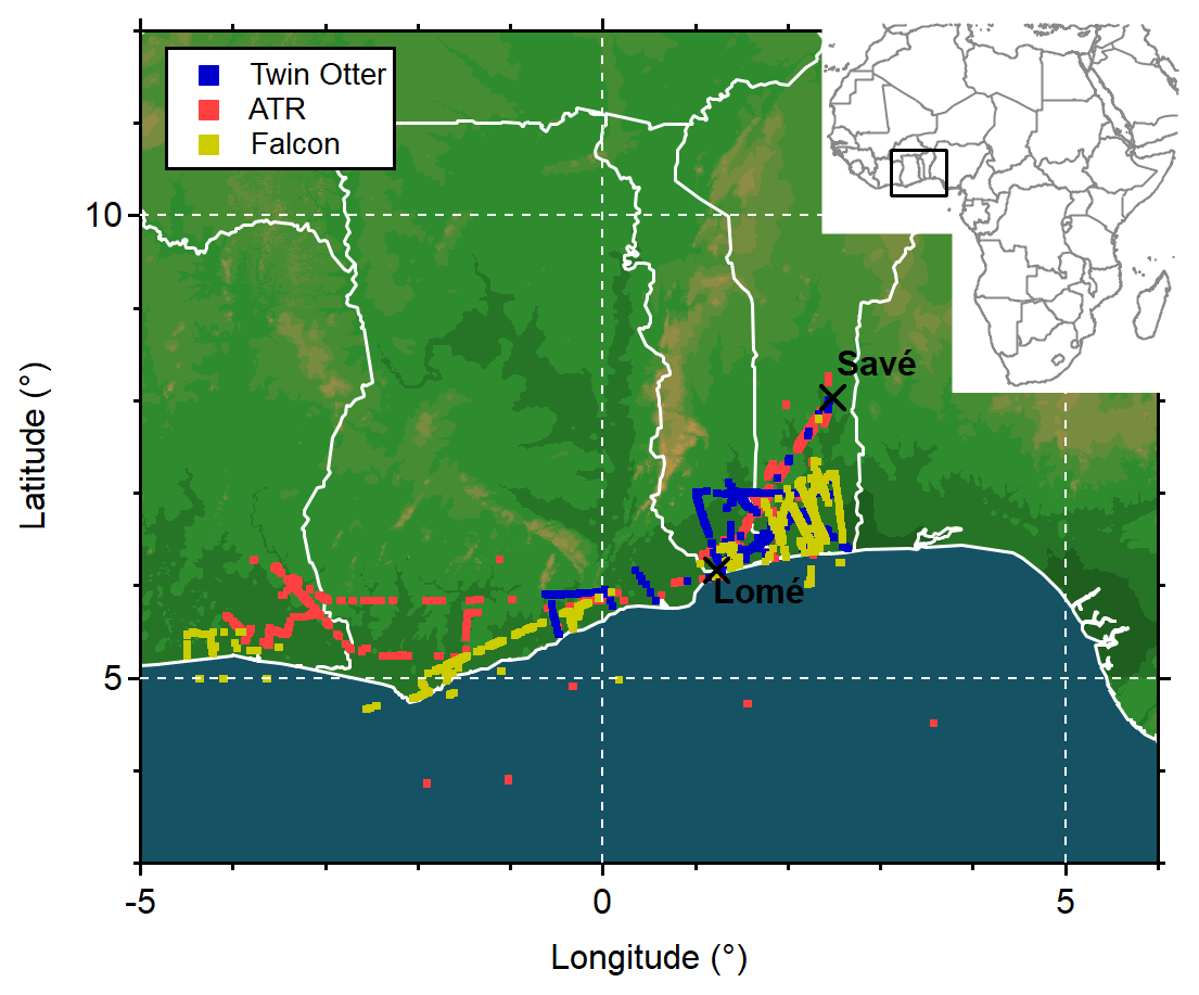
Figure 1 Map showing the parts of the flight trackers where airborne cloud measurements were made below 1 km above mean sea level. The locations of Lomé and Savé are marked as many research flights took place between these two locations.

The large majority of measurements were taken over the African continent. Flights over the sea were carried out on 11 d during the campaign, and these are sufficient to gauge the variability of aerosol offshore. Cloud penetrations on these offshore flights were relatively few, and it is difficult to gauge how statistically robust the offshore cloud measurements were. In this analysis we use cloud data from all flights of the campaign and mostly only consider data from the lowest 1 km to investigate the effects of aerosol on boundary layer clouds over the African continent.

2.1 In situ instrumentation

Each aircraft was equipped with a suite of instrumentation to measure basic meteorological variables such as temperature, humidity, pressure, and winds. Further details are provided by Flamant et al. (2018b). Cloud drops 3–50 µm in diameter were measured using a cloud droplet probe (CDP) on the Twin Otter, CDP and/or fast CDP on the ATR, and a cloud–aerosol spectrometer (CAS) on the Falcon (Baumgardner et al., 2001; Voigt et al., 2017). Both CDPs had modified pinholes to reduce coincidence (Lance, 2012); however, the CAS did not, and the CAS CDNC measurements were corrected for coincidence at high concentrations as described by Kleine et al. (2018). Each instrument had its sample area measured using a droplet gun prior to the campaign, and sizing was calibrated in the field using glass beads of known size and refractive index. To ensure comparability between CDNC measurements on the different platforms, we performed a statistical analysis of all CDNC measurements made between 0 and 100 km inland over Togo/Benin at altitudes below 1 km. CDNC measured on the different platforms showed excellent agreement, with the medians and quartiles all agreeing within 5 %.

We also consider cloud drop effective radius, defined as

$$R_{\mathrm{Eff}}={\displaystyle \frac{{\int }_{\mathrm{0}}^{\mathrm{\infty }}{R}^{\mathrm{3}}n\left(R\right)\mathrm{d}R}{{\int }_{\mathrm{0}}^{\mathrm{\infty }}{R}^{\mathrm{2}}n\left(R\right)\mathrm{d}R}},$$

where n(R) is the number concentration of drops with radius R.

For R_Eff, average vertical profiles between 0 and 100 km inland showed the median values agreed within ∼1 µm, which is within the uncertainties of the instruments, and the interquartile ranges were similar for each platform.

Data were considered in cloud when the measured liquid water content (LWC) was greater than 0.1 g m⁻³. This relatively high LWC threshold minimises the effects of diffuse cloud edges on our measurements and removes swollen aerosol layers (see Deetz et al., 2018a; Haslett et al., 2019a). Measurements of CDNC are reported in number per cubic centimetre (cm⁻³), corrected to standard temperature and pressure (STP, 273.15 K and 1013.25 hPa).

Aerosol composition was measured by compact time-of-flight aerosol mass spectrometers (AMSs, Drewnick et al., 2005). Two AMS instruments were mounted on the ATR and Twin Otter, which were each calibrated using nebulised ammonium nitrate and ammonium sulfate to determine absolute and relative ionisation efficiency. We also consider aerosol size distributions, which were measured using GRIMM optical particle counters (model 1.109 on the ATR and 1.129 on the Twin Otter and Falcon), and a scanning mobility particle sizer (SMPS) on board the ATR. Further details on the AMS and SMPS are provided by Brito et al. (2018) and Haslett et al. (2019b). From the GRIMM measurements we consider only the total concentration of particles larger than 250 nm (N₂₅₀), and from the SMPS we use aerosol size distributions in the range 20–500 nm. The strength of the GRIMM dataset is that all three aircraft had instruments running on every flight, making it a useful dataset for measuring changes in accumulation mode aerosol concentrations. The SMPS data coverage is more limited and is restricted to straight and level runs, but it provides a more detailed measurement of the aerosol size distribution. Aerosol data were screened for cloud using a threshold for LWC of 0.01 g m⁻³ and CDNC of 10 cm⁻³, and data exceeding these thresholds were removed.

Carbon monoxide (CO) concentrations were measured using infrared absorption spectrometry by an Aero-Laser AL5002 on the Twin Otter, SPectromètre InfraRouge In situ Toute altitude (SPIRIT, Catoire et al., 2017) on the Falcon, and a Picarro Analyzer G2401-m on the ATR. We also consider vertical velocity, which was measured using wind probes on the ATR and Falcon.

2.1.1 Cloud satellite measurements

Using satellite measurements allows us to view the cloud field over a large region. We used the optimal cloud analysis (OCA, Watts et al., 2011) product taken from the Meteosat Spinning Enhanced Visible and InfraRed Imager (SEVIRI) spectrometer. This product provides cloud top pressure (CTP) and cloud optical thickness (COT) for the top two cloud layers (looking from above), for scans every 15 min. We use this product to derive the LLC fraction (for pressures above 680 hPa), as described in Appendix A. Comparison with the LLC fraction using ceilometers, based at the DACCIWA supersites near Savé and Kumasi (Kalthoff et al., 2018), showed that this satellite-derived product agreed with ground measurements within ∼10 % absolute cloud fraction, capturing both the absolute values and also the diurnal cycle, particularly during daylight hours. Further details are provided in Appendix A.

2.1.2 Parcel modelling

Parcel model simulations of aerosol activation were carried out using the Aerosol-Cloud and Precipitation Interactions Model (ACPIM) (Connolly et al., 2009). Multiple aerosol modes of defined dry size distribution and composition can be initialised, and the simulated air parcel rises at a prescribed updraft velocity. ACPIM uses bin microphysics and thermodynamics to evaluate the rate of condensation of water in each size bin numerically using the diffusional drop growth equation and Köhler theory (see Topping et al., 2013), so it does not rely on bulk parameterisations of cloud drop activation. The number of particles in each aerosol mode growing above the critical diameter is then evaluated to determine the CDNC.

ACPIM was initialised starting at 95 % humidity, 296 K, and 960 hPa, which are typical of conditions just below cloud base over Togo. Aerosol size distributions from SMPS and relative compositions from AMS were averaged over regions at various distances offshore or inland over SWA, and these were used to initialise the model for several runs at different updraft velocities. The hygroscopicity parameter (κ) values of inorganic and organic aerosols were assumed to be the same as ammonium sulfate and fulvic acid, which is chemically similar to highly aged organic aerosol (Jimenez et al., 2009). By using fixed, representative thermodynamic starting conditions, varying the updraft velocities and aerosol number, size, and composition allows us to determine the relative sensitivities of CDNC to both variables.

Our simple modelling scheme does not include factors such as entrainment, collision–coalescence, or an investigation into the impacts of aerosol mixing state, which can have a large effect on calculated cloud condensation nuclei (CCN) (Ren et al., 2018). We have also only considered a limited number of aerosol species, and other components such as black carbon, sea salt, and mineral dust will have been present. This is not intended to be an exact simulation, but a sensitivity analysis using physically reasonable approximations. A detailed study of aerosol activation is beyond the scope of this analysis and is non-trivial (e.g. Sanchez et al., 2017). Additionally, we have no measurements with which to constrain factors such as the size dependence of chemical composition and mixing state, which strongly affect the accuracy of CCN closure calculations (Moore et al., 2013), so such an investigation would be purely speculative.

3 Results

3.1 Diurnal cycle of low-level cloud cover

Figure 2 shows the average diurnal cycle of LLC fraction over Togo and Benin, where the aircraft operated, plotted versus distance north of the coast and approximate latitude. LLCs peaked around 10:00 LST and fell to a minimum around 18:00 LST. The initial surface warming in the few hours after sunrise causes the nocturnal clouds to rise and thicken, before eventually breaking up (van der Linden et al., 2015; Kalthoff et al., 2018). Cloud cover was generally greater inland than offshore, except for a period in the late afternoon/early evening. A region of more extensive cloud cover was seen developing overnight, around 50–150 km inland. This is the region the maritime inflow reaches on a typical evening, though it is interesting that cloud cover did not increase overnight nearer to the coast. The highest LLC fraction was around 250 km inland, in a region that began to develop overnight but became particularly pronounced during daylight hours. A further region of higher cloud cover was seen just inland of the coast. These are most likely sea breeze clouds developing from mid-morning to the early afternoon and moving up to ∼50 km inland before dissipating. Lower levels of cloud cover (average 0.24) were seen over all inland areas between 16:00 and 00:00 LST. By taking the mean over several weeks we lose the extremes of these values – on some evenings cloud cover was zero and on some mornings it reached 100 %. This averaging allows us to assess which features are statistically robust and minimises transient features in the cloud field. Figure 2 bears a striking similarity to similar diagrams of boundary layer temperature and relative humidity presented by Deetz et al. (2018a), suggesting transport of cool, humid air inland by the maritime inflow is a key factor in determining LLC cover.

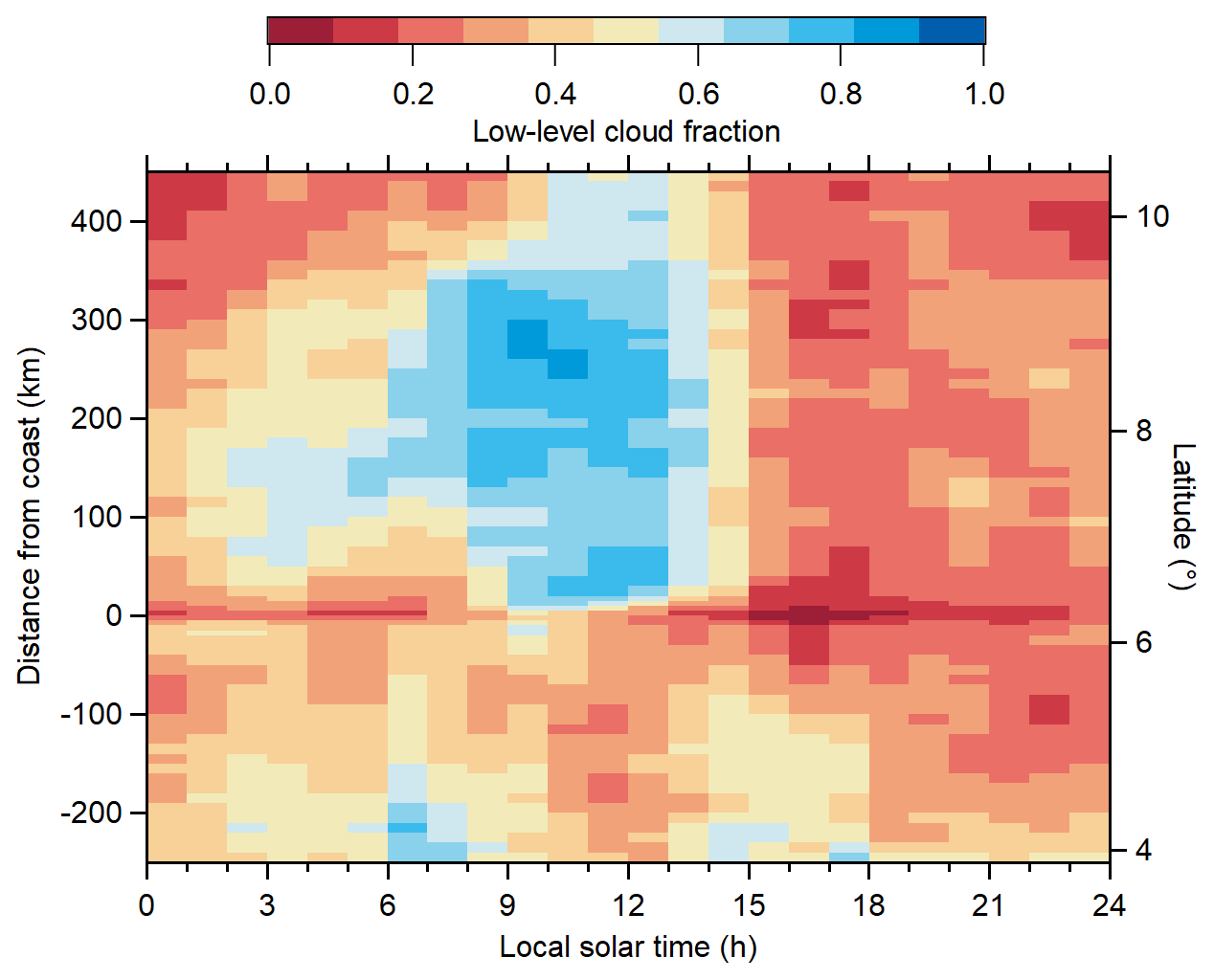
Figure 2 The diurnal cycle of mean low-level cloud fraction at different distances inland or offshore over Togo and Benin (4–11^∘ N, 0.6–2.75^∘ E), taken from the LLC flag derived from SEVIRI cloud data. The data are shown from the time period coinciding with the DACCIWA aircraft campaign: 29 June–16 July 2016. The latitude scale on the right axis is approximate, as the latitude of the coastline varies by 0.6^∘ over Togo and Benin.

3.2 Regional variation in low-level cloud cover

Figure 3 shows the orography of West Africa and a map of LLC fraction at its 10:00 UTC peak. The LLC fraction decreased dramatically in the drier regions north of ∼10–11^∘ N. South of this latitude, the largest LLC fraction was seen on the upwind side of slopes and the lowest on the leeward sides, for a southwesterly monsoon flow. Additionally, a patch of lower LLC fraction is seen just offshore of Ghana, Togo, and Benin, which is related to the colder waters there due to the coastal upwelling system (see Flamant et al., 2018a). The areas of high mean LLCs are the most robust features, with the lowest standard deviation, meaning patches of continuous cloud were present on almost all days during the campaign. Areas with lower average LLC fraction had higher standard deviation and were therefore more variable; the cloud cover in these regions varied day to day but was lower on average. The features in our mean LLC fraction over the region are broadly similar to those presented in multi-year satellite observations by van der Linden et al. (2015), meaning the measurement period is likely to be broadly representative of a typical monsoon season. The absolute values we present are more in line with the synoptic observations than the satellite measurements in the previous work, as the LLC fraction product here takes into account times when LLCs would not be visible due to higher cloud obscuring the view.

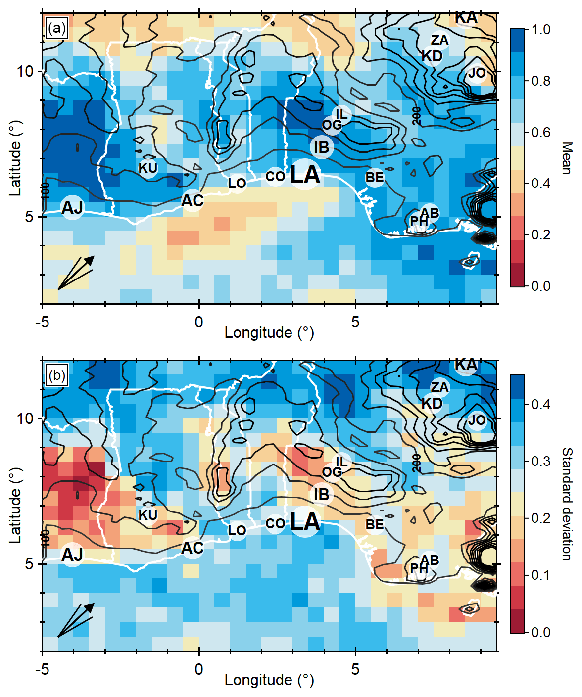
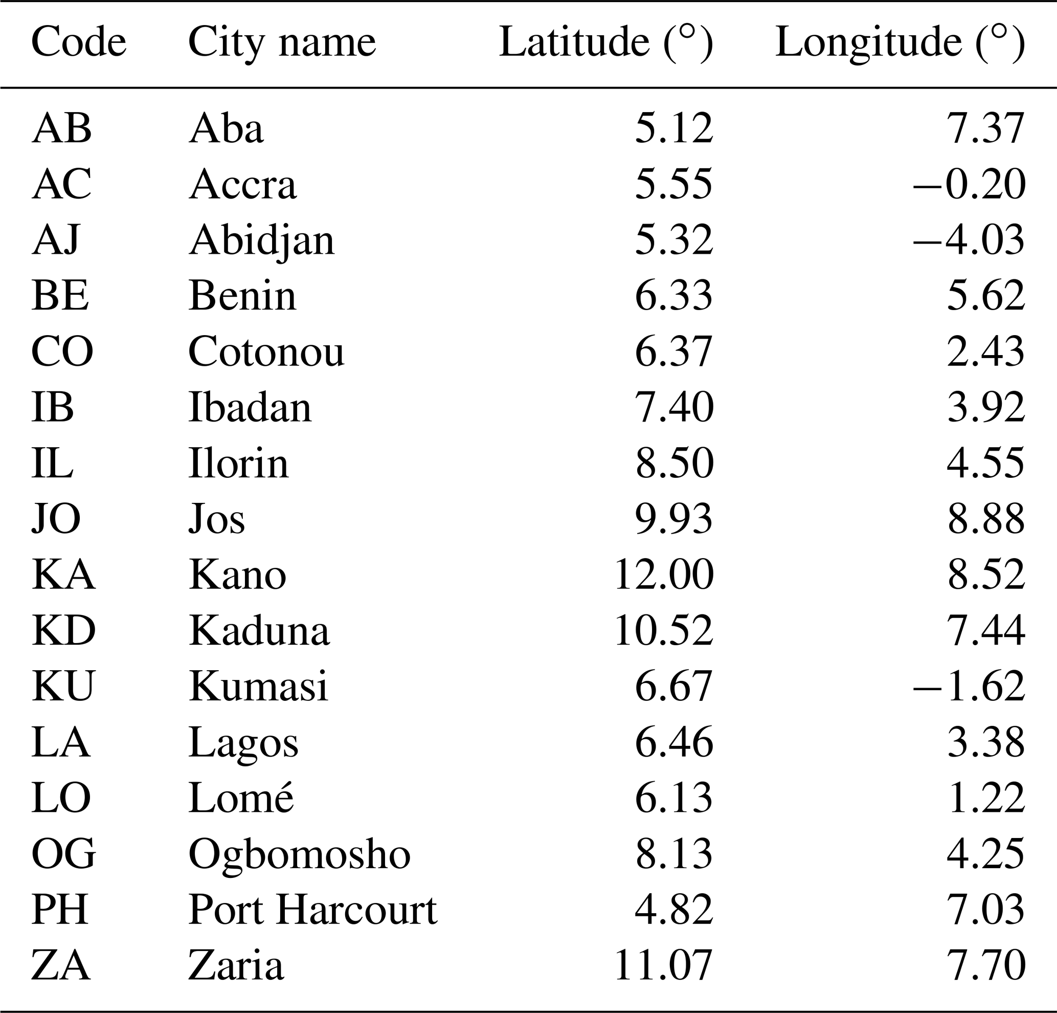
Figure 3 Mean and day-to-day standard deviation of low-level cloud fraction between 10:00 and 11:00 UTC during the DACCIWA aircraft campaign, 29 June–16 July 2016, taken from the LLC flag derived from SEVIRI cloud data. The contours show the elevation of the land surface and are labelled in metres above mean sea level. Text markers show the locations and abbreviated names of large cities in the region, which are listed in Table 1. The text size gives a qualitative indication of the relative population of each city. The arrow markers in the bottom left show the median and quartiles of wind direction, measured inland below 1 km between 10:00 and 11:00 UTC.

Figure 3 also shows the major population centres in the region. Pollution plumes are expected to extend for hundreds of kilometres downwind of the major cities (Deroubaix et al., 2019). Figure 3 does not show any features extending downwind of the major cities that would represent a signature for anthropogenic influence on cloud cover on a regional scale. This was also the case in plots similar to Fig. 3 at all times of day.

Table 1 List of cities in Fig. 3.

3.3 Regional variation in cloud microphysics

To investigate the effect of local emissions on cloud microphysical properties, we collated cloud measurements below 1 km in altitude from all three aircraft and compared them with distance to the coast (and the population centres nearby) on a north–south axis, as shown in Fig. 4a. Figure 4b shows corresponding normalised histograms in the different regions. The limited spatial area of the aircraft sampling means that regional-scale orographic effects discussed in Sect. 3.2 are not likely to have a large effect on in situ cloud properties. The heterogeneous nature of the dataset means that some areas and some days have large numbers of data points recorded, while others have relatively few. In particular, cloud measurements over the sea were sparse compared to inland. To give an indication of how statistically representative our data are, the number of data points and number of individual days the data are from are also listed in Fig. 4a.

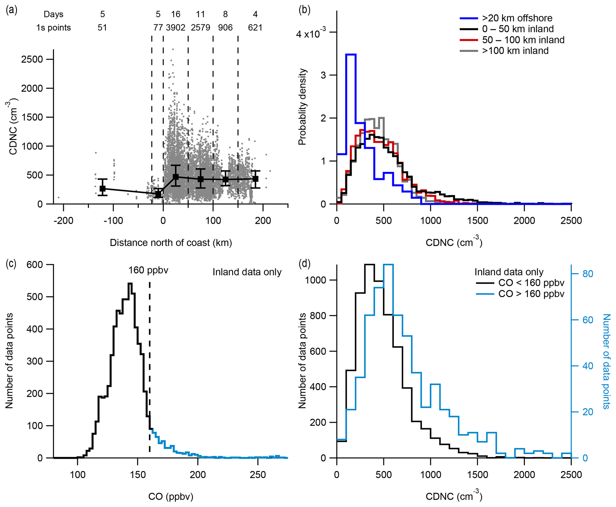
Figure 4 Measured CDNC for all data below 1 km, stratified by distance inland and pollution conditions. Panel (a) shows all data as a function of distance from the coast. The markers and error bars show the median, 25th, and 75th percentiles. The numbers at the top show the number of different days' worth of data in each bin, as well as the number of individual data points. Panel (b) shows normalised histograms of CDNC at different distances from the coast. Panel (c) shows a histogram of in-cloud pollution, and panel (d) shows normalised histograms of inland CDNC stratified by CO concentrations.

Offshore, we split the data up into two bins. The aim of the offshore analysis is to consider clouds and pollution conditions representative of the air upwind of the DACCIWA region, which is then brought inshore by the wind. Close to the coast, several factors may cause terrestrial pollution to be transported to an area offshore. Firstly, some areas of the coast are more prominent than others; for example the area located just offshore near Lomé may be downwind of Accra if the wind was blowing from a west-south-westerly direction. Secondly, sea breeze circulations may act to recirculate pollution (Flamant et al., 2018a). Additionally, a shipping corridor near to the coast presents a local source of CO and aerosol. In Fig. 4a there is no apparent effect of any pollution near to the coast, but plumes of CO and aerosol were observed up to 20 km offshore that would affect the analysis in Sects. 3.6 and 4. For the remainder of this analysis, when considering “offshore” data, we therefore only consider measurement made at least 20 km south of the coast, to unambiguously remove any possibility of local terrestrial emissions affecting our offshore measurements.

In the offshore bin, there were CDNC measurements from five individual days, and the distribution of measured CDNC in Fig. 4b appears bimodal, with a main mode centred around 100–200 cm⁻³ and a smaller mode centred around 500 cm⁻³. Looking at Fig. 4a, this bimodality is the result of sampling different populations of clouds. This may be due to variable pollution conditions offshore or some other factor. Bennartz (2007) studied CDNC in the global marine boundary layers and found that the average CDNC in the pristine South Atlantic was 67 cm⁻³, reported in ambient temperature and pressure. For stratocumulus topping the South Atlantic marine boundary layer at 800 hPa and 280 K, this number is roughly equivalent to 87 cm⁻³ when corrected to STP, which lies around the 10th percentile of the CDNC measured in offshore clouds in the DACCIWA region, meaning the offshore measurements presented here were representative of moderately polluted clouds.

Moving inland, several differences are apparent. The inland CDNC distributions in Fig. 4b are approximately Gaussian, centred around ∼400 cm⁻³, but with long tails extending up to over 1000 cm⁻³, which were measured most frequently near the urban centres near the coast and diminished further inland. Some clouds were observed with CDNC over 1500 cm⁻³. These long tails on the distributions are due to the effect of thick urban plumes, but they only represent a relatively small fraction of the inland data. The large majority of CDNC measurements inland were in the range 200–840 cm⁻³ (10th and 90th percentiles), and medians were 470 cm⁻³ up to 50 km from the coast and ∼430 cm⁻³ further inland. It is possible that some of this small difference in the medians may be due to measurement of more convective sea breeze clouds near the coast, but it is relatively minor overall.

To investigate the effect of local pollution on CDNC, Fig. 4c shows the distribution of CO concentrations measured in inland clouds. The inland CO data show a mode with mean and standard deviation of 141±17 ppbv, but the distribution is asymmetric, with a tail extending to higher values above around 160 ppbv. We therefore used this value of 160 ppbv (the 93rd percentile) as a threshold to distinguish the thickest pollution plumes. Our measurements in this polluted tail were generally in and around the major cities, which were one of the research themes of the DACCIWA campaign. On the regional scale these are likely to be over-represented compared to the more sparsely populated regions of Ghana and Côte d'Ivoire but may be under-represented compared to the more polluted regions of coastal Nigeria. For comparison, the mean and standard deviation of in-cloud offshore CO concentrations were 143±11 ppbv. This offshore value, and similarly the minimum inland CO concentrations of ∼100 ppbv, is significantly enhanced compared to CO concentrations in the unpolluted South Atlantic, which reach lows of 60 ppbv in the absence of transported biomass burning smoke (Zuidema et al., 2018). This contrast highlights the ubiquity of transported biomass burning smoke affecting the DACCIWA region (Haslett et al., 2019b).

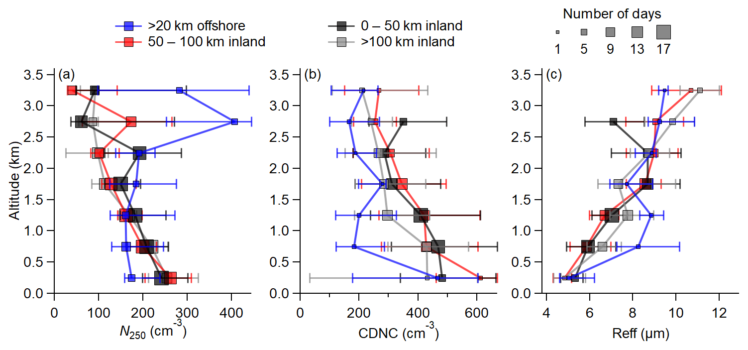
Figure 5 Average vertical profiles of aerosols larger than 250 nm (a), cloud drop number concentration (b), and effective radius. The markers are the medians and are different sizes depending on the number of individual days the data are taken from. The error bars show the 25th and 75th percentiles, and the solid lines connect the medians. The cloud profiles show the average properties of the cloud field, which often contained multiple discreet layers.

Using the 160 ppbv CO threshold to stratify the CDNC highlights the effect of pollution plumes, which we show in Fig. 4d. Using only the inland data here removes any possible bias from differing conditions (for example dynamics) over the sea. The data in Fig. 4d show enhanced CDNC in the polluted plumes, with the entire distribution shifted around 1.5 times higher. However, these highly polluted plumes represent less than 10 % of the inland data measured over the region.

There appeared to be a difference between the offshore and inland clouds that was not related to differing pollution. Inland clouds with CO <160 ppbv (i.e. similar to levels found offshore) had a median CDNC of 430 cm⁻³, compared to 265 cm⁻³ offshore. However, Fig. 4b shows some offshore clouds that had CDNC and CO comparable to those found inland. With the limited offshore data available we are unable to fully quantify whether there was any systematic difference, which might be expected due to different dynamical conditions.

3.4 Vertical profile of cloud microphysics

Figure 5 shows average vertical profiles of N₂₅₀, cloud drop number concentration, and cloud effective radius, measured at different distances north or south of the coast. The aerosol measurement here is only particles larger than 250 nm, so it is representative of the variability of the accumulation mode, though not the total number. N₂₅₀ does not show any variability related to smaller particles. Inland, accumulation mode aerosol concentrations were highest closer to the ground and decreased with altitude up to around 2–2.5 km. There was relatively little meridional variation inland, but aerosol concentrations were enhanced by around ∼40 % near the ground compared to offshore concentrations. This enhancement decreased with altitude, as concentrations offshore were fairly constant up to 2.5 km, and above 2.5 km offshore concentrations were higher than those inland. Together, these aerosol profiles suggest local terrestrial sources adding to the background aerosol on a regional scale. In the boundary layer, the southwesterly winds brought offshore pollution inland, and local city emissions were added to the pollution transported from offshore, but, above the inversion at boundary layer top, the wind shifted to a regime dominated by the African easterly jet and this linkage was broken. Above the boundary layer, distinct biomass burning plumes were encountered more often, which caused the larger variability in N₂₅₀ in the free troposphere.

The CDNC profile inland (Fig. 5b) shows a decrease with altitude, with a similar profile to N₂₅₀, but the relative decrease was lower in magnitude. Inland there was high variability within all regions but little difference between the average values of CDNC, though >100 km inland concentrations were ∼10 % lower than closer to the coast. Offshore concentrations at almost all levels were significantly lower than those inland, and the difference was larger than the differences in aerosol and did not correlate with differences in the aerosol vertical profiles. However, the majority of offshore bins in Fig. 5b show data from one or two individual days, so they may not be representative of offshore clouds in general. If the difference is representative, it does not appear to be directly related to differences in accumulation mode aerosols.

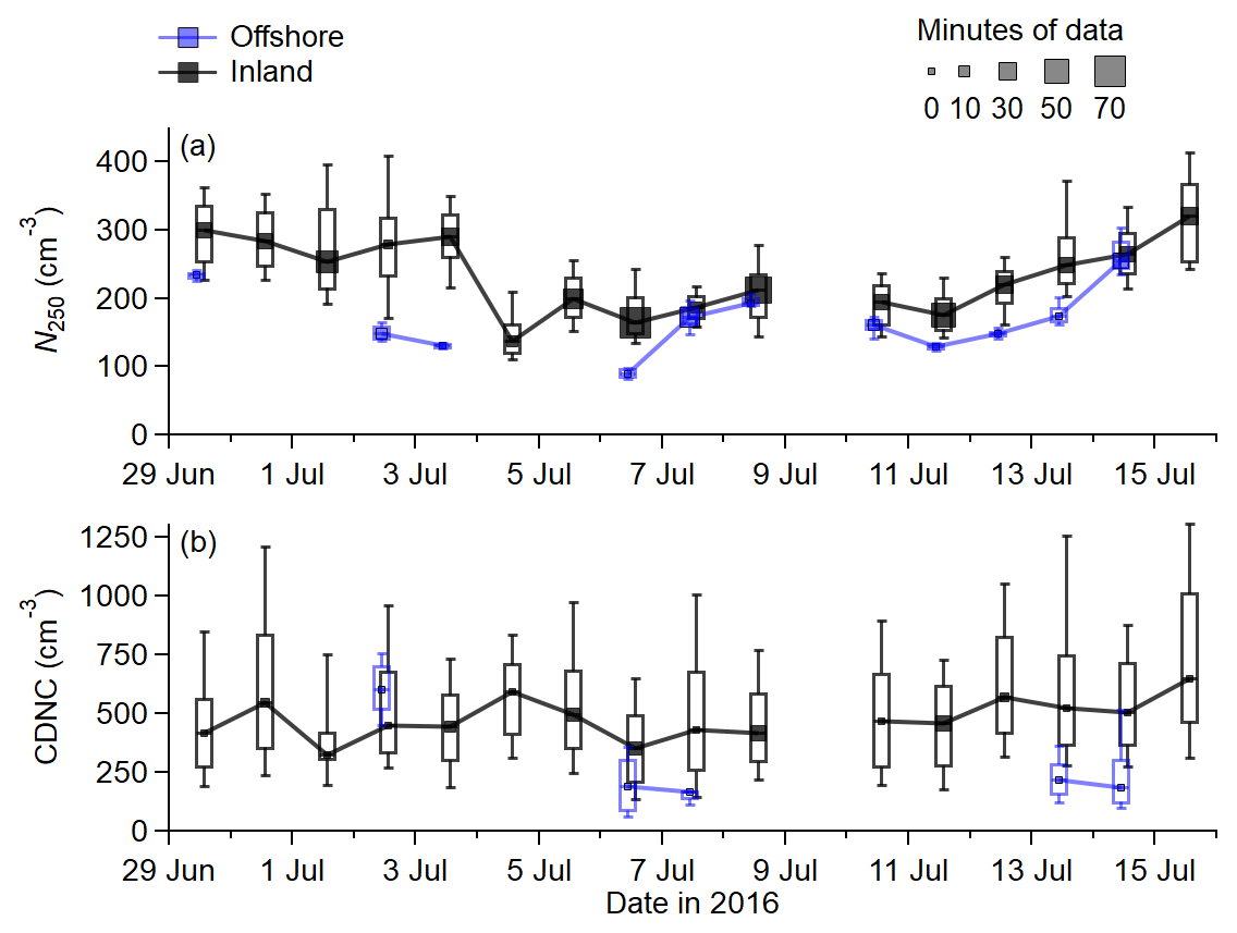
Figure 6 Day-to-day variation in N₂₅₀ (a) and CDNC (b). The data shown are from all data measured below 1km. The markers, boxes, and bars show the medians, 25th and 75th percentiles, and the 10th and 90th percentiles respectively. Offshore data were collected over 20 km south of the coast.

Figure 5c shows the corresponding cloud effective radius profile. Again, there was relatively little difference inland, particularly in the boundary layer, and on the whole R_Eff increased with altitude. In the free troposphere there was more deviation, and R_Eff did not always increase with altitude. This is due to the structure of clouds over SWA; multiple cloud layers with distinct and separate bases were often present, meaning clouds at higher altitudes were not necessarily deeper than those below, and cloud observations at higher altitude were not necessarily higher above the cloud base than observations at lower altitude. Between 0.5 and 1.5 km, the clouds offshore tended to have higher R_Eff than those measured inland at the same altitude, which is consistent with the lower CDNC measured in this altitude range. However, throughout the rest of the lower troposphere, including near the surface, the clouds measured offshore had similar R_Eff to those measured inland at the same altitude, despite generally lower CDNC. This implies that these offshore clouds had lower liquid water contents than inland clouds at the same altitude, suggesting that clouds offshore may have been influenced by a different thermodynamic structure, such as different temperature or humidity profiles causing different cloud base heights.

Overall, relatively little systematic spatial variability was seen inland in aerosol or cloud parameters. There are differences in aerosol and CDNC between inland and offshore clouds, but not in R_Eff, meaning the differences cannot be solely due to increased aerosol activation inland. For the remainder of this analysis we will consider only clouds measured in the lowest kilometre of the atmosphere, as this covers the majority of the cloud measurements made in the morning, and to minimise the influence of the African easterly jet. Although the properties of individual clouds were variable, the average inland clouds below 1 km were fairly homogeneous regardless of the distance inland, meaning we can consider all inland clouds together and develop better statistics of the day-to-day variability and diurnal cycle of cloud properties.

3.5 Day-to-day variability

In the previous sections, we demonstrated that the ubiquitous background aerosol reaching SWA caused all clouds to be fairly polluted. Figure 6 shows the day-to-day variability in both the offshore and inland aerosol concentrations, as well as the CDNC. For the accumulation mode aerosol, the inland concentrations of N₂₅₀ were around 40 % higher than offshore, though there was some day-to-day variability in this ratio. The average inland enhancement is in excellent agreement with Haslett et al. (2019b), who also found a 40 % enhancement in accumulation mode aerosol in continental background areas compared to upwind marine, using SMPS measurements averaged over the whole campaign. The day-to-day averages of the accumulation mode aerosol number concentration from the SMPS showed good correlation with the GRIMM, with R²=0.7, but data were only available for 9 d inland and 2 d offshore. The GRIMM data therefore show a similar trend to the SMPS, but with greater coverage. The mean and standard deviations in daily N₂₅₀ are 170±50 cm⁻³ offshore and 230±50 cm⁻³ inland, meaning the average variabilities were similar. Together with the good correlation, this suggests that aerosol imported from offshore had a strong influence on the average amount, and day-to-day variability, of accumulation mode aerosol inland.

The day-to-day variability in the aerosol was not strongly represented in the CDNC measurements in Fig. 6b. There was a degree of correlation in the median CDNC and N₂₅₀ measurements (R²=0.72) after the 5th of July, but there was no correlation in the first half of the campaign. On a cloud-to-cloud basis this correlation was dwarfed by the inherent local variability in CDNC. Comparing the inland CDNC to offshore, on four days the median values inland were 85–175 % higher than those measured offshore but 25 % lower on one day. These differences were not correlated with differences in the offshore and inland aerosol. As was stated in Sect. 3.3, we do not have sufficient measurements to investigate or explain these differences in detail, or to assess if they are representative. On any individual day, the CDNC measurements were much more variable than the aerosol concentrations, suggesting highly localised factors such as entrainment or dynamics may have had an influence on the CDNC. Overall, the day-to-day variabilities in the inland CDNC and N₂₅₀ were both ∼20 %, and there was a degree of correlation for some of the project, suggesting aerosol concentrations may have had some effect on daily CDNC. In the next section, we discuss diurnal variation to investigate these factors in more detail.

3.6 Diurnal variability of aerosols, clouds, and dynamics

The variation in inland CDNC at different times of day is shown in Fig. 7a. As some of the measurements were taken over a wide range of longitude, here we used the local solar time (LST) instead of UTC. A trend is apparent in the data, as CDNC increased inland throughout the morning and remained higher through the afternoon. The inland CDNC measurements were 45 %–60 % higher in the afternoon than before 08:00. The median of all CDNC measured inland in the morning was 430 and 540 cm⁻³ in the afternoon. We draw this distinction because cloud cover peaked in the late morning, before decreasing in the afternoons as the clouds broke up. The 90th percentiles of CDNC in Fig. 7a exhibited a more dramatic increase in the afternoon, indicating a greater cloud drop concentration in the more convective broken clouds.

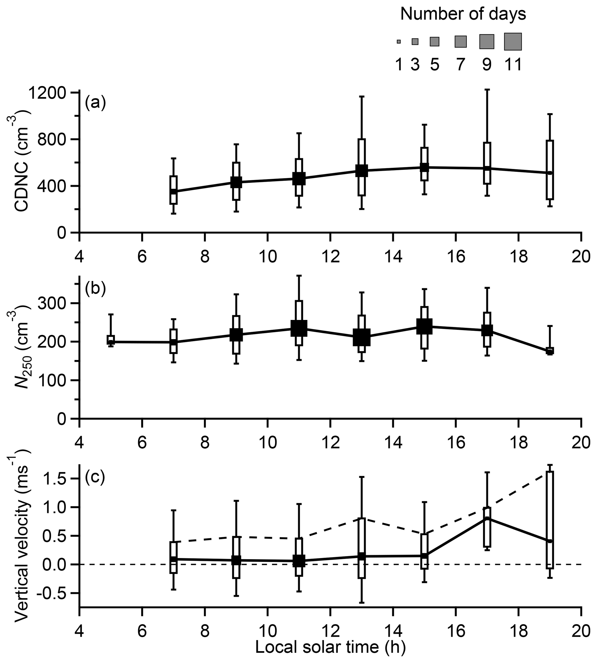
Figure 7 Inland diurnal variation in CDNC (a), N₂₅₀ (b), and in-cloud vertical velocity (c). The data shown are from all data measured below 1 km. The markers are the medians and are different sizes depending on how many individual days the data are taken from. The boxes are the 25th and 75th percentiles, and the bars are the 10th and 90th percentiles. The solid lines connect the medians, and the dashed line in panel (c) connects the 75th percentiles.

CDNC is determined by the supersaturation in an updraft and the concentration of aerosols that activate at that supersaturation. Figure 7b and c show the diurnal variations in N₂₅₀ and in-cloud vertical velocity. The accumulation mode aerosol showed no strong diurnal variation, varying only ±10 % during the day. In comparison, the distributions of vertical velocity showed a shift towards stronger updrafts in the afternoon. In any stable cloud layer the median vertical velocity is zero, and this was the case for all times of day shown in Fig. 7c other than the few cloud measurements made after 16:00 LST. As the median value of vertical velocity in a stable cloud is zero, the 75th percentile can be considered a representative updraft and is useful to investigate changes in updrafts that are present at cloud base, where the majority of aerosol activation occurs. Vertical velocity does not vary strongly with altitude in stratocumulus clouds (Wood, 2012), so although our measurements are not just from cloud base, they are still suitable to use in our simulations.

The distribution of vertical velocity was fairly stable throughout the morning, with 75th percentiles around 0.45 m s⁻¹ and 90th percentiles around 1 m s⁻¹. In the afternoon, the clouds became more convective, with 75th percentiles of vertical velocity of 0.5–1.6 m s⁻¹ and 90th percentiles of 1.1–1.7 m s⁻¹. The stronger updrafts in the afternoon suggest that dynamics played a role in the diurnal cycle of CDNC but cannot fully explain the changes. In the next section we use parcel model simulations to quantify the effect of these factors on CDNC.

4 Parcel model simulations

The limited offshore dataset and the possibility of differing dynamics inland makes it difficult to assess the impact of local aerosol emissions on cloud properties based on measurements alone. To further investigate the relative sensitivities of CDNC to aerosol properties and updraft velocities, we conducted a series of parcel model simulations using ACPIM, described in Sect. 2.1.2. We initialised the model with representative thermodynamic conditions and varied the updraft velocity and aerosol size distribution and composition based on the measurements made in the field campaign.

Figure 8 Aerosol size distributions (a–c) and accumulation mode composition measurements (d–f) made over SWA that were used as input into ACPIM. The averaged local emissions were calculated by subtracting the offshore transported aerosol from the inland regional aerosol.

4.1 Aerosol size and composition

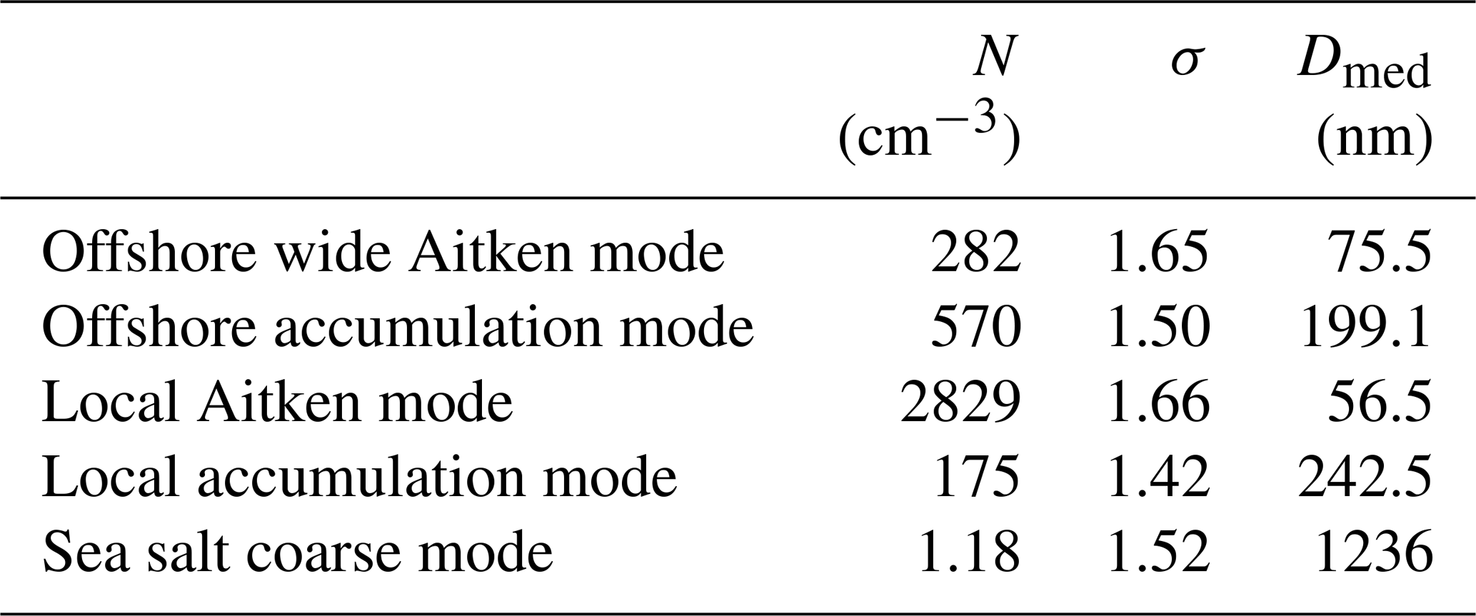
The average measured aerosol size distributions are shown in Fig. 8a–c. Here, the data coverage was more limited, and the scanning time of the instrument was 90 s, so we used a simple mean of all the data inland or offshore, averaging out any diurnal or day-to-day variation. While the Aitken mode was variable inland due to highly localised anthropogenic emissions, the accumulation mode showed minimal variability as a significant fraction of particles in this size range were due to long-range transport (Haslett et al., 2019b). This averaging approach is therefore reasonable to inform cloud activation modelling, as the accumulation mode is the source of CCN. The average measured offshore aerosol size distribution and accumulation mode composition are shown in Fig. 8a and d. Two lognormal fits were used to approximate this size distribution for use in ACPIM. The average measured inland aerosol size distribution and accumulation mode composition are shown in Fig. 8c and f. The offshore size distribution was subtracted from the inland distribution to give an estimate of the average contribution of dispersed local emissions to regionally averaged inland aerosol over SWA. Two lognormal fits were then used to approximate the average local emissions, and the sum of the four fitted modes makes up the measured size distribution inland. The lognormal fit parameters are listed in Table 2. The utility of this approach is that it allows us to scale the transported background aerosol (i.e. the offshore fits) and the local aerosol separately.

Table 2 Lognormal fit parameters for the fits shown in Fig. 8, using the equation $\mathrm{d}N/\mathrm{d}\ln D_{\mathrm{p}}=\frac{N}{\sqrt{\mathrm{2}\mathit{\pi }}\ln \left(\mathit{\sigma }\right)}\exp \left(-\frac{{\left(\ln \left(D_{\mathrm{p}}\right)-\ln \left(D_{\mathrm{med}}\right)\right)}^{\mathrm{2}}}{\mathrm{2}\ln (\mathit{\sigma }{)}^{\mathrm{2}}}\right)$.

The measured size distributions in Fig. 8a and c, and the measured compositions in Fig. 8d and f, are almost identical to similar estimates presented by Haslett et al. (2019b). The difference in our approach when highlighting the impact of local emissions is that we have subtracted the transported background to isolate the effect of dispersed local emissions on regional inland aerosol, whereas Haslett et al. (2019b) measured aerosol in the thickest urban plumes but still on top of the transported background.

The offshore aerosol size and composition are consistent with being a mixture of aged biomass burning (Rissler et al., 2006; Capes et al., 2008; Sakamoto et al., 2015) and Atlantic marine aerosol (Zorn et al., 2008; Taylor et al., 2016). The two modes of local aerosol were an Aitken mode containing the majority of the particle number concentration and a smaller accumulation mode. We are unable to determine the specific source of each mode, but local emissions are largely from domestic wood burning and transport, and when combined these sources are capable of producing aerosols with this size distribution and composition (Maricq et al., 2000; Capes et al., 2008; Vakkari et al., 2014). More informative studies of aerosol size distribution in African cities appear to be absent from the literature. The local Aitken mode, which accounts for the majority of particle number inland, contains particles that were too small to make a significant contribution to CCN in stratocumulus clouds, and the majority of the aerosols that are large enough to activate into cloud drops were still the result of long-range transport.

4.2 Model results

We used the aerosol size distributions and composition shown in Fig. 8 and Table 2 as input for ACPIM simulations at varying updraft velocities. The resultant simulated CDNCs are shown in Fig. 9a. For weak updrafts the different input aerosols make little difference to the CDNC values, as particle activation starts from the largest sizes, where the inland and offshore size distributions were most similar. The difference between the two then increases with updraft velocity. For the representative morning updraft of 0.45 m s⁻¹ (calculated as the 75th percentile of vertical velocity), the calculated enhancement in inland CDNC due to local aerosols is 44 %. This enhancement is larger for stronger updrafts; for the representative afternoon updraft of 0.78 m s⁻¹, it rises to 65 %. In polluted clouds with relatively gentle convection, CDNC is more sensitive to changes in updraft than in aerosol (Reutter et al., 2009). However, Fig. 9a suggests the clouds over SWA are only in this regime for the lowest updrafts, and for the average updrafts the clouds are in a regime where they are sensitive to both changes in updraft and aerosol.

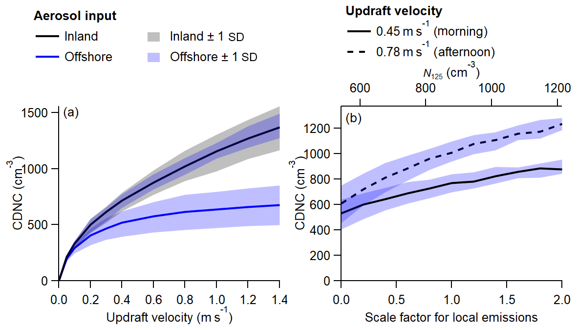
Figure 9 CDNC calculated during ACPIM parcel model runs initialised using measured aerosol size distributions and compositions shown in Fig. 8 and Table 2. The shaded regions show the expected day-to-day variability in CDNC as a result of variation in the aerosol concentrations, based on the standard deviation of measurements shown in Fig. 6a. Panel (a) shows the sensitivity of CDNC to updraft velocities and panel (b) the sensitivity to different scale factors for local emissions in the aerosol input. The smaller and larger updraft velocities in panel (b) are representative of morning and afternoon.

A large fraction of the day-to-day variability expected in the mean inland CDNC, shown by the shadings in Fig. 9, derives from day-to-day variability in the offshore aerosol brought inland. At higher updrafts, the variability from offshore aerosol causes 50 % of this inland variability, but at lower updrafts this fraction increases to 100 %. Using the average morning and afternoon updrafts (as defined above), the modelled CDNC is 31 % higher in the afternoon than in the morning, which compares well to a 26 % increase in the measured CDNC shown in Fig. 7.

Figure 9b shows the effect of varying the local emissions on the calculated CDNCs, using these average morning and afternoon updrafts. For comparison, the top axis in Fig. 9b shows the number concentration of aerosols larger than 125 nm (N₁₂₅) in the input size distributions, as a way of comparing the effects that scaling local emissions have on aerosol concentrations (i.e. transported background plus local emissions). The diameter of 125 nm was chosen as N₁₂₅ is roughly comparable to the modelled values of CDNC in Fig. 9b and is therefore an approximation of the modelled critical diameter, although the actual critical diameter will have been different in each model run and varies as the aerosol size distributions and number concentrations change.

An alternative way of looking at the impact of transported aerosols inland is to say that if local emissions were doubled, N₁₂₅ would only be 38 % higher, and CDNC would only increase by 17 % in the morning and 22 % in the afternoon. If local emissions were halved, N₁₂₅ would be reduced by 19 %, and CDNC would decrease by 13 % in the morning and 16 % in the afternoon. If local emissions were removed entirely, N₁₂₅ would decrease by 38 %, and CDNC would drop by 31 % in the morning and 39 % in the afternoon. Large changes in local emissions cause smaller changes in CDNC because the high aerosol background means they form only a fraction of the total aerosol. Additionally, the local emissions are smaller and less hygroscopic than the background aerosol, so they are less likely to activate. The effect of varying local aerosol emissions does not produce a linear relationship between CDNC and total aerosol concentrations. In particular, the effect of increasing total aerosol concentrations has less of an impact on CDNC than decreasing aerosol. The exact comparability between the aerosol metric and CDNC will depend on the size assumed to be representative of the critical diameter (125 nm in this comparison but would vary as the aerosol changes), but the nonlinearity of the relationship between aerosol and CDNC is independent of this choice of size. This nonlinearity may be related to a reduction in supersaturation for a given updraft velocity, as CCN number concentration increases and water vapour condenses more quickly.

The values of CDNC produced by ACPIM are higher than the median values shown in the ambient measurements. We have acknowledged the limitations of our simplistic approach above, such as the assumptions regarding aerosol mixing state and the lack of entrainment in the model. Moore et al. (2013) summarised 36 previous studies of CCN closure and similarly found that CCN concentrations were generally overpredicted, other than when using size-resolved measurements of aerosol composition. Additionally, a previous comparison by Simpson et al. (2014) showed that ACPIM calculated higher CDNC compared to simpler parameterisations when using multiple aerosol modes. The values of modelled CDNC using the representative morning and afternoon updrafts are between the 75th and 90th percentiles of measured CDNC shown in Fig. 7a, meaning the difference between the average model and measured values is smaller than the variability in the measured data. ACPIM is an idealised simulation and we have used it here primarily to explore the sensitivity to local aerosol emissions rather than arbitrarily try to tune factors such as aerosol mixing state, more realistic dynamics, or entrainment (of which we have limited or no measurements) to make the CDNC agree perfectly.

We performed some additional simulations to explore some possible sensitivities in our assumptions. Firstly we considered the presence of a coarse sea salt aerosol mode, which we isolated from the GRIMM size distributions. The size distribution of this mode is listed in Table 2, and the composition was assumed to be NaCl. As the concentration in the sea salt mode is so low compared to the accumulation mode, this addition of a coarse sea salt mode made less than a 1 % difference to the derived CDNC. We also performed some illustrative runs on the inland aerosol – one possible scenario is that the local Aitken mode aerosols were from primary combustion. We assumed them to be 100 % organic and proportioned the composition of the local accumulation mode to match the total measured organic/inorganic ratio. Compared to the base case, this increased the inorganic fraction in the local accumulation mode from 31 % to 41 %, and the resultant CDNCs showed around a 12 % increase. These simulations show that there are some differences that are attributable to assumptions in aerosol composition and mixing state, but they are likely to be smaller than the differences we show related to the total amount of aerosol and updraft velocity.

5 Discussion

Most stratocumulus clouds are over the oceans, and most previous studies of cloud–aerosol interactions in stratocumulus clouds have focused on clouds in this setting. Allen et al. (2011) observed cloud drop number concentration in the southeast Pacific decreasing from 300 cm⁻³ near the coast to ∼100 cm⁻³ 150 km downwind offshore. Their situation is simpler to visualise as the anthropogenic source regions are well defined, the ocean surface is flat (compared to the land surface), and there is no strong diurnal cycle in ocean surface temperature. In southern West Africa, the situation is made more complex by the combination of local sources and the variability of the dynamics, both in terms of the diurnal cycle and the difference between offshore and inland.

In very remote regions of the South Atlantic, like in the southeast Pacific, clouds are generally clean, with average cloud drop number concentration estimated at 67 cm⁻³ (or 87 cm⁻³ when corrected to STP) (Bennartz, 2007), and effective radius may be ∼15–20 µm for clouds up to 1.5 km in height (Painemal et al., 2014). In this regime, cloud albedo is strongly susceptible to changes in aerosol concentration. In DACCIWA, the limited measurements of offshore clouds were split into one day with CDNC around 300–700 cm⁻³, which was ∼35 % higher than the corresponding inland measurements; and four days with CDNC around 100–200 cm⁻³, 45 %–65 % lower than inland. None of the offshore measurements were representative of clean clouds; offshore clouds were universally more polluted, with higher CDNC and lower R_Eff, than those in the clean regions of the South Atlantic. The ubiquitous presence of aged biomass burning smoke transported from fires in western Central Africa towards SWA provides a source of CCN in greater concentrations than may be found in clean, remote regions.

One of the aims of this paper was to assess the relative impacts of local and transported aerosols on the microphysics of continental clouds over SWA. None of the offshore differences in CDNC, either in the different offshore CDNC on different days or the different offshore/inland ratios, corresponded with differences in the measured aerosol concentrations. Therefore other factors must have been at play to cause the variability in the offshore cloud measurements, such as different dynamics, thermodynamics, or simply random biases due to our limited set of observations. Our measurements of offshore clouds were sporadic rather than systematic, and it is difficult to assess the statistical significance of the variability within these offshore clouds or the differences observed between the clouds measured offshore and inland. Figure 2 shows that, in our measurement region, the low-level cloud fraction offshore was much lower than inland, and most of the inland cloud formed over the continent, rather than forming offshore before moving inland. The complex dynamic and thermodynamic structure of the marine and continental boundary layers (Wood, 2012) and the diurnal cycle of these differences mean that the offshore and inland clouds are not directly comparable to assess the impact of local aerosol emissions.

In contrast, the offshore aerosol measurements are much more robust. There were aerosol measurements from a larger number of days, with a much longer sampling time on each day, and aerosol concentrations are much less susceptible to changes in boundary layer thermodynamics compared to clouds. Our measurements showed an average ∼40 % increase in regional accumulation mode aerosol inland compared to offshore. The accumulation mode is the most important for CCN, as particles smaller than this are too small to activate. Haslett et al. (2019b) also found a 40 % enhancement in the inland accumulation mode aerosol concentrations compared to offshore using SMPS data, which is in excellent agreement with our GRIMM measurements of N₂₅₀. In localised city plumes, highly concentrated emissions had a noticeable increase in CDNC, but these concentrated plumes were not widely observed over the regional scale.

Our model simulations allow us to isolate the effects of specific aerosol modes and dynamics. The increase in CDNC inland due to local aerosols is strongly sensitive to the updraft velocity used in the simulation, but for our representative morning and afternoon updrafts the local aerosols increased inland CDNC by and 44 % and 65 %. As these numbers are larger than our measured increase in accumulation mode aerosol, some of the particles in the Aitken mode fits must be having an influence. Regardless, local aerosols constitute less than half of the regional CCN over SWA. Any future increases in the local anthropogenic emissions during the summer monsoon will be on top of the transported background, and this reduces the sensitivity of CDNC to local emissions, which form less of the total aerosol.

Across the whole of SWA, anthropogenic emissions are dominated by Nigeria, which contains over half of the region's population (United Nations, 2017). The Niger delta is also a large source of industrial pollution. In the boundary layer, Nigeria was downwind of our in situ measurements, so we have no measurements of Nigerian pollution. Under such conditions, Flamant et al. (2018a) and Deroubaix et al. (2019) have shown that Lagos did not influence the air quality to the west (i.e. Benin and Togo). It is possible that local emissions have more of an effect on CDNC in Nigeria, but the baseline CDNC is still likely to have been high enough that this will have a reduced effect on cloud albedo compared to a clean background. Based on the satellite data there was no obvious effect on LLC fraction downwind of Lagos and the Niger delta, suggesting geographical variations in cloud formation and lifetime were still largely controlled by dynamics, orography, and the transport of cool, humid air inland by the maritime inflow.

Over the next few decades, the populations of coastal cities such as Accra, Lomé, and Cotonou are expected to rise dramatically, as are their respective emissions. While this may mean there is more of an effect from local pollution on the cloud field, our results suggest the dominating factors for cloud radiative properties during the summer West African monsoon are likely to remain the transport of biomass burning aerosol from the Southern Hemisphere. Indeed, as the population of western Central Africa is also expected to rise at a similar rate to SWA (United Nations, 2017), increasing rates of agricultural burning may cause this background to rise. In this study we have focused on cloud–aerosol interactions leading to the indirect effects and have not attempted to investigate possible changes to the cloud field by the semi-direct effect or direct effect via changing dynamics, as suggested by Deetz et al. (2018b) and Kniffka et al. (2019). It is vital that future studies examining these effects take into account the transport of biomass burning emissions to SWA from the Southern Hemisphere.

6 Conclusions

This study has assessed factors affecting properties of low-level clouds over southern West Africa during the West African summer monsoon, using an approach combining satellite observations with in situ measurements from the novel DACCIWA dataset. Satellite observations of low-level cloud (LLC) cover suggested regional variation in the cloud field was determined largely by the local orography and transport of cool, humid air inland by the maritime inflow, and no obvious impact of was observed in the large-scale cloud field downwind of major population centres. An assessment of cloud drop number concentration (CDNC) based on aircraft data acquired during the DACCIWA field campaign, as well as parcel modelling, showed that local emissions had a reduced effect on CDNC on the regional scale, as biomass burning pollution transported from the Southern Hemisphere dominated regional aerosol concentrations (Haslett et al., 2019b). This transported pollution also caused a high baseline CDNC inland, putting the clouds in a regime where they had a reduced susceptibility to any further increases in aerosol, and also minimising the impact any enhancements in CDNC are likely to have on cloud radiative effects and precipitation.

We investigated statistics of CDNC on different days, at different times of day, and at different distances downwind of the coast (and the populated regions nearby), to assess the causes of the observed variability. Overall, the large majority of CDNC measurements fell into the range 200–840 cm⁻³, and relatively little meridional variation was seen inland. The day-to-day variability of CDNC showed some correlation with measured aerosol concentrations, but this was not seen across the whole of the campaign. A diurnal cycle was observed, and CDNC increased by 45 %–60 % as clouds began to break up and become more convective in the afternoons compared to measurements made in the early morning. A systematic increase in CDNC was observed in CO plumes near the coastal cities, reaching over 1500 cm⁻³ in some cases. However, these plumes represented only a small fraction of the data measured across the region, and are unlikely to be the major factor determining CDNC inland. Offshore, the limited measurements of CDNC were split into clouds with around 100–200 cm⁻³ and those with around 300–700 cm⁻³. However, relatively few cloud penetrations were made offshore, so it is difficult to assess whether any differences between offshore and inland clouds are statistically representative. In no region, and at no time of day, were clouds observed that were representative of those found in pristine environments, and our measurements were all affected by the ubiquitous biomass burning pollution transported to the region from offshore.

In order to assess the impacts of local urban emissions and transported background pollution on cloud properties, we performed a sensitivity analysis with a parcel model that was initialised with representative aerosol size distribution and composition, as well as thermodynamic conditions based on the ambient measurements. We divided up the aerosol into different modes representing either transported pollution or local emissions and scaled the local emissions to see the effect on CDNC. Doubling local emissions increased the calculated CDNC by 17 %–22 %, whereas CDNC was reduced by 13 %–16 % if local emissions were halved or by 31 %–39 % if they were removed altogether. The aerosol background from transported smoke means local emissions only make up a fraction of total aerosol. Our results suggest that increasing local emissions over the next few decades will therefore have a reduced impact on CDNC.

Compared to clean conditions, this polluted regime means local emissions have a reduced effect on aerosol concentrations, enhanced aerosols have a reduced effect on CDNC, and enhanced CDNC has a reduced effect on cloud radiative properties. As the Southern Hemisphere biomass burning season and West African monsoon coincide every year, and the cloud field during DACCIWA was similar to a previous multi-year assessment by van der Linden et al. (2015), it is reasonable to assume that our observations are typical of clouds over SWA at this time of year. As the population of SWA grows in the coming decades, the transported biomass burning pollution will have a dampening effect on the impacts that growing aerosol emissions have on low-level clouds via cloud–aerosol interactions. Future studies investigating other mechanisms by which aerosols may affect the cloud field, such as by changing atmospheric dynamics and thermodynamics, must take into account the transport of biomass burning smoke from the Southern Hemisphere to SWA.

Appendix A: Low-level cloud flag derivation

The SEVIRI optimal cloud analysis (OCA) product is based on the scheme described by Watts et al. (2011). Cloud top pressure (CTP), cloud optical thickness (COT), and cloud-top effective radius, and their respective uncertainties, are reported every 15 min with a spatial resolution of around 3 km in the DACCIWA region. Here we utilise the CTP for the upper and second cloud layers (CTP₁ and CTP₂) and the COT of the upper layer (COT₁).

Our scheme for determining LLC cover is shown in Fig A1. Pixels are defined as LLCs if either CTP₁ or CTP₂ are statistically significantly above a threshold pressure (CTP_T). Where the greater of CTP₁ and CTP₂ is within the uncertainties of this threshold, the pixel is defined as “borderline” LLCs. Additionally, where the top layer of cloud is not at low level, a threshold COT (COT_T) is used to account for the fact that this thick top layer makes it difficult to detect any other cloud layers below. This extra factor may be responsible for the better agreement between our scheme and ground measurements compared to others (e.g. van der Linden et al., 2015). We chose a value of CTP_T of 680 hPa (∼3.5 km) because the OCA algorithm can sometimes place a cloud on the wrong side of an inversion. 680 hPa is near a minimum in relative humidity (Kalthoff et al., 2018), at a level above the inversion at boundary layer top but below any mid-level clouds.

A comparison to LLC fraction derived from ground-based ceilometers in Kumasi and Savé is shown in Fig. A2. The ceilometers made ground-up measurements of cloud base, compared to top-down satellite measurements of cloud top, which may cause a small uncertainty in the comparison that is difficult to quantify. Surprisingly, the best agreement was generated by ignoring the per-pixel uncertainty in the SEVIRI data (i.e. assuming all values of CTP were absolutely accurate). This comparison showed agreement in the diurnal cycle and absolute values within 10 % LLC fraction, as well as similar levels of variability (i.e. the standard deviations). The comparison was better during the day than at night, in agreement with a similar observations by van der Linden et al. (2015), though using a different LLC scheme.

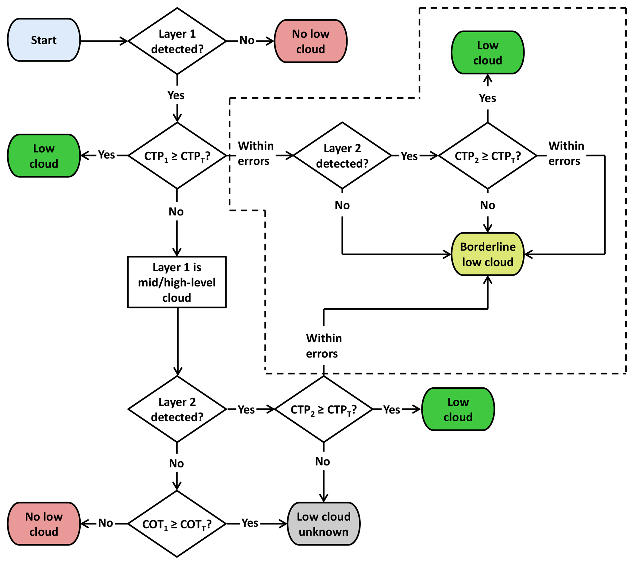
Figure A1 Schematic describing the derivation of the LLC flag from SEVIRI OCA data. We used values of CTP_T=680 hPa and log ₁₀(COT_T)=0. The dashed lines separate off the section of the scheme that is only necessary where the per-pixel uncertainty is considered.

Figure A2 Comparison of LLC fraction derived from satellite and ground-based ceilometer measurements from Savé (a) and Kumasi (b). The satellite measurements were calculated from a 4 pixel × 4 pixel grid centred on the ground site.