Characteristics of atmospheric mercury in a suburban area of east China: sources, formation mechanisms, and regional transport

Speciated atmospheric mercury including gaseous elemental mercury (GEM), gaseous oxidized mercury (GOM), and particulate-bound mercury (PBM) were measured continuously for a 1-year period at a suburban site, representing a regional transport intersection zone, in east China. Annual mean concentrations of GEM, PBM, and GOM reached 2.77 ng m⁻³, 60.8 pg m⁻³, and 82.1 pg m⁻³, respectively. GEM concentrations were elevated in all the seasons except autumn. High mercury concentrations were related to winds from the south, southwest, and north of the measurement site. Combining analysis results from using various source apportionment methods, it was found that GEM concentration was higher when quasi-local sources dominated over long-range transport. Six source factors belonging to the anthropogenic sources of GEM were identified, including the common sectors previously identified (industrial and biomass burning, coal combustion, iron and steel production, cement production, and incineration), as well as an additional factor of shipping emissions (accounting for 19.5 % of the total), which was found to be important in east China where marine vessel shipping activities are intense. Emissions of GEM from natural surfaces were also found to be as important as those from anthropogenic sources for GEM observed at this site. Concurrences of high GOM concentrations with elevated O₃ and temperature, along with the lagged variations in GEM and GOM during daytime demonstrated that the very high GOM concentrations were partially ascribed to intense in situ oxidation of GEM. Strong gas–particle partitioning was also identified when PM_2.5 was above a threshold value, in which case GOM decreased with increasing PM_2.5.

1 Introduction

Mercury (Hg) is a global pollutant of great concerns for environment and human health (Wright et al., 2018). Atmospheric mercury is operationally divided into three forms, i.e., gaseous elemental mercury (GEM), particulate-bound mercury (PBM), and gaseous oxidized mercury (GOM). GEM is the predominant form in the atmosphere (>90 %), while GOM and PBM generally have similar concentrations (Xu et al., 2017; Mao et al., 2016). GEM in the atmosphere is relatively stable, having a long lifetime of 0.5–2 years, and can thus be transported globally before being oxidized and/or removed from the atmosphere via wet and dry deposition (Schroeder and Munthe, 1998). In contrast, GOM and PBM can be rapidly wiped out from the atmosphere due to their high reactivity and solubility.

Both natural processes and anthropogenic activities release mercury into the atmosphere (Zhang et al., 2017; Pirrone et al., 2010). Natural sources of mercury include the ocean volatilization, volcanic eruption, evasion from soils and vegetation, geothermal activities, and weathering minerals. Re-emissions of mercury that previously deposited onto the environmental surfaces are also considered natural sources. As for the anthropogenic emission sources of mercury, coal combustion, nonferrous smelters, cement production, waste incineration, and mining are considered to be the main sources. After being emitted into the atmosphere, mercury undergoes speciation, which plays an important role in its biogeochemical cycle. Previous studies suggest that the oxidation of GEM in the terrestrial environments was generally initiated by O₃ and OH radicals (Mao et al., 2016). Atomic bromine (Br) and bromine monoxide (BrO) are two additional oxidation agents in the marine atmosphere (Obrist et al., 2011). Observational studies of GOM in the polar regions (Wang et al., 2009; Ye et al., 2016) and in the subtropical marine boundary layer (Kim et al., 2009) as well as atmospheric modeling studies about mercury cycling (Wang et al., 2016; Zhang et al., 2015) have considered Br to be an important oxidant of GEM. Wang et al. (2014) even reported that Br is the primary oxidant of GEM in the tropical marine boundary layer (MBL). However, the speciation and quantification of the GEM + O₃ products still remain unknown and controversial, and the reaction of GEM + OH is still under huge debate between theoretical and experimental studies due to the lack of mechanisms consistent with thermochemistry (Zhu et al., 2015). The levels of GEM in the atmosphere are mainly controlled by various emission sources, redox reactions, and foliar uptake (Streets et al., 2005; Wright et al., 2016; Zhu et al., 2016). A portion of GOM in air will be adsorbed onto particulate matter due to its high water solubility and relatively strong surface adhesion properties (Liu et al., 2010). The levels of GOM and PBM in the atmosphere, especially in areas far away from anthropogenic mercury sources, are mainly controlled by GEM oxidation processes and atmospheric particulate matter levels, with the former factors affecting the production of GOM and the latter affecting the gas–particle partitioning (Zhang et al., 2013).

Anthropogenic mercury emissions in Asia accounted for more than 50 % of the global total mercury emissions (Pacyna et al., 2016); among these approximately 27 % were from mainland China (Hui et al., 2017). The Yangtze River Delta (YRD) is one of the most industrialized and urbanized regions in China. Early field measurements in urban Shanghai suggested that total gaseous mercury (TGM) was most likely derived from coal-fired power plants, smelters, and industrial activities (Friedli et al., 2011). Field measurements in urban Nanjing indicated that natural sources were important while most sharp peaks of TGM were caused by anthropogenic sources (Zhu et al., 2012). Modeling studies of atmospheric mercury in eastern China showed that natural emissions, accounting for 36.6 % of the total emissions, were the most important source for GEM in eastern China (Zhu et al., 2015). Measurements made at Chongming (an island belonging to Shanghai) observed a downward trend of GEM concentrations from 2014 to 2016, likely caused by the reduction of domestic emissions (Tang et al., 2018). Source apportionment studies for atmospheric mercury are very limited in this region (Zhu et al., 2015), although some studies were made in the other regions of China (Wan et al., 2009; Fu et al., 2019)

In this study, 1-year continuous measurements of GEM, GOM, and PBM were conducted at Dianshan Lake Station (DSL), a suburban site in Shanghai. DSL is located in the junction area of Shanghai, Zhejiang, and Jiangsu provinces and is close to the East China Sea (ECS). There are few local mercury sources in this area, making it a unique station for studying the main pollution sources and transport pathways of Hg. The mercury data were analyzed for (1) investigating the impact of meteorology on mercury distribution, (2) exploring the GEM oxidation process, (3) revealing the GOM adsorption process to ambient particles, and (4) identifying potential mercury sources. Knowledge gained from this study provides scientific basis for establishing future mercury emission control policies in this region.

2 Materials and methods

2.1 Site description

Field sampling was conducted on the top of a four-story building (∼14 m above ground) at a super site (DSL) located in the west area of Shanghai, and nearby the Dianshan Lake in Qingpu District, noting that the lake is the largest freshwater body in Shanghai with a total area of 62 km² (Fig. 1). This supersite is carefully maintained by the Shanghai Environmental Monitoring Center (SEMC) and the building is purely used for atmospheric monitoring. There are no large point sources within ∼20 km of the site, with the total GEM emissions within 20 km of the site being estimated as ∼100 kg yr⁻¹. The distance between the sampling site and the coastal lines is ∼50 km so the site is capable of capturing land–sea circulation. Its special geographical location, i.e., at the junction of Shanghai, Zhejiang, and Jiangsu provinces, makes it possible to receive the air masses from all the populous regions. In addition, the site is located at the typical outflow path from east China to the Pacific Ocean. The red dots in Fig. 1 represent the amount of atmospheric Hg emitted by anthropogenic activities in each province in 2014 (Wu et al., 2016). The emission intensities of anthropogenic Hg in China were higher in the north and lower in the south. The atmospheric Hg emissions by province in 2014 are listed in Table S1 in the Supplement.

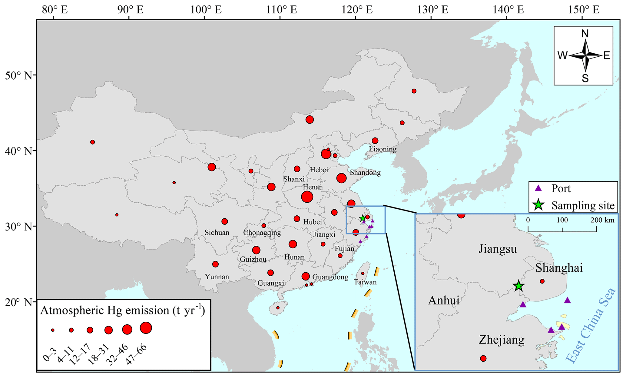
Figure 1 The location of the Dianshan Lake (DSL) site in Shanghai, China. The red dots in the map represent the anthropogenic atmospheric Hg emissions by each province in 2014 (Wu et al., 2016).

2.2 Measurements of atmospheric mercury

GEM, GOM, and PBM were measured from June 2015 to May 2016 using the Tekran 2537B/1130/1135 system (Tekran Inc., Canada), an instrument that has been widely used worldwide (Landis and Keeler, 2002). In general, GEM, GOM, and PBM in the atmosphere were collected by dual gold cartridges, a KCl-coated annular denuder, and a regenerable quartz fiber filter, respectively. In this study, GEM was collected at an interval of 5 min with a flow rate of 1 L min⁻¹, while GOM and PBM were collected at an interval of 2 h with a flow rate of 10 L min⁻¹. After the collection, all mercury species were thermally decomposed to Hg⁰ immediately and measured by cold vapor atomic fluorescence spectroscopy (CVAFS). GEM concentrations were expressed in nanograms per cubic meter, while GOM and PBM were in picograms per cubic meter at a standard temperature of 273.14 K and pressure of 1013 hPa.

Quality control procedures are strictly followed. The KCl-coated denuder, Teflon-coated glass inlet, and impactor plate were replaced weekly and quartz filters were replaced monthly. Before sampling, denuders and quartz filters were prepared and cleaned according to the methods in Tekran technical notes. The Tekran 2537B analyzer was routinely calibrated using its internal permeation source every 47 h, and was also cross-calibrated every 3 months against an external temperature-controlled Hg vapor standard. Two-point calibrations (including zero calibration and span calibration) were performed separately for each pure gold cartridge. Manual injections were performed to evaluate these automated calibrations using the standard saturated mercury vapor. Extremely high concentrations (especially for GOM and PBM) were occasionally observed. If the values were several times higher than the previous hour, those data were regarded as outliers and were excluded in the data analysis.

2.3 Measurements of other air pollutants and meteorological parameters

Water-soluble inorganic anions (${\mathrm{SO}}_{\mathrm{4}}^{\mathrm{2}-}$, ${\mathrm{NO}}_{\mathrm{3}}^{-}$, Cl⁻) and cations (K⁺, Mg²⁺, Ca²⁺, ${\mathrm{NH}}_{\mathrm{4}}^{+}$) in PM_2.5 were simultaneously monitored by the Monitor for Aerosols and Gases in ambient Air (MARGA) at the resolution of 1 h. Ambient air was drawn into a sampling box at a flow rate of 16.7 L min⁻¹. After removing the water-soluble gases by an absorbing liquid, a supersaturation of water vapor induced the particles in the airflow to grow into droplets, and then the droplets were collected and transported into the analytical box, which contains two ion chromatograph systems for the determination of the water-soluble ions in PM_2.5.

Heavy metals (Pb, Fe, K, Ba, Cr, Se, Cd, Ag, Ca, Mn, Cu, As, Hg, Ni, Zn, V) in PM_2.5 were measured hourly using the Xact 625 ambient metals monitor (Cooper Environmental, Beaverton, OR, USA), which is a sampling and analyzing X-ray fluorescence spectrometer designed for online measurements of particulate elements. In this study, ambient air was sampled at a flow rate of 16.7 L min⁻¹ and the particles were collected onto a Teflon filter tape. Then the filter tape was moved into the spectrometer, where it was illuminated with an X-ray tube under three excitation conditions and the excited X-ray fluorescence was measured by a silicon drift detector. Daily advanced quality assurance checks were performed for 30 min after midnight to monitor shifts in the calibration.

The hourly meteorological data including air temperature, relative humidity (RH), wind speed, and wind direction were simultaneously monitored at the observation site by the automatic weather station (AWS). The data of planetary boundary layer (PBL) height were retrieved from the US National Oceanic and Atmospheric Administration (https://ready.arl.noaa.gov/READYamet.php, last access: 1 May 2019). Atmospheric ozone (O₃) concentration was continuously measured using a Thermo Fisher 49i, which operates on the principle that ozone molecules absorb UV light at a wavelength of 254 nm. The ambient carbon monoxide (CO) and PM_2.5 concentrations were measured by a Thermo Fisher 48i-TLE and Thermo Fisher 1405-F, respectively. All the data were averaged into hour values.

2.4 Potential source contribution function (PSCF)

PSCF is a useful tool to diagnose the possible source areas with regard to the levels of air pollutants when setting a contamination concentration threshold at the receptor site. Back trajectory models are used to simulate the airflows. The principle of PSCF is to calculate the ratio of the total number of back trajectory segment endpoints in a grid cell (i, j) exceeding the threshold concentration (m_ij) to the total number of back trajectory segment endpoints in this grid cell (i, j) during the whole sampling period (n_ij) (Eq. 1) (Schroeder and Munthe, 1998; Cheng et al., 2015):

$$\begin{array}{}\text{(1)}& {\displaystyle }{\displaystyle }{\mathrm{PSCF}}_{ij}={\displaystyle \frac{m_{ij}}{n_{ij}}}.\end{array}$$

When a particular cell is associated with a small number of endpoints, a weighting function (w_ij) is applied to reduce this uncertainty and the value of w_ij is shown in Eq. (2) (Fu et al., 2011), in which N_avg is the mean n_ij of all grid cells with n_ij greater than zero. PSCF_ij is multiplied by w_ij to derive the weighted PSCF values.

$$\begin{array}{}\text{(2)}& {\displaystyle }{\displaystyle }{w}_{ij}=\left\{\begin{array}{cl}\mathrm{1.0},& N_{ij}>\mathrm{3}{N}_{\mathrm{ave}}\\ \mathrm{0.7},& \mathrm{3}{N}_{\mathrm{ave}}>N_{ij}>\mathrm{1.5}{N}_{\mathrm{ave}}\\ \mathrm{0.4},& \mathrm{1.5}{N}_{\mathrm{ave}}>N_{ij}>N_{\mathrm{ave}}\\ \mathrm{0.2},& N_{\mathrm{ave}}>N_{ij}\end{array}\right.\end{array}$$

In this study, we set the threshold concentration as the mean value of the whole sampling period. The mean GEM, PBM, and GOM concentrations were 2.77 ng m⁻³, 60.8 pg m⁻³, and 82.1 pg m⁻³, respectively. The HYSPLIT (HYbrid Single-Particle Lagrangian Integrated Trajectory) model is applied for calculating air mass backward trajectories (Stein et al., 2015). The model was run online at the NOAA ARL READY website using the meteorological data archives of the Air Resource Laboratory (ARL). The meteorological input data used in the model were obtained from the NCEP (National Centers for Environmental Prediction) Global Data Assimilation System (GDAS) with a horizontal resolution of 0.5^∘ × 0.5^∘. In this study, 72 h back trajectories were calculated at 500 m a.g.l. (above ground level) and the cell size was set as 0.5^∘ × 0.5^∘.

2.5 Positive matrix factorization (PMF)

The PMF model is widely used to quantitatively determine the source contributions of specific air pollutants (Gibson et al., 2015). The essential principle of PMF is that the concentration of each sample is determined by source profiles and different contributions. The equation of the PMF model is shown as Eq. (3):

$$\begin{array}{}\text{(3)}& {\displaystyle }{\displaystyle }{X}_{ij}=\sum _{k=\mathrm{1}}^P{g}_{ik}{f}_{kj}+e_{ij},\end{array}$$

where X_ij is the concentration of the jth contamination at the receptor site in the ith sample. g_ik represent the contribution of the kth factor on the ith sample, f_kj is used to express the mass fraction of the jth contamination in the kth factor, P is the number of factors, which represent pollution sources, and e_ij is the residual for each measurement or model error.

Before the model determines the optimal non-negative factor contributions and factor profiles, an objective function, which is the sum of the square difference between the measured and modeled concentrations weighted by the concentration uncertainties, has to be minimized (Cheng et al., 2015). The equation that determines the objective function is given by Eq. (4):

$$\begin{array}{}\text{(4)}& {\displaystyle }{\displaystyle }Q=\sum _{i=\mathrm{1}}^n\sum _{j=\mathrm{1}}^m{\left({\displaystyle \frac{X_{ij}-\sum _{k=\mathrm{1}}^p{A}_{ik}{F}_{kj}}{S_{ij}}}\right)}^{\mathrm{2}},\end{array}$$

where X_ij is the ambient concentration of the jth pollutant in the ith sample (m and n represent the total number pollutants and samples, respectively). A_ik is the contribution of the kth factor on the ith sample and F_kj is the mass fraction of the jth pollutant in the kth factor. S_ij is the uncertainty of the jth pollutant on the ith measurement, and P is the number of factors, which imply the pollutant sources. In this study, the number of factors from three to eight was examined with the optimal solutions determined by the slope of the Q value versus the number of factors. For each run, the stability and reliability of the outputs were assessed by referring to the Q value, residual analysis, and correlation coefficients between observed and predicted concentrations. Finally, a six-factor solution, which showed the most stable results and gave the most reasonable interpretation, was chosen. Before running the model, a dataset including unique uncertainty values of each data point was created and digested into the model. The error fraction was assumed to be 15 % of concentrations for GEM and 10 % of concentrations for the other compounds (Xu et al., 2017); the missing data were excluded and the total number of samples was 3526.

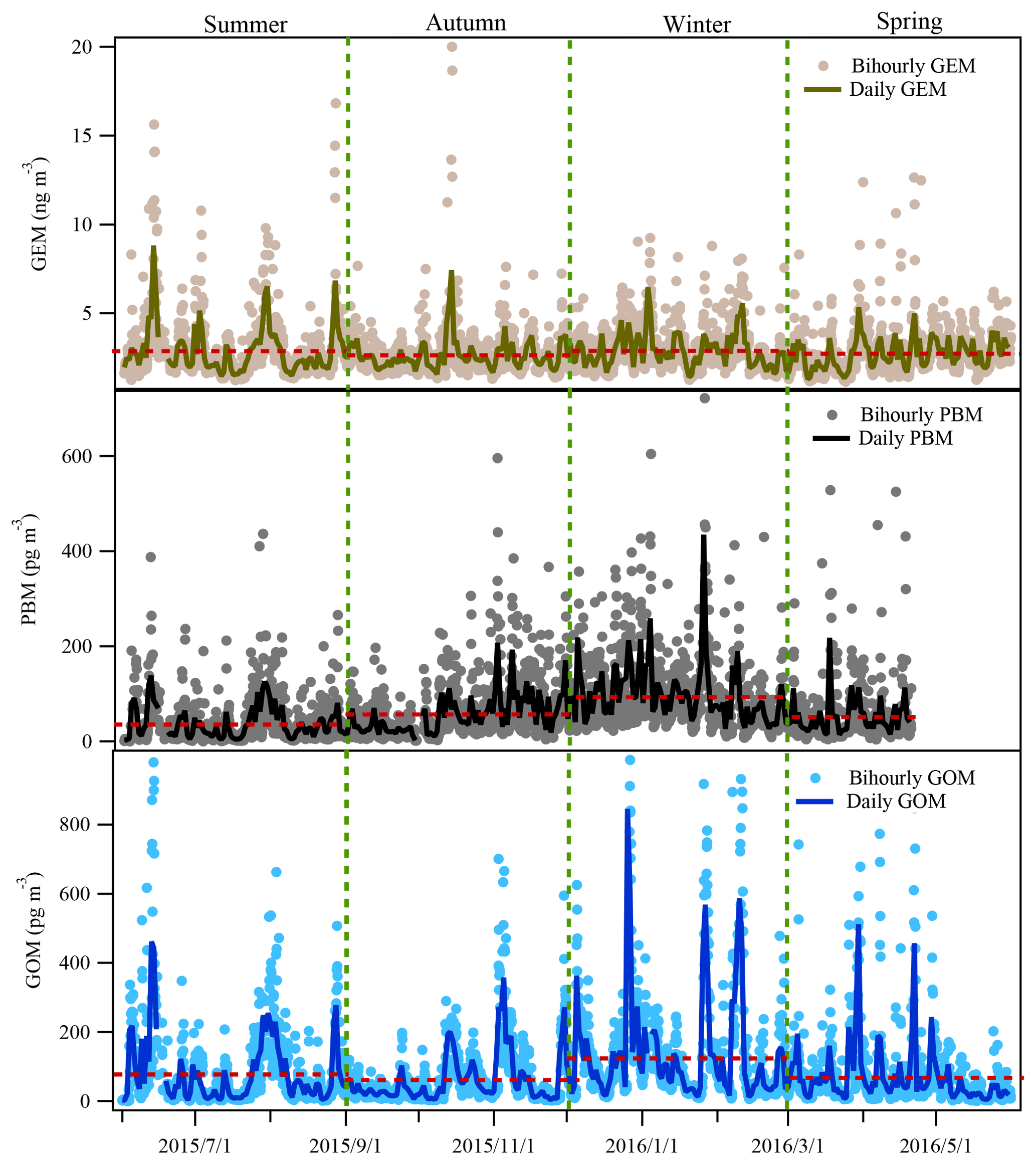
Figure 2 Time series of atmospheric Hg (GEM, PBM, and GOM) concentrations during the whole study period at DSL. The red dashed lines represent the mean concentrations of Hg species in each season.

3 Results and discussion

3.1 Characteristics of atmospheric mercury species

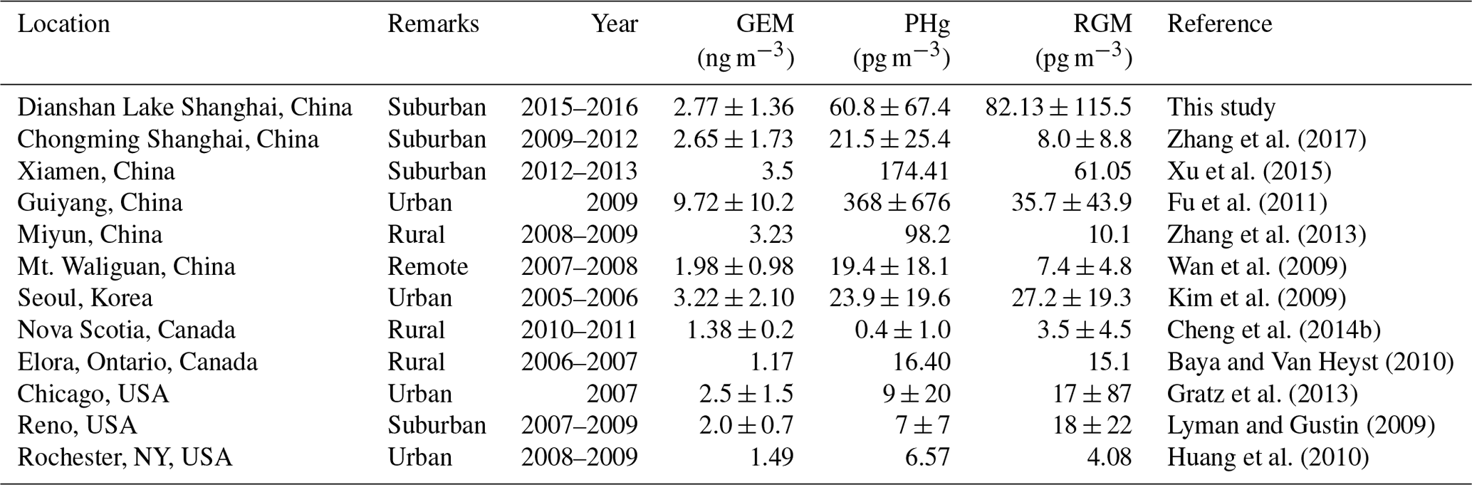
Figure 2 displays the time series of atmospheric GEM, PBM, and GOM concentrations from 1 June 2015 to 31 May 2016 at DSL. The annual average concentrations of GEM, PBM, and GOM at DSL were 2.77±1.36 ng m⁻³, 60.8±67.4 pg m⁻³, and 82.1±115.4 pg m⁻³, respectively. As shown in Table 1, the levels of GEM and PBM in this study were lower than at some sites in China by a factor of 2–7, such as rural Miyun, suburban Xiamen, and urban Guiyang (Xu et al., 2015; Fu et al., 2011). However, compared to the studies conducted in urban and rural areas abroad such as New York (Wang et al., 2009), Chicago (Gratz et al., 2013), and Nova Scotia (Cheng et al., 2014b), the concentrations of GEM and PBM in the suburbs of Shanghai were much higher by a factor of 1–3 and 3–8, respectively. Different from GEM and PBM, the GOM concentrations at DSL were higher than at all the other Chinese sites and sites around the world listed in Table 1. The mean GOM concentration in this study (82.1 pg m⁻³) was even higher than that in Guiyang (35.7 pg m⁻³), where the emissions of GEM and GOM were quite intense due to the massive primary emission sources such as coal-fired power plants and cement plants (Fu et al., 2011). The abnormally high GOM concentrations observed in this study were likely dominated by strong primary emissions.

Table 1 The concentrations of speciated atmospheric mercury in this study and at other sites around the world.

The monthly patterns of GEM, PBM, and GOM during the whole sampling period are shown in Fig. 3. The seasonal mean GEM concentrations were slightly higher in winter (2.88 ng m⁻³) and summer (2.87 ng m⁻³) than in spring (2.73 ng m⁻³) and autumn (2.63 ng m⁻³), with the highest monthly mean value of 3.19 ng m⁻³ in June and the lowest of 2.39 ng m⁻³ in March. Statistical tests showed that no significant differences of the seasonal variations in GEM concentrations among spring, summer, and winter were observed (Table S2). This was different from many urban and remote sites in China, such as Guiyang, Xiamen, and Mt. Changbai, where GEM showed significantly higher concentrations in cold than warm seasons (Wang et al., 2016; Xu et al., 2015; Fu et al., 2012). The relatively high GEM concentrations during the cold season in China should be attributed to the increases in energy consumption (Fu et al., 2015). In this study, GEM concentration in summer was comparable to that in winter, which was likely attributed to the strong natural mercury emissions (e.g., soils, vegetation, and water) due to the elevated temperature in summer (Liu et al., 2016). The seasonal mean PBM concentrations were the highest in winter (93.5 pg m⁻³), the lowest in summer (35.7 pg m⁻³), and moderate in autumn (56.8 pg m⁻³) and spring (51.6 pg m⁻³), with the highest monthly mean value of 109.4 pg m⁻³ in January and the lowest of 28.9 pg m⁻³ in September. This seasonal pattern was consistent with those at the other sites in China such as Beijing and Nanjing (Kim et al., 2009; Lynam and Keeler, 2005). PBM concentrations at low-altitude sites in the Northern Hemisphere were commonly enhanced in winter, which was ascribed to intense emissions from residential heating, the reduction of wet scavenging processes, enhanced gas–particle partitioning of atmospheric mercury under low temperature, etc. (Rutter and Schauer, 2007). As for GOM, its seasonal mean concentrations were the highest in winter (124.0 pg m⁻³), followed by summer (77.3 pg m⁻³), spring (68.1 pg m⁻³), and autumn (61.0 pg m⁻³). GOM concentrations in summer were much lower than those in winter, but were higher than in spring and autumn. Secondary transformation from GEM in warm/hot seasons and slow dispersion in winter can explain such season variations, as further discussed below.

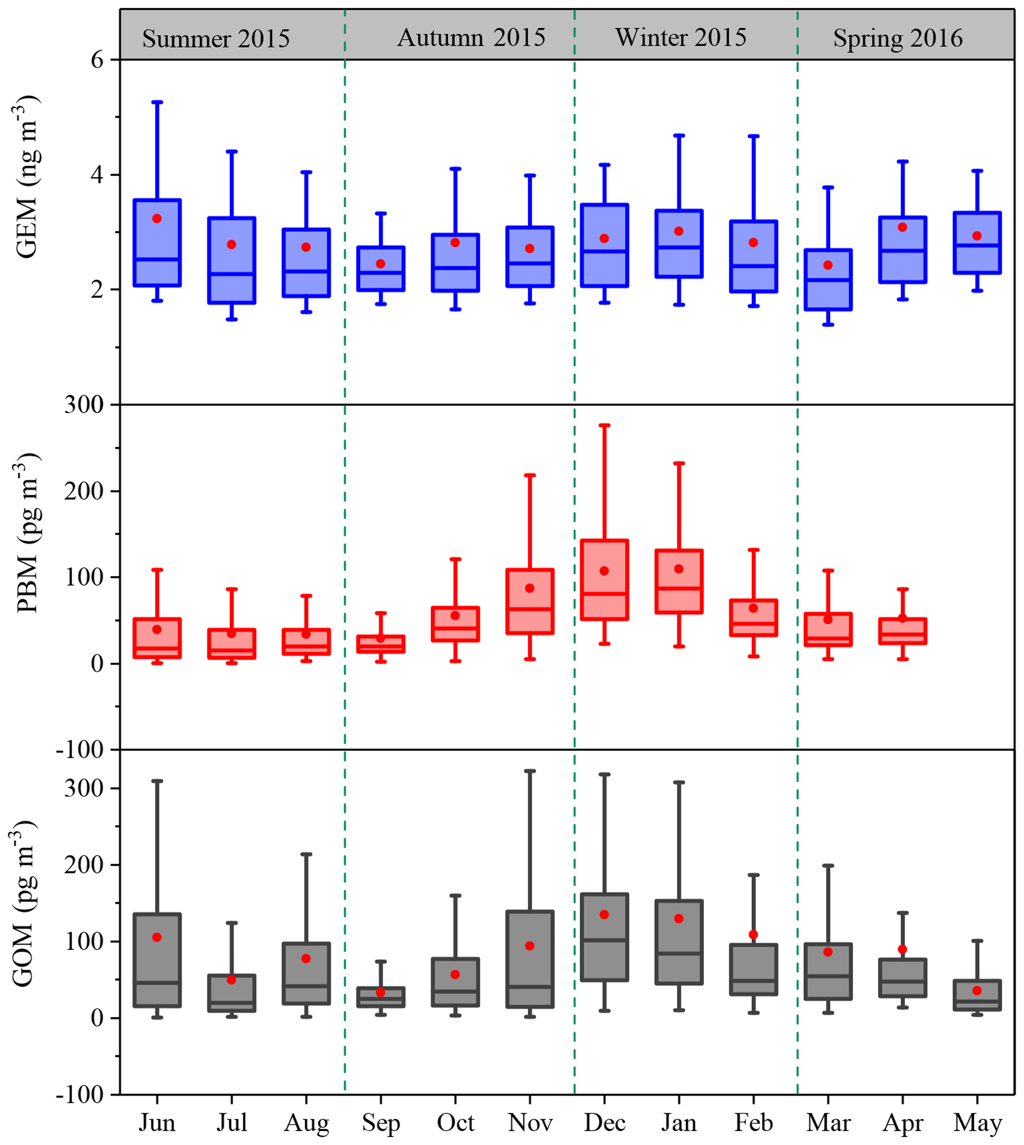
Figure 3 Monthly variation in GEM, PBM, and GOM concentrations. The 10th, 25th, median, 75th, and 90th percentile values are indicated in the box plots. The red dots represent the mean values.

Figure 4 shows the diurnal variations in GEM, PBM, and GOM during the whole sampling period. To ensure the time resolutions were consistent among all the three mercury species, the temporal resolution of measured GEM was converted from 5 min to the 2 h average. As shown in Fig. 4, GEM concentrations were higher during daytime with the maximum in the morning at around 10:00 LT and minimum at midnight around 02:00 LT. The diurnal trends of GOM were similar to those of GEM, except that the minimum GOM occurred at around 20:00 LT in the evening. The diurnal trends of PBM were different from those of GEM and GOM, exhibiting relatively higher concentrations during nighttime. The PBM maximum occurred in the early morning at around 06:00 LT and the minimum in the afternoon at 18:00 LT. The diurnal trends of GEM, PBM, and GOM were similar to those observed in Nanjing (Zhu et al., 2012), but different from those in Guiyang, Xiamen, and Guangzhou (Wang et al., 2016; Chen et al., 2013). Since DSL and Nanjing both belong to the Yangtze River Delta region, the similar meteorology and emission characteristics within the Yangtze River Delta region may explain the similar diurnal patterns of Hg species between these two sites. The elevated GEM concentrations at DSL during daytime were likely related to the stronger emissions from both human activities and natural releases. GOM and GEM showed similar diurnal variations and both peaked at 10:00 LT, probably suggesting that GOM and GEM were affected by common sources (e.g., coal-fired power plants and industrial boilers). The high PBM concentrations at night were likely derived from the adsorption of Hg species onto the preexisting particles and the subsequent accumulation in the shallow nocturnal boundary layer. Wind speed was relatively low while relative humidity was high at night, which were conducive to the adsorption of GOM onto the particles (Fig. 4).

Figure 4 Annual mean diurnal variation in GEM, PBM, and GOM concentrations.

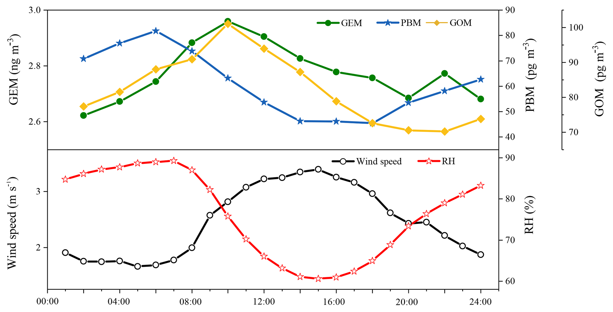
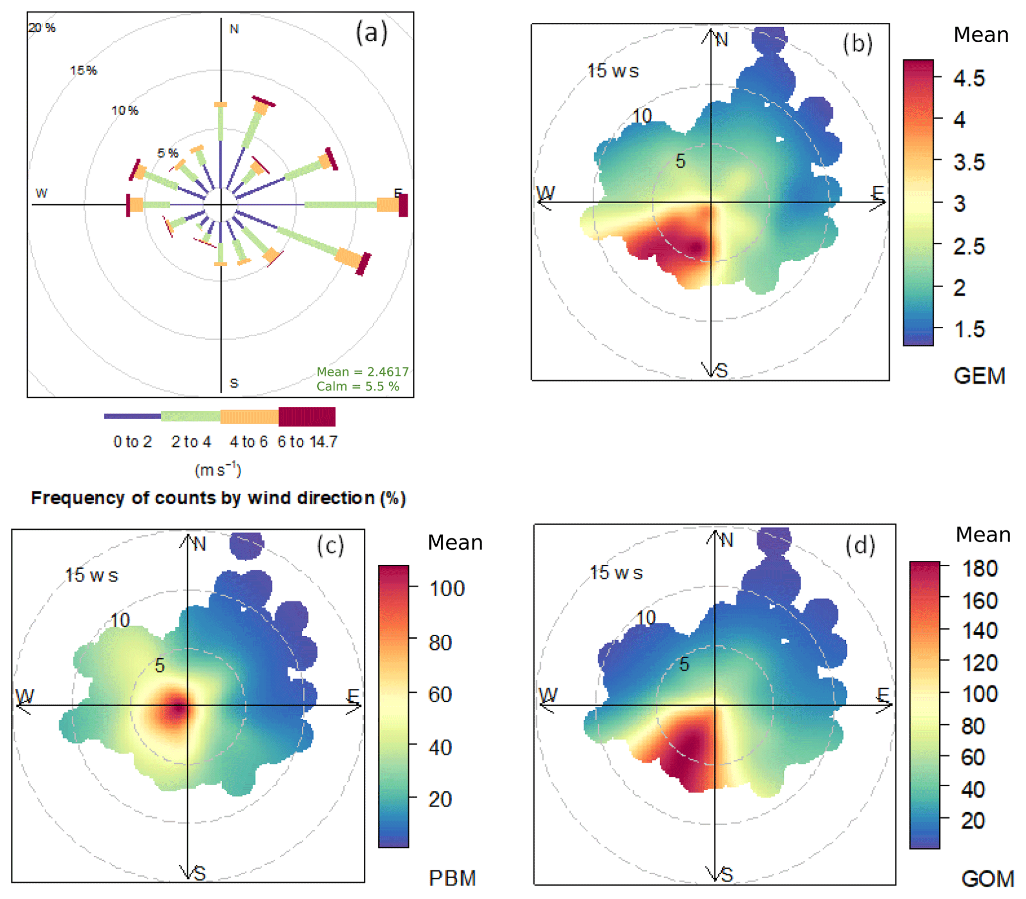
Figure 5 (a) Wind rose plot during the study period. Mean concentrations of (b) GEM, (c) PBM, and (d) GOM as a function of wind speed and wind directions. The radii of the circle in (a) represent the frequency of wind directions and the radii of the circle in (b–d) represent the value of wind speed.

3.2 Relationship between Hg species and meteorological factors

Figure 5 shows the relationship between wind direction–speed and atmospheric mercury species. One-third of the prevailing winds came from the east and 16 % from the north at DSL during the study period (Fig. 5a). Wind speed from all directions during the study period was mainly in the range of 0–6 m s⁻¹, of which wind speed higher than 4 m s⁻¹ mainly derived from the east. The highest GEM concentrations, averaged at 3.92 ng m⁻³, were linked to the winds from the south and southwest, in comparison to the average concentration of 2.71 ng m⁻³ from the other wind sectors (Fig. 5b). A similar wind–concentration pattern was also seen for GOM, but not for PBM for which high concentrations were from the north-northwest and south-southwest (Fig. 5c and d). Anthropogenic emissions were generally higher in northern than southern China (Fig. 1), which largely explained the observed high concentrations from the north wind sector. However, even higher atmospheric Hg concentrations were observed from the south and southeast wind sector, implying other factors dominated the Hg concentrations in these wind sectors. Wang et al. (2016) reported that Hg concentrations in the surface soils were generally higher in southern than northern China. A modeling study estimated that the mean annual Hg air–soil flux in the southwest region of our sampling site (e.g., Zhejiang Province) ranged from 8.75 to 15 ng m⁻² h⁻¹, while that in the north-northwest region (e.g., Jiangsu Province) ranged from 2.5 to 8.75 ng m⁻² h⁻¹ (Wang et al., 2016). Hence, emissions from natural sources, such as soils, vegetation, and water, should play important roles in the observed high atmospheric Hg concentrations from the south to southeast wind sectors.

In order to confirm this hypothesis, the relationship between temperature and Hg concentrations at DSL was investigated. Seasonal temperature in ascending order was divided into different groups and the corresponding mean Hg concentrations are plotted in Fig. 6. In spring, GEM concentration increased with increasing temperature. In the other seasons, similar trends were observed when temperature increased to a certain value. Such a phenomenon was likely caused by temperature-dependent surface emissions, noting that the increasing PBL height with increasing temperature should have offset some of the increased mercury concentration. GOM concentration showed a clearly positive correlation with temperature in summer, largely due to the in situ oxidation of GEM under high-temperature heavy ozone pollution (Qin et al., 2018). Such a good correlation did not exist in the other seasons. As for PBM, it appeared to have weakly negative correlation with PBL height, suggesting the atmospheric diffusion conditions were influential on the concentrations of PBM.

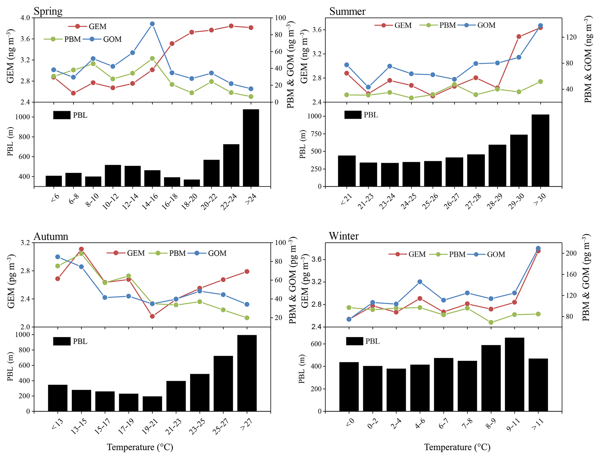
Figure 6 The variation in atmospheric Hg (GEM, PBM, and GOM) and PBL as a function of temperature in all four seasons.

3.3 Source apportionment analyses

3.3.1 Potential source regions for mercury

PSCF analysis results suggested that the potential sources for GEM were mainly located in Anhui, Jiangxi, and Zhejiang provinces, and also possibly in Shandong Province (Fig. 7a). Seasonal dominant sources affecting GEM at the DSL site were those in Jiangsu and Zhejiang provinces in spring, in Anhui and Jiangxi provinces in summer, in Jiangsu Province in autumn, and in Anhui and Zhejiang provinces in winter (Fig. S1 in the Supplement). In addition, sources in Henan and Shandong provinces seemed to also play a role in GEM in winter, suggesting the importance of long-range transport in this season. There were substantial high PSCF signals in the southern areas, stronger than those in the northern areas, despite lower anthropogenic emissions in the south. For example, southern provinces such as Zhejiang and Jiangxi were estimated to release 25 t yr⁻¹ of atmospheric Hg from anthropogenic activities (Fig. 1), far less than those from the northern provinces such as Jiangsu and Shandong (77 t yr⁻¹) (Wu et al., 2016). Based on the mean annual Hg air–soil flux of 8.75 to 15 ng m⁻² h⁻¹ in the southwest region of our sampling site (Wang et al., 2016), it was estimated that the total Hg emissions from soils were in the range of 6.9–13.9 t yr⁻¹ from Zhejiang Province, which was comparable to the anthropogenic Hg emissions of approximately 15 t yr⁻¹ in 2014 in this province (Wu et al., 2016). Thus, the soil emissions of GEM from natural surfaces was an importance source in southern areas, corroborating the discussion in Sect. 3.2. In addition, the East China Sea (including the offshore areas and open ocean) showed sporadic high PSCF signals of GEM in all the four seasons (Fig. S1), indicating possible influences from shipping activities (more discussion below).

Figure 7 Potential source regions of atmospheric Hg (GEM, PBM, and GOM) at the observational site according to PSCF analysis.

The PSCF pattern of PBM was quite different from that of GEM (Fig. 7b). The annual potential source regions for PBM were mainly from the northern areas of Jiangsu and Anhui provinces and from northeastern China including Shandong and Hebei provinces. These provinces were regarded as the main Hg sources areas in China and accounted for approximately 25.2 % of the Chinese anthropogenic atmospheric Hg emissions (Wu et al., 2016). Seasonal sources for PBM were similar in spring, autumn, and winter, but not in summer, for which high PSCF values were mainly located in the southern areas of Shanghai, likely due to the prevailing winds in summer from the south, southeast, and southwest where Zhejiang and Jiangxi provinces were important mercury source regions.

The annual potential sources for GOM were mainly located in Anhui and Zhejiang provinces and the coastal areas along Jiangsu Province (Fig. 7c). The PSCF pattern of GOM was similar to that of GEM but not PBM. The potential source regions of GOM were more from southern than northern China, likely due to the higher atmospheric oxidant levels in the southern regions. Seasonal PSCF patterns for GOM showed dominant sources in Zhejiang and Jiangxi provinces in summer, major sources in inland areas and moderate sources over the East China Sea and Yellow Sea in spring, major sources in Zhejiang Province and moderate sources over the Yellow Sea in autumn, and major sources from the coastal areas of Jiangsu to the vast Yellow Sea in winter. One previous study suggested that the marine boundary layer could provide considerable amounts of oxidants such as chlorine and bromine, which were beneficial for the production of GOM by oxidizing GEM (van Donkelaar et al., 2010) and this mechanism may explain the substantial PSCF signals over the ocean.

The PSCF analysis results discussed above demonstrated the relative contributions from the short-range transport from the adjacent areas of Shanghai and regional and long-range transport from northern and southern China as well as from the ocean on contributing to speciated atmospheric mercury at DSL (more discussion below).

3.3.2 Quasi-local sources versus regional/long-range transport on atmospheric mercury

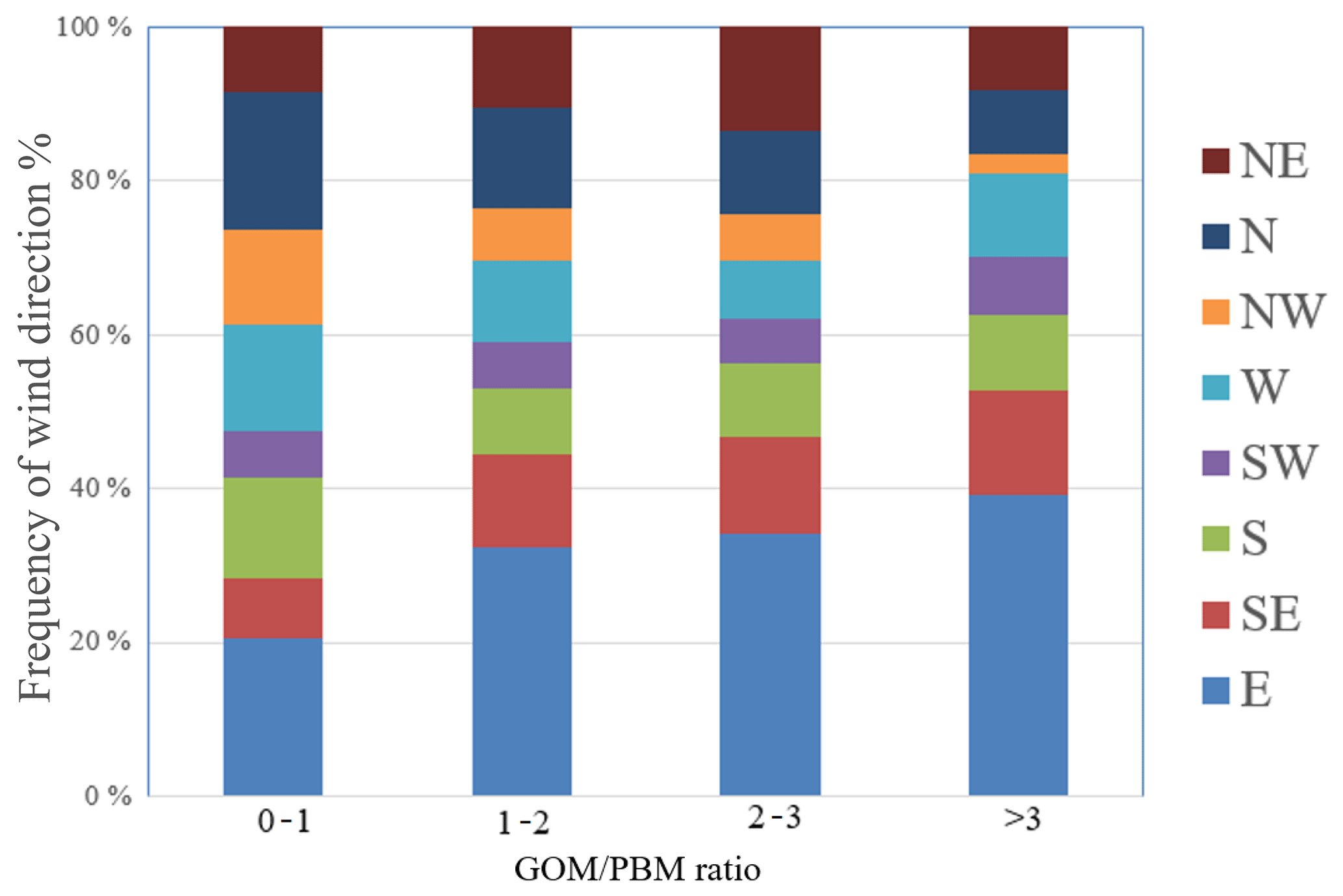
According to the relationships between wind direction and Hg concentration as well as the PSCF analysis results discussed above, the elevated GEM, GOM, and PBM concentrations at DSL were generally associated with the wind sectors from the southwest and north directions. To reveal the relative importance of local sources and regional transport, the ratio of GOM ∕ PBM was applied as an indicator based on the fact that the residence time of GOM is generally considered to be shorter than that of PBM (Lee et al., 2016). Lower ratios of GOM ∕ PBM indicate the dominance of regional/long-range transport over local sources, and vice versa. In the following discussion, the ratios of GOM ∕ PBM during the whole study period were grouped into four categories, i.e., 0–1, 1–2, 2–3, and higher than 3, with their corresponding wind sector distribution shown in Fig. 8. Higher GOM ∕ PBM ratios were mostly associated with winds from the east and southeast, e.g., with the frequency of these two wind sectors increasing from 27 % for the GOM ∕ PBM ratios of less than 1 to 52 % for the ratios higher than 3. Winds from these wind sectors were typically characterized by relatively clean air masses, suggesting the dominance of local sources over the regional transport at the observational site. In contrast, lower GOM ∕ PBM ratios were mostly associated with winds clockwise from the west to the north, with the frequency of these wind sectors decreasing significantly from 44 % for the GOM ∕ PBM ratios less than 1 to 21 % for the ratios higher than 3, indicating the importance of the long-range/regional transport from northern China associated with the relatively low GOM ∕ PBM ratios. According to the PSCF results above, the potential source areas of Hg species (GEM, GOM, and PBM) derived mostly from the south and southwest of the sampling site. As shown in Fig. 8, the frequency of south, southwest, west, and northeast winds showed no clear trend as the GOM ∕ PBM ratios increased, suggesting complicated interactions that cannot be explained solely by the local sources or regional transport. In general, the GOM ∕ PBM ratio can be used as a qualitative tracer for identifying the relative importance of long-range transport vs. local sources if one factor dominates over the other.

Figure 8 Frequency of wind directions under different ranges of GOM ∕ PBM ratios.

The relationships among GEM, CO, secondary inorganic aerosols (SNAs), and GOM ∕ PBM ratio were further investigated. Figure 9 displays the concentrations of GEM as a function of GOM ∕ PBM ratio colored by CO. The size of the circles represents the corresponding concentration of SNA in PM_2.5. CO has been commonly used as a tracer of fuel combustion, and SNAs were derived from secondary particle formation via the gas-to-particle conversion. CO and SNA were collectively used as proxies of the extent of regional/long-range transport of anthropogenic air pollutants. As shown in Fig. 9, GEM generally increased with increasing GOM ∕ PBM ratio. In addition, lower GOM ∕ PBM ratios were associated with higher CO and SNA concentrations and vice versa. This corroborated the discussion above that the GOM ∕ PBM ratio was a reliable tracer for assessing the relative importance of regional/long-range transport vs. local atmospheric processing.

GEM concentration fluctuated with a mean value of less than 2.6 ng m⁻³ when the GOM ∕ PBM ratio was less than 2.5, increased from 2.61 ng m⁻³ in the GOM ∕ PBM ratio bin of 2.5–3.0 to 2.8 ng m⁻³ in the bin of 3.0–3.5, and then remained relatively stable when the GOM ∕ PBM ratio was higher than 3.0. Generally, GEM showed an increasing trend as the GOM ∕ PBM ratio increased while both SNA and CO decreased. The elevated GEM concentrations tended to be associated with quasi-local sources. In contrast, under the high-SNA and high-CO conditions and when GOM ∕ PBM ratios were lower, GEM showed relatively low concentrations, suggesting that regional/long-range transport did not favor the elevation of GEM concentration. It has been recognized that the common regional/long-range transport pathways contributing to the particulate pollution events in Shanghai were from the north and northwest, which originated mostly from the North China Plain. The relatively lower GEM concentrations under the regional/long-range transport conditions corroborated the PSCF analysis that only moderate probabilities of GEM source regions were from northern China (Fig. 7a).

Figure 9 The GEM concentrations as a function of the GOM ∕ PBM ratios in each bin of 0.5. The dots are colored by the concentrations of CO, and the sizes of the dots represent the concentrations of SNA in PM_2.5. The bars represent 1 standard error of GEM concentration in each bin.

3.3.3 Source apportionment by the combined PMF and PCA

PMF modeling has been widely used to apportion the sources of atmospheric pollutants. In this study, GEM together with heavy metals and soluble ions, measured online synchronously, were introduced into the EPA PMF5.0 model to apportion the major anthropogenic sources of GEM. A six-factor solution was selected based on the results of multiple model runs, which can explain the measured concentrations of the introduced species well. The profiles of the six identified PMF factors and contributions of major anthropogenic sources to GEM are shown in Fig. 10. It has to be noted that since no tracers for the natural emissions (e.g., soil, vegetation, and ocean) were available in this study, the identification of natural mercury sources was not possible based on the PMF modeling.

Figure 10 A six-factor source apportionment for anthropogenic GEM based on PMF analysis.

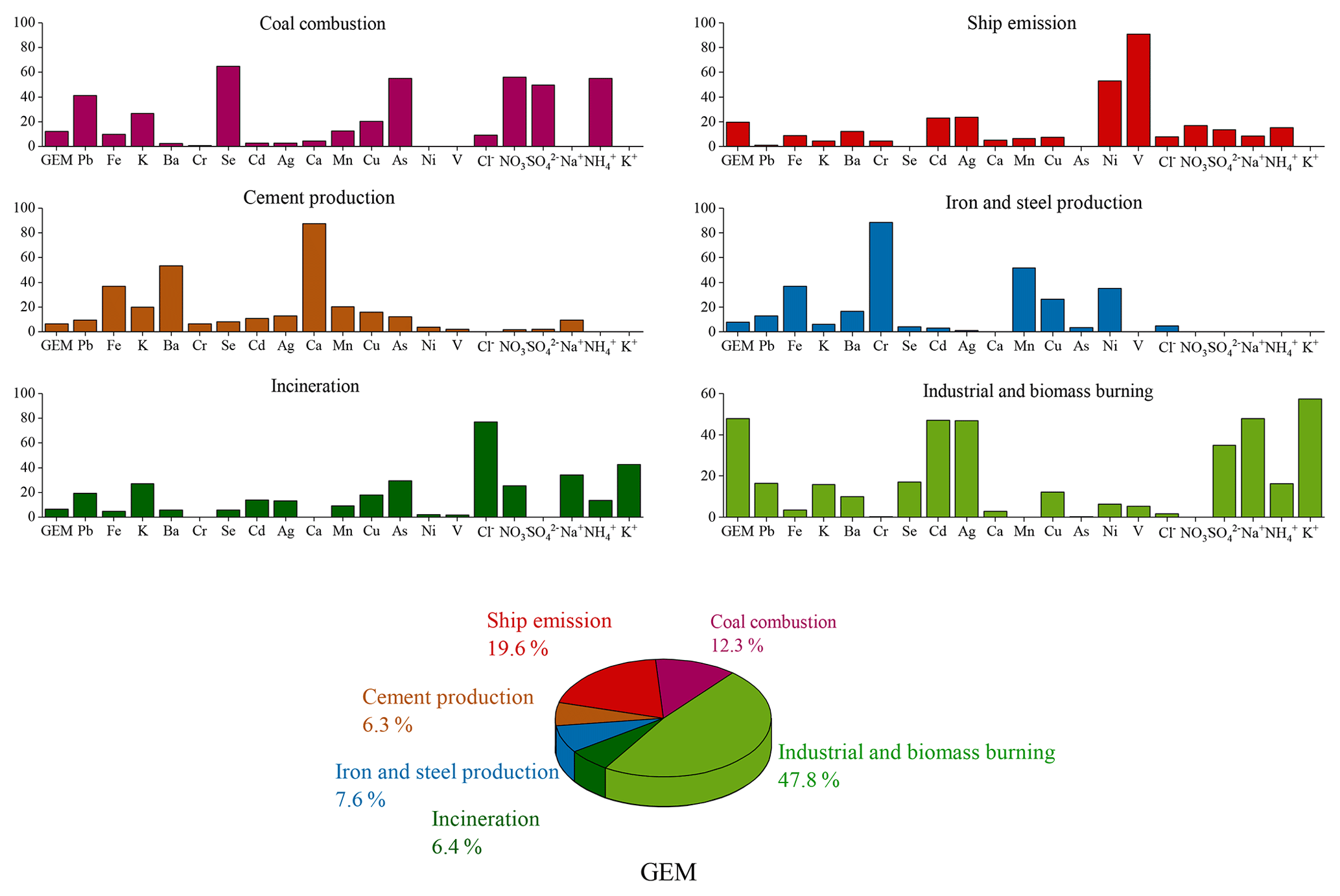
Factor 1 had high loadings of Se, As, Pb, ${\mathrm{NO}}_{\mathrm{3}}^{-}$, ${\mathrm{SO}}_{\mathrm{4}}^{\mathrm{2}-}$, and ${\mathrm{NH}}_{\mathrm{4}}^{+}$. Se, As, and Pb were typical tracers of coal combustion. ${\mathrm{SO}}_{\mathrm{4}}^{\mathrm{2}-}$ and ${\mathrm{NO}}_{\mathrm{3}}^{-}$ were also formed from the gaseous pollutants emitted from coal burning. Hence, this factor was defined as coal combustion sources and accounted for 12.3 % of the anthropogenic GEM. Figure S4 plotted wind roses of specific aerosol species. ${\mathrm{SO}}_{\mathrm{4}}^{\mathrm{2}-}$ and As shared similar patterns with high concentrations mainly from the southwest. Since combustion was an important source of GEM, this confirmed that the major sources of GEM were located in the southwest region.

Factor 2 displayed particularly high loadings of Ni and V. The major sources of Ni in the atmosphere can be derived from coal and oil combustions (Tian et al., 2012), and oil combustion accounted for 85 % of anthropogenic V emissions in the atmosphere (Duan and Tan, 2013). In general, Ni and V have been considered good tracers of heavy oil combustion, which has been commonly used in marine vessels (Viana et al., 2009). Thus, this factor was identified as shipping emissions. The sampling site is adjacent to the East China Sea and is located in Shanghai, which has the largest port in the world. Figure S4 showed similar patterns of Ni and V with high concentrations mainly from the northeast, east, and southeast. To further validate this factor, the time series of GEM concentrations from the shipping factor based on the PMF modeling were extracted and digested into the PSCF modeling (Fig. S5), which showed that the potential source regions were mainly located over the East China Sea and coastal regions. This indicated a factor of 2 from PMF should be representative of the shipping sector as well as oil combustion in motor vehicles and inland shipping activities. Overall, this factor accounted for 19.6 % of anthropogenic GEM and ranked as the second largest emission sector, highlighting the urgent need of controlling the marine vessel emissions.

Factor 3 showed high loadings of Ca and moderate loadings of Ba and Fe. Ca and Fe are rich in the crust and can be used for cement production. As mercury could be released during industrial processes of cement production, Factor 3 was assigned as cement production and accounted for a minor fraction of 6.3 % of the anthropogenic GEM.

Factor 4 was characterized by high loadings of Cr and moderate loadings of Mn, Fe, Ni, and Cu. These species together served as markers of metal smelting. Metal smelting is known to emit large sources of Hg to the atmosphere (Pirrone et al., 2010), especially in the YRD, one of the most developed and industrialized areas in China. This factor accounted for 7.6 % of the anthropogenic GEM.

Factor 5 had high loadings of Cl⁻. Waste incineration is an important source of enriched chloride over land. Factor 5 was identified to be waste incineration, which contributed 6.4 % of the anthropogenic GEM.

Factor 6 was characterized by high loadings of Cd, Ag, K⁺, and Na⁺. The major sources of Cd in China were the iron and steel smelting industries (Duan and Tan, 2013). Ag was mainly used in industrial applications, including electronic appliances and photographic materials. K⁺ was a typical tracer of biomass burning, which often stemmed from agriculture waste burning over the Yangtze River Delta and the North China Plain. Factor 6 was considered a combined source of the industrial and biomass burning emission sectors. It was estimated to contribute 47.8 % of the anthropogenic GEM.

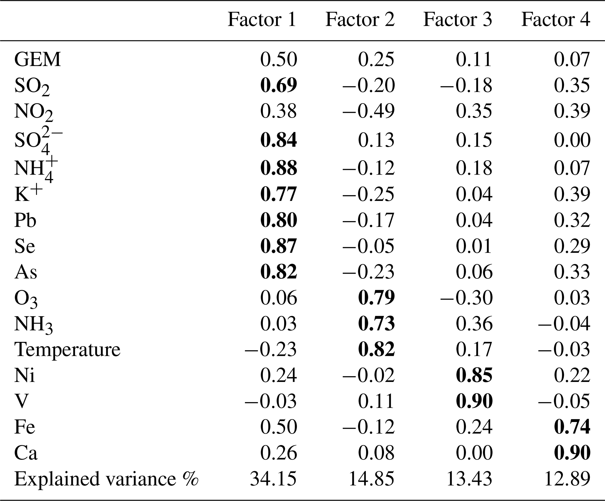
As discussed above, surface emissions were likely to be important sources of the observed atmospheric mercury. As PMF modeling did not resolve the natural sources of mercury, PCA (principal component analysis) was applied for further source apportionment by introducing the temperature parameter. Four factors are resolved, which totally explained 75.32 % of the variance as shown in Table 2. Factor 1 accounted for 34.15 % of the total variance with high loadings for SO₂, ${\mathrm{SO}}_{\mathrm{4}}^{\mathrm{2}-}$, ${\mathrm{NH}}_{\mathrm{4}}^{+}$, K⁺, Pb, Se, and As, which was explained as coal combustion mixed with biomass burning. Factor 2 accounted for 14.85 % of the total variance with high loadings for temperature, O₃, and NH₃, which was explained as surface emissions. Factor 3 accounted for 13.43% of the total variance and showed high loadings for Ni and V, which indicated the contribution of ship emissions. Factor 4 accounted for 12.89 % of the total variance and showed high loadings for Fe and Ca, indicating the contribution of cement production.

Table 2 PCA (principal component analysis) for GEM at DSL. Note that bold values represent high loading (factor loading > 0.50).

3.4 Factors affecting the formation and transformation of mercury species

3.4.1 Factors affecting the formation of GOM

A typical case from 24 to 27 July 2015 was chosen to investigate the possible formation process of GOM. As shown in Fig. 11, the shaded episodes represented nighttime from 18:00 to 06:00 LT the next day. Both GEM and GOM exhibited rising trends during nighttime (Fig. 11a), which was ascribed to the nighttime accumulation effect due to the very shallow boundary layer (Fig. 11c). Starting from 06:00 LT in the morning, GEM concentration began to gradually decline as the boundary layer developed. In contrast, the concentration of GOM continued to rise from 06:00 LT until it reached the peak value at around 10:00 LT. During this period, ozone and temperature also kept rising until they surpassed 200 µg m⁻³ and 34 ^∘C, respectively. Accordingly, as an anthropogenic emitting tracer, the concentration of carbon monoxide was basically stable and even showed a downward trend, which suggested that some other factors caused the increase in GOM in addition to the anthropogenic emissions. This phenomenon clearly revealed the acceleration of the conversion process of GEM to GOM under favorable atmospheric conditions of higher O₃ concentration and ambient temperature. In the case of atmosphere dilution by the rise of PBL, the fact that GOM was not falling but rising suggested the great influence of this process on ambient GOM concentration. Similar observation has been found at the high-altitude Pic du Midi observatory in southern France (Fu et al., 2016), which was almost impervious to anthropogenic emission sources. The important role of GEM oxidation at our sampling site, which is located in one of the most developed industrial areas in China, was most likely due to the presence of sufficient oxidants in this area. Severe ozone pollution frequently occurred in the YRD due to strong anthropogenic emission intensities (Duan et al., 2017). Previous studies suggested that the primary oxidants in the terrestrial environment were O₃ and OH radicals (Zhang et al., 2015), while Br was an important oxidant in the subtropical marine boundary layer (Obrist et al., 2011). It was possible that, in addition to O₃ and OH radicals, Br might also be an important species to oxidize GEM as the DSL site is adjacent to the East China Sea.

Figure 11 A case study of GEM oxidation from 24 to 27 July 2015. The time series of GEM, GOM, O₃, CO, temperature, and PBL are plotted. The shaded parts represent nighttime.

Statistical relationships among GOM, O₃, and temperature are shown in Fig. 12. Temperature was plotted against a range of GOM ∕ PBM bins colored by O₃ and the size of the circles represents the concentration of GOM. In general, as temperature and O₃ increased, the concentration of GOM was subject to substantial enhancement. For instance, when temperature (O₃) was below 12 ^∘C (65.7 µg m⁻³), GOM was averaged at 37.8 pg m⁻³. While temperature (O₃) increased to above 20 ^∘C (91.5 µg m⁻³), GOM rose to 168.8 pg m⁻³, yielding a factor of 1–5 increases. This further confirmed the hypothesis from the case study above that the levels of oxidants under favorable environmental conditions were crucial for the formation of GOM. It can also be seen from Fig. 12 that the lower ratios of GOM ∕ PBM were associated with lower temperatures and O₃ concentrations, indicating relatively weak photochemistry during the cold seasons. On the contrary, the higher ratios of GOM ∕ PBM were associated with higher temperature and O₃ concentrations, indicating relatively strong photochemistry during the warm seasons. Thus, the formation of GOM was more favored by local atmospheric processing rather than the transport. This study demonstrated the abnormally high GOM concentrations observed at DSL were largely ascribed to local oxidation reactions. However, the explicit formation mechanism of GOM needs to be investigated by measuring more detailed components of GOM and atmospheric oxidants.

Figure 12 Temperature variations in each bin of the GOM ∕ PBM ratios. The dots are colored by the concentrations of O₃ and the sizes of the dots represent the concentrations of GOM. The bars represent 1 standard error of temperature in each bin.

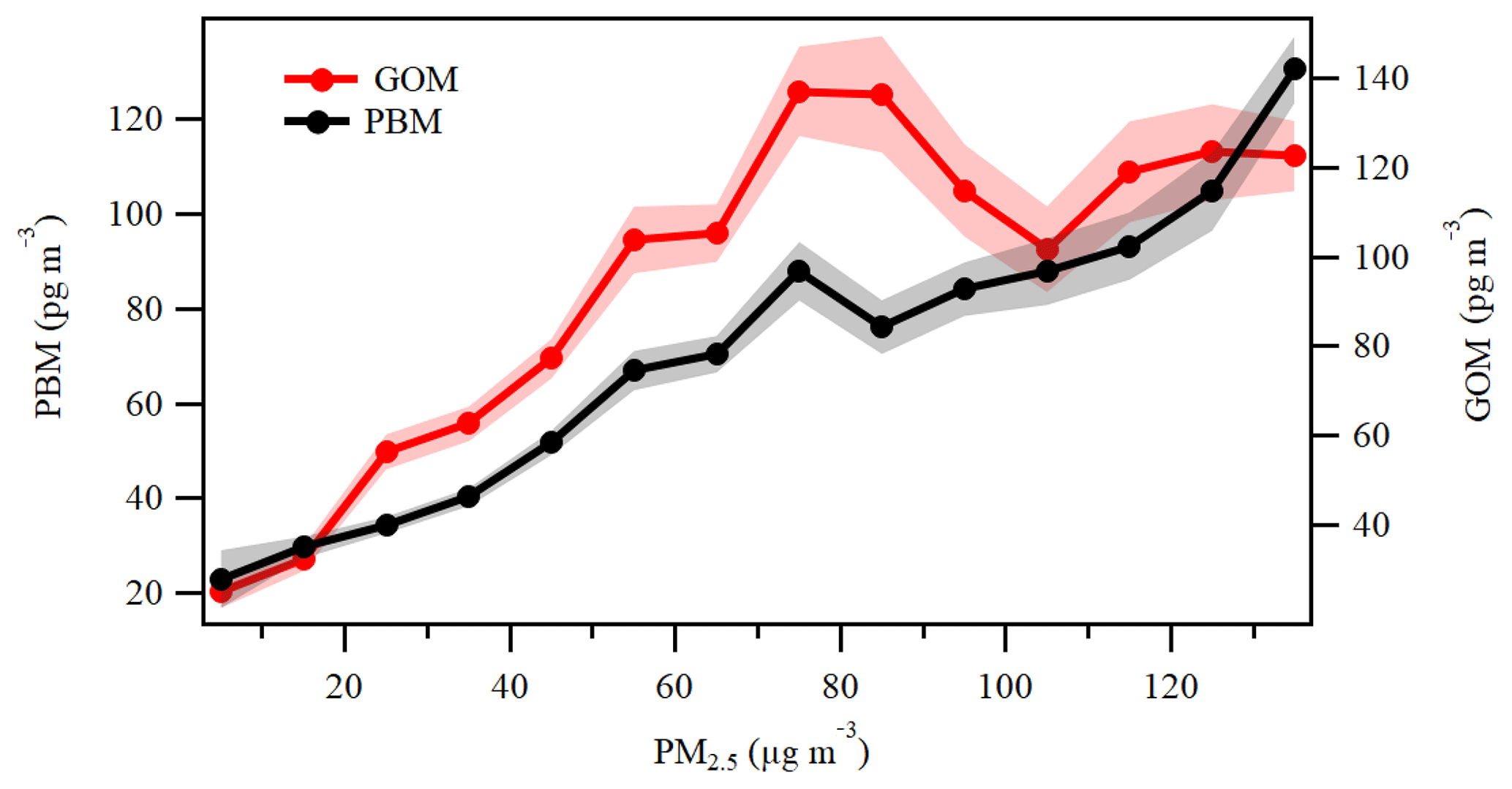
Figure 13 The variations in PBM and GOM as a function of PM_2.5 in each bin of 10 µg m⁻³. The shaded areas represent 1 standard error of GOM and PBM concentrations.

Figure 14 A case study of gas–particle portioning between GOM and PBM from 30 December 2015 to 1 January 2016, which was divided into different stages. The time series of PBM, GOM, PM_2.5, CO, temperature, and RH are plotted.

3.4.2 Factors affecting the transformation of PBM

Previous studies have shown that PBM can be emitted directly from various anthropogenic sources such as coal-fired power plants and industries (Cheng et al., 2014a; Wu et al., 2016). In addition, gas–particle partitioning was considered to be an important pathway for the formation of PBM (Zhang et al., 2015; Amos et al., 2012). Since most of the areas in the YRD belong to non-attainment areas in regard to particulate pollution and the concentrations of GOM were particularly high at DSL as discussed above, the role of gas–particle partitioning in the formation of PBM should be investigated. Previous studies reported that the concentrations of PM_2.5 in eastern and northern China are the highest in the world (van Donkelaar et al., 2010), for which the elevated atmospheric particulate matter probably facilitates the formation of PBM (Fu et al., 2015). Figure 13 shows the statistical pattern of the variation in PBM and GOM in the ascending bins of PM_2.5. The concentration of PBM increased with increasing PM_2.5, likely due to the gas–particle portioning of oxidized Hg (Amos et al., 2012; Cheng et al., 2014a). The trend of GOM was somehow different from that of PBM. When PM_2.5 concentrations were at relatively low levels under 75 µg m⁻³, GOM concentrations increased with PM_2.5. However, when PM_2.5 concentrations increased to 75–105 µg m⁻³, GOM exhibited a clear decreasing trend as PM_2.5 increased. This suggests that low levels of PM_2.5 may not have an apparent effect on GOM, but higher levels of PM_2.5 may directly affect GOM through adsorption of GOM onto the particles. When PM_2.5 concentrations exceeded 105 µg m⁻³, GOM exhibited a slightly increasing trend as PM_2.5 increased. High PM_2.5 concentrations in China always related to severe anthropogenic emissions (van Donkelaar et al., 2010), so the moderate increasing trend of GOM in these bins should be attributed to the impact of strong primary emissions.

A short episode from 30 December 2015 to 1 January 2016 was chosen to further investigate this phenomenon. As shown in Fig. 14, in Stage 1, the concentrations of PM_2.5 were below 100 µg m⁻³, and PBM and GOM share similar temporal variation to PM_2.5. In Stage 2, as PM_2.5 kept climbing, GOM began to show somewhat negative correlation with PM_2.5, but not significant. The reason might be that the relatively high temperature and low humidity during this period were not conducive to the transfer of GOM to particle matters. In Stage 3, GOM decreased as PM_2.5 continued to increase, showing a clear anticorrelation. During this period, PBM showed a consistent trend with PM_2.5 and CO. Temperature was relatively low but with relatively high humidity. This phenomenon clearly demonstrated the process of gas–particle partitioning of PBM formation. In Stage 4, GOM and PBM showed a similar decreasing trend as PM_2.5 and CO. The low GOM concentrations, low humidity, and high temperature resulted in no significant signs of GOM adsorption to PM_2.5 in this stage. In general, under high PM_2.5, GOM concentration and humidity, and low-temperature conditions at DSL, clear processes of gas–particle partitioning were observed.

4 Conclusions

In this study, a year-long observation of speciated atmospheric Hg concentrations was conducted at the Dianshan Lake (DSL) Observatory, located on the typical transport routes from mainland China to the East China Sea. Different from many sites in China, GEM at DSL exhibited high concentrations in winter, summer, and spring, which was due to the strong re-emission fluxes from natural surfaces in summer and enhanced coal combustion for residential heating over northern China in winter. The relatively high GOM concentrations in summer indicated that the formation of GOM from GEM oxidation was likely crucial. PBM exhibited high concentrations in winter, indicating the impact of long-range transport. The diurnal patterns of GEM and GOM were similar with relatively high levels during daytime. For GEM, this was likely attributed to both human activities and re-emission from natural surfaces during daytime. For GOM, in addition to direct emissions, high concentrations during daytime were partially ascribed to photochemical oxidation of GEM. The PBM concentrations were higher during nighttime, which was ascribed to the accumulation effect within the shallow nocturnal boundary layer.

The relationship between meteorological factors and atmospheric Hg species showed that the high Hg concentrations were generally related to the winds from the south, southwest, and north and positively correlated with temperature. Both anthropogenic sources and natural sources contributed to the atmospheric mercury pollution at DSL. Higher GOM ∕ PBM ratios corresponded to lower CO and SNA concentrations and vice versa. The ratio of GOM ∕ PBM can be used as a tracer for distinguishing local sources and regional/long-range transport based on the fact that the residence time of GOM was shorter than that of PBM. GEM as a function of the GOM ∕ PBM ratio indicated that when the quasi-local sources dominated, GEM concentrations were relatively higher than those events under the regional/long-range transport conditions. According to the PMF source apportionment results, six sources of anthropogenic GEM and their contributions were identified, i.e., industrial and biomass burning (47.8 %), shipping emissions (19.6 %), coal combustion (12.3 %), iron and steel production (7.6 %), incineration (6.4 %), and cement production (6.3 %). The significant contribution of shipping emissions suggested that in coastal areas mercury emitted from marine vessels can be significant. In addition, a considerable natural source of GEM was identified by including temperature into the principle component analysis.

The formation processes of GOM and PBM based on episodic studies were also investigated. The high GOM concentrations were partially attributed to strong local photochemical reactions under the conditions of high O₃ and temperature. Under high PM_2.5 concentration and humidity and low-temperature conditions, the gas–particle partitioning processes were observed.