the Creative Commons Attribution 4.0 License.
the Creative Commons Attribution 4.0 License.
 | 30 Apr 2019
Heuristic estimation of low-level cloud fraction over the globe based on a decoupling parameterization
Jihoon Shin
Based on the decoupling parameterization of the cloud-topped planetary boundary layer, a simple equation is derived to compute the inversion height. In combination with the lifting condensation level and the amount of water vapor in near-surface air, we propose a low-level cloud suppression parameter (LCS) and estimated low-level cloud fraction (ELF), as new proxies for the analysis of the spatiotemporal variation of the global low-level cloud amount (LCA). Individual surface and upper-air observations are used to compute LCS and ELF as well as lower-tropospheric stability (LTS), estimated inversion strength (EIS), and estimated cloud-top entrainment index (ECTEI), three proxies for LCA that have been widely used in previous studies. The spatiotemporal correlations between these proxies and surface-observed LCA were analyzed.
Over the subtropical marine stratocumulus deck, both LTS and EIS diagnose seasonal–interannual variations of LCA well. However, their use as a global proxy for LCA is limited due to their weaker and inconsistent relationship with LCA over land. EIS is anti-correlated with the decoupling strength more strongly than it is correlated with the inversion strength. Compared with LTS and EIS, ELF and LCS better diagnose temporal variations of LCA, not only over the marine stratocumulus deck but also in other regions. However, all proxies have a weakness in diagnosing interannual variations of LCA in several subtropical stratocumulus decks. In the analysis using all data, ELF achieves the best performance in diagnosing spatiotemporal variation of LCA, explaining about 60 % of the spatial–seasonal–interannual variance of the seasonal LCA over the globe, which is a much larger percentage than those explained by LTS (2 %) and EIS (4 %).
Our study implies that accurate prediction of inversion base height and lifting condensation level is a key factor necessary for successful simulation of global low-level clouds in general circulation models (GCMs). Strong spatiotemporal correlation between ELF (or LCS) and LCA identified in our study can be used to evaluate the performance of GCMs, identify the source of inaccurate simulation of LCA, and better understand climate sensitivity.
- Article
(11614 KB) - Full-text XML
-
Supplement
(1516 KB) - BibTeX
- EndNote


Clouds belong to the most important but uncertain components of the climate system. Due to their strong shortwave radiative cooling effect on the Earth, low-level clouds have been the focus of various studies in the past few decades, both in the observation and modeling communities. Slingo (1990) estimated that a 4 % increase in the low-level cloud amount (LCA) has the potential to offset global warming associated with a doubled CO2 concentration. Most low-level clouds exist over the ocean, mainly due to abundant moisture sources near the surface (Hahn and Warren, 1999). Among various types of low-level clouds, marine stratocumulus clouds (MSCs) have received special attention due to their large spatial coverage and the complexity of physics and dynamic processes controlling their formation and dissipation (Wood, 2012). Several planetary boundary layer (PBL) schemes used in general circulation models (GCMs) have the capability to simulate MSCs and associated feedback processes in a realistic way (e.g., Lock et al., 2000; Bretherton and Park, 2009; Park and Bretherton, 2009). However, MSCs simulated by these parameterization schemes or more complex numerical models are the results of complex interactions among various physics processes. Therefore, it has not been easy for the climate researchers to understand the feedback processes of MSCs from the climate perspective. If a simple proxy could diagnose spatial and temporal variations of MSCs, it would be much easier for the climate researcher to understand the role of MSCs in future climate, both qualitatively and quantitatively.
Klein and Hartmann (1993) (KH93 hereafter) showed that a lower-tropospheric stability (LTS) where θ700 and θ1000 are the potential temperatures at 700 and 1000 hPa levels, respectively, correlates well with seasonal variations of LCA over the subtropical marine stratocumulus deck. LTS has been widely used as a proxy to understand the characteristics of MSCs and their impact on future climate. The success of LTS stems in part from the fact that LTS is correlated with other factors controlling the formation of MSCs in the subtropical marine stratocumulus deck such as the sea surface temperature (SST), cold air advection, free-tropospheric moisture, and subsidence in association with a subtropical high-pressure system. Using a heuristic Lagrangian MSC model, Park et al. (2004) (PLR04 hereafter) explored the sensitivity of MSCs to various environmental conditions in the cold advection regime of the northeastern subtropical Pacific and to both warm and cold advection regimes of the eastern equatorial Pacific Ocean. Consistent with Klein (1997), PLR04 found a positive correlation between the simulated MSC fraction and strong upstream subsidence, although Myers and Norris (2013) reported the opposite correlation. PLR04 simulated less MSCs with a drier free atmosphere. However, enhanced longwave radiative cooling at the top of MSCs capped by a drier free atmosphere (this process was not included in the PLR04's model) may increase MSCs by enhancing turbulent vertical moisture transport from the sea surface to overlying MSCs.
Based on the decoupling hypothesis suggested by PLR04 and other proceeding works (e.g., Augstein et al., 1974; Albrecht et al., 1979; Betts and Ridgway, 1988; Bretherton, 1992), Wood and Bretherton (2006) (WB06 hereafter) extended KH93's LTS and suggested an estimated inversion strength (EIS) as a better proxy for LCA in which temperature profiles in the decoupled layer below the inversion and the free troposphere above the inversion are assumed to be close to a moist adiabat that is strongly temperature-dependent. WB06 showed that, compared with LTS, EIS correlates better with LCA over a wide range of stratocumulus regimes, because it captures the lapse rate and boundary layer structure more completely than LTS. Similar to LTS, EIS has been widely used as a good proxy for LCA.
In their derivation of EIS, WB06 assumed that the factor , where zinv is the inversion height and and are the moist adiabatic lapse rates at 700 hPa and lifting condensation level (LCL) of near-surface air (zLCL), respectively, contributes less to the correlation relationship between the inversion strength and LTS than the other terms, so that it was simply set to zero. Although a scaling argument was provided to justify this simplification, a more fundamental reason for neglecting this term was associated with the practical difficulty in estimating and parameterizing zinv. PLR04 suggested a heuristic parameterization for PBL decoupling to simulate stratocumulus cloudiness in the inversion-capped marine boundary layer. In their study, PBL decoupling is parameterized as an increasing function of the height difference between zinv and zLCL. PLR04's conceptual idea of PBL decoupling was used in WB06's derivation of EIS and other studies to understand the variation of cloudiness associated with PBL decoupling (Stevens, 2006; Xiao et al., 2011; Van der Dussen et al., 2014, 2015, 2016; Park, 2014a, b; Dal Gesso et al., 2015a, b; Neggers et al., 2017). In our study, we suggest a simple heuristic method to estimate zinv by combining PLR04's decoupling parameterization with EIS. By using zinv, zLCL, and water vapor specific humidity in the surface-based mixed layer (qv,ML), we propose two low-level cloud suppression parameters (LCS), and with Δzs=2750 m, and an estimated low-level cloud fraction, with , as new proxy for the characterization of the spatiotemporal variation of LCA over the globe. Individual surface and upper-air observations are used to compute LTS, EIS, LCS, and ELF, and the correlations between these proxies and the surface-observed seasonal LCA are examined. We also analyzed the recently proposed estimated cloud-top entrainment index (ECTEI, Kawai et al., 2017), which is a modified EIS that takes into account cloud-top entrainment criteria. It will be shown that, compared with LTS, EIS, and ECTEI, which are mainly designed as proxies for marine LCA, ELF and LCS are better proxies for the global LCA, applicable over both the ocean and land.
The structure of this paper is as follows. Section 2.1 provides a detailed explanation on the conceptual framework used to compute zinv, LCS, ELF, and other related proxies for LCA. Section 2.2 describes the data and analysis method. The correlations between various proxies and LCA in spatial and temporal domains over the globe are presented in Sect. 3. A summary and conclusion are provided in Sect. 4.
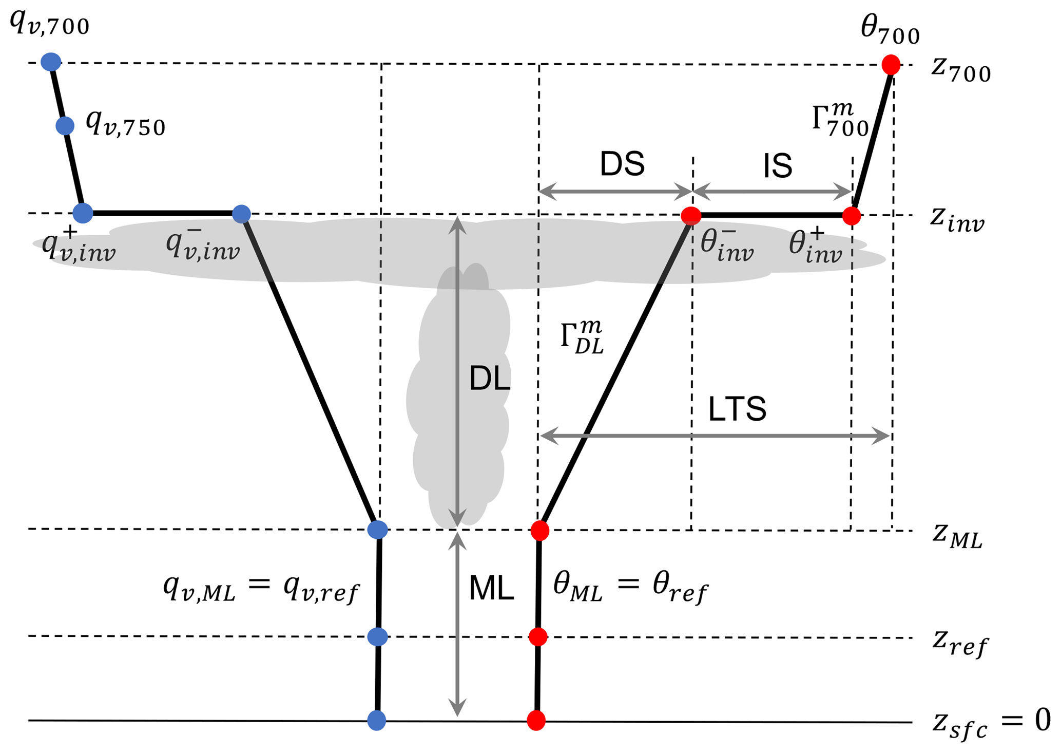
Figure 1Schematic diagram illustrating an idealized structure of the decoupled planetary boundary layer (PBL), which consists of a surface-based mixed layer (ML) topped by zML with the potential temperature, θML=θref, and water vapor specific humidity, , given at the reference height, zref; a decoupled layer (DL) in which the vertical temperature gradient is assumed to follow a saturated moist adiabat at the ML top (); an inversion at zinv across which θ increases and qv decreases in a discontinuous way; and the free atmosphere between zinv and z700 in which the vertical temperature gradient is assumed to follow a saturated moist adiabat at the 700 hPa level (). Also shown are the inversion strength, IS ; decoupling strength, DS ; and lower-tropospheric stability (LTS) . The lapse rate of qv in the free atmosphere is given by the linear slope between qv,700 and qv,750. For simplicity, it is assumed that θ and qv share a common decoupling parameter, . Over the ocean, stratocumulus generally exists below the inversion base and shallow cumulus grows into the overlying stratocumulus in the decoupled layer. See the text for more details.
2.1 Conceptual framework
Following PLR04 and WB06, we assume that the lower troposphere below 700 hPa consists of four regimes (see Fig. 1): a surface-based mixed layer (ML) topped at zML with the potential temperature, θML, and water vapor specific humidity, qv,ML, specified at the reference height, zref or pref (i.e., θML=θref, ); a decoupled cloud layer (DL) with a vertical gradient of θ approximated by the moist θ adiabat at zML (); an inversion at the DL top (zinv); and the free atmosphere with a vertical gradient of θ approximated by the moist θ adiabat at p=700 hPa (). The moist adiabatic lapse rate of θ used in our study ( and in unit of K m−1) is a function of T and p; it increases as p increases or T increases. The inversion strength at zinv, IS , becomes
where is the potential temperature just above the inversion, is the potential temperature just below the inversion, and LTS is the lower-tropospheric stability. By assuming that the contribution of to variability in the relationship between IS and LTS is negligibly small due to the opposite variations of zinv and with LTS, WB06 derived the so-called estimated inversion strength, EIS:
which was shown to be a better proxy for LCA than LTS. Because it does not contain zinv, which is hard to estimate, EIS has been used as a convenient proxy for LCA.
If zinv can be reasonably estimated instead of being neglected, it may be possible to construct a better proxy than EIS for LCA. In this study, we suggest an approach to estimate zinv and other related proxies in a heuristic way based on the decoupling hypothesis suggested by PLR04. From the analysis of sounding data, PLR04 showed that the decoupling parameter α can be parameterized as an increasing function of the decoupled layer thickness, ,
where the scale height, Δzs≈2750 m, is obtained from the analysis of a set of sounding data over the ocean (see PLR04). Originally, PLR04 defined α for the condensate potential temperature with γ≈1.1–1.3, where ql and qi are the cloud liquid and ice contents, respectively, and θc is a conserved scalar with respect to the phase change. In our study, however, α is defined for θ and, accordingly, γ is slightly reduced to 1 to account for in the cloud-topped decoupled layer. The choice of γ=1 allows us to obtain analytical expressions for various proxies as will be shown below. The small (large) α indicates that the environmental air at the inversion base, , is well connected to (decoupled from) the surface air property with abundant moisture, providing more (less) favorable conditions for the formation of LCA at . It should be noted that α only measures the degree of vertical decoupling of thermodynamic properties between zML and . That is, α does not provide information regarding the amount of surface moisture.
By combining Eq. (3) with and , we can derive the following expressions for the inversion height,
which can be also written as from Eq. (3). Then, the inversion strength, IS, becomes
and decoupling strength, DS , becomes
and , as shown in Fig. 1. Once θML=θref, , and zML are obtained, we can consecutively compute and zinv using the first expression of Eq. (4), α from Eq. (3), IS from Eq. (5), and DS from Eq. (6). Note that IS is identical to the sum of EIS and , the neglected term in the original formulation of WB06.
Following previous studies (e.g., PLR04 and WB06), we will assume that zML≈zLCL over the ocean. However, due to insufficient moisture at the surface, it is likely that zML<zLCL over most land areas unless strong buoyancy or shear production near the surface sufficiently deepens the surface-based mixed layer. It may be possible to parameterize zML as a function of turbulent kinetic energy within the PBL; however, for simplicity, we assume that zML≈zLCL over the entire globe.
As mentioned above, α only measures the degree of vertical decoupling of thermodynamic properties between the inversion base and surface air, not the surface moisture itself. Conceptually, however, the formation of LCA at the inversion base is likely to be influenced by both surface moisture and α. As a simple but practical proxy representing surface moisture, we select zLCL. From the simple conceptual argument that small (large) zLCL and α are likely to be associated with large (small) LCA at the inversion base, we define the first low-level cloud suppression parameter (LCS), β1, as
where the second equality is obtained by assuming zML≈zLCL and μ=2. In principle, μ can be estimated in an empirical way using multiple linear regression analysis of LCA fitted to zinv and zLCL such that β1 explains the maximum fraction of the variance of LCA. We performed a multiple linear regression analysis of LCA on zinv and zLCL using individual seasonal data in each 2.5∘ latitude × 5∘ longitude grid box over the globe. Except over some portions, the values of μ were mostly between 0 and 4 with an approximate average value, μ=2 (not shown). The resulting β1 is a non-dimensional sum of zinv and zLCL. By simply extending β1, we also define the second LCS, β2, as a non-dimensional product of zinv and zLCL,
which, similar to β1, increases as the surface air becomes drier and the PBL deepens. In the case of zML≈zLCL, it becomes and , where the first factor in both formulae represents the degree of subsaturation of near-surface air, and the second factor represents the decoupling strength. Note that zLCL oppositely controls the surface moisture parameter and decoupling strength: small zLCL decreases the first factor but increases the second factor and vice versa. Large (small) values of β1 and β2 likely favor the dissipation (formation) of LCA at the inversion base.
Finally, we define the estimated low-level cloud fraction (ELF) as
where f is the freeze-dry factor (Vavrus and Waliser, 2008),
designed to reduce the parameterized cloud fraction in the extremely cold and dry atmospheric conditions typical of polar and high-latitude winter. Cloud fraction parameterization based on the grid-mean relative humidity (RH) assumes that there is a certain amount of subgrid variability of thermodynamic scalars (e.g., Park et al., 2014), which allows the formation of cloud fraction even when the grid-mean RH is smaller than 1. In the very stable Arctic and high-latitude atmosphere during winter, however, there is little subgrid variability (Jones et al., 2004). Thus, any grid-mean RH-based cloud fraction parameterization (e.g., our LCS based on zLCL) is likely to predict too much LCA there. Vavrus and Waliser (2008) showed that the implementation of the freeze-dry factor into GCMs substantially reduced the simulated LCA in the Arctic and high-latitude regions during winter and improved the simulation. Compared to β2, ELF diagnoses smaller LCA in the high-latitude region during winter where the amount of water vapor within the ML is often smaller than 3 g kg−1 (see Fig. 2e, f). If zML≈zLCL, it becomes , where f denotes the amount of water vapor in the surface-based ML air, zLCL represents the degree of subsaturation of near-surface air, and quantifies the degree of thermodynamic decoupling of the inversion base air from the surface-based ML air. Our ELF predicts that LCA increases as the near-surface air becomes more saturated with enough water vapor and as the PBL becomes more vertically coupled. When the inversion base air is fully coupled with saturated near-surface air containing enough water vapor, ELF approaches its upper bound of 1. Considering that low-level clouds usually form at zinv, the conceptual cloud formation processes embedded in ELF are consistent with what is expected to happen in nature. We defined ELF using β2 instead of β1, because β2 has a better global performance than β1 (see Tables 1, 3, 4, 6). Note that our ELF can have small negative values, which, however, can be reset to zero for more complete parameterization. In our study, we do not reset ELF to zero.
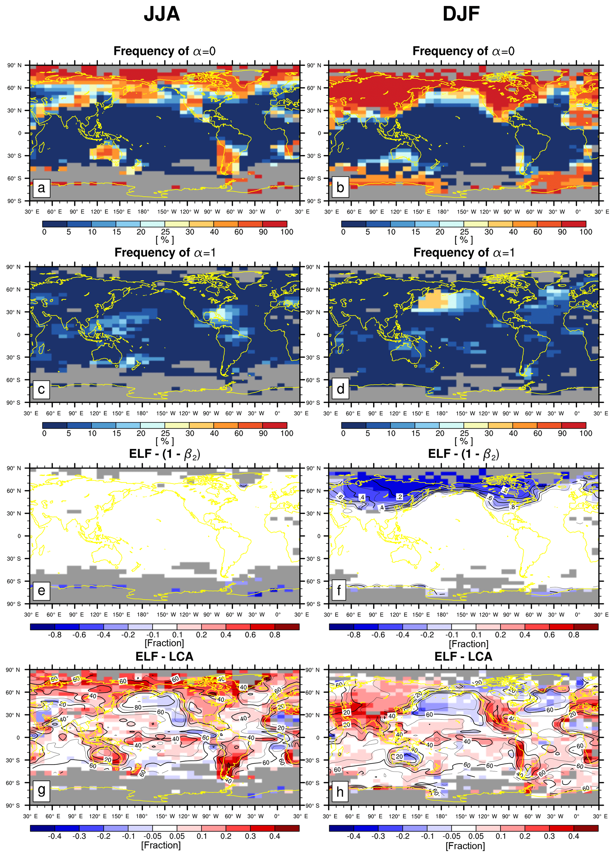
Figure 2(a, b) Frequency of occurrence of α=0 (i.e., zinv≤zLCL) among all observations (the sum of , α=0, and α=1); (c, d) frequency of occurrence of α=1 (i.e., ) among all observations; (e, f) the difference between ELF and , where f is the freeze-dry factor (see Eqs. 9, 10); and (g, h) the difference between ELF and LCA during (left column) JJA and (right column) DJF. In panels (e) and (f), the contour lines denotes the freeze-dry factor, f. In panels (g) and (h), the contour lines denotes the climatological LCA reported by surface observers. All observations are used for the panels (e)–(h). The grid boxes with a climatological observation number below 100 in each season are masked by gray color.
In reality, the key factor controlling the formation of clouds is the relative humidity. According to our conceptual framework, most of the clouds are likely to form at the inversion base. To compute the relative humidity at the inversion base, , we follow PLR04 and assume that the decoupling parameter, α, defined in Eq. (3) also describes the decoupling of the water vapor specific humidity, qv. Then, the water vapor specific humidity () and potential temperature () at the inversion base can be computed as and . The lapse rate of qv in the free atmosphere , which is required to compute , is obtained from the linear slope of qv at the 700 and 750 hPa levels. Using and , we compute as an additional proxy for LCA. We note that only needs the information on ; the other proxies do not need information on the vertical profile of qv other than qv,ML to compute zLCL.
2.2 Data and analysis
The surface observation data used in our study are from the Extended Edited Cloud Report Archive (EECRA, Hahn and Warren, 1999) for January 1956 to December 2008 over the ocean (without sea ice) and January 1971 to December 1996 over land. The EECRA compiles individual ship and land observations of clouds (e.g., cloud amount and cloud type for each low, middle, and upper level), present weather (e.g., fog, rain, snow, thunderstorm shower, and drizzle), and other coincident surface meteorologies (e.g., sea level pressure, sea surface temperature, ship-deck air temperature, dew-point depression, and wind speed and direction) at every 3 or 6 h based on the strict hierarchy of the World Meteorological Organization (WMO, WMO, 1975). Following Park and Leovy (2004), we filtered out the observations obtained under poor illumination conditions (i.e., the moonlight screening criteria, Hahn et al., 1995), from the WMO's Historical Sea Surface Temperature (HSST) Data Project (identified by card deck numbers 150–156), or with any missing surface meteorologies or cloud information. In this study, we focus on the analysis of LCA of all cloud types including cumulus as well as stratus. The upper-level meteorologies (e.g., p, θ, and qv) are from the ERA-Interim reanalysis products (ERAI, Simmons et al., 2007) from January 1979 to December 2008 at 6-hourly time intervals. Spatial and temporal interpolations are performed to compute the upper-level meteorologies at the exact time and location at which the EECRA surface observers reported LCA. Because both EECRA and ERAI are necessary, our analysis only uses the data from January 1979 to December 2008 (30 years) over the ocean and January 1979 to December 1996 over land (18 years). Using the 6-hourly ERAI vertical profiles of θ and qv interpolated to individual EECRA surface observations, we computed the 12 proxies for LCA (LTS, EIS, ECTEI, IS, DS, α, zLCL, zinv, , β1, β2, ELF) and averaged them into 5∘ latitude × 10∘ longitude seasonal data for each year. Thus, if there is no missing grid value, a total of 120 and 72 seasonal datapoints is available in each grid box over the ocean and land, respectively. To reduce the impact of random noise in association with the small observation number, the year with an observation number smaller than 10 in each season and grid box is not used in our analysis.
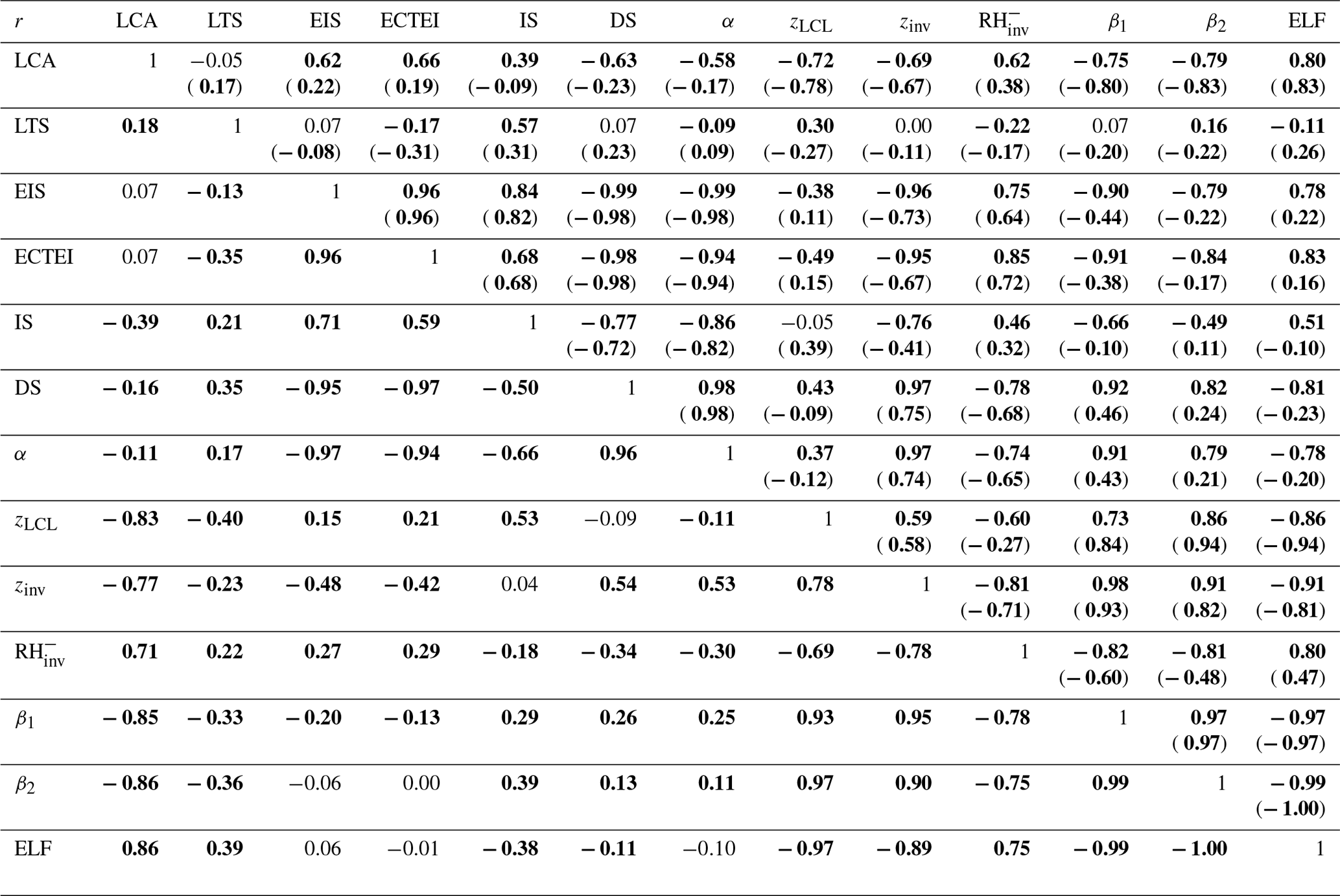
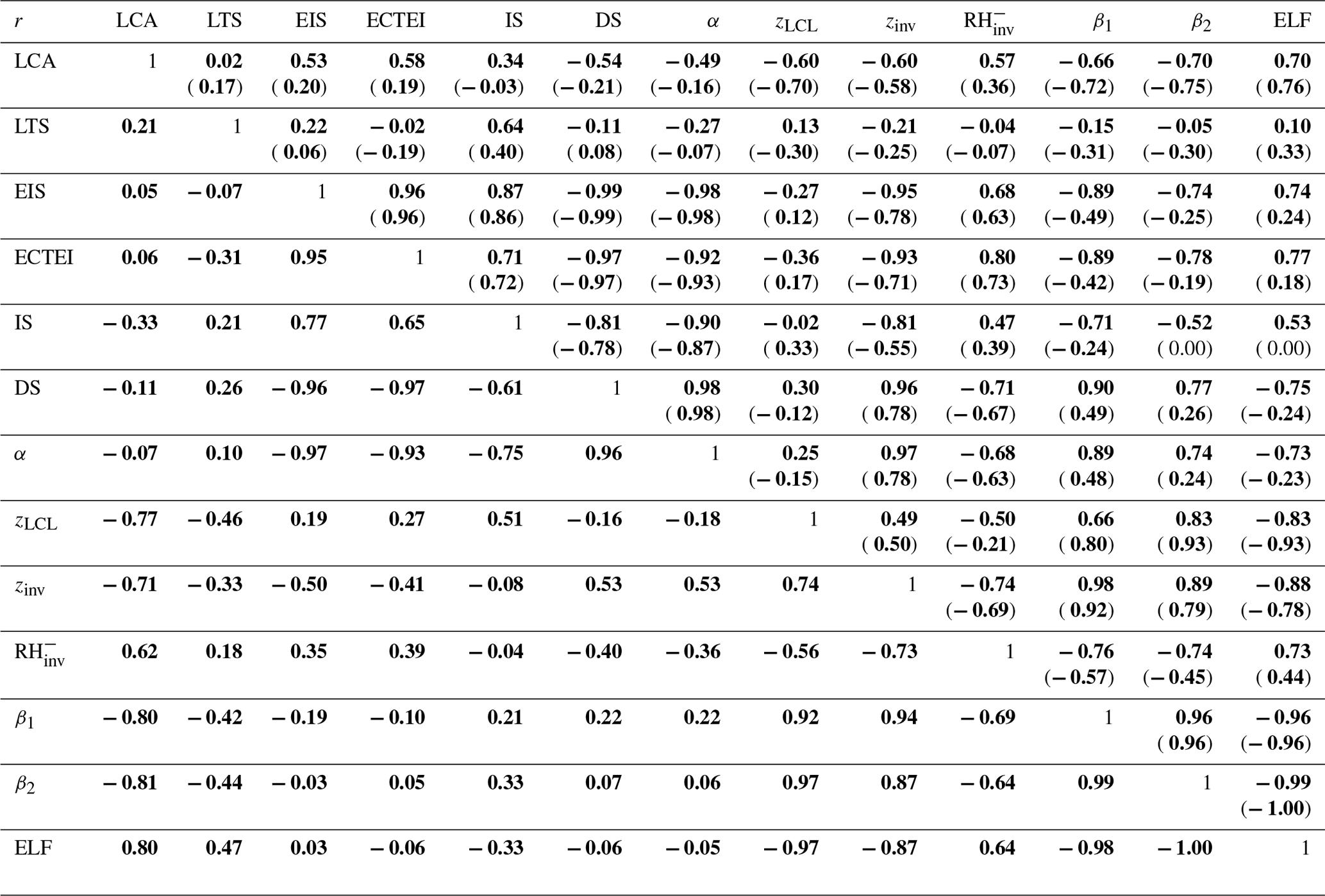
Table 1Spatial–seasonal correlation coefficients between LCA and various proxies for the climatological seasonal data (DJF, MAM, JJA, SON) of each 5∘ latitude × 10∘ longitude grid box (values in the upper right: over the ocean; values in the lower left: over land; and values within the parenthesis: over the entire globe including the coast). Statistically significant correlations at the 99.9 % confidence level from the Student t test assuming independent samples are denoted by the bold characters. The same convention is applied to the following tables. Only the data satisfying are used for this table.
Three separate correlation analyses were performed between LCA and the 12 proxies: spatial–seasonal correlation analysis using climatological seasonal (i.e., DJF, MAM, JJA, SON) grid data (Table 1 and Figs. 3–6; Table 4 and Figs. 11, 12) or climatological seasonal data averaged over selected regions (Figs. 7, 8, 12), seasonal–interannual and interannual correlation analysis using seasonal grid data from each year (Figs. 9–10, 13) or seasonal data averaged over selected regions from each year (Tables 2, 5), and combined spatial–seasonal–interannual correlation analysis (Tables 3, 6) using seasonal grid data over the globe in each year. For the spatial–seasonal correlation analysis, only the seasons and grid boxes with a climatological seasonal observation number equal to or larger than 100 are used. For any temporal correlation analysis containing interannual variations, we only used the years and seasons with a seasonal observation number equal to or larger than 10 for each year within the grid box or selected regions. Only the grid boxes with the number of effective seasonal data points equal to or larger than 50 out of the maximum 120 over the ocean (30 years) and 72 over land (18 years) are used for the temporal correlation analysis.
As the reference height near the surface, we tested both pref=p1000 and pref=psfc. In both cases, the density of the atmosphere within the lower troposphere below 700 hPa was set to ρ=1 kg m−3. When pref=p1000, all thermodynamic properties at p1000 (e.g., p, θ, and qv) are obtained from 6-hourly ERA-Interim data interpolated into the time and location of individual EECRA observations. The geometric height of p1000 from the surface (z1000) is computed using a hydrostatic equation. If the air at p1000 is saturated, zLCL is set to z1000. When pref=psfc, a set of thermodynamic properties at psfc (e.g., θ, qv) is obtained from two different data sources: one is from the 6-hourly ERA-Interim data interpolated into the time and location of individual EECRA observations similar to the case of pref=p1000 and the other is from EECRA surface observations. When the surface air is saturated, we set zLCL=zsfc. Three separate analyses were performed using individual datasets (e.g., pref=p1000, pref=psfc with ERA-Interim surface data, and pref=psfc with EECRA surface observations). In the next section, we will show the results based on pref=psfc with EECRA surface observations of psfc, θsfc, and qv,sfc. The analyses using the other two choices produced similar results. It is not shown here, but the same analysis using the NCEP/NCAR reanalysis product (Kalnay et al., 1996) instead of the ERA-Interim data also produced similar results.
A fundamental assumption of our decoupling hypothesis is that thermodynamic scalars at the inversion base () are bounded by the ML (θML) and inversion top () properties. That is, the decoupling parameter α is between 0 and 1 (see Eq. 3). However, the inversion height, zinv, estimated from Eq. (4) can have any numerical values, such that α parameterized by zinv (i.e., ) can be smaller than 0 or larger than 1. To be consistent with our decoupling hypothesis, we reset zinv=zML whenever zinv estimated from Eq. (4) is smaller than zML (i.e., we wrap all α<0 to α=0), and, similarly, we reset whenever the estimated zinv is larger than Δzs+zML (i.e., we wrap all α>1 to α=1). As shown in Fig. 2, the cases of α=0 after wrapping frequently occur in stably stratified regimes over the Arctic and northern continents in winter, desserts during the night, the northwestern Pacific and southern-hemispheric (SH) circumpolar regions during boreal summer when warm air is advected into cold SST, and along the west coast of major continents where cold SST exists due to coastal upwelling. On the other hand, the cases of α=1 after wrapping occur in unstable regimes over the tropical SST warm pools in JJA and along the midlatitude storm tracks during winter. In the next section, we will first present the results based on the data of and then all data of (e.g., the sum of , α=0, and α=1).
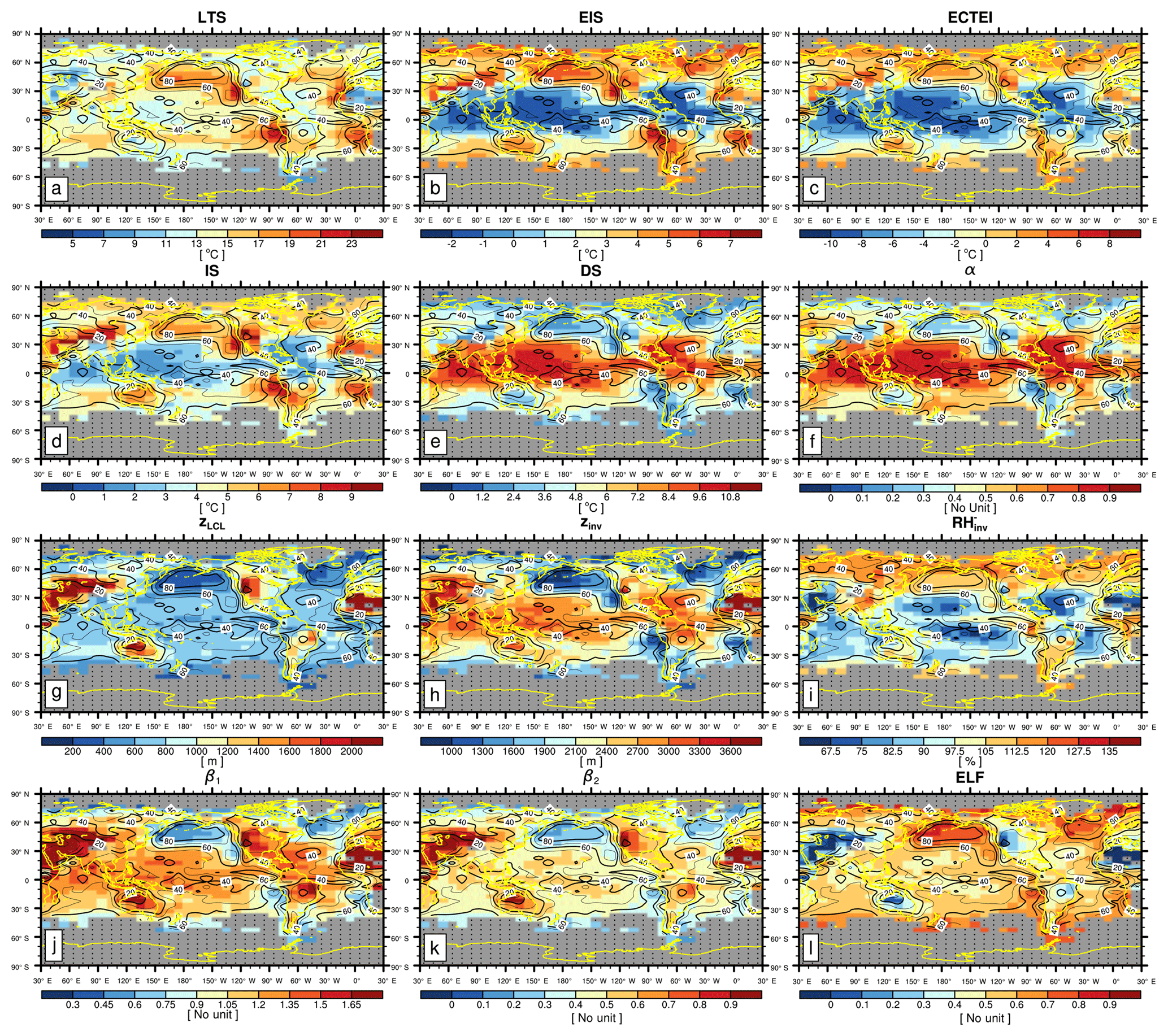
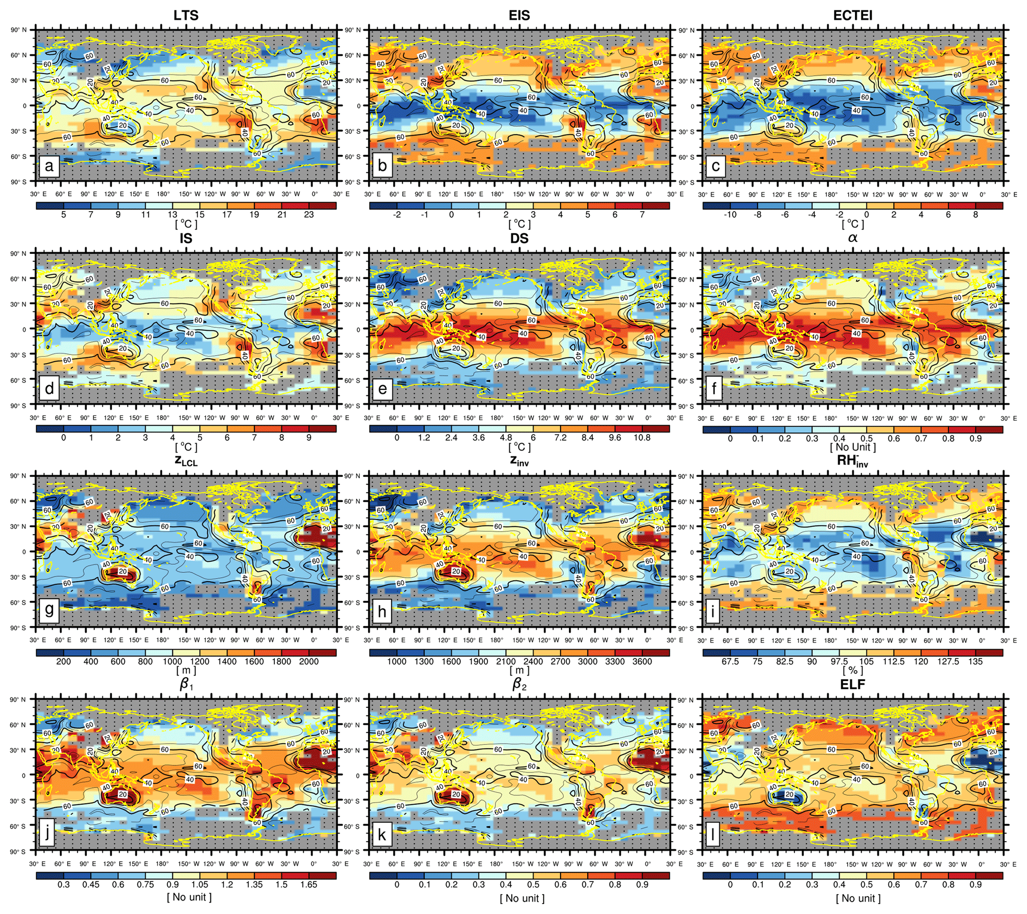
Figure 3Global distribution of climatological (a) lower-tropospheric stability (LTS), (b) estimated inversion strength (EIS), (c) estimated cloud-top entrainment index (ECTEI), (d) inversion strength (IS), (e) decoupling strength (DS), (f) decoupling parameter (α), (g) lifting condensation level of near-surface air (zLCL), (h) inversion height (zinv), (i) relative humidity at the inversion base (), (j) the first low-level cloud suppression parameter (β1), (k) the second low-level cloud suppression parameter (β2), and (l) estimated low-level cloud fraction (ELF) in June–July–August (JJA). The contour line denotes the climatological LCA in JJA reported by surface observers. The grid boxes with a climatological observation number below 100 in JJA are masked by gray color and dots. Only the data satisfying are used for this figure.
3.1 Spatial–seasonal correlation
Figures 3 and 4 show the seasonal climatology of LCA (solid lines; also see Fig. 7 for the color maps of LCA in the 2.5∘ latitude × 5∘ longitude grid box) and 12 proxies for LCA defined in the previous section during JJA and DJF, respectively. The spatial–seasonal correlation coefficients between these variables are summarized in Table 1. The scatter plots between the 12 proxies and LCA over the ocean and land are shown in Figs. 5 and 6, respectively.
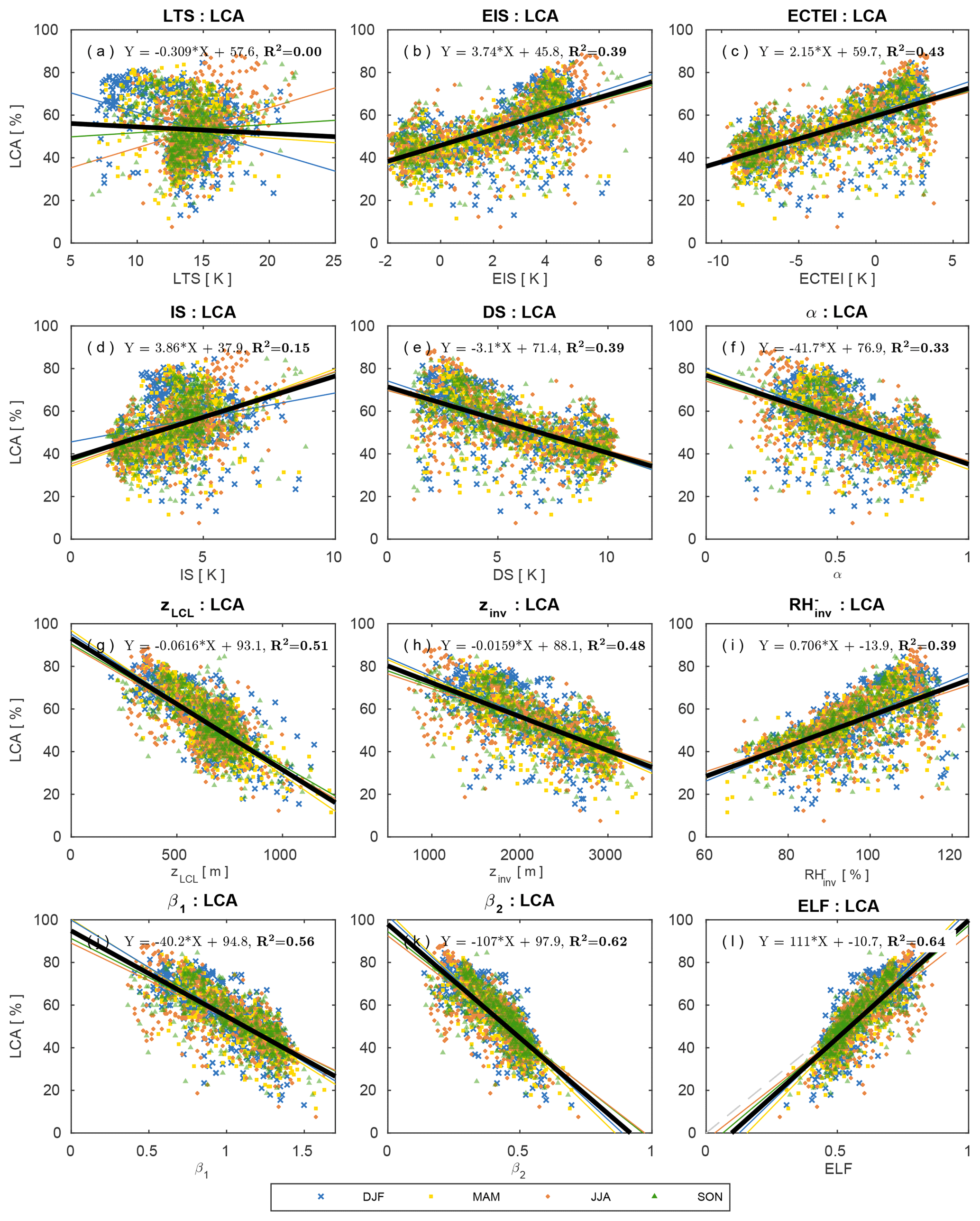
Figure 5Scatter plots between LCA and various proxies over the ocean. Each dot reflects climatological seasonal data at each 5∘ latitude × 10∘ longitude grid box shown in Figs. 3 and 4, and different colors denote different seasons. Also plotted are the least-squares fitting lines for each season (colored lines) and all seasons (thick black line) and regression equations for all seasons with the corresponding fraction of variance (R2) explained by the all-seasons regression equation. The dashed gray line in (l) denotes LCA=ELF. Only the data satisfying are used for this figure.
Consistent with KH93 and WB06, both LTS and EIS are strong in subtropical marine stratocumulus decks west of major continents but weak in the tropical deep convection regime in which LCA is small. Although the overall pattern of EIS looks similar to that of LTS, several notable differences exist between them. For example, in the vicinity of polar and high-latitude regions in both hemispheres where LCA is large, EIS is strong but LTS is weak, which seems to contribute to a low spatial–seasonal correlation between LTS and EIS over the globe (see Table 1). According to Eq. (2), EIS here should be weaker than in other regions, because zLCL is low in these cold regions (see Figs. 3g and 4g). However, probably due to the decreases in and z700 in the cold region, EIS becomes strong here, resulting in a better spatial–seasonal correlation between EIS and LCA (r=0.62) than between LTS and LCA () over the ocean. Table 1 shows that the spatial–seasonal correlation between LTS and LCA is very weak over the ocean and land. This is somewhat surprising, because KH93 reported that LTS is significantly positively correlated with LCA. It should be noted that KH93's finding was based on the analysis over the marine stratocumulus deck, while our result is based on global analysis. Because of this potential sensitivity of the relationship between LTS and LCA to the analysis domain, we need to be careful when using LTS as a global proxy for LCA in climate sensitivity studies.
The spatial pattern of the inversion strength (IS, Figs. 3d and 4d), which is about 1–3 K higher than EIS, is roughly similar to that of EIS. However, in contrast to EIS but similar to LTS, IS tends to be small in high-latitude regions, which results in a weaker spatial–seasonal correlation between IS and LCA over the ocean (r=0.39) than between EIS and LCA. Table 1 shows that the decoupling strength (DS, Figs. 3e and 4e) is almost perfectly correlated with EIS over the globe (), with a correlation with LCA very similar to that of EIS. However, the named EIS has a weaker correlation with inversion strength than anti-correlation with decoupling strength. In other words, a strong EIS indicates that the air at the inversion base is coupled well with the surface-based ML air. The decoupling parameter (α, Figs. 3f and 4f) also has a near-perfect correlation with EIS (), supporting our interpretation of EIS. When , it becomes . As will be shown later, stronger correlation among EIS–DS–α than EIS–IS also exists in the combined spatial–seasonal–interannual correlation statistics (Table 3) and in the analysis using all of the observation data (Tables 4 and 6).
The inversion height (, Figs. 3h and 4h), which is strongly correlated with EIS, DS, and α, has a high spatial–seasonal correlation with LCA ( over the ocean and over land), even better than EIS (r=0.62 over the ocean and r=0.07 over land). The superiority of zinv over EIS as a proxy for LCA is more pronounced over land. Why does zinv characterize LCA better than EIS over land? If , such that the different correlation characteristics of zinv and EIS with LCA are likely associated with zLCL. In the case that surface air is saturated and very low-level clouds are formed (e.g., fog with a low zLCL), small zLCL causes EIS to decrease ( from Eq. 2). This contributes to the weaker, negative EIS–LCA correlation seen over land compared to the stronger, positive correlation observed in the marine stratocumulus deck. Because zinv is defined as the addition of zLCL to EIS, the undesirable negative impact of zLCL to the correlation with LCA is removed from EIS compared to zinv. Over the western continental United States during summer, both zLCL and zinv are at their maximum where LCA is at its minimum. In this region, similar to the ocean case, zinv is negatively correlated with LCA; however, opposite to the ocean case, EIS is not positively correlated with LCA. Consequently, EIS has a weaker global spatial–seasonal correlation with LCA (r=0.22) than zinv (). It is very interesting to note that a simple proxy, zLCL, shows a stronger spatial–seasonal (and also spatial–seasonal–interannual) correlation with LCA than LTS, EIS, and zinv over both the ocean and land.
According to our conceptual framework, low-level clouds likely form just below zinv (see Fig. 1). If that is the case, it is likely that the relative humidity at the base of zinv () is a good proxy for LCA. Over both the ocean and land, shows a stronger correlation with LCA than LTS and EIS but a weaker correlation than zinv and zLCL. We speculate that this relatively poor performance of compared to zinv and zLCL is due in part to the poor estimation of rather than indicating that is a poor proxy for LCA. Because is estimated using the roughly estimated and without performing any saturation adjustment, the absolute values of in our analysis can be unreasonably larger than 100 % in some regions (Figs. 3i and 4i).
The spatial patterns of two LCS parameters, and , are roughly similar to those of zinv and zLCL. However, both LCS parameters have a better spatial–seasonal correlation with LCA than zinv and zLCL, with β2 showing a slightly better performance than β1 (see Table 1 and Figs. 5, 6). The estimated low-level cloud fraction, , shows a very similar correlation to β2 because the freeze-dry factor, f, is approximately 1 in the regime of (see Fig. 2). Among all 12 proxies, β2 and ELF have the highest spatial–seasonal correlation with LCA over both the ocean and land. ECTEI is equivalent if slightly better than EIS for the ocean, equivalent over land, and between LTS and EIS over the globe.
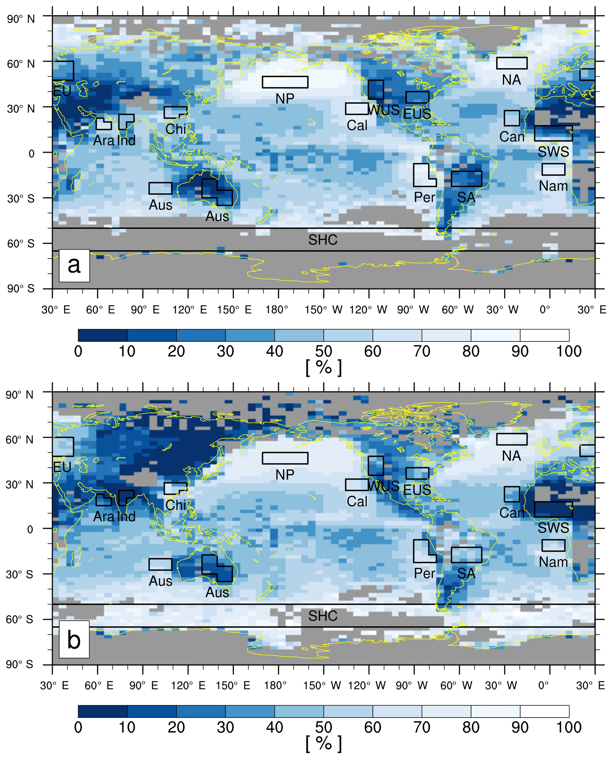
Figure 7The seasonal climatology of LCA during (a) JJA and (b) DJF in the 2.5∘ latitude × 5∘ longitude grid box. The grid boxes with a climatological observation number below 25 in each season are masked by gray color. The domains selected for computing temporal (seasonal–interannual and interannual only) correlation coefficients in Tables 2 and 5 are also plotted: Peruvian (7.5–22.5∘ S, 80–90∘ W and 17.5–22.5∘ S, 75–80∘ W), Namibian (7.5–15∘ S, 5∘ W–10∘ E), Californian (25–32.5∘ N, 120–135∘ W), Australian (20–27.5∘ S, 95–110∘ E), Canarian (17.5–27.5∘ N, 20–30∘ W), Arabian (15–20∘ N, 60–70∘ E and 20–22.5∘ N, 60–65∘ E), North Pacific (42.5–50∘ N, 170–200∘ E), North Atlantic (55–62.5∘ N, 15–35∘ W), southern-hemispheric circumpolar region (50–65∘ S, 0–360∘ E), China (25–30∘ N, 105–120∘ E and 22.5–25∘ N, 105–115∘ E), India (20–25∘ N, 75–85∘ E and 15–20∘ N, 75–80∘ E), Europe (47.5–60∘ N, 30–45∘ E and 47.5–55∘ N, 20–30∘ E), eastern US (32.5–40∘ N, 80–95∘ W), western US (35–47.5∘ N, 110–120∘ W), South America (12.5–22.5∘ S, 45–65∘ W), Australia (25–35∘ S, 140–150∘ E and 17.5–30∘ S, 130–140∘ E), and southwestern Sahara (7.5–17.5∘ N, 10∘ W–15∘ E).
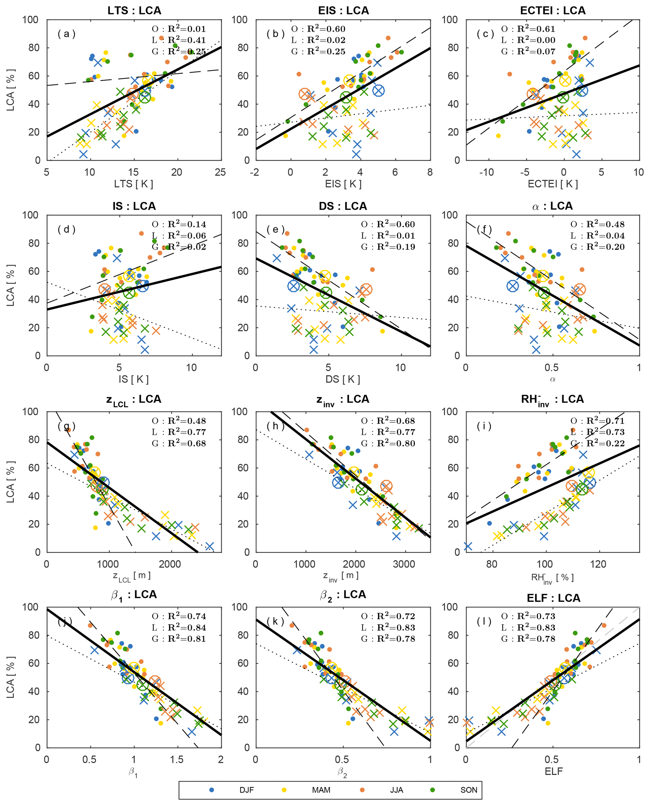
Figure 8Scatter plots between the seasonal LCA and various proxies over selected regions of Fig. 7. Different colors denote different seasons. The ocean and land regions are denoted by dots and “x” marks, respectively, except for the China stratocumulus deck, which is denoted by the circled “x” marks. Also plotted are the least-squares fitting lines for ocean (O; dashed line), land (L; dotted line), and globe (G; thick solid line), respectively, with the fraction of variance (R2) explained by the regression lines. Only the data satisfying are used for this figure.
Figure 8 shows the scatter plots between the seasonal LCA and 12 proxies in several regions shown in Fig. 7. LTS over land shows a stronger interregional–seasonal correlation with LCA than that over the ocean; however, EIS (and ECTEI, DS, and α) over the ocean has a stronger correlation than that over land. Over both the ocean and land, zinv and zLCL are strongly correlated with LCA. is strongly correlated with LCA over the ocean and land; however, the correlation over the globe is weak. Each of β1 and β2–ELF explains about 80 % of the interregional–seasonal variations of the seasonal LCA, which is a much larger percentage than those explained by LTS (25 %), EIS (25 %), and ECTEI (7 %). Except LTS, the difference between the regression slopes for the ocean and land in each proxy shown in Fig. 8 is generally larger than the seasonal differences between the regression slopes shown in Figs. 5 and 6, indicating a need to incorporate additional factors characterizing the contrast between the ocean and land in the future.
3.2 Seasonal–interannual correlation
Figure 9 shows the global distribution of seasonal–interannual correlation coefficients between the seasonal LCA and 12 proxies. Over the North Pacific and subtropical marine stratocumulus deck west of major continents, LTS and LCA are positively correlated. However, a negative correlation also exists, for example, over Europe and the northwestern Atlantic. Similar to LTS, EIS and LCA are positively correlated over marine stratocumulus deck; but interestingly, the correlation signs over the northwestern Atlantic and Europe and several continents (e.g., Southeast Asia, Australia, South America, and Central Africa) are reversed compared with LTS. As mentioned before, zLCL mainly contributes to the different correlation characteristics between EIS and LTS with LCA in these regions (see Eq. 2). Although LTS and EIS are good proxies for LCA over the marine stratocumulus deck, they have a limitation as a global proxy due to the spatial changes of temporal correlation signs. ECTEI shows very similar correlation characteristics to EIS. With an opposite sign, the overall correlation patterns of DS and α are quite similar to that of EIS. Compared with the other proxies, LCA tends to be more homogeneously correlated with zLCL, zinv, , β1, and β2 and ELF over the globe, without the spatial reversal of the correlation sign. Figure 10 shows a similar temporal correlation analysis to that shown in Fig. 9 but only for interannual variations without the seasonal cycle. Overall, the spatial pattern of interannual correlation is similar to that of seasonal–interannual correlation; however, the magnitude is reduced, particularly over the marine stratocumulus deck. Both in terms of seasonal–interannual and interannual correlations, β2 and ELF perform better than LTS and EIS over the entire globe without the spatial changes of temporal correlation signs; thus, they are well suited as global proxies for LCA. β1 performs nearly as well if not equivalently to β2 and ELF.

Figure 9Global distribution of temporal (seasonal plus interannual) correlation coefficients between the seasonal LCA and various proxies: (a) LTS, (b) EIS, (c) ECTEI, (d) IS, (e) DS, (f) α, (g) zLCL, (h) zinv, (i) , (j) β1, (k) β2, and (l) ELF. The contour line denotes the climatological annual LCA reported by surface observers, and the grid boxes with a climatological annual observation number below 100 are denoted by dots. Only the grid boxes with the number of effective seasonal data used for the correlation analysis equal to or larger than 50 out of the maximum 120 over the ocean and 72 over land are plotted. The grid boxes that are not satisfying these conditions are masked by dark gray color. The minimum magnitudes of correlation coefficients statistically significant at the 99.9 % confidence level with the numbers of independent samples of 120 (ocean max), 72 (land max), and 50 (minimum requirement) are 0.3, 0.38, and 0.45, respectively. Only the data satisfying are used for this figure.
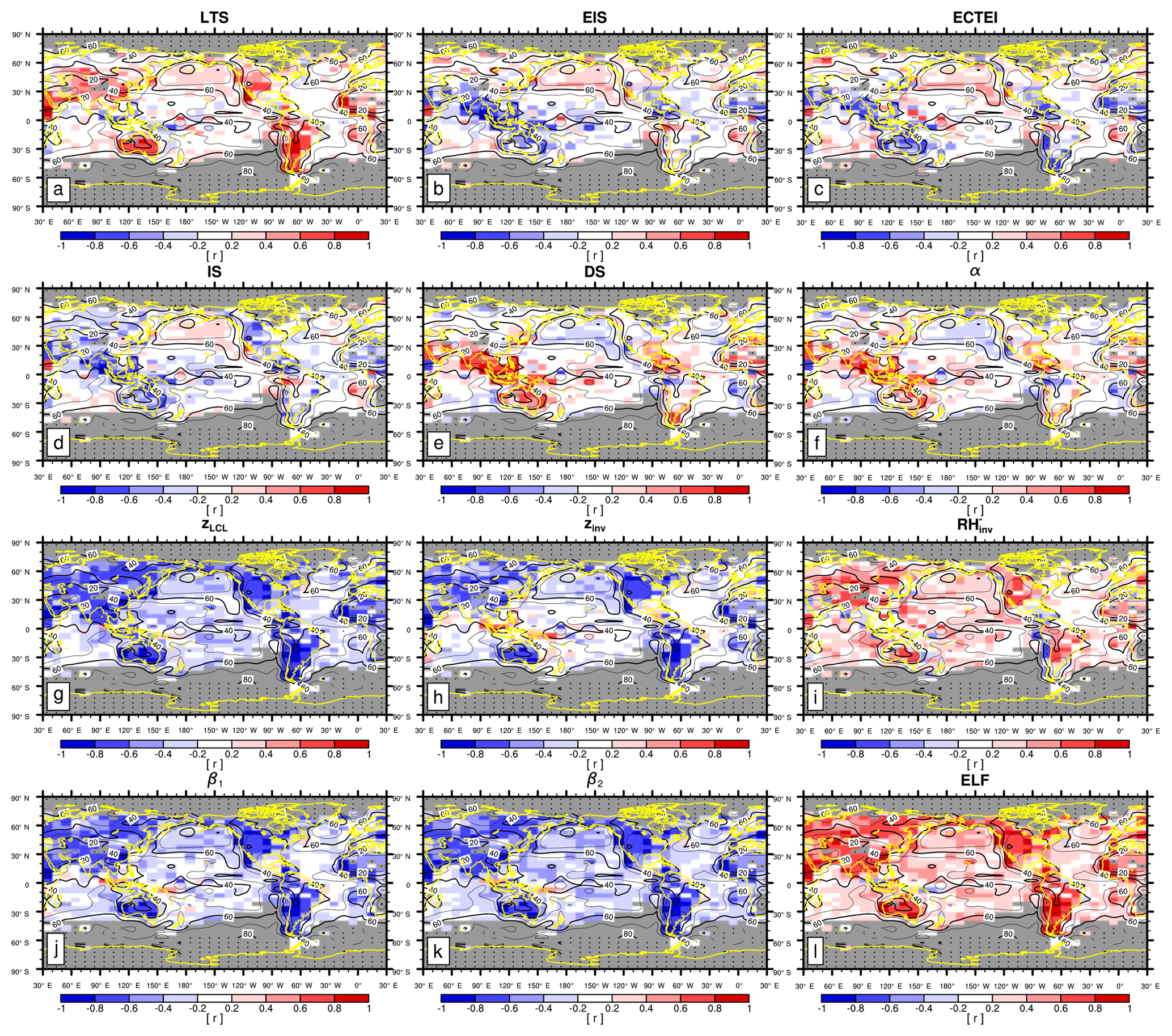
Figure 10The same as Fig. 9 but for interannual variation only without the seasonal cycle. This plot was generated by using the four-seasons data (DJF, MAM, JJA, SON) in each year with the seasonal climatology subtracted in each season, such that only interannual variation is included in this correlation analysis.
Table 2Temporal (rs+i: seasonal plus interannual, ri: interannual only) correlation coefficients of the seasonal LCA fitted to the individual proxy for selected regions shown in Fig. 7. Only the data satisfying are used for this table.
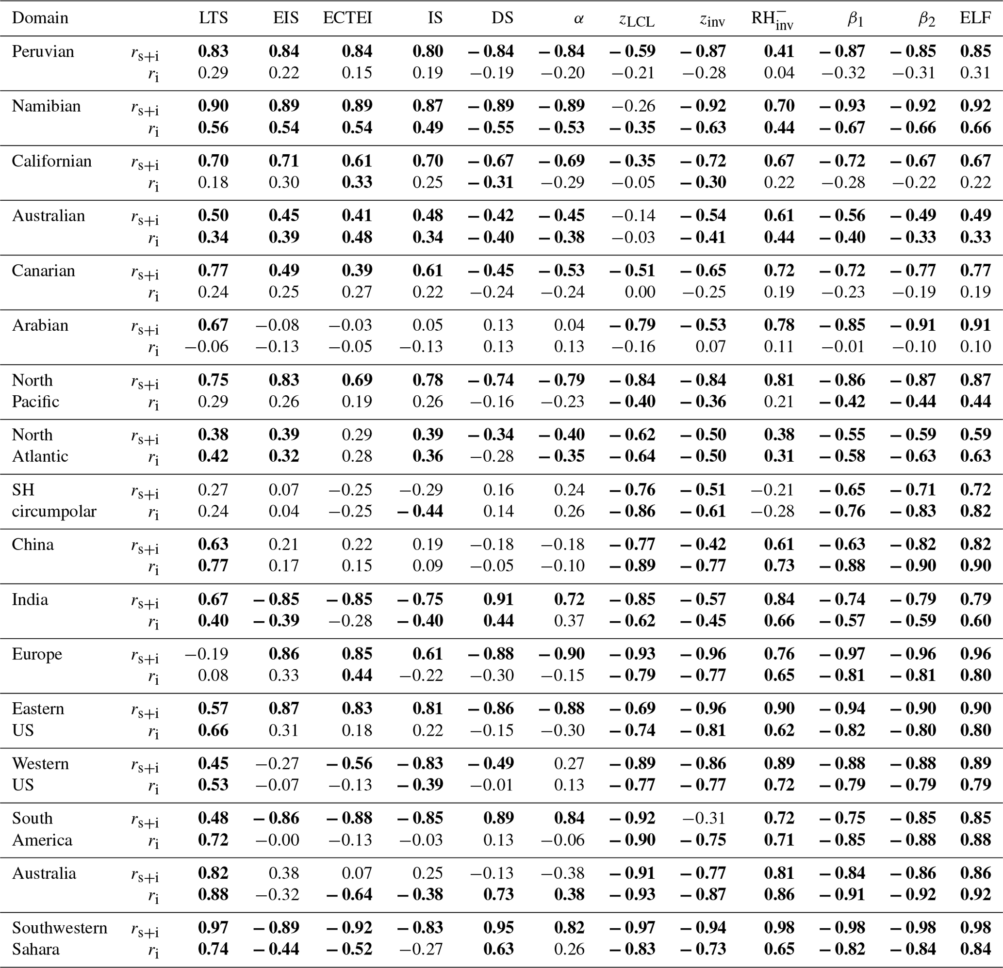
Table 2 summarizes the temporal correlation coefficients between LCA and 12 proxies for various regions shown in Fig. 7. The first six regions in our analysis are the subtropical marine stratocumulus decks. Although less well known than the other regions, stratocumulus and fog also exist over the Arabian Sea during summer and thus are included in our analysis (see Park and Leovy, 2004; Schubert et al., 1979; and also Fig. 7a). The next three regions are the midlatitude marine stratocumulus decks which have large LCA and undergo frequent passages of synoptic storms (North Pacific, North Atlantic, SH circumpolar). The last seven regions are over the continents and have small LCA. China is a unique continental stratocumulus deck with high LCA. Over the marine stratocumulus decks, except in the SH circumpolar region, LTS has a significant positive seasonal–interannual correlation with LCA. In all regions except the Arabian Sea, both EIS and ECTEI show strong correlations similar to that of LTS. Although mainly designed as a proxy for the marine stratocumulus fraction, LTS is also positively correlated with some continental LCA in a statistically significant way. On the other hand, as is also shown in Fig. 9, EIS and ECTEI are strongly negatively correlated with the continental LCA over India, South America, and the southwestern Sahara. Similar to the spatial–seasonal correlations, the temporal correlation characteristics of DS and α with LCA are very similar to that of EIS. Over the stratocumulus decks, zinv is a proxy that is as good as or better than LTS and EIS. Notably, zLCL shows a very good performance over land (and also in the midlatitude marine stratocumulus decks), indicating that surface moisture (regardless of whether it is locally originated or advected) substantially contributes to the temporal variations of the continental LCA. In most areas, has a significant positive seasonal–interannual correlation with LCA. In general, the interannual correlation tends to be weaker than the seasonal–interannual correlation. In the subtropical marine stratocumulus decks, except the Namibian and Australian ones, the seasonal cycle dominantly contributes to the temporal correlation between various proxies and LCA. Regardless of whether the seasonal cycle is included or not, two LCS parameters (β1,β2) and ELF have better temporal correlations with LCA than any other proxies over almost all regions, including the marine stratocumulus decks.
Table 3 summarizes the combined spatial–seasonal–interannual correlations between the seasonal LCA and 12 proxies. Over the ocean, EIS and ECTEI show better correlations with LCA than LTS. EIS correlates better with DS and α than with IS. As a global proxy for LCA, both zLCL and zinv perform better than LTS, EIS, and ECTEI because of their better performance over land. A very simple proxy, zLCL performs better than zinv and explains almost 50 % of the spatiotemporal variations of LCA over the globe. Among all 12 proxies, β2 and ELF explain the largest fraction of spatial and temporal variations of the seasonal LCA (more than 56 % over the entire globe), much more than the ones explained by LTS (3 %) and EIS (4 %). Over the ocean, β2 performs slightly better than β1 with a similar performance over land.
Table 3Combined spatial–seasonal–interannual correlation coefficients of the seasonal LCA fitted to the individual proxy with the same convention as Table 1. All seasonal data (DJF, MAM, JJA, SON) in each year in each 5∘ latitude × 10∘ longitude grid box are used. Only the data satisfying are used for this table.
3.3 Extended analysis using all data
Until now, we have presented results based on the analysis of the data satisfying (i.e., ) when our decoupling hypothesis can be applied without any conceptual ambiguity. However, for a fair comparison with the previous proxies of LTS, EIS, and ECTEI, which can be defined in any of the cases, it is necessary to examine the performance of various proxies in general situations. This section provides an extended analysis using all observation data of (i.e., the sum of , α=0, and α=1). Figure 2 shows the frequency of occurrence of α=0 and α=1 among all observations during JJA and DJF. The cases of α=0 frequently occur when the lower troposphere is highly stable (i.e., zinv≤zLCL) in the vicinity of the Arctic area north of 60∘ N, the northern continents and desserts during boreal winter, the northwestern Pacific and SH circumpolar regions during boreal summer, and along the west coast of major continents. On the other hand, the cases of α=1 occur when the troposphere is highly unstable (i.e., ) in the tropical warm pool regions during JJA and the midlatitude storm tracks during boreal winter. The differences between the results presented in this section and previous sections are due to the inclusion of the data obtained from these highly stable (α=0) and unstable regimes (α=1), mostly from stable regimes. This comparison allows us to obtain insights into the impact of extreme vertical stratification in the lower troposphere on the relationship between various proxies and LCA.
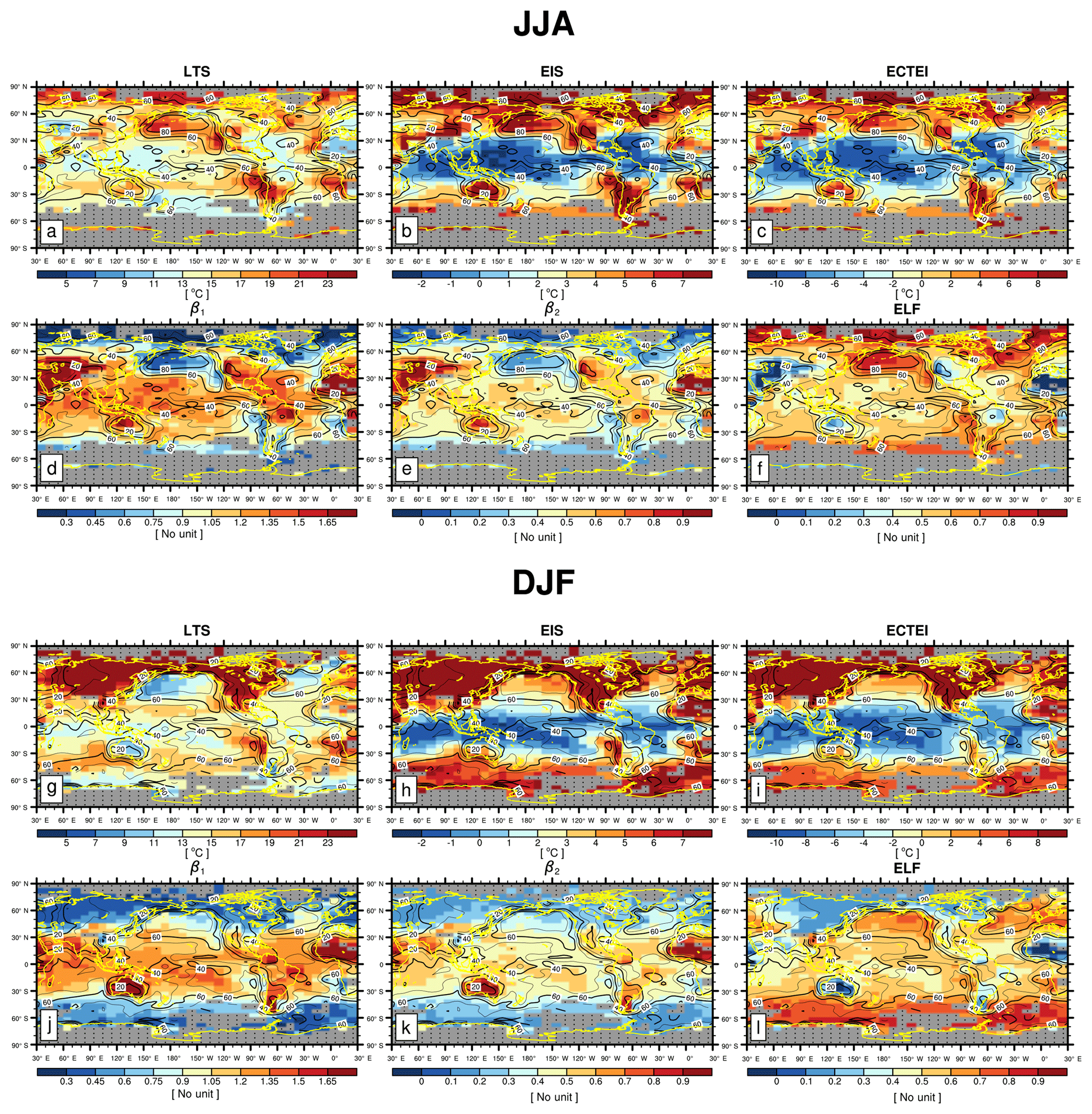
Figure 11Global distribution of climatological LTS, EIS, ECTEI, β1, β2, and ELF during JJA (upper) and DJF (lower), respectively. The contour line denotes the climatological seasonal LCA reported by surface observers. These figures are the same as Figs. 3 and 4 but were obtained from the analysis of all observation data (i.e., , α=0, and α=1).
Figure 11 shows the seasonal climatology of LCA (solid lines) and six key proxies (LTS, EIS, ECTEI, β1, β2, and ELF) during JJA and DJF, respectively, for all observation data. The overall pattern of the climatological proxies is similar to those with (Figs. 3, 4), but the magnitude in the high-latitude regions is amplified due mainly to the contribution of the data in the very stable regimes. In particular, over the northern continents during DJF, the values of LTS, EIS, and ECTEI (β1/β2) are substantially higher (lower) than those of . The spatial–seasonal correlation between LTS and EIS (r=0.85 in Table 4) is now much stronger than the previous case of ( in Table 1), but, in contrast to EIS, LTS still tends to decrease with latitude in the SH high-latitude regions.
Table 4The same as Table 1, but all data (i.e., and α=0 and α=1) are used for this table.
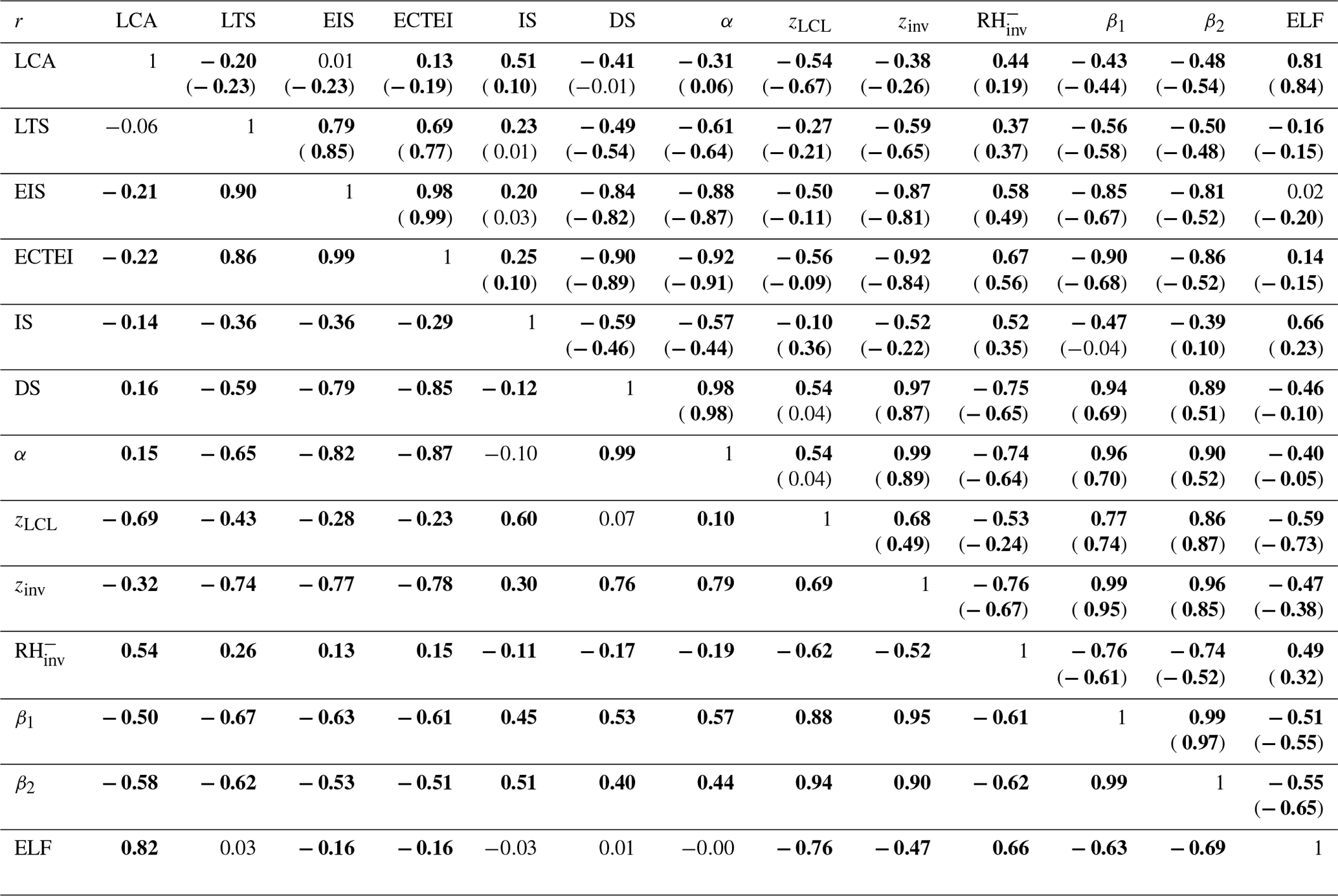
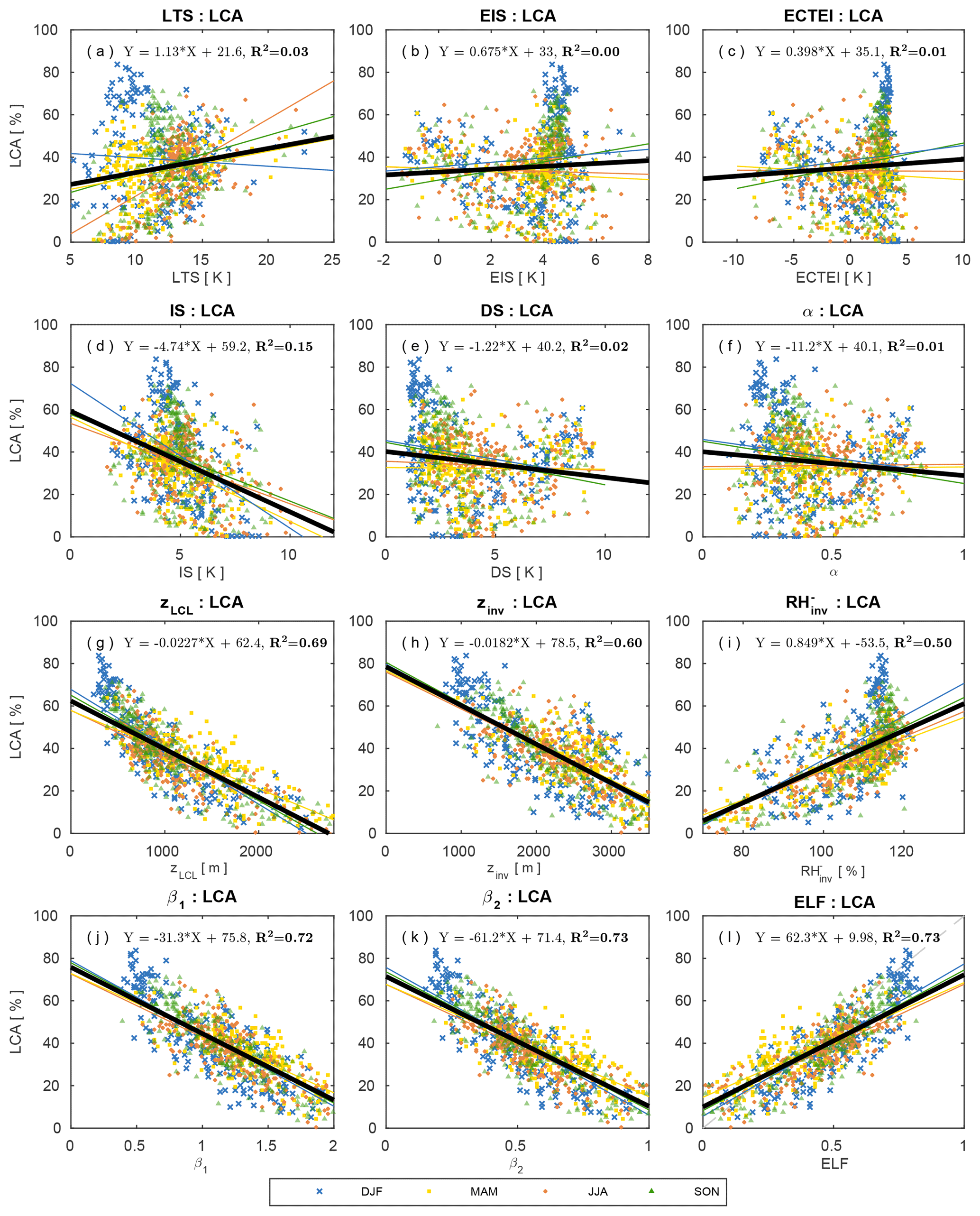
Figure 12 shows the scatter plots between LCA and six key proxies over the ocean, land, globe, and several regions defined in Fig. 7. This is the reproduction of Figs. 5, 6, and 8 using all observation data. Except ELF, the correlations between various proxies and LCA are degraded by the inclusion of the data from the very stable and unstable regimes. In particular, EIS and ECTEI over the ocean and two LCS parameters (β1 and β2) show substantial degradation of the correlation with LCA, due mainly to the enhanced scatters induced by the data in the very stable regimes where LCA is small (the light-colored data points of in Fig. 12). Very surprisingly, however, ELF continues to maintain a strong correlation relationship with LCA over both the ocean and land, explaining 70 % of spatial–seasonal variations of LCA over the entire globe, which is a much larger percentage than those explained by β1 (19 %), β2 (30 %), LTS (5 %), EIS (6 %), and ECTEI (4 %). In comparison with the scatter plots of individual 5∘ latitude × 10∘ longitude grid point data, the scatter plots of the selected regions (the last column of Fig. 12) show weaker degradation of correlations because the selected regions are relatively free from the occurrence of α=0 and α=1 (compare Fig. 7 with Fig. 2a, b). If the analysis is performed with stratiform LCA only, EIS and ECTEI show better performance than the ones shown in Fig. 12 (see Supplement).
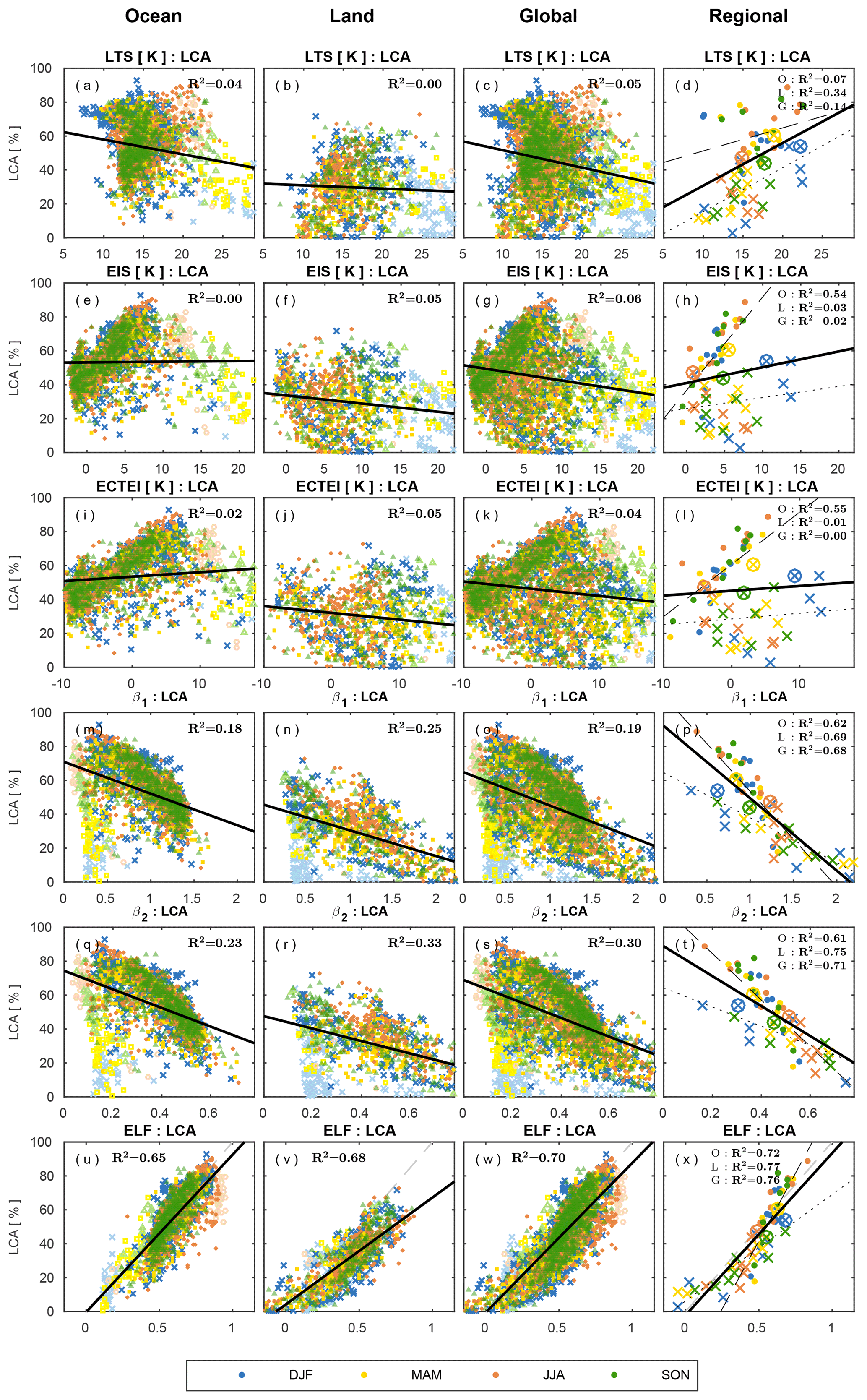
Figure 12Scatter plots between LCA and six proxies over the (first column) ocean, (second) land, (third) globe, and (fourth) selected regions shown in Fig. 7 with the least-squares fitting lines and the fraction of variance (R2) explained by the regression lines. The dashed gray line in the panels (u)–(x) denotes LCA=ELF. All observation data (i.e., , α=0, and α=1) are used for this figure. The grid data in the range of (i.e., very stable regime) are denoted by light colors in the first three columns.
Table 4 is the reproduction of Table 1 using all the data of , α=0, and α=1. Except the IS over the ocean and ELF, the correlations between the proxies and LCA are generally degraded in comparison to the previous case of . The spatial–seasonal correlations between LTS (and EIS, ECTEI) and LCA are very weak and even tend to be negative. Similar to the previous case, EIS is more strongly correlated with DS and α than with IS. Although it shows a weaker correlation than that in Table 1, zLCL still remains as a good proxy for LCA. Due mainly to the rapid decrease in the correlation between zinv and LCA, the correlations between two LCS parameters and LCA are substantially weaker than the previous case of . However, ELF successfully maintains a very strong spatial–seasonal correlation with LCA over both the ocean and land.
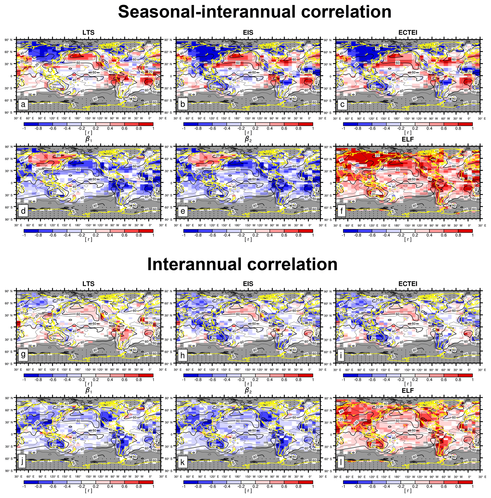
Figure 13Global distribution of seasonal–interannual (a–f) and interannual (g–l) correlation coefficients between the seasonal LCA and six key proxies (LTS, EIS, ECTEI, β1, β2, and ELF). The contour line denotes the climatological annual LCA reported by surface observers. These figures are the same as Figs. 9 and 10 but were obtained from the analysis of all observation data (i.e., , α=0, and α=1).
Figure 13 shows the global distribution of seasonal–interannual (upper) and interannual (lower) correlation coefficients between the seasonal LCA and six key proxies. The overall correlation patterns over the ocean are similar to the previous cases of (see Figs. 9 and 10). However, over Asia, LTS, EIS, and ECTEI show very strong negative seasonal–interannual correlations, resulting in the opposite correlations between the ocean and land. Over Asia, with similar contributions from zinv and zLCL (not shown but more strongly from zinv for seasonal–interannual and more strongly from zLCL for interannual correlations), both β1 and β2 show undesirable positive seasonal–interannual correlations with LCA. This indicates that LCS, similar to EIS, LTS, and ECTEI, is not appropriate as a global proxy for diagnosing seasonal–interannual variations of LCA. However, LCS is still a useful global proxy for diagnosing interannual variations of LCA. Among all the proxies examined, ELF remains the best proxy in terms of diagnosing both the seasonal–interannual and interannual variations of LCA over the globe, including the marine stratocumulus deck.
Table 5The same as Table 2, but all data (i.e., and α=0 and α=1) are used for this table.
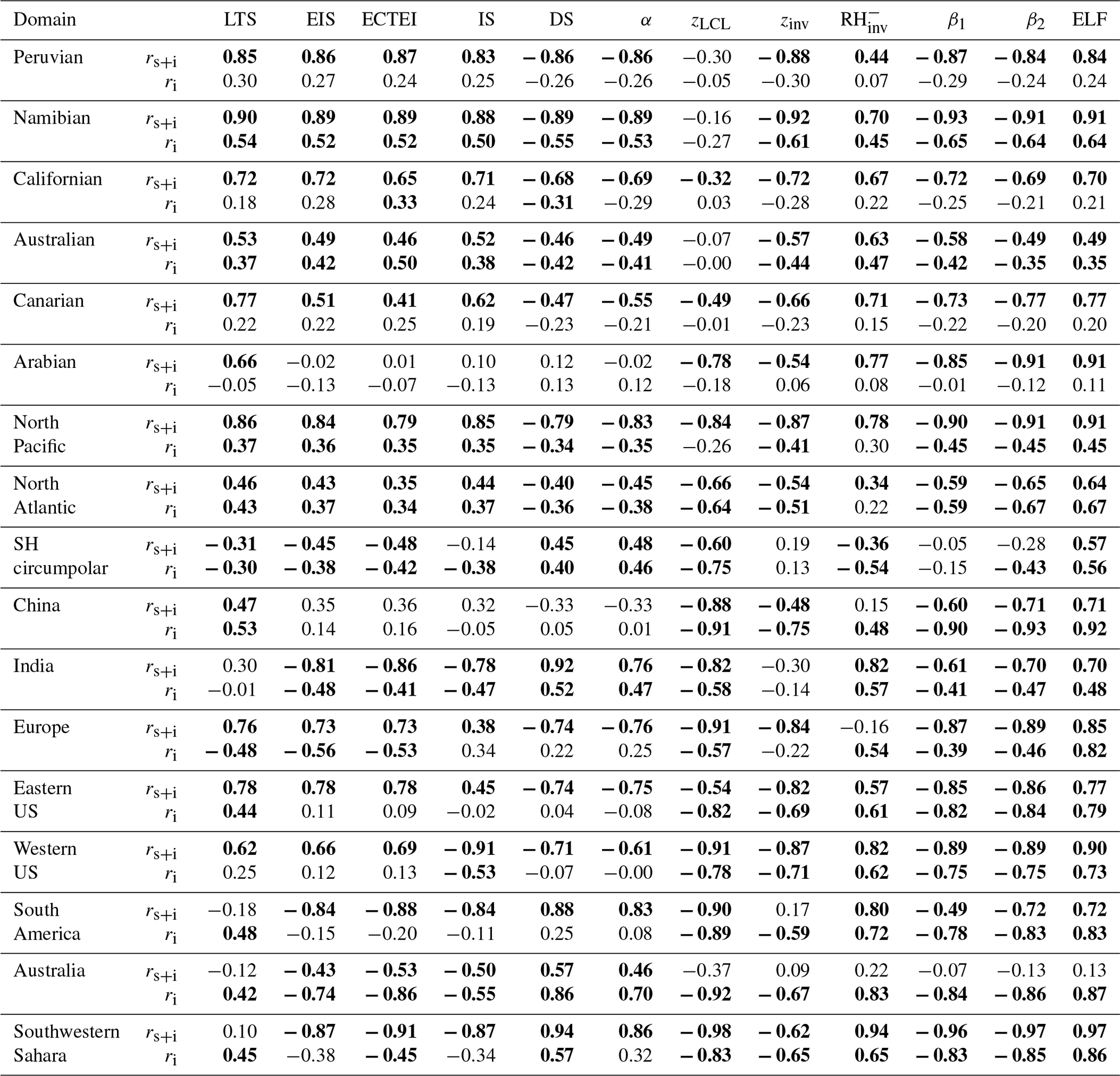
Table 5 is the reproduction of Table 2 using all data of . Similar to Table 2, LTS remains a good proxy for diagnosing the seasonal–interannual variations of LCA in the subtropical marine stratocumulus deck. However, its performance over several land areas (e.g., South America, Australia, southwestern Sahara, India, and China) is degraded, but its performance over Europe is improved. Both EIS and ECTEI show similar correlation characteristics to those in Table 2, but the undesirable negative correlation in the western US is changed to a desirable strong positive correlation. LTS outperforms EIS and ECTEI over the Arabian marine stratocumulus deck and India. LTS, EIS, and ECTEI all show undesirable significant negative correlations with LCA in the SH circumpolar region. In the stratocumulus deck (and also over most land areas), zinv remains as a proxy that is as good as or better than LTS and EIS. Over the land and midlatitude stratocumulus deck, including the Arabian region, zLCL tends to work better than zinv. Similar to Table 2, ELF and two LCS parameters perform better than LTS and EIS in most regions, including the marine stratocumulus deck. Overall, among the 12 proxies, ELF shows the best performance in diagnosing the seasonal–interannual variations of the seasonal LCA in a statistically significant way. The only exception is continental Australia in which both zLCL and zinv are weakly correlated with LCA. In addition to the combined seasonal–interannual variations, ELF also diagnoses the interannual variations of LCA well. However, similar to LTS and EIS, ELF still does not show good performance in diagnosing the interannual variations of LCA in several subtropical marine stratocumulus decks in a statistically significant way.
Table 6The same as Table 3, but all data (i.e., and α=0 and α=1) are used for this table.

Table 6 summarizes the combined spatial–seasonal–interannual correlations between the seasonal LCA and 12 proxies in general cases with all observation data. LTS is poorly correlated with LCA. Over the ocean, EIS and ECTEI show slightly better performance than LTS, but the improvement seems to be marginal. EIS correlates much better with DS and α than with IS. Among all 12 proxies, ELF shows the best performance in diagnosing the spatiotemporal variations of LCA, explaining almost 60 % of the spatial–seasonal–interannual variance of the seasonal LCA over the entire globe (50 % and 62 % over the ocean and land, respectively), which is a much larger percentage than those explained by LTS (2 %), EIS (4 %), and ECTEI (2 %).
Based on the decoupling parameterization of the cloud-topped PBL suggested by PLR04, a simple heuristic equation is derived to compute the inversion height, zinv. As an attempt to find a simple heuristic proxy for diagnosing the spatiotemporal variations of LCA over the globe, we defined two low-level cloud suppression parameters (LCS), and , by combining zinv with the lifting condensation level of near-surface air, zLCL, and normalizing with a constant scale height, Δzs=2750 m. To better diagnose LCA in extremely cold and dry atmospheric conditions, we also defined an estimated low-level cloud fraction, , with a freeze-dry factor, , where qv,ML is the water vapor specific humidity in the surfaced-based mixed layer that is assumed to be topped by zLCL, for simplicity. If zML≈zLCL where zML is the height of the surface-based mixed layer, then and , where the first factor in both formulae represents the degree of subsaturation of near-surface air, and the second factor represents the decoupling strength. ELF predicts that LCA increases as the inversion base air is thermodynamically coupled with the moist near-surface air containing enough water vapor. Considering that low-level clouds usually form at the inversion base, the conceptual cloud formation processes embedded in ELF are consistent with what is expected to happen in nature.
Using the near-surface θ and qv obtained from individual EECRA surface observations and the 6-hourly ERA-Interim profile of θ, we computed the IS (inversion strength), DS (decoupling strength), α (decoupling parameter), zLCL, zinv, , β1, β2, and ELF for January 1979–December 2008 over the ocean and January 1979–December 1996 over land, respectively, which were then averaged into 5∘ latitude × 10∘ longitude seasonal grid data. Spatial and temporal correlations between these proxies and surface-observed seasonal LCA were computed over the globe and compared with those of LTS, EIS, and ECTEI, all of which have been widely used as proxies for LCA in previous studies. To obtain insights into the impact of extreme vertical stratification in the lower troposphere (i.e., very stable or unstable regimes) on the correlation relationship between LCA and various proxies, we first analyzed the results only using the data satisfying (i.e., ) and then the analysis was extended to include all of the observation data. Here, we provide a summary of the results for and then for all data.
In contrast to previous studies, the spatial–seasonal correlation between LTS and LCA is very weak, reflecting the sensitivity of the LTS–LCA relationship to the analysis domain. However, EIS and ECTEI show a significant positive correlation with LCA over the ocean (Table 1 and Figs. 5, 6). It is shown that EIS is more strongly anti-correlated with α and DS than with IS, implying that EIS may measure the magnitude of decoupling strength more strongly than the inversion strength. As a proxy for diagnosing spatial–seasonal variations of LCA, zLCL performs better than zinv and , which work better than LTS. The LCS parameter, β2, performs slightly better than β1, which is better than zLCL. Among all 12 proxies, ELF shows the best performance. A similar interregional–seasonal correlation analysis over several selected regions (Fig. 8) also showed that β1 and β2–ELF are the best proxies for LCA, explaining about 80 % of interregional–seasonal variance of the seasonal LCA, which is much higher than the ones explained by LTS and EIS (25 %).
In addition to the spatial–seasonal correlation, we also examined the seasonal–interannual and interannual correlations between the proxies and LCA (Table 2 and Figs. 9, 10). Consistent with previous studies, both LTS and EIS are good proxies characterizing the seasonal–interannual variation of LCA over subtropical marine stratocumulus decks. Although mainly designed as a proxy for marine stratocumulus, LTS is also positively correlated with some continental LCA. Due to the spatial changes of temporal correlation signs, however, the use of LTS and EIS as global proxies for LCA is limited. In contrast to LTS and EIS, the proxies of zinv, zLCL, , β1, and β2 and ELF tend to be more homogeneously correlated with LCA all over the globe, without the reversal of correlation signs (Fig. 9). Similar to the spatial–seasonal correlations, the temporal correlation characteristics of DS and α with LCA are very similar to that of EIS. The interannual correlation between the proxies and LCA tends to be weaker than the seasonal–interannual correlation, and all proxies over the subtropical marine stratocumulus decks except the Namibian ones have weak interannual correlations smaller than 0.5 with LCA (Table 2 and Fig. 10). Regardless of whether the seasonal cycle is included or not, β2 and ELF show the best temporal correlation with LCA in almost all regions. The combined spatial–seasonal–interannual correlation analysis reveals that EIS and ECTEI over the ocean are significantly correlated with LCA but LTS is poorly correlated with LCA (Table 3). Among all 12 proxies, β2 and ELF explain the largest fraction of spatial and temporal variations of the seasonal LCA over the globe.
For a fair comparison with the previous proxies of LTS, EIS, and ECTEI that can be defined in any situations, we repeated our analysis by using all observation data, including the ones in very stable and unstable regimes (Tables 4–6 and Figs. 11–13). In general, in comparison with the previous case of , the correlations between the proxies and LCA are degraded mainly due to the enhanced scatters induced by the data in the very stable regimes (Fig. 12). However, ELF continues to maintain a very strong correlation with LCA. LTS, EIS, and ECTEI remain good proxies for diagnosing the seasonal–interannual variations of LCA in the subtropical marine stratocumulus deck with better performance of LTS than EIS and ECTEI over the Arabian and Canarian regions (Table 5). However, they show undesirable negative correlations with LCA in the SH circumpolar region and several continental regions, particularly Asia (Fig. 13). Over the stratocumulus deck and most land areas except Asia, zinv remains a proxy that is as good as or better than LTS and EIS, while zLCL generally works better than zinv over land except the eastern United States EIS anti-correlates much better with DS and α than with IS. Among all 12 proxies, ELF shows the best performance in diagnosing the spatiotemporal variations of LCA (Table 6), explaining almost 60 % of spatial–seasonal–interannual variances of the seasonal LCA over the entire globe (50 % and 62 % over the ocean and land, respectively), which is a much larger percentage than those explained by LTS (2 %), EIS (4 %), and ECTEI (2 %). However, similar to LTS and EIS, ELF still has a weakness in diagnosing interannual variation of LCA in several subtropical marine stratocumulus decks in a statistically significant way (Table 5).
We have shown that ELF and two LCS parameters are superior to the previously proposed LTS, EIS, and ECTEI in diagnosing the spatial and temporal variations of the seasonal LCA over both the ocean and land, including the marine stratocumulus deck. However, there are a couple of aspects that need to be addressed in future research. First, mainly due to insufficient surface moisture, the physical processes controlling the formation and dissipation of LCA over land are likely to be different from those over the ocean (e.g., Ek and Mahrt, 1994; Ek and Holtslag, 2004; Zhang and Klein, 2010, 2013; Gentine et al., 2013). In contrast to ocean areas where zML≈zLCL, zML over desserts during the night is likely to be lower than zLCL due to the radiative stabilization of near-surface air. In addition, the mixed layer developed during the daytime may reside above the stable nocturnal surface layer; therefore, the idealized vertical structure depicted in Fig. 1 may not be valid. At this stage, we are not aware of any comprehensive ways to handle these complicated cases over land within the degree of complexity suitable for a heuristic proxy or simple parameterization. One very simple way is to impose a certain upper limit on zML (e.g., ), but it would be more desirable to parameterize zML as a function of the buoyancy flux and shear production within the PBL. Second, although named an estimated low-level cloud fraction due mainly to the existence of an upper bound of 1 (when near-surface air is saturated with enough water vapor), our ELF has systematic biases against LCA. For example, as seen in Figs. 5l, 6l, 8l, and 12u–x, the dashed gray lines representing LCA = ELF are offset from the thick black regression lines, and the regression slope over the ocean is different from that over land. As a result, our ELF tends to overestimate LCA over land and to underestimate it over the marine stratocumulus deck (Fig. 2g, h). This feature may be addressed by using different scale heights (Δzs) over the ocean and land, respectively. Finally, a strong correlation relationship between LCA and ELF (and two LCS parameters) identified in our study can be used to evaluate the realism of simulated LCA in GCMs, as was done by Park et al. (2014) using LTS. Because the freeze-dry factor is derived from the analysis of observation data, and the definitions of the observed and simulated LCA may differ, it might be better to use the LCS parameters (β1 or β2) instead of ELF to evaluate the simulated LCA, unless a GCM has a cloud fraction parameterization incorporating the freeze-dry factor. It was not shown here, but we checked that the observed significant correlations between LCS and LCA were also simulated by the Community Atmosphere Model version 5 (CAM5, Park et al., 2014) and the Seoul National University Atmosphere Model version 0 with a Unified Convection Scheme (SAM0-UNICON, Park et al., 2019, 2017; Park, 2014a, b), which will be reported in a separate paper with additional observational analysis by cloud types (e.g., cumulus, cumulonimbus, stratus, stratocumulus, and fog).
Our study implies that, regardless of other properties, accurate prediction of inversion base height and lifting condensation level is a key factor necessary for successful simulation of global low-level clouds in weather prediction models and GCMs. Strong spatiotemporal correlation between ELF (or LCS) and LCA identified in our study can be used to evaluate the performance of GCMs, identify the source of inaccurate simulation of LCA, and better understand climate sensitivity.
The EECRA cloud data used in our study are available at https://rda.ucar.edu/datasets/ds292.2/, last access: 28 April 2019 (Fleet Numerical Meteorology and Oceanography Center/U.S. Navy/U. S. Department of Defense, Department of Atmospheric Science/University of Washington, Department of Atmospheric Sciences/University of Arizona, and National Centers for Environmental Prediction/National Weather Service/NOAA/U.S. Department of Commerce, 2006).
The supplement related to this article is available online at: https://doi.org/10.5194/acp-19-5635-2019-supplement.
SP has led the overall research and JS helped to conduct the analysis under the supervision of SP.
The authors declare that they have no conflict of interest.
The first author expresses his deepest thanks to the late Conway B. Leovy at the University of Washington, the first author's PhD advisor, who developed the concept of PLR04's decoupling parameterization on which our derivation of ELF and LCS is based. This work was supported by the Creative–Pioneering Researchers Program of Seoul National University (SNU; 3345-20180017) and Research Resettlement Fund for new faculty of Seoul National University (SNU; 3345-20150014).
This paper was edited by Hailong Wang and reviewed by Hideaki Kawai and Timothy Myers.
Albrecht, B. A., Betts, A. K., Schubert, W. H., and Cox, S. K.: Model of the thermodynamic structure of the trade-wind boundary layer: Part I. Theoretical formulation and sensitivity tests, J. Atmos. Sci., 36, 73–89, 1979. a
Augstein, E., Schmidt, H., and Ostapoff, F.: The vertical structure of the atmospheric planetary boundary layer in undisturbed trade winds over the Atlantic Ocean, Bound.-Lay. Meteorol., 6, 129–150, 1974. a
Betts, A. K. and Ridgway, W.: Coupling of the radiative, convective, and surface fluxes over the equatorial Pacific, J. Atmos. Sci., 45, 522–536, 1988. a
Bretherton, C.: A conceptual model of the stratocumulus-trade-cumulus transition in the subtropical oceans, in: Proc. 11th Int. Conf. on Clouds and Precipitation, vol. 1, pp. 374–377, International Commission on Clouds and Precipitation and International Association of Meteorology and Atmospheric Physics Montreal, Quebec, Canada, 1992. a
Bretherton, C. S. and Park, S.: A new moist turbulence parameterization in the Community Atmosphere Model, J. Climate, 22, 3422–3448, 2009. a
Dal Gesso, S., Siebesma, A., and de Roode, S.: Evaluation of low-cloud climate feedback through single-column model equilibrium states, Q. J. Roy. Meteor. Soc., 141, 819–832, 2015a. a
Dal Gesso, S., Van der Dussen, J., Siebesma, A., De Roode, S., Boutle, I., Kamae, Y., Roehrig, R., and Vial, J.: A single-column model intercomparison on the stratocumulus representation in present-day and future climate, J. Adv. Model. Earth Sy., 7, 617–647, 2015b. a
Ek, M. and Holtslag, A.: Influence of soil moisture on boundary layer cloud development, J. Hydrometeorol., 5, 86–99, 2004. a
Ek, M. and Mahrt, L.: Daytime evolution of relative humidity at the boundary layer top, Mon. Weather Rev., 122, 2709–2721, 1994. a
Fleet Numerical Meteorology and Oceanography Center/U.S. Navy/U. S. Department of Defense, Department of Atmospheric Science/University of Washington, Department of Atmospheric Sciences/University of Arizona, and National Centers for Environmental Prediction/National Weather Service/NOAA/U.S. Department of Commerce: Extended Edited Synoptic Cloud Reports Archive (EECRA) from Ships and Land Stations Over the Globe, Research Data Archive at the National Center for Atmospheric Research, Computational and Information Systems Laboratory, available at: http://rda.ucar.edu/datasets/ds292.2/ (last access: 28 April 2019), 2006. a
Gentine, P., Holtslag, A. A., D'Andrea, F., and Ek, M.: Surface and atmospheric controls on the onset of moist convection over land, J. Hydrometeorol., 14, 1443–1462, 2013. a
Hahn, C. J. and Warren, S. G.: Extended edited synoptic cloud reports from ships and land stations over the globe, 1952-1996, Environmental Sciences Division, Office of Biological and Environmental Research, US Department of Energy, 1999. a, b
Hahn, C. J., Warren, S. G., and London, J.: The effect of moonlight on observation of cloud cover at night, and application to cloud climatology, J. Climate, 8, 1429–1446, 1995. a
Jones, C. G., Wyser, K., Ullerstig, A., and Willén, U.: The Rossby Centre regional atmospheric climate model part II: Application to the Arctic climate, AMBIO: A Journal of the Human Environment, 33, 211–220, 2004. a
Kalnay, E., Kanamitsu, M., Kistler, R., Collins, W., Deaven, D., Gandin, L., Iredell, M., Saha, S., White, G., Woollen, J., Zhu, Y., Chelliah, M., Ebisuzaki, W., Higgins, W., Janowiak, J., Mo, K. C., Ropelewski, C., Wang, J., Leetmaa, A., Reynolds, R., Jenne, R., and Joseph, D.: The NCEP/NCAR 40-year reanalysis project, B. Am. Meteorol. Soc., 77, 437–471, 1996. a
Kawai, H., Koshiro, T., and Webb, M. J.: Interpretation of Factors Controlling Low Cloud Cover and Low Cloud Feedback Using a Unified Predictive Index, J. Climate, 30, 9119–9131, 2017. a
Klein, S. A.: Synoptic variability of low-cloud properties and meteorological parameters in the subtropical trade wind boundary layer, J. Climate, 10, 2018–2039, 1997. a
Klein, S. A. and Hartmann, D. L.: The seasonal cycle of low stratiform clouds, J. Climate, 6, 1587–1606, 1993. a
Lock, A., Brown, A., Bush, M., Martin, G., and Smith, R.: A new boundary layer mixing scheme. Part I: Scheme description and single-column model tests, Mon. Weather Rev., 128, 3187–3199, 2000. a
Myers, T. A. and Norris, J. R.: Observational evidence that enhanced subsidence reduces subtropical marine boundary layer cloudiness, J. Climate, 26, 7507–7524, 2013. a
Neggers, R. A. J., Ackerman, A. S., Angevine, W. M., Bazile, E., Beau, I., Blossey, P. N., Boutle, I. A., de Bruijn, C., Cheng, A., van der Dussen, J., Fletcher, J., Dal Gesso, S., Jam, A., Kawai, H., Kumar, S., Larson, V. E., Lefebvre, M.-P., Lock, A. P., Meyer, N. R., de Roode, S. R., de Rooij, W., Sandu, I., Xiao, H., and Xu, K.-M.: Single-Column Model Simulations of Subtropical Marine Boundary-Layer Cloud Transitions Under Weakening Inversions, J. Adv. Model. Earth Sy., 9, 2385–2412, 2017. a
Park, S.: A unified convection scheme (UNICON). Part I: Formulation, J. Atmos. Sci., 71, 3902–3930, 2014a. a, b
Park, S.: A unified convection scheme (UNICON). Part II: Simulation, J. Atmos. Sci., 71, 3931–3973, 2014b. a, b
Park, S. and Bretherton, C. S.: The University of Washington shallow convection and moist turbulence schemes and their impact on climate simulations with the Community Atmosphere Model, J. Climate, 22, 3449–3469, 2009. a
Park, S. and Leovy, C. B.: Marine low-cloud anomalies associated with ENSO, J. Climate, 17, 3448–3469, 2004. a, b
Park, S., Leovy, C. B., and Rozendaal, M. A.: A new heuristic Lagrangian marine boundary layer cloud model, J. Atmos. Sci., 61, 3002–3024, 2004. a
Park, S., Bretherton, C. S., and Rasch, P. J.: Integrating cloud processes in the Community Atmosphere Model, version 5, J. Climate, 27, 6821–6856, 2014. a, b, c
Park, S., Baek, E.-H., Kim, B.-M., and Kim, S.-J.: Impact of detrained cumulus on climate simulated by the Community Atmosphere Model Version 5 with a unified convection scheme, J. Adv. Model. Earth Sy., 9, 1399–1411, 2017. a
Park, S., Shin, J., Kim, S., Oh, E., and Kim, Y.: Global Climate Simulated by the Seoul National University Atmosphere Model Version 0 with a Unified Convection Scheme (SAM0-UNICON), J. Climate, 32, 2917–2949, 2019. a
Schubert, W. H., Wakefield, J. S., Steiner, E. J., and Cox, S. K.: Marine stratocumulus convection. Part I: Governing equations and horizontally homogeneous solutions, J. Atmos. Sci., 36, 1286–1307, 1979. a
Simmons, A., Uppala, S., Dee, D., and Kobayashi, S.: ERA-Interim: New ECMWF reanalysis products from 1989 onwards, ECMWF newsletter, 110, 25–35, 2007. a
Slingo, A.: Sensitivity of the Earth's radiation budget to changes in low clouds, Nature, 343, 49–51, 1990. a
Stevens, B.: Bulk boundary-layer concepts for simplified models of tropical dynamics, Theor. Comp. Fluid Dyn., 20, 279–304, 2006. a
Van der Dussen, J., De Roode, S., and Siebesma, A.: Factors controlling rapid stratocumulus cloud thinning, J. Atmos. Sci., 71, 655–664, 2014. a
Van der Dussen, J., De Roode, S., Gesso, S. D., and Siebesma, A.: An LES model study of the influence of the free tropospheric thermodynamic conditions on the stratocumulus response to a climate perturbation, J. Adv. Model. Earth Sy., 7, 670–691, 2015. a
van der Dussen, J. J., de Roode, S. R., and Siebesma, A. P.: How large-scale subsidence affects stratocumulus transitions, Atmos. Chem. Phys., 16, 691–701, https://doi.org/10.5194/acp-16-691-2016, 2016. a
Vavrus, S. and Waliser, D.: An improved parameterization for simulating Arctic cloud amount in the CCSM3 climate model, J. Climate, 21, 5673–5687, 2008. a, b
WMO: Manual on the observation of clouds and other meteors: Volume I, WMO Publication 407, 1975. a
Wood, R.: Stratocumulus clouds, Mon. Weather Rev., 140, 2373–2423, 2012. a
Wood, R. and Bretherton, C. S.: On the relationship between stratiform low cloud cover and lower-tropospheric stability, J. Climate, 19, 6425–6432, 2006. a
Xiao, H., Wu, C.-M., and Mechoso, C. R.: Buoyancy reversal, decoupling and the transition from stratocumulus to shallow cumulus topped marine boundary layers, Clim. Dynam., 37, 971–984, 2011. a
Zhang, Y. and Klein, S. A.: Mechanisms affecting the transition from shallow to deep convection over land: Inferences from observations of the diurnal cycle collected at the ARM Southern Great Plains site, J. Atmos. Sci., 67, 2943–2959, 2010. a
Zhang, Y. and Klein, S. A.: Factors controlling the vertical extent of fair-weather shallow cumulus clouds over land: Investigation of diurnal-cycle observations collected at the ARM Southern Great Plains site, J. Atmos. Sci., 70, 1297–1315, 2013. a