Classification of Arctic multilayer clouds using radiosonde and radar data in Svalbard

Multilayer clouds (MLCs) occur more often in the Arctic than globally. In this study we present the results of a detection algorithm applied to radiosonde and radar data from an 1-year time period in Ny-Ålesund, Svalbard. Multilayer cloud occurrence is found on 29 % of the investigated days. These multilayer cloud cases are further analysed regarding the possibility of ice crystal seeding, meaning that an ice crystal can survive sublimation in a subsaturated layer between two cloud layers when falling through this layer. For this we analyse profiles of relative humidity with respect to ice to identify super- and subsaturated air layers. Then the sublimation of an ice crystal of an assumed initial size of r=400 µm on its way through the subsaturated layer is calculated. If the ice crystal still exists when reaching a lower supersaturated layer, ice crystal seeding can potentially take place. Seeding cases are found often, in 23 % of the investigated days (100 % includes all days, as well as non-cloudy days). The identification of seeding cases is limited by the radar signal inside the subsaturated layer. Clearly separated multilayer clouds, defined by a clear interstice in the radar image, do not interact through seeding (9 % of the investigated days). There are various deviations between the relative humidity profiles and the radar images, e.g. due to the lack of ice-nucleating particles (INPs) and cloud condensation nuclei (CCN). Additionally, horizontal wind drift of the radiosonde and time restriction when comparing radiosonde and radar data cause further deviations. In order to account for some of these deviations, an evaluation by manual visual inspection is done for the non-seeding cases.

1 Introduction

Clouds radiate downwards in the long-wave part of the spectrum and thereby warm the surface in the Arctic during most of the year (Shupe and Intrieri, 2004). However, the correct representation of cloud fraction; cloud water content; and its phase, particle size, shape, density and cloud temperature is difficult but essential to improve weather forecasting (Barrett et al., 2017a, b). Therefore clouds are still a major contributor to uncertainty in both weather and climate prediction.

In recent years, an emphasis of research has been on Arctic mixed-phase clouds (Andronache, 2018; Morrison et al., 2012; Loewe et al., 2017). These clouds occur frequently in the Arctic, at all heights up to 8 km, and exist in the temperature range between −34 and 0 ^∘C (Shupe, 2011; Intrieri et al., 2002). They often consist of a supercooled liquid layer at cloud top with precipitating ice particles below, and this points to heterogeneous ice formation (Whale, 2018). Verlinde et al. (2007, 2013) described multilayered clouds as multiple distinct liquid layers within one vertical extensive cloud. They obtained cloud profiles with vertically pointing remote sensing instruments. In contrast to multilayered clouds, multilayer clouds (MLCs) are described as two separate clouds with a clear visible interstice in between (Tsay and Jayaweera, 1984; Intrieri et al., 2002; Khvorostyanov et al., 2001; Fleishauer et al., 2002; Liu et al., 2012). The coexistence of at least two clouds in different heights can be explained by horizontally inhomogeneous advection (Luo et al., 2008). In the Arctic these clouds are often a boundary layer cloud and a higher mixed-phase or cirrus cloud. When large-scale meridional transport brings warm moist air into the Arctic, temperature and humidity inversions occur frequently (Nygård et al., 2014). Reaching supersaturation and in the presence of sufficient cloud condensation nuclei (CCN) and ice-nucleating particles (INPs), the horizontal advection can result in cloud formation at multiple heights (Curry and Herman, 1985).

Christensen et al. (2013) analysed radar and lidar data collected by the satellites CloudSat (millimetre wavelength cloud profiling radar) and CALIPSO (Cloud–Aerosol Lidar and Infrared Pathfinder Satellite Observation) to investigate the occurrence of MLCs. They found, excluding the Arctic, the global average occurrence of MLCs to be 11 % of the data. For the Arctic, Liu et al. (2012) analysed similar satellite data of CloudSat and CALIPSO and found that Arctic MLCs occur between 17 % and 25 % of the investigated time. The contribution of the MLCs to the seasonal variation of Arctic cloud coverage is only very weak. Cloud detection by satellites is challenging in the Arctic. A poor thermal and visible contrast between clouds and the underlying surface of snow and ice as well as small radiative fluxes from the cold polar atmosphere are only some of the uncertainties (Liu et al., 2012). Therefore and since the minimum considered layer thickness for separation was 960 m, Liu et al. (2012) assumed their estimated MLC occurrence most likely to be underestimated.

Microphysical interaction between MLC layers can happen through the seeder–feeder mechanism (Fleishauer et al., 2002; Avramov and Harrington, 2010; Hobbs and Rangno, 1998; Houze Jr., 1993). This means that falling ice crystals from the upper cloud enrich the lower cloud by additional ice crystals. These ice crystals then have an influence on the evolution of the lower cloud's phase (e.g. glaciation). Inside the lower cloud, vapour deposits onto the ice crystals, causing ice crystal growth. In the case of ice supersaturation but liquid subsaturation, liquid water is depleted at the same time (Wegener–Bergeron–Findeisen process, e.g. Korolev, 2007). In the case of ice supersaturation and water supersaturation, existing liquid drops compete with the ice crystals for the water vapour. In this case, both the liquid and ice grow and the cloud strengthens. Depending on what kind of regime exists, both precipitation formation and cloud dissipation as well as cloud thickening are possible outcomes. However, if the fall speed of the ice crystals is large, then the time the ice crystals spend in the cloud layer is too short, and no influence is also a possible outcome. Ice formation in Arctic boundary layer clouds is not fully understood (Fridlind et al., 2012; Paukert and Hoose, 2014) and the frequency of seeding ice crystals from above into the lower cloud still needs to be investigated.

The objective of this study is to answer the question of how often MLCs occur at Ny-Ålesund, Svalbard. We include an estimate for the possibility of the seeder–feeder mechanism between MLCs. For answering this question we present a MLC classification based on ground-based remote sensing and in situ measurements. The first step is the analysis of radiosonde profiles to estimate the presence of MLCs. Radiosondes have the advantage of being relatively easy to access in the Arctic. In this way the algorithm for MLC detection could easily also be applied to various other Arctic locations. However, the use of only radiosondes has limitations and needs to be verified. For this we chose Ny-Ålesund as an example study site where also profiling/zenith-pointing Doppler cloud radar data are available.

In Sect. 2 we present the datasets of radiosondes and radar used for the classification, we explain the methodology of the classification, and we consider the possibility of the seeder–feeder mechanism. In Sect. 3 we separate the results of the classification into seeding and non-seeding cases and compare them to a very simple visual detection. We present our conclusions of this study in Sect. 4.

2 Methodology of the Arctic MLC classification algorithm

2.1 Datasets

Ny-Ålesund is located along a fjord on the west coast of the Arctic archipelago Svalbard (78.9^∘ N, 11.9^∘E). Due to its location in the North Atlantic region of the Arctic, clouds above Ny-Ålesund are not only influenced by typical high-Arctic stable weather conditions. They are also frequently connected with cyclonic systems, as well as influenced by the mountainous orography of the archipelago. The occurring clouds might therefore differ from other Arctic sites, especially those over the pack ice. However, due to the good access to a 1-year dataset of both radiosonde profiles and radar, it is a suitable choice for the evaluation of the detection algorithm.

For the classification, radiosonde profiles and radar data from Ny-Ålesund between 10 June 2016 and 9 June 2017 are analysed. Out of this 1-year period we analyse 278 days when both radiosonde and radar data are available. We consider the height range between 0 and 10 km. For each day, only the time frame of 1 h around one radiosonde launch was considered. The regular launch time for the Ny-Ålesund radiosondes is 11:00 UTC. During campaign periods (e.g. 5–20 December 2016), additional launches at 05:00, 17:00 and 23:00 UTC are available. Within the analysed 1-year period, the station has changed the operational radiosonde type from Vaisala RS92 (until 11 April 2017) to Vaisala RS41 (from 12 April 2017), respectively. The humidity sensor of the RS92 (RS92, 2013) has a manufacturer-given uncertainty of 5 % and a response time of < 0.5 to < 20 s (for +20 to −40 ^∘C, 6 m s⁻¹, 1000 hPa), while the RS41 (RS41, 2017) is described with an uncertainty of 4 % and a response time of < 0.3 to < 10 s (for +20 to −40 ^∘C, 6 m s⁻¹, 1000 hPa), respectively. The radiosonde data with 1 s resolution were applied from Sommer et al. (2012) for the RS92 period and from Maturilli (2017) for the RS41 period. All radiosondes were launched on balloons with an ascent rate of approximately 5 m s⁻¹. The horizontal drift of the sondes depends on the atmospheric wind conditions.

A zenith-pointing 94 GHz Doppler radar has been operated in Ny-Ålesund since 10 June 2016 by the University of Cologne as part of the (AC)³ project (ArctiC Amplification: Climate Relevant Atmospheric and SurfaCe Processes and Feedback Mechanisms; Wendisch et al., 2017). A detailed description of the radar is found in Küchler et al. (2017). We use averaged data having a vertical resolution of 20 m and a temporal resolution of 30 s. The detection height extends from 223 m until 10 km. The radar reflectivity factor was corrected for gaseous attenuation. The calibration was done in the way that a cloud at 273 K containing 1×10⁶ m⁻³ droplets of D=100 µm has a reflectivity factor of 0 dBZ. The detection limit is −19.47 dBZ at 223 m, −57.31 dBZ at 423 m and −28.61 dBZ at 10 km, and the evaluated values are above these limits.

For the cloud classification as step 1, radiosonde profiles are analysed regarding ice supersaturation and ice subsaturation. Secondly, as step 2, radar data are included in order to verify the MLC occurrence in these super- and subsaturated layers.

2.2 Classification step 1: potential MLCs and sublimation calculation based on radiosonde profiles

The classification is divided into step 1 and step 2, as illustrated in Fig. 1. In step 1 we identify ice-supersaturated and ice-subsaturated layers in the radiosonde profiles and calculate if ice crystal seeding is possible between these layers. We use the relative humidity with respect to liquid water from the radiosonde profile, and in combination with the temperature measurement and the formula of Hyland and Wexler (1983) we calculate the relative humidity with respect to ice. We account for measurement uncertainties by considering a relative humidity of ±5 % in a sensitivity study (shown in Appendix Figs. A2 and A3). Super- and subsaturated layers are identified using a threshold of 100 % relative humidity with respect to ice. The same threshold was also chosen by Treffeisen et al. (2007). When using a different threshold, e.g. 120 %, the results do not change substantially. If the temperature at certain levels is above 0 ^∘C, then relative humidity with respect to water is chosen for limiting the subsaturated layer. Numerous very thin super- and subsaturated layers (< 100 m) exist in the radiosonde profiles, but these layers are too thin to be considered a relevant contribution to the described processes. In order to sort out some of these irrelevant layers, but also to include thin cloud layers (Luo et al., 2008), the minimum thickness limits for the supersaturated and subsaturated layers are set to 100 m. This is in close agreement to Verlinde et al. (2007) finding layers to vary between 50 and 300 m in depth. In order to detect a potential MLC, the criteria of detection is one subsaturated layer in between (in the following termed cloud-free layer), one supersaturated layer just above (cloud layer) and one supersaturated layer just below (cloud layer), as illustrated in Fig. 2. At temperatures above 0 ^∘C subsaturated layers between two supersaturated layers are not considered, as they are not relevant for our main point of focus, ice crystal seeding. Note that this means that we might underestimate the amount of multilayer clouds. If there is no supersaturated layer or only one single supersaturated layer, then these cases are not considered further for MLC detection (dark blue and green case in Fig. 1).

Figure 1 Overview of classification schemes: first only radiosonde data are used to detect one subsaturated layer in between two supersaturated layers, one just above and one just below. If this combination is found, then for the subsaturated layer the calculation of sublimation leads to seeding or non-seeding cases. Liquid layers above 0 ^∘C are not considered. In the second step radar reflectivity factor data are added in order to detect cloud occurrence inside the investigated supersaturated layer above (cloud above), subsaturated layer in between (cloud in between) and supersaturated layer below (cloud below). The cloud category 5 (cloud above, cloud in between, cloud below) is counted as seeding MLC since it is most likely the seeding resulting in a radar signal in the subsaturated layer in between the cloud layers. The colours yellow, orange and red represent the resulting MLC categories.

Figure 2 Conceptual sketch of criteria for how potential MLCs are identified. The grey areas symbolize the supersaturated layers; in between the black lines is the subsaturated layer. The dashed boxes symbolize the areas within which cloud occurrence is searched for. In the supersaturated layer below it is first searched for cloud occurrence within a box close to the top (dashed light grey); secondly, the box is moved lower down (dashed medium grey and black).

In the next step the sublimation calculation is done in order to answer the question of whether a falling ice crystal would not fully sublimate (hereafter “survive”) on its path through the subsaturated layer. For this the equation of vapour deposition is used to calculate the reduction of ice crystal mass due to sublimation (ice to vapour):

$$\begin{array}{}\text{(1)}& {\displaystyle }& {\displaystyle \frac{\mathrm{d}m}{\mathrm{d}t}}=\mathrm{4}\mathit{\pi }C{\mathit{\rho }}_{\text{i}}{G}_{\mathrm{i}}{s}_{\mathrm{i}},\text{(2)}& {\displaystyle }& {\displaystyle }{G}_i={\left[{\displaystyle \frac{{\mathit{\rho }}_{\mathrm{i}}RT}{M_{\mathrm{w}}{D}_{\mathrm{v}}{e}_{\mathrm{i}}}}+{\displaystyle \frac{{\mathit{\rho }}_{\mathrm{i}}{l}_{\mathrm{s}}}{M_{\mathrm{w}}{k}_{\mathrm{T}}T}}\left({\displaystyle \frac{l_{\mathrm{s}}}{RT}}-\mathrm{1}\right)\right]}^{-\mathrm{1}}.\end{array}$$

Here, m is the mass in kilogrammes (kg) of one ice crystal and C is its capacitance in metres (m) (Lamb and Verlinde, 2011). The capacitance replaces the radius r of a liquid sphere and takes the shape of the ice crystal into account. In mixed-phase clouds Mioche et al. (2017) found mostly hexagonal plates, rimed particles, stellars and irregular particles. Our main focus is on the hexagonal plates, but by including this variety we cover the most usual shapes detected in both mixed-phase clouds and also cirrus clouds (Mioche et al., 2017; Mitchell, 1994). The calculation of the capacitance is based on Westbrook et al. (2008). Details are listed in Table A1. ρ_i is the density of ice in kg m⁻³ and G_i is the growth parameter. s_i is the supersaturation relative to ice, which is given by

$$\begin{array}{}\text{(3)}& s_{\mathrm{i}}={\displaystyle \frac{e_{\mathrm{i}}}{e_{\mathrm{sat},\mathrm{i}}\left(T\right)}}-\mathrm{1},\end{array}$$

and relates the actual ice saturation e_i to ice equilibrium saturation, both in Pa, at a given temperature e_sat,i(T). In the case of subsaturation, s_i is less than 0. Further variables in Eq. (1) are the temperature T in K, the heat transport k_T in $\mathrm{J}{\mathrm{m}}^{-\mathrm{1}}{\mathrm{s}}^{-\mathrm{1}}{\mathrm{K}}^{-\mathrm{1}}$, the latent heat of sublimation l_s in J mol⁻¹, the universal gas constant R in $\mathrm{J}{\mathrm{kg}}^{-\mathrm{1}}{\mathrm{mol}}^{-\mathrm{1}}$, the molecular mass of water M_w in kg mol⁻¹ and the diffusion coefficient D_v in m² s⁻¹. D_v is calculated using

$$\begin{array}{}\text{(4)}& D_{\mathrm{v}}=\mathrm{0.211}{\left({\displaystyle \frac{T}{T_{\mathrm{0}}}}\right)}^{\mathrm{1.94}}{\displaystyle \frac{p_{\mathrm{0}}}{p}}\cdot \mathrm{1}\times {\mathrm{10}}^{-\mathrm{4}},\end{array}$$

with T₀=273.15 K and p₀=1013.25 hPa (Hall and Pruppacher, 1976). By using Eq. (1) the change in mass dm with time dt in seconds is obtained. Based on Mitchell (1996), but here in SI units, we use the mass–diameter relation

$$\begin{array}{}\text{(5)}& m=\mathit{\alpha }\times {\mathrm{10}}^{-\mathrm{3}}(d\times {\mathrm{10}}^{\mathrm{2}}{)}^{\mathit{\beta }},\end{array}$$

with the diameter d in metres to obtain a new radius at each time step. The parameters α and β depend on the ice crystal shape and are given by Mitchell (1996). For the calculation we use the hexagonal plates, rimed long columns, crystal with sector-like branches and assemblages of planar polycrystals based on Mitchell (1996). In order to answer the question of whether these ice crystals could reach the lower supersaturated layer, the mass, reduced due to sublimation, at each time step is combined with a fall speed in order to yield a fall distance. The fall speed v in m s⁻¹ is provided by Mitchell (1996), here in SI units, as follows:

$$\begin{array}{ll}{\displaystyle }v=& {\displaystyle }\mathrm{1}\times {\mathrm{10}}^{\mathrm{2}}\cdot a\cdot \mathit{\nu }{\left({\displaystyle \frac{\mathrm{2}ag}{{\mathit{\rho }}_{\mathrm{air}}{\mathit{\nu }}^{\mathrm{2}}\mathit{\gamma }\cdot \mathrm{1}\times {\mathrm{10}}^{\mathrm{3}}}}\right)}^b\\ \text{(6)}& {\displaystyle }& {\displaystyle }\cdot (d\times {\mathrm{10}}^{\mathrm{2}}{)}^{b\left(\mathit{\beta }+\mathrm{2}-\mathit{\sigma }\right)-\mathrm{1}}.\end{array}$$

The parameters γ and σ depend on the ice crystal shape. The parameters a and b are also given by Mitchell (1996). The air density ρ_air in kg m⁻³ is given by ${\mathit{\rho }}_{\mathrm{air}}=p/\left(R_{\mathrm{s}}\cdot T\right)$, where p is the actual pressure and R_s is the specific gas constant of air. g is the gravity in m s⁻² and ν is the kinematic viscosity given by $\mathit{\nu }=\mathit{\mu }/{\mathit{\rho }}_{\mathrm{air}}$, with μ being the dynamic viscosity. The calculation is done using the forward Euler method and a time step of 0.01 s. The initial ice crystal size is assumed to be r=400 µm, but r=100 and r=200 µm are also evaluated in order to account for both mixed-phase and cirrus clouds (Mioche et al., 2017; Krämer et al., 2009). Mean conditions of pressure, temperature and humidity of each analysed subsaturated layer are used. We do not account for up- and downdrafts influencing the fall velocity. If the ice crystal survives until the lower supersaturated layer, then it is called a seeding subsaturated layer. A non-seeding subsaturated layer means that the given ice crystal does not reach the next lower supersaturated layer because it sublimates completely.

Figure 3 Figures for 3 November 2016 in Ny-Ålesund. (a) Radiosonde profile between 10:48 and 11:24 UTC (0 and 10 km height). Relative humidity (RH) with respect to water in blue and relative humidity with respect to ice in red. (b) Radar reflectivity factor Z. The red vertical line visualizes the ascent of the radiosonde. The black vertical lines delimit the time period considered for analysing the radar data. The grey colour between the red horizontal lines and the numbers 1, 2, 3 and 4 indicate the subsaturated layers. The grey colour visualizes the subsaturated layers. At the time when the radiosonde reached the supersaturated layer 1 at 3.85 km the radiosonde was 3.70 km away from the radar due to horizontal wind drift.

As an example for the classification we show the classification for the case on 3 November 2016 in Fig. 3a. There are four subsaturated layers with respect to ice, indicated by red horizontal lines. For the subsaturated layer 1 between 4.26 and 3.85 km height, the sublimation calculation is shown in Fig. 4. In Fig. 4a the change in mass and the calculated fall speed are shown, and in Fig. 4b the resulting fall distance inside the subsaturated layer 1 is shown. An ice crystal of initial size r=400 µm will sublimate completely before reaching the lower supersaturated layer. Therefore the subsaturated layer 1 is a non-seeding one (red line in Fig. 4b). In the subsaturated layers 2, 3 and 4 an ice crystal of initial size r=400 µm will survive. These layers are therefore determined as seeding layers (sublimation calculation not shown).

Figure 4 Calculation of sublimation for layer 1 between 4.26 and 3.85 km height on 3 November 2016. (a) Fall speed and change in mass of ice crystals with time. (b) Fall distance of ice crystals with time. The evaluated ice crystals are hexagonal plates with the initial sizes r=100, 200 and 400 µm.

2.3 Classification step 2: cloud occurrence based on radiosonde profiles and radar

The aim of adding radar data to the classification is to cross-check the super- and subsaturated layers in the radiosonde profiles with actual cloud occurrence. We use the radar reflectivity factor Z from the zenith-pointing Doppler cloud radar in Ny-Ålesund (hereafter called the radar data). Out of the continuous radar data we choose the start time to be 30 min before the radiosonde launch and the end time to be 30 min after the radiosonde reaches 10 km height. Additionally we delay the start and end time due to wind advection. For this we calculate the average time due to wind advection of the radiosonde away from the radar. For 3 November 2016 the evaluated time period of the radar data is visualized by black lines in Fig. 3b. The heights of the super- and subsaturated layers, derived from the radiosonde humidity measurement, are indicated by red horizontal lines in Fig. 3b. In the supersaturated layer above we consider only the lowermost 100 m (see Fig. 2). Only this lowest part is of interest for potential ice crystal seeding, since from here the ice crystal might fall. If more than 50 % of the selected radar data contain radar reflectivity factor data (coloured in Fig. 3b), then the layer is defined as “cloud” by the algorithm. If less than 50 % contain radar reflectivity factor data (white in Fig. 3b), then the layer is defined as “not cloud containing”. For the subsaturated layer in between, only the lowermost 100 m is analysed in order to address the question of whether the ice crystal has survived so far. If the layer is thinner than 100 m, only the available vertical thickness is considered. Again, if more than 50 % contain radar reflectivity factor data, the layer is considered “cloud”. If less than 50 % contain radar reflectivity factor data, the layer is considered “no cloud”. In the supersaturated layer below, any radar signal at any height is of interest for potential ice crystal seeding. As soon as the ice crystal reaches this supersaturated layer, it has survived. Then the ice crystal begins to grow and can influence a cloud, no matter at which height the cloud is within this supersaturated layer. Therefore, for the supersaturated layer below, the algorithm starts from the top and searches for any layer of 100 m containing more than 50 % radar reflectivity factor data. If no layer of 100 m contains more than 50 % radar reflectivity factor data, then the evaluated vertical thickness is decreased to 20 m at the lower boundary. If still no layer contains more than 50 % radar reflectivity factor data, then it is considered that no cloud is present in this supersaturated layer below (no cloud). In the example of 3 November 2016 (Fig. 3) for the subsaturated layer 1 the supersaturated layer above is cloud containing (cloud above), the subsaturated layer 1 is not cloud containing (no cloud in between) and the supersaturated layer below is cloud containing (cloud below). The classification sorts 3 November 2016 as an MLC case. Analysing each combination of supersaturated layer above, subsaturated layer in between and supersaturated layer below results in the eight different cloud categories presented in Table 1.

Table 1 Overview of the classification into eight different cloud categories. N means no cloud and C means cloud. SLC means single-layer cloud and MLC means multilayer cloud.

The classification sorts the cloud category 8 (cloud above, no cloud in between, cloud below; ) as MLC for the non-seeding cases (purple and red in Fig. 1). We here refer to the MLC definition of two separate clouds with a clear visible interstice in between (Liu et al., 2012). Additionally, for including the seeding cases, the cloud category 5 (cloud above, cloud in between, cloud below; ) is sorted as MLC (light green and yellow in Fig. 1). Indeed, since seeding ice crystals result in a radar signal, it is difficult to distinguish these seeding ice crystals from other cloud particles in the radar signal (Verlinde et al., 2007, 2013). Therefore the classification's result should be treated as an upper limit for MLC occurrence. A multilayer cloud containing several subsaturated layers of which some can be seeding and some non-seeding (at least one of each kind) is sorted as its own multilayer category (orange in Fig. 1). An example for this category is 3 November 2016, since layer 1 is a non-seeding layer and layers 2, 3 and 4 are seeding layers. Cloud category 1 (no cloud above, no cloud in between, no cloud below; ) is sorted as no cloud (light blue in Fig. 1). The cloud categories 2 (), 3 (), 4 (), 6 () and 7 () are sorted as single-layer cloud (turquoise in Fig. 1). In the following section we show the results given by our classification for the 1-year dataset used for the analysis.

3 Results and discussion of the classification applied to the Ny-Ålesund dataset

3.1 Results of classification step 1

The classification step 1 evaluates relative humidity profiles in order to detect seeding and non-seeding subsaturated layers. For the sublimation calculation, primarily a hexagonal plate with an initial ice crystal size of r=400 µm is used. The result is presented in Fig. 5. The criteria for potential MLC detection in classification step 1 are the combination of a supersaturated layer above, a subsaturated layer in between and a supersaturated layer below. This combination occurs in 69 % of the profiles (23 % yellow, +29 % orange and +17 % red in Fig. 5), which means that in 69 % of the analysed radiosonde profiles we find potential MLCs. The possibility of microphysical interaction by seeding exists in 52 % of the profiles. A seasonal cycle (Fig. 6) in this 1-year dataset is not visible. In several months the amount of non-seeding layers is larger or similar to the amount of seeding layers. However, we only analysed a time period of 1 year; a seasonal cycle might become more distinct when analysing a longer time period. The impact of the different ice crystal shapes (see Table A1) is shown in Appendix Fig. A1. In comparison to the hexagonal plate as a standard, the rimed columns result in more seeding cases and the sectored plates result in less seeding cases. This is in agreement with Mitchell (1996), with rimed particles falling faster than non-rimed particles. The aggregates show the most seeding cases and this matches the large fall speed provided by Mitchell (1996). In contrast to the ice crystal shape, the ice crystal size has a larger impact on the distribution between seeding and non-seeding subsaturated layers. A smaller initial ice crystal size leads to more non-seeding layers and a larger initial ice crystal size leads to more seeding layers. The possibility of seeding changes from 39 % for the ice crystal size r=100 µm to 46 % for the ice crystal size r=200 µm and to 52 % for the ice crystal size r=400 µm. The impact is non-linear and indicates a larger importance of ice crystal size on the possibility of seeding towards smaller ice crystals.

Figure 5 Classification step 1 using a hexagonal plate as the initial ice crystal with the size of r=400 µm. Relative occurrence of supersaturated layers, as well as seeding and non-seeding subsaturated layers. A total of 100 % equals 278 relative humidity profiles. Percentages in brackets refer to the calculation using the initial ice crystal sizes r=100 and 200 µm; for the categories “no supersaturated layer” and “only one single supersaturated layer” there are no changes in percentage. The values are rounded to zero decimal places.

Figure 6 Temporal distribution of MLC days using classification step 1. For each month the left bar refers to the initial ice crystal size r=100 µm, the middle bar refers to the initial ice crystal size r=200 µm and the right bar refers to the initial ice crystal size r=400 µm. On the x axis the given number in the labels refers to the number of days (d) considered for the specific month.

3.2 Results of classification step 2

Relative humidity data alone are not sufficient to detect MLC cloud occurrence, and hence radar data are included in the classification step 2. The 69 % potential MLC occurrence gained in classification step 1 is now cross-checked for actual cloud occurrence. Including radar data for the supersaturated layer above, for the subsaturated layer in between and for the supersaturated layer below leads to eight different cloud categories (Sect. 2.3). These cloud categories are further separated based on whether the subsaturated layer in between is a non-seeding or seeding case according to step 1. For the non-seeding cases the cloud categories are shown in Fig. 7. The cloud category 8 (cloud below, no cloud in between, cloud above) is counted as MLC and therefore coloured purple. All other cloud categories occurring (1, 2, 3, 5 and 7) are not considered “MLCs” and are therefore coloured dark grey and light grey. For the seeding cases the cloud categories are shown in Fig. 8. The cloud category 8 (cloud below, no cloud in between, cloud above) hardly occurs. This is explained by the fact that seeding ice crystals will make a signal in the radar reflectivity data. For the same reason, cloud category 5 (cloud above, cloud in between, cloud below) is considered “seeding MLC” and coloured light green in Fig. 8. For distinguishing a seeding MLC from a single-layer cloud a lidar/ceilometer detecting multiple cloud layers would be needed but was not available during the observation time period. In both the non-seeding and seeding case there is a high amount of ice-supersaturated layers above and below missing cloud formation. These cloud categories are 1 (no cloud below, no cloud in between, no cloud above), 2 (no cloud above, no cloud in between, cloud below), 6 (cloud above, cloud in between, no cloud below) and 7 (cloud above, no cloud in between, no cloud below), all dark grey in Fig. 7 and Fig. 8. In the ice-supersaturated layers above and below missing cloud formation can be explained by the lack of aerosol as INPs (Spichtinger et al., 2002). Ice supersaturation without cloud formation is a global phenomenon in the upper troposphere and also occurs in the Arctic (Spichtinger et al., 2003). In the seeding case of cloud category 2 additionally the formation of seeding ice crystals is prevented. Indeed, a very low liquid and ice water content could result in a value below the radar sensitivity limit and this could also explain these cases. Other contradictions between relative humidity and radar data can be explained by the horizontal drift of the radiosonde away from the radar and inaccuracies due to time averaging of the radar data (light grey in Figs. 5 and 6). This can explain the cloud signal inside the subsaturated layer in the cloud category 3 (no cloud above, cloud in between, cloud below) and in the seeding case 5 (cloud above, cloud in between, cloud below), and therefore these cloud categories are rejected as MLCs. Additionally, the minimum detection height of 223 m might lead to some cases not being considered.

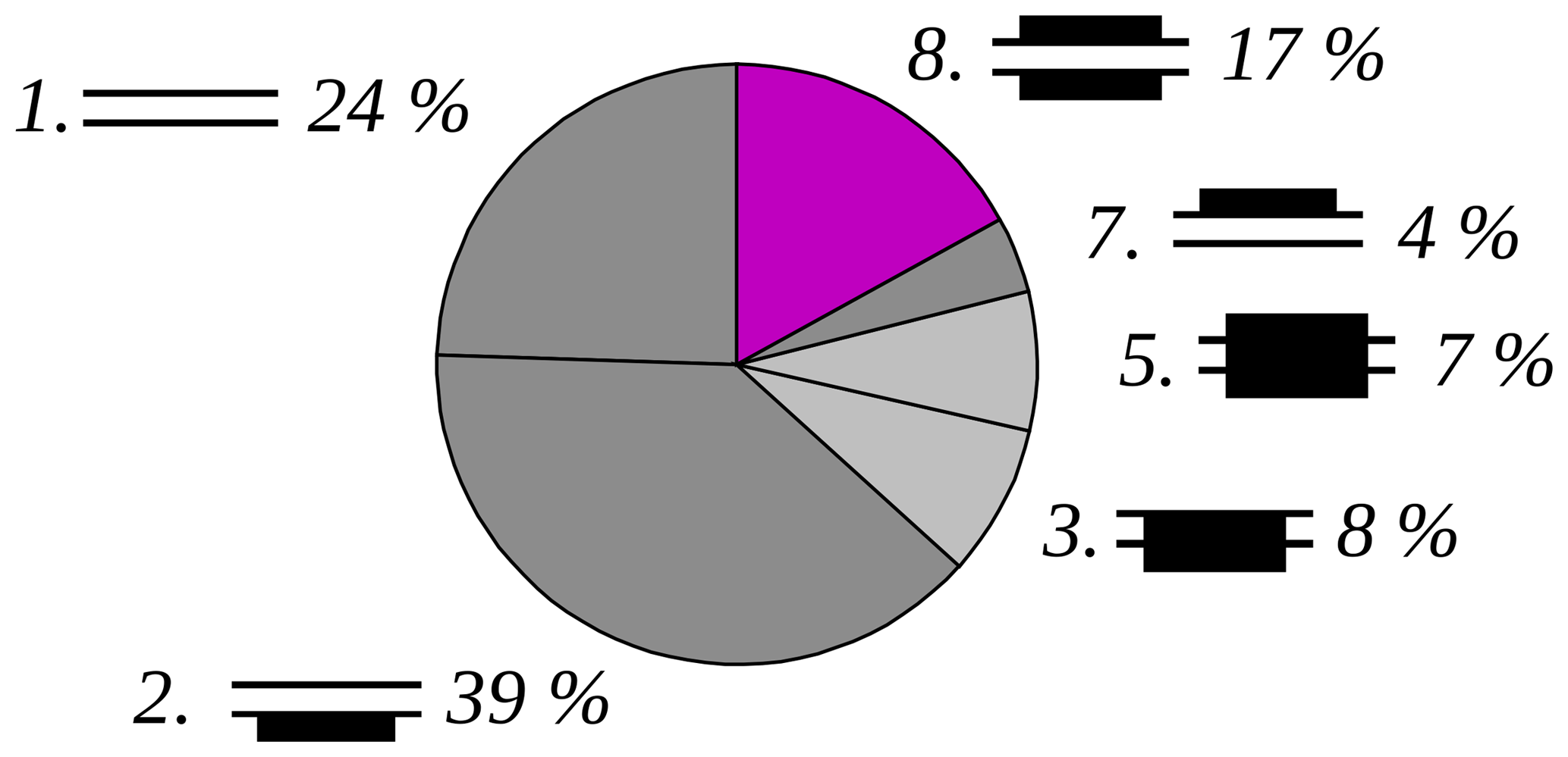
Figure 7 Non-seeding cases. Cloud categories of all non-seeding subsaturated layers. “In between” refers to the subsaturated layer. “Above” and “below” refer to the supersaturated layers above or below the subsaturated layer. A total of 100 % equals all non-seeding subsaturated layers. Non-seeding is calculated using a hexagonal plate of initial size r=400 µm. The values are rounded to zero decimal places.

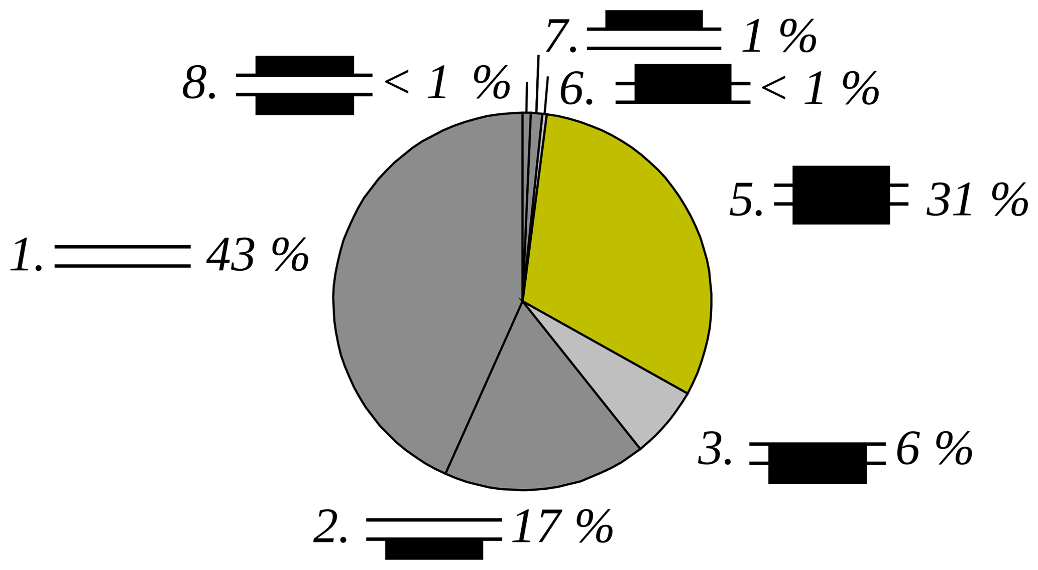
Figure 8 Seeding cases. Cloud categories of all seeding subsaturated layers. “In between” refers to the subsaturated layer. “Above” and “below” refer to the supersaturated layers above or below the subsaturated layer. A total of 100 % equals all seeding subsaturated layers. Seeding is calculated using a hexagonal plate of initial size r=400 µm. The values are rounded to zero decimal places.

In Fig. 9 the result of the cloud classification step 2 using both radiosonde profiles and radar is presented. MLCs occur in 29 % of the investigated profiles (6 % “only non-seeding”, red; +3 % “both seeding and non-seeding”, orange; and +20 % “only seeding MLC”, yellow). Single-layer clouds occur in 50 % of the investigated profiles (28 % “multilayer cloud by radiosounding, but single-layer cloud by radar”, turquoise; +22 % “single-layer clouds by radiosounding”, green). No cloud layer occurs in 22 % of the investigated profiles (12 % “multilayer cloud by radiosounding, but not cloud by radar”, light blue; +10 % “no cloud by radiosounding”, dark blue). A seasonal variation (Fig. 10) in between months in this 1-year dataset is very weak for the MLC categories (“only non-seeding multilayer clouds”, “both seeding and non-seeding multilayer clouds” and “only seeding multilayer clouds”). There is a slight increase in MLC occurrence between July and November and from February to March.

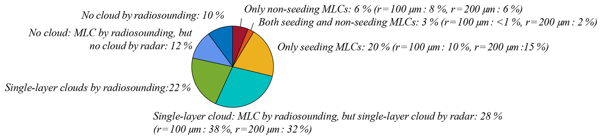
Figure 9 Cloud occurrence derived from using both radiosonde and radar for detection. For the categories the same colours as in Fig. 1 are used. A total of 100 % equals 278 days (analysed days within the 1-year dataset). Seeding and non-seeding is calculated using a hexagonal plate of initial size r=400 µm. Percentages in brackets refer to the calculations using different initial ice crystal sizes r=100 and 200 µm. The values are rounded to zero decimal places.

The impact of different ice crystal sizes used in classification step 2 is presented as numbers in brackets in Fig. 9 and as bars in Fig. 10. The main impact is that for a smaller ice crystal there are fewer “only seeding multilayer cloud” cases and more “multilayer cloud by radiosounding, but single-layer cloud by radar” cases. This is explained by the cloud category 5 (cloud above, cloud in between, cloud below) occurring frequently and sorted as MLC in the seeding cases and as single-layer cloud in the non-seeding cases. Because of this different sorting of seeding and non-seeding cases, the impact of the ice crystal size is less strong in classification step 2 compared to step 1. The impact of the different ice crystal shapes is even less, almost not visible.

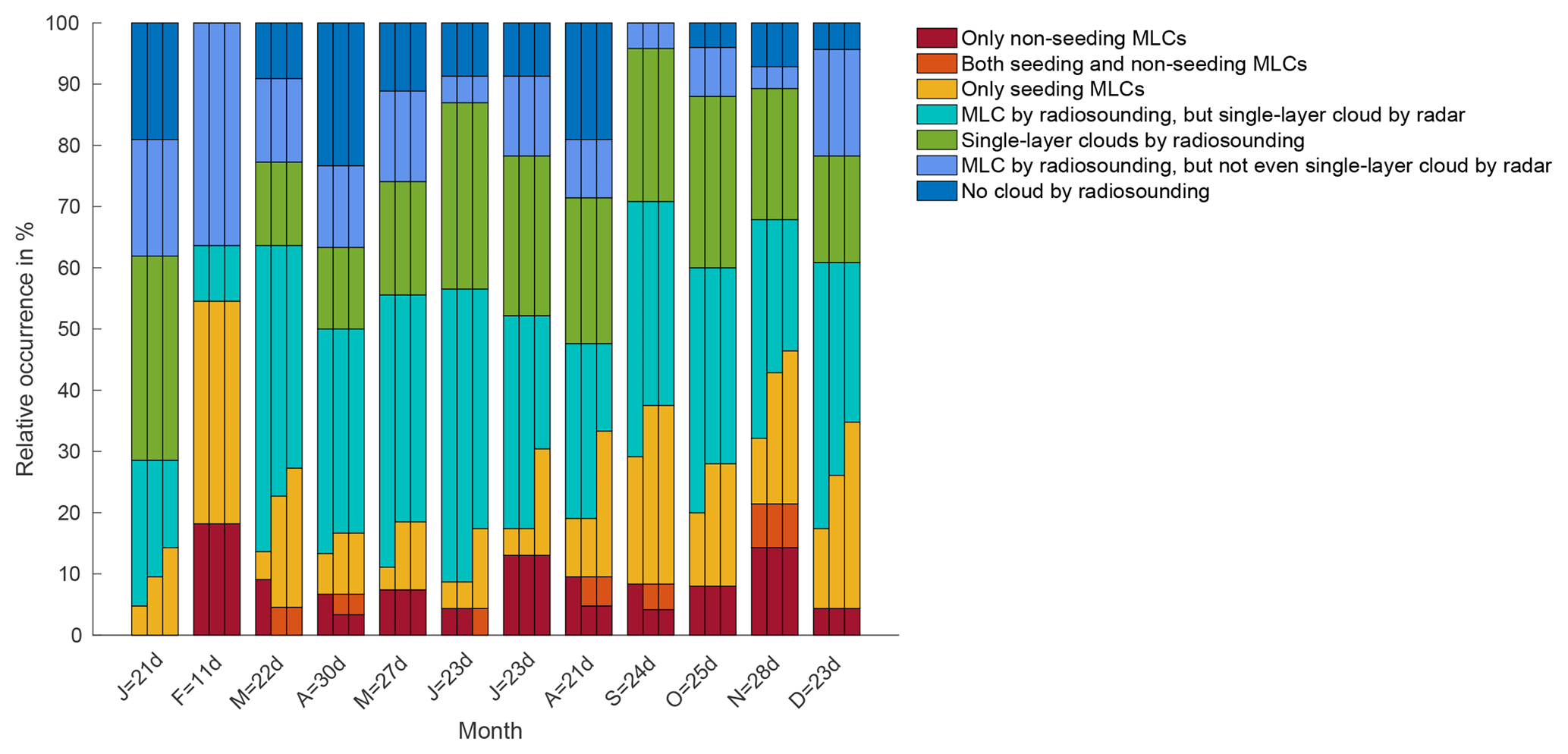
Figure 10 Temporal distribution of MLC days using classification step 2. For each month the left bar refers to the initial ice crystal size r=100 µm, the middle bar refers to the initial ice crystal size r=200 µm and the right bar refers to the initial ice crystal size r=400 µm. On the x axis the given number in the labels refers to the number of days (d) considered for the specific month.

A sensitivity study about how the results would change assuming an uncertainty of the radiosonde humidity of ±5 % is shown in Figs. A2 and A3. The measurement uncertainties lead to variations in the results of the same order of magnitude as when varying the ice crystal size. If the relative humidity is on average overestimated, the impact on the results is of smaller importance than if the relative humidity is on average underestimated. This might be explained by the minimum thickness threshold of 100 m used for identifying supersaturated and subsaturated layers, as this limits the effect of overestimating the relative humidity.

3.3 Discussion and evaluation of the results using skill scores

For evaluating the MLC occurrence derived by the classification steps 1 and 2, skill scores are used. The first classification step 1 (using only radiosonde data) is compared to classification step 2 (using both radiosonde and radar). Secondly classification step 2 is compared to a visual inspection. The visual inspection is done manually. We inspect the radar images and decide whether there is a visual MLC or no visual MLC. For the visual inspection we consider a shorter time period like that of the radiosonde ascent rather than the average over 1 h like the detection algorithm does. A longer radar signal only consisting of small strains is not counted as cloud and a longer radar signal containing some small cloud-free holes is counted as cloud.

The variables A, B, C and D needed for deriving the skill scores are given as in Table 2. Based on these variables the probability of detection (POD) is defined as

$$\begin{array}{}\text{(7)}& {\displaystyle }\mathrm{POD}={\displaystyle \frac{A}{A+C}}\end{array}$$

and shows perfect detection at POD =1 and no detection at POD =0.

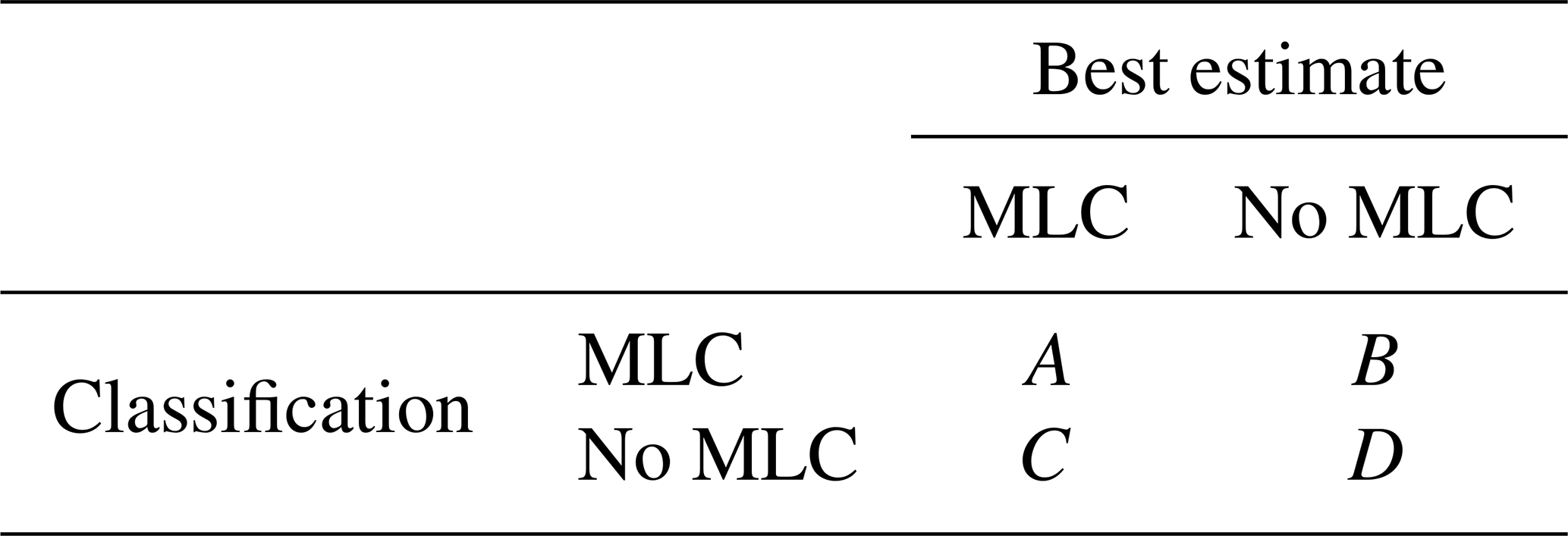
Table 2 Skill score evaluation. Definitions of the evaluation variables A, B, C and D used for the evaluation of the MLC occurrence derived by the classification steps 1 and 2 in comparison to a best estimate of MLC occurrence.

The false alarm rate FAR is defined as

$$\begin{array}{}\text{(8)}& \mathrm{FAR}={\displaystyle \frac{B}{A+B}}\end{array}$$

and gives FAR =0 for no false alarms and FAR =1 for only false alarms.

The Heidke skill score (HSS),

$$\begin{array}{}\text{(9)}& \mathrm{HSS}=\mathrm{2}{\displaystyle \frac{AD-BC}{(A+C)(C+D)+(A+B)(B+D)}},\end{array}$$

evaluates the total predictability with values reaching from HSS $=-\mathrm{\infty }$ to 1. HSS =0 means that there is no predictability.

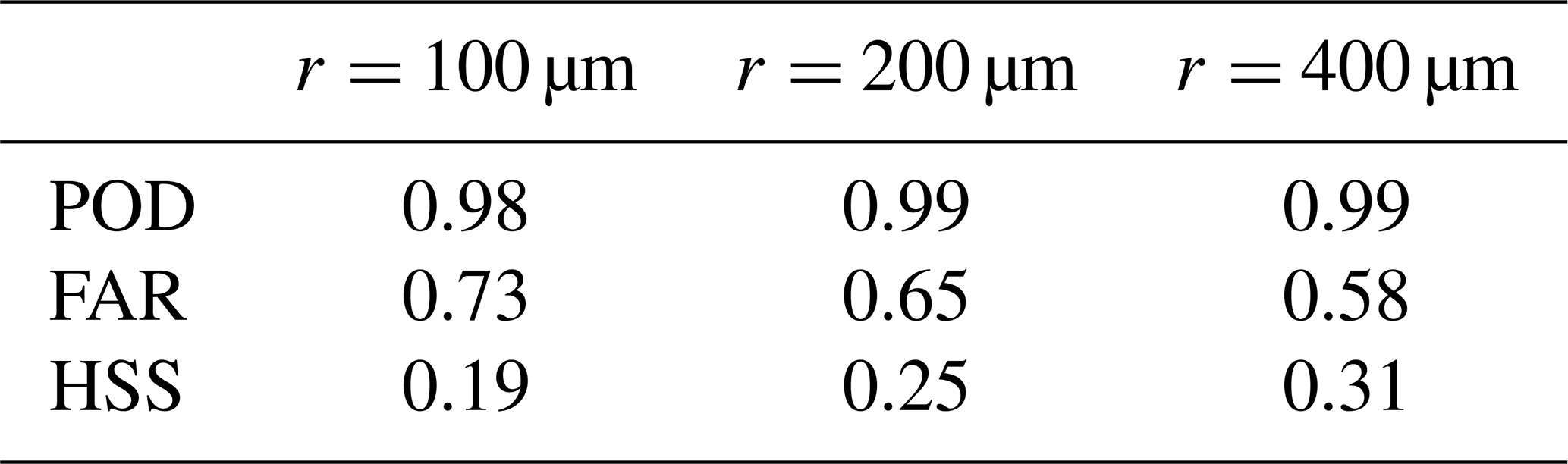
For the evaluation of classification step 1 (using only radiosonde) the variables A, B, C and D are presented in Table 3. There the results of classification step 1 are divided into MLC and no MLC. MLCs in classification step 1 are defined as one supersaturated layer above, one subsaturated layer in between and one supersaturated layer below. If a MLC is detected by classification step 1, the best estimate for evaluation is given by classification step 2 (MLC or no MLC by radar). If no MLC is detected by classification step 1, the best estimate for evaluation is done by the manual visual inspection of the radar images. The manual visual inspection is necessary owing to the non-existence of classification step 2 if there is no MLC by radiosounding. In Table 3 we see that classification step 1 represents a reliable upper limit ($\mathrm{28.8}\mathit{\%}+\mathrm{39.6}\mathit{\%}=\mathrm{68.4}\mathit{\%}$) for identifying MLC days, but the actual number might be as low as less than half (28.8 %). In Table 4 the resulting skill scores are shown. The limited predictability leads to a low Heidke skill score of HSS =0.31 for r=400 µm. The good POD of 0.99 (for r=400 µm) affirms that there is no big loss of MLC cases when applying classification step 1 (only 0.4 % for r=400 µm). FAR being 0.58 reveals that about half of the MLC estimated from radiosonde humidity measurements is “no MLC by radar”. It becomes clear that the use of the radiosonde data on their own does not reliably identify the occurrence of MLCs but can be used in combination with radar data to give information on the presence of MLCs. Reducing the initial ice crystal size to r=100 or r=200 µm shows a reduced Heidke skill score. This indicates that the chosen initial ice crystal size impacts the predictability.

Table 3 Evaluation of the MLC results of radiosonde detection (classification step 1) in comparison to radar detection (classification step 2). “MLC by radar” is given by cloud category 8 for the non-seeding cases and by cloud category 5 for the seeding cases. The evaluation is done for the ice crystal sizes r=100, 200 and 400 µm. The values are rounded to one decimal place.

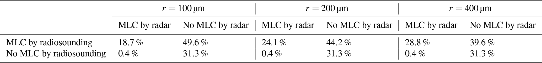
Table 4 Skill scores for comparison of MLC results of radiosounding and radar. The skill scores are calculated for the ice crystal sizes r=100, 200 and 400 µm. The values are rounded to two decimal places.

Next we evaluate classification step 2 and the results are presented in Tables 5 and 6. Due to the missing possibility to distinguish falling ice crystals from cloud particles in the radar image, including seeding in our classification leads to high uncertainties. Therefore for evaluating classification step 2, we only consider the non-seeding MLCs (cloud category 8). This is a similar approach to that by Intrieri et al. (2002), who defined MLCs as two separate clouds with a clear visible interstice in between. For the evaluation of classification step 2 we use the manual visual inspection as a best estimate. Also for the manual visual inspection we do not account for the possibility of seeding, meaning that we count a connected radar signal in the vertical as single-layer cloud.

Table 5 Evaluation of the MLC results including only the non-seeding MLC of the classification step 2 in comparison to manual visual detection. “Non-seeding MLC” includes “only non-seeding” and “both seeding and non-seeding” MLC. “Seeding MLC and no MLC” includes seeding MLCs, single-layer clouds and no cloud layers. The evaluation is done for the ice crystal sizes r=100, 200 and 400 µm. The values are rounded to one decimal place.

Classification step 2 classifies 7.9 % of MLCs (r=400 µm in Table 5). This represents a lower limit for identifying MLC days, since classification step 2 is not able to classify 10.4 % (4.0 % is classified as seeding MLC and 6.1 % as no MLC). The actual number of MLCs might therefore be twice as high ($\mathrm{7.9}\mathit{\%}+\mathrm{10.4}\mathit{\%}=\mathrm{18.3}\mathit{\%}$ for r=400 µm). This limited probability is underlined by POD being 0.43 (Table 6). Problems of the classification are given by the inexact accordance between the radiosonde profile and radar. While the radiosonde ascends, it is horizontally drifted away from the radar by wind. Additionally the radar measurements have to be averaged over time and this is not done by the visual inspection. An existing cloud, which is too weak or too short lasting in the radar image, can therefore lead to discrepancies between the classification and the visual detection. A too-high cloud top or base compared to the relative humidity threshold, a missing relative humidity layer or too many relative humidity layers in an unchanging radar image do also cause erroneous classification.

Table 6 Skill scores for comparison of MLC results of the non-seeding cases of the classification step 2 and the visual detection. The skill scores are calculated for the ice crystal sizes r=100, 200 and 400 µm. The values are rounded to two decimal places.

However, few false alarms (0.7 % for r=400 µm) cause a low FAR of 0.08. This reveals predictability by a Heidke skill score of 0.53. Using the smaller radius of r=200 µm does not change the results. Even if there is less seeding, these cases belong to the category “both seeding and non-seeding” and therefore do not change the results. Using the even smaller radius of r=100 µm does impact the results. In classification step 1 the larger radii r=200 and r=400 µm lead to the best Heidke skill score (HSS =0.25 and 0.31) in comparison to the small radius. However, in classification step 2 the smaller radius r=100 µm leads to the best Heidke skill score (HSS =0.55). Even if the large radius of r=400 µm is likely in mixed-phase MLCs (Mioche et al., 2017), it is possible that it does not occur as often as a radius of r=100 µm.

4 Conclusions

In this work we use in situ profiling by radiosondes and ground-based remote sensing by vertically pointing cloud Doppler radar to identify Arctic MLCs between 0 and 10 km height. We evaluate relative humidity profiles regarding an ice-subsaturated layer in between two ice-supersaturated layers. This combination occurs on 68.4 % of the 278 analysed days (only 1 h each day is analysed) using the minimum considered thickness for the supersaturated and subsaturated layers of 100 m. A high amount of supersaturated layers found in the radiosonde profiles does not coincide with observed cloud occurrence. This is probably due to lack of CCN and INPs and thereby missing cloud formation. Only using radiosonde profiles is not sufficient for the detection of clouds. Therefore the classification is extended by using radar data for excluding non relevant cases. The extended classification leads to 29 % MLCs with a very weak seasonal cycle. We investigate these MLC further regarding the possibility of seeding, which means if an ice crystal of the size r=400 µm does not fully sublimate (survive) in the subsaturated layer when falling through this layer. We find that seeding can potentially occur on 23 % of the 278 investigated days. In these cases there is a radar signal in the subsaturated layer in between the two cloud layers. Here it remains as an unsolved question of whether this is actually due to seeding (falling ice crystals in between the two cloud layers) or due to one continuous cloud layer. Since the percentage for potential seeding is as high as 23 %, the importance of seeding for the lower cloud is not negligible. The effects of the seeding on the lower cloud could be an increase in cloud ice and thereby precipitation formation and cloud dissipation. In order to gain more information about the existence of these seeding ice crystals, further measurements of for example lidar would be needed but were not available during the observation time period.

Non-seeding means that the subsaturated layer is too thick or too dry for the ice crystal to survive the sublimation. Non-seeding MLCs are visible in the radar as two separated cloud layers. This occurs in 9 % of the analysed days. Following from our sublimation calculation we find that MLCs visibly separated in the radar are unable to interact through seeding. However, we have to keep uncertainties like the radar detection limit in mind. In the case of non-seeding MLCs, radiative interactions, like a weakening of the lower cloud in the existence of a higher cloud, can occur. These interactions are most likely not captured correctly by weather models. However, the 9 % occurrence implies that clearly separated MLCs should probably not be neglected in weather models.

Cloud detection by satellites is challenging in the Arctic, but Liu et al. (2012) found that Arctic MLCs occur between 17 % and 25 % of the investigated time. However, since the minimum considered cloud thickness was as big as 960 m, they assumed their MLC amount most likely to be underestimated. In order to evaluate our classification we compare our results to a manual visual inspection of the radar observations. Since the seeding cases can not be separated from single-layer cloud cases and therefore cause uncertainties, the seeding cases are excluded in the evaluation. The evaluation results in a non-seeding MLC occurrence of 9 % being a reliable lower limit. However, the Heidke skill score HSS for prediction is only 0.53. Changing the ice crystal size has various impacts. For smaller ice crystal sizes the impact on the results is larger. However, the skill score analysis showed no clear answer about the best choice of ice crystal size. Erroneous detection is often caused by super- and subsaturated layers identified in the radiosonde data not overlapping with the radar cloud top and base. Also non-relevant, often thin super- and subsaturated layers cause problems. Here the uncertainties in the relative humidity measurements and the chosen minimum height limits have to be kept in mind when examining these disagreements. The manual visual inspection results in an 18.4 % non-seeding MLC occurrence.

Using our ground-based classification leads to a MLC occurrence between 8 % and 29 % for Ny-Ålesund. If and how much this number will differ at a more typical high-Arctic location, with less cyclonic and orographic influence but rather stable conditions caused by sea ice, remains an unsolved question. We show that seeding is more frequently possible than non-seeding and always causes a signal in the radar. Therefore uncertainties remain when distinguishing MLC from single-layer clouds in radar images. While extensive modelling studies (e.g. Klein et al., 2009 and Ovchinnikov et al., 2014) have dealt with single-layer Arctic clouds, we suggest that the more complex microphysics and radiative properties of MLCs and their changes due to aerosol and climate perturbations should be a focus of future research.

Appendix A

Table A1 Calculation of capacitance based on Westbrook et al. (2008). The listed ice crystal shapes correspond to the selected particles' hexagonal plates, rimed long columns, crystal with sector-like branches and assemblages of planar polycrystals respectively (Mitchell, 1996). 2a refers to the maximum span across the basal/hexagonal face (Westbrook et al., 2008). In the case of the hexagonal plate and the star crystal this is a=r. In the case of a hexagonal column it is $a=\mathrm{2}r/A$, with 2r being the maximum dimension. The fall speed is calculated using r=400 µm, T=253.15 K and p=1013.15 hPa.

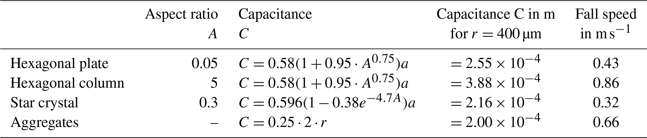
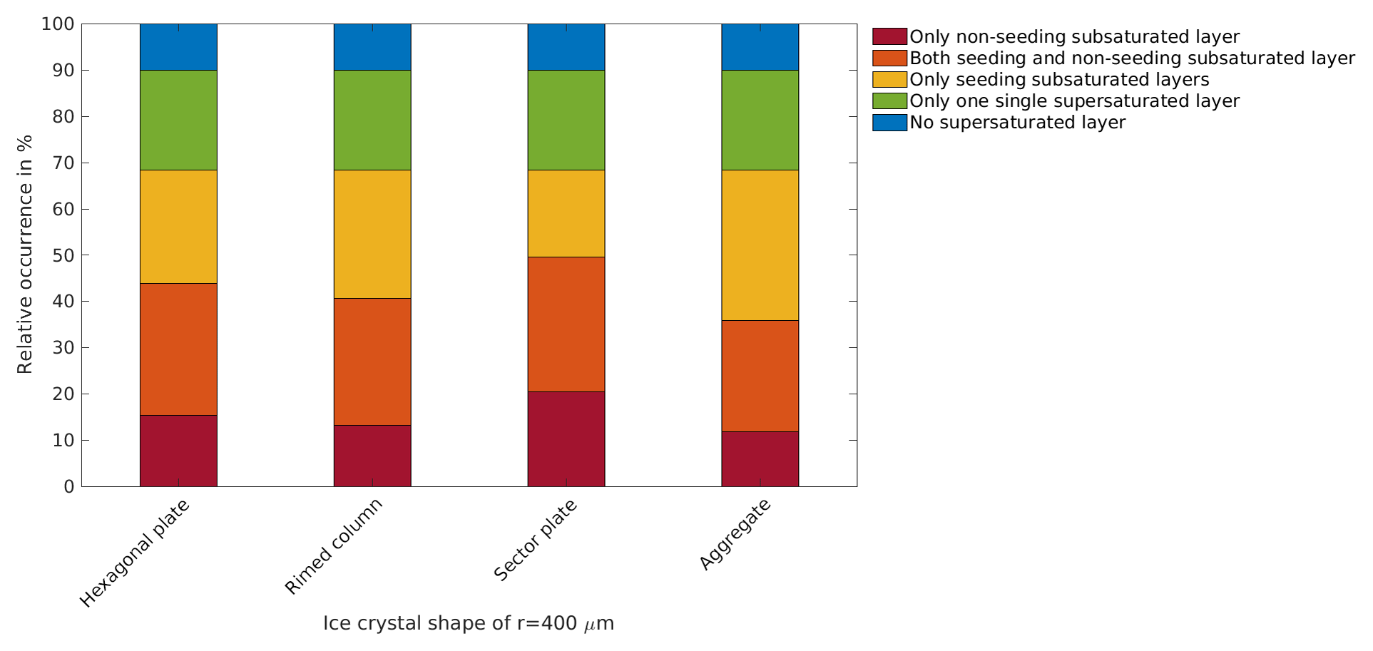
Figure A1 Cloud occurrence derived by using classification step 2 using the four different ice crystal shapes: hexagonal plate, rimed column, sector plate and aggregate. The initial ice crystal size is r=400 µm.

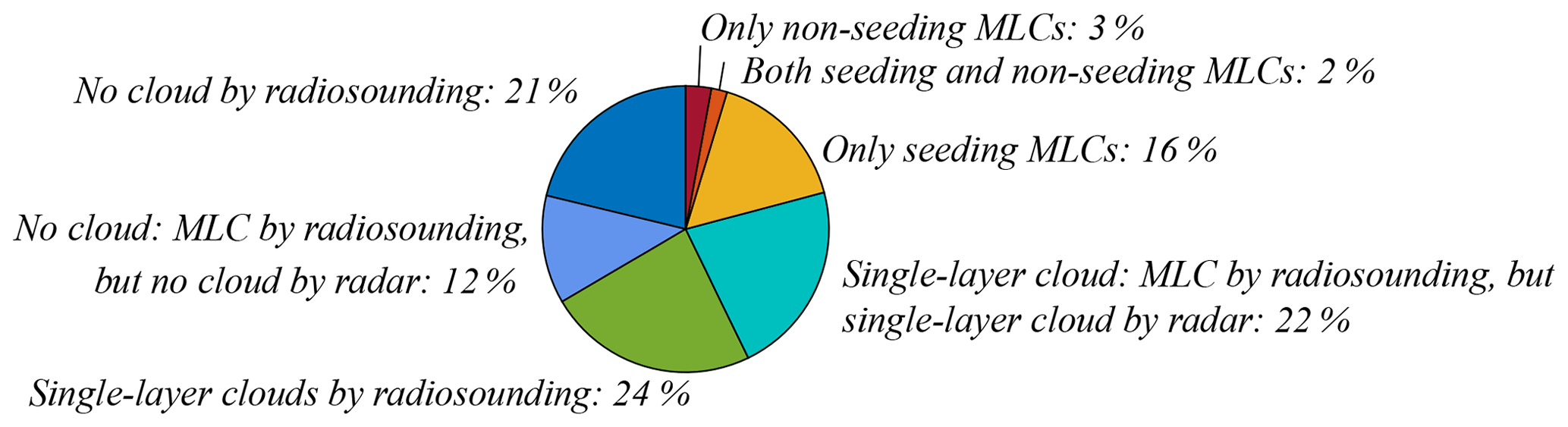
Figure A2 Cloud occurrence derived from using both radiosonde and radar for detection. For the radiosonde data the measurement uncertainty is considered to be −5 % relative humidity over the whole radiosonde profile. Seeding and non-seeding is calculated using an ice crystal of the size r=400 µm. The values are rounded to zero decimal places.

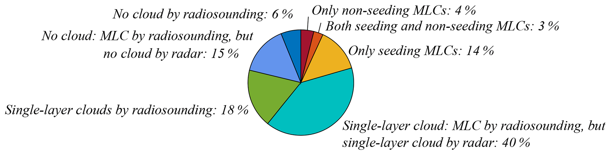
Figure A3 Cloud occurrence derived from using both radiosonde and radar for detection. For the radiosonde data the measurement uncertainty is considered to be +5 % relative humidity over the whole radiosonde profile. Seeding and non-seeding is calculated using an ice crystal of the size r=400 µm. The values are rounded to zero decimal places.