Exploring accumulation-mode H₂SO₄ versus SO₂ stratospheric sulfate geoengineering in a sectional aerosol–chemistry–climate model

Stratospheric sulfate geoengineering (SSG) could contribute to avoiding some of the adverse impacts of climate change. We used the SOCOL-AER global aerosol–chemistry–climate model to investigate 21 different SSG scenarios, each with 1.83 Mt S yr⁻¹ injected either in the form of accumulation-mode H₂SO₄ droplets (AM H₂SO₄), gas-phase SO₂ or as combinations of both. For most scenarios, the sulfur was continuously emitted at an altitude of 50 hPa (≈20 km) in the tropics and subtropics. We assumed emissions to be zonally and latitudinally symmetric around the Equator. The spread of emissions ranged from 3.75^∘ S–3.75^∘ N to 30^∘ S–30^∘ N. In the SO₂ emission scenarios, continuous production of tiny nucleation-mode particles results in increased coagulation, which together with gaseous H₂SO₄ condensation, produces coarse-mode particles. These large particles are less effective for backscattering solar radiation and have a shorter stratospheric residence time than AM H₂SO₄ particles. On average, the stratospheric aerosol burden and corresponding all-sky shortwave radiative forcing for the AM H₂SO₄ scenarios are about 37 % larger than for the SO₂ scenarios. The simulated stratospheric aerosol burdens show a weak dependence on the latitudinal spread of emissions. Emitting at 30^∘ N–30^∘ S instead of 10^∘ N–10^∘ S only decreases stratospheric burdens by about 10 %. This is because a decrease in coagulation and the resulting smaller particle size is roughly balanced by faster removal through stratosphere-to-troposphere transport via tropopause folds. Increasing the injection altitude is also ineffective, although it generates a larger stratospheric burden, because enhanced condensation and/or coagulation leads to larger particles, which are less effective scatterers. In the case of gaseous SO₂ emissions, limiting the sulfur injections spatially and temporally in the form of point and pulsed emissions reduces the total global annual nucleation, leading to less coagulation and thus smaller particles with increased stratospheric residence times. Pulse or point emissions of AM H₂SO₄ have the opposite effect: they decrease the stratospheric aerosol burden by increasing coagulation and only slightly decrease clear-sky radiative forcing. This study shows that direct emission of AM H₂SO₄ results in higher radiative forcing for the same sulfur equivalent mass injection strength than SO₂ emissions, and that the sensitivity to different injection strategies varies for different forms of injected sulfur.

1 Introduction

Driven by human emissions, long-lived atmospheric greenhouse gas (GHG) concentrations now exceed levels ever experienced by Homo sapiens. The effects of these GHGs – as written by the Intergovernmental Panel on Climate Change in 2014 – “have been detected throughout the climate system and are extremely likely to have been the dominant cause of the observed warming since the mid-20th century” (IPCC, 2014). Emissions of CO₂ and other GHGs must be curbed to reduce the impacts of climate change. Yet, the long lifetime of CO₂ and some other GHGs suggest that even if emissions were eliminated today, climate change and resulting human and environmental risks would persist for centuries.

We might bring global warming to a halt or reduce its rate of growth by combining emission cuts with other interventions, such as a deliberate increase in the Earth's stratospheric aerosol burden, which would enhance the albedo of the stratospheric aerosol layer and reduce solar climate forcing. This idea, now often called “solar geoengineering”, “solar climate engineering” or “solar radiation management”, was first proposed by Budyko (1977), who suggested injecting sulfate aerosols into the stratosphere to increase Earth's albedo. Research on this topic became tabooed because of the risks entailed. However, efforts were renewed after Crutzen (2006) suggested that solar radiation management might be explored as a useful climate change mitigation tool, as adequate emission reductions were becoming increasingly unlikely.

Most research on solar geoengineering has focused on stratospheric sulfate geoengineering (SSG) via SO₂ injection, in part due to its volcanic analogues such as the 1991 eruption of Mt. Pinatubo. However, studies of SSG have found limitations regarding SO₂ injection as a method of producing a radiative forcing (RF) perturbation. These limitations include the following: (1) reduced efficacy at higher loading, limiting the achievable shortwave (SW) radiative forcing (Heckendorn et al., 2009; Niemeier et al., 2011; English et al., 2012; Niemeier and Timmreck, 2015; Kleinschmitt et al., 2018); (2) increased lifetimes of methane and other GHGs (Visioni et al., 2017; Tilmes et al., 2018); (3) impacts on upper tropospheric ice clouds (Kuebbeler et al., 2012; Visioni et al., 2018b); and (4) stratospheric heating (Heckendorn et al., 2009; Ferraro et al., 2011), especially in the tropical lower stratosphere, which would modify the Brewer–Dobson circulation (Brewer, 1949; Dobson, 1956) and increase stratospheric water vapor. Limitation (1) is primarily a function of the sulfate particle size distribution, determining their gravitational removal, whereas (2) to (4) are primarily dependent on chemical and radiative particle properties.

The size distribution problem regarding SO₂ injection arises after oxidation of SO₂ to H₂SO₄ when aerosol particles are formed through nucleation and condensation. Condensation onto existing particles increases their average size. In addition, the continuous flow of freshly nucleated particles leads to coagulation, both via the self-coagulation of the many small new particles and – more importantly – coagulation with preexisting bigger particles from the background aerosol layer. These particles then grow further via coagulation and condensation, which increases the average sedimentation velocity of the aerosol population (Heckendorn et al., 2009). Mean particle sizes tend to increase with the SO₂ injection rate, reducing the stratospheric aerosol residence time and, hence, their radiative forcing efficacy (e.g., W m⁻² (Mt S yr${}^{-\mathrm{1}}{)}^{-\mathrm{1}})$. This problem could be reduced – and the radiative efficacy increased – if there was a way to produce additional accumulation-mode (0.1–1.0 µm radius) sulfate particles (AM H₂SO₄). Such particles are large enough to decrease their mobility and, in turn, their coagulation. Furthermore, such particles are close to the radius of maximum mass specific up-scattering of solar radiation on sulfate particles, which is ∼0.3 µm (Dykema et al., 2016). One proposed method of doing this is to directly inject H₂SO₄ vapor into a rapidly expanding aircraft plume during stratospheric flight, which would be expected to lead to the formation of accumulation-mode particles with a size distribution that depends on the injection rate and the expansion characteristics of the plume (Pierce et al., 2010). Two theoretical studies, Pierce et al. (2010) and Benduhn et al. (2016), suggest that appropriate size distributions could be produced in aircraft plumes using this method.

To evaluate a geoengineering approach with AM H₂SO₄ one needs to study the evolution of aerosol particles after the injection of H₂SO₄ vapor into an aircraft wake and the subsequent transport and evolution of the aerosol plume around the globe. This is a problem with temporal scales ranging from milliseconds to years and spatial scales from millimeters to thousands of kilometers. At present there is no model that could seamlessly handle the entire range. However, the problem can be divided into two separate domains: (a) from injection to plume dispersal and (b) from plume dispersal to global-scale distribution. Each domain has associated uncertainties, but these can be studied separately with different modeling tools: plume dispersion models for (a) and general circulation models (GCMs) or chemistry–climate models (CCMs) for (b).

• (a)

  Plume modeling. The integration of the plume model starts with the production of small particles in a plume from the exit point of the injection nozzle, and ends when the plume has expanded sufficiently so that the loss of particles by coagulation with ambient particles dominates the self-coagulation, whereupon the GCM or CCM becomes the appropriate tool (Pierce et al., 2010). The plume model needs to account for the initial formation of nucleation-mode particles below a radius of 0.01 µm by homogeneous nucleation of H₂SO₄ and H₂O vapor and the subsequent evolution of the particle size distribution by coagulation of the nucleation mode, as well as by condensation of H₂SO₄ vapor on existing particles. In an expanding aircraft plume, these processes occur on timescales from milliseconds to hours and length scales from millimeters to kilometers. This was addressed by Pierce et al. (2010) and then by Benduhn et al. (2016). There is rough agreement that particles between a radius of 0.095 and 0.15 µm could be produced after the initial plume processing, but these results are subject to uncertainties and need further investigation.

• (b)

  General circulation modeling. The second part of the problem can be analyzed using a GCM or a CCM, starting from the release of sulfate particles of the size distribution calculated by the plume model into the grid of the GCM, all the way to implications on aerosol burden, radiative forcing, ozone, stratospheric temperature and circulation. To this end, the GCM must be coupled to chemistry and aerosol modules. The GCM then provides solutions on how the new accumulation-mode particles change the large-scale size distribution, and thus the overall radiative and dynamical response to sulfate aerosol injection. Missing in this methodology are processes smaller than the grid size of the GCM, which may involve filaments of injected material being transported in thin layers. Consideration of these sub-grid-scale processes remains an uncertainty in our study, but might be handled by a Lagrangian transport model in a future study.

A sectional (or size-bin resolved) aerosol module is important for a mechanistic understanding of the factors that determine the size distributions of the aerosols. Sectional aerosol models handle the aerosols in different size bins (40 in SOCOL-AER), whereas modal models usually only apply three modes (e.g., Niemeier et al., 2011; Tilmes et al., 2017), each with different mode radius (r_m) and fixed distribution widths (σ), to describe the aerosol distribution. Therefore, the degrees of freedom among modal models usually is 3, whereas there are 40 for a sectional model such as SOCOL-AER. Thus, sectional aerosol models represent aerosol distributions with better accuracy, although numerical diffusion does result from the discretization in size space. Two earlier studies of SSG modeling, Heckendorn et al. (2009) and Pierce et al. (2010), used the AER-2D chemistry–transport–aerosol model with sectional microphysics (Weisenstein et al., 1997, 2007). Although the sectional aerosol module within has high size resolution, this 2-D model only has a limited spatial resolution with simplified dynamical processes. So far, various studies have used four different GCM models to investigate SSG with sectional aerosol modules, namely English et al. (2012), Laakso et al. (2016, 2017), Visioni et al. (2017, 2018a, b) and Kleinschmitt et al. (2018). English et al. (2012) used the WACCM GCM (Garcia et al., 2007) coupled to the sectional aerosol module CARMA (Toon et al., 1988) to simulate various SSG scenarios with sulfur emissions in the form of SO₂ gas, H₂SO₄ gas and AM H₂SO₄, but without treatment of the quasi-biennial oscillation (QBO) and without online interaction between aerosols, chemistry and radiation. The three other studies (Laakso et al., 2016, 2017; Visioni et al., 2017, 2018a, b; Kleinschmitt et al., 2018) only performed SO₂ emission scenarios, but no AM H₂SO₄ emission scenarios. Laakso et al. (2016, 2017) used the MA-ECHAM5 GCM interactively coupled to the sectional aerosol module HAM-SALSA (Kokkola et al., 2008; Bergman et al., 2012); however, in both studies stratospheric chemistry was simplified using prescribed monthly mean OH and ozone concentrations. The ULAQ-CCM, which was used in Visioni et al. (2017, 2018a, b), includes an interactive sectional aerosol module and additionally treats detailed stratospheric chemistry. Kleinschmitt et al. (2018) used the LMDZ GCM (Hourdin et al., 2006, 2013) which was coupled to the S3A sectional aerosol module (Kleinschmitt et al., 2017). In their model setup, the aerosols were fully interactive with the radiative scheme, but the model included only simplified chemistry and a prescribed SO₂-to-H₂SO₄ conversion rate.

There have been prior studies with other advanced interactive GCMs, but using modal aerosol schemes. Niemeier et al. (2011) looked at SO₂ and H₂SO₄ gas injection by using the MA-ECHAM GCM interactively coupled to the HAM modal aerosol module (Stier et al., 2005). Chemistry was simplified in a similar fashion to Laakso et al. (2016, 2017) using prescribed OH and ozone concentrations. Kravitz et al. (2017), MacMartin et al. (2017), Richter et al. (2017) and Tilmes et al. (2017) used the CESM1 fully coupled global chemistry–climate model (Hurrell et al., 2013; Mills et al., 2017) to simulate SO₂ emission scenarios. In their model setup, they applied higher horizontal and vertical resolutions compared with SOCOL-AER as well as a fully coupled ocean module and more complex chemistry. However, they also relied on a modal aerosol module, which in turn was coupled to cloud microphysics.

In this study we investigate different SO₂ and AM H₂SO₄ emission scenarios using the SOCOL-AER sectional global 3-D aerosol–chemistry–climate model (Sheng et al., 2015), which treats prognostic transport as well as radiative and chemical feedbacks of the aerosols online in one model. As described above, GCMs are not yet able to interactively couple plume dispersion models. Hence, we follow Pierce et al. (2010) and use a log-normal distribution for the injected aerosols in the AM H₂SO₄ emission scenarios, assuming that a certain size distribution can be created in an emission plume (Pierce et al., 2010; Benduhn et al., 2016). SO₂ emission scenarios are performed as a reference, and to gain insight into aerosol formation processes on a global scale. We perform a number of sensitivity studies with both SO₂ and AM H₂SO₄ emissions that highlight differences between the two injection strategies and indicate future research needs.

2 Model description

We use the SOCOL-AER global 3-D aerosol–chemistry–climate model (Sheng et al., 2015) in this study. Earlier geoengineering research by Heckendorn et al. (2009) used SOCOLv2 (Egorova et al., 2005; Schraner et al., 2008) to study the stratospheric response to SO₂ injections. In that case, the AER-2D model (Weisenstein et al., 1997, 2007) was used to calculate global aerosol properties, which were prescribed in the SOCOLv2 3-D chemistry–climate model. The SOCOL-AER (Sheng et al., 2015; Sukhodolov et al., 2018) model is based on SOCOLv3 (Stenke et al., 2013) and improves on the earlier versions of SOCOL by incorporating a sectional aerosol module based on the AER-2D model. In a recent study SOCOL-AER was successfully applied to simulate the magnitude and the decline of the resulting aerosol plume after the 1991 Mt. Pinatubo eruption (Sukhodolov et al., 2018).

SOCOL-AER includes the chemistry of the sulfate precursors H₂S, CS₂, dimethyl sulfide (C₂H₆S, DMS), OCS, methanesulfonic acid (CH₄O₃S, MSA), SO₂, SO₃ and H₂SO₄, as well as the formation and evolution of particulates via particle size resolving microphysical processes such as homogeneous bimolecular nucleation of H₂SO₄ and H₂O, condensation and evaporation of H₂SO₄ and H₂O, coagulation, and sedimentation. As opposed to an earlier version of SOCOL-AER that used a wet radius binning scheme (Sheng et al., 2015), this model version separates the aerosol according to H₂SO₄ mass into 40 bins, with H₂SO₄ mass doubling between neighboring bins. The new binning approach allows for more accurate consideration of size distribution changes caused by evaporation and condensation of H₂O on the sulfate aerosols. Depending on the grid-box temperature and relative humidity, wet aerosol radii in the new scheme can range from 0.4 nm to 7 µm. Nevertheless, to simplify post-processing of results the sulfate aerosols are rebinned into the original wet size bins of Sheng et al. (2015). SOCOL-AER interactively couples the AER aerosol module with the MEZON chemistry module (Rozanov et al., 1999, 2001; Egorova et al., 2001, 2003) via photochemistry of the sulfate precursor gases as well as heterogeneous chemistry on the particle surfaces. In SOCOL-AER, MEZON treats 56 chemical species of oxygen, nitrogen, hydrogen, carbon, chlorine, bromine and sulfur families with 160 gas-phase reactions, 58 photolysis reactions, and 16 heterogeneous reactions, representing the most relevant aspects of stratospheric chemistry. SOCOL-AER also treats tropospheric chemistry, although with a reduced set of organic chemistry (isoprene as most complex organic species), and prescribed aerosols (other than sulfate aerosols, which are fully coupled). SOCOL-AER also interactively couples AER with the ECHAM5.4 GCM (Manzini et al., 1997; Roeckner et al., 2003, 2006) of SOCOLv3 via the radiation scheme. SOCOL-AER treats 6 SW radiation bands between 185 nm and 4 µm as well as 16 longwave radiation bands in the spectral range from 10 to 3000 cm⁻¹. The extinction coefficients, which are required for each of the 22 wavelengths, as well as the single scattering albedo and the asymmetry factors, which are only taken into account for the six SW bands, are calculated from the particle size distribution of the 40 size bins according to Mie scattering theory (Biermann et al., 2000), with radiative indexes from Yue et al. (1994). The transport of the sulfur gas species and the aerosol bins is integrated into the ECHAM5 advection scheme (Lin and Rood, 1996). MEZON is interactively coupled to ECHAM5 using the 3-D fields of temperature, wind and radiative forcing of water vapor, methane, ozone, nitrous oxide and chlorofluorocarbons.

Operator splitting is used, whereupon transport is calculated every 15 min, and chemistry, microphysics and radiation are calculated every 2 h, with 3 min sub-time-steps for microphysical processes. We used T31 horizontal truncation (i.e., 3.75^∘ resolution in longitude and latitude) with a vertical resolution of 39 hybrid sigma-p levels from the surface up to 0.01 hPa (i.e., an altitude of about 80 km). This results in a vertical resolution of about 1.5 km in the lower stratosphere.

This study is among the first modeling studies on SSG which couple a size-resolved sectional aerosol module interactively to well-described stratospheric chemistry and radiation schemes in a global 3-D chemistry–climate model. Furthermore, this study explores the injection of AM H₂SO₄ in detail and contrasts the resulting atmospheric effects and sensitivities with those of gaseous SO₂ injections.

3 Experimental setup

In this study, 21 different injection scenarios with annual emissions of 1.83 Mt of sulfur per year (Mt S yr⁻¹) in the form of AM H₂SO₄ (sulfate aerosols) or gaseous SO₂ were performed, as well as runs with mixtures of both species. Per year, this corresponds to about 8 %–20 % of the sulfur emitted by the 1991 Mt. Pinatubo eruption, depending on the model under consideration and the applied boundary conditions (Mills et al., 2016; Pitari et al., 2016; Sukhodolov et al., 2018; Timmreck et al., 2018). See Table 1 for a complete list of scenarios. Additionally, a reference run (termed “BACKGROUND”) without artificial sulfur emissions was conducted to enable comparison with background conditions. Natural and anthropogenic emissions of chemical species were treated as described by Sheng et al. (2015). Each simulation was performed for 20 years representing atmospheric conditions of the years 2030–2049 for ozone depleting substances (2.3 ppb Cl_Y and 18 ppt Br_Y above an altitude of 50 km; WMO, 2008) and GHG concentrations following the Representative Concentration Pathway 6.0 scenario (RCP6.0), with the first 10 years used as spin-up and the last 10 years used for analysis. Sea surface temperatures (SSTs) and sea ice coverage (SIC) were prescribed as a repetition of monthly means of the year 2001 from the Hadley Centre Sea Ice and Sea Surface Temperature 1 data set (hadISST1) by the UK Met Office Hadley Centre (Rayner et al., 2003). The QBO was taken into account by a linear relaxation of the simulated zonal winds in the equatorial stratosphere to observed wind profiles over Singapore perpetually repeating the years 1999 and 2000. The geoengineering emissions were injected at an altitude of 50 hPa (≈20 km) except for runs number 19 (termed “GEO_AERO_25km_15”) and 20 (termed “GEO_SO2_25km_15”) which emitted AM H₂SO₄ and SO₂, respectively, at about an altitude of 24 hPa (≈25 km) to investigate the sensitivity to the emission altitude.

Table 1 Overview of all simulations performed in this study. Each GEO scenario (1–12) assumes a zonally symmetric and continuous injection of 1.83 Mt S yr⁻¹ as SO₂ and/or accumulation-mode particles (AM H₂SO₄) with log-normal size distribution (dry mode radius, r_m=0.095 µm and distribution width σ=1.5). Longitudinal and latitudinal distributions as well as emission ratios of liquid to gas (in sulfur mass) are shown in columns 3–6. GEO scenarios (13–20) deviate from these standard conditions as indicated under remarks.

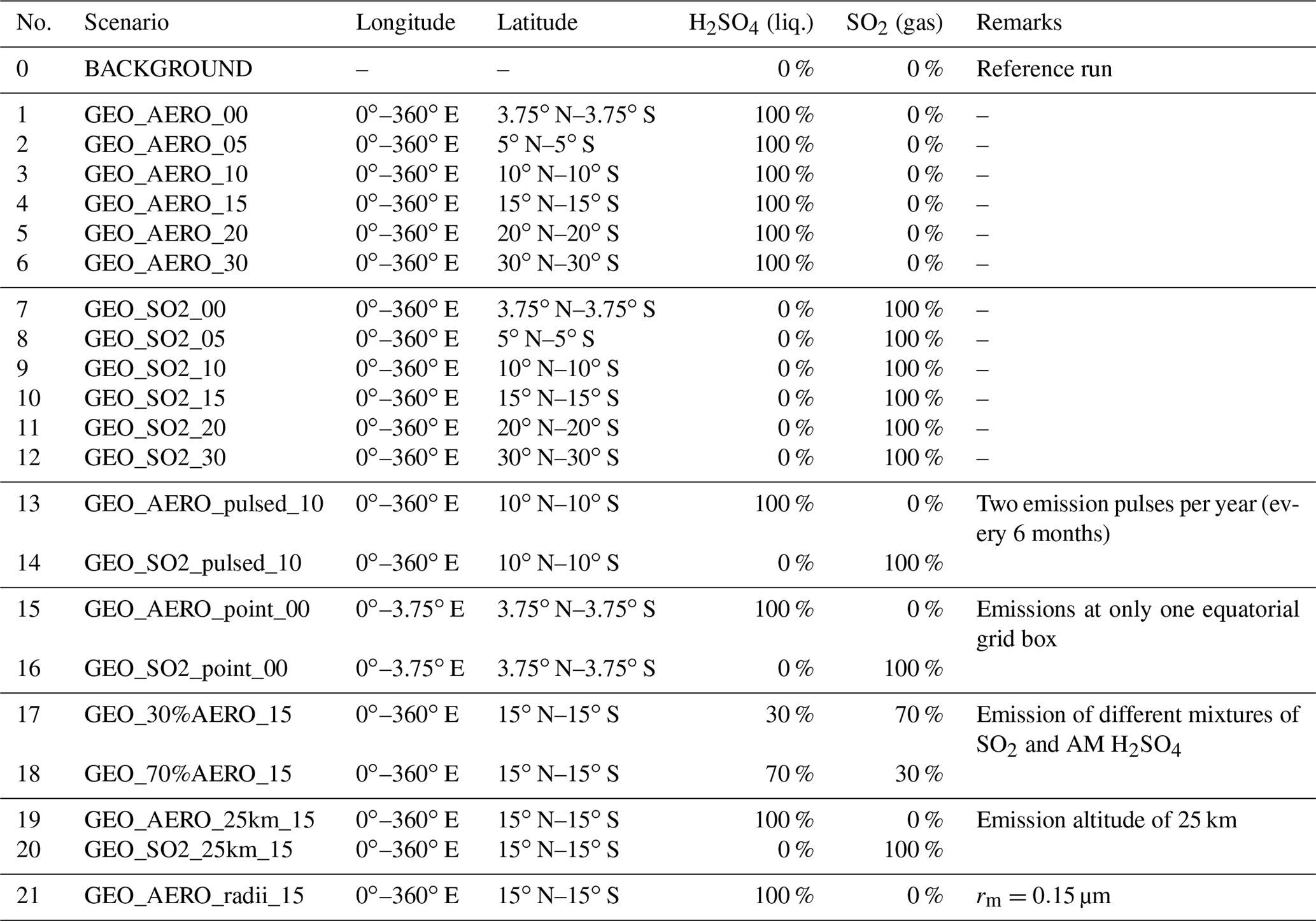
AM H₂SO₄ emissions were parameterized as a log-normal distribution with a dry mode radius (r_m) of 0.095 µm and a distribution width (σ) of 1.5. This is the resulting size distribution determined by Pierce et al. (2010) from a plume model, derived at the point when coagulation with the larger background sulfate particles became dominant over self-coagulation. We also performed one run (scenario number 21, termed “GEO_AERO_radii_15”) with a mean radius of 0.15 µm to investigate the sensitivity of aerosol burden and radiative forcing to the initial AM H₂SO₄ size distribution.

Runs 1–6 injected AM H₂SO₄ whereas runs 7–12 injected SO₂, with the respective injections in each treatment (AM H₂SO₄ or SO₂) made at the Equator (i.e., ±3.75^∘ N and S), from 5^∘ N to 5^∘ S, 10^∘ N to 10^∘ S, 15^∘ N to 15^∘ S, 20^∘ N to 20^∘ S, and from 30^∘ N to 30^∘ S, and uniformly spread over all longitudes. Emission into the tropical and subtropical stratosphere was chosen to achieve global spreading via the Brewer–Dobson circulation, and various latitudinal spreads were chosen to investigate sensitivity of emitting partly into the stratospheric surf zone and not only into the tropical pipe. The stratospheric surf zone is the region outside the subtropical transport barrier where the breaking of planetary waves leads to quasi-horizontal mixing (McIntyre and Palmer, 1984; Polvani et al., 1995). We assumed the emission to be continuous in time, and injected into one vertical model level and the indicated emission area for all the scenarios, except for scenarios 13 and 14 which emitted AM H₂SO₄ and SO₂, respectively, in two pulses per year (1–2 January and 1–2 July of every modeled year) between 10^∘ N and 10^∘ S. Runs 15 and 16 are scenarios with emissions into a single equatorial grid box (3.75^∘ × 3.75^∘ in longitude and latitude), whereas all of the other scenarios emitted equally at all longitudes around the globe. With these scenarios, we investigated differences between a point source emission such as emissions resulting from a tethered balloon, and equally spread emissions such as emissions from continuously flying planes or a dense grid of continuously operating balloons.

Figure 1 Schematic of the global sulfur cycle for GEO_AERO_15 (blue), GEO_SO2_15 (red) and BACKGROUND (black) averaged over the last 10 years of simulations (see Table 1 for scenario definitions). Net fluxes (positive in the direction of the arrows) are given in Gg S yr⁻¹ and burdens (in boxes) are given in Gg S. Species of SO₂ precursors include OCS, DMS, H₂S, and CS₂. SO₃, as an intermediate step between SO₂ and H₂SO₄, is modeled but for simplicity is omitted from the diagram.

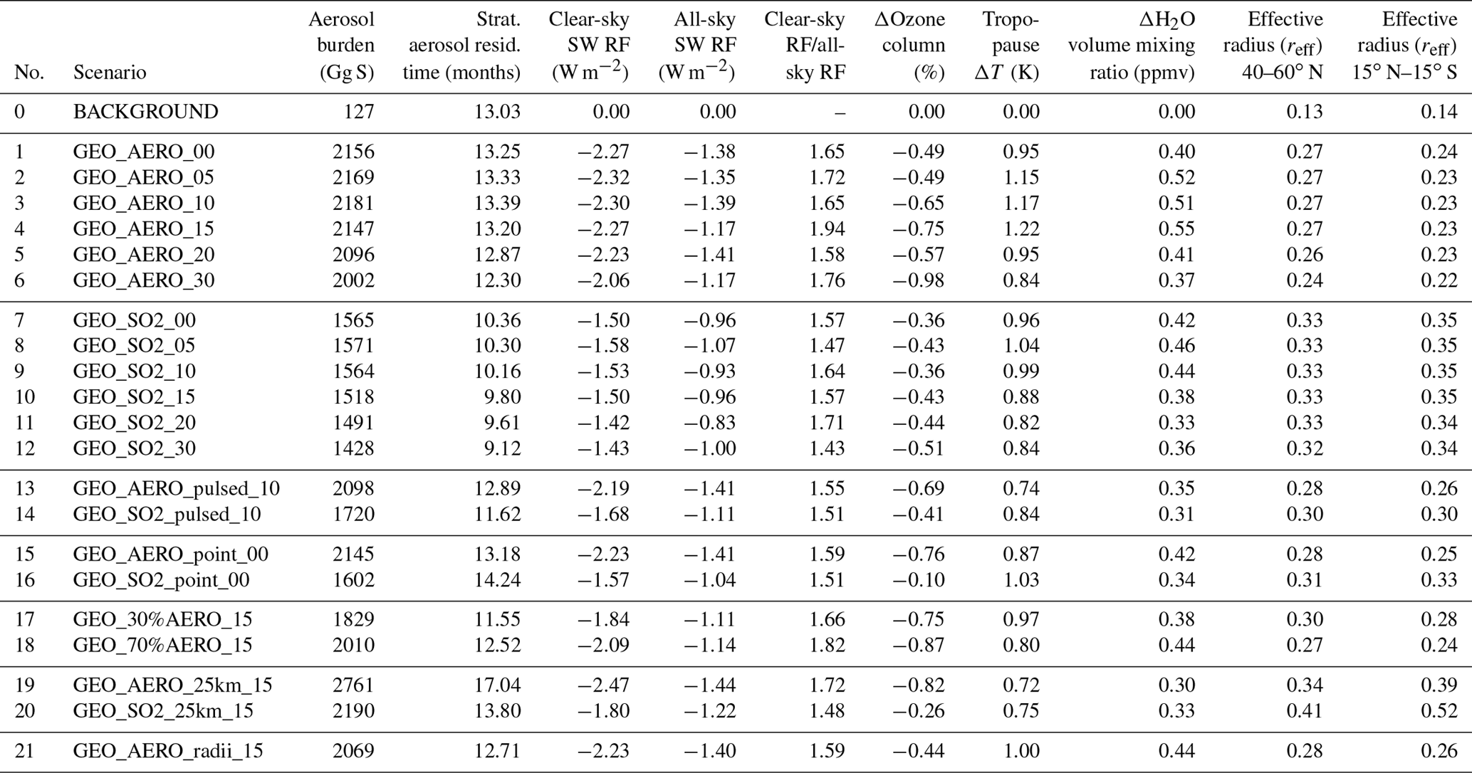
Table 2 Summarized values of all quantities calculated in this study. The first five columns show total stratospheric aerosol burden, stratospheric aerosol residence time, globally averaged clear-sky and all-sky surface shortwave (SW) radiative forcing, as well as the ratio between the globally averaged clear-sky and all-sky SW radiative forcing. For ozone depletion, globally averaged values of the total ozone column reduction are shown as a percentage. Temperature increases and H₂O volume mixing ratio increases are given as values averaged between 15^∘ N and 15^∘ S at 90 hPa (i.e., at the tropical cold point tropopause). The last two columns show wet effective radius (r_eff) averaged between 40 and 60^∘ N at 100 hPa and between 15^∘ N and 15^∘ S at 50 hPa.

We assume that AM H₂SO₄ is produced in situ in the plumes behind planes which generate SO₃ or H₂SO₄ from burning elemental sulfur. As a 100 % conversion rate is unlikely to be achieved (Smith et al., 2018), we also performed two runs emitting mixtures of SO₂ and AM H₂SO₄ with only 30 % or 70 % in the form of AM H₂SO₄ and the rest in the form of SO₂ (runs 17 and 18, respectively).

Finally, we note that a fully coupled ocean would be desirable to study impacts on tropospheric climate such as surface temperature change. For computational efficiency, we chose not to couple the deep ocean module of SOCOL-AER in the present study. Therefore, we focus on changes in stratospheric aerosol microphysics, chemistry and changes in surface radiation. We also note particular sensitivities to which the horizontal and vertical resolution may play an important role.

4 Results

4.1 The stratospheric sulfur cycle under SSG conditions

A simplified representation of the modeled stratospheric sulfur cycle is shown for background conditions and for two geoengineering scenarios in Fig. 1. Under background conditions (black numbers in figure), the stratospheric sulfur burden primarily arises from cross-tropopause net fluxes of SO₂ and SO₂ precursor species (OCS, DMS, CS₂ and H₂S) as well as primary tropospheric sulfate aerosols in the rising air masses in the tropics. OCS contributes to the SO₂ burden in the middle stratosphere, whereas the direct cross-tropopause flux of SO₂ mainly influences the lower stratosphere (Sheng et al., 2015). In the tropical stratosphere, the mean stratospheric winds disperse sulfur species readily in east–west directions, whereas meridional transport is determined by large-scale stirring and mixing through the edge of the tropical pipe at typical latitudes of 15^∘–20^∘ N and S (Plumb, 1996). Transport into higher latitudes, which occurs mainly via the Brewer–Dobson circulation (Brewer, 1949; Dobson, 1956), results in a stratospheric aerosol residence time (which is equal to the stratospheric burden divided by net flux to the troposphere) of about 13 months for background conditions in SOCOL-AER (see Table 2). After the decomposition of sulfate precursors to SO₂ and the subsequent oxidation to H₂SO₄ vapor, sulfate aerosol particles are formed via bimolecular nucleation with H₂O or grow via condensation onto preexisting aerosol particles. Condensation is proportional to the available surface area of preexisting aerosols, and nucleation is mainly a function of temperature and H₂SO₄ partial pressure. The resulting stratospheric aerosol burden differs in some details (∼16 % larger total stratospheric aerosol mass) from the one simulated in Sheng et al. (2015) due to different temporal sampling of model output as well as subsequent model updates and development.

The aerosol burden resulting from geoengineering AM H₂SO₄ injection for scenario GEO_AERO_15 (blue) is 41.4 % larger than the aerosol burden resulting from the equivalent SO₂ injection for scenario GEO_SO2_15 (red). The chemical lifetime of SO₂ in the lower stratosphere varies from 40 to 47 days among our SO₂ emission scenarios (about 31 days for background conditions). The SO₂ injection from GEO_SO2_15 results in an averaged stratospheric SO₂ burden of 222.4 Gg S for steady-state conditions, which is 12.8 % of the combined stratospheric SO₂ and aerosol burden. This is a significant fraction compared to the 0.6 % in AM H₂SO₄ emission scenarios, especially when considering that the sulfur only becomes “useful” for SSG after transformation to sulfate aerosols. In SO₂ emission scenarios only 4.7 % of the total emitted SO₂ is transported back to the troposphere unprocessed via diffusion and mixing due to tropopause folds at the edges of the tropical pipe. The other 95.3 % of the annually emitted SO₂ is subsequently oxidized to H₂SO₄ of which only 1 % is decomposed to SO₂ again via photolysis, 39 % nucleates to form new particles and 60 % condenses onto existing particles. Compared to background conditions, GEO_AERO_15 shows a shift in the processing from nucleation to condensation due to the increased surface area availability. Both SSG scenarios show an increased OCS flux across the tropopause (about +7 % among all scenarios) in comparison with the BACKGROUND run. This could be an indicator of enhanced upward mass fluxes across the tropical tropopause under SSG conditions or of decreased horizonal mixing from the tropical pipe to higher latitudes due to higher temperatures in the lower stratosphere (see Sect. 4.3) and thus modification of the Brewer–Dobson circulation as observed in Visioni et al. (2017). Table 2 lists averaged values of the aerosol burden, SW radiative forcing and other quantities for all scenarios modeled, whereas Table 3 provides the quantities normalized by the corresponding all-sky SW radiative forcing.

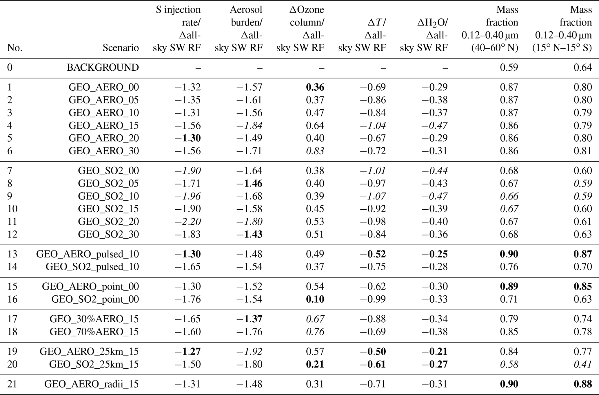
Table 3 Comparison of negative impacts investigated in this study normalized to the all-sky SW radiative forcing. The smaller the absolute value of the ratio, the smaller the injection rate or impact to achieve a given level of radiative forcing. For each of the first five columns, the three smallest/largest absolute values are marked in bold/italic. Columns show globally averaged values of the sulfur injection rate, the resulting global stratospheric aerosol burden and the ozone depletion at 50 hPa as well as H₂O volume mixing ratio increase and temperature increases at the tropical cold point tropopause (i.e., at 90 hPa) normalized to the resulting all-sky SW radiative forcing. The last two columns show the wet aerosol mass fraction in the range between 0.12 and 0.40 µm of the resulting size distribution. In the last two columns, the three largest mass fractions are marked in bold and the three smallest mass fractions are marked in italic.

The SO₂ injection case produces both more nucleation-mode (<0.01 µm radius) particles and more coarse-mode (>1 µm radius) particles than the AM H₂SO₄ case (Fig. 2). GEO_SO2_15 shows number concentrations of large particles in the coarse mode that are about 3 orders of magnitude higher than GEO_AERO_15. The concentration of tiny nucleation-mode particles is about 2–3 orders of magnitude higher compared with the BACKGROUND scenario. This is due to the large nucleation rate driven by H₂SO₄ gas formed from SO₂ oxidation in GEO_SO2_15. The increase in coarse-mode particles is partly due to H₂SO₄ condensing onto existing aerosols, and partly due to increased continuous coagulation of freshly formed nucleation-mode particles with larger particles. The larger concentration of coarse-mode particles in SO₂ emission scenarios leads to increased aerosol sedimentation rates and thus to 25.8 % shorter stratospheric aerosol residence times compared with AM H₂SO₄ emission scenarios. We also show the fifth moment of the aerosol size distribution (see Fig. 2c), which gives an estimate of the downward mass flux due to aerosol sedimentation. This shows that particles in the size range from 0.4 to 1.5 µm contribute the most to sedimentation in the GEO_SO2_15 scenario. We can explain the total difference of the 29.3 % smaller stratospheric aerosol burden in GEO_SO2_15 compared with GEO_AERO_15 by the 4.7 % of emitted SO₂ that is lost to the troposphere unprocessed and the 25.8 % shorter stratospheric aerosol residence time.

Figure 2 Size and mass distributions of stratospheric aerosol under various scenarios. (a) Wet aerosol size distributions of GEO_AERO_15 (blue), GEO_SO2_15 (red) and BACKGROUND (black) are zonally averaged over 10 years between 15^∘ N and 15^∘ S (continuous lines) and between 40 and 60^∘ N (dashed lines). Values shown are at 50 hPa in the tropics and at 100 hPa in the northern midlatitudes, i.e., at the levels of peak aerosol mass concentration in the vertical profile (see Fig. 3). The green size range is defined as the radius at which backscattering efficiency on sulfate aerosols is at least 70 % (i.e., 0.12–0.40 µm) of its maximal value (solid green line at 0.30 µm) following Dykema et al. (2016). (b) The resulting mass distributions of the size distribution curves shown in (a) including the wet aerosol mass fraction in the optimal size range between 0.12 and 0.40 µm in the legend. (c) The fifth moment of the aerosol size distribution shown in (a) as an estimate for aerosol sedimentation mass flux.

In the AM H₂SO₄ case, the number concentration of nucleation-mode particles decreases below background conditions due to the increased surface area available for condensation (see Fig. 2) and the increased coagulation of nucleation-mode particles with accumulation-mode particles. For particles larger than a radius of 10 nm, the simulated distribution in the tropics is similar to the injected aerosol distribution with a peak of about 100 particles per cm³ at a radius of about 0.1 µm. In Fig. 2, the size range between 0.12 and 0.40 µm is highlighted in green as the range in which the efficacy of backscattering solar radiation on sulfate aerosols is at least 70 % of its peak value at 0.3 µm (solid green line, Dykema et al., 2016). In the tropics, the mass fraction of particles in the 0.12 to 0.40 µm size range is 0.79 of the total tropical aerosol mass for GEO_AERO_15 and 0.60 for GEO_SO2_15 (see also Table 3). Coagulation and sedimentation during transport to higher latitudes reduces the overall particle concentration in higher latitudes (dashed curves in Fig. 2) while increasing the mean particle size. Subsequently, the peak at about 0.1 µm in the tropics in GEO_AERO_15 becomes less pronounced and shifts slightly towards larger particles, which is closer to the radius of maximal backscattering of solar radiation on sulfate aerosols. Among all scenarios, the mass fraction in the optimal size range between a radius of 0.12 and 0.40 µm increases with transport to higher latitudes (e.g., 0.86 for GEO_AERO_15 and 0.67 for GEO_SO2_15 between 40 and 60^∘ N), which results in a larger radiative forcing efficiency per unit stratospheric aerosol burden (see Fig. 2 and Table 3). Overall, AM H₂SO₄ emission scenarios result in a more favorable aerosol size distributions, with more particles in the optimal size range for backscattering solar radiation compared with SO₂ emission scenarios.

The more favorable size distribution in the AM H₂SO₄ emission scenarios is also illustrated by values of effective radius (r_eff) for different scenarios (Fig. 3 and Table 2). The effective radius is the ratio of the third moment to the second moment of the size distribution. The size range between 0.24 and 0.36 µm, which is the range at which mass specific up-scatter is at least 90 % of its peak backscattering efficiency at 0.3 µm, is marked by the stippled area in Fig. 3. In GEO_AERO_15 (Fig. 3a) this r_eff size range is seen in the lower stratosphere where aerosol mass concentrations are largest. However, GEO_SO2_15 (Fig. 3d) shows r_eff values larger than is optimal for backscattering (up to 0.40 µm) in parts of the lower stratosphere. Our values of r_eff for SO₂ emission scenarios are somewhat larger than those computed by Niemeier et al. (2011), who found effective radii of about 0.3 µm in the lower stratosphere when emitting 2 Mt S in form of SO₂ at 60 hPa and 0.35 µm when emitting at 30 hPa. This is due to the different setup of the two studies. Niemeier et al. (2011) emitted at only one equatorial model grid box. In our model, emission at one grid box also results in smaller particles with an effective radius of 0.33 µm averaged between 15^∘ N and 15^∘ S at 50 hPa (see Sect. 4.2, spatiotemporal spread of emissions).

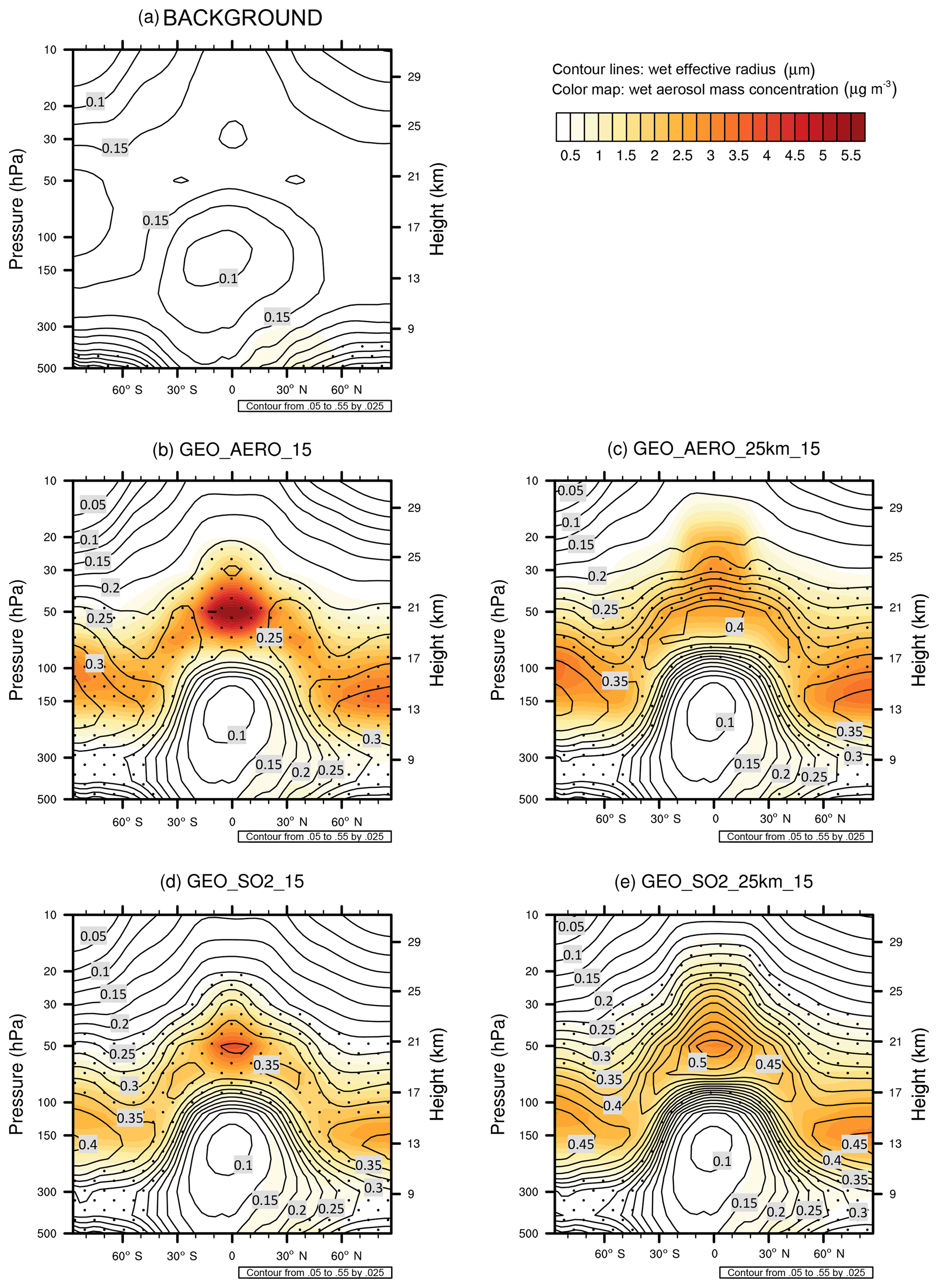
Figure 3 Contour lines show the wet effective radius (i.e., the ratio between the third moment and the second moment of the aerosol size distribution) in µm. The stippled area depicts the size range with effective radii between 0.24 and 0.36 µm. It is the range in which the backscattering efficiency is larger than 90 % of its peak value at 0.3 µm following Dykema et al. (2016). Color maps show the wet aerosol mass distribution in µg m⁻³ both zonally averaged over 10 years for background conditions (a), GEO_AERO_15 (b), GEO_AERO_25km_15 (c), GEO_SO2_15 (d) and GEO_SO2_25km_15 (e).

4.2 Sensitivity simulations

Latitudinal spread of emissions

Previous studies have found that the latitude range of emissions is important in determining size distribution and aerosol burden, and thus the resulting SW radiative forcing. English et al. (2012) found a 60 % larger aerosol burden when emitting AM H₂SO₄ between 32^∘ N and 32^∘ S when compared to emitting between 4^∘ N and 4^∘ S. They suggested that this is partly due to reduced aerosol concentrations and thus less coagulation as a result of a more dilute aerosol plume. However, they simultaneously increased the emission altitude; thus, they also stated that the increased aerosol burden could partly be due to the increased stratospheric aerosol residence time at a higher emission altitude. In contrast, Niemeier and Timmreck (2015), who only emitted at one equatorial model grid box found small decreases in aerosol burden (4.3 %) when emitting between 30^∘ N and 30^∘ S relative to emitting from 5^∘ N to 5^∘ S. They found greater coagulation with more diffuse emissions, and that emission into the stratospheric surf zone increased cross-tropopause transport of aerosols and SO₂, thus resulting in a reduced stratospheric aerosol burden compared with scenarios that only emitted SO₂ into the tropical pipe.

We find a small reduction in aerosol burden (<10 %) and clear-sky SW radiative forcing for both AM H₂SO₄ and SO₂ emission scenarios with increased latitudinal spread of the emissions (see Fig. 4). We assume that increased loss of stratospheric aerosols through tropopause folds in the surf zone with broadly spread emissions (>15^∘ N–15^∘ S) is compensated for by increased coagulation and sedimentation of aerosols in scenarios which only emit into the tropical pipe.

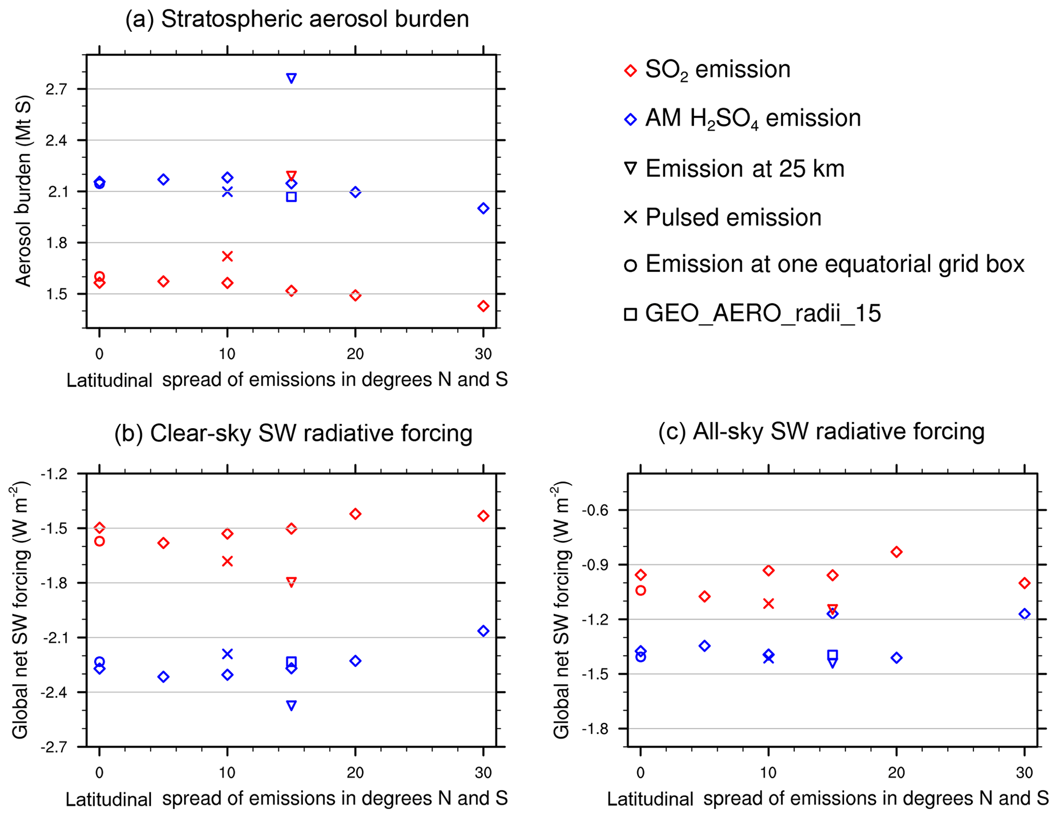
Figure 4 Globally averaged stratospheric aerosol burden (a), clear-sky (b) and all-sky (c) SW surface radiative forcing for various scenarios simulated in this study. AM H₂SO₄ emission scenarios are shown in blue and SO₂ emission scenarios are shown in red. Reference scenarios are shown using “diamond” symbols. Alternate cases are shown using the symbols indicated in key.

Sensitivity to emission altitude

The stratospheric aerosol residence time when emitting at 24 hPa (∼25 km) is increased by 28.6 % and 44.3 % when emitting AM H₂SO₄ and SO₂, respectively, relative to emitting at 50 hPa (∼20 km). Therefore, GEO_AERO_25km_15 and GEO_SO2_25km_15 result in a stratospheric aerosol burden of 2761 and 2190 Gg S, respectively. In GEO_SO2_25km_15 the loss of unprocessed SO₂ to the tropopause is reduced to 2.3 % due to the greater distance of emissions from the tropopause and higher OH concentrations with increasing altitude in the stratosphere. However, because of warmer temperatures at higher altitudes in the stratosphere, the nucleation rate decreases and a larger fraction of the H₂SO₄ gas condenses onto preexisting particles (12.4 % nucleation, 87.6 % condensation). Therefore, particles tend to grow to even larger sizes and more particles accumulate in the coarse mode. The mass fraction of particles between 0.12 and 0.40 µm is reduced to only 0.41, and the all-sky SW radiative forcing is only increased by 27.1 % in magnitude compared with GEO_SO2_15, which is not proportional to the increase in the stratospheric aerosol burden (44.3 %). For GEO_AERO_25km_15 the fraction between 0.12 and 0.40 µm is only reduced from 0.79 to 0.77. This results in an all-sky SW radiative forcing increase of 23.1 % compared with GEO_AERO_15, which is close to the increase in stratospheric aerosol burden (28.6 %). The latitudinal and vertical distribution of the aerosol mass density and the larger aerosol sizes are also seen in the values of r_eff (Fig. 3c, e). When emitting at 25 km, the r_eff in the tropical lower stratosphere increases from 0.35 to 0.52 µm in the SO₂ emission case and from 0.23 to 0.39 µm in the AM H₂SO₄ emission case. Thus, the stippled area in Fig. 3c and e (r_eff of 0.24 to 0.36 µm) is below and above the lower stratosphere where most aerosol mass is accumulated. Therefore, emitting at 25 km results in less SW radiative forcing per resulting stratospheric aerosol burden. Furthermore, aerosol density remains more concentrated in the tropics when emitting at 25 km (see also Fig. 7a, b), due to a less leaky tropical pipe at higher stratospheric altitudes. However, when looking at the resulting clear-sky SW radiative forcing (Fig. 7c, d), the peak in the tropics is only slightly increased in the SO₂ emission case and is even lower than the equivalent emission scenario at 20 km in the AM H₂SO₄ emission case.

Sensitivity to the injection mode radius

GEO_AERO_radii_15 released AM H₂SO₄ with mean radii of 0.15 µm instead of 0.095 µm. This results in slightly fewer but larger particles in the emitted aerosol plume. The increased injection radius resulted in a slightly reduced aerosol burden due to either different coagulation and condensation regimes or faster sedimentation of the slightly larger particles. However, due to the increase of particles in the optimal size range for backscattering solar radiation (+11.4 %), the all-sky SW radiative forcing increased by 19.7 % compared with GEO_AERO_15 (see Fig. 4). When looking at Tables 2 and 3, there is only a small difference in r_eff between the AM H₂SO₄ emission scenarios with r_m values of 0.095 and 0.15 µm, indicating only minor dependence of small changes in r_m on the resulting distribution of accumulation-mode particles.

Mixtures of AM H₂SO₄ and SO₂

We also performed calculations to explore the utility of emitting SO₂ and AM H₂SO₄ together (see Fig. 5). Some studies have suggested that planes carrying elemental sulfur and burning it in situ to directly emit H₂SO₄ gas or AM H₂SO₄ would be the most effective way to deliver sulfate to the stratosphere (Benduhn et al., 2016; Smith et al., 2018). Burning elemental sulfur would also reduce the freight to be transported to the stratosphere (i.e., 32 g mol⁻¹ for sulfur rather than 98 g mol⁻¹ for H₂SO₄ or 64 g mol⁻¹ for SO₂). However, 100 % conversion to H₂SO₄ is unlikely, with the remainder emitted as SO₂. Our results show that compared to the pure AM H₂SO₄ emission scenario GEO_AERO_15, a 30 % portion of SO₂ in the emission mixture (i.e., GEO_70%AERO_15) only leads to a slight reduction in the resulting stratospheric aerosol burden (−6.4 %) as well as in the mass fraction in the optimal size range for backscattering solar radiation and SW radiative forcing (see Tables 2 and 3); furthermore, a 30 % portion of AM H₂SO₄ in an emission mixture dominated by SO₂ (i.e., GEO_30%AERO_15) can increase stratospheric aerosol burden and SW radiative forcing significantly with respect to a pure SO₂ emission scenario (GEO_SO2_15). As the decrease in efficiency with increasing SO₂ portion in the emission mixture is strongly nonlinear in our simulations, we do not expect a significant efficiency loss for small portions of SO₂ in the emissions after in situ burning of elemental sulfur in planes.

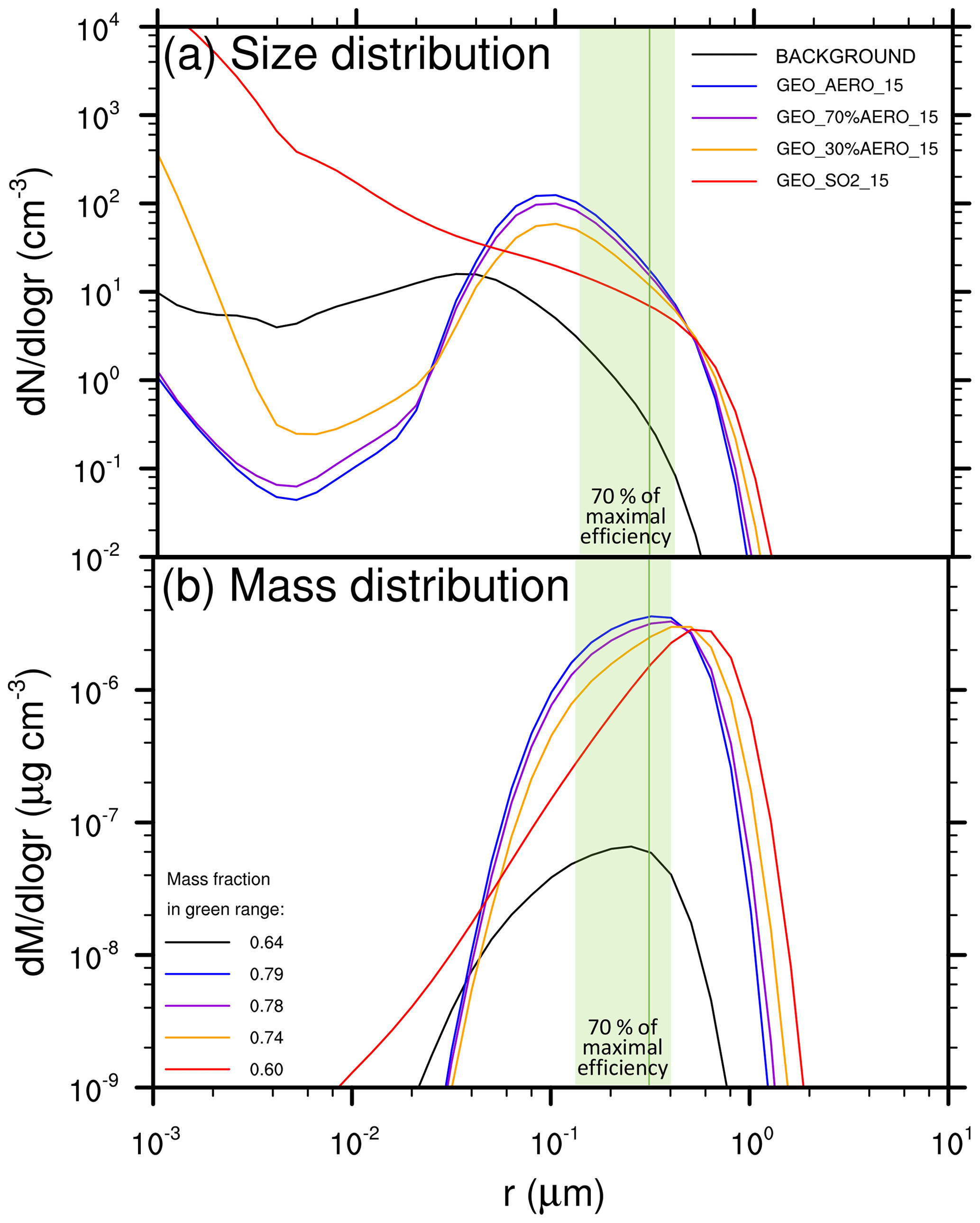
Figure 5 (a) Wet aerosol size distribution of scenarios with various emission mixtures of AM H₂SO₄ and SO₂ averaged between 15^∘ N and 15^∘ S at 50 hPa. The green size range is defined as the radius at which backscattering efficiency on sulfate aerosols is larger than 70 % (i.e., 0.12–0.40 µm) of its maximal value (solid green line at 0.30 µm) following Dykema et al. (2016). (b) Mass distributions of the size distributions resulting from (a) including the wet aerosol mass fraction in the optimal size range between 0.12 and 0.40 µm in the legend.

Spatiotemporal spread of emissions

Emitting AM H₂SO₄ in two pulses per year as assumed in GEO_AERO_pulsed_10 decreases the stratospheric aerosol burden by 3.8 % compared with the continuous emission scenario, GEO_AERO_10. This is due to the ∼91 times larger aerosol mass concentration in the emission plume compared with GEO_AERO_10 (emission during 4 days per year instead of 365), and thus more coagulation and faster sedimentation in the emission region. Similar, but smaller effects were observed for GEO_AERO_point_00, which only emitted at one equatorial grid box (3.75^∘ × 3.75^∘), and thus with 96 times the mass concentration in the emission region compared with GEO_AERO_00 (emissions spread over 3.75^∘ in longitude instead of 360^∘). This indicates fast zonal mixing which reduces the effect of the higher initial mass concentration compared with the pulsed emissions. Changes in clear-sky radiative forcing are about proportional to the aerosol burden, resulting in slightly smaller values for the sensitivity runs. However, all-sky SW radiative forcing is slightly larger compared with continuous scenarios emitting at all longitudes. This indicates aerosol size distributions with more particles in the optimal size range (see Table 3), and thus more effective backscattering of solar radiation.

However, looking at GEO_SO2_pulsed_10 and GEO_SO2_point_00, which are the equivalent SO₂ emission scenarios, the stratospheric aerosol burden increased by 10.0 % and 2.4 %, respectively, compared with the continuous emission scenarios at all longitudes. This is mainly due to a reduction in the total globally averaged aerosol nucleation rate (24.1 % nucleation, 75.9 % condensation) and the subsequent reduction in total coagulation. However, locally for GEO_SO2_point_00 and spatially for GEO_SO2_pulsed_10, the nucleation rates are increased in the emission area due to the greatly increased H₂SO₄ concentration in the emission region in these scenarios. These two scenarios produce spatially/temporally large amounts of nucleation-mode particles which then quickly coagulate to produce accumulation-mode particles. After dilution when nucleation is small again, the continuous flow of tiny, freshly nucleated particles is disrupted, and coagulation is reduced. Thus, the mean particle diameter is smaller and the stratospheric aerosol residence time is increased compared with the respective continuous emission scenarios. Due to the decrease in particle diameter and thus more particles in the optimal size range (see Table 3) the all-sky SW radiative forcing increases disproportionally compared with the stratospheric aerosol burden. All-sky SW radiative forcing is increased by 19.4 % and 8.3 % in GEO_SO2_pulsed_10 and GEO_SO2_point_00 compared with GEO_SO2_00 and GEO_SO2_00, respectively (see Table 2). This partially mimics the processes in an SO₂ plume emitted by an aircraft. Other models also found single grid box SO₂ emissions to result in more effective radiative forcing (Niemeier et al., 2011) or found no difference compared to emissions at all longitudes (English et al., 2012). However, the different behavior between point/pulsed SO₂ and point/pulsed AM H₂SO₄ emission scenarios, which may be similar to solid aerosol particles, is novel and has never been shown before.

4.3 Temperature, OH, H₂O and methane at the tropical cold point tropopause

Increased aerosol burden in the stratosphere also leads to heating of the lower stratosphere, mainly due to absorption of longwave radiation. Heating of the cold point tropopause results in temperature increases of 0.7–1.2 K among all scenarios, associated with a H₂O entry value increase of 0.30–0.55 ppmv (i.e., 9 %–17 %, see Fig. 6 and Table 2). The increased stratospheric H₂O volume mixing ratio results in an increase of the OH volume mixing ratio (H₂O+O(¹D) $=>\mathrm{2}$ OH), which additionally increases the HO_x ozone depletion cycle.

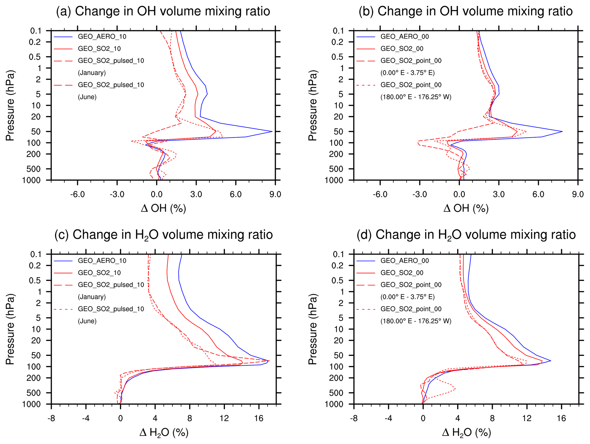
Figure 6 Vertical profile of the OH volume mixing ratio anomaly (a) and (b), and H₂O volume mixing ratio anomaly (c) and (d). Anomalies represent prudential difference compared with the BACKGROUND simulation. Data show annual and zonal averages between 15^∘ N and 15^∘ S except where indicated. The left column, (a) and (c), shows results for injections within 10^∘ of the Equator, whereas the right column, (b) and (d), shows results for injections at the Equator. For equatorial injections ((b), (d)), we show results averaged from 0 to 3.75^∘ E and from 180^∘ E to 176.25^∘ W. For the 10^∘ injection case ((a), (c)), we show zonal averages for January (emissions during 1 and 2 January) and June (month before emission) from the pulsed simulation. Note how SO₂ injection scenarios tend to reduce OH concentrations around 50 hPa compared with AM H₂SO₄ injection scenarios (due to the reaction SO₂+OH$=>$ SO₃+HO₂), whereas both increase stratospheric H₂O concentrations due to warming.

Figure 6c and d show how the H₂O volume mixing ratios increase above 200 hPa. The increase is slightly larger for the AM H₂SO₄ scenarios due to the higher aerosol load and more pronounced heating of the lower stratosphere. However, when comparing the vertical OH profiles (Fig. 6a, b), the difference in OH between the SO₂ and the AM H₂SO₄ scenarios increases to about 4 % at approximately 50 hPa, which is caused by the depletion of OH due to SO₂ oxidation (SO₂+OH $=>$ SO₃+HO₂).

Kleinschmitt et al. (2018) applied a mean lifetime of 41 days for SO₂ to H₂SO₄ conversion in their study and found a SO₂-to-H₂SO₄ conversion rate of 96 %. They expected a slightly lower concentration in oxidants and therefore a longer SO₂ lifetime as well as a lower SO₂-to-H₂SO₄ conversion rate when taking chemical interactions into account. However, they did not consider the increased stratospheric H₂O volume mixing ratio under SSG conditions which causes an OH concentration increase of up to 9 % in our model, making the stratospheric SO₂ lifetime shorter and the SO₂-to-H₂SO₄ conversion rate larger.

There are other side effects of SSG such as a tropospheric methane lifetime increase. In our simulation, tropospheric methane mixing ratios remain largely unchanged as we use prescribed mixing ratio boundary conditions for methane at the ground as well as prescribed SST. However, the reaction of methane with OH is strongly temperature dependent. In our model we observe a tropospheric temperature decrease of up to 0.95 K which leads to an increase in the methane lifetime of up to 2.3 %, whereas OH concentration is almost unchanged in our simulations. Therefore, our model shows a similar effect as in Visioni et al. (2017), although much smaller, as we only emitted 1.83 Mt S per year and Visioni et al. (2017) emitted 5 Mt S per year. When we scale our results linearly to 5 Mt S per year, the methane lifetime increases by up to 6.3 % depending on the scenario. This is still less then the 10 % found by Visioni et al. (2017), probably due to the constant SST in our model setup. When taking interactive SST into account, increased changes in temperature, tropospheric ozone and O¹(D) chemistry as well as H₂O concentrations could account for the remaining difference with respect to Visioni et al. (2017). In our simulations, the lifetime of methane at 50 hPa in the lower stratosphere decreases by about 14 % in continuous AM H₂SO₄ emission scenarios at all longitudes and by about 10 % in the corresponding SO₂ emission scenarios, which is in agreement with the OH changes described above.

4.4 AM H₂SO₄ versus SO₂ emissions

All-sky SW radiative forcing from AM H₂SO₄ emission scenarios 1–6 result in an average of 1.31 W m⁻². This value is 36.5 % larger than the average of the equivalent SO₂ emission scenarios 7–12, which result in 0.96 W m⁻². For clear-sky SW radiative forcing the AM H₂SO₄ scenarios 1–6 are roughly 50 % higher on average then SO₂ emission scenarios 7–12. Table 2 summarizes globally averaged quantities of all modeled SSG scenarios. The fifth column shows the ratios between surface clear-sky and surface all-sky SW radiative forcing. These values for the AM H₂SO₄ emission scenarios are about 10 % higher than for the SO₂ emission scenarios, indicating a larger reduction of SW radiative forcing due to clouds and/or chemical interactions among AM H₂SO₄ scenarios. The stratospheric aerosol burdens for the AM H₂SO₄ scenarios are more concentrated within the tropical pipe between 15^∘ N and 15^∘ S compared with the equivalent SO₂ emission scenarios, which are more evenly distributed across all latitudes (as shown in Fig. 7a and b). When looking at the clear-sky SW radiative forcing (Fig. 7c, d), the tropical peak flattens out compared with the peak in aerosol burden (Fig. 7a, b) because the up-scattered fraction of solar radiation increases with increasing solar zenith angle. Additionally, in higher latitudes the aerosol size distributions show more particles in the optimal size range (green ranges in Fig. 2) for backscattering solar radiation, which also leads to increased backscatter efficiency per unit stratospheric aerosol burden. For the SO₂ emission scenarios, the clear-sky SW radiative forcing is almost equally distributed between 60^∘ N and 60^∘ S, whereas for the AM H₂SO₄ scenarios, a pronounced peak can still be observed in the tropics where cloud cover is larger on average. Thus, the higher aerosol mass fraction in the cloudy tropics makes SSG less efficient in these regions. We assume the difference in surface clear-sky to surface all-sky SW radiative forcing ratios to be a result of a more favorable global spread of the resulting stratospheric aerosol burden for SO₂ emission scenarios. However, this indicates that emitting only within the tropical pipe region might not be the optimal setup for SSG studies. Emitting at the edges of the tropical pipe at 15^∘ N and 15^∘ S as investigated by Tilmes et al. (2017) might be a more efficient way to achieve higher SW radiative forcing.

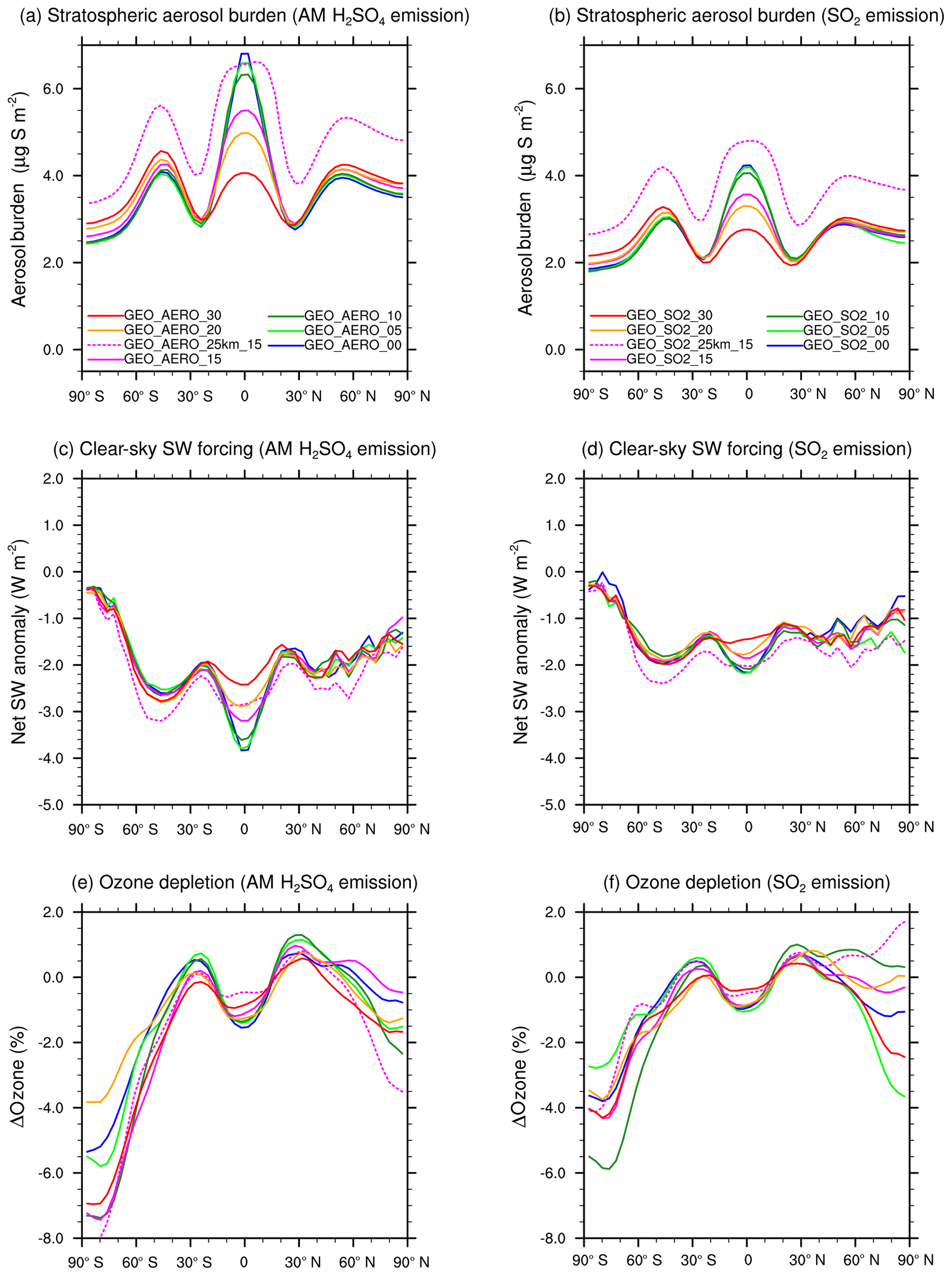
Figure 7 Zonally averaged stratospheric aerosol burden (a) and (b), clear-sky SW radiative forcing (c) and (d), and depletion of the total ozone column (e) and (f) as a function of latitude for AM H₂SO₄ (a), (c), and (e) and SO₂ (b), (d), and (f) emission scenarios with different latitudinal spread as well as for emissions at 25 km for comparison.

When looking at the depletion of the total ozone column (Fig. 7e, f), we find larger depletion among the AM H₂SO₄ emission scenarios. This is mainly due to the larger surface area densities for AM H₂SO₄ scenarios in the emission region in the tropics where ozone is produced. This leads to larger ozone depletion and thus less ozone transport to higher latitudes. Therefore, among the AM H₂SO₄ emissions scenarios, the vertical ozone column is depleted by up to 7.5 % (for GEO_AERO_15 and GEO_AERO_00) at the south polar region in a 10-year average, whereas for the SO₂ emission scenarios, it is only depleted by up to 6 % (for GEO_SO2_10). The ozone depletion arises via the formation of the reservoir species HNO₃ through N₂O₅ hydrolysis on aerosol surfaces which indirectly enhances the ClO_x ozone depletion cycle. Furthermore, chlorine becomes activated via the heterogenous reaction of ClONO₂ with HCl, which contributes the most to the ozone depletion due to SSG.

Table 3 shows values from Table 2 normalized to the globally averaged all-sky SW radiative forcing. The smallest absolute values are marked in green and the largest are marked in red. The smaller the absolute values, the larger the SW radiative forcing, and/or the smaller the negative side effects investigated in this study. Other potential negative side effects such as tropospheric cloud feedbacks (Visioni et al., 2018b) were not investigated in this study. Green values are accumulated among the AM H₂SO₄ emission scenarios and red values are accumulated among the SO₂ emission scenarios. On average, water vapor increase at the tropical cold point tropopause and global depletion of the ozone column are 15.5 % and 55.3 % larger, respectively, for AM H₂SO₄ emission scenarios 1–6 compared with SO₂ emission scenarios 7–12 when normalizing to the emission rate of 1.83 Mt S yr⁻¹. However, when normalized by the resulting all-sky SW radiative forcing, the increase in efficiency among the AM H₂SO₄ emission scenarios outweighs the worse side effects of the AM H₂SO₄ scenarios.

5 Discussion

In this study, the SOCOL-AER 3-D global aerosol–chemistry–climate model was used to investigate AM H₂SO₄ and SO₂ emission scenarios for the purpose of SSG. We analyzed the stratospheric sulfur cycle, aerosol burden, SW radiative forcing and stratospheric temperature–H₂O–OH interactions for various SSG scenarios with injections at an altitude of about 50 hPa (≈20 km) and two with injections at an altitude of about 20 hPa (≈25 km) with a sulfur mass equivalent emission rate of 1.83 Mt S yr⁻¹ within the tropics and subtropics.

Direct continuous emission of aerosol particles in the accumulation mode at all longitudes and at an altitude of 20 km results in a 37.8 %–41.4 % and a 17.0 %–69.9 % larger stratospheric aerosol burden and all-sky SW radiative forcing, respectively, compared to sulfur mass equivalent SO₂ emission scenarios. The difference in stratospheric aerosol burden is mainly due to two reasons:

1. AM H₂SO₄ emissions have the advantage of demonstrating effects immediately after emission and not only after more than 1 month of transport, photochemistry and aerosol formation as in the case of SO₂ emissions (lifetime of SO₂ of 40 to 47 days through oxidation). Thus, direct AM H₂SO₄ emission can create an immediate, targeted effect over the area of emission, whereas in SO₂ emission scenarios 12.8 % of the annually emitted sulfur is present in form of SO₂ on average.

2. The size distribution of SO₂ emission scenarios shows coarse-mode particle concentrations which are about 3 orders of magnitude larger than AM H₂SO₄ emission scenarios. These particles sediment faster and reduce the average stratospheric residence time of the aerosols compared with AM H₂SO₄ scenarios. In addition, the radiative forcing in SO₂ emission scenarios is influenced by the smaller mass fraction of particles in the optimal size range for backscattering solar radiation (i.e., 0.3 µm radius). The unfavorable size distribution for sulfate aerosols resulting from SO₂ emissions is largely due to condensation onto existing particles and the pronounced formation of tiny nucleation-mode particles which subsequently coagulate with larger aerosols to create coarse-mode particles.

The stratospheric aerosol burden and SW radiative forcing are about 10 % higher for scenarios which avoid emitting into the stratospheric surf zone, i.e., outside 15^∘ N and 15^∘ S. Enhanced loss of sulfur across the tropopause in scenarios emitting outside the tropical pipe is almost compensated for by increased coagulation and thus sedimentation in scenarios which only emit into the tropical pipe. AM H₂SO₄ emission scenarios additionally show a higher stratospheric aerosol mass fraction in the tropics. This reduces all-sky SW radiative forcing efficiency compared to SO₂ emission scenarios due to the higher cloud fraction in the tropics. The aerosol burden resulting from SO₂ emission scenarios are more equally spread to higher latitudes where an increased up-scatter fraction and a slightly better aerosol size distribution results in larger radiative forcing efficiencies per stratospheric aerosol burden. AM H₂SO₄ emission scenarios result in slightly more stratospheric ozone depletion and stratospheric warming. However, due to the larger absolute SW radiative forcing, the negative side effects investigated in this study (i.e., stratospheric ozone and methane depletion, stratospheric temperature, and H₂O increase) are smaller for AM H₂SO₄ emission scenarios than for SO₂ emission scenarios when normalizing to the surface all-sky SW radiative forcing.

On the one hand, for AM H₂SO₄ emission scenarios, temporally and spatially increasing the mass density in the emission region leads to slightly shorter aerosol residence times via more coagulation. However, all-sky SW radiative forcing is slightly increased due to the presence of slightly more particles in the optimal size range for backscattering solar radiation. On the other hand, for SO₂ emission scenarios, a larger stratospheric aerosol burden for a fixed sulfur emission rate can be achieved by temporally or spatially increasing the SO₂ mass density. This strategy increases nucleation and coagulation rates in the emission region while minimizing nucleation and coagulation on a global scale, as first shown in Niemeier et al. (2011). The optimal frequency of the pulses as well as the optimal spatial extent of the emissions requires further investigation. However, our results show different behavior of AM H₂SO₄ and SO₂ emission scenarios to temporal and spatial spreads of the emissions. They also hint at a possible dependence on small-scale processes such as locally changing SO₂ and OH mass concentrations, which cannot be resolved in GCMs. This can be important when injecting emissions along the trajectory of an aircraft. Furthermore, the results underline the importance of interactions between chemistry and aerosols when modeling SSG scenarios.

We found that in the lower stratosphere OH concentrations are increased by up to 8.8 % for AM H₂SO₄ emission scenarios compared with the BACKGROUND run due to increased temperatures at the tropical cold point tropopause and thus higher water volume mixing ratios in the stratosphere. However, due to oxidation of SO₂ in SO₂ emission scenarios, the OH concentration increase is reduced to 4 %–5 % in the lower stratosphere compared with the BACKGROUND run in these scenarios.

We also examined scenarios in which mixtures of SO₂ and AM H₂SO₄ were emitted. Pure AM H₂SO₄ emission scenarios resulted in the largest stratospheric aerosol burdens as well as the largest clear-sky and all-sky SW radiative forcing. While the SW radiative forcing decreases with increasing fractions of SO₂, the increase is nonlinear. A small fraction of SO₂ within emissions of AM H₂SO₄ results in only slightly smaller radiative forcing efficiency, whereas a small fraction of AM H₂SO₄ within emissions of SO₂ increases radiative forcing efficiency significantly. In situ burning of elemental sulfur in planes with subsequent conversion to SO₃ and, in the plume to AM H₂SO₄ particles might therefore be effective in controlling the aerosol size distribution, even if conversion efficiency were significantly less than unity.

We found clear-sky SW radiative forcing efficiencies of −1.22 and −0.82 W m⁻² per emitted megaton of sulfur equivalent injection rate (W m⁻² (Mt S yr${}^{-\mathrm{1}}{)}^{-\mathrm{1}})$ for GEO_AERO_point_00 and GEO_SO2_point_00, respectively. For all-sky SW radiative forcing, the efficiencies were −0.77 and −0.57 W m⁻² per emitted megaton of sulfur, respectively. These values for point emission scenarios are somewhat smaller compared to other models such as MAECHAM5 in Niemeier et al. (2011) and LMDZ-S3A in Kleinschmitt et al. (2018), who both reported −0.60 W m⁻² (Mt S yr${}^{-\mathrm{1}}{)}^{-\mathrm{1}}$ when emitting SO₂ into one model grid box at an altitude of 19 km and 17 km, respectively. This is likely due to differences in transport processes as well as lower stratospheric aerosol burdens in our model. On the one hand, this could partially be the result of different sedimentation, coagulation and aerosol binning schemes compared with other aerosol modules. On the other hand, SOCOL-AER slightly overestimates the Brewer–Dobson circulation (Dietmüller et al., 2018) when considering reference scenarios from the Chemistry–Climate Model Initiative (CCMI). Even though stratospheric heating by SSG is not considered there, this could result in larger aerosol burdens compared with other models. When emitting SO₂ at an altitude of 25 km the efficiency is −0.67 W m⁻² (Mt S yr${}^{-\mathrm{1}}{)}^{-\mathrm{1}}$ in SOCOL-AER (emissions at all longitudes) and −0.80 W m⁻² (Mt S yr${}^{-\mathrm{1}}{)}^{-\mathrm{1}}$ in MAECHAM5 (Niemeier et al., 2011, with emissions at one grid box at 24 km). This is not proportional to the increase in the stratospheric aerosol burden which is due to less favorable size distributions for backscattering solar radiation in these scenarios (see Sect. 4.2, sensitivity to emission altitude). However, as many processes are nonlinear with increasing injection rates and altitudes, the efficiencies might be different for other SSG setups. Due to the lack of atmospheric observations or small-scale field experiments, modeling studies are currently the only method to estimate the efficiency and the possible adverse effects of SSG. Therefore, model intercomparison studies should further identify strengths and weaknesses among different models to reduce uncertainty. Furthermore, atmospheric field studies such as the Stratospheric Controlled Perturbation Experiment (SCoPEx, Dykema et al., 2014) could give further insight into stratospheric aerosol formation and plume evolution.

Additional uncertainties arise from the rather low resolution applied in this study. In particular, an increase in the vertical resolution as well as the treatment of an interactive QBO could further increase the explanatory power of SSG studies using SOCOL-AER. To study tropospheric climate change, ocean feedback would have to be taken into account with the deep ocean module of SOCOL-AER. Furthermore, SOCOL-AER does not treat cloud interactions – which is likely one of the major uncertainties of the model, as aerosols may have large impacts on clouds (Kuebbeler et al., 2012; Visioni et al., 2018b). We only performed scenarios with emission regions limited to the tropics and subtropics centered around the Equator. Nevertheless, SOCOL-AER is one of the first models that interactively couples a sectional aerosol module to the well-described chemistry and radiation schemes of a CCM.

This study shows that direct emission of aerosols can give better control of the resulting size distribution, which subsequently results in more effective radiative forcing. Therefore, the SSG modeling community should increase their focus on direct AM H₂SO₄ emission as well as on the emission of solid particles (Weisenstein et al., 2015), such as calcite particles (Keith et al., 2016). Further investigations using SOCOL-AER to understand the adverse effects of SSG, such as a closer look at ozone depletion, impacts on precipitation patterns or impacts on stratospheric dynamics will be conducted in future studies. These studies will also include coupling of the deep ocean module of SOCOL-AER to investigate impacts on the tropospheric climate.

Furthermore, we show that interactive coupling of aerosols, chemistry and radiation schemes are essential features for modeling SSG emission scenarios with GCMs. For SO₂ emission scenarios, local depletion of oxidants was found, particularly with large SO₂ mass concentrations in the emission region. Accurate modeling of these scenarios might require higher temporal and spatial resolution than has been achieved with current GCMs. Therefore, coupling of small-scale Lagrangian plume dispersion models which simulate the first few days of aerosol–chemistry interactions and aerosol microphysics in evolving emission plumes from aircraft might be a desirable tool to improve future SSG modeling studies. This would appropriately account for the problem of connecting small-scale temporal and spatial processes – such as aerosol formation, growth and evolution in an aircraft wakes – to the larger grid of GCMs, which has been neglected in past SSG studies.