BVOC–aerosol–climate feedbacks investigated using NorESM

Both higher temperatures and increased CO₂ concentrations are (separately) expected to increase the emissions of biogenic volatile organic compounds (BVOCs). This has been proposed to initiate negative climate feedback mechanisms through increased formation of secondary organic aerosol (SOA). More SOA can make the clouds more reflective, which can provide a cooling. Furthermore, the increase in SOA formation has also been proposed to lead to increased aerosol scattering, resulting in an increase in diffuse radiation. This could boost gross primary production (GPP) and further increase BVOC emissions. In this study, we have used the Norwegian Earth System Model (NorESM) to investigate both these feedback mechanisms. Three sets of experiments were set up to quantify the feedback with respect to (1) doubling the CO₂, (2) increasing temperatures corresponding to a doubling of CO₂ and (3) the combined effect of both doubling CO₂ and a warmer climate. For each of these experiments, we ran two simulations, with identical setups, except for the BVOC emissions. One simulation was run with interactive BVOC emissions, allowing the BVOC emissions to respond to changes in CO₂ and/or climate. In the other simulation, the BVOC emissions were fixed at present-day conditions, essentially turning the feedback off. The comparison of these two simulations enables us to investigate each step along the feedback as well as estimate their overall relevance for the future climate.

We find that the BVOC feedback can have a significant impact on the climate. The annual global BVOC emissions are up to 63 % higher when the feedback is turned on compared to when the feedback is turned off, with the largest response when both CO₂ and climate are changed. The higher BVOC levels lead to the formation of more SOA mass (max 53 %) and result in more particles through increased new particle formation as well as larger particles through increased condensation. The corresponding changes in the cloud properties lead to a −0.43 W m⁻² stronger net cloud forcing. This effect becomes about 50 % stronger when the model is run with reduced anthropogenic aerosol emissions, indicating that the feedback will become even more important as we decrease aerosol and precursor emissions. We do not find a boost in GPP due to increased aerosol scattering on a global scale. Instead, the fate of the GPP seems to be controlled by the BVOC effects on the clouds. However, the higher aerosol scattering associated with the higher BVOC emissions is found to also contribute with a potentially important enhanced negative direct forcing (−0.06 W m⁻²). The global total aerosol forcing associated with the feedback is −0.49 W m⁻², indicating that it has the potential to offset about 13 % of the forcing associated with a doubling of CO₂.

1 Introduction

Our climate is warming due to rising atmospheric levels of greenhouse gases originating from human activities (IPCC, 2013). Feedback mechanisms that arise from increasing temperatures and/or greenhouse gas concentrations can enhance or dampen the temperature increase, and contribute to the overall uncertainty in predicting the future climate. Increased emissions of biogenic volatile organic compounds (BVOCs) from terrestrial vegetation caused by increasing temperature and CO₂ levels have been proposed to induce a negative climate feedback (Kulmala et al., 2004, 2013). Higher BVOC concentrations result in higher aerosol number and mass concentration, which cool the climate by inducing changes in cloud properties (Twomey, 1974; Albrecht, 1989). Aerosol particles and their interactions with clouds and climate constitute one of the largest uncertainties in assessing our future climate (IPCC, 2013).

BVOCs are important sources of aerosol particles (Glasius and Goldstein, 2016), especially in pristine forest regions (Tunved et al., 2006). The most important BVOC compounds for aerosol formation are isoprene, monoterpenes and sesquiterpenes (Kulmala et al., 2013), and their emissions have been estimated to be 700–1000 Tg C annually (Laothawornkitkul et al., 2009). Through oxidation in the atmosphere, these compounds become less volatile and may contribute to aerosol formation. The main oxidation agents are OH, O₃ and NO₃ radicals (Shrivastava et al., 2017). The oxidation products from monoterpenes have been found to be particularly important for new particle formation, while the oxidation products from isoprene have been found to predominantly participate in condensation onto pre-existing aerosols (Jokinen et al., 2015). How sensitive the aerosol number concentration is to changes in BVOC emissions depends on the anthropogenic and natural aerosol load. It has been shown that the BVOCs had greater influence on the number and mass concentration in the pre-industrial (PI) atmosphere (Gordon et al., 2017). The importance of new particle formation and condensation from organic vapours to the global aerosol load, cloud formation and climate has been getting increasing attention over the past 10 years (Glasius and Goldstein, 2016). However, there are still large uncertainties associated with these processes and this contributes to the overall uncertainty of aerosol particles' impact on climate (Kulmala et al., 2013).

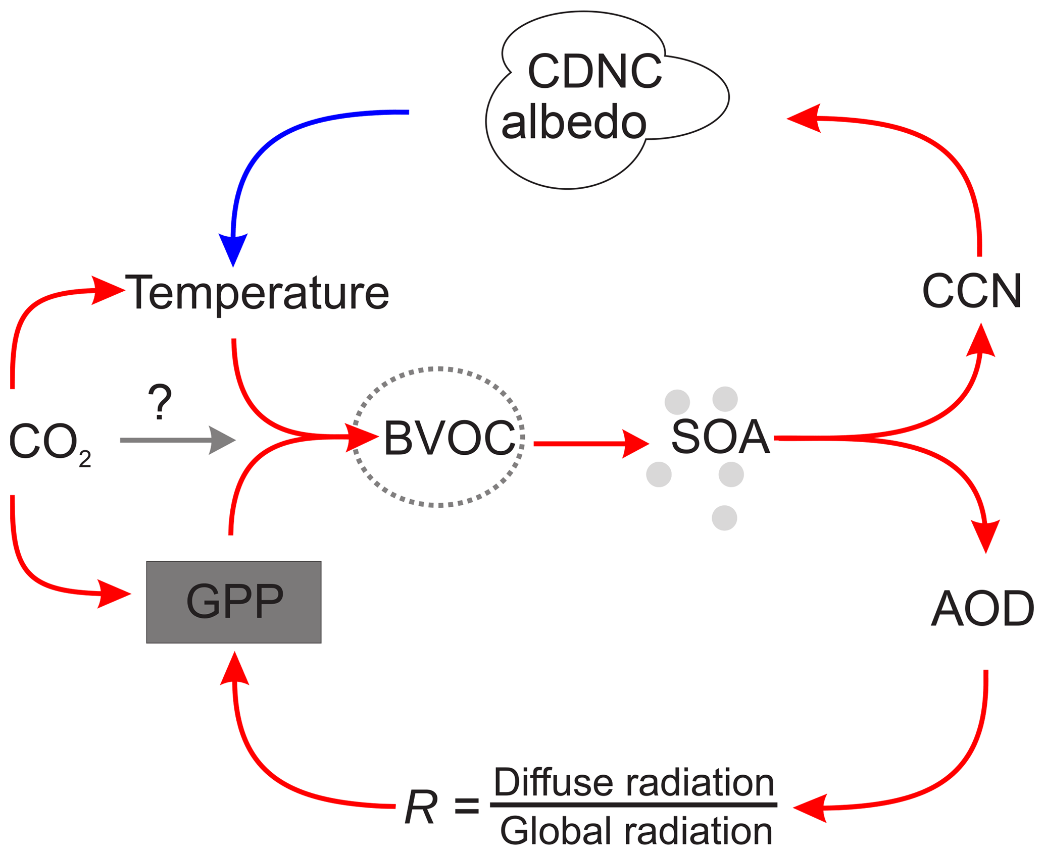
Figure 1 The BVOC feedback driven by increasing CO₂ and temperature. The upper branch of the feedback is the T branch, while the lower part is the GPP branch. The red arrows in the figure indicate that if the variable at the start of the arrow increases, then the variable at the end of the arrow is also expected to increase. A blue arrow on the other hand means that an increase in the variable at the start of the arrow is expected to result in a decrease in the variable at the end of the arrow. The figure is modified after Kulmala et al. (2014).

In this paper, we investigate the potential climate feedback associated with increasing BVOC emissions due to rising CO₂ concentrations and temperature, shown in Fig. 1. Note that the word “feedback” is used somewhat differently in this paper compared to traditional climate science, since not only temperature but also the CO₂ concentration is directly involved in the change in BVOC emissions. The increase in atmospheric CO₂ results in increasing temperature but also gross primary production (GPP) through CO₂ fertilisation (Morison and Lawlor, 1999). Higher GPP results in more vegetation that can produce BVOCs (Guenther et al., 1995). Increasing temperature also has a positive effect on the emissions of BVOCs because of the exponential relationship between BVOC volatility and temperature (Kulmala et al., 2013). Additionally, rising levels of CO₂ may have a direct impact on the BVOC emissions, as isoprene emissions have been found to decrease with increasing CO₂ levels (e.g. Wilkinson et al., 2009), but whether the same is true for monoterpenes is not yet clear (Arneth et al., 2016). Higher concentrations of BVOCs give an increase in aerosol number concentration (N_a) since oxidation products of BVOCs contribute to new particle formation and early particle growth, as well as more secondary organic aerosol (SOA) mass due to increased condensation. The feedback loop then divides into two different branches.

The upper branch of the feedback loop involves aerosol effects on clouds, radiation and temperature (the T branch). The increase in SOA contributes to more cloud condensation nuclei (CCN), both through the formation of more aerosol particles and through increased condensation, which increases the diameter of existing particles and makes them large enough to act as seeds for cloud droplets (Kulmala et al., 2004). The increase in CCN will result in clouds with a higher cloud droplet number concentration (CDNC) and smaller droplets leading to a higher cloud albedo (Twomey, 1974). Smaller cloud droplets can also lead to a delay in the onset of precipitation, which leads to a longer cloud lifetime (Albrecht, 1989). Higher cloud albedo and longer cloud lifetime lead to decreasing temperature, giving rise to a negative climate feedback.

The lower branch of the feedback involves the impact of aerosol particle scattering on GPP (the GPP branch). More particles and more aerosol mass mean more scattering by aerosol particles in the atmosphere, which increases the fraction of diffuse radiation to global radiation (R). Increased fraction of diffuse radiation, at relatively stable levels of total radiation, has been found to boost photosynthesis through increased photosynthetically active radiation in shaded regions (Roderick et al., 2001). More photosynthesis increases the GPP, which results in larger emissions of BVOCs and a positive feedback on BVOC emissions. Increased BVOC emissions have also been proposed to have other indirect forcing effects, e.g. on methane lifetime and ozone concentrations, but these effects will not be investigated in this study.

Both measurement and modelling studies have previously investigated parts of the BVOC feedback shown in Fig. 1. Using long-term data of aerosol properties from 11 measurement stations, Paasonen et al. (2013) estimated the feedback associated with the T loop to globally be about −0.01 W m² K⁻¹. Scott et al. (2018a) found a similar number (−0.013 W m² K⁻¹) using a global aerosol model together with an offline radiative transfer model. In Kulmala et al. (2014), the T branch of the feedback was estimated with an atmospheric model by doubling monoterpene emissions. This resulted in a global cloud radiative forcing of approximately −0.2 W m². Makkonen et al. (2012) found this number to be −0.5 W m² at lower anthropogenic aerosol emissions, using emissions from 2100 according to RCP4.5. The GPP branch has been investigated using measurement data from a station in central Finland, which supported a statistically significant correlation between an increase in diffuse radiation ratio and higher aerosol loading during cloud-free conditions, as well as a resulting increase in GPP (Kulmala et al., 2013, 2014). Rap et al. (2018) combined a global aerosol model, a radiation model and a land surface scheme and found the GPP branch to contribute with a gain in global BVOC emissions by 1.07. To our knowledge, no study has so far used an Earth system model to investigate both branches of the BVOC feedback.

This study provides a comprehensive global investigation of the BVOC feedback using an Earth system model. The model setup enables the vegetation and emissions in the land model to respond to changes in climate, CO₂ and radiation, capturing diurnal as well as seasonal variations in the emissions of BVOCs. Both emissions of isoprene and monoterpenes are calculated interactively by the land model and are included in the SOA formation in the atmospheric model. The scientific objectives of the study are to investigate the impact of CO₂ and temperature on the BVOC feedback separately and combined. We aim to determine the importance of each step along the BVOC-feedback loop globally and regionally. Moreover, we want to determine the relative importance of the two branches of the feedback loop, as well as the overall relevance of the BVOC-feedback loop for estimating the future climate.

2 Method

2.1 Model description

In this study, the Norwegian Earth System Model (NorESM) (Bentsen et al., 2013; Kirkevåg et al., 2013; Iversen et al., 2013) has been used to investigate the feedback loop described in the previous section. NorESM is based on the Community Earth System Model (CESM) but uses a different ocean model and a different aerosol module in the Community Atmosphere Model (CAM). The atmospheric model in NorESM is therefore called CAM-Oslo (Kirkevåg et al., 2013). We used CAM5.3-Oslo (Kirkevåg et al., 2018) coupled to the Community Land Model version 4.5 (CLM4.5) (Oleson et al., 2013). CLM4.5 was run in the BGC (biogeochemistry) mode, which includes active carbon and nitrogen biogeochemical cycling. In this mode, the plants respond to changes in environmental conditions by enhanced or reduced growth, but the geographical vegetation distribution does not change. Included in CLM4.5 is the Model of Emissions of Gases and Aerosols from Nature (MEGAN) version 2.1 (Guenther et al., 2012) that provides emissions of BVOC from the plant functional types in CLM4.5. The BVOCs include isoprene and the following compounds which are lumped together as monoterpenes in CAM-Oslo; myrcene, sabinene, limonene, 3-carene, t-B-ocimene, β-pinene, α-pinene. Both the vegetation and the emissions respond to changes in diffuse radiation, CO₂ and other climate variables. CO₂ inhibition is included in MEGAN for isoprene (Guenther et al., 2012).

The aerosol scheme in CAM5.3-Oslo is called OsloAero (Kirkevåg et al., 2018) and has been developed at the Meteorological Institute of Norway and the University of Oslo. OsloAero can be described as a “production-tagged” aerosol scheme where the aerosol tracers are defined according to their formation mechanism. The tracers include 15 lognormal background modes, which are modified by condensation, coagulation and cloud processing. CAM5.3-Oslo also includes some changes to the gas-phase chemistry compared to CAM5.3. In CAM5.3-Oslo, isoprene and monoterpene can react with O₃, OH and NO₃. The reaction between monoterpene and O₃ yields low volatile SOA (LVSOA), while the other five reactions between BVOCs and the oxidants yield semi-volatile SOA (SVSOA). The yields for the isoprene reactions are 0.05 and the yields for the monoterpene reactions are 0.15, which reflects the findings in, e.g. Jokinen et al. (2015). LVSOA and SVSOA can also be formed from dimethyl sulfide as a proxy for methane sulfonic acid (MSA). Only the LVSOA takes part in the nucleation in the model, while the SVSOA condenses onto already formed aerosol particles (Makkonen et al., 2014). In NorESM, both LVSOA and SVSOA are treated as non-volatile with condensation being kinetically limited.

The nucleation scheme was introduced into CAM-Oslo in Makkonen et al. (2014) but has since then been further developed (Kirkevåg et al., 2018). The nucleation scheme includes binary homogeneous sulfuric acid–water nucleation (Vehkamäki et al., 2002), as well as an activation-type nucleation in the boundary layer. The activation-type nucleation rate is calculated from the concentrations of H₂SO₄ and LVSOA available for nucleation according to Eq. (18) ($J=\mathrm{6.1}\times {\mathrm{10}}^{-\mathrm{7}}\left[{\mathrm{H}}_{\mathrm{2}}{\mathrm{SO}}_{\mathrm{4}}\right]+\mathrm{0.39}\times {\mathrm{10}}^{-\mathrm{7}}\left[\text{LVSOA}\right]$) from Paasonen et al. (2010). The subsequent growth and survival to the smallest mode (median radius 23.6 nm) is modelled by a parameterisation from Lehtinen et al. (2007), depending mainly on the ratio between coagulation sink and growth rate (from LVSOA and H₂SO₄). The treatment of early growth of aerosols has been adjusted in this version of the model due to too-high concentrations of particles from new particle formation. This was due to the survival percentage from nucleation (radius 2 nm) to the smallest mode being unrealistically high. In OsloAero, coagulation is calculated only between small modes and larger modes, while autocoagulation and coagulation between smaller modes are considered negligible. In order to improve this, we added coagulation onto all pre-existing particles to the coagulation sink used in the survival calculation (Lehtinen et al., 2007).

The hygroscopicity of aerosol particles in NorESM is calculated for each “mixture”, which is what the background modes are called after they have changed composition and shape through condensation, coagulation and cloud processing. The hygroscopicity is a mass-weighted average of all components in the mixtures if the particles are uncoated or have thin coating. If the particles have a thick coating (>2 nm), the hygroscopicity is instead a mass-weighted average of the coating itself (Kirkevåg et al., 2018). Both the size and hygroscopicity of the aerosol particles are used in the calculations of CCN and the activation of aerosols to cloud droplets.

The cloud schemes in CAM5.3-Oslo include a deep convection scheme (Zhang and McFarlane, 1995), a shallow convection scheme (Park and Bretherton, 2009) and the microphysical two-moment scheme MG1.5 (Morrison and Gettelman, 2008; Gettelman and Morrison, 2015) for stratiform clouds. The microphysical scheme includes aerosol activation according to Abdul-Razzak and Ghan (2000), which depends on updraft velocity and the properties of the different aerosol modes. For both liquid and ice, the mass and number are prognostic and the autoconversion scheme (Khairoutdinov and Kogan, 2000) includes subgrid variability of cloud water (Morrison and Gettelman, 2008). In this paper, the methods from Ghan (2013) are used to calculate the forcing from clouds and aerosols. The net direct forcing (NDF_Ghan) is calculated as the difference between the net top-of-the-atmosphere radiative flux and the radiative flux, neglecting the scattering and absorption of solar radiation by the aerosols (F_clean). This is calculated in a separate call to the radiation code. Similarly, the net cloud forcing (NCF_Ghan) is calculated as the difference between F_clean and the flux neglecting the scattering and absorption by both clouds and aerosols (F_clear,clean). In the model, the forcings are calculated separately for the short-wave and long-wave radiation, which we have used to calculate the net forcing.

2.2 Experimental setup

In order to investigate the feedback loop presented above, three different sets of experiments were performed with NorESM. The first experiment was set up to simulate impacts of the change in BVOC emissions when plants respond to enhanced CO₂ concentrations. The CO₂ was doubled with respect to year 2000 level (denoted 2×CO₂), but note that the fixed SSTs highly restricted the temperature increase from the radiative forcing associated with doubling the CO₂. The second experiment simulated the impact of a warmer climate driven by a change in the sea surface temperature (SST) and sea ice to year 2080 conditions according to the RCP8.5 scenario (denoted +ΔSST) but with fixed CO₂ concentrations at the year 2000. The year 2080 was chosen because the CO₂ levels at this time are approximately equal to the 2×CO₂ experiment. The temperature difference over land resulting from the increase in SST is shown in Fig. S1. In the last experiment, we doubled both the CO₂ and changed the SSTs and sea ice as described previously (2×CO₂ +ΔSST). The experiments enable us to investigate the response of the BVOC feedback to increased CO₂ and temperature separately and then to see their combined effect in the last experiment. Because the aerosol loading is expected to decrease in the future (Smith et al., 2016), we also ran a simulation identical to the 2×CO₂+ΔSST but where we changed the emissions of aerosol and precursor gases to PI levels (1850), denoted 2×CO₂ +ΔSST LA (low aerosol). This simulation was done in order to investigate whether the importance of the BVOC feedback will be larger if the aerosol loading is smaller in the future. The doubling of CO₂, the SST increase and the reduction in aerosol emissions are all at the top end of possible future scenarios and are not the most likely future.

Figure 2 The simulation setup. The CTRL simulation has CO₂ and SSTs at present-day (PD) levels. The 2×CO₂ simulations have doubled CO₂ with respect to the year 2000. In the +ΔSST simulations, the SST and sea ice are increased to the year 2080 levels. In the 2×CO₂ +ΔSST simulation, the CO₂ is doubled and the SST and sea ice are changed to the year 2080 levels. The CTRL, as well as all FB-ON and FB-OFF simulations, is nudged to their respective met simulation. All FB-ON simulations have interactive emissions, while the FB-OFF simulations have fixed emissions from the CTRL simulation.

To be able to determine the importance of each step along the BVOC-feedback loop, each of the experiments described were run with the feedback loop turned on (FB-ON) and turned off (FB-OFF). In the FB-OFF simulations, we did not want changes in CO₂, temperature or GPP to affect the BVOC emissions, essentially keeping concentrations constant at present-day (PD) levels. This was done by generating emission fields from a control simulation and using these as input into the FB-OFF simulations; see Fig. 2 and Table 1. We found that reproducing the diurnal variations in the BVOC emissions in the FB-OFF simulations was important in order to get the BVOC concentrations in the model representative of those in the control simulation. The column burdens of isoprene and monoterpene became much higher when no diurnal variation in the BVOC emissions was included, since the BVOC emissions were high also when the oxidant concentrations were low. Moreover, the reaction rates between the BVOCs and the oxidants are temperature dependent and thus lower during the nights. In order to produce emission fields for the FB-OFF simulations with correct diurnal variations, 6 years of control run emission data at half an hour time resolution were averaged to create a yearly input file with half an hour time resolution (the time step used in the model). Thus, the FB-ON simulations and the FB-OFF simulations are set up exactly the same way, except that the FB-ON simulations are run with interactive BVOC emissions, while in the FB-OFF simulations the BVOC emissions are fixed at PD conditions; see Table 1.

Table 1 Specifications of the CO₂ levels, year of the SSTs, BVOC emissions and which meteorology was used for the nudging for each of the simulations. “Met” stands for meteorology and refers to the simulations denoted by met in Fig. 2.

Furthermore, to not have changes in weather patterns between the FB-ON and FB-OFF simulations mask the effects of the different BVOC emissions, we have used nudging (Kooperman et al., 2012) of horizontal winds and surface pressure (Zhang et al., 2014). Since meteorological conditions change significantly with doubling of CO₂ and temperature increase, the FB-ON/FB-OFF simulations for each experiment are nudged to separate NorESM runs with the corresponding temperature/CO₂ changes (see Fig. 2 and Table 1). The nudging changes some of the meteorological variables in the model slightly and therefore also the control simulation (CTRL), from which the fixed BVOC emission fields are generated, was nudged to another CTRL simulation (see Fig. 2).

NorESM was run with a 1.9×2.5^∘ horizontal resolution, 30 vertical levels and fixed sea ice and SSTs. The emissions of aerosols and precursor gases were set to the year 2000, except for the simulations where we decrease the aerosol loading to PI levels, where the emissions from 1850 are used. Prescribed oxidant fields and land use at PD conditions are used for all simulations. CTRL and the other four experiments described above were run for 30 years as a spin-up (see Fig. 2). After this, another 8 years were run to create the meteorological data for nudging for each experiment. The FB-ON simulations were initialised from the spin-up simulations and run for 8 years using nudging with a relaxation time of 6 h. The FB-OFF simulations were run in the same manner, except that the BVOC emissions were read from file (as described above). The first 2 years of the FB-ON and FB-OFF simulations are considered a spin-up, due to the nudging and the change in the emissions in the FB-OFF simulations. Thus, the last 6 years of the simulations are used for the analysis.

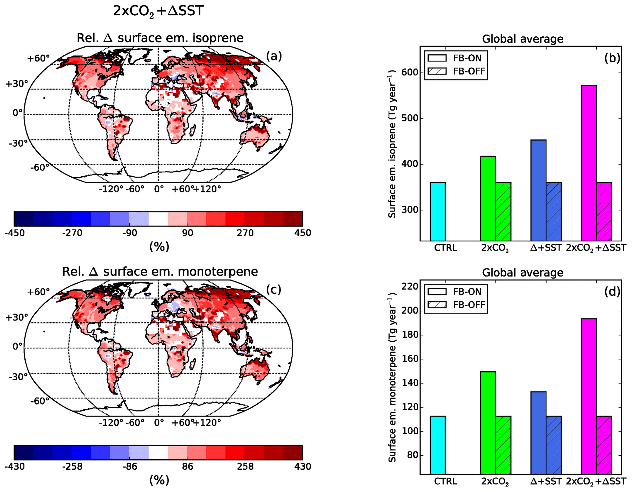
Figure 3 The relative difference between the FB-ON and FB-OFF simulations of the annual average surface emissions of isoprene (a) and monoterpenes (c) for the 2×CO₂ +ΔSST experiment. The relative difference is defined as the (FB-ON − FB-OFF) ∕ FB-OFF. In the bar plots, the yearly global surface emissions of isoprene (b) and monoterpenes (d) for the CTRL simulation as well as the three experiments (both FB-ON and FB-OFF simulations) are shown.

3 Results and discussions

3.1 BVOC emissions and SOA

We will start by discussing the part of the BVOC feedback common to the two branches and then discuss each branch of the feedback separately.

3.1.1 BVOC emissions

The BVOC emissions calculated by NorESM are in line with previous studies. In the CTRL run, the BVOC emissions are 366 Tg yr⁻¹ for isoprene and 115 Tg yr⁻¹ for monoterpenes. These values are in the range of those in Guenther et al. (2012) for monoterpenes but on the lower end for isoprene. For the 2×CO₂ +ΔSST FB-ON simulation, the emissions are 586 Tg yr⁻¹ (+60 %) for isoprene and 198 Tg yr⁻¹ (+73 %) for monoterpenes. The emissions are somewhat lower than estimated for the future climate in previous studies (Laothawornkitkul et al., 2009) but the relative increases are on the high end (Carslaw et al., 2010). The isoprene emissions increase more when the temperature is increased (+ΔSST) than when the CO₂ is doubled, but the opposite is true for monoterpenes; see Fig. 3c and d.

The emissions of isoprene and monoterpenes are higher almost everywhere in the FB-ON simulations with 2×CO₂, +ΔSST and 2×CO₂ +ΔSST than in the FB-OFF simulations with the same setup (see Figs. 3 and S2), in line with the BVOC feedback. The absolute increase in the emissions is largest over the tropical forests, while the relative increase in emissions is greatest over the boreal forests in the Northern Hemisphere (NH). Generally, the CO₂ inhibition of isoprene is masked by the CO₂ and temperature boosts of the vegetation, which leads to a higher leaf area index (LAI) and GPP. In the experiment with only increased CO₂, there are a few areas in Africa and India that seem to have lower isoprene emissions due to CO₂ inhibition. This can be seen as lower isoprene emissions and higher monoterpene emissions in the same place (Fig. S2a and c). This does not occur in the experiments where also the SSTs are increased. Over some regions in the tropics (parts of Africa and the Amazon), especially in the +ΔSST experiment, both monoterpene and isoprene emissions decrease. This is caused by a decrease in the LAI associated with plant mortality that seems to occur because of heat stress. The decrease in LAI leads to a lower albedo in these forest regions, which further increases the temperature, causing more heat stress and creating a feedback mechanism on the vegetation. Nevertheless, the vegetation has had time to adapt to the new temperatures and stabilise by the end of the 30-year spin-up period. The decreases in LAI are smaller in the 2×CO₂ +ΔSST experiments as the vegetation is seeded by CO₂ (Fig. 3a).

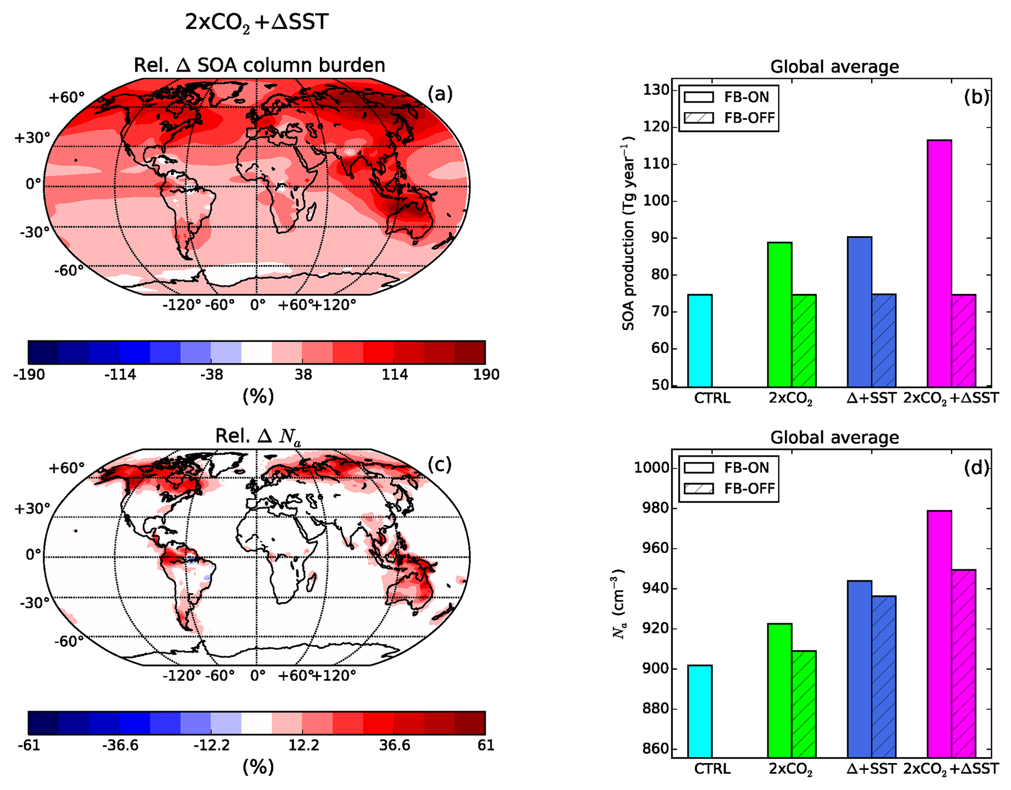
Figure 4 The relative difference between the FB-ON and FB-OFF simulations in the annual average column burden SOA (a) and N_a in the boundary layer (c) for the 2×CO₂ +ΔSST experiment. In the bar plots, the average yearly global production of SOA (b) and the global average N_a in the boundary layer (d) are shown for the CTRL simulation as well as the three experiments (both FB-ON and FB-OFF simulations).

3.1.2 SOA

The higher BVOC emissions in the FB-ON simulations lead to larger SOA production (see Fig. 4b), as expected from the BVOC feedback. The SOA production in the CTRL simulation is 75 Tg yr⁻¹, which is in the range previously estimated by global models (Tsigaridis et al., 2014; Glasius and Goldstein, 2016). The SOA production in the FB-ON simulations is similar for the 2×CO₂ and +ΔSST experiments (90 and 92 Tg yr⁻¹) while the combined effect of higher CO₂ and temperature gives a higher SOA production, with values of 115 Tg yr⁻¹. The column burden of SOA is higher over the entire globe when the BVOC feedback is on compared to when it is turned off, except in the +ΔSST experiment over and downwind of the regions where the BVOC emissions decrease; see Figs. 4a and S3b. The largest absolute increase of column burden SOA is over the tropical forests, while the largest relative increases are over the Arctic and sub-Arctic. The fraction of SOA in the aerosol particles is also higher when the feedback is turned on, which leads to a reduction in the hygroscopicity of the particles (not shown).

3.1.3 Aerosol number and size

Not only is the mass of the aerosol particles affected by higher levels of BVOCs but also the number concentration of aerosol particles and their sizes. The changes in the number concentration and size of the particles vary with region. The largest difference in N_a between the FB-ON and FB-OFF simulations occurs over, and downwind of, the tropical rain forests, as well as over the boreal forests in the NH (see Fig. 4c). The relative difference is largest over the boreal forests in the NH where the particle number concentrations are generally low. The largest absolute differences on the other hand occur in the tropics. Over regions where the emissions decrease (in the +ΔSST experiment), the N_a decreases (Fig. S3d).

Figure 5 Annually averaged aerosol number size distributions in the boundary layer for the boreal forest region (lat.: 55 to 70^∘ N, long.: 180^∘ W to 180^∘ E) and the region around the tropical islands in southeast Asia (lat.: 20^∘ S to 20^∘ N, long.: 90–130^∘ E). In panels (a) and (c), the distributions from the CTRL and the three experiments are plotted, while in panels (b) and (d), the differences between the FB-ON and FB-OFF simulations are plotted.

In order to investigate the effect on the sizes of the particles, we analysed the averaged boundary layer aerosol size distributions for two of the regions most affected by the feedback: the boreal forests and the tropical islands in southeast Asia. The size distributions are created from the number median radius and standard deviations of the 12 particle mixtures in OsloAero (Kirkevåg et al., 2018). Over the boreal forests, the higher BVOC emissions result in more particles in the Aitken mode (Fig. 5a and b). The enhanced growth of the particles also results in more particles in the accumulation mode and in a shift to larger sizes of the Aitken mode, which results in a small decrease in the number of particles below 25 nm. In the tropics, there is a larger (smaller) absolute (relative) increase in Aitken-mode particles. The shift in the size distribution due to more condensing vapours is larger here than over the boreal forests and results in decreasing particle concentrations up to 70 nm. The biggest changes in both number and shift in size distribution are seen in the 2×CO₂ +ΔSST experiment. The changes in particle sizes occur further downwind from the sources than the changes in aerosol number concentrations which are more restricted to areas close to the sources, in particular in the tropics.

3.2 The T-feedback branch

3.2.1 CCN

The CCN response of the feedback is a combination of the changes in N_a, particle sizes and hygroscopicity. The CCN concentrations are generally higher when the feedback is turned on, as is expected from the feedback (Fig. 1). However, at low supersaturations (0.2 %), the CCN concentration over some regions (in particular over the boreal forests), is lower in the simulations with the feedback turned on (Fig. 6a). The cause for this is the large amount of Aitken-mode particles formed through new particle formation. The smaller particles compete with the larger particles for the water vapour, which reduces the number of aerosol particles that can activate into cloud droplets at low supersaturations. The concentrations of CCN in these regions are very low and the absolute decrease in CCN is small. Moreover, it should be noted that the CCN concentration in the model is calculated only for the cloud-free areas in the grid boxes. Thus, the particles that are activated into cloud droplets are not included in the CCN concentrations. At higher supersaturations (1 %), also particles at smaller sizes can be activated, and thus the feedback results in more CCN almost everywhere (Fig. 6c). The areas downwind of the tropics, where the feedback mainly results in an increase in particle size, have higher CCN at both levels of supersaturation. The effect of increasing particle sizes and number generally dominates the effect of decreased particle hygroscopicity since the feedback contributes with increasing number of CCN.

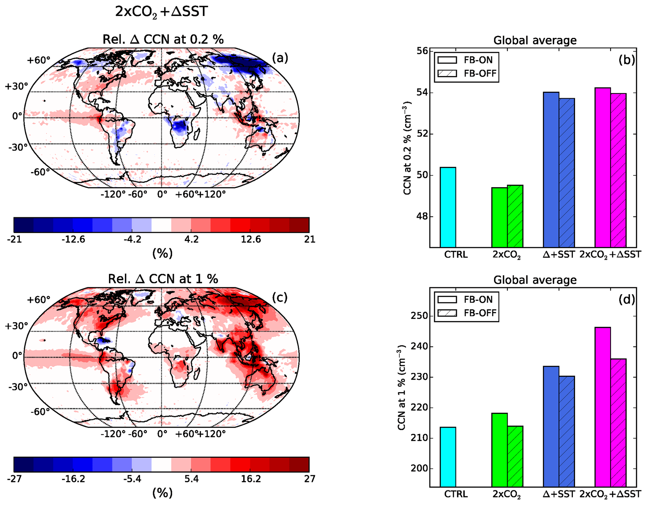
Figure 6 The relative difference between the FB-ON and FB-OFF simulations in the annual average CCN at 0.2 % (a) and 1 % (c) in the boundary layer, for the 2×CO₂ +ΔSST experiment. In the bar plots, the globally averaged CCN at 0.2 % (b) and 1 % (d) in the boundary layer are shown for the CTRL simulation as well as the three experiments (both FB-ON and FB-OFF simulations).

3.2.2 Cloud properties

The effect from the BVOC feedback on the clouds is mainly seen over and downwind of the regions where the BVOC emissions change the most. The vertically averaged CDNC generally increase (as is expected from the BVOC feedback), mainly north of 45^∘ N and in the tropics Fig. 7a. The weakest response of the CDNC to the feedback occurs in the experiment where only CO₂ has been changed (Figs. 7b and S5). In the experiment with only increased SST, the CDNC is higher mainly in the Northern Hemisphere since the BVOC emissions in parts of the tropics decrease (Fig. S5b). The higher levels of CDNC occur predominantly during the local summer when the BVOC emissions are the highest.

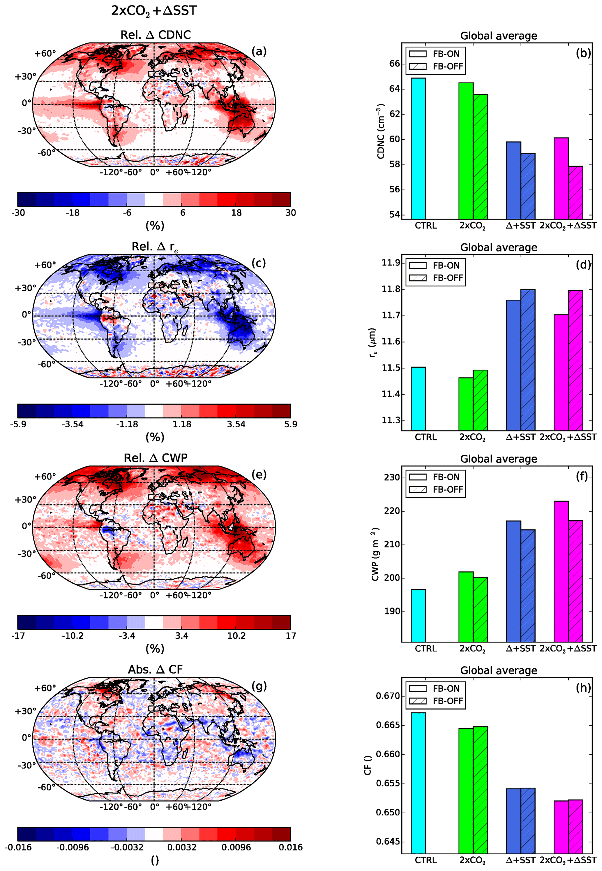
Figure 7 The relative/absolute difference between the FB-ON and FB-OFF simulations in the annual vertically averaged CDNC (a), the vertically averaged r_e (c), the CWP (e) and the total CF (g) for the 2×CO₂ +ΔSST experiment. In the bar plots (b, d, f, h), the globally averaged values of the same variables are shown for the CTRL simulation as well as the three experiments (both FB-ON and FB-OFF simulations). For the CDNC, r_e and CWP, the in-cloud values are used.

The increasing CDNC associated with the feedback is accompanied by a decrease in cloud droplet effective radius (r_e) and an increasing cloud water path (CWP) (Fig. 7c and e). The total cloud fraction (CF) does however not seem to be impacted to the same extent (see Fig. 7g and h), which may be an effect of the nudging. There is an increase in the CF over the boreal forests, mainly during winter, by up to 4 %. In summer, there is an increase in low- and mid-level clouds over the Arctic and NH midlatitudes. This is accompanied by a decrease in the high-level clouds and therefore does not show up clearly in Fig. 7g. In the tropics, there are no systematic changes in the cloud fraction as a result of the feedback.

The strongest and most widespread difference in the cloud microphysical effects occurs in the NH midlatitudes and high latitudes. One cause for this is the cloud cover and cloud types present close to the emission regions. The clouds in the midlatitudes and high latitudes are commonly stratiform, for which the model includes N_a in the calculations of CDNC (through the Abdul-Razzak and Ghan, 2000 scheme for activation). The differences in CDNC are not as widespread in the tropics, since shallow and deep convection (which aerosols generally do not affect in ESMs) are the dominant cloud types here. Another cause for the more widespread cloud changes in the NH is the larger land areas here, i.e. larger areas where the emissions differ.

3.2.3 Cloud forcing

The potential of the BVOC feedback to affect future climate will now be evaluated by investigating the changes in cloud forcing between the FB-ON and FB-OFF simulations. Since we cannot determine the full temperature response of the feedback, the differences in forcing between the FB-ON and FB-OFF simulations will be used to estimate the potential climate impact of the changed cloud properties. The patterns of the difference in the cloud forcing between the simulations with the FB turned on and the FB turned off (Fig. 8a and c) resemble the patterns of the difference in CDNC (Fig. 7a). The higher CDNC in the high latitudes and midlatitudes associated with the FB is accompanied by a decrease in the NCF_Ghan by up to −11 W m⁻² during the 3 summer months; see Fig. 8a. The effect of the feedback is seen mainly during the local summer when the BVOC emissions are the highest. The differences in NCF_Ghan are smallest in the 2×CO₂ experiment and strongest in the 2×CO₂ +ΔSST experiment (Figs. 8 and S6).

Figure 8 The absolute difference between the FB-ON and FB-OFF simulations for the NCF_Ghan during June, July and August (a), December January and February (c), as well as the NCF_S during December, January and February (e) for the 2×CO₂ +ΔSST experiment. In the bar plots (b, d, f), the globally averaged values of the same variables are shown for the CTRL simulation as well as the three experiments (both FB-ON and FB-OFF simulations).

The feedback does not only contribute with an enhanced negative cloud forcing though. The difference in NCF at the surface (Δ NCF_S) between the FB-ON and FB-OFF simulations is positive over the NH boreal forests during winter in the experiments with increased SST (Figs. 8e and S6f). The changes in microphysical properties as well as cloud cover lead to an increase in the positive long-wave cloud forcing (LWCF) at the surface, which is larger than the corresponding increase in negative short-wave cloud forcing (SWCF). It can be concluded that the BVOC feedback can contribute to both enhanced and reduced negative cloud forcing depending on region and season. Nevertheless, the difference in yearly global average NCF_Ghan is −0.43 W m⁻² (SWCF_Ghan −0.45 W m⁻², LWCF_Ghan 0.02 W m⁻²) between the FB-ON and FB-OFF simulations in the 2×CO₂ +ΔSST experiment, indicating that the feedback can contribute with a potentially important impact on the future climate on a global scale.

The strongest and most widespread negative cloud forcing associated with the feedback is seen in the Arctic during summer. This is interesting since the Arctic is currently, and is expected to continue, experiencing the largest warming in response to the increasing atmospheric concentrations of greenhouse gases (IPCC, 2013). The strong impact of the BVOC feedback in the Arctic during summer could possibly counteract part of this Arctic amplification. The large impact of the feedback in the NH midlatitudes and high latitudes also results in a quite large difference in the effect of the feedback between the hemispheres. The difference in the NCF_Ghan, between the FB-ON and FB-OFF simulations for the 2×CO₂ +ΔSST experiments, is −0.56 W m⁻² in the NH, while in the SH it is −0.30 W m⁻².

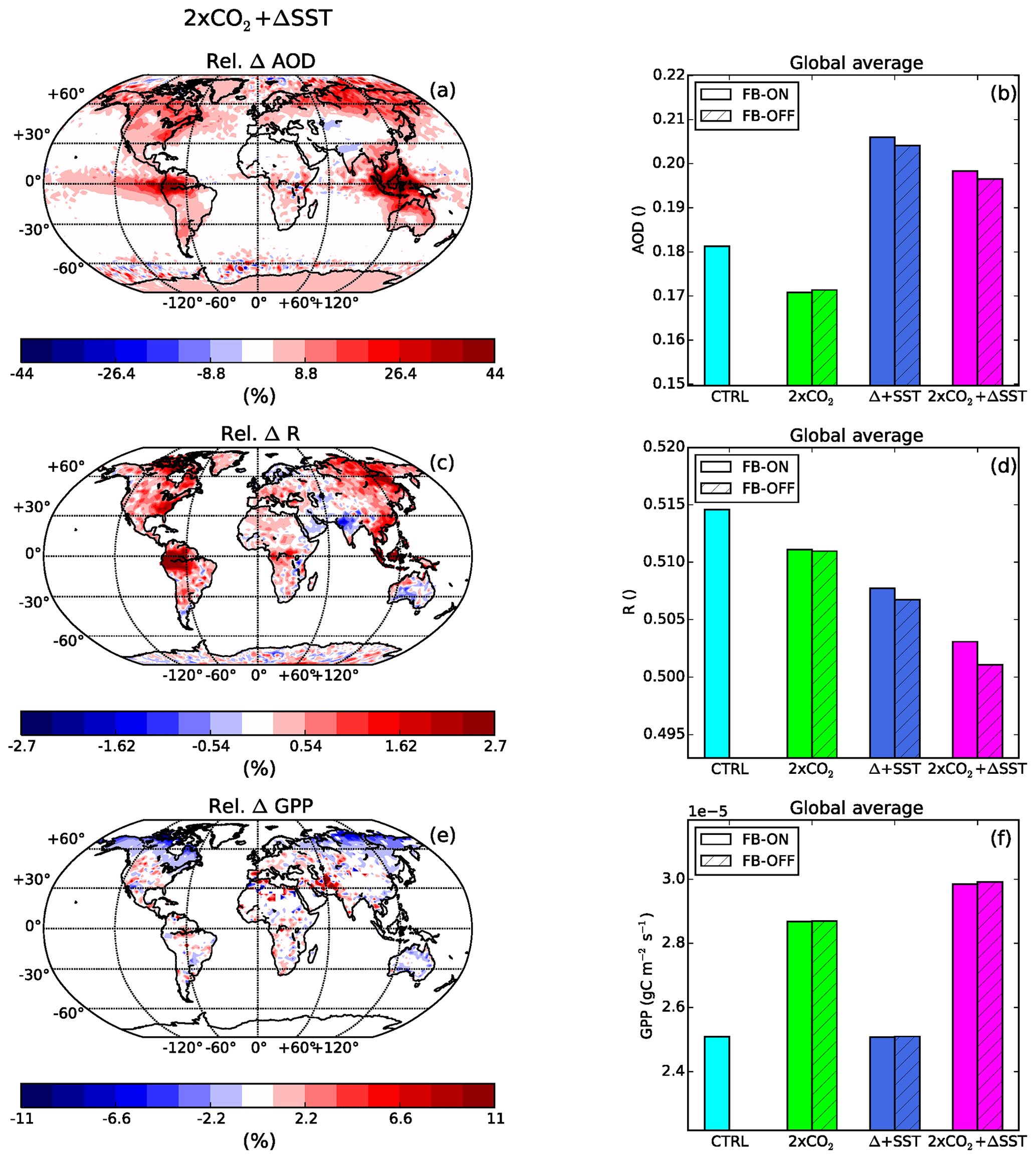
Figure 9 The relative difference between the FB-ON and FB-OFF simulations in the annually average AOD (a), R (c) and GPP (e) for the 2×CO₂ +ΔSST experiment. In the bar plots (b, d, f), the globally averaged values of the same variables are shown for the CTRL simulation as well as the three experiments (both FB-ON and FB-OFF simulations).

3.3 The GPP-feedback branch

3.3.1 AOD

The higher aerosol loading associated with the feedback also results in higher values for the aerosol optical depth (AOD), in line with the feedback in Fig. 1. The largest relative differences between the FB-ON and FB-OFF simulations occur over, and downwind of, the tropical forest and the boreal forests in the NH; see Fig. 9a. The AOD effects are largest in the local summer when the emissions are the highest.

3.3.2 Diffuse radiation

The ratio between the diffuse radiation and the global radiation is, according the BVOC-feedback hypotheses, expected to increase with higher aerosol scattering. Our model simulations show only a small relative difference in R (maximum 5 %) between the FB-ON and FB-OFF simulations (Fig. 9c). The regions where there is a strong difference in R between the FB-ON and FB-OFF simulations correspond to the regions with the largest change in AOD. However, a statistical analysis of the differences between the monthly means from the FB-ON and FB-OFF simulations shows that the correlation coefficient between the difference in R and the difference in total cloud cover (0.53) is higher than between the difference in R and the difference in AOD (0.08); see Fig. 10a and b. Small changes in the cloud cover can offset the AOD effects on R. Changes in cloud cover can therefore explain the decreases in R over, e.g. Scandinavia (Fig. 9), even though the AOD increases there. The increase in R is expected from the BVOC feedback but the larger dependency in R on cloud fraction than AOD was not expected.

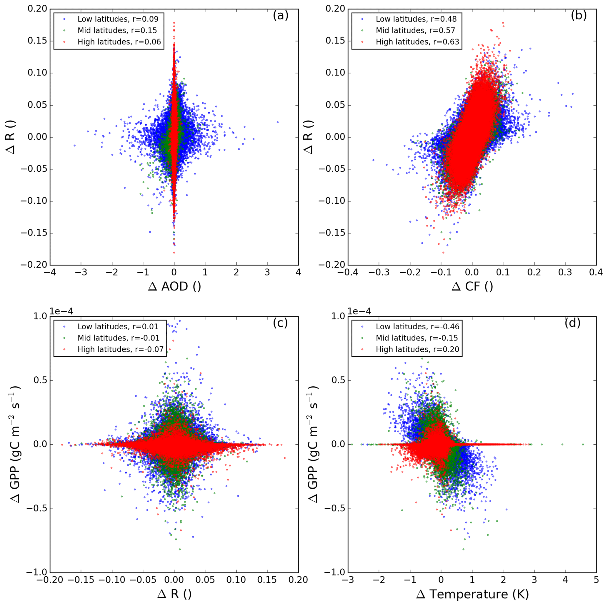
Figure 10 Scatter plots of the absolute differences (FB-ON − FB-OFF) in AOD and R in panel (a), CF and R in panel (b), GPP and R in panel (c) and GPP and temperature in the lowest model layer in panel (d). Data from all three experiments (2×CO₂,  +ΔSST and 2×CO₂ +ΔSST) are included. Each dot is a monthly average for one grid box. Only grid boxes with a land fraction of 1 and GPP greater than zero are included. The dots are coloured according to latitude bands (high latitudes: 90–55^∘ S and 55–90^∘ N, midlatitudes: 55–30^∘ S and 30–55^∘ N, low latitudes: 30^∘ S–30^∘ N) and the correlations coefficient r for each region is shown in the legend. Based on the model output, AOD does not drive diffuse radiation fraction, but cloud fraction does; and diffuse radiation does not drive gross primary product, but temperature does.

3.3.3 GPP

Next, we will investigate the relationship between R and GPP. Neither in the maps nor in the statistical analyses do we find any strong relationship between R and GPP; see Figs. 9e and 10c. The positive effect of diffuse radiation on vegetation growth is included in CLM (Oleson et al., 2013) but it seems like other factors perturbed by the T branch are affecting the vegetation more. Moreover, the difference in R between the FB-ON and FB-OFF simulations was quite small. The relationship between R and GPP is also affected by changes in the total amount of radiation. If the total radiation decreases sufficiently, an increase in R will not boost GPP (Knohl and Baldocchi, 2008). There is a negative correlation between the change in R and the change in the total visible radiation in our experiments, and the total visible radiation is generally lower in the feedback on simulations (see Fig. S8a). The hypothesised boost of GPP by R might therefore be masked by the change in the total visible radiation. Since the focus of this study is the effect of the feedback on a global scale, we have chosen not to look into if we can find the effect of R on GPP in certain conditions or locations.

The GPP instead seems to respond to changes associated with the T-feedback branch (Fig. 10d). In particular, there is a decrease of GPP in the sub-Arctic during the summer months associated with lower temperatures caused by the enhanced negative NCF_Ghan. Even though we are running with fixed SSTs, the temperatures over land can change somewhat in response to the changed forcing. In addition, a decrease in total visible radiation reaching the vegetation, associated with the increase in low-cloud cover in this region, can contribute to the decrease in GPP. Overall, the GPP is slightly lower in the simulations where we include the feedback, which is opposite to what is expected from the feedback in Fig. 1. These results are in contrast to the results by Rap et al. (2018), which did not include the effects from the T branch in their study. In our study, it seems that the effects from the T branch of the BVOC-feedback loop is dominating over the GPP branch. The GPP branch may however be important on local scales ot resolvable by NorESM.

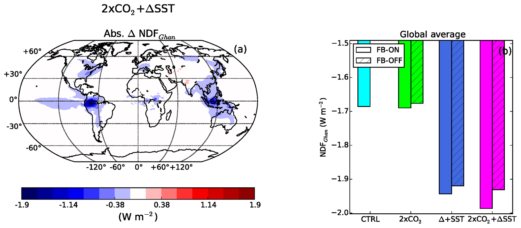
Figure 11 The absolute difference between the FB-ON and FB-OFF simulations in the annual average NDF_Ghan (a) for the 2×CO₂ +ΔSST experiment. In panel (b), the globally averaged NDF_Ghan for the CTRL simulation as well as the three experiments (both FB-ON and FB-OFF simulations) are shown.

3.4 Direct aerosol forcing

The scattering of radiation from aerosols in the atmosphere did not seem to impact the GPP significantly in our experiments, but we do find a direct impact on climate. The annual average NDF_Ghan is locally down to −2.2 W m⁻² when the feedback is turned on; see Fig. 11a. The largest differences in NDF_Ghan between the FB-ON and FB-OFF simulations is seen close to the sources and over the regions that have large absolute changes in the emissions, i.e. the tropics. Globally averaged, the difference in NDF_Ghan is −0.06 W m⁻² for the 2×CO₂ +ΔSST experiment. This is approximately 15 % of the difference in forcing from the clouds. The magnitude of the differences in the NDF_Ghan indicates that the BVOC feedback can provide an, at least regionally, enhanced negative forcing also through the direct aerosol forcing.

3.5 Future lower aerosol loading

In order to investigate how the impact of the feedback changes if the aerosol emissions decrease in the future, we also ran the 2×CO₂ +ΔSST experiment with lower anthropogenic aerosol emissions. The BVOC emissions in 2×CO₂ +ΔSST LA FB-ON simulation are almost the same as those in the 2×CO₂ +ΔSST FB-ON simulation (4 % and 3 % higher for isoprene and monoterpenes). The response to the feedback is however larger in the experiment with lower anthropogenic emissions. The relative differences in N_a are larger, especially over regions with large anthropogenic emissions in PD. This indicates that BVOCs will be more important for aerosol formation in the future, if the anthropogenic emissions decrease. The relative CDNC difference is also greater in the experiment with low anthropogenic emissions in both the tropics and the NH. There are areas (such as southeast Asia) where the relative differences in CDNC are close to zero in the 2×CO₂ +ΔSST experiment and up to 30 % in the 2×CO₂ +ΔSST LA experiment. That the effects on the clouds are largest in the 2×CO₂ +ΔSST LA experiment is not surprising, since clouds formed in clean condition are most susceptible to aerosol perturbations (Spracklen and Rap, 2013).

Table 2 Difference in the global annual average NCF_Ghan, NDF_Ghan and total aerosol forcing (TAF_Ghan) between the FB-ON and FB-OFF simulations.

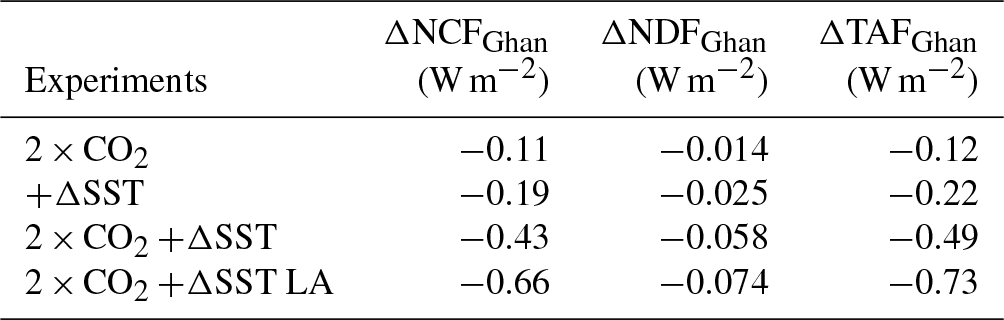
The stronger BVOC impact on the clouds in the experiment with lower aerosol loading result in a larger impact from the feedback on the radiation budget. The difference in the yearly global average NCF_Ghan for the 2×CO₂ +ΔSST LA is 53 % higher than for the 2×CO₂ +ΔSST experiment; see Table 2. In addition, the direct effect associated with the feedback is larger when the anthropogenic aerosol load is reduced. The difference in NDF_Ghan is 29 % higher for the experiment with lower aerosol loading. These results show that the importance of the BVOC feedback will become substantially greater if, as expected, the anthropogenic aerosol emissions are reduced in the future. These results are interesting, especially since some large emitters have already started reducing their SO₂ emissions (Li et al., 2017). The total aerosol forcing associated with the feedback in the 2×CO₂ +ΔSST (LA) experiment is −0.49 (−0.73) W m⁻², which is 13 (20) % of the positive radiative forcing (calculated according to Myhre et al., 1998) associated with a similar doubling of CO₂.

3.6 Limitations and uncertainties

The investigation of the effects of BVOCs is challenging since it involves complex interactions not only in the atmosphere but also in the biosphere. In this investigation, the focus has been on the potential atmospheric consequences of increased BVOC emissions. However, the future BVOC emissions are highly sensitive to what will happen to the vegetation. This was clearly seen in our simulations where we increased only the SST and found that GPP is reduced in several regions due to heat stress. This cancels or even reverses the BVOC feedback in these regions. How future vegetation will respond to climate change is still highly uncertain (Friend et al., 2014).

Our simulations do not allow changes in the distribution of the vegetation and therefore do not include any effects of geographical shifts in vegetation. A poleward shift in the vegetation could increase the BVOC emissions in these regions (Peñuelas and Staudt, 2010). Nevertheless, changes in surface albedo, as well as latent and sensible heat fluxes associated with such shifts (Bonan, 2008), could counteract/dominate parts of the effects seen from the increased BVOC emissions. Changes in land use also have the potential to affect the BVOC emissions but have not been taken into account in this study. A recent study by Hantson et al. (2017) including land use found no increase in BVOC emissions at the end of the century. However, they also note that the land use scenarios are highly uncertain.

There are also uncertainties associated with the emissions from the plants themselves. In MEGAN2.1, used in this study, CO₂ inhibition is included for isoprene. There are indications that the inhibition also affects monoterpenes and some studies include it also for monoterpenes (Arneth et al., 2016). Including CO₂ inhibition for monoterpenes could have reduced the difference in monoterpene emissions between the FB-ON and FB-OFF simulations and reduced the effect of the feedback. Plant stress due to heat or insect infestations can affect the magnitude and type of BVOC emissions (Zhao et al., 2017). These effects are very complex and have not been included in this study.

During the setup of the experiments of this study, we found that the model was sensitive to the diurnal variation in the BVOC emissions (also described in Sect. 2.2). The column burden of isoprene (monoterpene) was, on a global average, 57 (13) % higher when monthly averaged emission files without diurnal variation were used in the model instead of the interactive emissions. Adding a diurnal variation (the one included in CAM5.3) to the monthly emissions field improves the column burden values for isoprene, but for monoterpenes, the column burdens stay high. The resulting difference in the column burden of SOA (+5 % on a global average) is dampened by complex processes associated with nucleation and condensation. However, the lack of autocorrelation between the emissions and oxidants (when using monthly emissions) can result in longer lifetimes for the BVOC and a shift in region and level where the SOA formation occurs. This has been shown to affect the indirect aerosol effect (Karset et al., 2018). Monthly BVOC emission files should therefore be used with caution. In this study, prescribed oxidant fields at PD conditions with applied diurnal variation for OH and HO₂ were used. Running the model with more advanced gas-phase chemistry would have simulated the interactions between the BVOCs and the oxidants more realistically.

New particle formation, BVOC and SOA parameterisations are now implemented in many ESMs but are still under development and associated with uncertainties (e.g. Tsigaridis and Kanakidou, 2018; Makkonen et al., 2014; Gordon et al., 2016). The BVOC feedback mechanism is highly sensitive to the parameterisations associated with new particle and SOA formation. The yields associated with the formation of LVSOA and SVSOA from monoterpenes and isoprene are largely uncertain, which may significantly affect the feedback. The parameterisations of nucleation rates and early growth of the particles can also have a strong impact on the simulations of the feedback. Moreover, the SOA scheme in NorESM does not account for effects of temperature on partitioning of SOA precursors. Warmer temperatures might lead to less SOA formation with same amount of precursors, which would reduce the feedback. In addition, the SOA formation from biogenic precursors could be highly susceptible to modification by anthropogenic emissions of VOCs (Spracklen et al., 2011), which are not currently included in NorESM. We hope that the importance of the feedback found in this study will inspire further development of these parameterisations in ESMs.

Running the model with fixed SSTs and nudging provides a nice setup to study each step in the feedback loops at low computational cost, but it also comes with some limitations. The nudging enabled us to run the FB-ON and FB-OFF simulations with the same meteorological conditions. We can therefore conclude that the difference between the simulations was only associated with the BVOC emissions and the feedback and not caused by natural variability. The nudging does however mean that any impacts of the feedback on horizontal winds and pressure are not captured in this investigation. Moreover, the fixed SSTs and sea ice limit the temperature response to the feedback. There is some temperature response to forcing induced by the feedback over land but not over the oceans. The second-order feedbacks, such as decreasing BVOC emissions associated with the temperature decrease due to the enhanced negative cloud and direct forcing, will not be properly simulated with this setup. Investigating the feedback with free-running simulations using a coupled version of NorESM would be a very nice complement to this study.

In this paper, we have focused on the BVOC feedback mechanisms shown in Fig. 1, but there are other indirect effects of BVOCs that could influence the feedback that are not included in this study. Two such effects involve impacts on ozone production and methane lifetime. When BVOCs are oxidised in the atmosphere, they affect the chemical composition as well as the oxidising capacity of the atmosphere. Firstly, BVOCs can contribute to enhanced ozone production if sufficient NO_x is available, while they can give a net consumption in low NO_x conditions (Monks et al., 2015). Secondly, the oxidation of BVOCs can decrease the oxidation capacity of the atmosphere, thus increasing the atmospheric lifetime of methane. Both of these effects could result in a positive radiative forcing with increased BVOC emissions. Previous studies have found BVOC-induced changes in the direct aerosol forcing to be roughly balanced by the changes in the forcing from ozone and methane (Unger, 2014; Scott et al., 2018b). This indicates that part of the forcing (the NDF in this study is 12 % of the total forcing) associated with BVOC feedback investigated in this paper could be offset by changes in ozone and methane lifetime.

Moreover, some of the processes in the BVOC feedback investigated here may affect the carbon budget; however, such effects are out of the scope of this paper.

4 Conclusions

An ESM has been used to investigate two feedbacks induced by increased emissions of BVOCs in response to higher CO₂ concentrations and/or temperature (Fig. 1). We find that higher BVOC emissions indeed lead to the formation of more SOA mass, as well as both higher aerosol number concentrations and larger particle sizes. This leads to clouds with more and smaller droplets and higher cloud water path. The changes in the clouds are found to contribute with an enhanced negative cloud forcing, confirming the possibility for BVOCs to contribute with a negative climate feedback. The feedback is strongest over and downwind of the boreal and tropical forests. Solely increasing the CO₂ levels produces a somewhat weaker feedback response than solely increasing the temperatures, but the strongest response comes from increasing both CO₂ and temperature.

In this investigation, we do not find that the enhanced aerosol scattering leads to a boost of GPP globally (see Fig. 1). The response of the GPP is instead dominated by the BVOC-induced changes of the clouds. The enhanced aerosol scattering associated with the feedback is however found to lead to a stronger negative forcing (direct effect). We would therefore suggest modifying the BVOC feedback in Fig. 1 as can be seen in Fig. 12. Because the GPP seems to be more affected by the cloud changes than the AOD changes, the arrows between AOD and GPP have been dashed. However, AOD can now be seen having a negative feedback on temperature. The combined effects from both altered cloud properties and AOD are found to contribute with a negative radiative effect of −0.49 W m⁻². To put this number in context, the radiative forcing from a doubling of CO₂ is about 3.7 W m⁻². Thus, the forcing associated with the BVOC feedback could offset this by about 13 %, or even up to 20 %, given a strong reduction in anthropogenic aerosols. This leads us to conclude that the BVOC feedback is very relevant for estimating climate sensitivity with ESMs and providing model-based projections of the future climate.

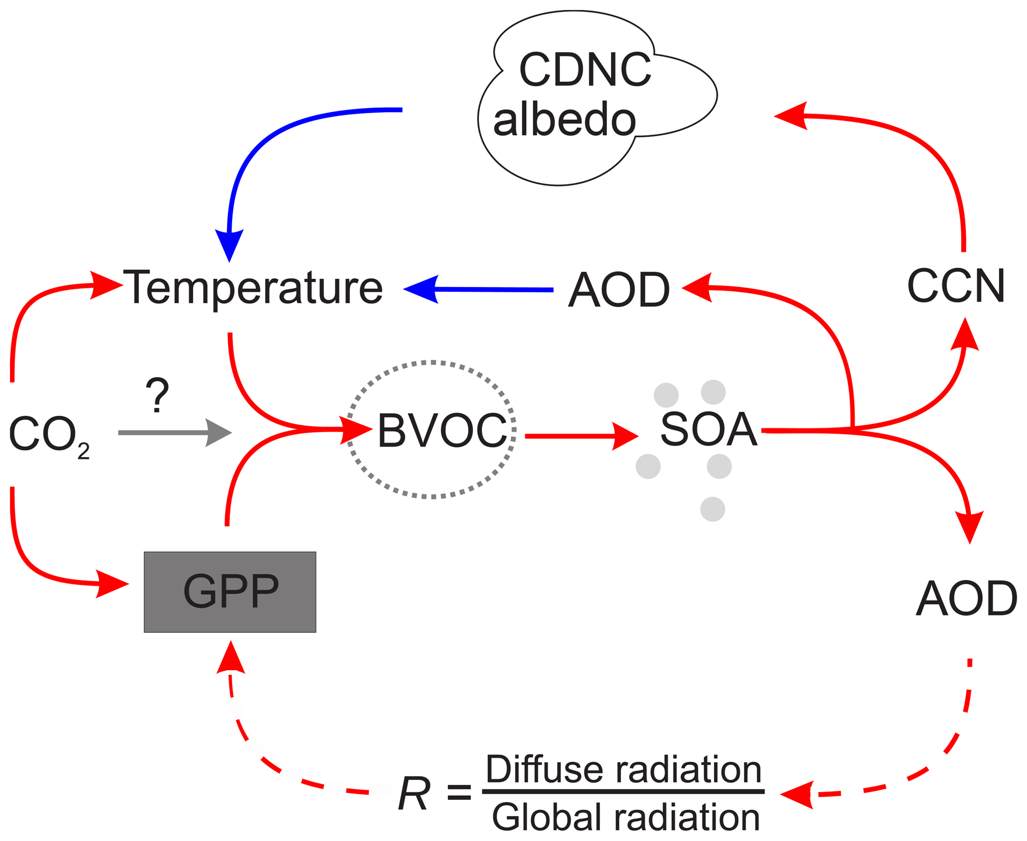
Figure 12 Our modified version of the BVOC feedback according to the results from this study. The red arrows in the figure indicate that if the variable at the start of the arrow increases, then the variable at the end of the arrow is also expected to increase. A blue arrow on the other hand means that an increase in the variable at the start of the arrow is expected to result in a decrease in the variable at the end of the arrow. The GPP branch of the feedback now has dashed lines and the changed AOD has been found to impact temperature.

There are still large uncertainties associated with the processes associated with the BVOC feedback, both in models and measurements. The aim of this study was not to provide a final answer regarding the importance of the feedback. Instead, we wanted to use the current knowledge implemented in NorESM to test the potential importance of including these processes in an ESM when predicting the future climate. The results from this study should encourage and inspire further research to improve the representation of these processes in ESMs.