the Creative Commons Attribution 4.0 License.
the Creative Commons Attribution 4.0 License.
 | 28 Feb 2019
Satellite-derived emissions of carbon monoxide, ammonia, and nitrogen dioxide from the 2016 Horse River wildfire in the Fort McMurray area
Cristen Adams
Chris A. McLinden
Mark W. Shephard
Nolan Dickson
Enrico Dammers
Jack Chen
Paul Makar
Karen E. Cady-Pereira
Naomi Tam
Shailesh K. Kharol
Lok N. Lamsal
Nickolay A. Krotkov
In May 2016, the Horse River wildfire led to the evacuation of ∼ 88 000 people from Fort McMurray and surrounding areas and consumed ∼ 590 000 ha of land in Northern Alberta and Saskatchewan. Within the plume, satellite instruments measured elevated values of CO, NH3, and NO2. CO was measured by two Infrared Atmospheric Sounding Interferometers (IASI-A and IASI-B), NH3 by IASI-A, IASI-B, and the Cross-track Infrared Sounder (CrIS), and NO2 by the Ozone Monitoring Instrument (OMI). Daily emission rates were calculated from the satellite measurements using fire hotspot information from the Moderate Resolution Imaging Spectroradiometer (MODIS) and wind information from the European Centre for Medium-Range Weather Forecasts (ECMWF) ERA5 reanalysis, combined with assumptions on lifetimes and the altitude range of the plume. Sensitivity tests were performed and it was found that uncertainties of emission estimates are more sensitive to the plume shape for CO and to the lifetime for NH3 and NOx. The satellite-derived emission rates were ∼ 50–300 kt d−1 for CO, ∼ 1–7 kt d−1 for NH3, and ∼ 0.5–2 kt d−1 for NOx (expressed as NO) during the most active fire periods. The daily satellite-derived emission estimates were found to correlate fairly well (R∼0.4–0.7) with daily output from the ECMWF Global Fire Assimilation System (GFAS) and the Environment and Climate Change Canada (ECCC) FireWork models, with agreement within a factor of 2 for most comparisons. Emission ratios of NH3∕CO, NOx∕CO, and NOx∕NH3 were calculated and compared against enhancement ratios of surface concentrations measured at permanent surface air monitoring stations and by the Alberta Environment and Parks Mobile Air Monitoring Laboratory (MAML). For NH3∕CO, the satellite emission ratios of ∼ 0.02 are within a factor of 2 of the model emission ratios and surface enhancement ratios. For NOx∕CO satellite-measured emission ratios of ∼0.01 are lower than the modelled emission ratios of 0.033 for GFAS and 0.014 for FireWork, but are larger than the surface enhancement ratios of ∼0.003, which may have been affected by the short lifetime of NOx. Total emissions from the Horse River fire for May 2016 were calculated and compared against total annual anthropogenic emissions for the province of Alberta in 2016 from the ECCC Air Pollutant Emissions Inventory (APEI). Satellite-measured emissions of CO are ∼1500 kt for the Horse River fire and exceed the total annual Alberta anthropogenic CO emissions of 992.6 kt for 2016. The satellite-measured emissions during the Horse River fire of ∼30 kt of NH3 and ∼7 kt of NOx (expressed as NO) are approximately 20 % and 1 % of the magnitude of total annual Alberta anthropogenic emissions, respectively.
- Article
(5279 KB) - Full-text XML
-
Supplement
(76 KB) - BibTeX
- EndNote


The 2016 Horse River wildfire (MNP LLP, 2017) was first observed on 1 May 2016 approximately 7 km south-west of Fort McMurray and grew rapidly. On 3 May 2016, the fire entered the urban service area of Fort McMurray, leading to the evacuation of ∼ 88 000 people, damaging multiple structures, and threatening nearby communities, oil sands camps, and facilities. The fire then moved eastward toward Saskatchewan and, after 2 months of firefighting efforts, was determined under control on 4 July 2016. The fire consumed 589 522 ha in Northern Alberta and Saskatchewan and led to an estimated USD 3.58 billion in insured losses (Insurance Bureau of Canada, 2016).
The number and size of wildfires in North America have been increasing over the past few decades due to various factors, such as drought conditions, changes in land use, and fire management practices (Romero-Lankao et al., 2014). In Canada the number of wildfires and total burned area increased between 1961 and 2015 (Landis et al., 2018). In Alberta, the number of wildfires has increased, but the total annual acreage burned has been variable, with several years of anomalously large burn areas (Landis et al., 2018). The annual burn area in the boreal forest is projected to increase, with some of the largest increases predicted in north-eastern Alberta (Boulanger et al., 2014), which could affect ecosystems (e.g., Stralberg et al., 2018), air quality (e.g., Yue et al., 2015), and the climate (e.g., Oris et al., 2014).
Emissions from forest fires have a large effect on global and regional air quality; more than 10 % of global CO from wildfires is emitted over middle and high latitudes (Langmann et al., 2009). Emission factors characterise the amount of a gas released per kg of fuel consumed (g kg−1) and are often used in air quality models to estimate emissions from wildfires. Emission factors for a given land cover type vary naturally depending on burning conditions (flaming versus smouldering phases) and fuel type (stems, leaves, or needles). The flaming versus smouldering phases of combustion also have different emission factors for the same species. For example, NOx and CO2 are emitted in larger quantities during flaming periods, while NH3 and CO are emitted in larger quantities during smouldering periods (e.g., Andreae and Merlet, 2001). The occurrence of flaming and smouldering phases depends on the moisture content of the fuel (Chen et al., 2010) and can vary diurnally, with more active flaming during the day, as well as spatially between the fire front and areas of residual burning (e.g., Langmann et al., 2009; McRae et al., 2005). Emission factors also vary with fuel type for, e.g., stems, leaves, or needles. A study in north-western Alberta found that deciduous trees (e.g., trembling aspen) contain more nitrogen than conifers (e.g., white spruce) (Jerabkova et al., 2006); this might be expected to lead to larger emissions of NOx and NH3 for trembling aspen. Akagi et al. (2011) estimated variability in boreal forest emission factors from aircraft and laboratory studies of 35 % for CO, 85 % for NH3, and 77 % for NOx.
Due to their spatial and temporal coverage, satellite remote sensing instruments can capture some of this natural variability by estimating emissions and emission factors over various seasons, burning conditions, fuel types, and moisture content. Previous studies using satellite CO, NH3, and NO2 data have assessed the relationship between these species (e.g., Coheur et al., 2009; Krol et al., 2013; Luo et al., 2015; Paulot et al., 2017; Pechony et al., 2013; R'Honi et al., 2013; Whitburn et al., 2015; Yurganov et al., 2011) and have also estimated emissions and emission factors (e.g., Mebust and Cohen, 2014; Mebust et al., 2011; Schreier et al., 2014, 2015; Tanimoto et al., 2015; Whitburn et al., 2015, 2016b). Emission factors have also been estimated using ground-based Fourier transform infrared (FTIR) spectrometers (e.g., Lutsch et al., 2016).
The Horse River fire provides an excellent opportunity to evaluate methods for estimating emissions from satellite. Due to the close proximity of the fire to industry and communities, there is a relatively extensive surface monitoring network in the region, and many surface air quality datasets are collected routinely in the area. These networks captured detailed information about the wildfire plume (Landis et al., 2018; Wentworth et al., 2018), which can be used to support the satellite-based estimates. In this study, we estimate emissions from several satellite instruments: CO measured by the two Infrared Atmospheric Sounding Interferometers (IASI-A and IASI-B), NH3 measured by IASI-A, IASI-B, and the Cross-track Infrared Sounder (CrIS), and NO2 measured by the Ozone Monitoring Instrument (OMI). We compare emission estimates with model data, explore relationships between CO, NH3, and NOx, and derive emission factors from the satellite data.
Satellite datasets of CO, NH3, and NO2 vertical column densities (VCDs) were used along with Moderate Resolution Imaging Spectroradiometer (MODIS) fire radiative power (FRP) data to estimate emissions. The emission estimates were compared against two model datasets. These datasets are described in the subsections below.
2.1 IASI CO and NH3
In this study, we used the most recent CO and NH3 data products, which can be found at http://iasi.aeris-data.fr/ (last access: 20 February 2019). The observations are made with the IASI-A and IASI-B instruments on-board the MetOp satellites. The infrared sounders have a sun-synchronous orbit and cover the globe twice a day with overpasses at 09:30 and 21:30 local solar time (LST). The instruments have a swath width of about 2200 km, with an individual pixel footprint size of 12 km diameter at nadir, which increases in size towards the sides of the swath (Clerbaux et al., 2009).
For CO we use the FORLI-CO product (Hurtmans et al., 2012). The IASI CO product has been validated with aircraft observations, which showed overall good results and performance (George et al., 2015). IASI CO VCDs have also been compared against ground-based FTIR spectrometer measurements, with typical differences of ∼10 % when FTIR profiles are smoothed by the IASI averaging kernels (Kerzenmacher et al., 2012). During the fire, total column averaging kernels showed increased sensitivity at the surface with values of ∼0.4–0.6 CO for large VCDs greater than 3.5 ×10¹⁸ molec cm−2 (not shown here). These large VCD measurements are taken within the smoke plume, and are the primary contributor to the emission estimates. This is consistent with previous studies which have found increased sensitivity to surface CO for large VCDs (Bauduin et al., 2017). Yurganov et al. (2011) compared IASI VCDs with measurements from three grating spectrometers within a plume from forest and peat fires in central Russia in July–August 2010. They found that the IASI VCDs were biased low compared with the ground-based measurements by an estimate of 1.61 ×10¹⁸ molec cm−2, or ∼35 %, over a sample with a mean IASI CO VCD of 4.7 ×10¹⁸ molec cm−2.
For NH3, we use the current IASI-NNv2.1 product by Van Damme et al. (2017). The product combines the calculation of the dimensionless spectral index (HRI) with a neural network to calculate the total columns of NH3 (Whitburn et al., 2016a). The neural network uses a set of parameters to find the most representative state of the atmosphere. The previous versions of the NH3 product were validated by FTIR observations (Dammers et al., 2015, 2017) and were found to underestimate the total columns by 40 %, with an increase at low local concentrations and a better performance for regions with higher local concentrations. Only observations with a cloud cover below 25 % were used in this study. Averaging kernels are not produced as a part of the NH3 retrievals; however, previous studies have demonstrated good agreement with surface and FTIR measurements (e.g., Clarisse et al., 2010b; Van Damme et al., 2015; Dammers et al., 2017), demonstrating that there is sensitivity to the lower layers of the atmosphere.
2.2 CrIS NH3
The CrIS instrument is flown on-board the Suomi National Polar-orbiting Partnership (S-NPP) satellite with an overpass of ∼ 01:30 and 13:30 LST and a pixel spatial resolution of 14 km circles at nadir. The CrIS Fast Physical Retrieval (CFPR) uses an optimal estimation method (Rodgers, 2000) to produce vertical profiles of NH3 and associated error estimates and vertical sensitivity (averaging kernels) (Shephard and Cady-Pereira, 2015). CFPR NH3 retrievals achieve valid single-pixel retrievals down to the 0.2 to 0.3 ppbv range (Kharol et al., 2017). In this study, these retrieved profiles were then integrated to compute VCDs. Initial CrIS validation studies against ground-based FTIR VCDs show a correlation of 0.77 and very little bias (+2 %) (Dammers et al., 2017). CrIS total column averaging kernels during the fire suggest good sensitivity to NH3 in lower layers of the atmosphere, with values of ∼ 0.5–1.5 for the 0–3 km altitude range (not shown here). Above ∼3 km, the sensitivity is very low, which is expected if ammonia concentrations are low at these altitudes (see Sect. 4.2). For the present study, CrIS data with a quality flag of 4 were included.
2.3 OMI NO2
NO2 VCDs were obtained from the v3 Standard Product (SP) (Krotkov et al., 2017) of the Ozone Monitoring Instrument (OMI) (Levelt et al., 2006), which measures UV–visible sunlight in the nadir viewing geometry with a 13 km × 24 km footprint. An important component of any UV–visible NO2 algorithm is the air mass factors (AMFs), which account for the sensitivity of the sensor to NO2 and are based on several factors including the shape of the NO2 profile, aerosols, and surface reflectivity. Here, the SP AMFs were replaced with the Environment and Climate Change Canada (ECCC) AMFs because they are optimised for the measurement area (McLinden et al., 2014).
Smoke affects the scattering of UV–visible sunlight, therefore affecting the OMI NO2 AMFs and ultimately the VCD retrievals. The presence of large smoke plumes also complicated the determination of cloud fraction. OMI provides a measure of the cloud radiative fraction (CRF); observations with CRF values exceeding a certain threshold (typically 0.5) are generally excluded from analysis, since cloud prevents OMI from detecting the NO2 below. Daily MODIS true colour maps were inspected for each day in May. The true colour maps visually demonstrated that several days were heavily contaminated by clouds, and these were omitted from the study. Several other days, however, appeared cloud-free despite a large reported CRF in pixels that contained smoke plumes. This suggests that the smoke itself was being identified as cloud. As a result, on these days, the CRF was set to zero for large NO2 VCDs (>1 ×10¹⁵ molec cm−2) and the OMI AMFs were modified to account for the effect of the smoke plume on the NO2 VCDs (see Sect. 4.4).
Furthermore, to improve sampling over fire hotspots, some data affected by the row anomaly were also included. The row anomaly causes changes in radiance signal measurements collected by specific OMI pixels starting in 2008 (Torres et al., 2018) and are not included in the v3 dataset. For larger VCDs, such as those that occurred during the wildfire, the uncertainty due to the row anomaly is less significant, particularly when considering other sources of uncertainty in the emission estimates. Furthermore, the de-striping algorithm is able to remove much of the bias associated with the row anomaly. Therefore, in order to increase sampling near the fire hotspots, data affected by the row anomaly from the v2 OMI NO2 standard product (Bucsela et al., 2013) were included in the analysis for VCDs greater than 1 ×10¹⁵ molec cm−2. The differences between v2 and v3 NO2 have a large impact in the stratosphere, but very little impact in the troposphere (van Geffen et al., 2015; Marchenko et al., 2015). Inclusion of the row anomaly data was required to have sufficient sampling to estimate emissions for 6, 13, 15, and 24 May. The row anomaly did not affect VCDs over the fire hotspots for other days.
2.4 MODIS fire radiative power and hotspots
The MODIS instruments, on-board the National Aeronautics and Space Administration (NASA) Earth Observation System Terra and Aqua satellites, detect fires using data collected in the infrared and spectral channels (Kaufman et al., 1998). The MODIS Active Fire Product MCD14ML FRP data product (Giglio et al., 2003, 2006) was used to identify and quantify fire hotspots. The MODIS fire product is publicly available at http://modis-fire.umd.edu/index.php (last access: 21 February 2019). Daytime measurements from the Terra 10:30 LST and the Aqua 13:30 LST descending nodes were used in this study. Note that MODIS does not detect all fires as clouds can obscure hotspots.
2.5 GFAS model
The Global Fire Assimilation System v1.2 (GFAS) (Kaiser et al., 2012) uses assimilated FRP from the MODIS instruments in order to estimate daily emissions from biomass burning on a global grid. GFAS converts the assimilated FRP to combustion rates using conversion factors, which are prescribed for different land cover types based on regressions between GFAS FRP and dry matter combustion rates from the Global Fire Emissions Database (GFED) model. Emission factors are applied to the combustion rates to estimate emissions for 40 gas-phase and aerosol species. Emission factors are obtained from Andreae and Merle (2001) and combined with updates from more recent literature. GFAS data are publicly available at http://apps.ecmwf.int/datasets/data/cams-gfas/ (last access: 21 February 2019).
2.6 FireWork model
The ECCC FireWork model (Pavlovic et al., 2016) is Canada's national operational air quality forecast model with near-real-time biomass burning emissions. The model estimates fire emissions via the bottom-up approach by combining near-real-time fire location with predefined fire size and estimated fuel consumption information from the Canada Forest Service Canada Wildland Fire Information System (CWFIS), with emission factors based on the US Forest Service Fire Emissions Prediction System (FEPS). Fire hotspot information during May 2016 was assembled from three satellite sensors: the Advanced Very High Resolution Radiometer (AVHRR), MODIS, and the Visible Infrared Imaging Radiometer Suite (VIIRS), acquired through the National Oceanic and Atmospheric Administration (NOAA), NASA, University of Maryland, and the US Forest Service Remote Sensing Applications Center (RSAC). Total fuel consumption at individual hotspots was calculated for meteorology at noon LST. Modelled daily fire emissions were temporally distributed to hourly intervals using a fixed diurnal profile. The model setup assumes fire persistence whereby past 24 h fire hotspots are used to calculate future 48 h emissions for the forecasting system.
2.7 Surface air monitoring
The satellite-derived and model emission estimates were complemented by surface air monitoring data. Continuous surface measurements of CO, NH3, and NOx were collected as a part of monitoring by the Wood Buffalo Environmental Association at two permanent air monitoring stations located in Fort McMurray: Fort McMurray–Patricia McInnes station (56.751378∘ N, 111.476694∘ W) and Fort McMurray–Athabasca Valley station (56.733392∘ N, 111.390501∘ W). The permanent air monitoring station data were obtained from the Alberta Airdata Warehouse at http://airdata.alberta.ca/ (last access: 21 February 2019) retrieved on 20 July 2017. CO was measured at the Fort McMurray–Athabasca Valley station using a Thermo Scientific model 48i gas filter correlation analyser. NH3 was measured at the Fort McMurray–Patricia McInnes station using a Teledyne API model T201 chemiluminescence analyser. NOx was measured at both Fort McMurray stations using model T200 chemiluminescence analysers. The data presented in this study are hourly averages. The data collected at these stations, as well as other stations in the area during the Horse River fire, have been analysed and reported on by Landis et al. (2018).
Additional continuous measurements of CO, NH3, and NOx surface concentration were also collected by the Alberta Environment and Parks Mobile Air Monitoring Laboratory (MAML), which was deployed in response to the wildfire and took measurements at various locations within Fort McMurray to support emergency response personnel and re-entry to the community between 16 May and 9 June 2016. The MAML is a 27 ft (8.2 m) vehicle equipped with air monitoring instruments. For this study, we consider CO measured by a Thermo 48i-TLE (trace-level) continuous gas analyser and NH3∕NOx by a Thermo 17i continuous gas analyser. Hourly average measurements from the MAML collected during the wildfire and the locations sampled are provided in the Supplement. Hourly averages were calculated from the data, requiring 45 min of measurements for a valid hourly average.
The methodology used to calculate satellite emissions is based on the work of Mebust et al. (2011), though the practical implementation of the formulae is different, as described in Sect. 4. In this section, the formulae used to calculate emission estimates are presented for the general case.
Consider a Gaussian model for a plume travelling downwind in the x direction. The concentration, C (molec cm−3), at a point downwind is given by
where τ is the lifetime (s), u is wind speed (m s−1), E is the rate of emissions (molecs s−1), and σy and σz are constants related to diffusion in the crosswind direction (y) and in altitude (z), respectively (Stockie, 2011). This is a solution of the steady-state advection–diffusion equation for constant diffusion coefficients, no deposition, and constant wind, assuming diffusion can be neglected in the downwind direction.
This can be converted into a VCD (molec cm−2) by integrating over altitude, z:
Integrating in the crosswind direction, y, then one obtains a line density, L (molec cm−1), as a function of distance downwind:
While the Gaussian plume model was a convenient starting point, Eq. (3) can be seen to satisfy the 1-D advection–diffusion equation directly (e.g., Stockie, 2011). Thus, Eq. (3) is valid in the steady state assuming constant emissions, constant diffusion coefficients, wind, and chemical decay and assuming diffusion can be neglected in the downwind direction. Equation (3) can be used to infer the lifetime of the species by fitting an exponential to L(x) as a function of downwind distance x and using an assumed value for u.
If we integrate L(x) over a distance downwind, e.g., from 0 to xc, then we get the mass (kg) from the source to the downwind location:
where tc (s), the residence time inside the box, and xc, the distance to the edge of the box, are related by wind speed, u.
Solving for emissions, E, we get
Equation (5) is used to calculate emissions by Mebust et al. (2011) and in the present study. This assumes flat homogeneous terrain and continuous wind patterns.
3.1 Calculation of emissions from satellite measurements
For each day, the satellite data were averaged onto a 4×4 km2 grid which was oriented so that emissions originate at the centre of the grid and propagate downwind in the +x direction. The centre of the grid was set to the mean latitude and longitude of the fire hotspots, weighted by MODIS FRP for the given day. For IASI morning measurements, MODIS Terra FRP data were used because the overpass times were similar. For the IASI evening, CrIS, and OMI measurements, the MODIS Aqua FRP data were used. In order to orient the grid, the mean wind direction at the hotspots was calculated from European Centre for Medium-Range Weather Forecasts (ECMWF) ERA5 (https://software.ecmwf.int/wiki/display/CKB/ERA5+data+documentation, last access: 21 February 2019) assimilation wind direction profiles. The wind profiles were interpolated to the fire hotspot locations and MODIS overpass time, yielding a set of wind profiles for each fire hotspot. The wind profiles were then weighted by an assumed vertical smoke profile (see Sect. 4.2) and averaged. The winds at each fire hotspot were then weighted by FRP and averaged over the fire hotspots to yield a single wind direction for the fires. The winds were weighted by FRP because larger FRP is associated with more active burning and therefore a larger contribution to emissions.
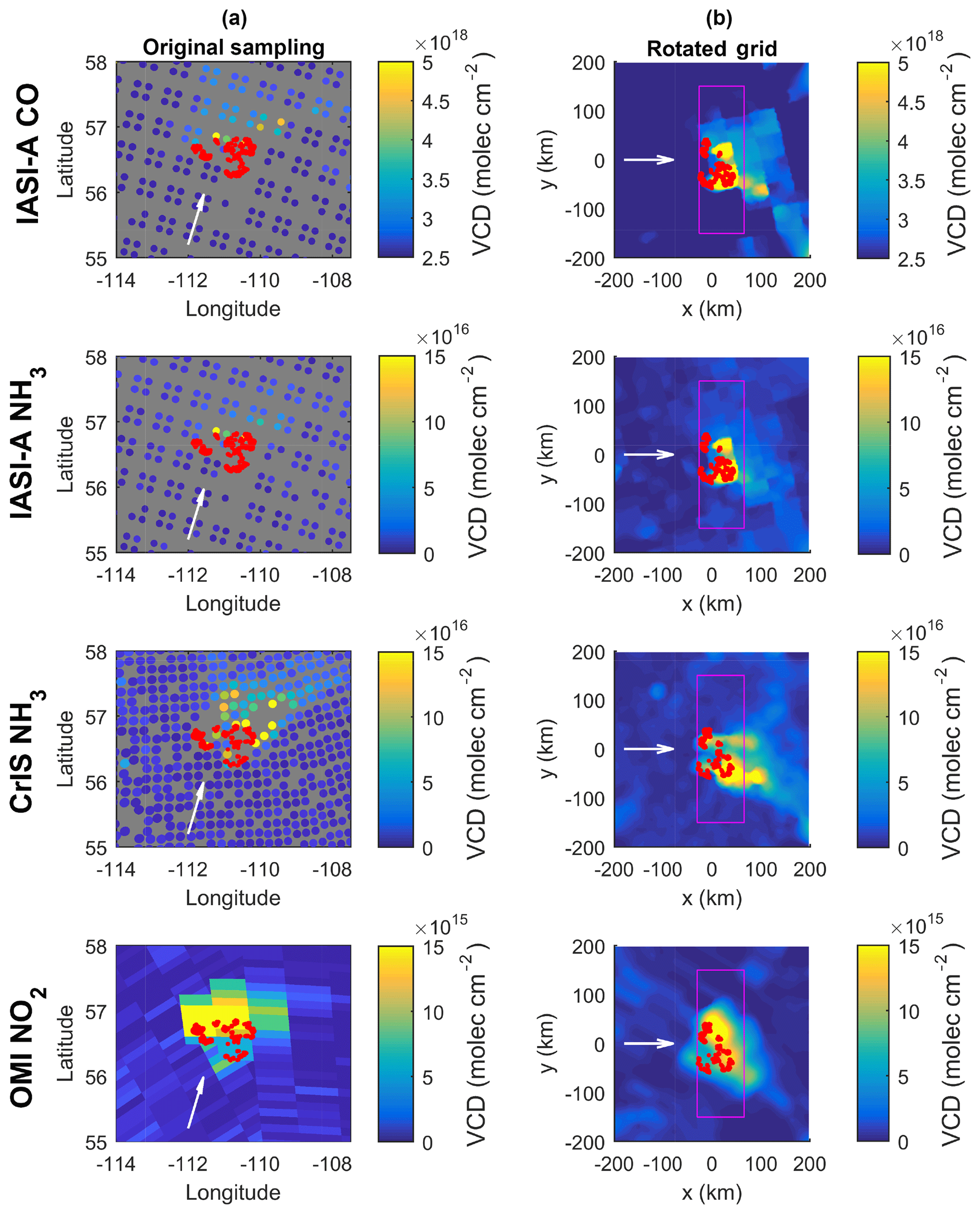
Figure 1Example of the analysis methods for 16 May 2016, with MODIS fire hotspots indicated (red dots). (a) Satellite data are shown with original pixel sampling, with the ECMWF wind direction indicated by the white arrow. (b) Data are gridded and oriented so that +x is downwind. The pink rectangles indicate the area over which the emissions are calculated.
Figure 1 shows the original sampling of the satellite data and the smoothed, rotated data for 16 May 2016. Satellite data for the given day were oversampled onto the 4×4 km2 grid described above. For each VCD measurement, all grid points that were within the satellite pixel were assigned to that VCD value. This yielded vectors of oversampled latitude, longitude, VCD, and weights. These data were then averaged onto the 4×4 km2 grid using an averaging radius of 15 km and weighting the measurements by the inverse of the pixel area. Days with large gaps in gridded VCDs in the area of the fire hotspots and downwind of the fires were excluded from the analysis. This was done by visually inspecting the original and gridded VCDs for each day; if gaps in the data covered large areas that were required to resolve the plume or led to interpolation of the plume that looked suspect, the day's data were excluded. Most of the days excluded were missing more than half of the data over or downwind of the fire hotspots. For days with sufficient data, small gaps in the gridded dataset were filled using interpolation with the inpaint_nans function in MATLAB (D'Errico, 2009).
The baseline VCDs were subtracted from the daily VCDs, yielding dVCD, the portion of the VCD from fire emissions. Baseline VCDs were calculated using data from May 2014, a year and month not strongly affected by forest fire smoke, and the data were filtered to remove peak values (>99 percentile). For each day in 2016, background was estimated using the filtered data for the entire month of May 2014, which was oversampled, gridded, and rotated using the winds for the day in 2016, as described above. This was done so that baseline values which varied spatially due to, e.g., emissions from the oil sands were accounted for. For CO and NH3, the baseline VCDs did not have a strong systematic variation over the measurement area, as demonstrated by the mean and 1σ of the May 2014 VCDs, which were filtered to remove peak values (>99 percentile). For CO, mean and 1σ baseline values had small variability and were consistent across IASI instruments, with values of molec cm−2 for IASI-A morning, molec cm−2 for IASI-A evening, molec cm−2 for IASI-B morning, and molec cm−2 for IASI-B evening. The CO baseline VCDs are significant compared with the enhanced levels of CO within the plume ∼ 3–5×10¹⁸ molec cm−2. For IASI NH3, background values were molec cm−2 for IASI-A morning, molec cm−2 for IASI-A evening, molec cm−2 for IASI-B morning, and molec cm−2 for IASI-B evening. These values have more variability compared with CO and show biases between IASI instruments, but they are small (∼5 %) compared with the enhanced VCDs observed over the smoke plume of ∼ 5–15×1016 molec cm−2, and therefore any systematic differences will have a small influence on the emission estimates. The baseline VCDs for CrIS are larger than for IASI, with values of for day and for night. The differences between baseline VCDs for CrIS and IASI are due to differences in the retrieval methods, which affect results when VCDs approach zero. The baseline VCDs for NO2 reflect local emissions sources and ranged from 3 ×10¹⁴ molec cm−2 over remote regions to 2 ×10¹⁵ molec cm−2 over the minable oil sands region. The NO2 baseline values over the oil sands are of the same order of magnitude as the enhanced levels of NO2 in the plume ∼ 5–15 ×1015 molec cm−2. The 2014 baseline VCDs for NO2 were filtered for CRF < 0.3 and did not include any data affected by the row anomaly.
Next, boxes were drawn around dVCD, as shown for 16 May 2016 in Fig. 1. The width of the box in the crosswind direction, y, was ±150 km from the centre of the fire hotspots. This was large enough to encompass the plume up to 200 km downwind of the fire, as determined by examining VCD maps for each day. Upwind, −x, the top of the box was set to the first grid value to encompass all of the fire hotspots. Downwind, +x, the box was drawn 20 km downwind of the most downwind hotspot to ensure that all of the hotspots were enclosed in the box when accounting for the satellite footprints.
Within the box, emissions were calculated using Eq. (5). The mass, m, of CO, NH3, or NO2 in the box was calculated by integrating gridded dVCDs within the box and multiplying by the molecular mass of the species. tc was calculated from u, the mean downwind wind speed, and xc, the distance to the centre of the fires (or the centre of the grid). The mean downwind wind speed was calculated using ECMWF ERA5 winds at the pixels of the satellite measurements within the box. The wind profiles were interpolated to the satellite measurement locations, and the weighted average of winds over the vertical profile of the assumed plume shape was calculated. At each satellite pixel location, the component of the wind speed in the downwind direction was taken. Then the average of the downwind wind-speed components was calculated. τ was calculated from the data by examining the decay curves of NO2 and NH3 downwind of the fires, as described in Sect. 4.3.
The uncertainties associated with the emission estimates were calculated from a series of sensitivity tests. These tests were intended to determine the sensitivity of the emissions to different choices, which we have labelled as analysis settings, for the method, the plume shape, species lifetimes, handling the effect of smoke, the conversion of NO2 to NOx, and the diurnal variation of emissions. The calculated sensitivities provide at least a rough estimate of the uncertainty in the emission estimates. The subsections below describe how each analysis setting was chosen and how associated sensitivity tests were performed. In order to run the sensitivity tests described, emission estimates were recalculated using the alternate settings for days with sufficiently large emission estimates for the default settings (> 50 kt for CO; > 1 kt for NH3; > 0.5 kt for NOx). The estimated uncertainty was the mean percent difference in emissions between the sensitivity test and the default settings across all days. In addition to the sensitivity tests, the uncertainty in VCDs due to satellite retrievals was also accounted for. Table 1 summarises the analysis settings and associated uncertainty for CO, NH3, and NOx emission estimates. The total uncertainty in emission estimates, calculated by adding the various uncertainty terms in quadrature, was 67 % for IASI CO, 82 % for IASI NH3, 74 % for CrIS NH3, and 73 % for OMI NOx.
Table 1Summary of analysis settings and associated uncertainty for satellite emission estimates.

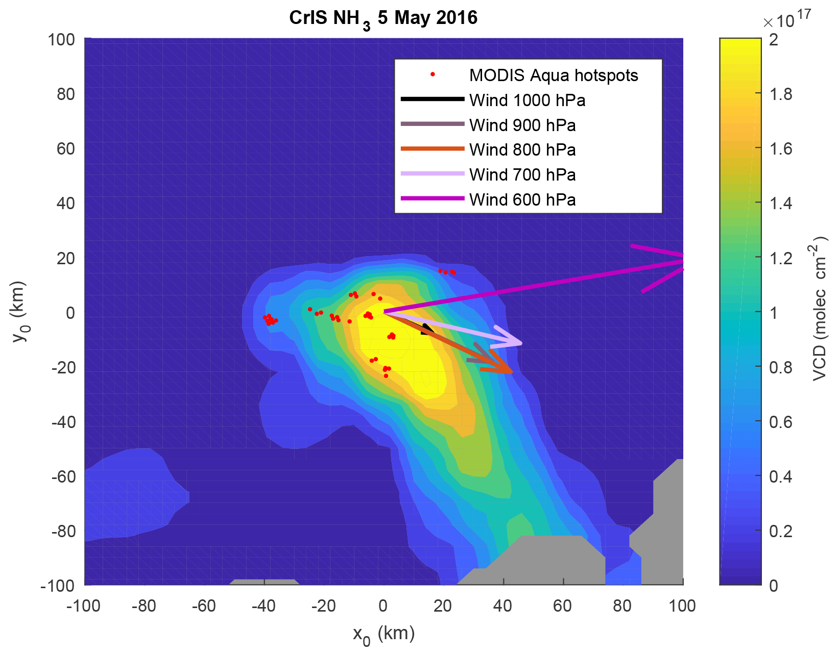
Figure 2Gridded CrIS NH3 VCDs on 5 May 2016, with MODIS Aqua fire hotspots (red dots) and ERA5 wind directions at various altitudes (arrows). Note that VCD data are presented in an unrotated frame of reference.
3.2 Method uncertainty
In order to estimate the uncertainty due to the selected emission estimate method, an alternate method was tested using IASI CO based on one-dimensional fluxes downwind of the fire. For the long lifetime of CO, Eq. (3) reduces to . The downwind flux emission estimate was calculated 4 km downwind of the fire using the line density L(x) and the downwind wind-speed components. It yielded emission estimates that were on average 48.8 % lower than the rectangular integration method. Similar values were obtained for one-dimensional flux calculations at 20 km downwind. The rectangular integration method (Eq. 5) was used in this study instead of the downwind flux method because rectangular integration includes the highest measured values of CO, NH3, and NO2 right over the fire hotspots. Furthermore, the rectangular integration method is less sensitive to the assumed lifetime of NO2 and NH3 than the one-dimensional flux method. Note that the size of the rectangle used for the rectangular integration method was also varied to test method uncertainty, but had a relatively small influence (∼ 5 %) on the emission estimates. The value of 48.8 % method uncertainty was used for both NH3 and NOx because the alternate method used in the sensitivity tests is based on downwind flux, whereby NH3 and NOx line densities are smaller due to their short lifetimes. Therefore, the alternate method is very sensitive to the assumed lifetimes and is therefore not appropriate for these species.
3.3 Plume profile shape
The smoke profile shape is used to weight the ECWMF wind profiles used in the flux calculations. For example, if the plume is at the surface, surface winds will dominate the flux calculations. If the plume is aloft 2–4 km, then winds at 2–4 km, which are typically larger than the surface winds, will be more important. Therefore, higher wind speeds lead to larger emission estimates through Eq. (5), where . In order to infer the shape of the plume profile, several datasets were used, including surface monitoring, satellite, and models, as described in the paragraphs below.
Surface air monitoring stations in the Fort McMurray area were affected by the plume and recorded enhanced levels of many parameters, including PM2.5, SO2, NOx, black carbon, NH3, and CH4, at locations both very near the fire and downwind (Landis et al., 2018). This suggests that the smoke profile reached the surface and was not strictly aloft. Therefore, all plume profile shapes tested extended to the surface.
On 5 May 2016, the wind directions varied with altitude and were compared against CrIS NH3 VCDs to infer the plume altitude range, as shown in Fig. 2. CrIS NH3 was the only VCD dataset with sufficient sampling to resolve the downwind shape of the plume on this day. The VCDs were gridded on a 4×4 km grid centred at the fire hotspots, which was not rotated. The ECMWF winds within a 40×40 km2 box around the fires were averaged, yielding the wind directions shown in the figure. The direction of the NH3 plume aligns best with winds between 1000 and 800 hPa (approximately 0–2 km), suggesting that the bulk of the NH3 plume is within this altitude range.
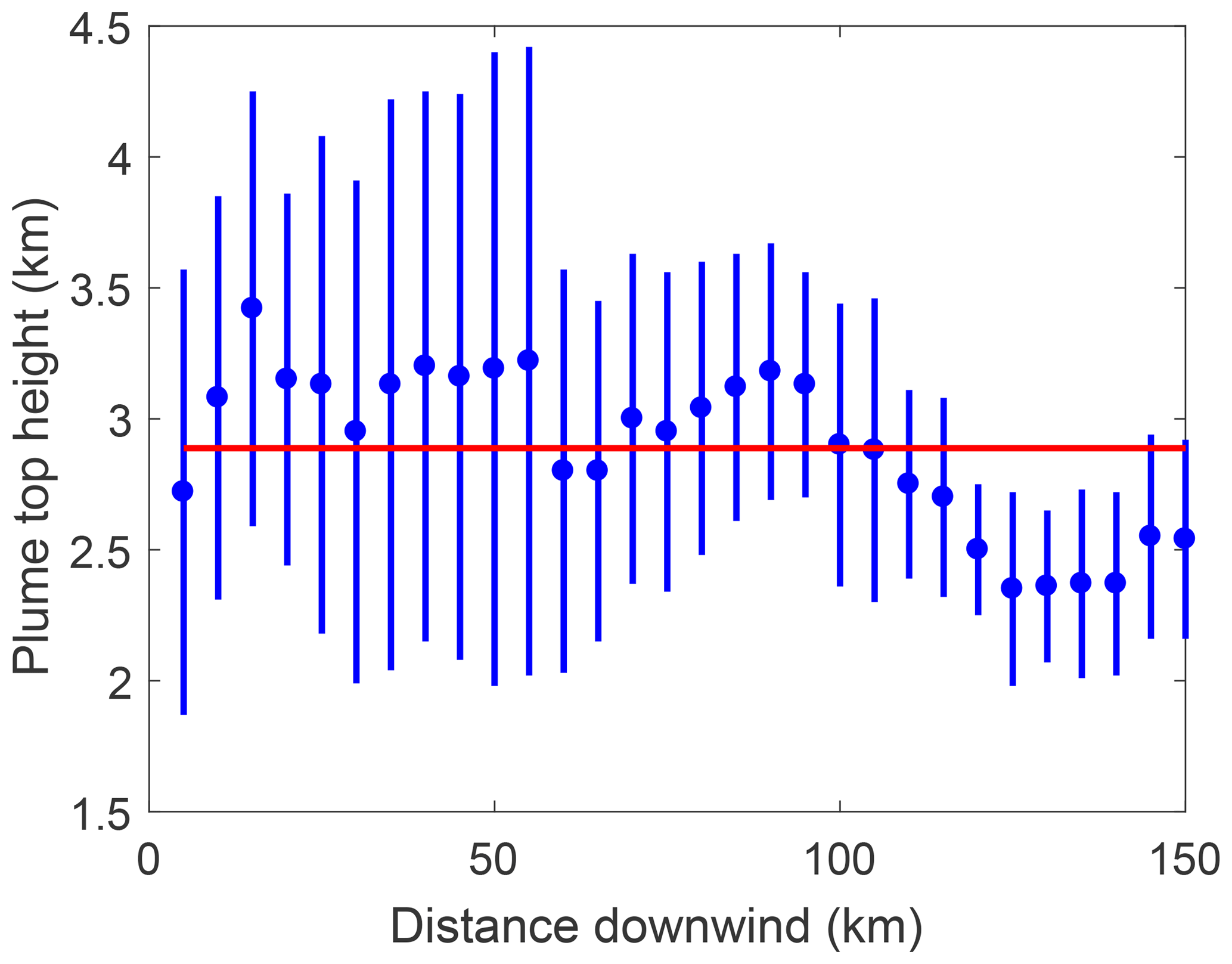
Figure 3MISR plume top height binned by distance downwind of the fire with 1σ standard deviation given by the error bars. The red line indicates the mean of the binned plume top height values (2.9 km).
Two additional satellite datasets and a model dataset were considered in order to estimate the altitude of the plume top. Smoke plume heights were retrieved using the NASA Multi-angle Imaging SpectroRadiometer (MISR) Interactive Explorer (MINX) software (Nelson et al., 2013). MINX uses imagery obtained from the MISR instrument's nine multi-angled cameras to perform the stereoscopic retrieval of heights and motion vectors for smoke plumes. A stereoscopic height retrieval algorithm was developed to focus specifically on aerosol plumes at the highest spatial resolution possible with the MISR data. This algorithm relies on the manual determination of smoke plume locations, boundaries, and wind directions. Nine distinct smoke plumes were visible by MISR over Fort McMurray during the month of May 2016 and were sampled over four days (4, 6, 15, and 18 May). All available pixels within the nine smoke plumes were binned over the distance downwind of the fire, as shown in Fig. 3. MISR plume heights within 100 km downwind of the centre of the fire were ∼3 km above sea level. Plume heights were also measured by the Cloud–Aerosol Lidar and Infrared Pathfinder Satellite Observations (CALIPSO), which passed over the wildfire area on 14 and 15 May, using the vertical feature mask (VFM) dataset (Winker et al., 2009). For measurements identified as “smoke”, the mean plume height within 110–112∘ W and 55–59∘ N was 2.9±0.2 km (N=18) on 14 May and 3.0±0.1 km (N=81) on 15 May; the error range denotes the standard deviation of the mean and N is the number of measurements in the average. Therefore, both the MISR and CALIPSO satellite datasets suggest that the plume reached a maximum altitude of ∼3 km. The GFAS model also calculates information on plume altitude using a plume rise model (Rémy et al., 2017). For the Horse River fire, daily average plume tops ranged from ∼2–4.5 km, while the mean altitude of maximum injection ranged from ∼1–3 km.

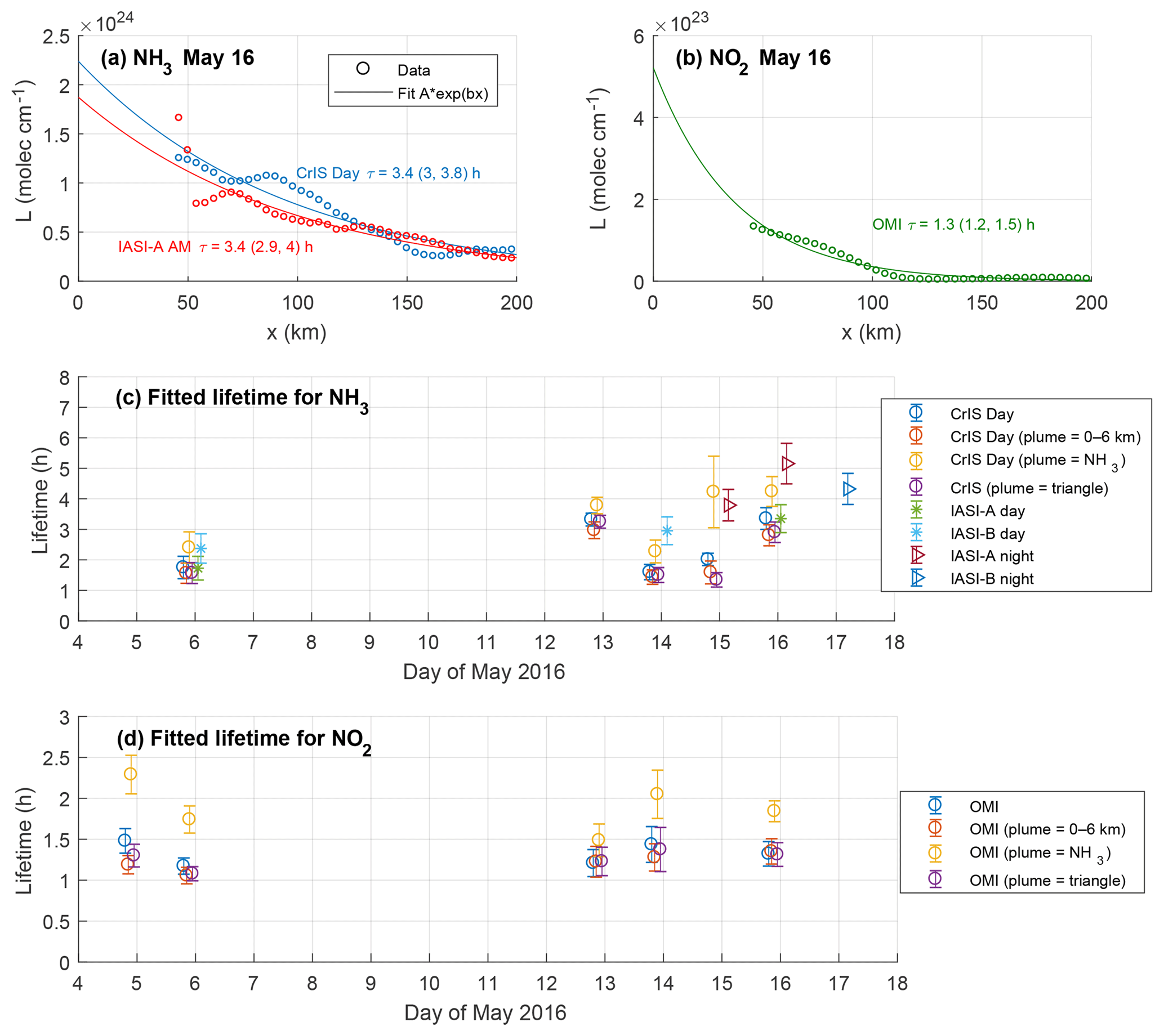
Figure 5Fitted lifetimes for NH3 and NO2. Example of fits on 16 May for (a) NH3 from IASI morning and CrIS daytime and (b) NO2 from OMI, with lifetime fit and 95 % confidence intervals given in the text box. Lifetimes and 95 % confidence intervals from fits for (c) NH3 and (d) NO2. Note that in panels (c) and (d) markers are offset from each other on the x axis to improve the readability of the figure.
Given the uncertainties in the shape of the plume profile, several plume shapes were considered in sensitivity tests for this analysis, as shown in Fig. 4. A box-shaped plume for 0–3 km was selected as the default setting, since most of the datasets considered suggest that the plume was within this altitude range. In addition, a box-shaped plume extending from 0–6 km was selected to account for higher possible plume heights. The “NH3 profile” plume shape was derived from the mean CrIS daytime NH3 profile during the fire for VCDs greater than 8 ×10¹⁶ molec cm−2 and is weighted more heavily toward the surface. The NH3 profile shape captures the possible contribution of residual smouldering to emissions, which are not lofted into the plume and may stay near the surface. The triangle plume shape peaks at ∼ 2 km and was calculated from climatological May smoke injection profiles for latitudes of 54–60∘ N and longitudes of 100–120∘ W (Sofiev et al., 2013), which are publicly available at http://is4fires.fmi.fi/ (last access: 21 February 2019). For all species, the largest difference in emission estimates from the default plume were obtained when adopting the NH3 profile plume shape, and therefore this shape was used to determine the uncertainties in Table 1. The emission estimates for CO are more sensitive to the plume profile shape than the emission estimates for NH3 and NO2. This is because for long lifetimes τ≫tc, Eq. (5) reduces to , and therefore the emission estimate is directly proportional to the plume wind speed, u.
3.4 Lifetimes of CO, NH3, NO2
The lifetimes of CO, NH3, and NOx within wildfire plumes affect emission estimates through Eq. (5). Previous satellite studies have assumed lifetimes of ∼ 1–2 weeks for CO (e.g., Whitburn et al., 2015), which is much longer than the ∼ 1–5 h timescale for the plume to clear the box used to estimate emissions in the present study. Therefore, a 2-week lifetime was used in the calculations, but the effect of varying this lifetime to, e.g., 1 week or infinity is negligible and not included in the error budget. For NH3, previous satellite emission estimate studies assume lifetimes of 12–36 h (Whitburn et al., 2015, and references therein) and Lutsch et al. (2016) estimated a lifetime of 48 h using a ground-based FTIR. However, those studies use methods which average over longer time periods and therefore consider NH3 further downwind than in the present study. Closer to the emission source, lifetimes could be shorter (Paulot et al., 2017). For example, aircraft observations in a smoke plume near a wildfire in the Alaska boreal forest found that NH3∕CO decreased by 1∕e in 2.5 h (Goode et al., 2000). Aircraft observations over chapparal fires in California found that NH3∕CO decreased by half in 4.5 h (Akagi et al., 2012), corresponding to a lifetime of ∼6 h, but most of the decrease in NH3∕CO occurred in the first hour, suggesting rapid initial loss of NH3. For satellite-derived NOx emission estimates, Schreier et al. (2015) assumed a 6 h lifetime based on satellite measurements over megacities (Beirle et al., 2011). Mebust et al. (2014, 2011) used a shorter lifetime of 2 h based on several observations of lifetimes in plumes ranging from 2 to 3 h. Tanimoto et al. (2015) calculate two alternate sets of emissions for NO2 using both lifetimes of 2 and 6 h.
For the present study, lifetimes of NH3 and NOx were estimated directly from the satellite VCD datasets, as shown in Fig. 5. For each day with sufficient data, the line density of NH3 and NO2, L(x), as a function of downwind distance from the centre of the fire hotspots, x, was calculated. L(x) was calculated using data within ±150 km crosswind. Based on Eq. (3), an exponential was fitted to the L(x) curve in order to calculate the lifetime τ, as shown on 16 May. Then, using the exponential fit parameter and the weighted-average wind speed of the plume, u, the lifetime, τ, was calculated. The fitted lifetimes are also shown in Fig. 5, with error bars denoting the 95 % confidence intervals of the exponential fit parameter. Lifetimes are only shown for days with sufficiently large plumes (emissions > 1 kt d−1 for NH3 or > 0.5 kt d−1 for NOx) and small fitting errors (< 1 h for both NH3 and NO2). Approximately 60 % of ammonia fits with sufficiently large plumes did not meet the fitting error criteria; this occurred primarily when wind speeds were low and/or winds were variable downwind, and therefore the plume changed direction and/or accumulated over some downwind locations. All NO2 fits met the fitting criteria, as the short lifetime of NO2 makes it less sensitive to inconsistencies in the winds far downwind. The fitted lifetimes were calculated using wind speeds from both the 0–3 km box profile shape and the alternate wind profile shapes shown in Fig. 4. The plume weighted toward the surface (NH3 profile) yielded longer lifetimes due to lower wind speeds. Note that the effect of other parameters included in the sensitivity tests, such as NO2 AMFs, were also tested but had a very small impact on the fitted lifetimes.
Based on the fitted lifetimes, values of τ=3 h for NH3 and τ=1.5 h for NO2 were used in this analysis. The NH3 lifetime of 3 h is much smaller than the other satellite emission studies described above, but is reasonable given that the emission estimate method considers NH3 very near the emission source, where lifetimes could be shorter. For the sensitivity tests, minimum values of 1.5 h for NH3 and 1 h for NO2 were derived from the lower range of the fitted lifetime values. For NH3 and NO2, upper-range values of 12 and 6 h were based on the satellite-derived emission studies described above. Sensitivity tests were run for both the upper- and lower-range values; the largest deviation from the default setting was used to estimate the uncertainty. For NH3, the uncertainty due to the lifetime is 47.9 % based on the 1.5 h lower-range lifetime; for NO2, the uncertainty is 34.9 % based on the lower-range value of 1 h. This is larger than the sensitivity calculated by Mebust et al. (2011) because, although the emission estimate methodology is similar, a larger range of possible lifetimes is used in the present study. Other emission estimate methods can yield larger sensitivity to lifetime; for example, Tanimoto et al. (2015) found that NOx emission estimates vary by a factor of 2–3 depending on whether a 2 or 6 h lifetime was assumed when working from monthly average gridded satellite NO2 measurements.
3.5 Effect of smoke on VCDs
At infrared wavelengths, smoke aerosol does not have a strong effect on retrievals. Clarisse et al. (2010a) showed the impact of biomass burning aerosol on IASI retrievals in the 800–1200 cm−1 range and found the strongest effect for 1000–1200 cm−1. IASI NH3 is retrieved in the 800–1200 cm−1 range, but most of the weight is for 900–980 cm−1. CrIS retrievals are performed for 650–1095 cm−1, with the main NH3-absorbing spectral region at 960–970 cm−1. The effect of biomass burning for 900–980 cm−1 is small (Clarisse et al., 2010a) and therefore will have minor influence on the IASI and CrIS NH3 retrievals. IASI CO retrievals are performed in the 2128–2206 cm−1 wavelength range in which the effect of aerosol is also weaker than in the 1000–1200 cm−1 range (Sutherland and Khanna, 1991). Therefore, uncertainties due to the effect of smoke on the VCDs are insignificant compared to other sources of error and were not included in the uncertainty calculations for IASI and CrIS.
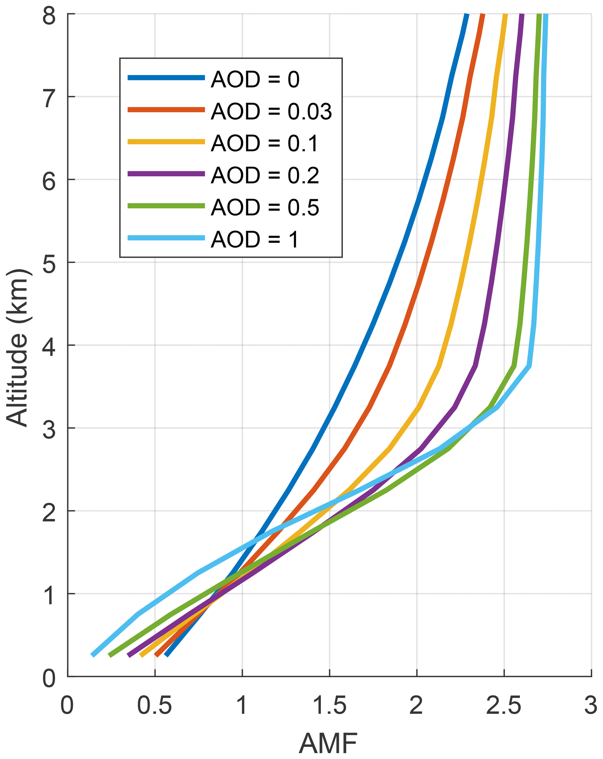
Figure 6Example AMFs as a function of altitude for various AODs for a 0–3 km smoke plume. AMFs are shown for clear skies above the plume. SZA: 30∘, viewing zenith angle: 50∘, albedo: 0.03, surface pressure: 1000 hPa, and column ozone: 350 DU.
OMI measurements are taken at UV–visible wavelengths, and therefore the scattering of sunlight to the instrument is affected by the smoke plume. The ECCC AMFs (McLinden et al., 2014) are calculated assuming no aerosol is present. To account for the smoke, AMFs were recalculated using the same inputs but with an aerosol profile present as defined by a profile shape, a total aerosol optical depth (AOD), refractive index, and size distribution. The refractive index (1.5+0.01i) (Dubovik et al., 2000) and size distribution (log-normal; r=0.1 µm, σ=0.3) were fixed. A default profile shape with constant number density (or extinction) between 0 and 3 km was used, although other profile shapes were also tested. AMFs were then calculated for AODs of 0, 0.03, 0.1, 0.2, 0.5, and 1. Figure 6 shows sample AMF profiles for various AODs assuming a 0–3 km smoke plume. For larger AODs, sensitivity to the surface is somewhat reduced and sensitivity to layers of the atmosphere above 1–2 km is somewhat higher.
The original (ECCC) NO2 VCD was then used as a proxy for smoke AOD using a relationship derived during the BOReal forest fires on Tropospheric oxidants over the Atlantic using Aircraft and Satellites (BORTAS) campaign (Bousserez et al., 2009):
where VCD molec cm−2 and cm2 molec−1. Interpolating between the various precalculated AOD-AMF tables, the AMF corresponding to the AOD was found and used to recalculate the VCD.
The OMI NO2 emission estimates using the smoke AMFs were compared against emission estimates using the typical aerosol-free CRF-based AMFs and yielded emission estimates that were 15.1 % smaller than the CRF-based AMFs. Alternative smoke AMF profiles were also tested using the triangle plume profile (Fig. 4), but the change in the plume profile did not have as significant of an effect on the results (< 5 % difference in emission estimate sensitivity tests). Therefore, uncertainty in AMFs was set at 15.1 % in Table 1. The relatively modest impact of the smoke on the AMF is a result of offsetting effects. There was a significant reduction in AMF due to the combination of aerosol and weighting of the NO2 profile towards the surface, but this was offset by using a CRF of zero whenever the original VCD exceeded 1×10¹⁵ molec cm−2. In all cases, the shape of the aerosol profile matched that of the NO2 profile.
3.6 Conversion of NO2 to NOx
In order to convert the NO2 emission estimates from OMI to NOx, a factor of NO2∕NOx of 0.8 was used. This was based on an average of over 40 wildfire plumes in Alberta and Saskatchewan in 2017 using the FireWork emissions simulation with the Global Environmental Multi-scale – Modelling air quality and Chemistry (GEM-MACH) chemical transport model. Within 100 km downwind of the fire, the modelled ratio was found to be 0.8 and is consistent with measurements of NO2∕NOx at the Fort McMurray surface air monitoring stations. Other studies of NOx emissions from plumes have used values of 0.75 (Schreier et al., 2014; Tanimoto et al., 2015) and 0.7 (Mebust and Cohen, 2014; Mebust et al., 2011). Therefore, the uncertainty due to conversion from NO2 to NOx in Table 1 was set to 10 %. Note that NOx emissions are presented as mass of NO throughout this paper.
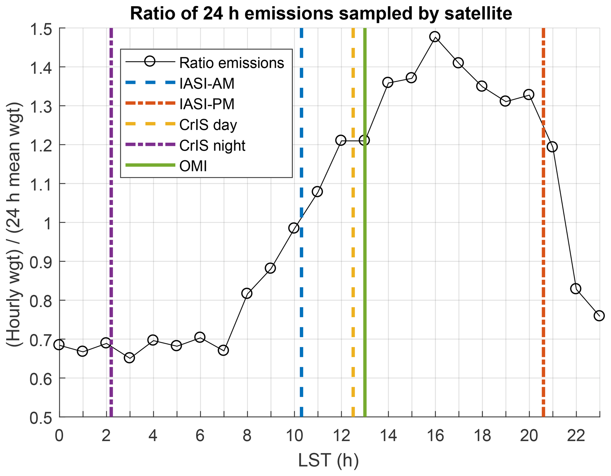
Figure 7Ratio of 24 h emission rates sampled by satellite at various LST. The y axis shows the ratio of the hourly emission weight over the 24 h mean emission weight. The typical overpass times for the IASI, CrIS, and OMI satellites over the Horse River fire area are also shown.
3.7 Diurnal variation of emissions
Emissions from wildfires vary diurnally, with more active burning and larger emissions typically occurring during the daytime. The satellite instruments measure emissions at a fixed time of day, depending on the satellite's orbit, which is assumed in this study to represent the daily average emission rate. In order to estimate uncertainty due to the diurnal variation of emissions, the diurnal weight profile from the Western Regional Air Partnership (2005), which is used in the FireWork model, was considered. Figure 7 shows the hourly weight divided by the 24 h weight plotted as a function of LST, with the satellite overpass time indicated. Note that the satellite overpass time does not coincide exactly with the time of the measured emissions; VCDs measured both over the hotspots (approximately at the time of emission) and downwind (typically ∼ 1–2 h after emission) are used together to estimate emissions. Emissions are at a minimum overnight and therefore the CrIS night-time overpass samples approximately 0.7 times the 24 h average. Over the course of the morning, emission rates increase. Measurements taken during the IASI morning overpass are approximately equivalent to the 24 h average. By afternoon, emission estimates at the CrIS and OMI overpass times are 1.2 times the 24 h average. At the IASI evening overpass time, emission estimates are similarly 1.2 times the 24 h average. Based on this diurnal profile, an uncertainty of 20 % was assigned for the diurnal variation of emissions.
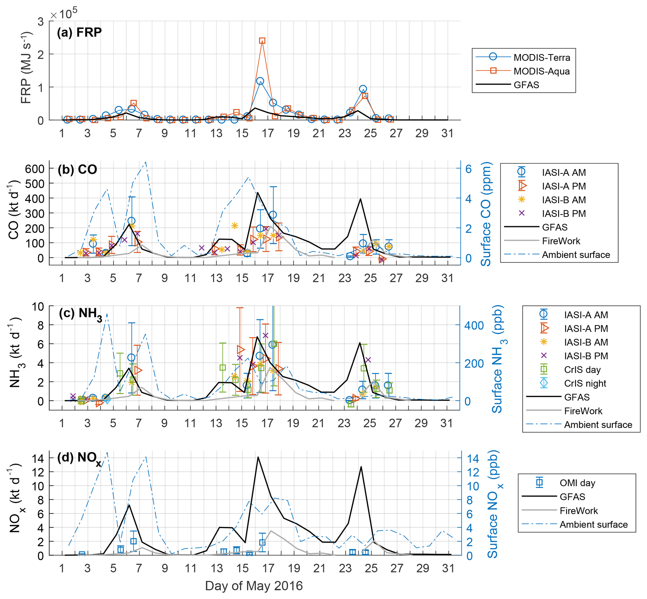
Figure 8Time series of (a) FRP and emission estimates and surface concentrations for (b) CO, (c) NH3, and (d) NOx from satellite, models, and air monitoring stations. Note that error bars are not shown for IASI-B emissions to improve the readability of the figure. The surface concentrations are the 24 h average concentrations of CO at the Fort McMurray–Athabasca Valley air monitoring station and NH3 and NOx at the Fort McMurray–Patricia McInnes air monitoring station. Note that NOx measured at Fort McMurray–Athabasca Valley shows similar variability, but is not shown here.
3.8 VCD from satellite retrievals
Uncertainties in the satellite VCD retrievals were also included in the total uncertainty. The emission estimates are directly proportional to the mass, which is calculated from the VCDs (Eq. 5), and therefore the percent uncertainty in the satellite VCD was applied directly as an uncertainty term. Note that this is based on the assumption that the satellite VCDs include systematic uncertainties that do not cancel out as data are averaged. For IASI CO, a VCD uncertainty of 35 % was estimated based on comparisons between IASI and ground-based spectrometers under fire conditions (see Sect. 2.1). IASI NH3 VCDs are ∼ 40 % lower than ground-based FTIR VCDs (Dammers et al., 2017). CrIS NH3 VCDs have very little bias compared with FTIR (∼ 0–5 %) (Dammers et al., 2017) and therefore the VCD total error in the retrievals was used; for enhanced VCDs (greater than 2 ×10¹⁶ molec cm−2) within a box around the fires (55–58∘ N and 108–114∘ W), the mean VCD total error was 16.5 %. For OMI NO2, estimated uncertainties are 30 % over polluted areas with clear-sky conditions (Bucsela et al., 2013). Uncertainties in OMI VCDs due to the smoke plume have been calculated separately in Sect. 4.4.
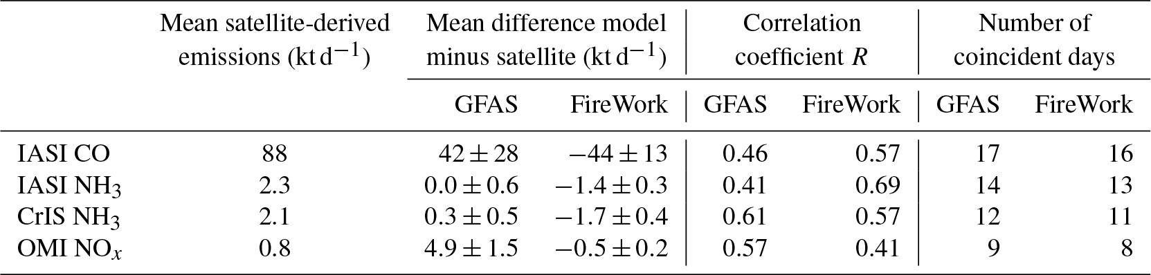
Table 2Comparison statistics for emission estimates from satellite versus models. Uncertainty in the mean difference is the standard error.
4.1 Time series of emission estimates and comparison with models
Figure 8 shows the time series of FRP and emission estimates for CO, NH3, and NOx from satellite and from the GFAS and FireWork models during the Horse River fire. The FRP is shown for the MODIS Terra (morning overpass), MODIS Aqua (afternoon overpass), and the GFAS model, which assimilates MODIS data. The FRP values from the MODIS overpasses have a similar day-to-day variability compared with GFAS, but have much larger peaks than the model. All three FRP datasets show three periods of active burning for approximately 5–8, 15–18, and 23–26 May. For CO and NH3, the satellite data agree within uncertainties with the modelled data. During the first active period (5–8 May), satellite emissions agree better with the larger emissions in GFAS. During the third active period (23–26 May), the satellite emissions are closer to the lower emissions from FireWork. During the second active period (15–18 May), satellite emissions are close to both the GFAS and FireWork models. For NOx, GFAS emissions are much larger than for OMI and FireWork. 24 h average surface concentrations of CO, NH3, and NOx in Fort McMurray are also enhanced during the active fire periods. The surface air monitoring data tracks somewhat with the satellite and model emission data, with similar periods of active burning. The air monitoring station observes a larger relative peak around 4 May, likely because the fire was active in Fort McMurray near the air monitoring stations at this time (MNP LLP, 2017). The smaller relative peaks in the surface air monitoring data for the third active period (23–26 May) are likely because the fire had moved to the east of Fort McMurray (MNP LLP, 2017) and was therefore further from the monitoring stations.
Table 2 shows statistics for the satellite emissions compared with the daily model output. Note that all available IASI emission estimates (IASI-A morning, IASI-B morning, IASI-A night, IASI-B night) were averaged daily, yielding single sets of IASI emission estimates for CO and NH3. The CrIS comparisons exclude the single night-time emission estimate. For CO, the satellite estimates fall between the GFAS and FireWork estimates, with GFAS biased high and FireWork biased low, both by ∼ 40 kt d−1. For NH3, emission estimates for GFAS and the satellite data agree well in magnitude, while the FireWork emission estimates are ∼ 1.5 kt d−1 lower than the satellite data. For NOx, GFAS estimates ∼ 5 kt d−1 more NOx than OMI, while FireWork emissions are much closer to the OMI measurements (within 0.5 kt d−1). For all three species (CO, NH3, and NOx), the Pearson correlation coefficients are between 0.41 and 0.69 between satellite data and both models.
4.2 Emission ratios: relationships between CO, NH3, and NOx
Figure 9 shows the relationships between CO, NH3, and NOx in the satellite and model emission estimates and surface air monitoring station data. The surface air monitoring station and MAML measurements are shown for May 2016 only and are presented as a mass (µg m−3) for consistency in ratios with emissions, which are calculated as a mass rate. Background levels were subtracted from the surface air monitoring concentrations. Background values were the mean of May measurements at the Fort McMurray and Fort McKay stations for 2013–2015, with hours influenced by wildfire smoke removed (Ross et al., 2018), and were 92 ppb for CO, 0.5 ppb for NH3, and 1 ppb for NOx. Note that NOx measurements with more than 10 ppb of NO were excluded from the scatter plots because they often occurred for very low CO concentrations and skewed the scatter plots. The high levels of NO indicate close proximity to an NOx source, perhaps due to nearby flaming of the wildfire or anthropogenic sources in Fort McMurray. The slopes for emission and ambient concentration ratios were calculated using a linear least squares fit that was constrained to go through the origin. The 95 % confidence intervals in the slope were calculated by bootstrapping the data using the bias-corrected and accelerated percentile method (MathWorks, 2018).

Figure 9Scatter plots of emissions (a, c, e) and surface concentrations (b, d, f) for NH3∕CO (a, b), NOx∕CO (c, d), and NOx∕NH3 (e, f). Daily emissions are shown for satellite and the GFAS and FireWork models. The differences in surface concentrations are hourly averages minus background concentrations. The slope and 95 % confidence interval (given in brackets) of a linear fit constrained to go through the origin are also shown in the legend.
Satellite emission ratios of NH3∕CO of 0.023 for IASI and 0.024 for CrIS are approximately 1.5 times larger than the modelled ratios. The MAML enhancement ratio of 0.042 is 2.5 times larger than the modelled ratios. Neither of the Fort McMurray air monitoring stations have collocated CO and NH3 measurements. Paulot et al. (2017) measured NH3∕CO emission ratios with IASI of 0.016–0.027 over Alaska, but noted that their values are biased low compared with the emission factors calculated in situ by 35 % because IASI measured older air masses. When scaled up by 35 %, these values are 0.024–0.040, which fits within the range of satellite and surface ratios reported here. R'Honi et al. (2013) measured NH3∕CO from IASI for wildfires over Russia and found that the ratio varied in time from 0.01 to 0.052, which spans the range of values calculated in the present study. With two ground-based FTIRs, Lutsch et al. (2016) measured NH3∕CO emission ratios of 0.0173±0.0014 and 0.0189±0.0018 at two locations for an assumed NH3 lifetime of 48 h over the long distances of the transport of the plume from fires in the Northwest Territories of Canada. These ratios are slightly lower than the values calculated in the present study; when Lutsch et al. (2016) assume a shorter lifetime of 36 h, emission ratio estimates at the two stations increase to 0.0471±0.0039 and 0.0311±0.0029 and are therefore in broad agreement with the values reported here.
For NOx∕CO, the FireWork and GFAS NOx∕CO emission ratios are 1.5 and 3 times larger, respectively, than the satellite emission ratio of 0.01. Similarly, for NOx∕NH3 mean ratios from FireWork and GFAS are 3 and 6 times larger, respectively, than the satellite emission ratios of 0.3–0.4. Enhancement ratios from surface stations are 0.003–0.004 for NOx∕CO and ∼ 0.06–0.08 for NOx∕NH3, which is much lower than the satellite and model values. This may be because of the weaker correlation between NOx, which is released primarily during flaming combustion, and NH3 and CO, which are released primarily during smouldering combustion. Furthermore, the lifetime of NOx is shorter than for NH3 or CO, and therefore NOx may have been lost prior to detection by the surface monitors. Simpson et al. (2011) measured NOx∕CO enhancement ratios for boreal forest fires during BORTAS and found values of 0.0024±0.0001 for NO2 and 0.0056±0.003 for NO, which falls between the surface monitoring values in the present study.
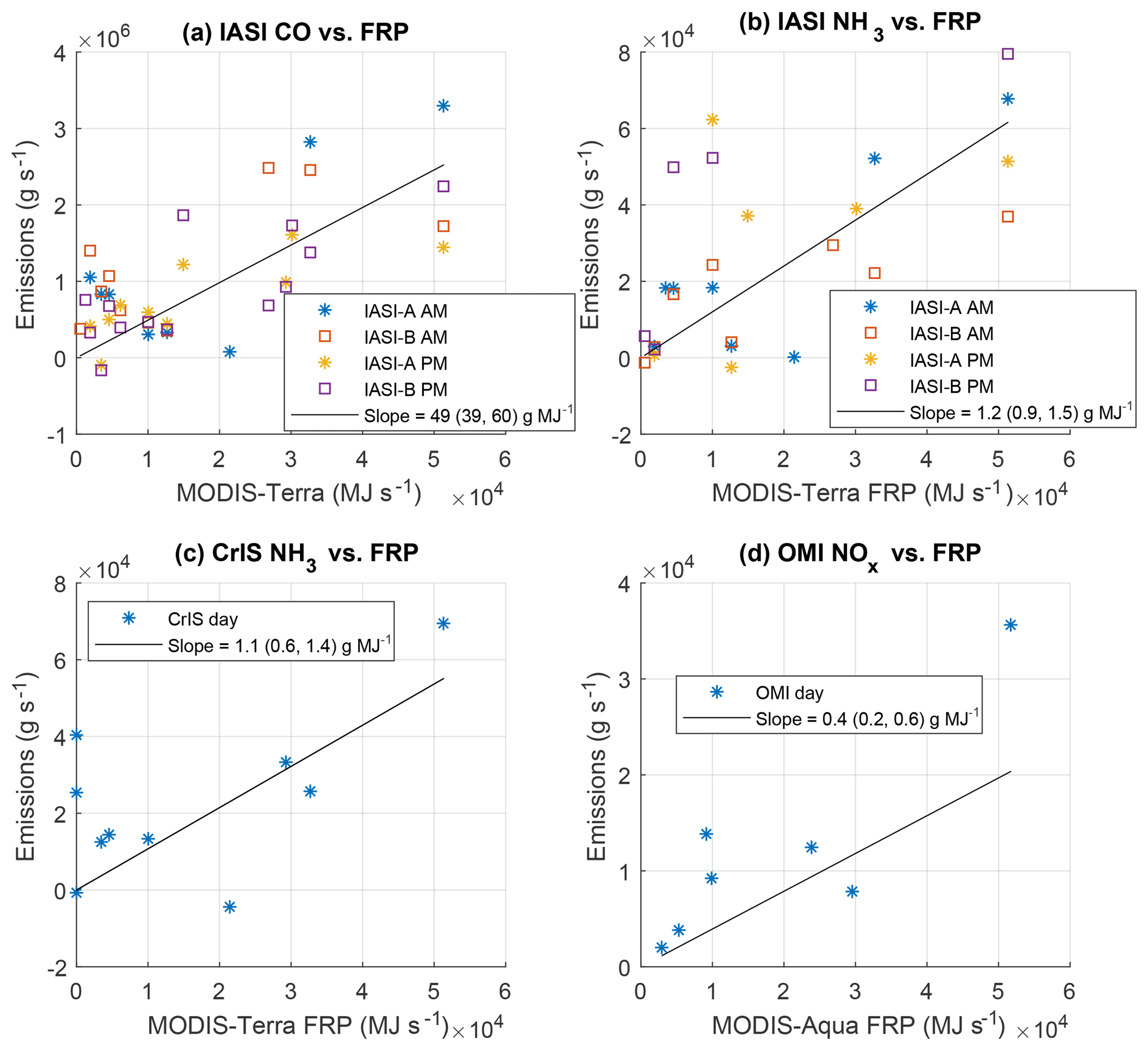
Figure 10Scatter plot of daily emissions versus MODIS FRP for (a) IASI CO, (b) IASI NH3, (c) CrIS NH3, and (d) OMI NOx. The slope and 95 % confidence interval of a linear fit constrained to go through the origin are also shown.
4.3 Satellite-derived emission factors
Emission factors can be estimated from satellite data by assuming a linear relationship between emission estimates and FRP and then applying a conversion factor to account for the relationship between FRP and fuel consumed (e.g., Mebust et al., 2011). The relationship between satellite emission estimates and MODIS FRP is shown in Fig. 10 for all available satellite emission estimates, except for the single CrIS night-time emission estimate. 16 and 24 May were excluded from the scatter plots and fits because the large peaks in the MODIS FRP on these dates do not correlate with similarly high values in the emission estimates (see Fig. 8), which causes reduced correlation (R=0.2–0.6). Correlation coefficients between the MODIS FRP and the satellite datasets range from R=0.59–0.86 when these dates are removed. The MODIS Aqua satellite (LST = 13:30) has the closest overpass time to CrIS (LST = 12:30), but the MODIS Aqua FRP did not correlate well with CrIS NH3 emissions (R= 0.02). Therefore, MODIS Terra was used instead (R= 0.59). This may be because the VCDs measured by CrIS are from emissions ∼ 1–2 h before the overpass time (see Sect. 4.6) and are therefore closer to the MODIS Terra overpass time (LST = 10:30). The slope of the emissions versus MODIS FRP yields the emission coefficient (g MJ−1). The slope was calculated using a linear least squares fit that was constrained to go through the origin. The 95 % confidence intervals in the slopes were calculated by bootstrapping the data using the bias-corrected and accelerated percentile method in MATLAB (MathWorks, 2018).
Table 3Emission factors from satellite, models, and previous studies. For the satellite data, 95 % confidence intervals from the emissions versus FRP fits are given in brackets. The FireWork emission factors are based on the mean ratio of flaming versus smouldering and residual burning for the Horse Rive fire.
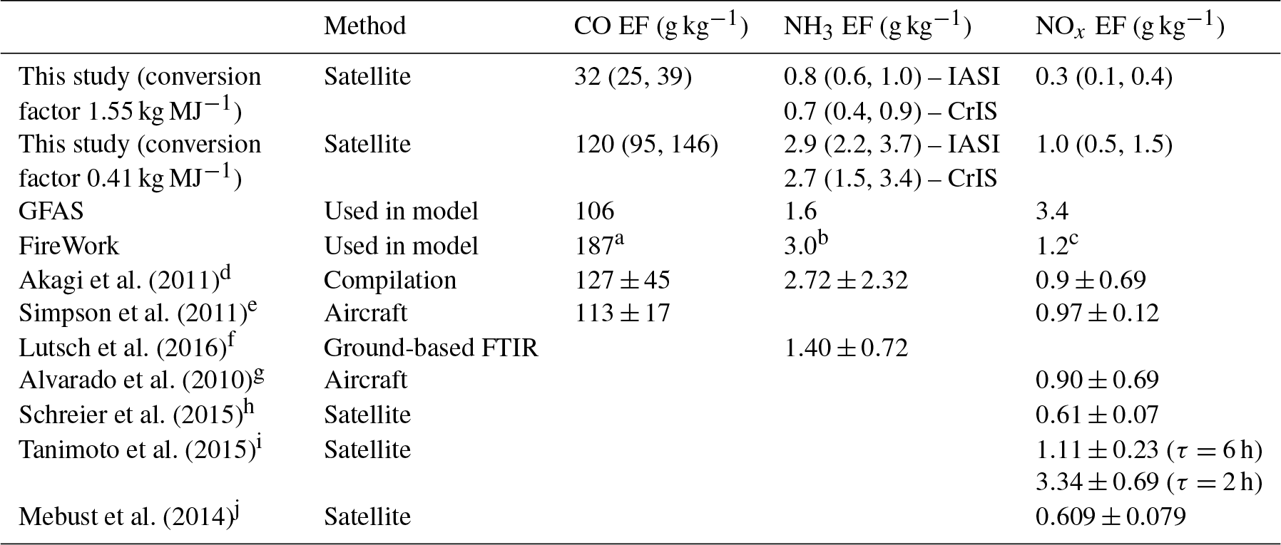
a From combination of CO EFs: flaming = 71.8 g kg−1; smouldering and residual = 210.12 g kg−1; b from combination of NH3 EFs: flaming = 1.21 g kg−1; smouldering and residual = 3.41 g kg−1; c from combination of NOx EFs: flaming = 2.42 g kg−1; smouldering and residual = 0.91 g kg−1; d Boreal forest; e plumes measured in Saskatchewan and Ontario, Canada; f plumes originating from Northwest Territories, Canada; g Plume in Alberta, Canada; h North American boreal forest; i Alaskan boreal forest; j global estimate for boreal forest.
The IASI CO emission coefficient was 49 g MJ−1 for IASI measurements. The NH3 emission coefficient was 1.2 g MJ−1 for IASI and 1.1 g MJ−1 for CrIS. The OMI NOx emission coefficient was 0.4 g MJ−1, with 95 % confidence intervals of 0.2–0.6 g MJ−1. Using satellite data over multiple fires, several other studies have calculated emission coefficients for NOx over large areas. Mebust and Cohen (2014) found a value of ∼ 0.3 g MJ−1 for the North American boreal forest using a similar method with OMI satellite data. Schreier et al. (2015) found a similar value for the North American boreal forest of 0.25±0.03 g MJ−1 using GOME-2 satellite monthly averages on a grid. These two values are within the 95 % confidence interval in this study. Tanimoto et al. (2015) found higher values of ∼ 1.7–5.2 g MJ−1, depending on the assumed lifetime of NO2, for the boreal forest in Alaska using monthly means of GOME and SCIAMACHY satellites on a grid.
A conversion factor can be applied to calculate emission factors (g kg−1) from emission coefficients (g MJ−1). Some satellite NOx emission studies (e.g., Mebust and Cohen, 2014; Schreier et al., 2015) use a single conversion factor of 0.41 kg MJ−1 proposed by Vermote et al. (2009) for all land types. The GFAS model, however, uses conversion factors which depend on the land cover type based on linear regressions between GFAS FRP and dry matter combustion rate from the GFED (Kaiser et al., 2012). The Horse River fire was primarily over extratropical forest with organic soil land cover type, with a GFAS conversion factor value of 1.55 kg MJ−1, which is ∼ 4 times larger than the 0.41 kg MJ−1 conversion factor. Since the conversion factors are applied directly to the emission coefficients, the choice of conversion factor can lead to emission factors that differ by a factor of ∼ 4. Therefore, two sets of emission factors were calculated for this study using the two different conversion factors.
Table 3 shows the emission factors calculated by satellite for both the 0.41 and 1.55 kg MJ−1 conversion factors and used in the GFAS and FireWork model datasets. The FireWork model uses separate emission factors for flaming, smouldering, and residual smouldering. The ratio of flaming ∕ smouldering + residual was 0.2 for the Horse River fire, as calculated using fuel consumption types from CWFIS. Effective FireWork emission factors for the Horse River fire were calculated using this ratio and the emission factors for flaming and for smouldering and residual burning. The emission factors for the boreal forest from Akagi et al. (2011), which are based on a compilation of studies and are used in the GFED model (Van Der Werf et al., 2017), and from other studies using ground-based FTIR, aircraft, and satellite are also included for comparison.
For CO, the satellite-derived emission factors are 32 g kg−1 for the 1.55 kg MJ−1 conversion factor and 120 g kg−1 for the 0.41 kg MJ−1 conversion factor. Emission factors from GFAS (106 g kg−1), the Akagi et al. (2011) compilation (127±45 kg), and the BORTAS aircraft measurements (Simpson et al., 2011) (113±17 g kg−1) all fall within this range and agree slightly better with the satellite-derived emission factor for the 0.41 kg MJ−1 conversion factor. The emission factor used in FireWork is a somewhat larger 187 g kg−1. To our knowledge, no previous studies have derived wildfire emission factors for CO using satellite.
For NH3, emission factors of 0.8 and 0.7 g kg−1 were derived for IASI and CrIS, respectively, using the 1.55 kg MJ−1 conversion factor. Using the 0.41 kg MJ−1 conversion factor, values of 2.9 g kg−1 for IASI and 2.7 g kg−1 for CrIS were calculated. Emission factors from other studies included in the table fall within the broad range of the satellite-derived values. The emission factors used in GFAS (1.6 g kg−1) and derived from ground-based FTIR (Lutsch et al., 2016) (1.40±0.72 g kg−1) are between the emission factors estimated for the two different conversion factors. The emission factors used in FireWork (3.0 g kg−1) and included in the Agaki et al. (2011) compilation (2.72±2.32 g kg−1) are within the confidence intervals for the satellite-derived values for the 0.41 kg MJ−1 conversion factor.
For NOx, the satellite-derived emission factors were 0.3 g kg−1 for the 1.55 kg MJ−1 conversion factor and 1.0 g kg−1 for the 0.41 kg MJ−1 conversion factor. Emission factors from the FireWork model (1.2 g kg−1), the Akagi et al. (2011) compilation (0.9±069 g kg−1), aircraft measurements in Alberta, Canada (Alvarado et al., 2010) (0.90±0.69 g kg−1), and the BORTAS aircraft campaign (Simpson et al., 2011) (0.97±0.12 g kg−1) all fall within this range. Previous satellite-derived values from Mebust et al. (2014) of 0.609±0.079 for boreal forests and Schreier et al. (2015) of 0.61±0.07 for North American boreal forests also fall within the range derived here. The GFAS NOx emission factor of 3.4 g kg−1 is higher than the satellite NOx emission factors, which is consistent with the large NOx emissions predicted by GFAS compared to satellite and FireWork (see, e.g., Table 2). The GFAS NOx emission factor is for extratropical forest, which includes both temperate and boreal forests. The inventory of Akagi et al. (2011) gives an emission factor for temperate forests of 2.51±1.02, which is much larger than the value of 0.90±0.69 for boreal forests. The GFAS emission factors are, however, within the range of values derived from satellite by Tanimoto et al. (2015) for the boreal forest in Alaska.

Figure 11Total emissions for the Horse River fire in May 2016 from satellite and models (blue), with total annual anthropogenic emissions for Alberta from the 2016 APEI (red). The error bars represent satellite emissions scaled by models to account for gaps in sampling. The APEI emissions have been converted so that they are expressed as kt of NO.
4.4 Total emissions from the Horse River wildfire
The total emissions from the wildfire were calculated from the sum of all emission estimates over all days in May 2016 for the satellite measurements and models, as shown by the blue bars in Fig. 11. Total IASI emissions were calculated using the daily average IASI emissions, as described above. The total CrIS NH3 emission estimate includes only the daytime CrIS measurements. The satellite total emissions are a sum of days with available data and are therefore likely underestimated. The 24 h emission estimates from the GFAS and FireWork models were used to estimate how gaps in sampling affect the total emissions (sum of all emissions from the Horse River fire in May 2016 divided by sum of emissions on days with valid satellite estimates). The larger of the two modelled sampling scale factors was applied to the satellite emissions as a possible upper-range value, which is indicated by the error bars on the bar chart. For comparison, the total annual anthropogenic emissions for Alberta, including both mobile and point sources in 2016, are also shown from the Air Pollutant Emissions Inventory (APEI) (ECCC, 2018) with red bars.
For CO, satellite estimates of total emissions are 1.5×10³ kt, which falls between the GFAS total emission estimate of 2.6×10³ kt and the FireWork total emissions of 0.9×10³ kt. The emissions from this fire are comparable to the total annual CO emissions from all anthropogenic sources in Alberta of 992.6 kt. Gaps in the dataset have a small effect on the satellite-derived total emissions, with the upper-range value of 1.7×10³ kt based on the modelled sampling scale factors.
Satellite estimates of total NH3 emissions are 30 kt for IASI and 29 kt from CrIS, which after it is scaled using model data for gaps (error bar) agrees with the total emissions estimated from GFAS of 40 kt. Total emissions of NH3 from FireWork of 16 kt are lower than the satellite and GFAS estimates. The satellite-measured NH3 emissions from the Horse River fire for May 2016 are approximately 1∕5 the magnitude of total annual anthropogenic emissions in Alberta in 2016 (134.8 kt).
For NOx, satellite-derived total emission estimates of 7 kt are of the same order of magnitude as FireWork total emissions of 16 kt, but are much smaller than the total emissions from GFAS of 84 kt. However, there are fewer valid days with satellite emission estimates for NOx, and therefore the modelled sampling bias is larger and more uncertain, with GFAS suggesting that 61 % of the total emissions were sampled by satellite and FireWork suggesting that only 19 % of total emissions were sampled by the satellite. Therefore, the total NOx emissions as estimated from satellite could be as high as 40 kt after applying the sampling correction. The total satellite emissions of 7–40 kt for May 2016 are about 1 %–7 % of the magnitude of total annual anthropogenic emissions in Alberta for the year 2016. The NOx emissions from the Horse River fire are, however, of the same order of magnitude as the largest point source emitter in the Canadian oil sands area, the Syncrude Upgrader, which emitted 14 kt of NOx in 2016 (ECCC, 2017).
Emissions of CO, NH3, and NOx from the Horse River fire were estimated using the IASI, CrIS, and OMI satellite instruments, building upon the method of Mebust et al. (2014). Our approach used satellite-derived estimates of lifetimes for NH3 and NOx of 3 and 1.5 h. Multiple datasets, including satellite (CrIS NH3, CALIPSO, and MISR) and surface measurements, were used to estimate the plume profile shape, which is used to weight the wind profiles for the emission calculations. Based on sensitivity tests, uncertainties in the daily emission estimates were 67 % for IASI CO, 82 % for IASI NH3, 74 % for CrIS NH3, and 73 % for OMI NOx. Emission ratios for NH3∕CO, NOx∕CO, and NOx∕NH3 were calculated from the satellite-derived and model emission estimates, and enhancement ratios were calculated from the surface concentration measurements. The ratios were compared with the literature. Broad agreement was observed for NH3∕CO. For NOx∕CO and NOx∕NH3, values ranged by a factor of 10, perhaps due to uncertainties in emission factors and the short lifetime of NOx.
Emission factors for CO, NH3, and NOx were estimated from satellite-derived emissions using the relationship between the daily satellite measurements and assimilated FRP from GFAS. There is large uncertainty in conversion factors, which could range from a global value of 0.41 kg MJ−1 (Vermote et al., 2009) or 1.55 kg MJ−1 (Kaiser et al., 2012), specific to extratropical forest with organic soil land cover type. Therefore, the range of satellite-derived emission factors was very wide when considering the range of possible conversion factors and confidence intervals in the fits relating FRP to emissions: ∼ 25–146 for CO, ∼ 0.4–3.7 for NH3, and ∼ 0.1–1.5 for NOx. For the most part, emission factors for the GFAS and FireWork models, the Akagi et al. (2011) compilation, and aircraft and ground-based FTIR studies all fall within or close to these ranges; the exception is the GFAS NOx emission factor of 3.4, which is much larger than the values calculated here. Similar results were found when comparing day-to-day emission estimates from the satellite and models, with general good agreement between model and satellite (within a factor of 2), except for a clear positive bias in GFAS NOx relative to FireWork and satellite emissions. The agreement between the satellite instruments, model, and emissions inventories is remarkable given the uncertainties in the satellite-derived emissions and the natural variability in emissions due to, e.g., vegetation and moisture content. In the future, more robust satellite-derived estimates of emission factors could be calculated using several approaches. Comparison between aircraft measurements and satellite results could be used to assess and improve the emission estimate approach used here. Emission factors could be derived by applying this technique to more fires and therefore better capturing the natural variability in emissions. Also, more advanced techniques, such as model assimilation of satellite data, could be used to estimate emissions and emission factors.
-
IASI CO and NH3 data are available through the ESPRI Data Centre: https://cds-espri.ipsl.upmc.fr (last access: 21 February 2019, IASI Team, 2019).
-
The CrIS-FRP-NH3 science data products used in this study can be made available on request (Mark W. Shephard, Environment and Climate Change Canada).
-
OMI NO2 data are available at https://doi.org/10.5067/Aura/OMI/DATA2017 (Krotkov et al., 2018).
-
MODIS FRP data are available at http://modis-fire.umd.edu/index.php (last access: 21 February 2019, MODIS team, 2019). EOSDIS was used to visualise MODIS true colour and fire hotspots.
-
CALIPSO data are available at http://www.icare.univ-lille1.fr/calipso (last access: 21 February 2019, CALIPSO team, 2019).
-
MISR data are available at https://www-misr.jpl.nasa.gov/getData/accessData/ (last access: 21 February 2019, Nelson et al., 2016).
-
Data from the Environment and Climate Change Canada – Wildfire Smoke Prediction System are available via the FireWork product website at https://weather.gc.ca/firework (last access: 21 February 2019); model input/output data are available upon request.
-
GFAS model data were accessed using the Copernicus Atmosphere Monitoring Service (CAMS): http://apps.ecmwf.int/datasets/ (last access: 21 February 2019, GFAS team, 2019).
-
Surface air monitoring station data were collected by the Wood Buffalo Environmental Association and are available at http://airdata.alberta.ca/ (last access: 21 February 2019, Government of Alberta, 2019).
-
MAML surface air monitoring data were collected by Alberta Environment Parks and are provided in the Supplement. Data collected by the MAML on other campaigns are available upon request at aep.emsd-airshedsciences@gov.ab.ca.
CA and CM worked on the emission estimate methodology. MS, ND, ED, JC, PM, KC-P, NT, SK, LL, and NK provided and helped to interpret the satellite, model, and ground-based datasets. The paper was prepared by CA, and all authors contributed to the discussion and revision of the paper.
The authors declare that they have no conflict of interest.
Thank you to Greg Wentworth and Matt Landis for useful conversations
regarding available surface air monitoring station datasets and to
Simon Whitburn and Lieven Clarisse for information about the effect of smoke
on IASI NH3 and CO retrievals. Thank you to Zheng Yang for reading
and commenting on the paper. Thank you also to the two anonymous
reviewers whose comments helped to improve the paper. IASI has been
developed and built under the responsibility of the “Centre national
d'études spatiales” (CNES, France). It is flown on-board the MetOp
satellites as part of the EUMETSAT Polar System. The authors acknowledge
the Aeris data infrastructure
(https://iasi.aeris-data.fr/nh3/, last access: 21 February 2019)
for providing access to the IASI NH3 data used in this
study. Thank you to Marty Collins, Shane Taylor, and Charlene Puttick for
collecting the MAML data during the wildfire.
Edited by: Rolf Müller
Reviewed by: two anonymous referees
Akagi, S. K., Yokelson, R. J., Wiedinmyer, C., Alvarado, M. J., Reid, J. S., Karl, T., Crounse, J. D., and Wennberg, P. O.: Emission factors for open and domestic biomass burning for use in atmospheric models, Atmos. Chem. Phys., 11, 4039–4072, https://doi.org/10.5194/acp-11-4039-2011, 2011.
Akagi, S. K., Craven, J. S., Taylor, J. W., McMeeking, G. R., Yokelson, R. J., Burling, I. R., Urbanski, S. P., Wold, C. E., Seinfeld, J. H., Coe, H., Alvarado, M. J., and Weise, D. R.: Evolution of trace gases and particles emitted by a chaparral fire in California, Atmos. Chem. Phys., 12, 1397–1421, https://doi.org/10.5194/acp-12-1397-2012, 2012.
Alvarado, M. J., Logan, J. A., Mao, J., Apel, E., Riemer, D., Blake, D., Cohen, R. C., Min, K.-E., Perring, A. E., Browne, E. C., Wooldridge, P. J., Diskin, G. S., Sachse, G. W., Fuelberg, H., Sessions, W. R., Harrigan, D. L., Huey, G., Liao, J., Case-Hanks, A., Jimenez, J. L., Cubison, M. J., Vay, S. A., Weinheimer, A. J., Knapp, D. J., Montzka, D. D., Flocke, F. M., Pollack, I. B., Wennberg, P. O., Kurten, A., Crounse, J., Clair, J. M. St., Wisthaler, A., Mikoviny, T., Yantosca, R. M., Carouge, C. C., and Le Sager, P.: Nitrogen oxides and PAN in plumes from boreal fires during ARCTAS-B and their impact on ozone: an integrated analysis of aircraft and satellite observations, Atmos. Chem. Phys., 10, 9739–9760, https://doi.org/10.5194/acp-10-9739-2010, 2010.
Andreae, M. O. and Merlet, P.: Emission of trace gases and aerosols from biomass burning, Global Biogeochem. Cy., 15, 955–966, https://doi.org/10.1029/2000GB001382, 2001.
Bauduin, S., Clarisse, L., Theunissen, M., George, M., Hurtmans, D., Clerbaux, C. and Coheur, P.: IASI's sensitivity to near-surface carbon monoxide (CO): Theoretical analyses and retrievals on test cases, J. Quant. Spectrosc. Ra., 189, 428–440, https://doi.org/10.1016/j.jqsrt.2016.12.022, 2017.
Beirle, S., Boersma, K. F., Platt, U., Lawrence, M. G., and Wagner, T.: Megacity emissions and lifetimes of nitrogen oxides probed from space, Science, 333, 1737–1739, https://doi.org/10.1126/science.1207824, 2011.
Boulanger, Y., Gauthier, S., and Burton, P. J.: A refinement of models projecting future Canadian fire regimes using homogeneous fire regime zones, Can. J. For. Res., 44, 365–376, https://doi.org/10.1139/cjfr-2013-0372, 2014.
Bousserez, N., Van Martin, R., and Lamsal, L.: OMI NO2 observations of boreal forest fires, available at: http://acmg.seas.harvard.edu/geos/meetings/2009/ppt/Tuesday/TueE_Biomass_bousserez_1_pc.pdf (last access: 27 August 2018), 2009.
Bucsela, E. J., Krotkov, N. A., Celarier, E. A., Lamsal, L. N., Swartz, W. H., Bhartia, P. K., Boersma, K. F., Veefkind, J. P., Gleason, J. F., and Pickering, K. E.: A new stratospheric and tropospheric NO2 retrieval algorithm for nadir-viewing satellite instruments: applications to OMI, Atmos. Meas. Tech., 6, 2607–2626, https://doi.org/10.5194/amt-6-2607-2013, 2013.
CALIPSO team: CALIPSO Vertical Feature Mask, available at: http://www.icare.univ-lille1.fr/calipso, last access: 21 February 2019.
Chen, L.-W. A., Verburg, P., Shackelford, A., Zhu, D., Susfalk, R., Chow, J. C., and Watson, J. G.: Moisture effects on carbon and nitrogen emission from burning of wildland biomass, Atmos. Chem. Phys., 10, 6617–6625, https://doi.org/10.5194/acp-10-6617-2010, 2010.
Clarisse, L., Hurtmans, D., Prata, A. J., Karagulian, F., Clerbaux, C., De Mazière, M., and Coheur, P.-F.: Retrieving radius, concentration, optical depth, and mass of different types of aerosols from high-resolution infrared nadir spectra, Appl. Opt., 49, 3713–3722, https://doi.org/10.1364/AO.49.003713, 2010a.
Clarisse, L., Shephard, M. W., Dentener, F., Hurtmans, D., Cady-Pereira, K., Karagulian, F., Damme, M. Van, Clerbaux, C., and Coheur, P. F.: Satellite monitoring of ammonia?: A case study of the San Joaquin Valley, J. Geophys. Res., 115, D13302, https://doi.org/10.1029/2009JD013291, 2010b.
Clerbaux, C., Boynard, A., Clarisse, L., George, M., Hadji-Lazaro, J., Herbin, H., Hurtmans, D., Pommier, M., Razavi, A., Turquety, S., Wespes, C., and Coheur, P.-F.: Monitoring of atmospheric composition using the thermal infrared IASI/MetOp sounder, Atmos. Chem. Phys., 9, 6041–6054, https://doi.org/10.5194/acp-9-6041-2009, 2009.
Coheur, P.-F., Clarisse, L., Turquety, S., Hurtmans, D., and Clerbaux, C.: IASI measurements of reactive trace species in biomass burning plumes, Atmos. Chem. Phys., 9, 5655–5667, https://doi.org/10.5194/acp-9-5655-2009, 2009.
D'Errico, J.: inpaint_nans, MathWorks File Exch, available at: https://www.mathworks.com/matlabcentral/fileexchange/4551-inpaint_nans (last access: 25 August 2015), 2009.
Dammers, E., Vigouroux, C., Palm, M., Mahieu, E., Warneke, T., Smale, D., Langerock, B., Franco, B., Van Damme, M., Schaap, M., Notholt, J., and Erisman, J. W.: Retrieval of ammonia from ground-based FTIR solar spectra, Atmos. Chem. Phys., 15, 12789–12803, https://doi.org/10.5194/acp-15-12789-2015, 2015.
Dammers, E., Shephard, M. W., Palm, M., Cady-Pereira, K., Capps, S., Lutsch, E., Strong, K., Hannigan, J. W., Ortega, I., Toon, G. C., Stremme, W., Grutter, M., Jones, N., Smale, D., Siemons, J., Hrpcek, K., Tremblay, D., Schaap, M., Notholt, J., and Erisman, J. W.: Validation of the CrIS fast physical NH3 retrieval with ground-based FTIR, Atmos. Meas. Tech., 10, 2645–2667, https://doi.org/10.5194/amt-10-2645-2017, 2017.
Dubovik, O., Smirnov, a., Holben, B. N., King, M. D., Kaufman, Y. J., Eck, T. F., and Slutsker, I.: Accuracy assessments of aerosol optical properties retrieved from Aerosol Robotic Network (AERONET) Sun and sky radiance measurements, J. Geophys. Res.-Atmos., 105, 9791–9806, https://doi.org/10.1029/2000JD900040, 2000.
ECCC: National Pollutant Release Inventory, available at: https://open.canada.ca/data/en/dataset/40e01423-7728-429c-ac9d-2954385ccdfb (last access: 23 May 2018), 2017.
ECCC: Air Pollutant Emissions Inventory, available at: https://www.canada.ca/en/environment-climate-change/services/environmental-indicators/air-pollutant-emissions.html (last access: 18 January 2019), 2018.
George, M., Clerbaux, C., Bouarar, I., Coheur, P.-F., Deeter, M. N., Edwards, D. P., Francis, G., Gille, J. C., Hadji-Lazaro, J., Hurtmans, D., Inness, A., Mao, D., and Worden, H. M.: An examination of the long-term CO records from MOPITT and IASI: comparison of retrieval methodology, Atmos. Meas. Tech., 8, 4313–4328, https://doi.org/10.5194/amt-8-4313-2015, 2015.
GFAS team: CAMS GFAS Output, available at: http://apps.ecmwf.int/datasets/, last access: 21 February 2019.
Giglio, L., Descloitres, J., Justice, C. O., and Kaufman, Y. J.: An enhanced contextual fire detection algorithm for MODIS, Remote Sens. Environ., 87, 273–282, https://doi.org/10.1016/S0034-4257(03)00184-6, 2003.
Giglio, L., Csiszar, I., and Justice, C. O.: Global distribution and seasonality of active fires as observed with the Terra and Aqua Moderate Resolution Imaging Spectroradiometer (MODIS) sensors, J. Geophys. Res.-Biogeo., 111, G02016, https://doi.org/10.1029/2005JG000142, 2006.
Goode, J. G., Yokelson, R. J., Ward, D. E., Susott, R. A., Babbitt, R. E., Davies, M. A., and Hao, W. M.: Measurements of excess O3, CO2, CO, CH4, C2H4, HCN, NO, NH3, HCOOH, CH3COOH, HCHO, and CH3OH in 1997 Alaskan biomass burning plumes by airbone Fourier transform infrar, J. Geophys. Res.-Atmos., 105, 22147–22166, https://doi.org/10.1029/2000JD900287, 2000.
Government of Alberta: Airdata Warehouse, available at: http://airdata.alberta.ca/, last access: 21 February 2019.
Hurtmans, D., Coheur, P.-F., Wespes, C., Clarisse, L., Scharf, O., Clerbaux, C., Hadji-Lazaro, J., George, M., and Turquety, S.: FORLI radiative transfer and retrieval code for IASI, J. Quant. Spectrosc. Ra., 113, 1391–1408, https://doi.org/10.1016/j.jqsrt.2012.02.036, 2012.
IASI Team: FORLI-CO and IASI-NNv2.1 NH3, available at: https://cds-espri.ipsl.upmc.fr, last access: 21 February 2019.
Insurance Bureau of Canada: Northern Alberta Wildfire Costliest Insured Natural Disaster in Canadian History – Estimate of insured losses: USD 3.58 billion, available at: http://www.ibc.ca/bc/resources/media-centre/media-releases/northern-alberta-wildfire-costliest-insured-natural-disaster-in-canadian-history (last access: 21 May 2018), 2016.
Jerabkova, L., Prescott, C. E., and Kishchuk, B. E.: Nitrogen availability in soil and forest floor of contrasting types of boreal mixedwood forests, Can. J. For. Res., 36, 112–122, https://doi.org/10.1139/X05-220, 2006.
Kaiser, J. W., Heil, A., Andreae, M. O., Benedetti, A., Chubarova, N., Jones, L., Morcrette, J.-J., Razinger, M., Schultz, M. G., Suttie, M., and van der Werf, G. R.: Biomass burning emissions estimated with a global fire assimilation system based on observed fire radiative power, Biogeosciences, 9, 527–554, https://doi.org/10.5194/bg-9-527-2012, 2012.
Kaufman, Y. J., Justice, C. O., Flynn, L. P., Kendall, J. D., Prins, E. M., Giglio, L., Ward, D. E., Menzel, W. P., and Setzer, A. W.: Potential global fire monitoring from EOS-MODIS, J. Geophys. Res.-Atmos., 103, 32215–32238, https://doi.org/10.1029/98JD01644, 1998.
Kerzenmacher, T., Dils, B., Kumps, N., Blumenstock, T., Clerbaux, C., Coheur, P.-F., Demoulin, P., García, O., George, M., Griffith, D. W. T., Hase, F., Hadji-Lazaro, J., Hurtmans, D., Jones, N., Mahieu, E., Notholt, J., Paton-Walsh, C., Raffalski, U., Ridder, T., Schneider, M., Servais, C., and De Mazière, M.: Validation of IASI FORLI carbon monoxide retrievals using FTIR data from NDACC, Atmos. Meas. Tech., 5, 2751–2761, https://doi.org/10.5194/amt-5-2751-2012, 2012.
Kharol, S. K., Shephard, M. W., McLinden, C. A., Zhang, L., Sioris, C. E., O'Brien, J. M., Vet, R., Cady-Pereira, K. E., Hare, E., Siemons, J., and Krotkov, N. A.: Dry deposition of reactive nitrogen from satellite observations of ammonia and nitrogen dioxide over North America, Geophys. Res. Lett., 45, 1157–1166, https://doi.org/10.1002/2017GL075832, 2017.
Krol, M., Peters, W., Hooghiemstra, P., George, M., Clerbaux, C., Hurtmans, D., McInerney, D., Sedano, F., Bergamaschi, P., El Hajj, M., Kaiser, J. W., Fisher, D., Yershov, V., and Muller, J.-P.: How much CO was emitted by the 2010 fires around Moscow?, Atmos. Chem. Phys., 13, 4737–4747, https://doi.org/10.5194/acp-13-4737-2013, 2013.
Krotkov, N. A., Lamsal, L. N., Celarier, E. A., Swartz, W. H., Marchenko, S. V., Bucsela, E. J., Chan, K. L., Wenig, M., and Zara, M.: The version 3 OMI NO2 standard product, Atmos. Meas. Tech., 10, 3133–3149, https://doi.org/10.5194/amt-10-3133-2017, 2017.
Krotkov, N. A., Lamsal, L. N., Marchenko, S. V., Celarier, E. A., Bucsela, E. J., Swartz, W. H., and Veefkind, P.: OMI/Aura Nitrogen Dioxide (NO2) Total and Tropospheric Column 1-orbit L2 Swath 13×24 km V003, Greenbelt, MD, USA, Goddard Earth Sciences Data and Information Services Center (GES DISC), https://doi.org/10.5067/Aura/OMI/DATA2017, 2018.
Landis, M. S., Edgerton, E. S., White, E. M., Wentworth, G. R., Sullivan, A. P., and Dillner, A. M.: The impact of the 2016 Fort McMurray Horse River Wildfire on ambient air pollution levels in the Athabasca Oil Sands Region, Alberta, Canada, Sci. Total Environ., 618, 1665–1676, https://doi.org/10.1016/j.scitotenv.2017.10.008, 2018.
Langmann, B., Duncan, B., Textor, C., Trentmann, J., and van der Werf, G. R.: Vegetation fire emissions and their impact on air pollution and climate, Atmos. Environ., 43, 107–116, https://doi.org/10.1016/j.atmosenv.2008.09.047, 2009.
Levelt, P. F., Van den Oord, G. H. J., Dobber, M. R., Mälkki, A., Visser, H., de Vries, J., Stammes, P., Lundell, J. O. V., and Saari, H.: The ozone monitoring instrument, IEEE Trans. Geosci. Remote Sens., 44, 1093–1101, https://doi.org/10.1109/TGRS.2006.872333, 2006.
Luo, M., Shephard, M. W., Cady-Pereira, K. E., Henze, D. K., Zhu, L., Bash, J. O., Pinder, R. W., Capps, S. L., Walker, J. T., and Jones, M. R.: Satellite observations of tropospheric ammonia and carbon monoxide: Global distributions, regional correlations and comparisons to model simulations, Atmos. Environ., 106, 262–277, https://doi.org/10.1016/j.atmosenv.2015.02.007, 2015.
Lutsch, E., Dammers, E., Conway, S., and Strong, K.: Long-range Transport of NH3, CO, HCN and C2H6 from the 2014 Canadian Wildfires, Geophys. Res. Lett., 43, 1–12, https://doi.org/10.1002/2016GL070114, 2016.
Marchenko, S., Krotkov, N. A., Lamsal, L. N., Celarier, E. A., Swartz, W. H., and Bucsela, E. J.: Revising the slant column density retrieval of nitrogen dioxide observed by the Ozone Monitoring Instrument, J. Geophys. Res.-Atmos., 120, 1–23, https://doi.org/10.1002/2014JD022913, 2015.
MathWorks: Bootstrap confidence interval (bootci), Stat. Mach. Learn. Toolbox, available at: https://www.mathworks.com/help/stats/bootci.html (last acess: 7 January 2019), 2018.
McLinden, C. A., Fioletov, V., Boersma, K. F., Kharol, S. K., Krotkov, N., Lamsal, L., Makar, P. A., Martin, R. V., Veefkind, J. P., and Yang, K.: Improved satellite retrievals of NO2 and SO2 over the Canadian oil sands and comparisons with surface measurements, Atmos. Chem. Phys., 14, 3637–3656, https://doi.org/10.5194/acp-14-3637-2014, 2014.
McRae, D. J., Jin, J.-Z., Conard, S. G., Sukhinin, A. I., Ivanova, G. A., and Blake, T. W.: Infrared characterization of fine-scale variability in behavior of boreal forest fires, Can. J. For. Res., 35, 2194–2206, https://doi.org/10.1139/x05-096, 2005.
Mebust, A. K. and Cohen, R. C.: Space-based observations of fire NOx emission coefficients: a global biome-scale comparison, Atmos. Chem. Phys., 14, 2509–2524, https://doi.org/10.5194/acp-14-2509-2014, 2014.
Mebust, A. K., Russell, A. R., Hudman, R. C., Valin, L. C., and Cohen, R. C.: Characterization of wildfire NOx emissions using MODIS fire radiative power and OMI tropospheric NO2 columns, Atmos. Chem. Phys., 11, 5839–5851, https://doi.org/10.5194/acp-11-5839-2011, 2011.
MNP LLP: A Review of the 2016 Horse River Wildfire Alberta Agriculture and Forestry Preparedness and Response, 1–92, available at: https://www.alberta.ca/assets/documents/Wildfire-MNP-Report.pdf (last access: 22 May 2018), 2017.
MODIS team: MODIS Active Fire Product, available at: http://modis-fire.umd.edu/index.php, last access: 21 February 2019.
Nelson, D. L., Garay, M. J., Kahn, R. A., and Dunst, B. A.: Stereoscopic height and wind retrievals for aerosol plumes with the MISR INteractive eXplorer (MINX), Remote Sens., 5, 4593–4628, https://doi.org/10.3390/rs5094593, 2013.
Nelson, D., Val, S., Kahn, R., Koeberlein, E., Tosca, M., Diner, D., and Lawshe, C.: MISR Plume Height Project, available at: https://www-misr.jpl.nasa.gov/getData/accessData/ (last access: 21 February 2019), 2016.
Oris, F., Asselin, H., Ali, A. A., Finsinger, W., and Bergeron, Y.: Effect of increased fire activity on global warming in the boreal forest, Environ. Rev., 22, 206–219, https://doi.org/10.1139/er-2013-0062, 2014.
Paulot, F., Paynter, D., Ginoux, P., Naik, V., Whitburn, S., Van Damme, M., Clarisse, L., Coheur, P.-F., and Horowitz, L. W.: Gas-aerosol partitioning of ammonia in biomass burning plumes: Implications for the interpretation of spaceborne observations of ammonia and the radiative forcing of ammonium nitrate, Geophys. Res. Lett., 44, 8084–8093, https://doi.org/10.1002/2017GL074215, 2017.
Pavlovic, R., Chen, J., Anderson, K., Moran, M. D., Beaulieu, P.-A., Davignon, D., and Cousineau, S.: The FireWork air quality forecast system with near-real-time biomass burning emissions: Recent developments and evaluation of performance for the 2015 North American wildfire season, J. Air Waste Manag. Assoc., 66, 819–841, https://doi.org/10.1080/10962247.2016.1158214, 2016.
Pechony, O., Shindell, D. T., and Faluvegi, G.: Direct top-down estimates of biomass burning CO emissions using TES and MOPITT versus bottom-up GFED inventory, J. Geophys. Res.-Atmos., 118, 8054–8066, https://doi.org/10.1002/jgrd.50624, 2013.
R'Honi, Y., Clarisse, L., Clerbaux, C., Hurtmans, D., Duflot, V., Turquety, S., Ngadi, Y., and Coheur, P.-F.: Exceptional emissions of NH3 and HCOOH in the 2010 Russian wildfires, Atmos. Chem. Phys., 13, 4171–4181, https://doi.org/10.5194/acp-13-4171-2013, 2013.
Rémy, S., Veira, A., Paugam, R., Sofiev, M., Kaiser, J. W., Marenco, F., Burton, S. P., Benedetti, A., Engelen, R. J., Ferrare, R., and Hair, J. W.: Two global data sets of daily fire emission injection heights since 2003, Atmos. Chem. Phys., 17, 2921–2942, https://doi.org/10.5194/acp-17-2921-2017, 2017.
Rodgers, C. D.: Inverse methods for atmospheric Sounding: Theory and Practice, World Sci., Hackensack, NJ, USA, 2000.
Romero-Lankao, P., Smith, J. B., Davidson, D. J., Diffenbaugh, N. S., Kinney, P. L., Kirshen, P., Kovacs, P., and Villers Ruiz, L.: North America, in: Climate Change 2014: Impacts, Adaptation, and Vulnerability. Part B: Regional Aspects, Contribution of Working Group II to the Fifth Assessment Report of the Intergovernmental Panel on Climate Change, edited by: Barros, V. R., Field, C. B., Dokken, D. J., Mastrandrea, M. D., Mach, K. J., Bilir, T. E., Chatterjee, M., Ebi, K. L., Estrada, Y. O., Genova, R. C., Girma, B., Kissel, E. S., Levy, A. N., MacCracken, S., Mastrandrea, P. R., and White, L. L., Cambirdge University Press, Cambridge, UK, New York, NY, USA, 2014.
Ross, J., Brown, C., Adams, C., and Myrick, B.: Alberta: Air Zones Report 2012–2014 and 2013–2015, available at: https://open.alberta.ca/publications/9781460134962 (last access: 21 February 2019), 2018.
Schreier, S. F., Richter, A., Kaiser, J. W., and Burrows, J. P.: The empirical relationship between satellite-derived tropospheric NO2 and fire radiative power and possible implications for fire emission rates of NOx, Atmos. Chem. Phys., 14, 2447–2466, https://doi.org/10.5194/acp-14-2447-2014, 2014.
Schreier, S. F., Richter, A., Schepaschenko, D., Shvidenko, A., Hilboll, A., and Burrows, J. P.: Differences in satellite-derived NOx emission factors between Eurasian and North American boreal forest fires, Atmos. Environ., 121, 55–65, https://doi.org/10.1016/j.atmosenv.2014.08.071, 2015.
Shephard, M. W. and Cady-Pereira, K. E.: Cross-track Infrared Sounder (CrIS) satellite observations of tropospheric ammonia, Atmos. Meas. Tech., 8, 1323–1336, https://doi.org/10.5194/amt-8-1323-2015, 2015.
Simpson, I. J., Akagi, S. K., Barletta, B., Blake, N. J., Choi, Y., Diskin, G. S., Fried, A., Fuelberg, H. E., Meinardi, S., Rowland, F. S., Vay, S. A., Weinheimer, A. J., Wennberg, P. O., Wiebring, P., Wisthaler, A., Yang, M., Yokelson, R. J., and Blake, D. R.: Boreal forest fire emissions in fresh Canadian smoke plumes: C1−C10 volatile organic compounds (VOCs), CO2, CO, NO2, NO, HCN and CH3CN, Atmos. Chem. Phys., 11, 6445–6463, https://doi.org/10.5194/acp-11-6445-2011, 2011.
Sofiev, M., Vankevich, R., Ermakova, T., and Hakkarainen, J.: Global mapping of maximum emission heights and resulting vertical profiles of wildfire emissions, Atmos. Chem. Phys., 13, 7039–7052, https://doi.org/10.5194/acp-13-7039-2013, 2013.
Stockie, J. M.: The Mathematics of Atmospheric Dispersion Modeling, SIAM Rev., 53, 349–372, https://doi.org/10.1137/10080991X, 2011.
Stralberg, D., Wang, X., Parisien, M.-A., Robinne, F.-N., Sólymos, P., Mahon, C. L., Nielsen, S. E., and Bayne, E. M.: Wildfire-mediated vegetation change in boreal forests of Alberta, Canada, Ecosphere, 9, e02156, https://doi.org/10.1002/ecs2.2156, 2018.
Sutherland, R. A. and Khanna, R. K.: Optical Properties of Organic-based Aerosols Produced by Burning Vegetation, Aerosol Sci. Technol., 14, 331–342, https://doi.org/10.1080/02786829108959495, 1991.
Tanimoto, H., Ikeda, K., Folkert Boersma, K., Van Der A, R. J., and Garivait, S.: Interannual variability of nitrogen oxides emissions from boreal fires in Siberia and Alaska during 1996–2011 as observed from space, Environ. Res. Lett., 10, 065004, https://doi.org/10.1088/1748-9326/10/6/065004, 2015.
Torres, O., Bhartia, P. K., Jethva, H., and Ahn, C.: Impact of the ozone monitoring instrument row anomaly on the long-term record of aerosol products, Atmos. Meas. Tech., 11, 2701–2715, https://doi.org/10.5194/amt-11-2701-2018, 2018.
Van Damme, M., Clarisse, L., Dammers, E., Liu, X., Nowak, J. B., Clerbaux, C., Flechard, C. R., Galy-Lacaux, C., Xu, W., Neuman, J. A., Tang, Y. S., Sutton, M. A., Erisman, J. W., and Coheur, P. F.: Towards validation of ammonia (NH3) measurements from the IASI satellite, Atmos. Meas. Tech., 8, 1575–1591, https://doi.org/10.5194/amt-8-1575-2015, 2015.
Van Damme, M., Whitburn, S., Clarisse, L., Clerbaux, C., Hurtmans, D., and Coheur, P.-F.: Version 2 of the IASI NH3 neural network retrieval algorithm: near-real-time and reanalysed datasets, Atmos. Meas. Tech., 10, 4905–4914, https://doi.org/10.5194/amt-10-4905-2017, 2017.
van Geffen, J. H. G. M., Boersma, K. F., Van Roozendael, M., Hendrick, F., Mahieu, E., De Smedt, I., Sneep, M., and Veefkind, J. P.: Improved spectral fitting of nitrogen dioxide from OMI in the 405–465 nm window, Atmos. Meas. Tech., 8, 1685–1699, https://doi.org/10.5194/amt-8-1685-2015, 2015.
Vermote, E., Ellicott, E., Dubovik, O., Lapyonok, T., Chin, M., Giglio, L., and Roberts, G. J.: An approach to estimate global biomass burning emissions of organic and black carbon from MODIS fire radiative power, J. Geophys. Res.-Atmos., 114, D18205, 1–22, https://doi.org/10.1029/2008JD011188, 2009.
Wentworth, G. R., Aklilu, Y.-A., Landis, M. S., and Hsu, Y. M.: Impacts of a large boreal wildfire on ground level atmospheric concentrations of PAHs, VOCs and ozone, Atmos. Environ., 178, 19–30, https://doi.org/10.1016/j.atmosenv.2018.01.013, 2018.
van der Werf, G. R., Randerson, J. T., Giglio, L., van Leeuwen, T. T., Chen, Y., Rogers, B. M., Mu, M., van Marle, M. J. E., Morton, D. C., Collatz, G. J., Yokelson, R. J., and Kasibhatla, P. S.: Global fire emissions estimates during 1997–2016, Earth Syst. Sci. Data, 9, 697–720, https://doi.org/10.5194/essd-9-697-2017, 2017.
Western Regional Air Partnership: 2002 Fire Emission Inventory for the WRAP Region – Phase II, Proj. No. 178-6, 1–97, available at: https://www.wrapair.org//forums/fejf/documents/WRAP_2002_PhII_EI_Report_20050722.pdf (last access: 22 May 2018), 2005.
Whitburn, S., Van Damme, M., Kaiser, J. W., van der Werf, G. R., Turquety, S., Hurtmans, D., Clarisse, L., Clerbaux, C., and Coheur, P.-F.: Ammonia emissions in tropical biomass burning regions: Comparison between satellite-derived emissions and bottom-up fire inventories, Atmos. Environ., 121, 42–54, https://doi.org/10.1016/j.atmosenv.2015.03.015, 2015.
Whitburn, S., Van Damme, M. ., Clarisse, L., Bauduin, S., Heald, C. L., Hadji-Lazaro, J., Hurtmans, D., Zondlo, M. A., Clerbaux, C., and Coheur, P.-F.: A flexible and robust neural network IASI-NH3 retrieval algorithm, J. Geophys. Res., 121, 6581–6599, https://doi.org/10.1002/2016JD024828, 2016a.
Whitburn, S., Van Damme, M., Clarisse, L., Turquety, S., Clerbaux, C., and Coheur, P.-F.: Doubling of annual ammonia emissions from the peat fires in Indonesia during the 2015 El Niño, Geophys. Res. Lett., 43, 11007–11014, https://doi.org/10.1002/2016GL070620, 2016b.
Winker, D. M., Vaughan, M. A., Omar, A., Hu, Y., Powell, K. A., Liu, Z., Hunt, W. H., and Young, S. A.: Overview of the CALIPSO mission and CALIOP data processing algorithms, J. Atmos. Ocean. Tech., 26, 2310–2323, https://doi.org/10.1175/2009JTECHA1281.1, 2009.
Yue, X., Mickley, L. J., Logan, J. A., Hudman, R. C., Martin, M. V., and Yantosca, R. M.: Impact of 2050 climate change on North American wildfire: consequences for ozone air quality, Atmos. Chem. Phys., 15, 10033–10055, https://doi.org/10.5194/acp-15-10033-2015, 2015.
Yurganov, L. N., Rakitin, V., Dzhola, A., August, T., Fokeeva, E., George, M., Gorchakov, G., Grechko, E., Hannon, S., Karpov, A., Ott, L., Semutnikova, E., Shumsky, R., and Strow, L.: Satellite- and ground-based CO total column observations over 2010 Russian fires: accuracy of top-down estimates based on thermal IR satellite data, Atmos. Chem. Phys., 11, 7925–7942, https://doi.org/10.5194/acp-11-7925-2011, 2011.