the Creative Commons Attribution 4.0 License.
the Creative Commons Attribution 4.0 License.
 | 17 Dec 2019
Long-lived high-frequency gravity waves in the atmospheric boundary layer: observations and simulations
Mingjiao Jia
Jinlong Yuan
Chong Wang
Yunbin Wu
Lijie Zhao
Tianwen Wei
Jianfei Wu
Lu Wang
Sheng-Yang Gu
Liqun Liu
Dachun Lu
Rulong Chen
Xianghui Xue
Xiankang Dou
A long-lived gravity wave (GW) in the atmospheric boundary layer (ABL) is analysed during a field experiment in Anqing, China (30∘37′ N, 116∘58′ E). Persistent GWs with periods ranging from 10 to 30 min over 10 h in the ABL within a 2 km height are detected by a coherent Doppler lidar from 4 to 5 September 2018. The amplitudes of the vertical wind due to these GWs are approximately 0.15–0.2 m s−1. The lifetimes of these GWs are longer than 20 wave cycles. There is no apparent phase progression with altitude. The vertical and zonal perturbations in the GWs are 90∘ out of phase, with vertical perturbations generally leading to zonal ones. Based on experiments and simplified two-dimensional computational fluid dynamics (CFD) numerical simulations, a reasonable generation mechanism of this persistent wave is proposed. A westerly low-level jet of ∼5 m s−1 exists at an altitude of 1–2 km in the ABL. The wind shear around the low-level jet leads to wave generation under the condition of light horizontal wind. Furthermore, a combination of thermal and Doppler ducts occurs in the ABL. Thus, the ducted wave motions are trapped in the ABL and have long lifetimes.
- Article
(15146 KB) - Full-text XML
- BibTeX
- EndNote


The atmospheric boundary layer (ABL) is the most important atmospheric environment affecting human life. Gravity waves (GWs) and corresponding physical processes have important impacts on synoptic systems, atmospheric models, and aircraft departures and landings in the ABL (Clark et al., 2000; Fritts and Alexander, 2003; Holton and Alexander, 2000; Sun et al., 2015b). GWs are ubiquitous in the atmosphere and usually generated by topography, convection, wind shear, jet streams, frontal systems and other tropospheric sources (Banakh and Smalikho, 2016; Blumen et al., 1990; Chouza et al., 2016; Fritts and Alexander, 2003; Plougonven and Zhang, 2014; Pramitha et al., 2015; Toms et al., 2017; Wu et al., 2018). In general, most of these GWs will propagate upward into the upper atmosphere, e.g. the upper troposphere, stratosphere, mesosphere and even thermosphere. This leads to the transport of energy and momentum from the lower atmosphere to the upper atmosphere, thus affecting the coupling between the lower atmosphere and upper atmosphere and the dynamic and thermal structure of the global atmosphere (Fritts and Alexander, 2003; Holton and Alexander, 2000). However, trapped GWs, e.g. trapped lee waves and ducted motions with high frequency and coherent variability, can only propagate horizontally. In the lower atmosphere, these horizontally propagating GWs may be linked to low-level turbulence (e.g. rotors), the initiation of convection and low-level wave drag (Birch et al., 2013; Grubišić et al., 2008; Lac et al., 2002; Lapworth and Osborne, 2016; Marsham and Parker, 2006; Tsiringakis et al., 2017). Therefore, such trapped GWs play a key role in weather forecasts, climate models and aviation safety.
In previous studies, ducted GWs in the ABL (excluding lee waves) are mainly high-frequency GWs with periods of less than 1 h (Banakh and Smalikho, 2018, 2016; Fritts et al., 2003; Viana et al., 2009). However, these GWs and their sources are difficult to resolve in global general circulation models due to smaller spatial and temporal scales. Only mesoscale and large-scale GWs can be resolved in global atmospheric models (Preusse et al., 2014; Wu et al., 2018). GW parameterizations are always used in global models to increase the models' reliability and precision (Fritts and Alexander, 2003). Thus, we must improve our understanding of high-frequency ducted GWs and their sources.
However, wave motions in the ABL are usually difficult to detect due to contamination from strong turbulence. Therefore, most wave motions are observed in the stably stratified ABL (Banakh and Smalikho, 2016; Fritts et al., 2003; Mahrt, 2014; Sun et al., 2015a, b; Toms et al., 2017). These wave motions can be maintained for more than a few periods if atmospheric-wave-ducting properties are present although such monochromatic waves are infrequently observed (Mahrt, 2014; Toms et al., 2017). In addition, due to the capabilities of ground-based measurements, most of these previous studies are limited to the surface layer within tens or hundreds of metres of the ground and not the whole ABL.
Numerous instruments have been utilized to detect wave motions in the ABL. Fixed-point measurements from a tower or at the surface (Einaudi and Finnigan, 1981; Finnigan and Einaudi, 1981; Poulos et al., 2002; Sun et al., 2015a, 2004); in situ measurements on a mobile platform, such as a balloon (Corby, 1957) or an aircraft (Fritts et al., 2003; Kuettner et al., 2007); and remote sensing measurements such as sodar (Beran et al., 1973; Hooke and Jones, 1986; Lyulyukin et al., 2015), radar (Cohn et al., 1997, 2001) and lidar (Chouza et al., 2016; Mayor, 2017; Neiman et al., 1988; Newsom and Banta, 2003; Poulos et al., 2002; Witschas et al., 2017) have been widely used in recent decades. All of these techniques are sensitive to only a certain portion of the wave spectra and wave characteristics given limited spatial and temporal ranges. Among these instruments, lidar alone can provide measurements with a sufficiently long detection range, multi-scanning mode and high temporal–spatial resolution. Recently, a micropulse coherent Doppler lidar (CDL) was developed to measure the wind field with a temporal resolution of 2 s and spatial resolution of 60 m in the ABL (Wang et al., 2017). Wave motions such as high-frequency GWs can be revealed from the vertical wind measured by this lidar in the whole ABL.
Numerical simulations are also used to study GWs. Mesoscale and large-scale GWs can be resolved in high-spatial and high-temporal resolution models such as the Whole Atmosphere Community Climate Model (WACCM) and the Weather Research and Forecasting (WRF) model (Wu et al., 2018). For high-frequency GWs at smaller scales, high-resolution computational fluid dynamics (CFD) simulations have been used in recent years (Chouza et al., 2016; Watt et al., 2015). CFD simulation is able to resolve the flow field at different spatial scales, ranging from a mesoscale of ∼200 km to an indoor environment of ∼10 m (Berg et al., 2017; Fernando et al., 2018; Mann et al., 2017; Remmler et al., 2015; Ren et al., 2018; Toparlar et al., 2015, 2017; Vasiljević et al., 2017; Watt et al., 2015). With the help of CFD simulation, the generation mechanisms and characteristics of GWs can be resolved, as well as the subsequent evolution of GWs.
In this paper, we report long-lived, high-frequency GWs in the whole ABL detected by the CDL. The characteristics and the generation mechanisms are analysed using experiments and CFD simulations. Section 2 describes the field experiments and instruments used in this study. Section 3 presents the observational results. The CFD model and simulation results are described and discussed in Sect. 4. Section 5 gives a discussion of the generation mechanism of the persistent GWs. Finally, the conclusion is drawn in Sect. 6. If not specified, local time is used in this paper and refers to China standard time.
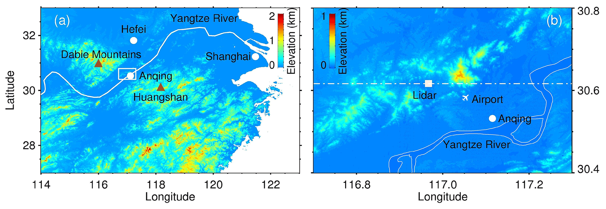
Figure 1(a) Terrain elevation map. (b) Enlarged area over Anqing station in the hollow white rectangle in (a). The computational domain is roughly along the white dash-dotted line in numerical simulations.
A field experiment is conducted to study the generation mechanism of GWs by the CDL at the National Meteorological Observing Station of Anqing (30∘37′ N, 116∘58′ E) from 16 August to 5 September 2018. Anqing is located near the Yangtze River and between Huangshan (30∘08′ N, 118∘10′ E) to the southeast and the Dabie Mountains (30–32∘ N, 115–117∘ E) to the northwest, as shown in Fig. 1a. The station is surrounded by hills with a relative elevation of 200–600 m, as shown in Fig. 1b. An airport is located to the southeast of the station.
2.1 Coherent Doppler wind lidar
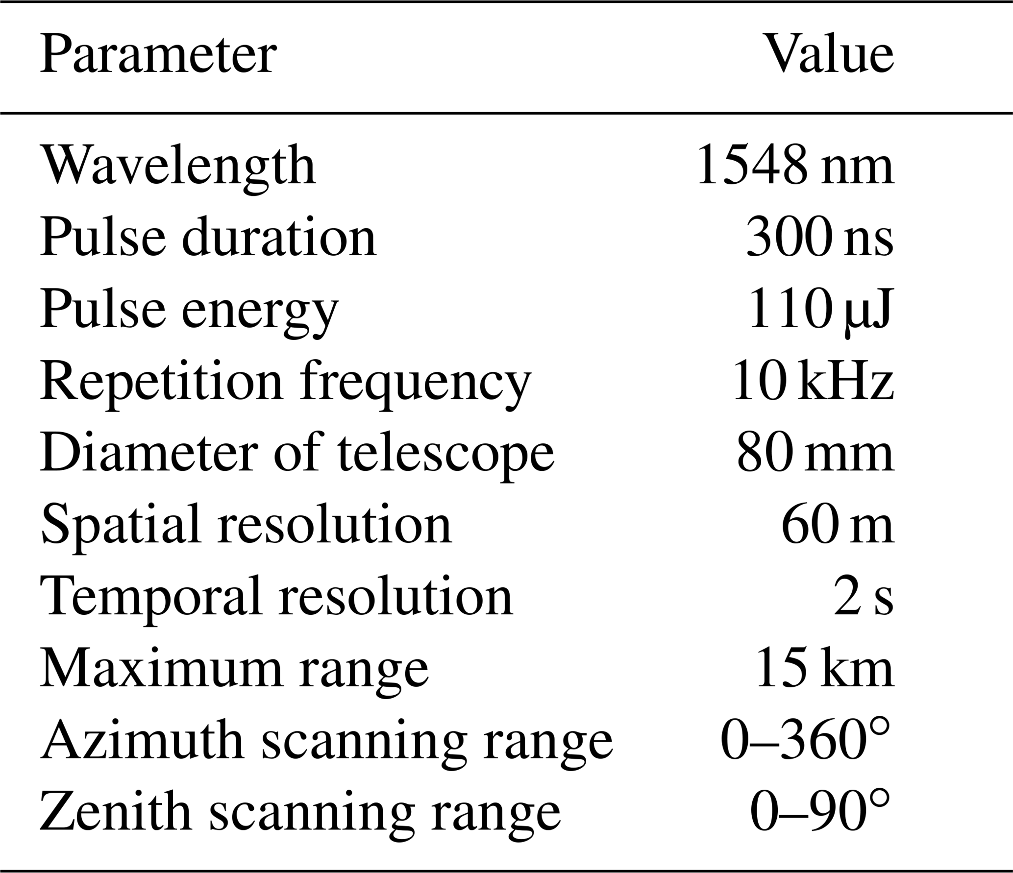
A compact micropulse CDL working at an eye-safe wavelength of 1.5 µm is used in this study. The pulse duration and pulse energy of the laser are 300 ns and 110 µJ, respectively. A double D-shaped telescope is employed. The absolute overlap distance and blind distance are ∼1 km and 60 m, respectively. This lidar has full hemispheric scanning capability with a rotatable transmitting and receiving system. Benefiting from coherent detection, this lidar can perform all-day measurement of radial wind speed based on the Doppler effect. Compared with traditional lidars, this CDL is small in size and robust in stability due to its all-fibre configuration. More details of this lidar are described in Wang et al. (2017). The key parameters of the CDL are listed in Table 1.
The wind field is composited by pointing the rotatable scanner in three directions during the experiment. First, the laser beam is pointed at two orthogonal azimuths sequentially, north and west, with a zenith angle of 30∘. Then, the laser beam is pointed vertically upward. In each direction, the measurement duration is set to 10 s. The full period of the measurement cycle is 41 s. The observational results, such as the vertical and horizontal wind components and the carrier-to-noise ratio (CNR) in the vertical beam, are shown in Appendix A. The blank areas without measurements are caused by rainy summers. For example, Tropical Storm Rumbia passed by around 17 August 2018. To guarantee the precision of the wind measurements, the data with a CNR of less than −35 dB are excluded (Wang et al., 2017, 2019).
2.2 Radiosonde
The National Meteorological Observing Station of Anqing is one of 120 operational radiosonde stations in mainland China (excluding Hong Kong; Li, 2006). The China Meteorological Administration has deployed an L-band (1675 MHz) sounding system at this station. Air temperature, pressure, relative humidity and wind from the ground to middle stratosphere can be measured twice a day at 07:15 and 19:15 by this sounding system, which combines a digital radiosonde with a secondary wind-finding radar. Previous studies have confirmed the accuracy measured by this type of radiosonde (Bian et al., 2010). A comparison between the wind measurements taken by the CDL and the radiosonde was carried out recently by Wei et al. (2019) to validate the performance of the CDL.
2.3 ERA5 reanalysis data
ERA5 is the fifth generation of the European Centre for Medium-Range Weather Forecasts (ECMWF) atmospheric reanalysis of the global climate. The ERA5 reanalysis assimilates a variety of observations and models in 4 dimensions. The data resolve the atmosphere with a horizontal resolution of 0.3∘ both longitudinally and latitudinally and using 137 levels from the surface up to an 80 km altitude (Hersbach and Dee, 2016). The hourly temperature data from the subdaily high-resolution-realization deterministic forecasts of ERA5 are used to calculate buoyancy frequency near the station in a later analysis in this study.
3.1 The long-lived GWs
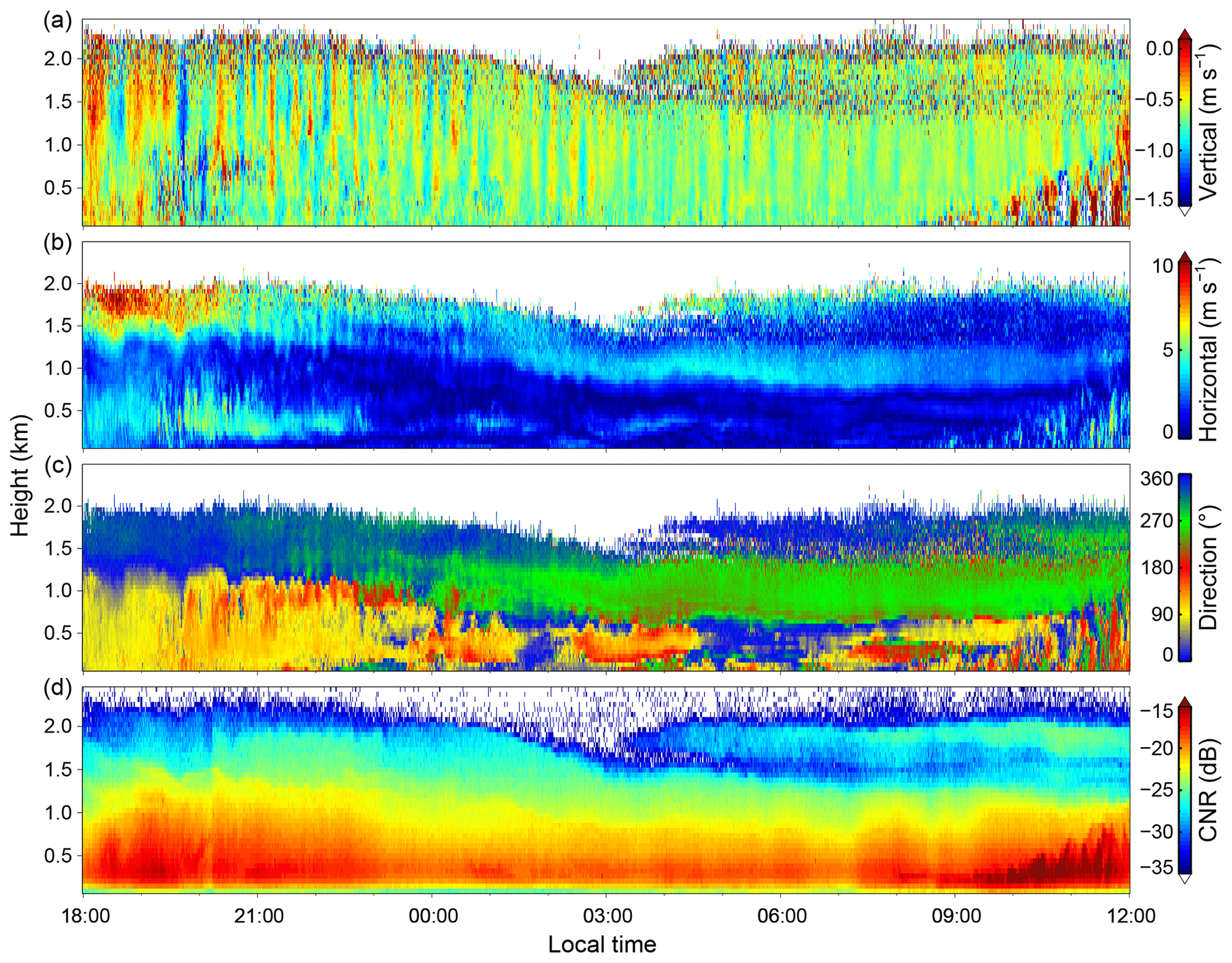
Figure 2Height–time cross sections of the (a) vertical wind speed, (b) horizontal wind speed, (c) horizontal wind direction and (d) CNR from the vertical beam obtained by the CDL from 4 to 5 September 2018. The direction is defined as the angle clockwise from north.
Figure 2a shows the persistent wave motions in the vertical wind lasting longer than 10 h in the ABL between 4 and 5 September 2018. These waves exist for longer than 20 periods and then dissipate during the evolution of the convective ABL on the morning of 5 September 2018. The corresponding horizontal wind speed and wind direction are shown in Fig. 2b and c, respectively. Two weak low-level jets are observed at heights of approximately 0.5 and 1.5 km. The lower easterly jet stream lasts only a few hours with a speed of approximately 5 m s−1, while the higher jet stream exists during the whole lifetime of the wave motion. The speed of the higher jet stream is approximately 10 m s−1 and then decreases to approximately 3–5 m s−1 after 21:00. The corresponding direction of this northerly jet stream also changes to westerly. The CNR from the vertical beam is shown in Fig. 2d; it varies slowly with time and is nearly stratified with altitude. Thus, the ABL seems to be stably stratified because the CNR may represent the aerosol concentration in some cases.

Figure 3(a) Mean vertical wind between 600 and 1000 m. (b) Corresponding wavelet power spectrum of the vertical wind in (a). The brown contours indicate a significance level of 95 %. The black solid lines represent the cone of influence.
The periods of these wave motions are typically approximately 10–30 min. The temporal profiles of the average vertical wind between 600 and 1000 m are plotted in Fig. 3a. Oscillations in the vertical wind can be seen clearly. The amplitudes of these wave motions are approximately 0.2 m s−1 before 03:00 and then decrease to approximately 0.15 m s−1, while the periods increased after 04:00. The wavelet power spectrum of the vertical wind in Fig. 3a is shown in Fig. 3b by using the Morlet mother wavelet. There are obvious waves with periods of 15–25 min before 03:00 and waves with periods of 20–30 min after ∼04:30. Relatively weak waves with periods of approximately 10 min are also observed between 03:00 and 05:00. These wave motions could be regarded as quasi-monochromatic waves as the periods vary within the range of 15–30 min. The change in periods may be in relation to changes in the background ABL, such as changes in the height of the upper jet stream.
Zonal wind can be derived from the horizontal wind speed and direction. The height-averaged perturbations in the vertical wind w′ and zonal wind u′ between 600 and 1000 m are shown in Fig. 4. First, the raw vertical (or zonal) winds are averaged between 600 and 1000 m. Second, the temporal profile of the averaged vertical (or zonal) winds is smoothed by a 1 h window as the background. Third, the background is subtracted to remove the trend. Finally, the perturbation is smoothed by averaging the adjacent three points to reduce high-frequency noises. It is obvious that wave motions also exist in the horizontal wind. The periods of zonal perturbations are similar to those of vertical perturbations. Specifically, the vertical and zonal perturbations are 90∘ out of phase, with the vertical perturbations w′ generally leading to zonal perturbations u′, especially after 02:00. Note that the wave motions exhibit highly coherent vertical motions with no apparent phase progression with altitude, as shown in Fig. 2a. These characteristics of wave motions indicate ducted wave structures within the ABL (Fritts et al., 2003).
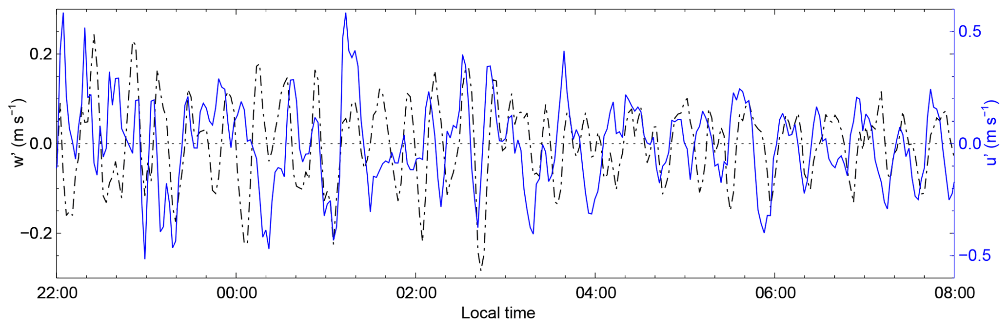
Figure 4Perturbations of vertical wind w′ (black dash-dotted line, left axis) and zonal wind u′ (blue solid line, right axis) obtained between 600 and 1000 m altitude from 22:00 on 4 September to 08:00 on 5 September 2018.
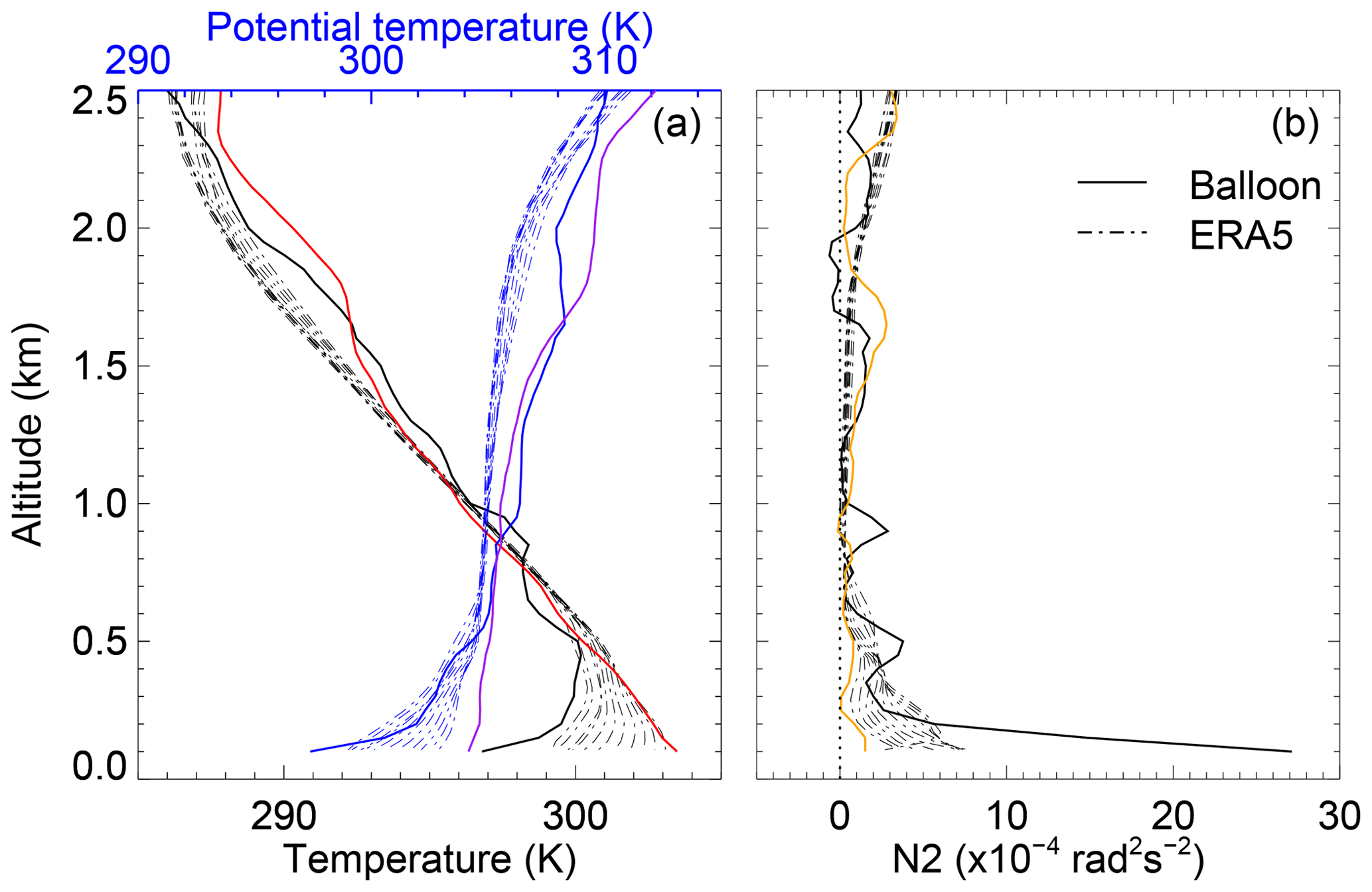
Figure 5(a) Temperature (black solid line) and potential temperature (blue solid line) profiles from radiosonde at 07:15 on 5 September and ERA5 (dash-dotted lines) between 22:00 on 4 September and 08:00 on 5 September. Profiles of temperature (red solid line) and potential temperature (purple solid line) from the radiosonde at 19:15 on 4 September are also plotted. (b) Corresponding buoyancy frequency profiles from radiosonde (black solid line) at 07:15 on 5 September and ERA5 (dash-dotted lines) between 22:00 on 4 September and 08:00 on 5 September. The buoyancy frequency profile (orange solid line) from the radiosonde at 19:15 on 4 September is also plotted.
Temperature profiles measured by the radiosonde attached to a weather balloon and hourly temperature profiles from ERA5 during the wave motions are shown in Fig. 5a. An inversion layer is observed below an altitude of ∼500 m. The corresponding squares of the buoyancy frequency,
are plotted in Fig. 5b, where g is the gravitational acceleration and θ is the potential temperature at altitude z. Maxima values of N2 larger than rad2 s−2 appear in the inversion layer from both the radiosonde and ERA5 data, indicating a strongly stratified stable boundary layer near the ground. Between ∼600 and ∼2000 m altitude, the values of N2 are so small that they are close to 0 and even negative at 1800–2000 m via the radiosonde. These results suggest thermal ducting between the ground and approximately ∼2000 m, in which the wave motions are trapped, especially under the inversion. This is why such wave motions have a lifetime longer than 20 periods. The buoyancy periods from Fig. 5b are typically 2–10 min. Since the background wind speeds are relatively small, less than ∼10 m s−1, we neglect the Doppler effects here. These wave motions should be GWs instead of internal acoustic waves. Therefore, these waves are suggested to be ducted gravity waves trapped in the ABL.
3.2 Background wind
There are complex relationships between GWs and background wind conditions. Submesoscale wavelike motions, which are defined as any nonturbulent motion at a horizontal scale smaller than 2 km and with a period at the scale of tens of minutes, are primarily generated under very weak winds in the nocturnal boundary layer (Mahrt, 2014). Note that the wind speed from 4 to 5 September 2018 is weakest during the whole field experiment, as shown in Fig. A2. To understand the relationship between this ducted GW and the background wind, a spatiotemporal window of 1 h length and 200 m height and temporal and vertical spatial step shifts of 1 h and 100 m, respectively, are used. The mean horizontal wind speed and wind direction in each window during the whole field campaign in Anqing are easily obtained.
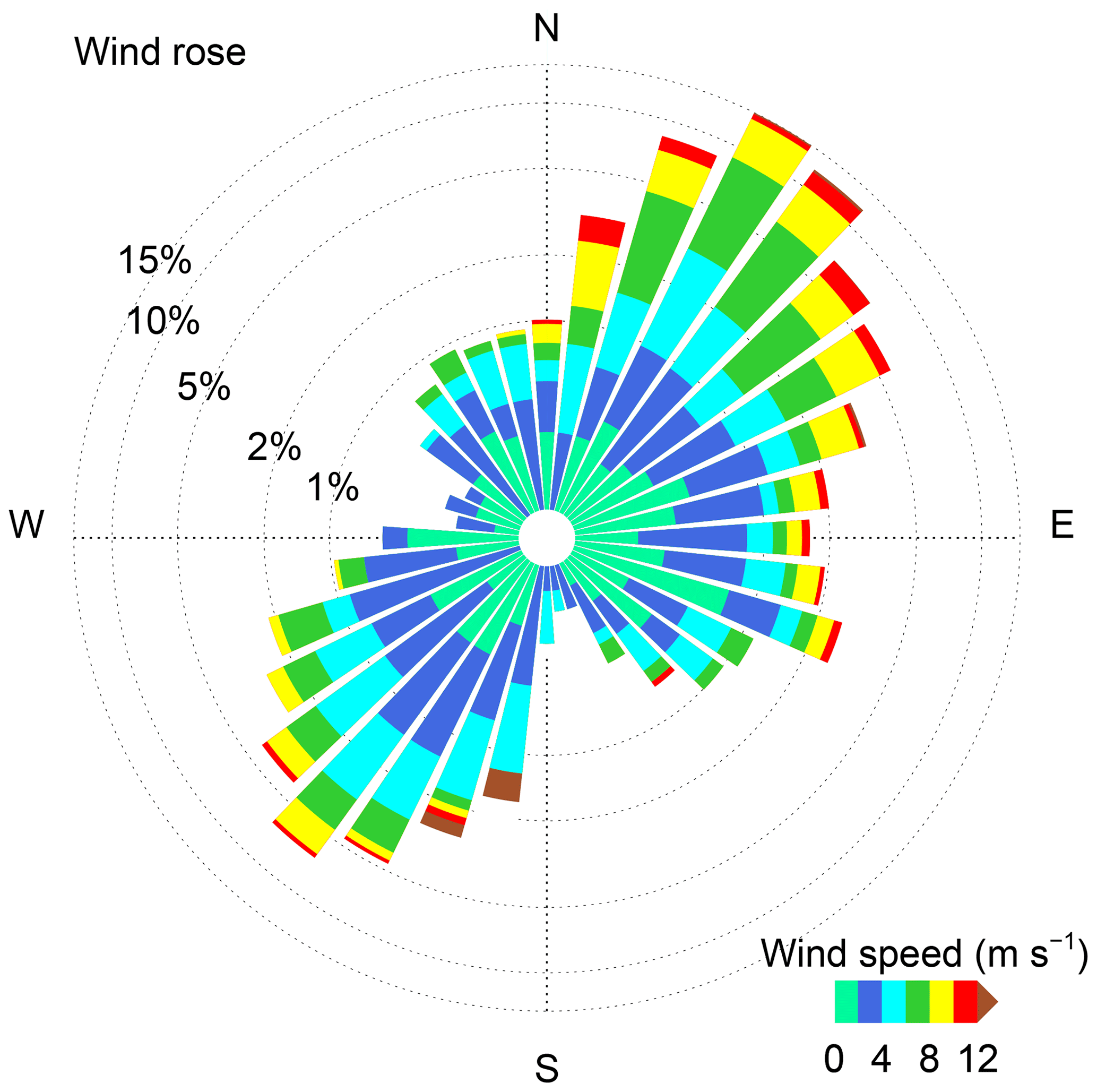
Figure 6Wind rose of horizontal wind in all temporal–spatial windows during this experiment. It should be noted that the value of the radius is logarithmic.
The wind rose of the horizontal wind during the field experiment is shown in Fig. 6. It is apparent that a northeasterly wind and southwesterly wind prevail around the station in the ABL during the whole field campaign. The infrequently observed ducted GWs in Fig. 2 accompany an infrequent westerly wind. It is interesting to note that the long, narrow plain area along the Yangtze River around Anqing between Huangshan and the Dabie Mountains is also along the northeast–southwest direction, as shown in Fig. 1a. The typical elevations of Huangshan and the Dabie Mountains are approximately 1–2 km. Strong winds along a northwest–southeast direction may be blocked in the ABL, thus leading to weak wind along the northwest–southeast direction after the wind flows over Huangshan or the Dabie Mountains and the prevailing wind flows along the northeast–southwest direction. As the GWs are favourable for generation under weak wind conditions, we can imagine that the Dabie Mountains and Huangshan may have an impact on GWs in Anqing. However, the surrounding hills around the station, as shown in Fig. 1b, may also affect the generation and existence of GWs. The effect of surrounding hills will be studied by numerical simulations in the next section.
Wavelike motions are common in the stably stratified ABL and may be generated by topography or the jet stream (Mahrt, 2014). There is a complex topography around the station, as shown in Fig. 1b, and a low-level jet in the ABL, as shown in Fig. 2. Both of these phenomena may be responsible for the generation of persistent GWs. To identify the potential source of the ducted GWs, a numerical simulation based on CFD is performed to simulate the fluid flow field. The impact of different boundary conditions, e.g. wind profile and topography, on atmospheric dynamics can be effectively evaluated by changing them. In addition, the numerical simulations can provide complete information on the GWs. This information, such as horizontal wavelength or horizontal phase speed, cannot be obtained by lidar in this experiment. Therefore, CFD simulations are helpful for investigating GWs in the ABL.
4.1 Model description
Reynolds-averaged Navier–Stokes (RANS) simulations have been widely used to investigate the wind field over the past few decades (Toparlar et al., 2017). Compared with a large eddy simulation (LES), a RANS simulation has the advantages of low computational cost and sufficient accuracy. In this study, a two-equation RANS model based on the renormalization group (RNG) method is used to simulate the wind field. The RNG k-ε model was developed to renormalize the Navier–Stokes equations, which account for the effects of small-scale motions (Yakhot et al., 1992). The RNG k-ε model is a mature model that has been widely verified in the simulation of wind flow over complex terrain in recent years (El Kasmi and Masson, 2010; Yan et al., 2015). The RNG k-ε turbulence model used in this work is based on OpenFOAM. OpenFOAM is the leading free, open-source software for CFD simulations. The model transport equations are obtained as follows:
where t and ρ are time and air density, respectively; k and ε are turbulence kinetic energy (TKE) and TKE dissipation rate, respectively; xi and xj are the displacement in dimensions i and j, respectively; ui is the velocity in dimension i; αk and αε are the inverse effective Prandtl numbers for k and ε, respectively; μeff is the effective viscosity; Gk and Gb represent the generation of TKE due to the mean velocity gradient and buoyancy, respectively; YM represents the contribution of the fluctuating dilatation in compressible turbulence to the overall dissipation rate; Sk and Sε are user-defined source terms; and G1ϵ, C2ϵ and C3ε are constants. In this paper, the input turbulent parameters recommended by OpenFOAM are applied. The default model coefficients of RNG k-ε are as follows: ; and αε=1.22.

Figure 7(a) The topography used in CFD simulations. A/B represents west/east hill. The heights of A and B are represented by hA and hB, respectively. (b) The vertical profile of potential temperature used in the CFD model. (c) The vertical profile of the inlet wind in the CFD model. (d) The vertical wind perturbation from lidar 00:00–09:00 on 5 September 2018. A mean value is subtracted. (e) The CFD-simulated results of vertical wind. (f) Observed (black) and simulated (red) vertical perturbations at 1 km altitude. The observed perturbation is smoothed with five-point smoothing.
To simplify the numerical simulation processes, a two-dimensional rectangular computational domain is applied in this study, with a horizontal range of 70 km and a 5 km range vertical from the sea level. The upper interface extended to 5 km is set as the symmetric condition to prevent the influence of the upper interface on the region below 2 km. Under this condition, a zero gradient is set for all vertical physical variables, and the vertical velocity is set to 0. The vertical height of the first layer of grid cells is 5 m. The spatial resolution is approximately 20 m in both the horizontal and vertical planes. The total number of computational grid cells is 875 000. The velocity inlet is westerly and constant in the western boundary of the computational domain. The easterly interface is set as a pressure-outlet boundary to improve reversed flow. The topography is set to have a no-slip wall condition. A rough wall function is adopted, of which the formula is as follows (Ren et al., 2018):
where E=9.793 is the wall constant, C=0.327 is a roughness constant, K≈0.4 is the von Kármán constant, ks is the roughness height, zc is the distance to the cell centre of the first adjacent wall cell, u is the velocity in the cell centre and u∗ is the friction velocity. The simulation is run with a time step of 0.5 s.
The CFD cases conducted in this study are used to reveal the influence of topography and wind shear on the generation of persistent GWs. The initial thermal field is assumed to be horizontally uniform, using the vertical temperature profile from the radiosonde on 5 September 2018. The topography is set at a fixed temperature, since the heat flux at the ground was unavailable. In this work, buoyant flows are developed with low velocity and small temperature variations in each layer. The Boussinesq approximation, which treats density ρref(z) as a constant value at altitude z in all solved equations, except for the gravity and buoyancy terms in the momentum equation, is applied for each thin layer. The fluctuation of ρ(z) is caused by temperature T(z), neglecting the influence of pressure. The density ρ(z) is approximated as follows:
where β is the thermal expansivity and Tref(z) is the reference temperature at altitude z. The Boussinesq approximation is similar to the anelastic approximation in this form. The main difference between the Boussinesq and anelastic approximations is that the latter considers the influence of both pressure and temperature in fluctuations of ρ. Considering computational convenience and convergence, the Boussinesq approximation is adopted in this work.
4.2 Numerical simulations
The initial smoothed topography is shown in Fig. 7a. The horizontal location of the domain is roughly along the zonal white dash-dotted line in Fig. 1b. This is because the low-level jet and the background wind are mainly in the zonal (east–west) direction. The influence of terrain on atmospheric flow is mainly in this direction. The left (west) hill is defined as A with a height of hA and the right (east) hill is defined as B with a height of hB in this study. The maximum elevation of A and B are approximately 250 and 600 m, respectively. The lidar is located between A and B. The 1 h mean zonal wind under 2 km from the lidar and the zonal wind above 2 km from the ERA5 reanalysis data at 00:00 on 5 September 2018 are merged into a sustained imported wind profile u0 along the western boundary of the computational domain. The vertical profiles of potential temperature and u0 used in the CFD models are shown in Fig. 7b and c, respectively. The measured vertical wind perturbation w′ with the mean value subtracted from it is shown in Fig. 7d. The vertical wind from the CFD simulations is shown in Fig. 7e. The measured and simulated vertical perturbations at 1.0 km are compared in Fig. 7f. It is obvious that a similar wave motion with a similar amplitude and period exists in the ABL. This result verifies the accuracy of the CFD numerical simulation results in this study. A short video of the zonal wind and vertical wind in the whole computational domain can be downloaded from the Supplement. From this video, the zonal wavelength can be estimated as ∼3 km and the corresponding zonal phase speed as ∼2 m s−1. In addition, Kelvin–Helmholtz billows exist in the low-level jet around an altitude of 2 km. These billows may be in relation to the GWs.
Based on this result, wind profiles uz with different wind shear and topography with different height of hills A and B are employed in the CFD numerical simulations. A detailed list of boundary conditions is presented in Table 2. The simulated zonal winds and vertical winds above the lidar for all cases are shown in Fig. 8. It should be noted that a time of 0 represents a steady state, not the real time after the simulations started running, in all cases except cases 7 and 8. Here, we mean by a steady state that which pertains when the turbulence is fully developed. In cases 7 and 8, a time of 0 is defined as that when the simulations started running and the input velocity flowed from the western boundary at the same time.
In case 1, persistent wave motions not only exist in the vertical wind but also in the zonal wind near and below the low-level jet at approximately 2 km, as shown in Fig. 8. This is consistent with lidar detections, as shown in Fig. 4. It is obvious that no wave motions are generated, with uniform wind speeds of 1, 5 and 10 m s−1 in cases 2–4, respectively. Thus, GWs cannot be excited without wind shear. From the results of cases 1, 5 and 6, the wave amplitudes and frequencies increase with enhancement in the wind shear. For cases 1, 7 and 8, no persistent wave motions exist with the increase in wind speed without enhancement in the wind shear. Only several solitary wavelike motions can be found when the wind flow passes by the lidar and dissipates rapidly. In addition, the wave motions in cases 1–8 mainly exist under 2.5 km, where the wind speeds are relatively weak. Therefore, it can be inferred that it is beneficial to the generation of persistent waves under persistent weak-wind conditions, which is consistent with the previous result in Sect. 3.2.
Table 2The wind profile and topography for each case in CFD simulations.
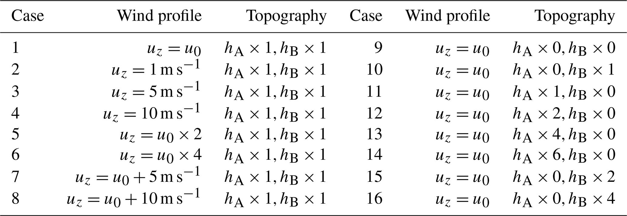
What happens when the heights of hills A and B near the lidar location change? In cases 9–11, persistent wave structures still exist with only a few changes when hills A and/or B disappear. From cases 9 and 11–13, persistent wave structures always exist and do not change significantly. When the height of hill A increases to hA×6 in case 14, i.e. the height of the low-level jet near a 2 km altitude, the zonal wind structure changes significantly. In cases 9–10 and 15–16, wave motions also exist and do not change significantly even though the height of hill B increases to the height of the low-level jet, hB×4.
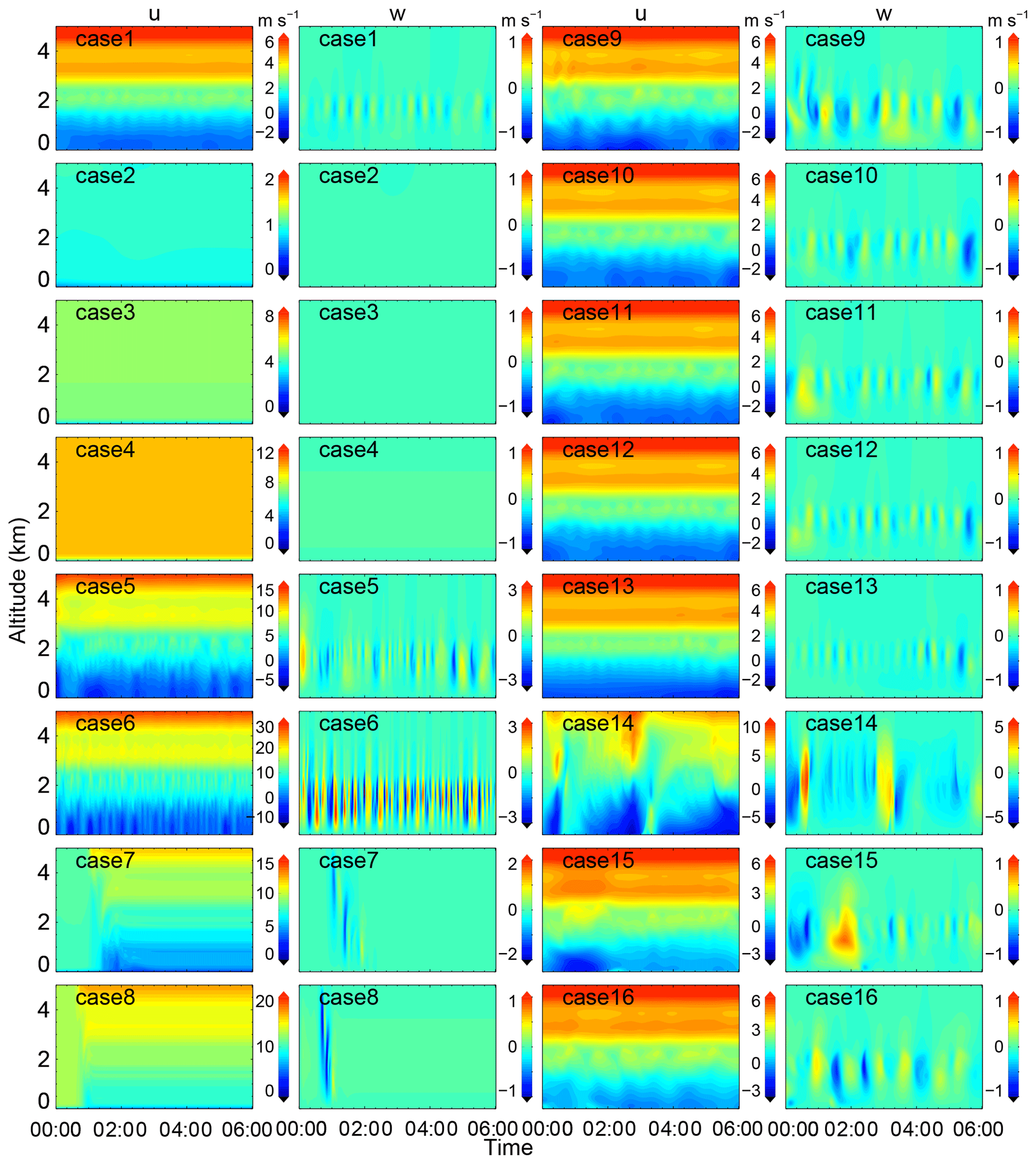
Figure 8The simulated zonal wind u and vertical wind w above the lidar for all 16 cases as described in Table 2.
Therefore, based on these results from the simulation cases, persistent GWs are excited by persistent wind shear around the low-level jet. The wave structures mainly occur under weak winds. The topography, i.e. the hills near the station, as shown in Fig. 1b, plays a negligible role in GW generation. Nevertheless, the topography may play a more important role downstream where the height of the jet is comparable with the height of the terrain.
Based on the above experiments and simulations, the mechanism of the persistent wave motions can be inferred as follows: a westerly low-level jet of ∼5 m s−1 exists above the light southeasterly background wind. The light wind may be understood in relation to Huangshan and the Dabie Mountains. The weak wind shear around the low-level jet may lead to the occurrence of wave motions in the light wind. In addition, a strongly stable thermally stratified ABL with an inversion layer occurs during the night in Anqing. Negative values of N2 appear near an altitude of ∼2 km. Therefore, the wave motions may be trapped in a ducted structure with a long lifetime. The GWs exist without apparent phase progression with altitude in the whole ABL from the surface to a height of ∼2 km.
Such quasi-monochromatic waves with multiple wave cycles and approximately constant periods and amplitudes are infrequently observed in the ABL (Mahrt, 2014). Nevertheless, similar quasi-monochromatic wave motions with multiple wave cycles have been reported in several studies. Banakh and Smalikho (2016) revealed a coastal mountain lee wave with a period of ∼9 min during the daytime on 23 August 2015 in the stably stratified ABL over the shore of Lake Baikal. The wave existed between the 100 and 900 m height range with a lifetime of approximately 4 h. This wave was suggested to be in relation to the presence of two narrow jet streams at heights of approximately 200 and 700 m above ground level. Similar wave motions were also detected in the vertical wind accompanied with a low-level jet in Banakh and Smalikho (2018). It is regrettable that the authors did not give a discussion on the contaminated wavelike motions from 01:00 to 08:00, except with regard to the internal wave with a period of ∼6 min at 07:00. Fritts et al. (2003) reported wave motions with typical periods of 4–5 min below a height of ∼800 m under light wind with low-level jet and clear-sky conditions throughout the night of 14 October 1999. These wave motions were interpreted as ducted GWs that propagated horizontally along the maxima of the stratification and mean wind and were evanescent above and possibly below and/or between the ducting level(s) (Fritts et al., 2003). Viana et al. (2009) also reported a ducted mesoscale gravity wave over a weakly stratified nocturnal ABL. This wave lasted less than 10 wave cycles, approximately 2 h, with a period of ∼16 min. Román-Cascón et al. (2015) analysed nonlocal GWs generated by wind shear or the low-level jet trapped within the stable ABL. With an acoustic echo sounder, similar wave motions were also observed without apparent phase progression with altitude in a stably stratified ABL several decades ago (Beran et al., 1973; Hooke and Jones, 1986).
The wave motions mentioned above were mainly observed in the stable boundary layer under a height of ∼1000 m or even ∼100 m, while wave motions exist from the surface layer to as high as ∼2000 m in our study due to different measurement capabilities. In addition, the lifetime of the ducted GWs is more than 10 h and 20 wave cycles, while in the previous studies listed above most of the lifetimes are shorter in duration with several wave cycles. These characteristics make these ducted GWs unique and novel. However, in one of our previous studies, obvious wave motions with periods of 10–30 min in the vertical wind were observed in the whole residual layer from 1 to 2 June 2018 by a similar CDL system (Wang et al., 2019).
The mechanism of these long-lived GWs is consistent with that of other similar wave motions referenced above in some aspects. The low-level jet or wind shear is one of the main sources of such wavelike motions in the ABL. A stably stratified ABL usually leads to effective quasi-monochromatic ducted wave motions with a long lifetime and multiple wave cycles. Although wind shear near the low-level jet is the main source of GWs as discussed in Sect. 4.2, weaker wind shear is more favourable to the existence of high-frequency GWs. Similarly, the surrounding hills play a negligible role in generating the ducted GWs while the Dabie Mountains and Huangshan may have an impact on the generation and existence of GWs.
The vertical structure of GWs is described by the Taylor–Goldstein equation (Gossard and Hooke, 1975):
where m is the vertical wavenumber, ci is the intrinsic phase speed in the direction of propagation, is the second derivative with the height of the mean wind in the direction of wave propagation, kh is the horizontal wavenumber, and H is the scale height. A sufficiently deep atmospheric layer is required for a wave duct with positive values of m2. To resolve this equation, the vertical profile of squared buoyancy frequency, which is calculated by the temperature profile measured by the radiosonde, is shown in Fig. 5b. Simultaneous hourly mean wind, which is required to resolve ci and , can be obtained from the lidar measurements. However, the horizontal structures of this wave motion, i.e. ci and kh, are still unclear in this study. The horizontal structures of wavelike motions in the ABL can be detected by airborne lidar (Chouza et al., 2016; Witschas et al., 2017) and ground-based lidar with range–height indicator (RHI) scans (Poulos et al., 2002; Wang, 2013) or plan position indicator (PPI) scans (Mayor, 2017). GW parameters, such as horizontal phase speed, horizontal wavelength, propagation direction, and intrinsic frequency, can be resolved from these measurements. Nevertheless, we try to illustrate the characteristics of this ducted wave to determine a plausible propagation direction and horizontal wavelength in accordance with the CFD simulations. The propagation direction is assumed to be westerly here, as the simulated wave is westerly according to the video available in the Supplement. Thus, the horizontal wavelength is equal to the zonal wavelength, which is estimated as ∼3 km in Sect. 4.2.
The vertical profile of the vertical wave number squared is shown in Fig. 9. The singular point of the relative maxima m2 towards the right-hand side of the figure is caused by a critical level where the intrinsic frequency is Doppler-shifted close to 0. A ducting process occurs between ∼1.5 km altitude and the ground where m2>0. This is the result of a combination of thermal and Doppler ducts. The thermal duct is dominant under the temperature inversion with a maximum buoyancy frequency squared for all propagation directions, as shown in Fig. 5. The Doppler duct is dominant between the ∼0.5 and ∼1.5 km altitude range due to the critical level induced by the low-level jet of wind maximum in a particular direction. Thus, the ducted motions give a plausible explanation for the long-lived trapped GWs in the ABL.
Figure 9The vertical profile of the vertical wave number squared. The dotted line represents the zero line.
It should be noted that the retrieval of horizontal wind is based on the hypothesis of a homogeneous wind field on a horizontal plane. Accompanying the wave activities, the radius of the scanning beam cone leads to a bias in the retrieved horizontal wind. If the radius is equivalent to or larger than the scale of the horizontal wavelength of the GWs, these biases may significantly affect the result in the horizontal plane, especially the amplitude of the retrieved GWs. Nevertheless, the bias in the period of the wave motion is negligible. If the radius is smaller than the scale of the horizontal wavelength of the GWs, the biases in both amplitude and period can be ignored. In this study, the horizontal wavelength is estimated to be ∼3 km in Sect. 4.2. The radii are approximately 580 m and 870 m at 1 km and 2 km altitude, respectively. Thus, the retrieved bias can be ignored in this study.
A 2-D model is used in this simulation rather than a 3-D model which in principle can more accurately simulate the atmospheric flow. Considering the direction of the low-level jet and the maximum background wind flow, the zonal transect in this case is appropriate for a 2-D model; the influence of terrain on atmospheric flow is mainly in this direction. However, the 2-D model cannot simulate the information in another dimension, e.g. lateral flow around the hillside and the blocking effect of the low terrain on both sides, leading to errors compared with a 3-D model. Nevertheless, comparison between numerical simulation results and field experiments show that 2-D models can simulate the actual topographic flow well in some cases (Miller and Davenport, 1998; Toparlar et al., 2017; Walmsley et al., 1984). Furthermore, some basic theories and empirical formulas of complex mountain wind fields are built on the basis of a 2-D model. In addition, a 2-D model consumes many fewer computing resources and much less time than 3-D models. Therefore, the 2-D terrain simulation of the mountain wind field has wide-ranging theoretical significance and applicability. By using this simplified 2-D model, the influence of terrain on GWs can be analysed.
A persistent wave motion was investigated by experiments and numerical simulations. From 4 to 5 September 2018, GWs with periods of 10–30 min were observed in the whole ABL from the ground to a height of ∼2 km by a coherent Doppler lidar during a field experiment in Anqing. The amplitudes of these GWs were approximately 0.15–0.2 m s−1 in the vertical wind direction. These GWs existed for longer than 20 wave cycles. The periods were approximately 15–25 min before 03:00 and 20–30 min after 03:00. A westerly low-level jet was observed at an altitude of 1–2 km in the ABL with maxima speeds of 5–10 m s−1. Simultaneous temperature profiles from radiosonde measurements and ERA5 reanalysis data confirmed the existence of a strong stably stratified ABL. There was an inversion layer below the altitude of ∼500 m and a negative buoyancy frequency squared near the height of ∼2 km. Note that there was no apparent phase progression with altitude for these GWs. Moreover, the vertical and zonal perturbations in the GWs were 90∘ out of phase with the vertical perturbations generally leading zonal perturbations. These characteristics suggested that such GW motions are ducted GWs trapped in the ABL, which is also verified by the vertical structure of the wave motions. Based on simplified 2-D CFD numerical simulations, the generation mechanisms of such GWs were discussed. The low-level jet streams were considered to be responsible for the excitation of GW motion in the present study. Wave motions mainly occurred under weaker wind conditions, which was consistent with other studies of ducted waves. The contributions from wind flow over the surrounding hills could be ignored.
The current study contributes to our understanding of the GW generation mechanism in the ABL, which plays a key role in atmospheric dynamics. Furthermore, the National Meteorological Observing Station of Anqing is close to an airport, as shown in Fig. 1b, which will be affected by clear-air turbulence caused by breaking GWs and rotors affected by the trapped GWs. The application of such a coherent Doppler lidar will enhance measurement capability generating high-quality data in the ABL, thus enriching our knowledge and improving aviation safety, weather forecasting and climate modelling in the future. However, the horizontal structures of GWs are still unclear in this study. Simultaneous measurements with multiple lidars and multiple scanning modes are required in additional studies.
The ERA5 data sets are publicly available from the ECMWF website at https://cds.climate.copernicus.eu/cdsapp#!/home (last access: 1 March 2019; C3S, 2017). The elevation data are available on the Shuttle Radar Topography Mission (SRTM) website at http://srtm.csi.cgiar.org (last access: 1 March 2019; Jarvis et al., 2008). Lidar and radiosonde data can be downloaded from http://www.lidar.cn/datashare/Jia_et_al_2019.rar (last access: 16 March 2019; Jia et al., 2019).
A video of vertical wind and horizontal wind simulated by a CFD model in the whole 2-D computational domain for case 1 in Table 2 is provided (https://doi.org/10.5446/41847, Jia and Yuan, 2019).
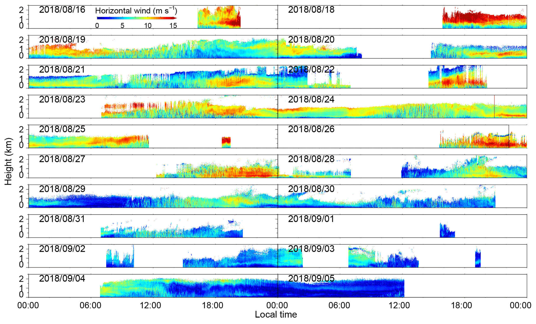
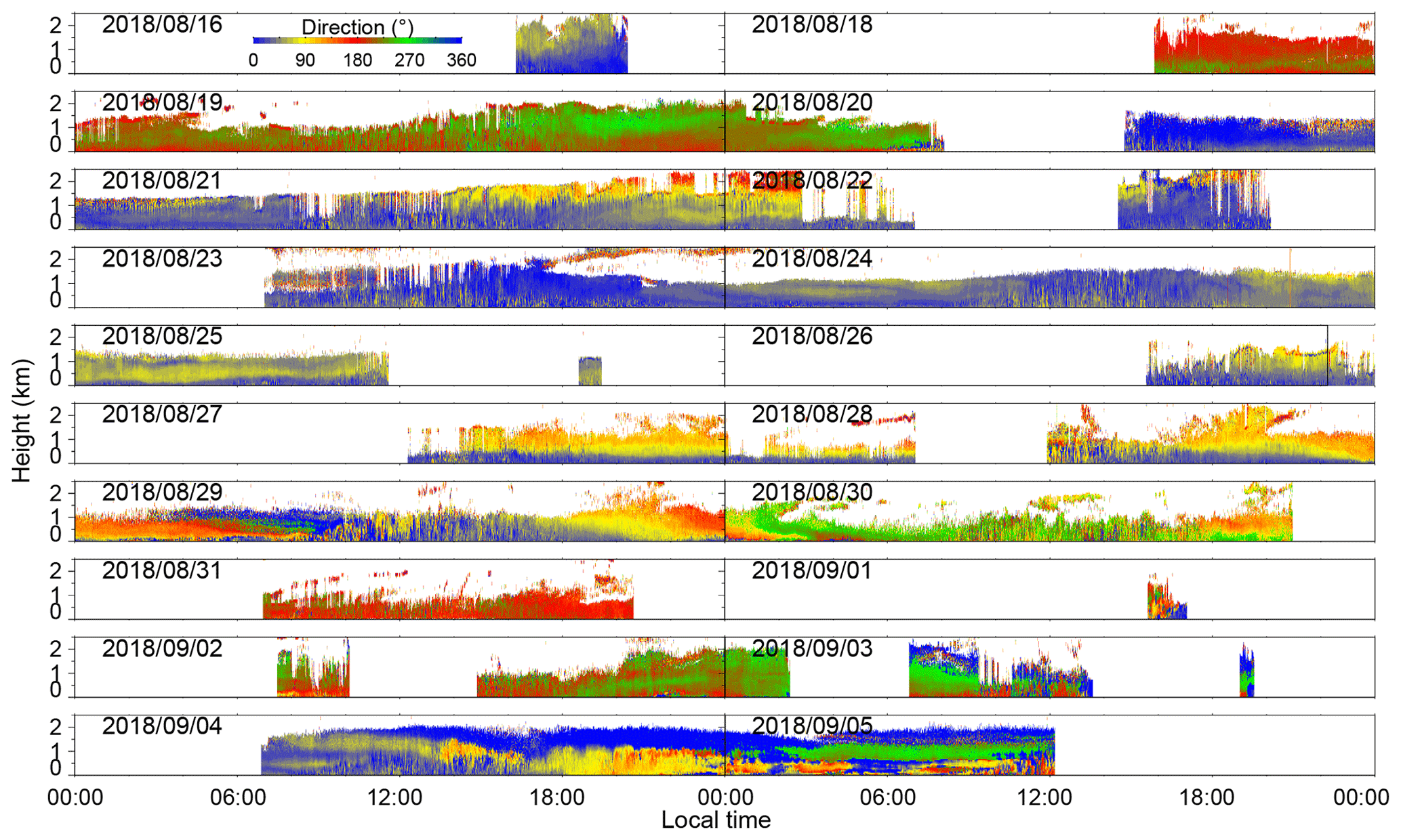
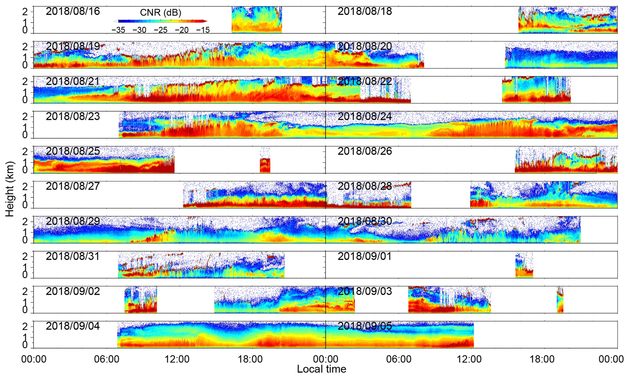
The vertical wind, horizontal wind speed, wind direction and CNR during the field experiment from 16 August to 5 September 2018 are shown in Figs. A1–A4, respectively.
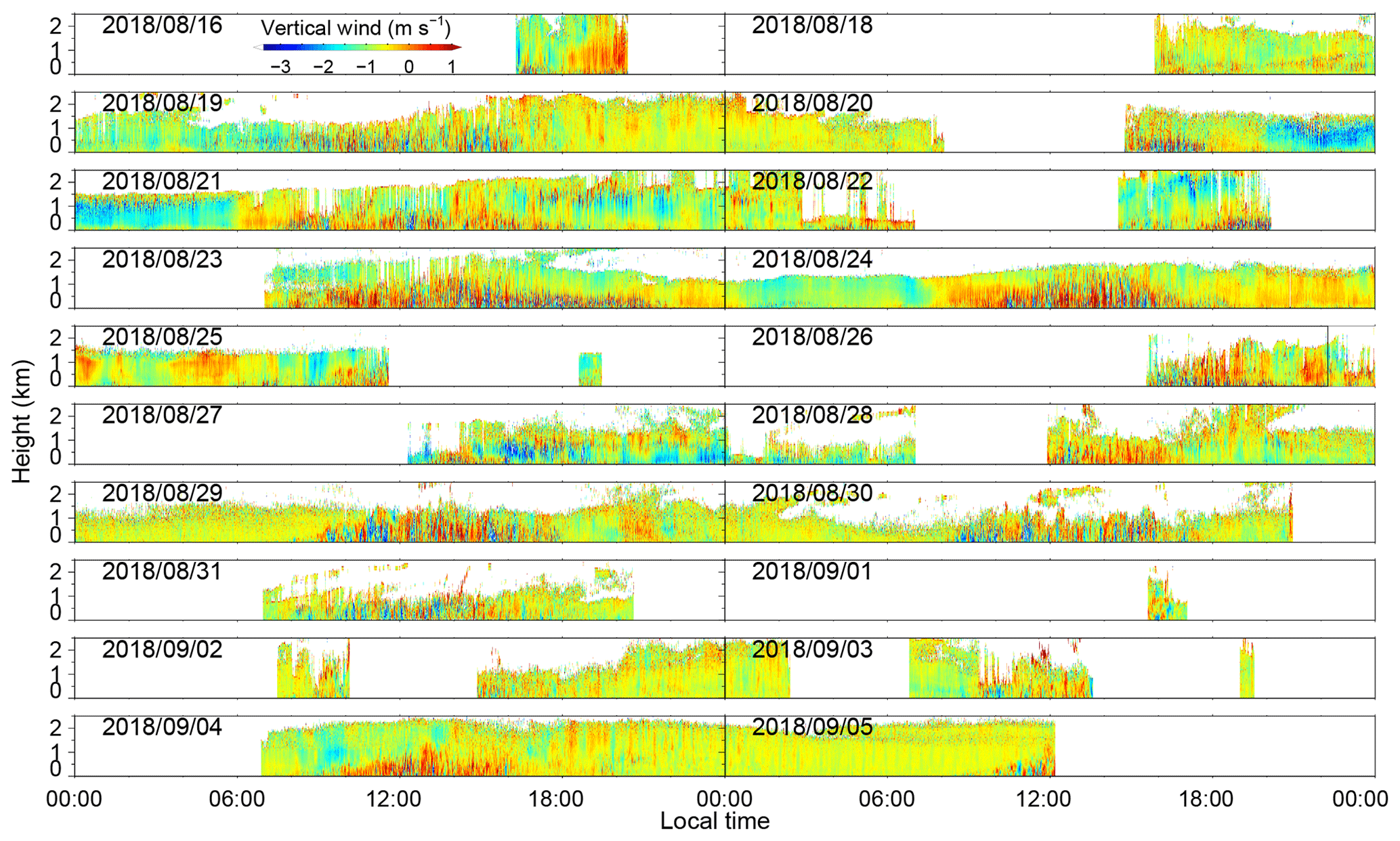
Figure A1Time–height cross section of vertical wind speed per day during the experiment. Dates are shown in the top left of each panel, and are read as YYYY/MM/DD.
HX conceived of and designed the study. YW, LZ CW and MJ performed the lidar experiments. MJ, CW and TW performed the lidar data analysis. LL, DL and RC provided the field experiment site and the radiosonde data. JW analysed ERA5 data. JY performed the CFD numerical simulations. MJ and JY carried out the analysis and prepared the figures with comments from the other coauthors. MJ, HX, XX and XD interpreted the data. MJ, JY and HX wrote the manuscript. All authors read and approved the final manuscript.
The authors declare that they have no conflict of interest.
We acknowledge the use of ERA5 data sets from the ECMWF website at https://www.ecmwf.int/en/forecasts/datasets/ reanalysis-datasets/era5 (last access: 1 March 2019). We acknowledge the use of elevation data sets from the SRTM website at http://srtm.csi.cgiar.org (last access: 1 March 2019).
This paper was edited by Geraint Vaughan and reviewed by two anonymous referees.
Banakh, V. and Smalikho, I.: Lidar Studies of Wind Turbulence in the Stable Atmospheric Boundary Layer, Remote Sens., 10, 1219, https://doi.org/10.3390/rs10081219, 2018.
Banakh, V. A. and Smalikho, I. N.: Lidar observations of atmospheric internal waves in the boundary layer of the atmosphere on the coast of Lake Baikal, Atmos. Meas. Tech., 9, 5239–5248, https://doi.org/10.5194/amt-9-5239-2016, 2016.
Beran, D. W., Hooke, W. H., and Clifford, S. F.: Acoustic echo-sounding techniques and their application to gravity-wave, turbulence, and stability studies, Bound.-Lay. Meteorol., 4, 133–153, https://doi.org/10.1007/bf02265228, 1973.
Berg, J., Troldborg, N., Sørensen, N. N., Patton, E. G., and Sullivan, P. P.: Large-Eddy Simulation of turbine wake in complex terrain, J. Phys.: Conference Series, 854, 012003, https://doi.org/10.1088/1742-6596/854/1/012003, 2017.
Bian, J., Chen, H., Vömel, H., Duan, Y., Xuan, Y., and Lü, D.: Intercomparison of humidity and temperature sensors: GTS1, Vaisala RS80, and CFH, Adv. Atmos. Sci., 28, 139-146, https://doi.org/10.1007/s00376-010-9170-8, 2010.
Birch, C. E., Parker, D. J., O'Leary, A., Marsham, J. H., Taylor, C. M., Harris, P. P., and Lister, G. M. S.: Impact of soil moisture and convectively generated waves on the initiation of a West African mesoscale convective system, Q. J. Roy. Meteorol. Soc., 139, 1712–1730, https://doi.org/10.1002/qj.2062, 2013.
Blumen, W., Banta, R. M., Berri, G., Blumen, W., Carruthers, D. J., Dalu, G. A., Durran, D. R., Egger, J., Garratt, J. R., Hanna, S. R., Hunt, J. C. R., Meroney, R. N., Miller, W., Neff, W. D., Nicolini, M., Paegle, J., Pielke, R. A., Smith, R. B., Strimaitis, D. G., Vukicevic, T., and Whiteman, C. D.: Atmospheric Processes over Complex Terrain, Meteorological Monographs, 57, Am. Meteorol. Soc., Boston, MA, 1990.
C3S (Copernicus Climate Change Service): ERA5: Fifth generation of ECMWF atmospheric reanalyses of the global climate. Copernicus Climate Change Service Climate Data Store (CDS), available at: https://cds.climate.copernicus.eu/cdsapp#!/home (last access: 4 December 2019), 2017.
Chouza, F., Reitebuch, O., Jähn, M., Rahm, S., and Weinzierl, B.: Vertical wind retrieved by airborne lidar and analysis of island induced gravity waves in combination with numerical models and in situ particle measurements, Atmos. Chem. Phys., 16, 4675–4692, https://doi.org/10.5194/acp-16-4675-2016, 2016.
Clark, T. L., Hall, W. D., Kerr, R. M., Middleton, D., Radke, L., Ralph, F. M., Neiman, P. J., and Levinson, D.: Origins of aircraft-damaging clear-air turbulence during the 9 December 1992 Colorado downslope windstorm: Numerical simulations and comparison with observations, J. Atmos. Sci., 57, 1105–1131, https://doi.org/10.1175/1520-0469(2000)057<1105:Ooadca>2.0.Co;2, 2000.
Cohn, S. A., Holloway, C. L., Oncley, S. P., Doviak, R. J., and Lataitis, R. J.: Validation of a UHF spaced antenna wind profiler for high-resolution boundary layer observations, Radio Sci., 32, 1279–1296, https://doi.org/10.1029/97rs00578, 1997.
Cohn, S. A., Brown, W. O. J., Martin, C. L., Susedik, M. E., Maclean, G. D., and Parsons, D. B.: Clear air boundary layer spaced antenna wind measurement with the Multiple Antenna Profiler (MAPR), Ann. Geophys., 19, 845–854, https://doi.org/10.5194/angeo-19-845-2001, 2001.
Corby, G. A.: A preliminary study of atmospheric waves using radiosonde data, Q. J. Roy. Meteorol. Soc., 83, 49–60, https://doi.org/10.1002/qj.49708335505, 1957.
Einaudi, F. and Finnigan, J. J.: The interaction between an internal gravity wave and the planetary boundary layer. Part I: The linear analysis, Q. J. Roy. Meteorol. Soc., 107, 793–806, https://doi.org/10.1002/qj.49710745404, 1981.
El Kasmi, A. and Masson, C.: Turbulence modeling of atmospheric boundary layer flow over complex terrain: a comparison of models at wind tunnel and full scale, Wind Ener., 13, 689–704, https://doi.org/10.1002/we.390, 2010.
Fernando, H. J. S., Mann, J., Palma, J. M. L. M., Lundquist, J. K., Barthelmie, R. J., BeloPereira, M., Brown, W. O. J., Chow, F. K., Gerz, T., Hocut, C. M., Klein, P. M., Leo, L. S., Matos, J. C., Oncley, S. P., Pryor, S. C., Bariteau, L., Bell, T. M., Bodini, N., Carney, M. B., Courtney, M. S., Creegan, E. D., Dimitrova, R., Gomes, S., Hagen, M., Hyde, J. O., Kigle, S., Krishnamurthy, R., Lopes, J. C., Mazzaro, L., Neher, J. M. T., Menke, R., Murphy, P., Oswald, L., Otarola-Bustos, S., Pattantyus, A. K., Rodrigues, C. V., Schady, A., Sirin, N., Spuler, S., Svensson, E., Tomaszewski, J., Turner, D. D., van Veen, L., Vasiljević, N., Vassallo, D., Voss, S., Wildmann, N., and Wang, Y.: The Perdigão: Peering into Microscale Details of Mountain Winds, B. Am. Meteorol. Soc., 100, 799–819, https://doi.org/10.1175/bams-d-17-0227.1, 2018.
Finnigan, J. J. and Einaudi, F.: The interaction between an internal gravity wave and the planetary boundary layer. Part II: Effect of the wave on the turbulence structure, Q. J. Roy. Meteorol. Soc., 107, 807–832, https://doi.org/10.1002/qj.49710745405, 1981.
Fritts, D. C. and Alexander, M. J.: Gravity wave dynamics and effects in the middle atmosphere, Rev. Geophys., 41, 64, https://doi.org/10.1029/2001rg000106, 2003.
Fritts, D. C., Nappo, C., Riggin, D. M., Balsley, B. B., Eichinger, W. E., and Newsom, R. K.: Analysis of Ducted Motions in the Stable Nocturnal Boundary Layer during CASES-99, J. Atmos. Sci., 60, 2450–2472, https://doi.org/10.1175/1520-0469(2003)060<2450:aodmit>2.0.co;2, 2003.
Gossard, E. E. and Hooke, W. H.: Waves in the atmosphere: atmospheric infrasound and gravity waves-their generation and propagation, Atmospheric Science, Developments in Atmospheric Science, No. 2, Elsevier Scientific Publishing Co, Amsterdam, 1975.
Grubišić, V., Doyle, J. D., Kuettner, J., Mobbs, S., Smith, R. B., Whiteman, C. D., Dirks, R., Czyzyk, S., Cohn, S. A., Vosper, S., Weissmann, M., Haimov, S., De Wekker, S. F. J., Pan, L. L., and Chow, F. K.: The Terrain-Induced Rotor Experiment, B. Am. Meteorol. Soc., 89, 1513–1534, https://doi.org/10.1175/2008bams2487.1, 2008.
Hersbach, H. and Dee, D.: ERA5 reanalysis is in production, Shinfield Park, Reading, Berkshire RG2 9AX, UK, 7, 2016.
Holton, J. R. and Alexander, M. J.: The role of waves in the transport circulation of the middle atmosphere, in: Atmospheric Science Across the Stratopause, edited by: Siskind, D. E., Eckermann, S. D., and Summers, M. E., Geophysical Monograph Series, 21–35, 2000.
Hooke, W. H. and Jones, R. M.: Dissipative Waves Excited by Gravity-Wave Encounters with the Stably Stratified Planetary Boundary Layer, J. Atmos. Sci., 43, 2048–2060, https://doi.org/10.1175/1520-0469(1986)043<2048:dwebgw>2.0.co;2, 1986.
Jarvis, A., Reuter, H. I., Nelson, A., and Guevara, E.: Hole-filled seamless SRTM data V4, International Centre for Tropical Agriculture (CIAT), available at: http://srtm.csi.cgiar.org (last access: 11 December 2018), 2008.
Jia, M. and Yuan, J.: Simulated atmospheric gravity waves by CFD, TIB AV-Portal, Video supplement, https://doi.org/10.5446/41847, 2019.
Jia, M., Yuan, J., Wang, C., Xia, H., Wu, Y., Zhao, L., Wei, T., Wu, J., Wang, L., Gu, S.-Y., Liu, L., Lu, D., Chen, R., Xue, X., and Dou, X.: Partial data for “Long-lived high-frequency gravity waves in the atmospheric boundary layer: observations and simulations”, available at: http://www.lidar.cn/datashare/Jia_et_al_2019.rar, last access: 16 March 2019.
Kuettner, J. P., Hildebrand, P. A., and Clark, T. L.: Convection waves: Observations of gravity wave systems over convectively active boundary layers, Q. J. Roy. Meteorol. Soc., 113, 445–467, https://doi.org/10.1002/qj.49711347603, 2007.
Lac, C., Lafore, J. P., and Redelsperger, J. L.: Role of gravity waves in triggering deep convection during TOGA COARE, J. Atmos. Sci., 59, 1293–1316, https://doi.org/10.1175/1520-0469(2002)059<1293:Rogwit>2.0.Co;2, 2002.
Lapworth, A. and Osborne, S. R.: Evidence for gravity wave drag in the boundary layer of a numerical forecast model: a comparison with observations, Q. J. Roy. Meteorol. Soc., 142, 3257–3264, https://doi.org/10.1002/qj.2909, 2016.
Li, F.: New developments with upper-air sounding in China, WMO, Instruments and Observing Methods Report 94, Geneva, Switzerland, 2006.
Lyulyukin, V. S., Kallistratova, M. A., Kouznetsov, R. D., Kuznetsov, D. D., Chunchuzov, I. P., and Chirokova, G. Y.: Internal gravity-shear waves in the atmospheric boundary layer from acoustic remote sensing data, Izvestiya, Atmos. Ocean. Phys., 51, 193–202, https://doi.org/10.1134/s0001433815020103, 2015.
Mahrt, L.: Stably Stratified Atmospheric Boundary Layers, Ann. Rev. Fluid Mechan., 46, 23–45, https://doi.org/10.1146/annurev-fluid-010313-141354, 2014.
Mann, J., Angelou, N., Arnqvist, J., Callies, D., Cantero, E., Arroyo, R. C., Courtney, M., Cuxart, J., Dellwik, E., Gottschall, J., Ivanell, S., Kuhn, P., Lea, G., Matos, J. C., Palma, J. M., Pauscher, L., Pena, A., Rodrigo, J. S., Soderberg, S., Vasiljevic, N., and Rodrigues, C. V.: Complex terrain experiments in the New European Wind Atlas, Philos. Trans. A, 375, 23, https://doi.org/10.1098/rsta.2016.0101, 2017.
Marsham, J. H. and Parker, D. J.: Secondary initiation of multiple bands of cumulonimbus over southern Britain. II: Dynamics of secondary initiation, Q. J. Roy. Meteorol. Soc., 132, 1053–1072, https://doi.org/10.1256/qj.05.152, 2006.
Mayor, S. D.: Observations of microscale internal gravity waves in very stable atmospheric boundary layers over an orchard canopy, Agr. Forest Meteorol., 244, 136–150, https://doi.org/10.1016/j.agrformet.2017.05.014, 2017.
Miller, C. A. and Davenport, A. G.: Guidelines for the calculation of wind speed-ups in complex terrain, J. Wind Eng. Indust. Aerodynam., 74–76, 189–197, https://doi.org/10.1016/s0167-6105(98)00016-6, 1998.
Neiman, P. J., Hardesty, R. M., Shapiro, M. A., and Cupp, R. E.: Doppler Lidar Observations of a Downslope Windstorm, Mon. Weather Rev., 116, 2265–2275, https://doi.org/10.1175/1520-0493(1988)116<2265:dlooad>2.0.co;2, 1988.
Newsom, R. K. and Banta, R. M.: Shear-Flow Instability in the Stable Nocturnal Boundary Layer as Observed by Doppler Lidar during CASES-99, J. Atmos. Sci., 60, 16–33, https://doi.org/10.1175/1520-0469(2003)060<0016:sfiits>2.0.co;2, 2003.
Plougonven, R. and Zhang, F.: Internal gravity waves from atmospheric jets and fronts, Rev. Geophys., 52, 33–76, https://doi.org/10.1002/2012rg000419, 2014.
Poulos, G. S., Blumen, W., Fritts, D. C., Lundquist, J. K., Sun, J., Burns, S. P., Nappo, C., Banta, R., Newsom, R., Cuxart, J., Terradellas, E., Balsley, B., and Jensen, M.: CASES-99: A Comprehensive Investigation of the Stable Nocturnal Boundary Layer, B. Am. Meteorol. Soc., 83, 555–581, https://doi.org/10.1175/1520-0477(2002)083<0555:caciot>2.3.co;2, 2002.
Pramitha, M., Venkat Ratnam, M., Taori, A., Krishna Murthy, B. V., Pallamraju, D., and Vijaya Bhaskar Rao, S.: Evidence for tropospheric wind shear excitation of high-phase-speed gravity waves reaching the mesosphere using the ray-tracing technique, Atmos. Chem. Phys., 15, 2709–2721, https://doi.org/10.5194/acp-15-2709-2015, 2015.
Preusse, P., Ern, M., Bechtold, P., Eckermann, S. D., Kalisch, S., Trinh, Q. T., and Riese, M.: Characteristics of gravity waves resolved by ECMWF, Atmos. Chem. Phys., 14, 10483–10508, https://doi.org/10.5194/acp-14-10483-2014, 2014.
Ren, H., Laima, S., Chen, W.-L., Zhang, B., Guo, A., and Li, H.: Numerical simulation and prediction of spatial wind field under complex terrain, J. Wind Eng. Indust. Aerodynam., 180, 49–65, 2018.
Remmler, S., Hickel, S., Fruman, M. D., and Achatz, U.: Direct Numerical Simulation of Breaking Atmospheric Gravity Waves, in: High Performance Computing in Science and Engineering, edited by: Nagel, W. E., Kröner, D. H., and Resch, M. M., Springer, Cham, Stuttgart, 593–607, https://doi.org/10.1007/978-3-319-10810-0_39, 2015.
Román-Cascón, C., Yagüe, C., Mahrt, L., Sastre, M., Steeneveld, G.-J., Pardyjak, E., van de Boer, A., and Hartogensis, O.: Interactions among drainage flows, gravity waves and turbulence: a BLLAST case study, Atmos. Chem. Phys., 15, 9031–9047, https://doi.org/10.5194/acp-15-9031-2015, 2015.
Sun, J., Mahrt, L., Nappo, C., and Lenschow, D. H.: Wind and Temperature Oscillations Generated by Wave–Turbulence Interactions in the Stably Stratified Boundary Layer, J. Atmos. Sci., 72, 1484–1503, https://doi.org/10.1175/jas-d-14-0129.1, 2015a.
Sun, J., Nappo, C. J., Mahrt, L., Belušić, D., Grisogono, B., Stauffer, D. R., Pulido, M., Staquet, C., Jiang, Q., Pouquet, A., Yagüe, C., Galperin, B., Smith, R. B., Finnigan, J. J., Mayor, S. D., Svensson, G., Grachev, A. A., and Neff, W. D.: Review of wave-turbulence interactions in the stable atmospheric boundary layer, Rev. Geophys., 53, 956–993, https://doi.org/10.1002/2015rg000487, 2015b.
Sun, J. L., Lenschow, D. H., Burns, S. P., Banta, R. M., Newsom, R. K., Coulter, R., Frasier, S., Ince, T., Nappo, C., Balsley, B. B., Jensen, M., Mahrt, L., Miller, D., and Skelly, B.: Atmospheric disturbances that generate intermittent turbulence in nocturnal boundary layers, Bound.-Lay. Meteorol., 110, 255–279, https://doi.org/10.1023/A:1026097926169, 2004.
Toms, B. A., Tomaszewski, J. M., Turner, D. D., and Koch, S. E.: Analysis of a Lower-Tropospheric Gravity Wave Train Using Direct and Remote Sensing Measurement Systems, Mon. Weather Rev., 145, 2791–2812, https://doi.org/10.1175/mwr-d-16-0216.1, 2017.
Toparlar, Y., Blocken, B., Vos, P., van Heijst, G. J. F., Janssen, W. D., van Hooff, T., Montazeri, H., and Timmermans, H. J. P.: CFD simulation and validation of urban microclimate: A case study for Bergpolder Zuid, Rotterdam, Build. Environ., 83, 79–90, https://doi.org/10.1016/j.buildenv.2014.08.004, 2015.
Toparlar, Y., Blocken, B., Maiheu, B., and van Heijst, G. J. F.: A review on the CFD analysis of urban microclimate, Renew. Sustain. Ener. Rev., 80, 1613–1640, https://doi.org/10.1016/j.rser.2017.05.248, 2017.
Tsiringakis, A., Steeneveld, G. J., and Holtslag, A. A. M.: Small-scale orographic gravity wave drag in stable boundary layers and its impact on synoptic systems and near-surface meteorology, Q. J. Roy. Meteorol. Soc., 143, 1504–1516, https://doi.org/10.1002/qj.3021, 2017.
Vasiljević, N., L. M. Palma, J. M., Angelou, N., Carlos Matos, J., Menke, R., Lea, G., Mann, J., Courtney, M., Frölen Ribeiro, L., and M. G. C. Gomes, V. M.: Perdigão 2015: methodology for atmospheric multi-Doppler lidar experiments, Atmos. Meas. Tech., 10, 3463–3483, https://doi.org/10.5194/amt-10-3463-2017, 2017.
Viana, S., Yagüe, C., and Maqueda, G.: Propagation and Effects of a Mesoscale Gravity Wave Over a Weakly-Stratified Nocturnal Boundary Layer During the SABLES2006 Field Campaign, Bound.-Lay. Meteorol., 133, 165–188, https://doi.org/10.1007/s10546-009-9420-4, 2009.
Walmsley, J. L., Taylor, P. A., and Salmon, J. R.: Simple guidelines for estimating windspeed variations due to small-scale topographic features–an update, Climatol. Bull., 23, 3–14, 1984.
Wang, C., Xia, H., Shangguan, M., Wu, Y., Wang, L., Zhao, L., Qiu, J., and Zhang, R.: 1.5 µm polarization coherent lidar incorporating time-division multiplexing, Opt. Express, 25, 20663–20674, https://doi.org/10.1364/OE.25.020663, 2017.
Wang, C., Jia, M., Xia, H., Wu, Y., Wei, T., Shang, X., Yang, C., Xue, X., and Dou, X.: Relationship analysis of PM2.5 and boundary layer height using an aerosol and turbulence detection lidar, Atmos. Meas. Tech., 12, 3303–3315, https://doi.org/10.5194/amt-12-3303-2019, 2019.
Wang, Y.: Investigation of nocturnal low-level jet–generated gravity waves over Oklahoma City during morning boundary layer transition period using Doppler wind lidar data, J. Appl. Remote Sens., 7, 073487, https://doi.org/10.1117/1.jrs.7.073487, 2013.
Watt, S. F. L., Gilbert, J. S., Folch, A., Phillips, J. C., and Cai, X. M.: An example of enhanced tephra deposition driven by topographically induced atmospheric turbulence, Bull. Volcanol., 77, 14, https://doi.org/10.1007/s00445-015-0927-x, 2015.
Wei, T., Xia, H., Hu, J., Wang, C., Shangguan, M., Wang, L., Jia, M., and Dou, X.: Simultaneous wind and rainfall detection by power spectrum analysis using a VAD scanning coherent Doppler lidar, Opt. Express, 27, 31235–31245, https://doi.org/10.1364/oe.27.031235, 2019.
Witschas, B., Rahm, S., Dörnbrack, A., Wagner, J., and Rapp, M.: Airborne Wind Lidar Measurements of Vertical and Horizontal Winds for the Investigation of Orographically Induced Gravity Waves, J. Atmos. Ocean. Technol., 34, 1371–1386, https://doi.org/10.1175/jtech-d-17-0021.1, 2017.
Wu, J. F., Xue, X. H., Liu, H. L., Dou, X. K., and Chen, T. D.: Assessment of the Simulation of Gravity Waves Generation by a Tropical Cyclone in the High-Resolution WACCM and the WRF, J. Adv. Model. Earth Syst., 10, 2214–2227, https://doi.org/10.1029/2018ms001314, 2018.
Yakhot, V., Orszag, S., Thangam, S., Gatski, T., and Speziale, C.: Development of turbulence models for shear flows by a double expansion technique, Phys. Fluids A, 4, 1510–1520, 1992.
Yan, B. W., Li, Q. S., He, Y. C., and Chan, P. W.: RANS simulation of neutral atmospheric boundary layer flows over complex terrain by proper imposition of boundary conditions and modification on the k-ε model, Environ. Fluid Mechan., 16, 1–23, https://doi.org/10.1007/s10652-015-9408-1, 2015.