Using wavelet transform to analyse on-road mobile measurements of air pollutants: a case study to evaluate vehicle emission control policies during the 2014 APEC summit

Vehicle emissions are a major source of air pollution in urban areas and thus greatly impact air quality in the megacity Beijing. Various vehicle emission control policies have been implemented at great cost, but there is a lack of appropriate methods to evaluate the effectiveness of such policies. Here we developed a wavelet transform method (WTM) to evaluate the effectiveness of vehicle emission control policies during the 2014 Asia-Pacific Economic Cooperation (APEC) summit, taking advantage of high-time-resolution mobile measurements of NO, NO_x, BC, CO, SO₂, and O₃ made around the 4th Ring Road of Beijing. The WTM decomposed on-road mobile measurements into high- and low-frequency components, where the former represents immediate vehicle emissions, and the latter represents the atmospheric background in addition to accumulated on-road emissions. The high-frequency component of the WTM (C_{H_freq.}), which represents the concentrations of pollutants from vehicle emissions (C_veh.), was used to evaluate the changes in vehicle emission intensity in the full-APEC period (3–12 November 2014) relative to the pre-APEC (28 October to 2 November 2014) and post-APEC (13–22 November 2014) periods, during which different vehicle emission control policies were implemented. Our results suggest that the C_veh. of NO, NO_x, BC, and CO in the full-APEC period were 19.4 %, 17.7 %, 0.0 %, and 50.0 % lower, respectively, than those in the pre-APEC period during daytime and were 50.0 %, 47.3 %, 62.5 %, and 50.0 % lower than those in the post-APEC period during daytime. The C_veh. of NO, NO_x, BC, and CO in the full-APEC period were 65.3 %, 65.4 %, 14.3 %, and 50.0 % lower than those in the post-APEC period during night-time. These results indicate that the vehicle emission control policies implemented during the full-APEC period were effective. Using on-road mobile measurements in combination with the WTM, we developed a new method for the evaluation of pollution control policies.

1 Introduction

Due to socioeconomic development and fast urbanization, vehicle usage in megacities has increased rapidly, resulting in increasing on-road emissions of air pollutants. Beijing is one megacity that suffers from serious air pollution (Parrish and Zhu, 2009; Kelly and Zhu, 2016), where vehicle emissions are important contributors to the concentrations of nitrogen oxides (${\mathrm{NO}}_x=\mathrm{NO}+{\mathrm{NO}}_{\mathrm{2}}$), black carbon (BC), carbon monoxide (CO), volatile organic compounds (VOCs), ammonia (NH₃), and fine particulate matter (PM_2.5) (Cao et al., 2016; Gao et al., 2018; Sun et al., 2017; Zhu et al., 2016).

To improve air quality, the Beijing municipal government has implemented a range of vehicle emission control policies since the 2000s, with more comprehensive policies implemented since the 2008 Olympic Games (He et al., 2010; Wang et al., 2009, 2010). These policies have improved the air quality of Beijing to some extent but have also brought inconvenience to residents and high economic and social costs. Evaluation of the effectiveness of vehicle emission control policies is important in air pollution control (Kelly and Zhu, 2016), but appropriate methods are still quite limited (Bukowiecki et al., 2002; Cheng et al., 2013; Riley et al., 2014; Liang et al., 2017; Zhou et al., 2010).

Figure 1 The measurement route (a) and the mobile measurement platform (b). The route started from the Peking University (PKU), driving counter-clockwise around (indicates by the red arrow) the 4th Ring Road of Beijing (circumference ∼65 km) before returning to PKU. The red line represents the 4th Ring Road of Beijing, the green line represents the 5th Ring Road, and the red stars show the ground-based observation sites (PKU and Nanjiao). The map was created by © Google Earth (version: Google Earth Map, 2019).

On-road mobile measurements can be used to obtain the spatial and temporal distributions of air pollutants with high time resolution. They have been widely used in the evaluation of air pollution control policies (Wang et al., 2009) and regional transport into megacities and over a large-scale area (Wang et al., 2011; Zhu et al., 2016). These on-road measurements sampled air pollutants originating from both immediate on-road emissions and their backgrounds (atmospheric background in addition to accumulated on-road emissions). The immediate on-road vehicle emissions result in narrow and sharp spikes (i.e. high-frequency variations) in time series of pollutant concentrations, which we hereafter refer to as the concentrations from immediate vehicle emissions (C_veh.). Atmospheric background and accumulated vehicle emissions also contribute to variations in time series of pollutant concentrations, with characteristic broad and low peaks (i.e. low-frequency variations), which we hereafter refer to as to as on-road background concentrations (C_bg.). Therefore, finding an effective method to separate the high- and low-frequency parts may help us to evaluate vehicle emission control policies.

Some efforts have been made to separate the C_veh. and C_bg. components of on-road mobile measurements, including but not limited to comparing the concentrations of pollutants measured on a major road with suburban and urban background observations (Riley et al., 2014), using the low percentiles of on-road pollutant concentrations to estimate C_bg. (Bukowiecki et al., 2002), and using model simulations and source apportionment methods to estimate C_veh. (Thornhill et al., 2010; Cheng et al., 2013). However, these methods usually have large uncertainties due to the spatial and temporal mismatch of on-road measurements and ground-based site measurements, reliance on subjective judgement for the selection of appropriate time windows and percentiles, and inherent uncertainties in model construction and inputs.

The wavelet transform (WT) is a time–frequency analysis method developed from the Fourier transform (FT) (Daubechies et al., 2015; Domingues et al., 2005). The FT allows for the transformation of signals from the time to the frequency domain. However, in the FT process, time information that may be quite important is discarded. Therefore, the short-term Fourier transform (STFT) was developed for transforming signals from the time to the time–frequency domain with uniform time–frequency windows to preserve such time information (Avargel et al., 2007). However, the WT allows for variable time and frequency windows, which are adjusted according to dynamic changes in the signals during signal processing. The WT is a powerful technique for time–frequency analysis of non-stationary signals. It has a wide range of applications in image processing, signal processing (e.g. monitoring signal discontinuity), identifying signal trends, and achieving noise reduction (Akansu et al., 2010; Daubechies et al., 2015; Domingues et al., 2005). The WT has also been successfully applied to many problems in the field of atmospheric science (Dunea et al., 2015; Tian et al., 2014). The pollutant concentrations obtained by on-road mobile measurements can essentially be regarded as non-stationary signals that consist of different frequencies, as discussed above. Therefore, the WT can be used to extract the narrow and sharp spikes in time series of air pollutants by decomposing the signals of on-road mobile measurements to different frequencies, and, in theory, the WT can be used to evaluate the effectiveness of vehicle emission control policies.

The 21st Asia-Pacific Economic Cooperation Forum (APEC) summit was held in Beijing from 5 to 11 November 2014. To achieve good air quality during the APEC summit, the government implemented a series of air pollution control policies, with a particular focus on vehicle emissions (Chen et al., 2015; Liang et al., 2017; Liu et al., 2016; Li et al., 2019; Wen et al., 2016). The APEC summit thus provides an ideal opportunity to evaluate the effectiveness of vehicle emission control policies. In this study, we carried out daytime and night-time on-road mobile measurements around the 4th Ring Road of Beijing during the APEC summit period from 28 October to 22 November 2014, including the periods “pre-APEC” (28 October to 2 November 2014), “full-APEC” (3–12 November 2014), and “post-APEC” (13–22 November 2014). Air pollutants, including nitric oxide (NO), NO_x, BC, CO, sulfur dioxide (SO₂), and ozone (O₃) were measured, as well as corresponding auxiliary parameters, such as the GPS information latitude and longitude, temperature (T), relative humidity (RH), and pressure (P).

We developed a wavelet transform method (WTM) based on the WT to decompose the measured pollutant concentrations into low- and high-frequency components. As mentioned above, the low-frequency component represents C_bg.. The high-frequency component represents C_veh. and was used to evaluate the vehicle emission control policies implemented during the 2014 APEC summit. We give detailed descriptions of the experimental design and a brief introduction to the WTM in Sect. 2. We first give an overview of the on-road mobile measurements in Sect. 3.1, and then we give the results of the WTM and compare it with other methods in Sect. 3.2. Finally, in Sect. 3.3, we used the WTM to evaluate the effectiveness of vehicle emission control policies implemented during the 2014 APEC summit in Beijing as a case study.

2 Experimental design and methods

2.1 Experimental design

The mobile measurement platform for the on-road air pollutant measurements was integrated into a diesel van (IVECO Turin V: length × width × height = 6.0 m × 2.4 m × 2.8 m), as shown in Fig. 1. The mobile measurement platform mainly consists of sampling, damping, cooling, power, and auxiliary measurement systems. Detailed information regarding the platform can be found in previous studies (Wang et al., 2009, 2011; Zhu et al., 2016). The sampling system included gaseous and particle sampling systems. The gaseous sampling system used a pump and two mass flow controllers to ensure a stable airflow unaffected by vehicle driving state. The sampling inlet is important for the data quality of on-road mobile measurements. The inlets for gaseous pollutants and particulate matter are located separately at the top of the front of the van, 3.2 m above the ground, to reduce sampling of the van exhaust. The gaseous sampling inlet is composed of a glass manifold and Teflon branched tubes. The total length of the glass manifold is about 2 m, and the retention time between the sampling inlet and the instrument is about 8 s. Detailed configuration information of the inlet can be found in a previous study (Wang et al., 2009). The damping system was designed to prevent damage to the instruments during driving and ensure stable measurements and data transmission. The cooling system was used to keep the temperature inside the van constant. The power system consisted of six sets of 48 V/110 Ah lithium battery packs and two sets of uninterruptible power supplies (UPSs). Each set of UPSs controlled three sets of battery packs to allow for 5 h of uninterrupted measurements. The auxiliary measurement system was used to collect GPS, traffic condition, and meteorological data. Concentrations of SO₂, NO, NO_x, O₃, CO, BC, and the auxiliary data, including latitude and longitude, T, RH, and P, were collected in this study. Details of the instruments onboard are referred to pervious studies (Wang et al., 2009, 2011; Zhu et al., 2016). The gas analysers for NO–NO_x, CO, SO₂, and O₃ were calibrated once a week and more frequently when necessary. Occasionally, instrument failure resulted in missing data for NO, NO_x, BC, and RH.

The on-road measurement route is shown in Fig. 1. For each experiment, the van started from the Peking University (PKU), drove around the 4th Ring Road of Beijing (circumference ∼65 km), and then returned to PKU. The driving routes were always counter-clockwise except for 28 October 2014. The 4th Ring Road of Beijing was chosen to carry out the experiment for the following reasons. First, PKU is close to the 4th Ring Road, which is convenient for vehicle dispatch. Second, the 4th Ring Road is the boundary of the central and suburban districts of Beijing and also an important reference line for vehicle restriction policies. For example, vehicle licence plate restrictions were implemented within but not including the 5th Ring Road of Beijing from 07:00 to 20:00 local time (LT) every weekday. Finally, the 4th Ring Road is an important and representative main road of Beijing.

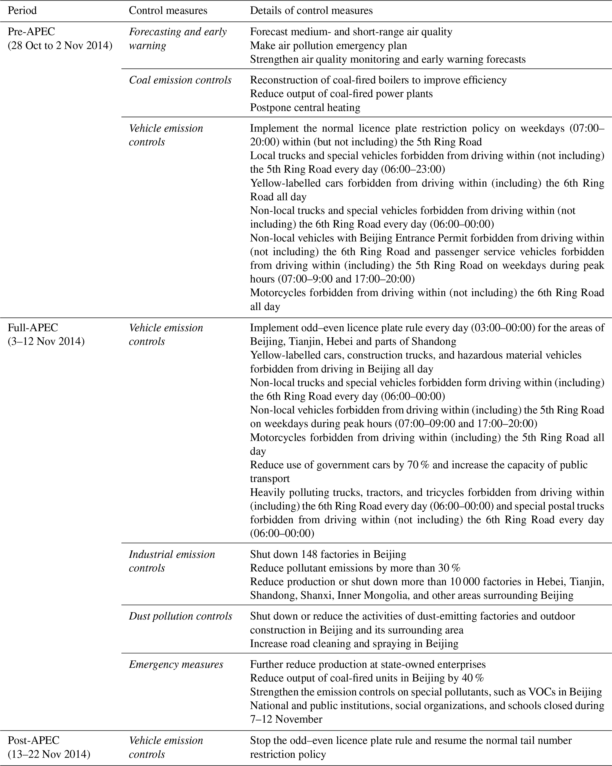
On-road measurements were carried out around the 4th Ring Road of Beijing from 2 October to 22 November 2014. The APEC summit was held in Beijing from 5 to 11 November 2014. The Chinese government implemented a series of air pollution control policies to ensure good air quality in Beijing during the APEC summit. The Ministry of Environmental Protection of China formulated “the assurance program of air quality during the APEC summit”. The area covered by air pollution control policies included Beijing, Tianjin, Hebei, Shanxi, Inner Mongolia, and Shandong. The air pollution control policies were implemented in a stepwise manner before the APEC summit commenced. In this study, the observation period (28 October to 22 November 2014) was divided into three time periods according to when air pollution control policies were implemented, with a particular focus on the odd–even vehicle licence plate rule (i.e. only vehicles with odd last digits on their licence plates were allowed to drive on one day, only those with even last digits on the next day, and so on), imposed during the APEC summit.

• Pre-APEC (28 October–2 November 2014). During this period, control policies on vehicles and coal combustion were implemented gradually. An early warning system for air quality was established, with a series of contingency plans developed that would be put in place if heavy pollution episodes occur during the 2014 APEC summit.

• Full-APEC (3–12 November 2014). During this period, air pollution control policies on coal combustion, industrial, dust, and vehicle emissions were fully implemented. Some heavily polluting industrial factories were shut down. Strict temporary vehicle emission control policies and the odd–even vehicle licence plate rule were also imposed during this period.

• Post-APEC (13–22 November 2014). During this period, the odd–even vehicle licence plate rule was lifted and the normal licence plate restriction policy was resumed. Industrial factories gradually resumed production.

Further details of these air pollution control policies are given in Table 1.

Table 1 Air pollution control measures implemented during the pre-APEC, full-APEC, and post-APEC periods.

Over the 26 d of observations, on-road mobile measurements were conducted during 44 circuits of the 4th Ring Road (Table S1 in the Supplement). The morning observation period was from 09:50 to 12:00 LT and the night-time was from 01:00 to 02:30 LT. The observation vehicle started around 10:00 LT in the morning, mainly for better development of the atmospheric boundary layer and the reduced traffic congestion during this time (i.e. after the morning rush hour) (Tao et al., 2007; Han et al., 2014). We also conducted on-road mobile measurements during the night-time to explore the differences in vehicle emission control policies between daytime and night-time (Table 1). According to Bukowiecki et al. (2002), the probability of measured results being affected by self-pollution is only 5 % when the driving speed of a mobile laboratory exceeds 5 km h⁻¹. The driving speed in this study was kept at ∼60 km h⁻¹ to maintain a constant sampling flow rate and reduce self-pollution. The effects of self-pollution can thus be neglected for most of the observations. The total driving times for the measurements were around 1–1.5 h, except for 14, 18, 20, and 21 November 2014, during which there was substantial traffic congestion that led to longer measurement time.

2.2 The wavelet transform method (WTM)

The WT is a powerful technique for time–frequency analysis and is widely used in seismic data analysis, transient signal analysis, and other signal processing applications (Tian et al., 2014; Domingues et al., 2005; Kang et al., 2007). Unlike the STFT, which decomposes a signal into a set of equal bandwidth basis functions in the spectrum, the WT provides a decomposition based on constant-Q (equal bandwidth on a logarithmic scale) basis functions with improved multi-resolution characteristics in the time–frequency plane (Akansu et al., 2010). The WT maps the function f(t) in L²(R) to another signal W_f(a,b) in L²(R²), where a and b are continuous and referred to as the scaling and shift parameters, respectively. The continuous WT of a time series f(t) is defined as follows:

$$\begin{array}{}\text{(1)}& {\displaystyle }\begin{array}{rl}{W}_f\left(a,b\right)& =\left\{f\left(t\right),{\mathit{\psi }}_{ab}\left(t\right)\right\},\\ & ={\int }_{-\mathrm{\infty }}^{\mathrm{\infty }}f\left(t\right){\stackrel{\mathrm{‾}}{\mathit{\psi }}}_{ab}\left(t\right)\mathrm{d}ta>\mathrm{0},\end{array}\text{(2)}& {\displaystyle }{\mathit{\psi }}_{ab}\left(t\right)={\displaystyle \frac{\mathrm{1}}{\sqrt{a}}}\mathit{\psi }\left({\displaystyle \frac{t-b}{a}}\right),\end{array}$$

where f(t) represents the time series of a signal, ψ(t) is the mother wavelet function, and ${\stackrel{\mathrm{‾}}{\mathit{\psi }}}_{ab}\left(t\right)$ is the conjugate complex of ψ_ab(t). Selecting the appropriate mother wavelet function (ψ(t)) is key to the WTM. The continuous scaling and shift parameters (a,b) make the continuous WT quite redundant and result in high computational cost. Thus, the discrete WT, which uses discrete values of scale (j) and localization (k), was used instead. If we let the sampling grid $a=a_{\mathrm{0}}^j$ and b= $k{b}_{\mathrm{0}}{a}_{\mathrm{0}}^j$, the discrete WT is defined as follows:

$$\begin{array}{}\text{(3)}& \mathit{\left\{}{\mathit{\psi }}_{jk}\right(t\left)\mathit{\right\}}={\mathit{\psi }}_{jk}\left(t\right)=a_{\mathrm{0}}^{\frac{-j}{\mathrm{2}}}\mathit{\psi }\left(a_{\mathrm{0}}^{-j}t-k{b}_{\mathrm{0}}\right).\end{array}$$

The commonly used mother wavelet functions include Haar (denoted by “haar”), Daubechies (“dbN”, where N is an integer), Coiflet (“coifN”), Symlets (“symN”), Morlet (“morl”), Mexican Hat (“mexh”), and Meyer (“meyr”) (Fig. S1 in the Supplement). In this study, the Daubechies wavelet functions (“dbN”) were chosen as mother wavelet functions to conduct the discrete WT, mainly based on the similarity principle (Daubechies et al., 1992; Sang and Wang, 2008; Thornhill et al., 2010) (Fig. S1). The number of decomposition levels was set in the range 5–9 based on considerations of computational costs, information integrity, and boundary effects. Different decomposing schemes were conducted to investigate how the parameters, such as the mother wavelet function and decomposition level, affected the results of the WTM. MATLAB (R2016a) was used to conduct the WT decomposition.

After WT decomposition, the original signals (measured on-road pollutant concentrations in this study) were divided into low- and high-frequency components that reflect the approximated and detailed information of the original signals, respectively (Fig. S2). The results of the WT decomposition included both positive and negative values for the high-frequency component, which were due to the mother wavelet vibrating near zero. To reconcile this problem, the high-frequency component was moved up using a REF-line (i.e. reference, based on a running 5 min minimum of the raw data) and the low-frequency component was moved down in a homologous manner (Fig. S3). Through WT decomposition and REF-line adjustment, we obtained the results of the WTM as follows:

$$\begin{array}{}\text{(4)}& C_{\mathrm{Total}}=C_{\mathrm{L}\mathrm{\_}\mathrm{freq}.}+C_{\mathrm{H}\mathrm{\_}\mathrm{freq}.}=C_{\mathrm{bg}.}+C_{\mathrm{veh}.},\end{array}$$

where C_Total is the measured on-road pollutant concentrations and corresponds to their original signals and C_{L_freq.} and C_{H_freq.} are the low- and high-frequency components of the WTM, respectively. For the pollutants typically related to vehicle emissions, such as NO, NO_x, BC, and CO, C_{L_freq.} is equivalent to their on-road background concentrations (C_bg.) and C_{H_freq.} is equivalent to the contributions from immediate vehicle emissions (C_veh.). The vehicle emission control policies implemented during the full-APEC period could have affected both traffic flow and the vehicle fleet profile (which could change emission intensities) and thus could influence the contributions of vehicle emissions to pollutant concentrations. Therefore, the high-frequency component of the WTM can be used to evaluate the vehicle emission control policies.

To verify the suitability and efficacy of the WTM in the signal decomposition of on-road-measured pollutant concentrations, the results of the WTM were compared with the moving low-percentile method (MLPM) and observations at the PKU site. The moving low-percentile method (MLPM) is developed by Bukowiecki et al. (2002) and is a tested method for separating concentration of on-road background (i.e. C_bg. or C_{L_freq.}) and concentration from immediate vehicle emissions (i.e. C_veh. or C_{H_freq.}), which is useful in evaluation of on-road emission reduction.

3 Results and discussion

3.1 Results of on-road mobile measurements

We give an overview of the results of the on-road mobile measurements in this section. Both meteorological conditions and the temporal and spatial distributions of air pollutants were investigated.

Meteorological conditions, especially wind direction (WD) and wind speed (WS), play key roles in the dispersal and transport of air pollutants. Comprehensive understanding of the transport of air pollutants between megacities and their surrounding areas and separation of the contributions of meteorological conditions and air pollution control policies is important for the objective evaluation of such control policies (Li et al., 2016, 2019; Liang et al., 2017).

As shown in Fig. 2, the meteorological conditions (measured at the Nanjiao site; see Fig. 1) varied over the course of the measurement period. The average wind speed during the pre-APEC period was 1.8 m s⁻¹, and there were strong contributions from the northwest (∼25 %) and northeast (∼30 %) wind sectors. The average wind speed during the full-APEC period was 2.1 m s⁻¹, which is higher than that during the pre- and post-APEC periods. The prevailing winds during the full-APEC period were from the northwest (∼20 %) and southwest (∼25 %). The average wind speed for the post-APEC period was 1.5 m s⁻¹, which is the lowest of the three periods. The prevailing winds during the post-APEC period were from the northeast (∼35 %) and southwest (∼25 %). For Beijing, the northwest sector generally corresponds to clean air masses, while the northeast and south wind sectors have many hotspots of air pollutant emissions (Wu et al., 2011; Lin et al., 2011; Li et al., 2016). Thus, the WD and WS during the post-APEC period were less favourable for the dispersal of air pollutants than during the other two periods, whereas the dispersion and transport conditions during the pre- and full-APEC periods were virtually indistinguishable.

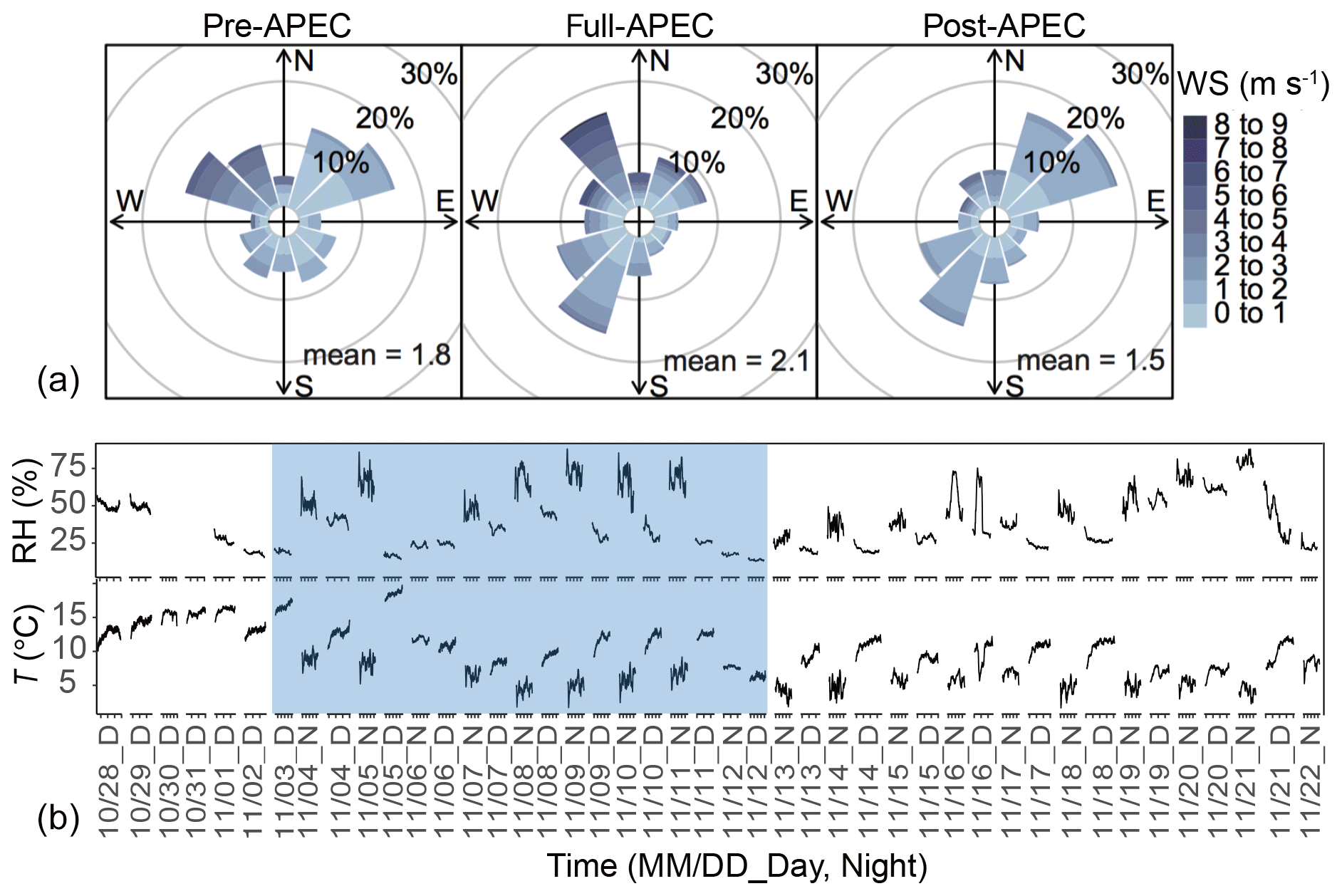
Figure 2 (a) Rose plots of wind direction (WD) and wind speed (WS) measured at the Nanjiao site during the pre-APEC (24 October to 2 November 2014), full-APEC (3–12 November 2014), and post-APEC (12–22 November 2014) periods. (b) Time series of the on-road observed temperature (T) and relative humidity (RH) during the observation period; the shaded blue area indicates the full-APEC period. APEC refers to the 2014 Asia-Pacific Economic Cooperation summit.

As shown in Fig. 2, RH was higher during the full- and post-APEC periods relative to the pre-APEC period, especially at night. T decreased significantly after 6 November 2014, with a maximum of < 15 ^∘C in the daytime and a minimum of ∼5 ^∘C at night. Similar to WD and WS, RH and T during the post-APEC period were less conducive to good air quality than during the other two periods.

In this study, we have considered the impact of meteorological conditions in the experimental design. All observation trips started at the same period of 1 day (i.e. about 10:00 LT in the daytime and about 01:00 LT in the night-time), with relatively stable atmospheric boundary layer during the selected observation period, which can eliminate the meteorological influence to some extent. We chose the wide main road (i.e. the 4th Ring Road) for observation to reduce the impact of microscale turbulence and meteorological disturbances, which is complex on narrow roads. Meanwhile, direct measurements of wind speed and wind direction from the mobile lab during driving may have large deviations (Johansson, 2009; Wang et al., 2011). The observation data of wind speed and direction at the ground-based site (such as the Nanjiao site) is hourly mean data, with low time resolution and limited spatial representation. It is difficult to obtain high time resolution and accurate meteorological data matching the concentration of gaseous pollutants. The lack of high-time-resolution meteorological data make it difficult to accurately evaluate and eliminate the meteorological impacts. The short-term microscale meteorology has little effect on our assessment results, and the discussion and accurate quantification of microscale meteorological influences are beyond the scope of this study. Here we assumed that the high-frequency component is confined to much shorter timescales than those of the meteorological factors, and that changes in meteorological conditions were reflected only in the low-frequency component, such that changes in meteorological conditions did not influence our evaluation of control polices.

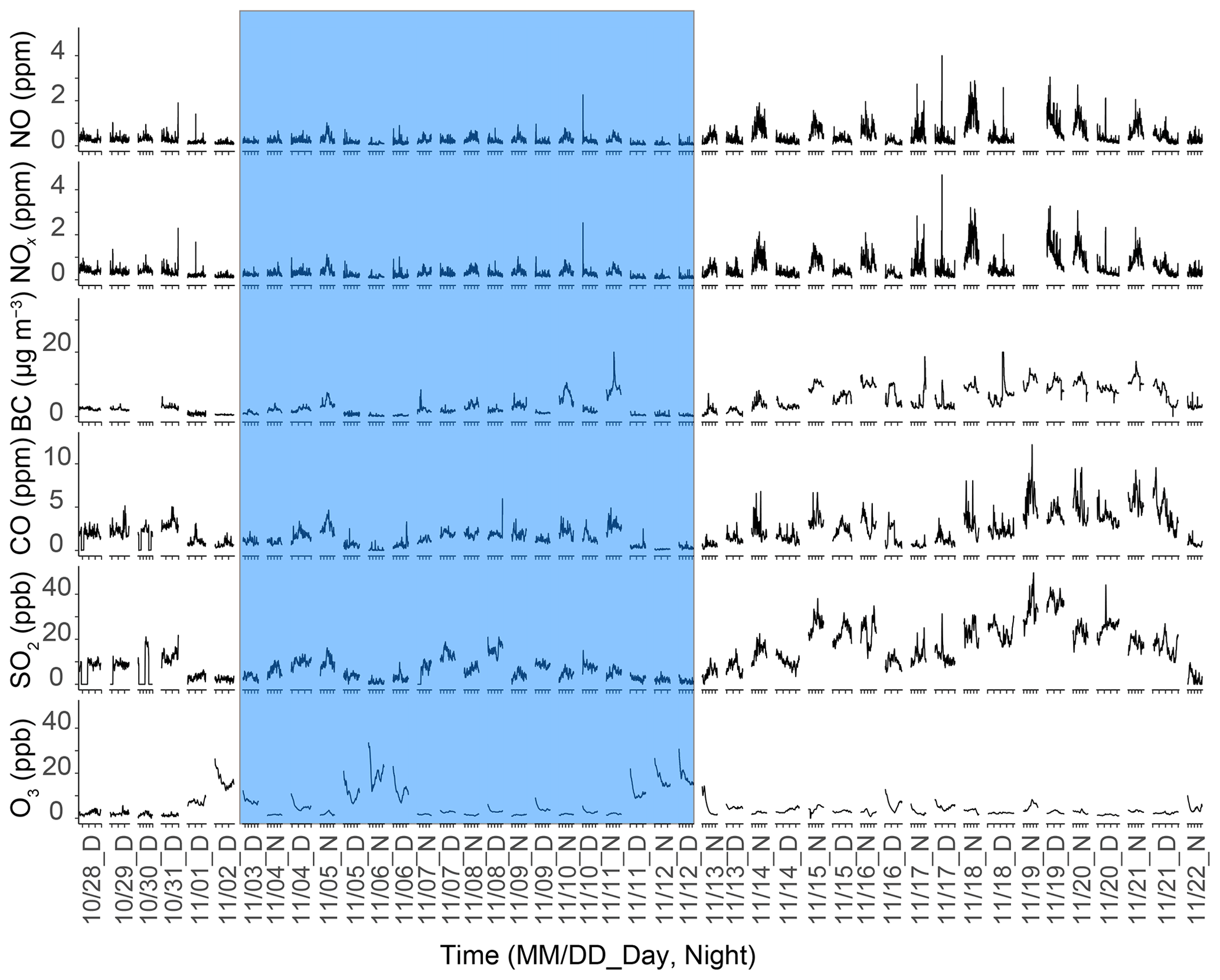
Figure 3 Time series of on-road mobile measurements of NO, NO_x, black carbon (BC), CO, SO₂, and O₃ concentrations around the 4th Ring Road of Beijing from 28 October to 22 November 2014. The shaded blue area indicates the full-APEC period.

Figure 3 shows time series of NO, NO_x, BC, CO, SO₂, and O₃ observations from 28 October to 22 November 2014, for which the mean ±1 standard deviation (SD) concentrations were 337.7±330.4 ppb, 416.6±373.2 ppb, 4.3±3.7 µg m⁻³, 2.1±1.6 ppm, 11.8±9.5 ppb, and 5.0±5.0 ppb, respectively (Table 2). The measured concentrations are higher than those in Europe and America, which indicates that the air pollution problem in Beijing is among the worst in the world (Zhu et al., 2016; Hagemann et al., 2014; Padró-Martínez et al., 2012; Westerdahl et al., 2005). For example, on-road mobile measurements in the North China Plain (NCP) during summer 2013 yielded mean NO_x, BC, CO, and SO₂ concentrations of 422 ppb, 5.8 µg m⁻³, 1006 ppb, and 15 ppb, respectively (Zhu et al., 2016). The mean concentrations of NO_x for mobile measurements made during 2010 in Karlsruhe, Germany, were 20 ppb in inner-city areas and 30 ppb in traffic-influenced locations (Hagemann et al., 2014). The measured average on-road concentrations of NO, NO_x, BC, and CO were about 30 ppb, 50 ppb, 1 µg m⁻³, and 0.5 ppm, respectively, in Somerville, USA, during 2009–2010 (Padró-Martínez et al., 2012). The average measured on-road concentrations of NO_x were 140 and 230–470 ppb on arterial roads and freeways, respectively, in Los Angeles, USA, during spring 2003 (Westerdahl et al., 2005). The low level of O₃ concentration in this study (5.0±5.0 ppb) is mainly due to the titration of O₃ by NO with high concentration.

Table 2 The mean concentrations of pollutants measured around the 4th Ring Road of Beijing and their relative changes between the pre-APEC, full-APEC, and post-APEC periods.

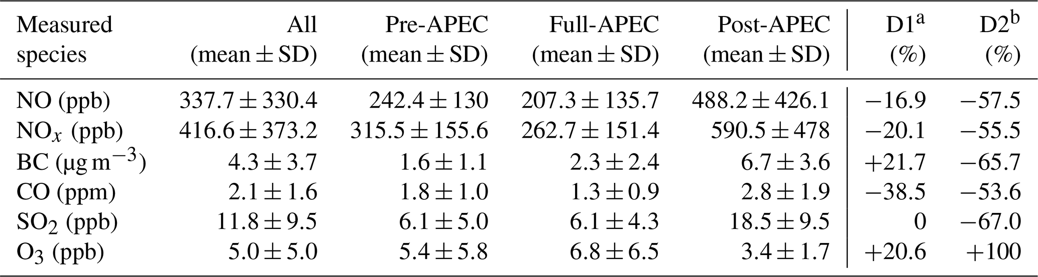
SD: standard deviation. ^a D1 = (full-APEC − pre-APEC) ∕ pre-APEC. ^b D2 = (full-APEC − post-APEC) ∕ post-APEC.

The mean ±1 SD concentrations of NO, NO_x, BC, CO, SO₂, and O₃ during the full-APEC period were 207.3±135.7 ppb, 262.7±151.4 ppb, 2.3±2.4 µg m⁻³, 1.3±0.9 ppm, 6.1±4.3 ppb, and 6.8±6.5 ppb, respectively, which reflect substantial decreases compared to those in the pre-APEC period, and are much lower than those in the post-APEC period (Table 2). The decreases in pollutant concentrations during the full-APEC period are partially attributed to the implementation of air pollution control policies, in addition to changes in local emissions (e.g. commencement of the heating season in the post-APEC period) and the regional transport of air pollutants.

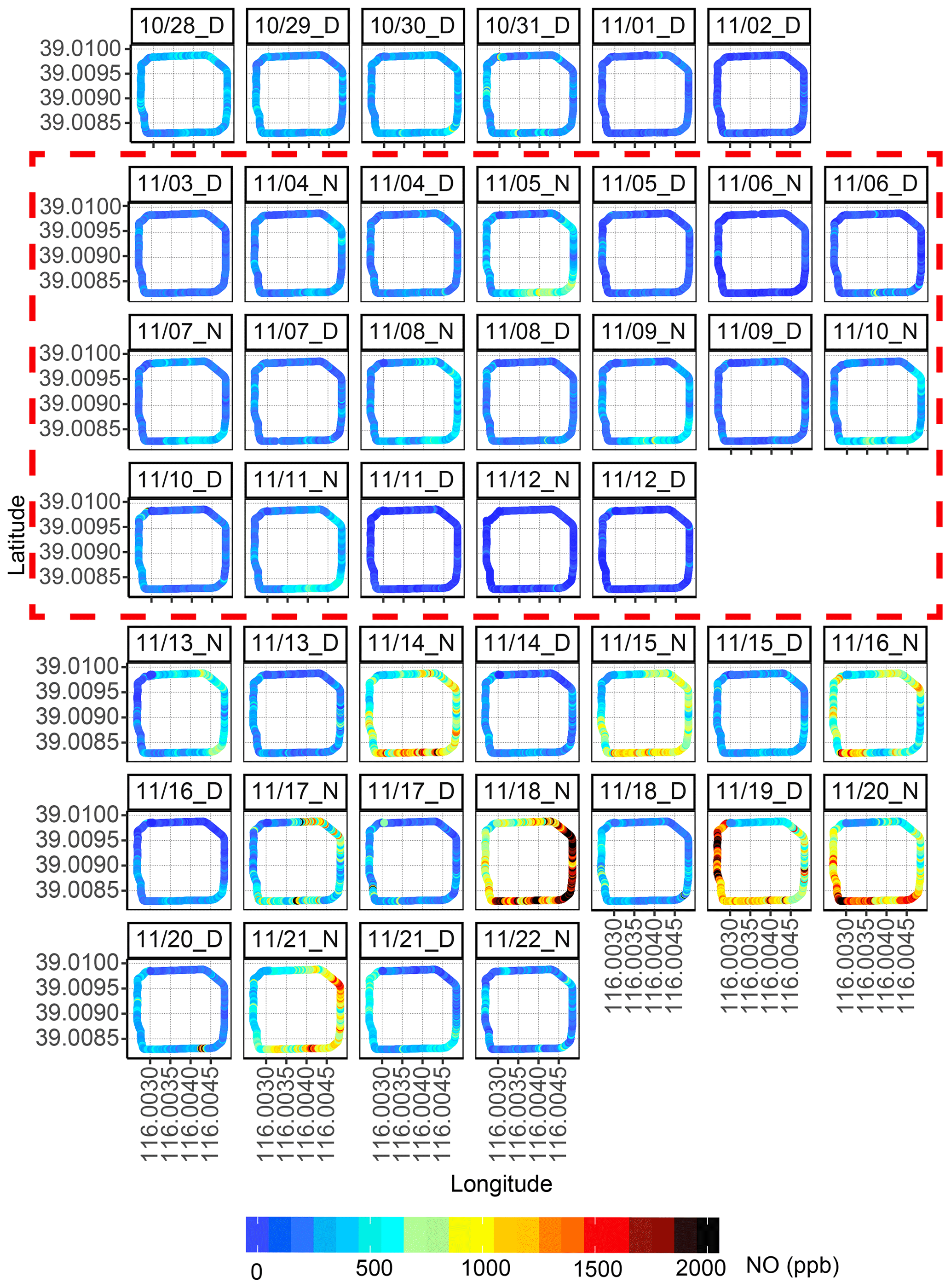
Figure 4 The spatial distributions of NO around the 4th Ring Road of Beijing from 28 October to 22 November 2014. The subtitle for each circuit indicates the observation time in the form “MM/DD_Day, Night”. The dotted red rectangle area indicates the full-APEC period.

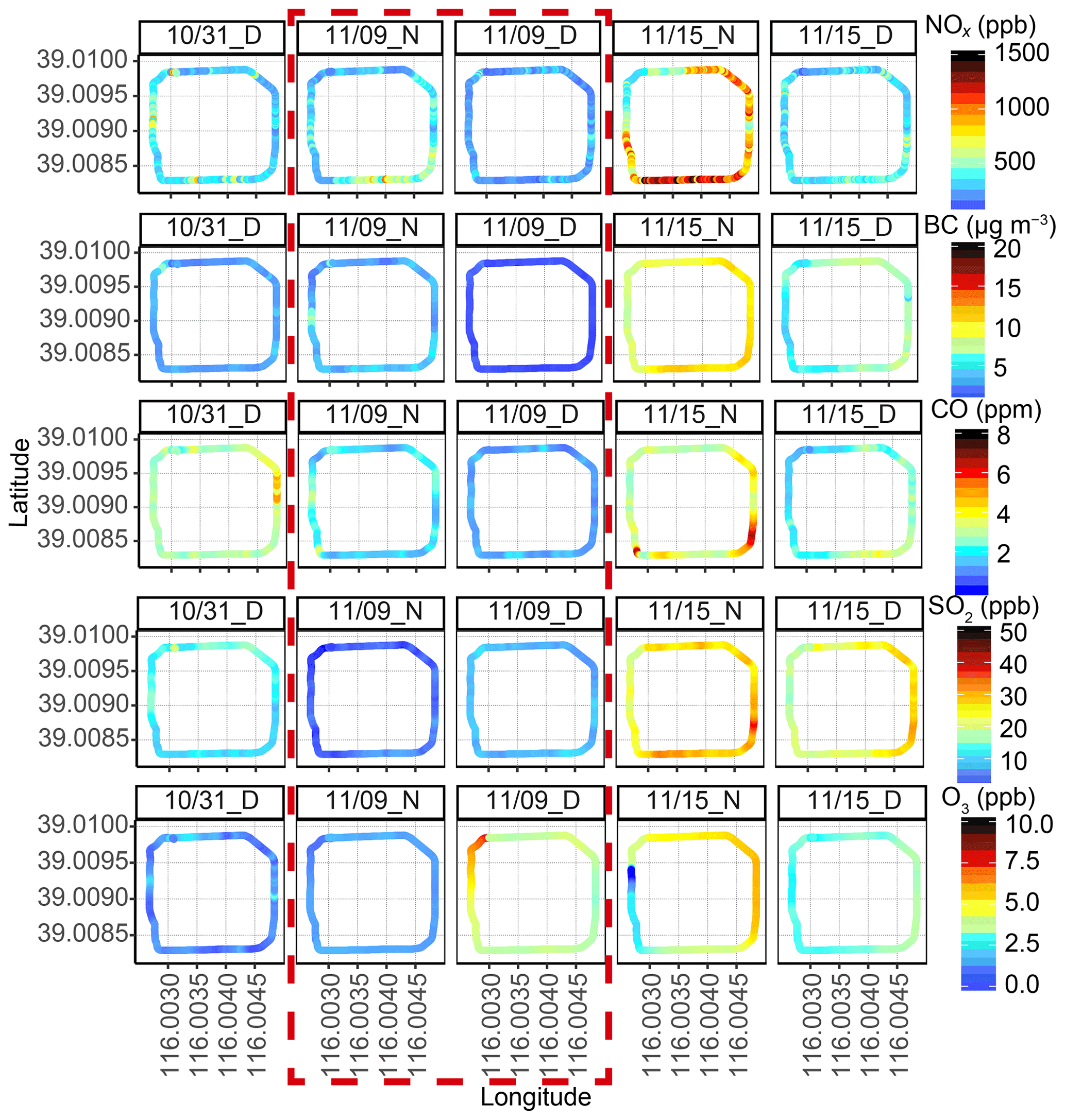
Figure 5 The spatial distributions of NO_x, BC, CO, SO₂, and O₃ observed around the 4th Ring Road of Beijing. The data from 31 October, 9 November and 15 November 2014 were selected to represent the pre-APEC, full-APEC, and post-APEC periods, respectively. The subtitle for each circuit indicates the observation time in the form “MM/DD_Day, Night”. The dotted red rectangle area indicates the full-APEC period.

Figures 4 and 5 show the spatial distributions of pollutants around the 4th Ring Road of Beijing during the observation period. In general, for NO, NO_x, and CO, the spatial distributions were non-uniform with several short-term spikes observed during circuits of the ring road. The spatial distributions of BC, SO₂, and O₃ were relatively uniform compared to those of NO, NO_x, and CO.

The measured on-road concentrations of NO (Fig. 4) and NO_x (data not shown) were > 500 ppb on some polluted days. These high values were often found in the southern part of the 4th Ring Road and were observed during both daytime and night-time. For example, during the nights of 14, 15, 18, and 21 November 2014, the concentrations of NO and NO_x in the eastern part of the ring road were > 500 ppb, and sometimes even > 1000 ppb. During the nights of 16 and 20 November 2014 and in the daytime on 16 November 2014, the concentrations of NO and NO_x in the western part of the ring road were also high, while their concentrations in the northwestern part were relatively low.

A total of 3 days, namely 31 October, 5 November and 15 November 2014, were selected based on the similar meteorological conditions to explore the temporal and spatial distributions of air pollutants (Fig. 5). The meteorological conditions are unfavourable for the dispersion of atmospheric pollutants on these 3 days. The weather circulation field is a homogenous or weak pressure field, the wind speed near the ground is small, and the atmospheric static stability is high. The average hourly wind speed on 31 October, 9 November and 15 November 2014 was 1.19, 1.28 and 1.07 m s⁻¹, respectively. The measured on-road concentrations of NO, NO_x, BC, and CO were higher during night-time than during daytime. The measured on-road concentrations of BC increased to > 10 µg m⁻³ and even 20 µg m⁻³ in some parts of the 4th Ring Road of Beijing during the post-APEC period, such as during the nights of 15–21 November 2014 and in the daytime on 16, 19, and 20 November 2014. High BC concentrations were often found in the southeastern part of the ring road. From 18 to 21 November 2014, the concentration of on-road-measured CO reached up to 10 ppm in some parts of the ring road. The concentration of CO was generally higher in the southern part than the northern part of the ring road. High concentrations also appeared in the northwest and northeast. The measured on-road concentration of SO₂ sometimes increased to above 20 ppb during the post-APEC period, such as during the nights of 15–16 and 18–21 November 2014 and in the daytime on 16 and 18–20 November 2014. In contrast to other pollutants, there was no significant difference in the concentrations of SO₂ between daytime and night-time. The spatial distribution of SO₂ shows more obvious regional characteristics, with a lack of short-term peaks in its concentration. The temporal distribution of O₃ was quite different from other pollutants, in that its concentration increased significantly during the full-APEC period. During the night-time of 6 November 2014 and in the daytime on 2 and 12 November 2014, the on-road concentrations of O₃ increased to >20 ppb. In general, daytime O₃ concentrations were higher than those during night-time. High concentrations of O₃ were often found in the northeastern, southeastern, and southwestern parts of the ring road.

Table 3 The on-road emission concentrations obtained from the WTM for NO, NO_x, BC, CO, SO₂, and O₃ with different mother wavelet functions (i.e. db4–db8) and decomposition levels (5–9 levels).

^* SD is the SD of on-road concentrations estimated using different schemes in the WTM.

We obtained the spatial distribution characteristics of pollutants around the 4th Ring Road of Beijing using on-road mobile measurements. The concentrations of NO_x, BC and O₃ showed some elevated values in the southern part of the 4th Ring Road. It is speculated that the elevated values of NO_x and BC in the southern part of the 4th Ring Road is mainly due to busy traffic and that the concentrated industries are also one of the reasons (Cheng et al., 2013; Wang et al., 2009; Westerdahl et al., 2009; Zhu et al., 2016). The high ozone values in the southern part are mainly due to the regional transport from southern area where ozone photochemical reaction is strong (Li et al., 2016). The concentrations of NO, NO_x, BC, CO, and SO₂ during the full-APEC period were lower than those during the pre-APEC period and substantially lower than the post-APEC period. The reasons for the dramatic increases in pollutant concentrations after the APEC summit may be attributed to increases in emissions due to the stoppage of air pollution control policies (Table 1), increases in the energy demand for heating due to temperature reductions (Liu et al., 2016), and unfavourable meteorological conditions (Fig. 2). The increase in O₃ concentrations during the full-APEC period was related to reductions in the NO-titration effect, i.e. due to decreases in NO concentrations (Wang et al., 2017). The concentrations of NO, NO_x, BC, and CO during night-time were higher than those during daytime, which may be partially attributed to decreases in the boundary layer height and increased truck emissions during night-time (Fan et al., 2016). SO₂ concentrations showed no significant difference between the night-time and daytime, which is consistent with previous observations of a double peak in the diurnal profile of SO₂ observations in Beijing (Lin et al., 2012).

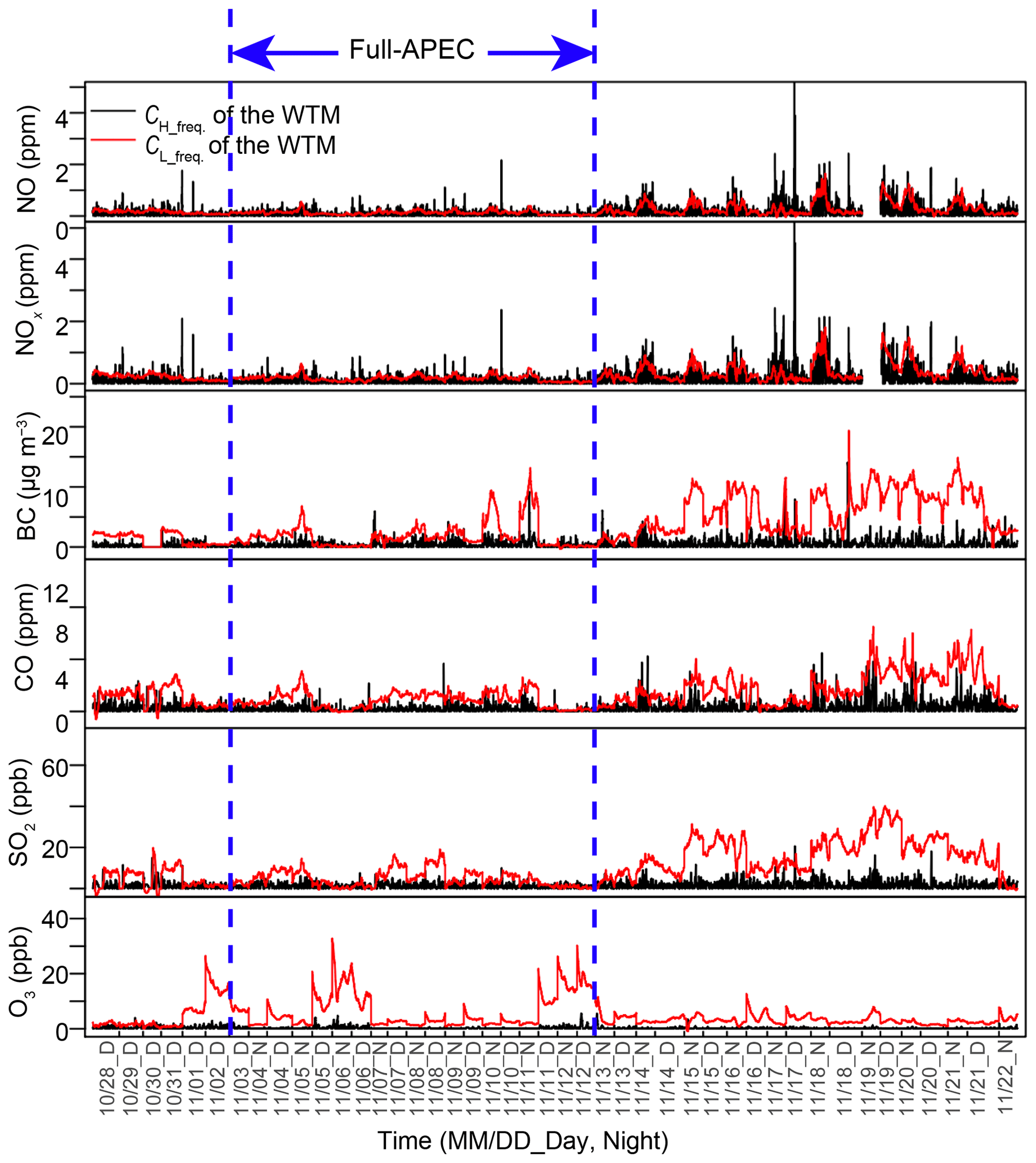
Figure 6 Time series of the decomposition results of the wavelet transform method (WTM) for NO, NO_x, BC, CO, SO₂, and O₃ (db6, eight levels; see text for details). The black lines represent the high-frequency components of the WTM, which should originate from immediate vehicle emissions. The red lines represent the low-frequency components of the WTM, which correspond to the atmospheric background plus accumulated on-road emissions.

Vehicle emissions make important contributions to the concentrations of NO, NO_x, BC, and CO (Zhou et al., 2010; Cheng et al., 2013), thus on-road measurements of these species have previously been used to investigate vehicle emissions (Wang et al., 2009; Zhu et al., 2016). Short-term peaks in on-road-measured NO, NO_x, and CO concentrations reflect their immediate emissions from on-road vehicles (Westerdahl, et al., 2009; Han et al., 2014). However, in the present work, the short-term peaks in BC and CO were not as obvious as those of NO and NO_x. The reasons for these differences are as follows. First, the lifetimes of NO and NO_x in the atmosphere are only a few hours (Li et al., 2016), which are much shorter than those of BC and CO with lifetimes of 1 week (Samset et al., 2014) and nearly 1 month (Li et al., 2016), respectively. Therefore, NO and NO_x concentrations were more sensitive to the impacts of immediate vehicle emissions compared to BC and CO. Second, the response times of instruments usually used for BC and CO measurements are longer than those for NO and NO_x, which limits mobile measurements in their ability to capture instantaneous vehicle emission plumes during on-road observations.

On-road mobile measurements can be used to obtain spatial distributions of pollutants with high time resolution over large areas. Here we investigated the spatial distributions of pollutants around the 4th Ring Road of Beijing to understand the distribution characteristics of different pollutants. According to their distribution features, we found that the typical pollutants NO, NO_x, BC, and CO (NO and NO_x in particular) were suitable for the evaluation of vehicle control policies in this study. We also observed differences in pollutant behaviour between daytime and night-time.

3.2 Results of the WTM and comparison with other methods

To select appropriate parameters for the WTM, we chose different mother wavelet functions (db4–db8) and numbers of decomposition levels (5–9 levels) to carry out the WT. The average high-frequency components (i.e. C_{H_freq.}) of the WTM for NO, NO_x, BC, CO, SO₂, and O₃ using different mother wavelet functions and decomposition levels are listed in Table 3. We first conducted the WTM using a fixed mother wavelet function (db4) and varied the number decomposition levels (5–9 levels). The results in Table 3 showed that the decomposition result was insensitive to the number of decomposition levels. We carefully investigated the time series of the WT results and found that an eight-level decomposition could describe the characteristics of on-road vehicle emissions correctly (Westerdahl et al., 2009; Han et al., 2014). We then conducted the WTM with a fixed decomposition level (eight levels) and varied the mother wavelet function (db4–db8). Considering the head–tail effect of the WT, we chose db6 as the most appropriate mother wavelet function (Figs. S2 and S3). The SD in the WTM for NO, NO_x, BC, and CO was only 1.1, 1.2, 0, 0.1, 0.3, 0.1, respectively, which highlights the stability of the WTM. It should be noted that SO₂ and O₃ are not good tracers for vehicle emissions. They were presented in the general discussion section as a measured pollutant in our experiment. However, as we discuss the on-road emission reduction, SO₂ and O₃ is not included.

Figure 6 shows the time series obtained from the WTM for NO, NO_x, BC, CO, SO₂, and O₃ during the observation period, using db6 as the mother wavelet function and eight levels of decomposition. The measured on-road pollutant concentrations were decomposed into a high-frequency component (C_{H_freq.}) and a low-frequency component (C_{L_freq.}). For the typical pollutants NO, NO_x, BC, and CO, C_{L_freq.} is equivalent to C_bg. and C_{H_freq.} is equivalent to C_veh., as discussed previously. As shown in Fig. 6, C_{H_freq.} could only account for a small proportion of the measured concentrations of SO₂ and O₃. The variations in C_{H_freq.} (C_veh.) for NO and NO_x were the largest among the measured pollutants, whereas the variations in C_{H_freq.} (C_veh.) for CO and BC were not as significant.

To verify the accuracy and efficacy of the WTM, the following techniques were used. First, we used the MLPM to separate C_veh. and C_bg. (Fig. 7) and compared this to the results of the WTM. Second, C_{L_freq.} from the WTM was compared with the pollutant concentrations observed at the PKU site (Figs. 8 and S1).

The MLPM is traditionally used to separate C_veh. and C_bg. (Bukowiecki et al., 2002). In this study, we also used the MLPM and compared its results with the WTM. Figure 7 shows the time series of MLPM decomposition results for NO, NO_x, BC, and CO. C_bg. was regarded as the moving 5 min fifth percentiles of pollutant concentrations. C_veh. was estimated by subtracting C_bg. from C_Total. Table 4 shows the decomposition results of the MLPM for different schemes. The correlation coefficients (R²) between C_veh. decomposed by the WTM and the MLPM were 0.996, 0.994, 0.894, and 0.840 for NO, NO_x, CO, and BC, respectively (Fig. S4). This comparison indicates the agreement of both methods in signal decomposition (Fig. S4), but the decomposition results show that the WTM is more stable than the MLPM (Figs. 6 and 7, Tables 3 and 4).

Table 4 The mean on-road emission concentrations estimated using the moving low-percentile method (MLPM) for NO, NO_x, BC, CO, SO₂, and O₃ with different time windows (i.e. 1–10 min) and percentiles (i.e. 1 %, 5 %, and 10 %).

^* SD is the SD of on-road concentrations estimated using different schemes in the MLPM.

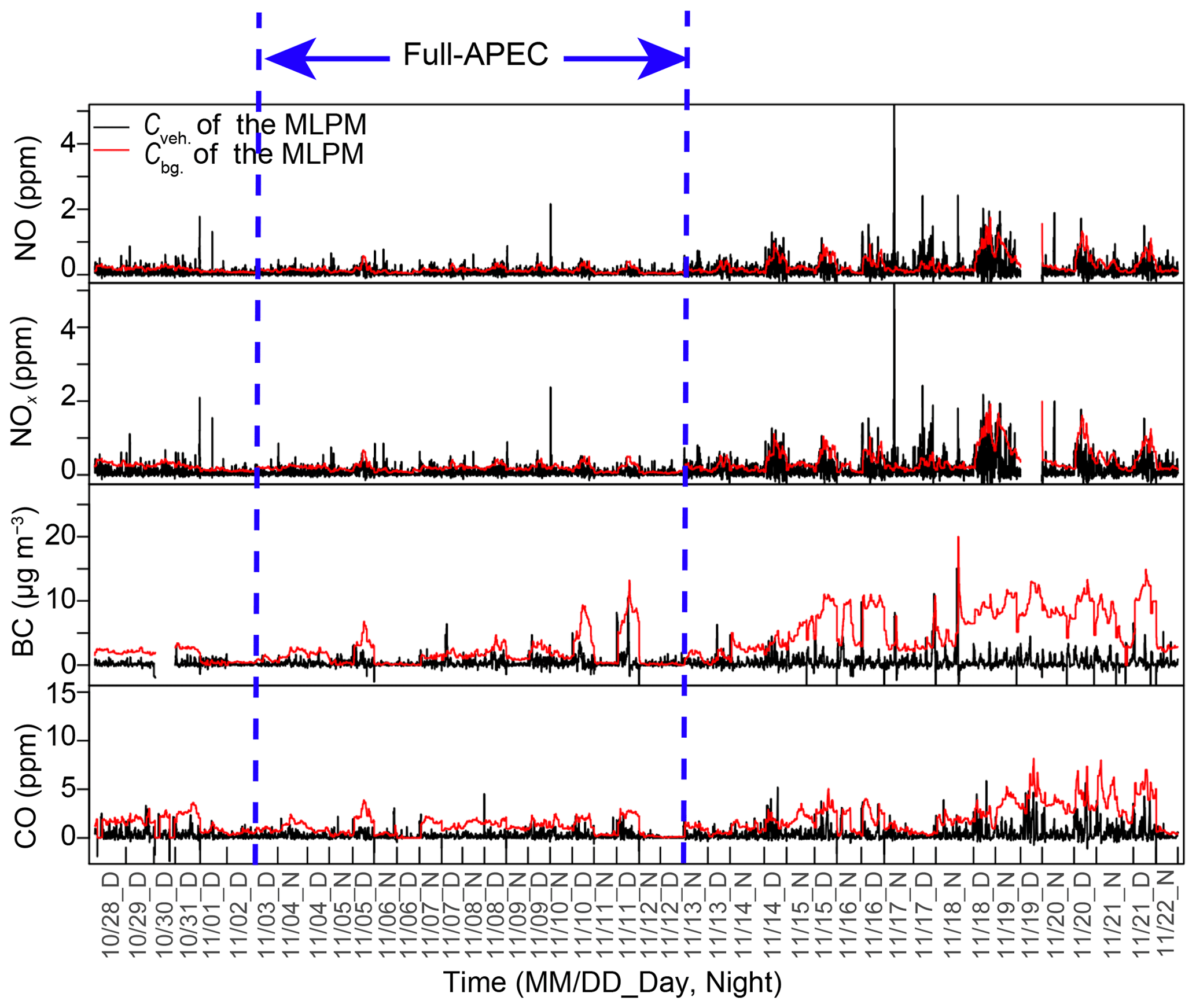
Figure 7 Time series of the separation results using the moving low-percentile method (MLPM) for NO, NO_x, BC, CO, SO₂, and O₃. The red lines represent moving 5 min fifth percentiles of the measured pollutant concentrations to determine on-road background concentrations. The black lines represent estimated on-road emission concentrations, which were obtained by subtracting the background concentrations from the original concentrations.

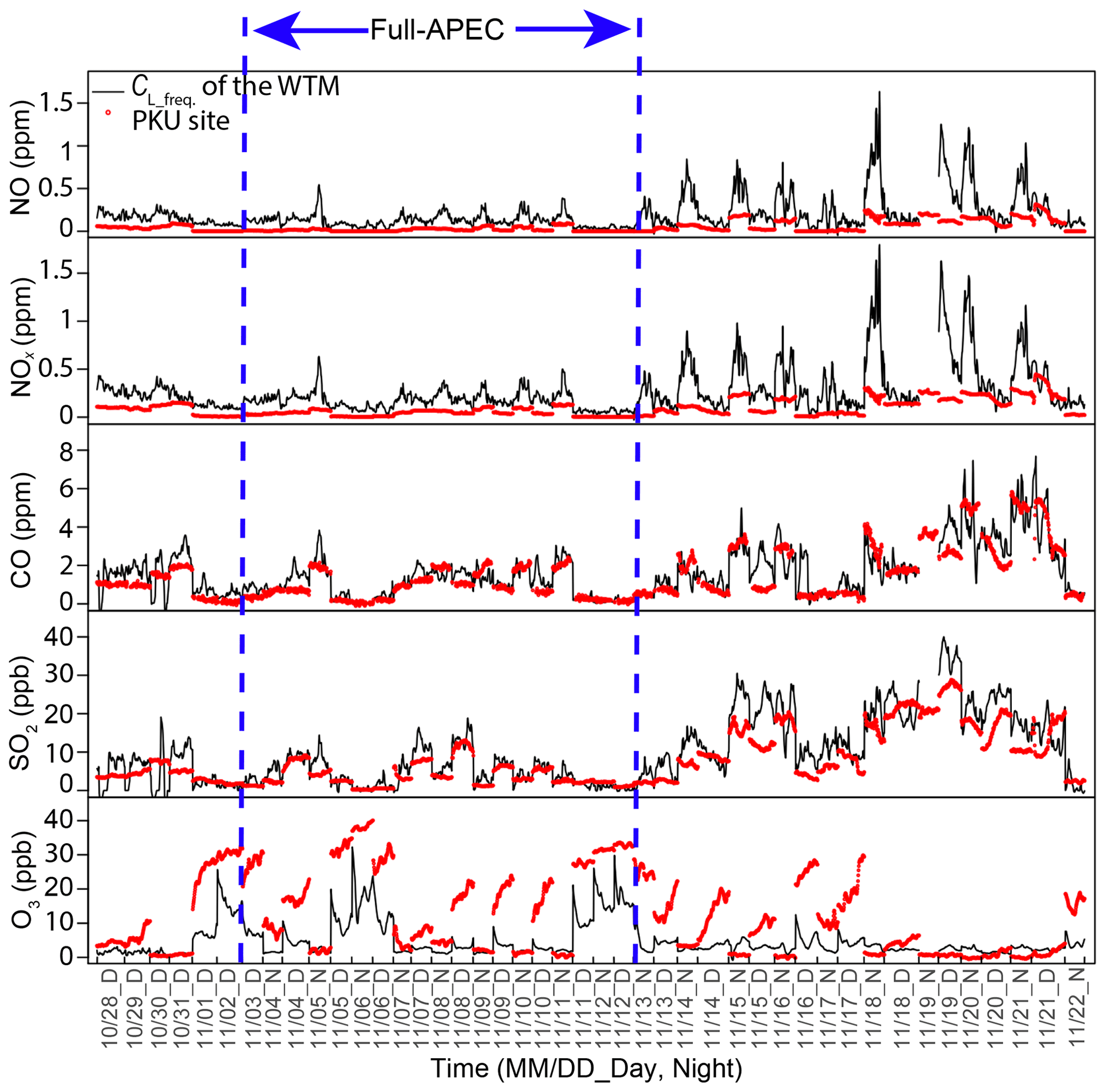
Figure 8 Comparisons between time series of the low-frequency components of the WTM and concentrations observed at the PKU site for NO, NO_x, BC, CO, SO₂, and O₃. The black lines represent the low-frequency components of the WTM. The red line represents the 1 min average concentrations of pollutants observed at the PKU site.

Figure 8 shows the comparison of C_{L_freq.} obtained by the WTM with observed concentrations of NO, NO_x, CO, SO₂, and O₃ at the PKU site. The variations in on-road background concentrations obtained by the WTM were similar to the concentrations observed at the PKU site. The correlation coefficients (R²) between C_{L_freq.} from the WTM and PKU site observations were 0.748, 0.715, 0.912, 0.927, and 0.752 for NO, NO_x, CO, SO₂, and O₃, respectively (Fig. S5). However, for NO and NO_x, the absolute values of C_{L_freq.} (C_bg.) from the WTM were higher than the concentrations observed at the PKU site. This is attributed to the following reasons. First, PKU is a fixed ground-based site with limited regional representation, but the on-road measurement covered large areas. Second, C_bg. obtained by the WTM for NO and NO_x included both their atmospheric background concentrations and their accumulated concentrations from vehicle emissions. The above comparison indicates that the WTM could be a feasible way to separate C_veh. from the on-road-measured concentrations of air pollutants.

3.3 Case study: evaluation of vehicle emission control policies

Air pollution control policies were gradually implemented prior to the APEC summit and were quickly abandoned after the summit. Stricter vehicle emission control policies were implemented during the full-APEC period, such as the odd–even licence plate rule instead of the normal licence plate restriction policy, and limits on driving time and range were more stringent for non-local vehicles, trucks, and government cars. Table 5 shows the mean ±1 SD C_veh. of the WTM and the relative changes in NO, NO_x, BC, and CO during different observation periods. Our results show that the changes in C_veh. of NO, NO_x, BC, and CO during the full-APEC period were −2.3 %, −3.9 %, +66.7 %, and −25.0 %, respectively, relative to C_veh. in the pre-APEC period and −56.1 %, −55.4 %, −28.6 %, and −40.0 % relative to C_veh. in the post-APEC period. The changes in C_veh. of NO, NO_x, BC, and CO during the full-APEC period demonstrate that the vehicle emission control polices implemented for the APEC summit were successful. This can firstly be attributed to the reduced population of vehicles on road and secondly to more fluid traffic flow in the full-APEC period relative to the pre- and post-APEC periods. The magnitudes of the decreases in C_veh. relative to the pre-APEC period were lower than those relative to the post-APEC period, which may be due to missing night-time measurement data in the pre-APEC period and/or the fact that some pollution control policies were gradually implemented prior to the APEC summit. The less favourable meteorological conditions and the increased energy consumption due to household heating (Liu et al., 2016) contributed to C_bg. and do not influence the evaluation results.

Table 5 The mean on-road emission concentrations (i.e. C_veh.) obtained from the WTM and their relative changes between the pre-APEC, full-APEC, and post-APEC periods.

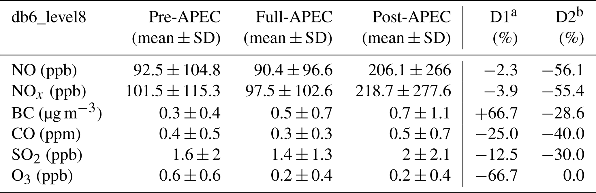
^a D1 = (full-APEC − pre-APEC) ∕ pre-APEC. ^b D2 = (full-APEC − post-APEC) ∕ post-APEC.

Figure 9 The distributions (boxplots) of BC∕CO ratios derived from C_veh. obtained from the WTM for the pre-, full-, and post-APEC periods. The black boxes and whiskers denote the 5th, 25th, 75th, and 95th percentiles. The black horizontal bars indicate median values. The black squares represent mean values. Red boxes indicate observations in the daytime and blue boxes indicate observations in the night-time.

Meanwhile, the emission control policies for cars and trucks were more stringent in the daytime than at night. Table 6 shows the changes in C_veh. during different observation periods and between daytime and night-time. The mean C_veh. of NO, NO_x, BC, and CO during daytime in the full-APEC period were 19.4 %, 17.7 %, 0.0 %, and 50.0 % lower, respectively, than those in the pre-APEC period and were 50.0 %, 47.3 %, 62.5 %, and 50.0 % lower than those in the post-APEC period. The magnitudes of the decreases in C_veh. for daytime NO, NO_x, and BC relative to the pre-APEC period were lower than those relative to the post-APEC period, which confirms that the gradual implementation of control policies during the pre-APEC period had impacts on air quality, as discussed above. The mean C_veh. of NO and NO_x during night-time in the full-APEC period were 65.3 % and 65.4 % lower, respectively, than those in the post-APEC period. The magnitudes of decrease in C_veh. for daytime and night-time of NO, NO_x, and CO in the full-APEC period relative to the post-APEC period were comparable. The magnitude of the decrease in C_veh. for night-time BC in the full-APEC period relative to the post-APEC period was less than that for the daytime, which is related to the differences in vehicle emission control policies between day and night, i.e. the less stringent control policies for trucks (which run on heavy-duty diesel and emit much more BC than cars) for the hours 02:00–06:00 over the entire observation period. As shown in Fig. 9, BC∕CO ratios reflect changes in the fleet profile, i.e. due to the reduced controls on trucks overnight compared with other vehicles during the APEC summit.

Table 6 The mean on-road emission concentrations (i.e. C_veh.) obtained from WTM and their relative changes between the pre-APEC, full-APEC, and post-APEC periods, divided into daytime and night-time.

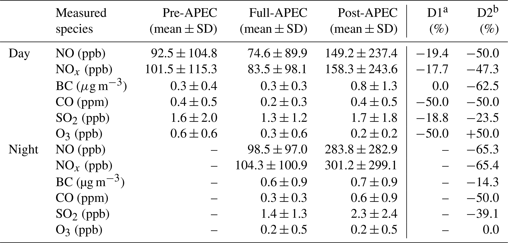
^a D1 = (full-APEC − pre-APEC) ∕ pre-APEC. ^b D2 = (full-APEC − post-APEC) ∕ post-APEC.

4 Conclusions

In this study, we developed and validated a WTM to evaluate the effectiveness of vehicle emission control policies implemented during APEC. The results of the WTM were carefully compared with the MPLM and observations at a ground-based site. These comparisons showed that the WTM is a feasible and stable method for separation of the concentrations contributed by immediate vehicle emissions (C_veh.) and on-road background pollutant concentrations (C_bg.) and can thus be used to evaluate vehicle emission control policies.

The on-road mobile measurements could be used to obtain the temporal and spatial distributions of air pollutants and capture the characteristics of on-road vehicle emissions. The data from on-road measurements around the 4th Ring Road of Beijing from 28 October to 22 November 2014, including the pre-APEC (28 October to 2 November 2014), full-APEC (3–12 November 2014), and post-APEC (13–22 November 2014) periods, were used to conduct a case study.

The C_veh. of NO, NO_x, BC, CO during daytime in the full-APEC period were 19.4 %, 17.7 %, 0.0 %, and 50.0 % lower, respectively, than those in the pre-APEC period and were 50.0 %, 47.3 %, 62.5 %, and 50 % lower than those in the post-APEC period. The C_veh. of NO, NO_x, BC, and CO during night-time in the full-APEC period were 65.3 %, 65.4 %, 14.3 %, and 50.0 % lower than those in the post-APEC period. Overall, our results indicate that the vehicle emission control policies implemented during the full-APEC period were effective. Further exploration of the differences in emission reductions between night-time and daytime suggested that the effectiveness of the vehicle control policies was relatively uniform. However, the less stringent controls on trucks for the hours 02:00–06:00 resulted in less effective abatement of BC emissions, since heavy-duty diesel trucks are an important source of BC (Westerdahl et al., 2009).

However, it should be noted that this study also has some limitations. First, the instrument time resolution was not able to fully capture the instantaneous emission signals during the on-road mobile measurements, especially for BC. Therefore, faster time response air pollution instruments are needed for future studies. Meanwhile, the measurements were only conducted around the 4th Ring Road of Beijing, and thus the results are not fully representative of vehicle emissions in Beijing. Future experiments should include observations for different road conditions and different types of road to enable a more comprehensive study of the contribution of vehicle emissions to air pollution in Beijing. Finally, data on traffic flow and vehicle fleet profiles were lacking, which will be needed to further understand the effectiveness of vehicle emission control policies. We assumed that changes in meteorological conditions were reflected in the low-frequency components and did not influence our evaluation of pollution control polices. The impact of meteorological conditions must be completely eliminated to allow for more accurate assessments of pollution control policies in future studies.