the Creative Commons Attribution 4.0 License.
the Creative Commons Attribution 4.0 License.
 | 30 Oct 2019
The mechanisms and meteorological drivers of the summertime ozone–temperature relationship
Colette L. Heald
Surface ozone (O3) pollution levels are strongly correlated with daytime surface temperatures, especially in highly polluted regions. This correlation is nonlinear and occurs through a variety of temperature-dependent mechanisms related to O3 precursor emissions, lifetimes, and reaction rates, making the reproduction of temperature sensitivities – and the projection of associated human health risks – a complex problem. Here we explore the summertime O3–temperature relationship in the United States and Europe using the chemical transport model GEOS-Chem. We remove the temperature dependence of several mechanisms most frequently cited as causes of the O3–temperature “climate penalty”, including PAN decomposition, soil NOx emissions, biogenic volatile organic compound (VOC) emissions, and dry deposition. We quantify the contribution of each mechanism to the overall correlation between O3 and temperature both individually and collectively. Through this analysis we find that the thermal decomposition of PAN can explain, on average, 20 % of the overall O3–temperature correlation in the United States. The effect is weaker in Europe, explaining 9 % of the overall O3–temperature relationship. The temperature dependence of biogenic emissions contributes 3 % and 9 % of the total O3–temperature correlation in the United States and Europe on average, while temperature-dependent deposition (6 % and 1 %) and soil NOx emissions (10 % and 7 %) also contribute. Even considered collectively these mechanisms explain less than 46 % of the modeled O3–temperature correlation in the United States and 36 % in Europe. We use commonality analysis to demonstrate that covariance with other meteorological phenomena such as stagnancy and humidity can explain the bulk of the remainder of the O3–temperature correlation. Thus, we demonstrate that the statistical correlation between O3 and temperature alone may greatly overestimate the direct impacts of temperature on O3, with implications for the interpretation of policy-relevant metrics such as climate penalty.
- Article
(12394 KB) - Full-text XML
- BibTeX
- EndNote


Tropospheric ozone (O3) negatively influences human health, agricultural crop yields, and ecosystem integrity (Monks et al., 2015; World Health Organization, 2006; Tai et al., 2014; Fuhrer et al., 2016). As a secondary pollutant, O3 is not directly emitted from natural or anthropogenic sources, but rather forms as a result of photochemistry in the presence of precursors including nitrogen oxides (NOx), carbon monoxide (CO), and volatile organic compounds (VOCs). While the chemical processes leading to the formation of tropospheric O3 are well understood, the sensitivity of O3 production to changes in ambient conditions and precursor concentrations is complex and nonlinear. Local NOx and VOC emissions are two of the most important contributors to daytime tropospheric O3 production, but the ratio between the two can be as important as the overall emission magnitudes themselves (Sillman, 1999). NOx∕VOC emission ratios of roughly 1:8 produce the highest O3 production rates in simplified box models (Sillman and He, 2002). Therefore, increases in precursor emissions might increase, maintain, or even reduce O3 concentrations, depending on the initial NOx∕VOC ratio.
Further contributing to this complexity, O3 formation and transport are highly sensitive to local meteorological conditions (Elminir, 2005). Precursor emissions and concentrations themselves can depend on the weather, for example in the case of temperature-dependent emission of biogenic VOCs from vegetation (Guenther et al., 1995). As a product of photochemical reactions, tropospheric O3 formation also requires sunlight, and can be sensitive to atmospheric stability, transport, and mixing conditions. Hot, sunny, stagnant conditions are often associated with the greatest risk of extreme O3 events, as these days typically provide the ideal combination of precursor concentrations, photochemical reactions, and stable conditions for the pollutant to form and persist over an extended period of time (Jacob et al., 1993; Lin et al., 2001).
Because of this sensitivity to climate, increases in continental surface O3 has been identified as a possible negative side effect of a warming climate, a relationship commonly referred to as the “ozone climate penalty”. First coined in 2008 by Wu et al., the climate penalty quantifies the additional ozone present in a warmer environment, as well as the additional anthropogenic emissions reductions necessary to compensate for this enhanced O3 production. Given a 2–5 ppbv increase in O3 expected with 2050 climate projections, Wu et al. (2008) concluded that an additional 10 % reduction in NOx emissions would be necessary to mitigate these climate-driven ozone increases, above and beyond the ongoing reduction in NOx emissions observed across much of the industrialized northern midlatitudes. This climate penalty is highly region-specific, depending on both current local conditions as well as the nature of future changes. In related work, Bloomer et al. (2009) defined the slope of the observed daily O3–temperature correlation as the “climate penalty factor”, and found a decreasing trend in this factor over time as a result of NOx emission reduction efforts.
While not synonymous, the long-term climate penalty defined by Wu et al. (2018) and the daily climate penalty factor calculated by Bloomer et al. (2009) can be understood to be driven by a similar set of temperature-dependent mechanisms. Previous work has examined this temperature–O3 relationship and identified several mechanisms most likely to be responsible, in particular temperature-dependent biogenic VOC emissions and PAN dissociation rates (Jacob et al., 1993; Sillman and Samson, 1995; Jacob and Winner, 2009). Additionally, the temperature dependence of natural soil NOx emissions (Yienger and Levy, 1995) and O3 dry deposition (Wesely, 1989) have been recognized in previous studies, and could contribute to the overall O3–temperature correlation. Each of these four mechanisms is included in typical chemical transport models (CTMs) used to study atmospheric chemistry, making these models useful tools for estimating the relative contributions of each mechanism to the overall O3–temperature relationship.
To investigate the relative importance of each temperature-dependent mechanism in governing the overall O3–temperature relationship we explore multiple regional sensitivity cases with the chemical transport model GEOS-Chem v9-02 (http://www.geos-chem.org, last access: 7 August 2018). GEOS-Chem is driven by assimilated meteorology from the NASA Global Modeling and Assimilation Office (GMAO); here we use the GEOS-5 product for 2010–2011. Our simulations over North America and Europe are performed at the native grid horizontal resolution of with 47 vertical levels. Boundary conditions are provided from a global GEOS-Chem simulation at horizontal resolution.
The default tropospheric chemical mechanism in GEOS-Chem v9-02 includes a description of NOx–hydrocarbon–O3–aerosol chemistry with over 120 species which participate in over 400 kinetic and photolytic reactions (Mao et al., 2013). To better capture the temperature dependence of O3 formation as a result of biogenic emissions, we add monoterpene chemistry to the standard GEOS-Chem v9-02 gas-phase mechanism following Fisher et al. (2016), as in Porter et al. (2017). We use the EPA's NEI2005 emissions inventory for anthropogenic emissions over the United States after scaling them up to match NEI2011 national totals for the years 2010 and 2011, then reducing NOx emissions following the recommendations of Travis et al. (2016). European anthropogenic emissions are taken from EMEP inventories (Auvray and Bey, 2005). To represent global biomass burning we use the GFED3 inventory (Mu et al., 2011). NOx emissions from lightning are treated using a modified parameterization first developed by Price and Rind (1992) and further constrained by satellite data (Murray et al., 2012). Soil NOx emissions and biogenic hydrocarbon emissions are calculated online following the Hudman et al. (2012) and MEGAN2.1 (Guenther et al., 2012) schemes. Dry deposition is modeled using the Wesely “resistor in series” approach (1989). Wet removal includes contributions from scavenging in convective updrafts, in-cloud rainout, and below-cloud washout and is described by Amos et al. (2012).
GEOS-Chem has been shown to reproduce key spatiotemporal features of surface and column ozone observations, though biases and uncertainties are also known (Zhang et al., 2011; Hu et al., 2017). In particular, uncertainties in anthropogenic emission inventories (Travis et al., 2016), various drivers of biogenic emissions (Arneth et al., 2011; Vinken et al., 2014), and lightning NOx (Murray, 2016) have been found to play important roles in the variability of tropospheric ozone and its precursors. Uncertainties in spatial inputs, including the datasets used to drive biogenic emissions such as plant functional type and leaf area index distributions, can also influence the resulting biogenic emissions and ozone impacts, and changes or updates to these inputs would influence the magnitude and distribution of the resulting temperature sensitivities (Guenther et al., 2006; Arneth et al., 2011). Ongoing advances in the development of chemical mechanisms relevant to ozone formation and loss (Mao et al., 2013; Sherwen et al., 2016) have also underscored the importance of chemistry. While a full analysis of the sensitivity of the O3–T relationship to each of these factors is beyond the scope of this work, uncertainties in these and other modeled parameters and inputs can all influence both overall ozone production and the temperature sensitivities examined here.
2.1 Ozone–temperature mechanisms in the GEOS-Chem model
The temperature dependence of biogenic VOC emissions (especially those of isoprene) has been frequently cited as an important mechanism contributing to the observed O3–temperature correlation (Wu et al., 2008; Jacob and Winner, 2009; Doherty et al., 2013; Rasmussen et al., 2013), but the magnitude of this biogenic contribution to O3–temperature sensitivity remains uncertain. Additional VOC emissions on hot days would be expected to increase O3 production in areas high in NOx, but other areas – especially those with a particularly low NOx∕VOC ratio – might show constant or even reduced O3 levels due to ozone quenching (Loreto and Velikova, 2001), leading to an inverse relationship. Biogenic emissions also do not necessarily vary linearly with temperature. Isoprene emissions, for example, are observed to plateau and eventually shut down completely at very high temperatures (Harley et al., 1999). Representative isoprene and monoterpene emissions response curves are shown in Fig. 1a, based on the GEOS-Chem implementation of MEGAN2.1. In the United States, isoprene and monoterpene emissions are highest in the southeast region, where high temperatures and foliage density provide ideal conditions in summer months (Fig. 2a and b). Europe is characterized by much lower emissions of isoprene overall, though monoterpene emitters are relatively common across the region (Fig. 2a and b).
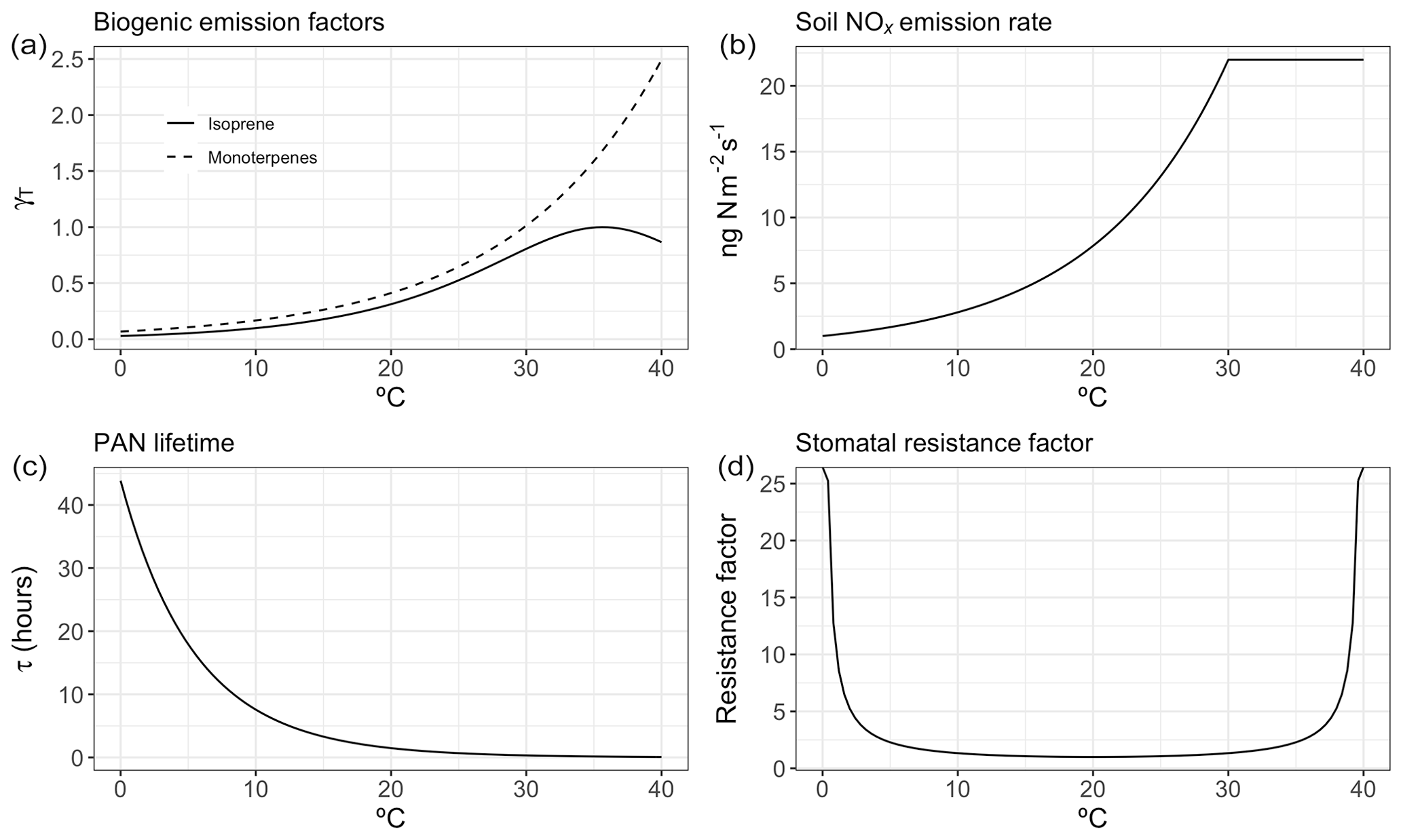
Figure 1Representative temperature-dependent mechanism responses within GEOS-Chem for biogenic emissions (a), soil NOx emissions (b), PAN lifetime (c), and stomatal resistance (d).
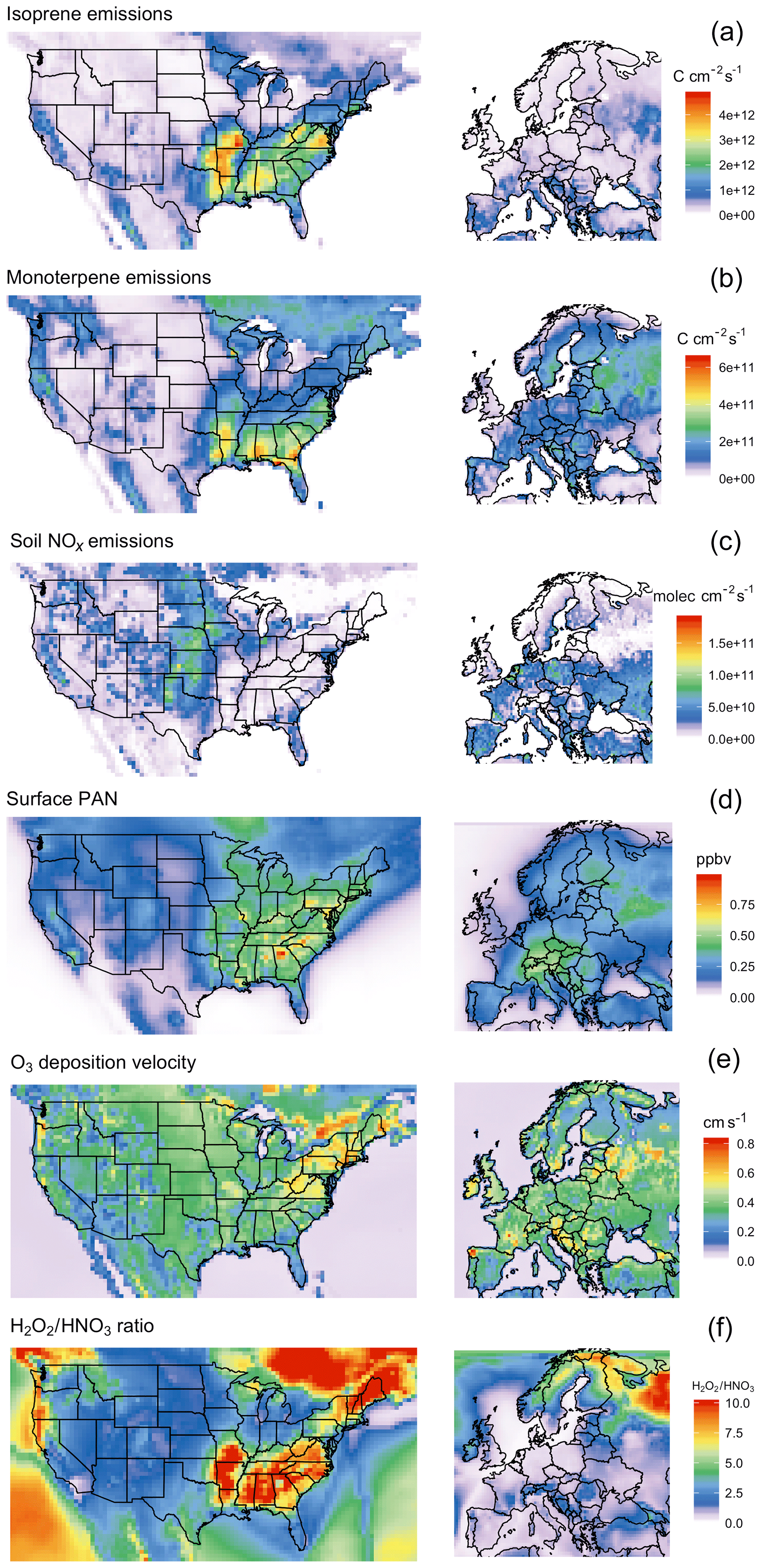
Figure 2Summer mean values (JJA 2010–2011) for modeled isoprene and monoterpene emissions (a, b), soil NOx emissions (c), surface PAN mixing ratios (d), O3 deposition velocity (e), and NOx∕VOC sensitivity as represented by the surface H2O2∕HNO3 ratio (f).
While NOx levels in the lower troposphere are dominated by anthropogenic sources throughout the year, natural processes can also play an important role (Zhang et al., 2003). Of the commonly recognized biogenic sources of NOx, emissions of NO as a result of microbial activity in the soil have the clearest and most widely observed temperature relationship (Williams et al., 1992). Building upon the work of Hudman et al. (2012) and others, GEOS-Chem includes an exponential temperature-dependent factor for soil NOx emissions, with plateaus at 30 ∘C (Fig. 1b), along with additional factors to account for vegetation type, soil moisture, fertilizer treatment, and canopy losses. This scheme has been shown to produce NO2 levels in broad agreement with satellite observations in terms of spatial and temporal variability, though a systematic underprediction in model results suggests that modeled soil emissions may need to be further increased overall (Vinken et al., 2014). Modeled summer NOx emissions vary greatly by location, peaking in the American Midwest and southern European countries (Fig. 2c).
As a so-called NOx reservoir species, PAN (CH3COO2NO2) serves as an important means of nitrogen transport and is one of the primary chemical links between O3 and daytime temperature. A product of reactions between non-methane VOCs and NOx, PAN has an atmospheric lifetime that is typically longer than its ozone-producing precursors. However, due to the temperature dependence of its primary sink – thermal decomposition – this lifetime varies significantly based on meteorological conditions, with warmer temperatures favoring PAN decomposition and thus local NOx production (Fig. 1c and Fischer et al., 2014). This temperature sensitivity has been identified as a dominant reason for the O3–temperature relationship in past measurement and modeling studies (Beine et al., 1997; Dawson et al., 2007; Jacob and Winner, 2009). PAN concentrations tend to correlate with NOx emissions, and therefore modeled concentrations peak in the eastern United States as well as central Europe (Fig. 2d), where anthropogenic emissions are highest.
Depositional loss to vegetation and other surfaces is a key sink of O3 and other pollutants. Traditional models of dry deposition processes use a “resistor-in-series” approach, in which barriers to O3 deposition through various pathways are parameterized and represented as an electrical circuit (Wesely, 1989). This model has had some success in reproducing observed patterns of O3 deposition velocities, though large uncertainties remain due to the scarcity of long-term measurements (Silva and Heald, 2018). In the Wesely resistance scheme, surface temperature influences deposition rates in two ways: through a stomatal resistance term that is very high at two extremes (typically freezing temperatures and around 40 ∘C) and reaches a minimum at some ideal temperature (Fig. 1d), and an exponentially decreasing nonstomatal term designed to reduce deposition over frozen (or nearly frozen) surfaces. In typical summer environments across the United States and Europe, only the stomatal term is relevant in practice, linking extremely high temperatures with increased stomatal resistance, thereby increasing local O3 levels on very hot days. While observations of O3 dry deposition velocities relative to meteorological drivers show mixed results (Clifton et al., 2017), in principle large-scale increases in stomatal resistance as a result of changes in temperature could lead to increases in O3 concentrations. Summer O3 deposition velocities across the United States and Europe as simulated by GEOS-Chem tend to range from 0.2 to 0.5 cm s−1, depending on local surface type and climatology (Fig. 2e).
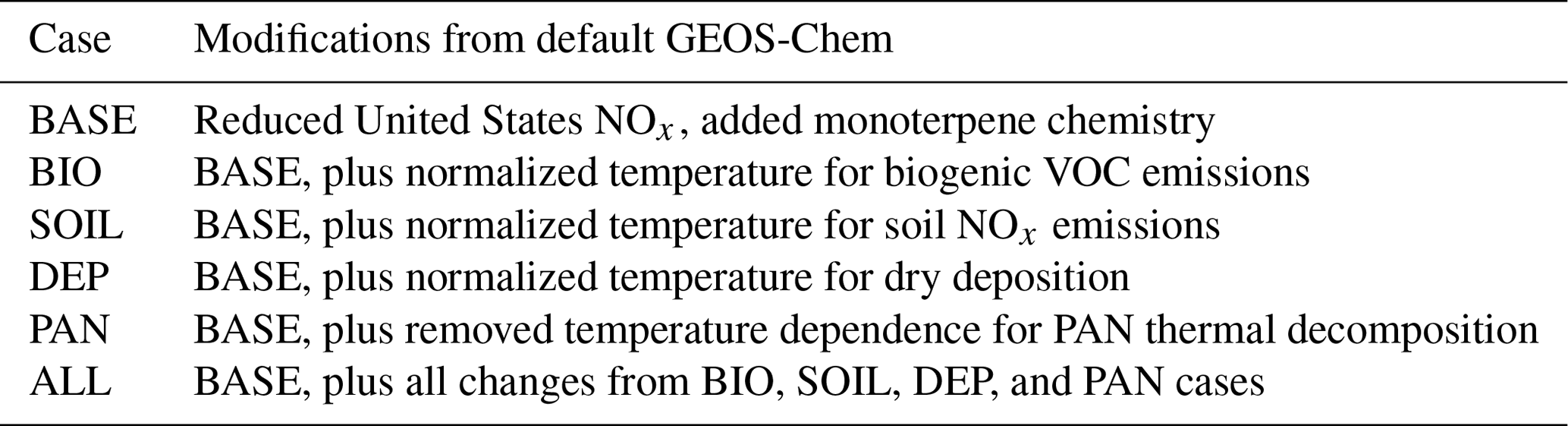
To represent our control case we use a 2-year base scenario (BASE) for 2010–2011 in which temperature-dependent processes within GEOS-Chem are unchanged. We then sequentially remove the temperature dependence from the four key O3–T mechanisms discussed in Sect. 2.1 to explore the impact that each has on the overall O3–T relationship over a 3-month summertime period (JJA), with an additional month for spinup (Table 1). Finally, we run nested regional simulations for each year over the United States and Europe, again discarding the first month of each run to focus on the three summer months (JJA). To isolate the impact of temperature dependence on biogenic emissions (BIO case), dry deposition (DEP case), and soil NOx emissions (SOIL case), we generate a set of hourly temperatures representing the mean summer (JJA) value at each nested grid cell. To do so, we generate mean hourly temperatures for each modeled grid cell by averaging each hour (0 through 23) across the 3 modeled months. This averaged diurnal cycle is then substituted into each examined mechanism in turn, resulting in a repeating temperature profile being applied to calculations related to the modified mechanism. Through this procedure, diurnal patterns are preserved while day-to-day temperature variability for that mechanism is removed, preventing it from directly influencing the overall daily O3–temperature correlation. In the PAN case, the default GEOS-Chem chemical mechanism is modified to remove temperature dependence from PAN dissociation by assuming a local constant temperature of 15 ∘C everywhere for that particular reaction.
To confirm that our four chosen mechanisms (biogenic VOC emissions, soil NOx emissions, PAN dissociation, and dry deposition) are in fact collectively responsible for most of the direct connection between temperature and O3 within GEOS-Chem, we perform an additional set of sensitivity tests over each of our regional domains. In one modified case we uniformly increase all temperatures by 1 ∘C, resulting in widespread increases in average surface O3 levels (Fig. 3a). In a second modified case we again increase temperature by 1 ∘C, but decouple temperature from the four chosen mechanisms using original mean hourly temperatures as described above. In the decoupled case, surface O3 shows negligible differences in mean surface O3 (Fig. 3b and c), indicating that the four decoupled mechanisms dominate the directly modeled O3–T relationship, with the residual O3 changes likely resulting from temperature-dependent chemical kinetics for species other than PAN.
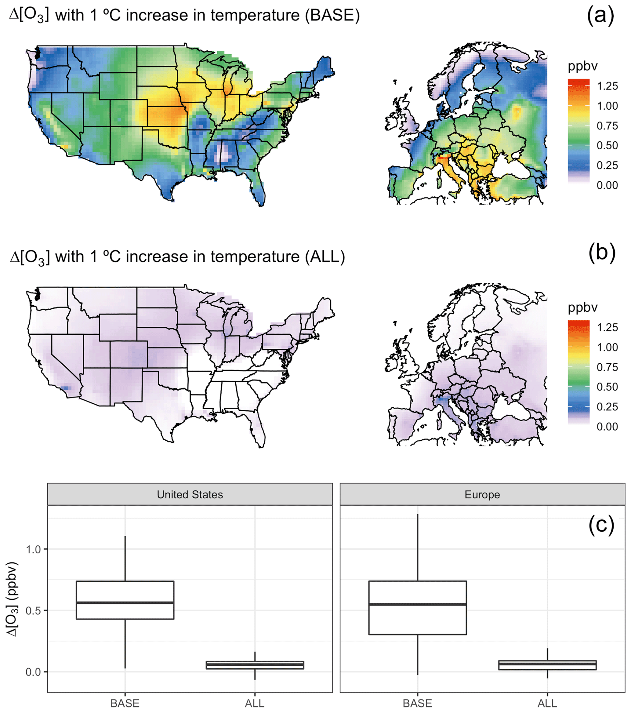
Figure 3Increase in O3 with a 1 ∘C increase in temperature in the BASE case (a) and with fixed temperature mechanisms in the ALL case (b). Distribution of changes for each shown in boxplots (c).
For observational comparison, we use data from the EPA's Air Quality System (AQS) network of monitoring sites (US Environmental Protection Agency, 2016), as well as the AirBase air quality database maintained by the European Environment Agency (EEA).
The simulated O3–temperature relationship in GEOS-Chem for the two modeled summers, as represented by the slope of a gridded O3–T ordinary least-squares (OLS) regression, is fairly consistent with AQS and AirBase observations, lending confidence to the use of modeled sensitivity comparisons to examine the significance of underlying mechanisms (Fig. 4a). In both the United States and Europe, spatial patterns and overall mean values of the O3–T correlation are fairly well represented, though the full range of sensitivities is not reproduced in the model output (root-mean-square error of 0.84 and 0.79, mean bias of 0.02 and −0.13 ppbv O3 ∘C−1 for the United States and Europe respectively). In spite of the relatively strong agreement between modeled and observed O3–T correlations, we highlight a number of shortcomings in the modeled representation of this relationship which may explain the remaining discrepancies between the model and observations. For one, the anthropogenic emission inventories used in GEOS-Chem are independent of daily temperatures, while in reality there are connections between meteorological variability and emissions from human activities such as transportation and energy production. In addition, the grid cell size in GEOS-Chem is incapable of capturing the full diversity of subgrid meteorological phenomena, many of which may be important at the surface station level. Local temperature and O3 fluctuations may vary significantly from those of the gridded average. These issues, among others, may contribute to some of the differences seen in the comparison between observed and modeled sensitivities. In particular, the magnitude of both high and low extremes tends to be underestimated in gridded output from GEOS-Chem, resulting in a tighter distribution of modeled output and skewed slope of modeled vs. observed values, especially in Europe (Fig. 4c). However, in spite of the notable differences between modeled and observed O3–T relationships at the tails of the distributions, a relatively small overall bias is apparent across station types in both urban and remote regions (Fig. 4b). Here, the more remote stations associated with the National Park Service (NPS) are separated from the rest of the AQS dataset for comparison over the United States, while AirBase stations in Europe are split by station area category (urban/suburban and rural). In each category, nearest-neighbor grid cells effectively capture the center of the observed distribution, even though extremes are not fully represented, particularly at rural European stations.

Figure 4Regression slopes of summer (JJA) daily maximum 8 h average O3 vs. daily maximum temperature for GEOS-Chem and station observations in the United States and Europe. Station data points are overlaid on gridded model output in panel (a). Distributions for observed (black) and modeled (red) O3–T slopes are shown in panel (b), further separated by station category: US stations are separated between the more remote NPS stations and the remaining stations of the AQS network, while European stations are split by AirBase area category into urban/suburban and rural station types. Scatterplots in panel (c) show modeled values vs. observed, with green points used to mark NPS stations in the US and rural area stations in Europe. The remaining AQS stations, as well as those AirBase stations categorized as urban or suburban, are shown as black points.
Given that the mean values and spatial distribution of regional O3–T sensitivities are generally consistent with observations, we analyze the mechanisms contributing to modeled sensitivities by decoupling them from temperature variability individually and simultaneously. Removing temperature dependence from the four chosen mechanisms has noticeable impacts on correlations between temperature and O3 in the simulated cases, with regional differences apparent in each case. For each of the four cases examined, the strength of the O3–temperature dependence (measured via the coefficient of determination R2) was examined through linear regression and compared to that seen in the BASE case. When subtracted from the BASE values, the resulting difference in R2 can be understood as the contribution of that particular mechanism to the overall modeled sensitivity (Fig. 5).
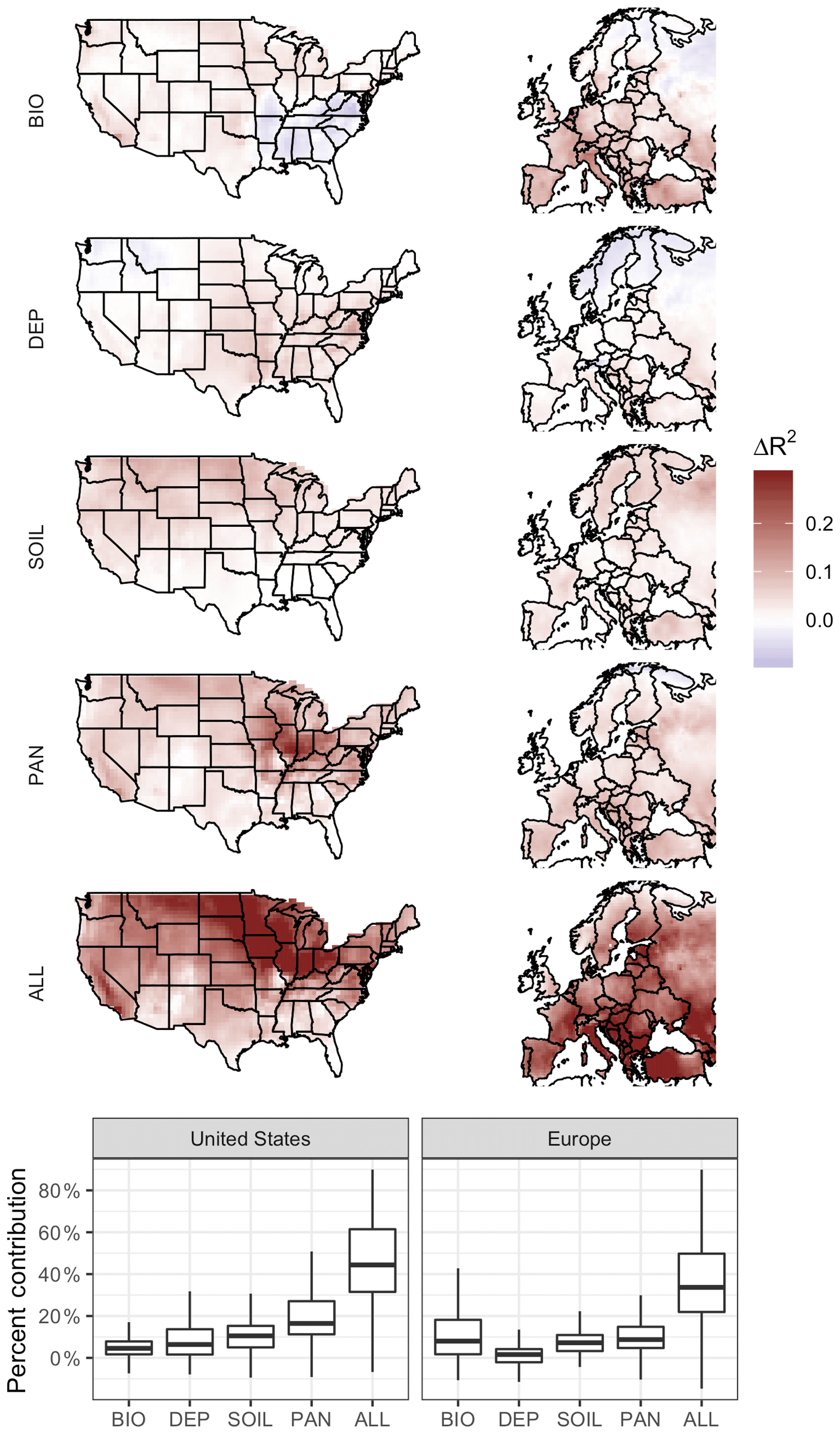
Figure 5Impact of temperature dependence of biogenic emissions, O3 dry deposition, soil NOx emissions, PAN lifetime, and all mechanisms at once. Plotted values show the difference between O3–temperature correlation in the BASE case and that of the modified case in which dependence on daily temperature variability is removed.
Temperature-dependent biogenic VOC emissions have a positive impact on O3–temperature correlation through most of the United States, especially around urban centers, but have a negative impact across much of the southeast. This is consistent with expectations based on NOx∕VOC ratios (Fig. 2f), in which NOx-rich regions experience a boost in O3 production when rising temperatures lead to additional VOC emissions. Much of the southeast region of the United States, however, is already saturated in VOCs (primarily isoprene), and thus additional emissions on hot days reduce O3 production efficiency, or even act as an O3 sink. The heavily forested northern regions of Europe are likewise less influenced (or even negatively influenced) by the temperature dependence of biogenic emissions, while the high-NOx regions of central and southern Europe show strong positive contributions. Changes in R2 reach up to 0.14 and 0.21 in the United States and Europe, respectively, representing on average 3 % and 9 % of the overall regional O3–T correlation (Fig. 5).
The impact of temperature dependence in dry deposition is distributed roughly congruently with leaf area index (LAI) coverage across the United States, contributing up to 0.14 to the O3–T R2 but only 0.02 on average. Little effect is seen in the heavily forested regions of Northern California and the Pacific Northwest, but since deposition is a removal effect and O3 levels are relatively low in those regions to begin with, changes in deposition rates could be expected to have minimal impact on the overall O3–temperature relationship there. Relative contributions of deposition on a local basis, however, can represent over one-quarter of the overall O3–T correlation in some US locations. The overall impact of temperature-dependent dry deposition is even less pronounced in Europe, reaching up to 0.08, but averaging less than 0.01 across the region.
Temperature-dependent soil NOx emissions contribute around 0.04 to the coefficient of determination in both regions, representing 10 % of the total R2 value in the United States and 7 % in Europe. Notably, the impact of temperature dependence in soil emissions does not match up directly with the overall magnitude of those emissions themselves (Fig. 2c), indicating that this fluctuation represents a relatively minor and diffuse effect. Areas characterized by lower NOx∕VOC ratios due in part to low NOx emissions (Fig. 2f) are also more likely to exhibit stronger sensitivity to temperature-driven soil NOx variability.
The temperature dependence of PAN decomposition is a strong contributor to the O3–temperature relationship in both the United States and Europe, particularly in the American Midwest, where the positive impact of this mechanism reaches 0.32. Impacts are also visible across most of the eastern United States, as well as the Southern California and Central Valley regions, and the O3–T R2 increases by 0.07 on average in the US (almost 20 % of the total mean). PAN temperature sensitivity is also a strong contributor to the O3–T relationship in Europe by up to 0.14 (9 % of total mean R2). Of the examined model mechanisms in the United States, PAN lifetime is the strongest overall contributor to the correlation between O3 and temperature, though it places a close second to biogenic emissions in Europe.
While each modeled mechanism contributes to the overall O3–T relationship in the United States and Europe, none of them come close to completely explaining the BASE case correlation between O3 and T. Even when all temperature-dependent mechanisms are removed from the model (the ALL case), most regions still show O3–temperature sensitivities of 50 % or more of their original BASE values as measured by R2. While there are uncertainties associated with comparing statistical sensitivities across these simulated cases, it seems clear that the O3–temperature relationship cannot be fully (or even mostly) explained by these four mechanisms within GEOS-Chem (Fig. 5).
Beyond the directly temperature-dependent emission and loss mechanisms examined within GEOS-Chem, many other meteorological effects can influence surface O3 levels, and correlations between these phenomena and temperature could show up as part of the observed O3–temperature correlation. For example, strong winds can act as a removal mechanism for locally produced O3. If strong winds are also correlated to cooler temperatures, this would show up as a positive correlation between O3 and temperature, despite the lack of any explicit temperature-dependent mechanism. While decoupling other meteorological processes from temperature in the manner demonstrated above can be highly problematic, even within a model, statistical methodologies such as commonality analysis allow for some degree of attribution of observed predictive power between temperature and the other meteorological drivers (Seibold and McPhee, 1979). Derived from the analysis of linear regression output, commonality analysis involves the calculation of R2 values for all possible permutations of predictor variables included in the analysis. These R2 values are then compared, allowing for the calculation of explained variability that is uniquely provided by one variable or another, along with explained variability that is shared between two or more of the covariates. For the purposes of this study, “unique” refers to that portion of a variable's correlation with the response variable (ozone) that is not shared with any other predictor, while “shared” refers to the portion of the correlation that could be attributed to multiple predictors. A more detailed explanation of the equations involved, as well as examples of their application, can be found in Seibold and McPhee (1979).
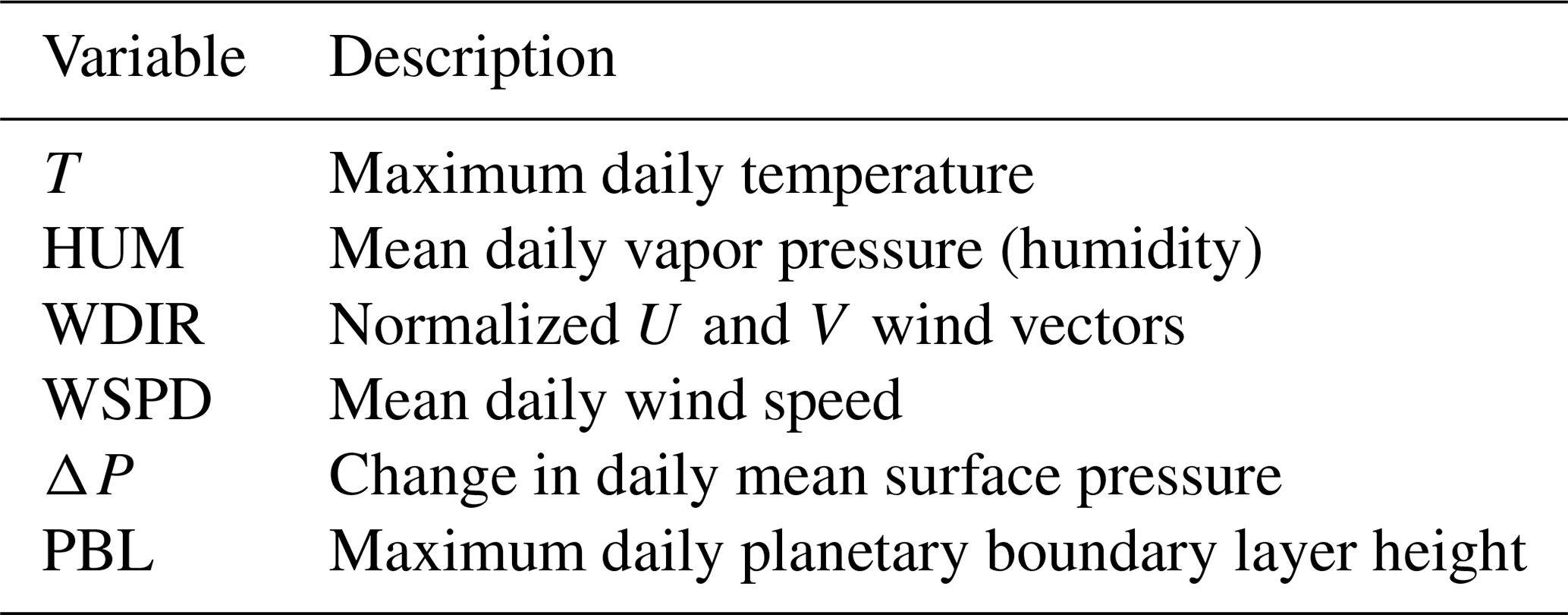
To quantify the contributions of meteorological variables to the modeled O3–temperature correlation, we apply commonality analysis to all gridded output. Through this methodology we are able to decompose all gridded surface O3–temperature R2 values into unique and shared contributions among each of the five variables examined, which are summarized in Table 2: maximum daily temperature (T), humidity (HUM, represented by dew point temperature), mean wind speed (WSPD), wind direction (WDIR), change in mean surface pressure (ΔP), and planetary boundary layer (PBL) height. The unique correlations for each of these variables are shown in Fig. 6, along with the portion of their correlation shared with any other variables (in the case of T) or shared with daily maximum temperature (in the case of the other five meteorological variables).
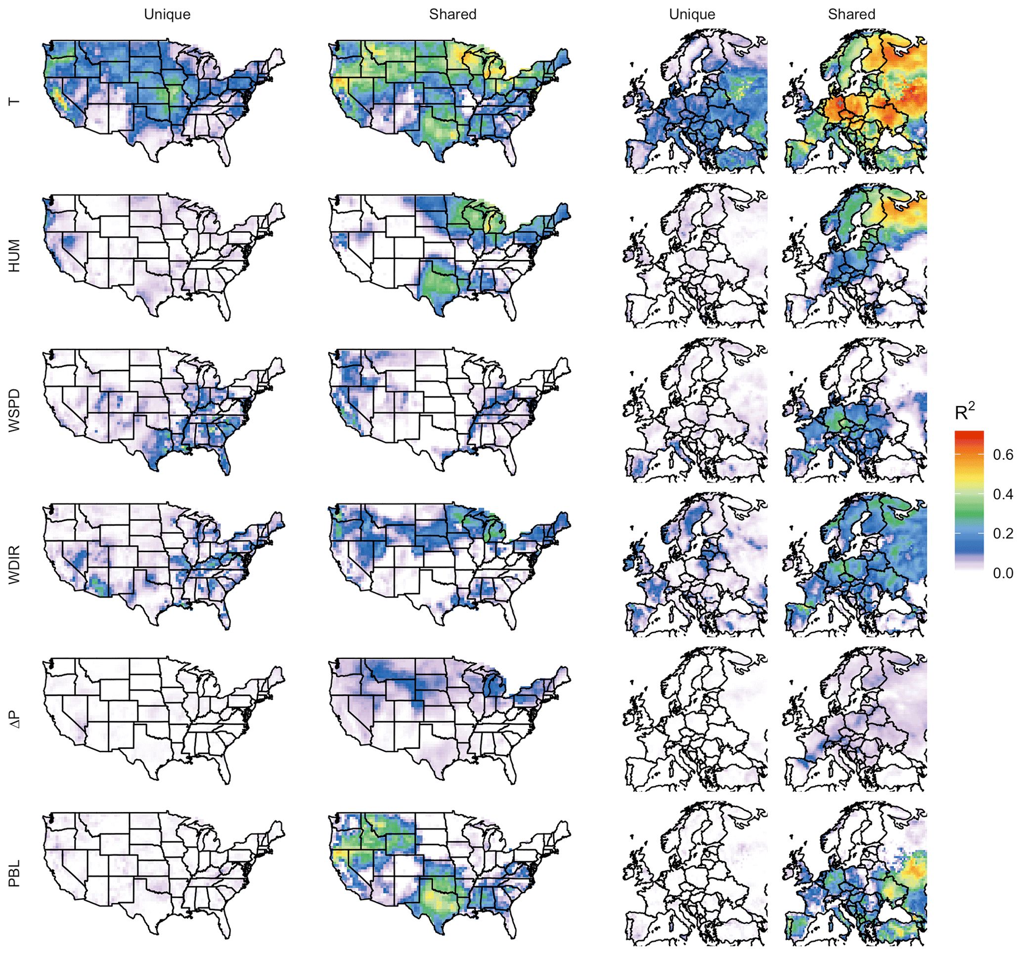
Figure 6Unique and shared O3 correlation among meteorological variables in the BASE case. Unique contributions represent predictive power provided by one meteorological covariate alone, while shared correlation could be attributed to one or more other covariates.
Each unique component represents the portion of explained variability that could be explained solely by one meteorological variable among the six, meaning that the R2 value would be expected to drop by that amount if the predictor were removed from the linear fitting equation. Shared components can be understood as overlap between predictor variable contributions, meaning that the actual mechanism responsible for the correlation might reasonably be attributed to any of the involved predictors. While this methodology is imperfect, especially given the assumption that not all relevant meteorological processes are represented by these six predictors, it does provide additional insight into how and where the O3–temperature correlation might be at least partially explained by correlation with other meteorological phenomena.
As shown, temperature has the strongest and most widespread unique correlation with O3 variability of any of the six meteorological variables included in both the United States and Europe. However, even this strong unique contribution is significantly less than the magnitude of the shared component, meaning that collectively the remaining five predictors could potentially explain the majority of the predictive power that temperature offers alone. The overall predictive power for each meteorological variable, along with the respective shared and unique components, can be further visualized through their mean values across all grid cells. Figure 7 shows region-averaged attribution of shared and unique correlation through stacked columns: each individual column height shows the total correlation (in the form of R2) between ozone and a single meteorological variable, while individually shaded sections differentiate unique and shared components. In each meteorological column that particular variable's unique contribution is at the bottom, and shared contributions are grouped where possible into clusters of two or three total variables for clarity. To best represent the unique contribution of temperature, commonality analysis presented here is performed on the ALL case, with all four chosen temperature-dependent mechanisms decoupled. The difference in total correlation between ALL and BASE cases (which are driven by identical meteorology) is then added into the unique temperature contribution, as this gap can be fully attributed to temperature dependence. Therefore, performing commonality analysis on the BASE case alone would underpredict the unique temperature contribution since some percentage of variability driven specifically by temperature-dependent mechanisms could also correlate with other meteorological variables. Combining commonality analysis along with the results of the BASE-ALL comparison makes full use of the attribution information contained in each since any lost correlation with temperature-dependent mechanisms turned off can be attributed directly to temperature alone, better constraining the commonality analysis itself. Through this analysis it is apparent that over half of the O3–temperature relationship in the United States and Europe (shown by the leftmost bar in each panel) can be explained through correlation with one or more meteorological covariates, especially wind direction, humidity, and planetary boundary layer height. Europe shows an even stronger overall correlation between temperature and O3, and much of that increase appears to be related to a stronger influence from wind and humidity.
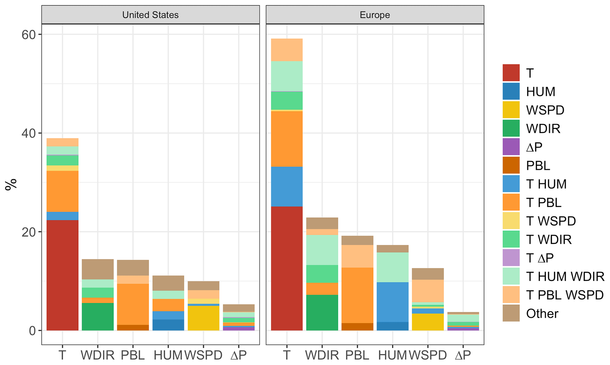
Figure 7Unique and shared contributions to O3 correlation for each of six different meteorological variables in the BASE case. Column heights represent overall predictive power for each variable, while individual colors indicate predictive power unique to that variable (bottom color in each column) or shared by one or more other meteorological variables.
We note that these unique and shared designations are heavily dependent on predictor variable choice and would certainly vary when calculated using a different set of meteorological predictor variables. Uniqueness in these figures should, therefore, be taken as an upper limit estimate, as the inclusion of additional meteorological covariates could demonstrate commonality with temperature where this six-variable set does not. Furthermore, commonality shared between meteorological variables does not imply causation by any one of the members – it only indicates shared statistical predictive power and the possibility of alternative O3-producing mechanisms. However, there are a number of possible mechanisms that could explain some of the predictive power demonstrated by non-temperature variables. Wind speed and direction have perhaps the most straightforward meteorological relationship to O3, and they represent transport of the pollutant either to or away from its source location. Wind speed is generally inversely correlated to high temperatures, and stable conditions are also favorable for the buildup and retention of high O3 concentrations. Depending on local topography and pressure patterns, wind direction can also correlate strongly with changes in temperature, shifting the final destination of polluted air masses from one location to another. Previous work described a relatively small role for these advective mechanisms (Camalier et al., 2007), but the results here suggest that, after temperature-specific mechanisms have been accounted for, wind speed and direction together account for a larger fraction of explained O3 variance than previously suggested. Humidity can influence O3 formation in a number of ways, both directly and indirectly. Water vapor itself participates in competing O3-related effects: water molecules act as O3 sinks by reacting with O(1D) atoms to produce OH, preventing the excited oxygen from re-generating O3. However, in polluted conditions the OH can then act as an O3 precursor itself, potentially increasing production through reactions with CO and VOCs. These competing effects may explain the relatively weak unique contribution of humidity on average, though the high shared fraction (especially in Europe) suggests that other indirect impacts may be involved, such as correlation with cloud cover or fog. Mixing depth has shown mixed results as a predictor for ozone in past studies as well (Jacob and Winner, 2009), as the impact of PBL variability depends strongly on location and local conditions. Areas with low surface O3 can show positive correlations with mixing layer height due to the entrainment of higher concentrations from aloft, while polluted regimes can show strongly negative correlations due to the higher concentrations of trapped precursors on low-PBL days.
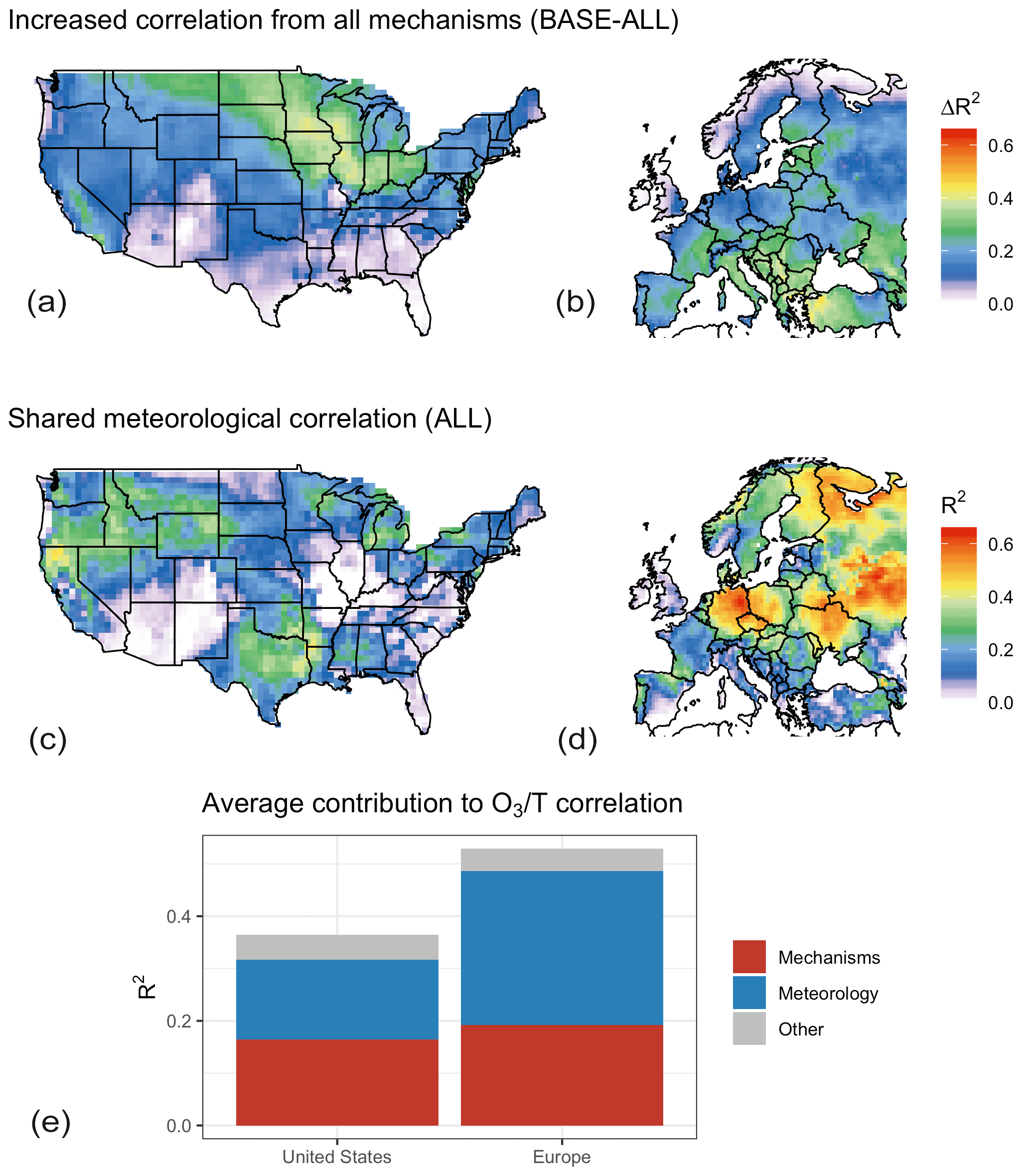
Figure 8Total contribution of modeled mechanisms to the O3–temperature correlation in GEOS-Chem (a, b), possible contribution of the other included meteorological variables (c, d), and mean value for each category by region as a fraction of the total O3–temperature correlation (e, f).
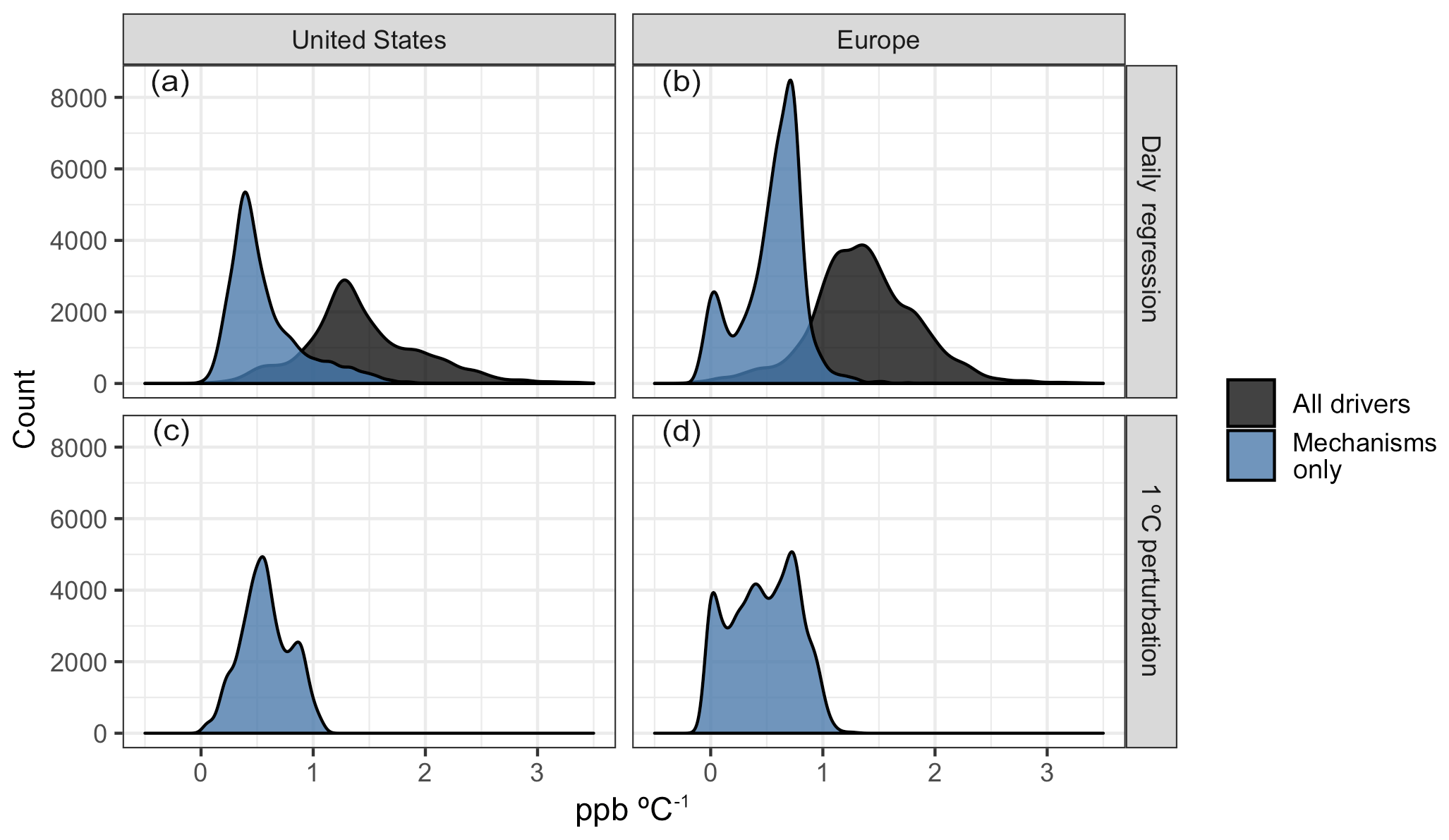
Figure 9Distribution of O3–T sensitivities as measured by the slope of OLS regression (above) and mean surface O3 differences from a flat 1 ∘C temperature perturbation (below). Regression values are shown for all modeled drivers (BASE case, black) and the portion of those slopes attributable to temperature-dependent mechanisms (BASE − ALL, blue).
Although the specific mechanisms through which the non-temperature meteorological variables impact O3 are not identified through this statistical methodology, it is apparent that the majority of modeled O3–temperature correlation left unexplained with the decoupling of temperature-dependent mechanisms (T–O3 R2 in the ALL case, Fig. 5) can itself be explained in principle through covariance with other meteorological variables, indicating that this covariance could explain the residual correlation left over when temperature-dependent mechanisms are turned off within GEOS-Chem. While the difference in O3–T correlation between the BASE and ALL cases shows that these temperature-dependent mechanisms do indeed strongly influence the O3–temperature correlation across a large portion of the northern United States and southern Europe (Fig. 8a, b), the remaining correlation makes up the larger overall fraction. Shared explanatory power, as indicated by the shared contribution of temperature in the ALL case (Fig. 8c, d), indicates that covariance with one or more additional meteorological variables could explain most of the remaining O3–T correlation (Fig. 8e). In this panel, red areas of each column represent the fraction of BASE O3–T correlation that is lost through the decoupling of temperature-dependent mechanisms, blue areas show the shared fraction of remaining temperature dependence in the ALL case, and the gray region represents remaining O3 variability that is uniquely explained by temperature but unaffected by the four described mechanisms. This remaining correlation could be the result of imperfectly chosen meteorological variables, residual temperature dependence within the model from chemistry or other mechanisms, or other fluctuations in emissions or other inputs that happen to covary with temperature.
While day-to-day O3–temperature variability is a useful and commonly examined metric for estimating future changes in air quality under a warming climate, it presents challenges with respect to the extrapolation of daily variability into long-term trends. For example, areas that exhibit little day-to-day variability in summer temperature over the study period may appear to be insensitive to climate change, even though the low O3–temperature correlation is simply a result of short-term climatological stability. The temperature perturbation cases described previously and shown in Fig. 3a provide some additional information on how the daily sensitivities examined here compare to larger, long-term shifts. Figure 9a, b show the distribution of O3–T sensitivities, both as a whole (black fill) and considering only the four key mechanisms previously examined (blue fill). These distributions can then be compared to the distribution of O3 changes apparent with a simple temperature perturbation (panels c and d), which intrinsically includes no other meteorological covariance. While the day-to-day correlation between O3 and temperature from all modeled drivers (Fig. 9a, b, black fill) predicts increases in O3 of around 1.4 ppb for a 1 ∘C increase in temperature, roughly half of that is attributable to the examined mechanisms alone. This portion attributed to mechanisms alone is consistent with the mean change in O3 observed from a 1 ∘C increase in temperature (0.58 ppb in the US and 0.47 ppb in Europe). Together, the consistency of these two outcomes indicates that projections of O3 concentrations under future climate scenarios will be dependent on an accurate representation of temperature-dependent meteorology and dynamics and that models relying on temperature-dependent emissions and chemical mechanisms alone may underpredict the strength of O3–T sensitivities by over 60 %.
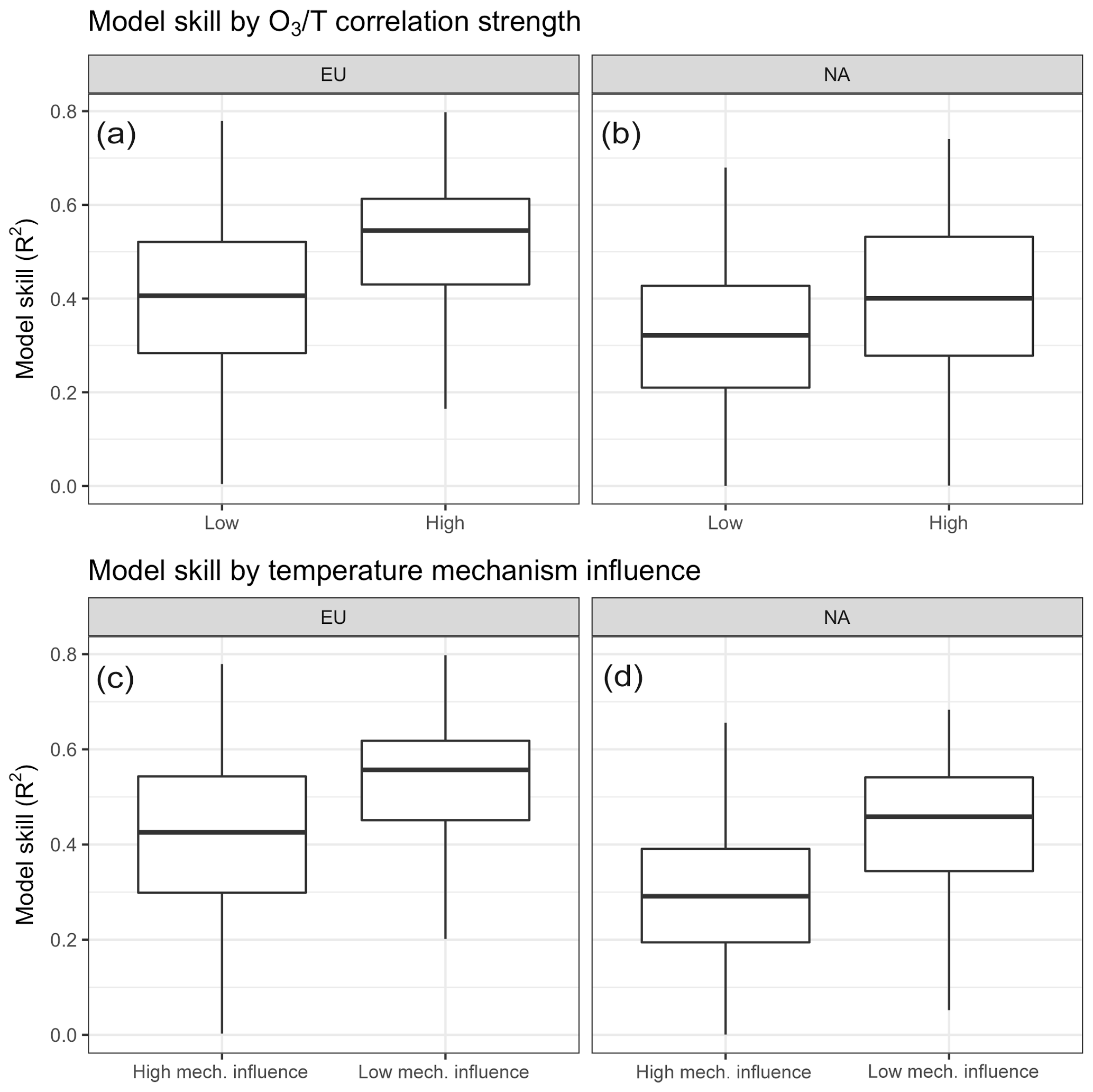
Figure 10Differences in model skill compared to surface station observations as a function of overall O3–temperature correlation (a, b) and the relative importance of modeled temperature-dependent mechanisms (c, d).
Model behavior can be further analyzed through comparison to surface station observations, which reveals a significant difference (P<0.001) in model skill (as measured by modeled vs. observed daily mean O3) when grouping stations by overall O3–T correlation as well as by the relative importance of modeled mechanisms (Fig. 10). Matching observations from the EPA's AQS network in the United States and the EEA's AirBase dataset for Europe with nearest-neighbor grid cells from GEOS-Chem output shows that model skill tends to be higher in regions characterized with above-average O3–temperature correlation (BASE case O3–temperature R2>0.42). While this does not imply that temperature-dependent processes are all modeled correctly, it does at least suggest that temperature-based drivers tend to be better captured by the model than other influences on O3 variability. However, splitting observed stations based on the relative importance of internally modeled mechanisms shows that more work may need to be done on these implementations. Grid cells in which the modeled O3–temperature relationship was dominated by temperature-dependent mechanisms (greater than 50 % of the O3–temperature correlation lost when temperature dependence was removed in the ALL case) showed much less overall predictive power when compared to the corresponding surface observations (Fig. 10c, d).
A changing climate implies changes in the physical and chemical regimes governing the emission, formation, and transport of pollutants such as tropospheric O3. Previous work has identified increasing temperatures in particular as a driver of elevated surface O3 concentrations, mitigating the effectiveness of ongoing emissions reductions in the United States and Europe. This means that, under a warming climate, polluted regions would need to cut emissions even further to achieve the same improvement in air quality, adding economic and human health costs to the bottom line of climate change adaptation. Understanding the mechanisms driving the observed relationship between O3 and temperature is important for guiding improvements in model performance, as well as for better understanding the effects of future changes.
We show here that while temperature-dependent mechanisms such as biogenic emissions and PAN dissociation are often cited as key contributors to the observed O3–temperature relationship, model simulations maintain strong O3–temperature correlations even when these mechanisms are completely decoupled from temperature variability. Analysis of other meteorological variables suggests that meteorological covariance with temperature may explain a large proportion of O3–temperature correlation – over 40 % in the United States and nearly 60 % in Europe. The relative importance of covarying atmospheric dynamics indicates that simulations investigating temperature perturbations alone will underestimate overall O3 impacts by a factor of 2 or more, unless temperature-driven changes in other meteorological patterns are also included and accurately represented. Furthermore, comparison with station observations shows that modeled daily O3 values are less skillful in areas where the O3–temperature correlation is dominated by modeled temperature-dependent mechanisms rather than meteorology, indicating that improved representation of these mechanisms in particular may improve overall model skill with respect to O3 modeling and forecasting.
These results highlight the complexity of pollution projections under changing emissions and climatological conditions, as well as with the attribution of those changes to any individual driver or metric. While surface temperatures can be easily linked to O3 variability statistically, it is apparent that the robustness of this relationship depends on how consistently coupled those temperature changes continue to be, not only with temperature-dependent physical and chemical drivers of O3 formation, but also with the covarying meteorological patterns that appear to be just as influential. These relationships are further confounded by ongoing changes in anthropogenic emissions, making it especially important to understand the ways in which policy-driven emissions reductions may improve – or fail to improve – air quality within a changing climate. Ongoing investigations into the importance of these mechanisms, emissions, and atmospheric dynamics will guide future model development, improving forecast skill and better informing policy decision-making.
GEOS-Chem code is available at http://acmg.seas.harvard.edu/geos/ (last access: 1 March 2018). Data from the EPA's AQS network of surface air quality observations are available at https://www.epa.gov/aqs (last access: 9 August 2016), while AirBase data maintained by the EEA are available at https://www.eea.europa.eu/data-and-maps/data/airbase-the-european-air-quality-database-7 (last access: 31 July 2015).
Development of the ideas and concepts behind this work was performed by both authors. Model execution, data analysis, and paper preparation were performed by WCP with feedback and advice from CLH.
The authors declare that they have no conflict of interest.
This work was supported by the EPA STAR program (RD-83522801) and a core center grant from the National Institute of Environmental Health Sciences, National Institutes of Health (P30-ES002109). Although the research described in this article has been funded in part by the US EPA through grant/cooperative agreement, it has not been subjected to the agency's required peer and policy review and therefore does not necessarily reflect the views of the agency and no official endorsement should be inferred. The authors acknowledge Brian J. Reich for useful discussions.
This research has been supported by EPA STAR (grant no. RD-83522801) and the NIH (grant no. P30-ES002109).
This paper was edited by Federico Fierli and reviewed by two anonymous referees.
Amos, H. M., Jacob, D. J., Holmes, C. D., Fisher, J. A., Wang, Q., Yantosca, R. M., Corbitt, E. S., Galarneau, E., Rutter, A. P., Gustin, M. S., Steffen, A., Schauer, J. J., Graydon, J. A., Louis, V. L. St., Talbot, R. W., Edgerton, E. S., Zhang, Y., and Sunderland, E. M.: Gas-particle partitioning of atmospheric Hg(II) and its effect on global mercury deposition, Atmos. Chem. Phys., 12, 591–603, https://doi.org/10.5194/acp-12-591-2012, 2012.
Arneth, A., Schurgers, G., Lathiere, J., Duhl, T., Beerling, D. J., Hewitt, C. N., Martin, M., and Guenther, A.: Global terrestrial isoprene emission models: sensitivity to variability in climate and vegetation, Atmos. Chem. Phys., 11, 8037–8052, https://doi.org/10.5194/acp-11-8037-2011, 2011.
Auvray, M. and Bey, I.: Long-range transport to Europe: Seasonal variations and implications for the European ozone budget, J. Geophys. Res.-Atmos., 110, D11303, https://doi.org/10.1029/2004JD005503, 2005.
Beine, H. J., Jaffe, D. A, Herring, J. A, Kelley, J. A, Krognes, T., and Stordal, F.: High-Latitude Springtime Photochemistry. Part I: NOx, PAN and Ozone Relationships, J. Atmos. Chem., 27, 127–153, https://doi.org/10.1023/A:1005869900567, 1997.
Bloomer, B. J., Stehr, J. W., Piety, C. A., Salawitch, R. J., and Dickerson, R. R.: Observed relationships of ozone air pollution with temperature and emissions, Geophys. Res. Lett., 36, L09803, https://doi.org/10.1029/2009GL037308, 2009.
Camalier, L., Cox, W., and Dolwick, P.: The effects of meteorology on ozone in urban areas and their use in assessing ozone trends, Atmos. Environ., 41, 7127–7137, https://doi.org/10.1016/j.atmosenv.2007.04.061, 2007.
Clifton, O. E., Fiore, A. M., Munger, J. W., Malyshev, S., Horowitz, L. W., Shevliakova, E., Paulot, F., Murray, L. T., and Griffin, K. L.: Interannual variability in ozone removal by a temperate deciduous forest, Geophys. Res. Lett., 44, 542–552, https://doi.org/10.1002/2016GL070923, 2017.
Dawson, J. P., Adams, P. J., and Pandis, S. N.: Sensitivity of PM2.5 to climate in the Eastern US: a modeling case study, Atmos. Chem. Phys., 7, 4295–4309, https://doi.org/10.5194/acp-7-4295-2007, 2007.
Doherty, R. M., Wild, O., Shindell, D. T., Zeng, G., MacKenzie, I. A., Collins, W. J., Fiore, A. M., Stevenson, D. S., Dentener, F. J., Schultz, M. G., Hess, P., Derwent, R. G., and Keating, T. J.: Impacts of climate change on surface ozone and intercontinental ozone pollution: A multi-model study, J. Geophys. Res.-Atmos., 118, 3744–3763, https://doi.org/10.1002/jgrd.50266, 2013.
Elminir, H. K.: Dependence of urban air pollutants on meteorology, Sci. Total Environ., 350, 225–237, https://doi.org/10.1016/j.scitotenv.2005.01.043, 2005.
Fischer, E. V., Jacob, D. J., Yantosca, R. M., Sulprizio, M. P., Millet, D. B., Mao, J., Paulot, F., Singh, H. B., Roiger, A., Ries, L., Talbot, R. W., Dzepina, K., and Pandey Deolal, S.: Atmospheric peroxyacetyl nitrate (PAN): a global budget and source attribution, Atmos. Chem. Phys., 14, 2679–2698, https://doi.org/10.5194/acp-14-2679-2014, 2014.
Fisher, J. A., Jacob, D. J., Travis, K. R., Kim, P. S., Marais, E. A., Chan Miller, C., Yu, K., Zhu, L., Yantosca, R. M., Sulprizio, M. P., Mao, J., Wennberg, P. O., Crounse, J. D., Teng, A. P., Nguyen, T. B., St. Clair, J. M., Cohen, R. C., Romer, P., Nault, B. A., Wooldridge, P. J., Jimenez, J. L., Campuzano-Jost, P., Day, D. A., Hu, W., Shepson, P. B., Xiong, F., Blake, D. R., Goldstein, A. H., Misztal, P. K., Hanisco, T. F., Wolfe, G. M., Ryerson, T. B., Wisthaler, A., and Mikoviny, T.: Organic nitrate chemistry and its implications for nitrogen budgets in an isoprene- and monoterpene-rich atmosphere: constraints from aircraft (SEAC4RS) and ground-based (SOAS) observations in the Southeast US, Atmos. Chem. Phys., 16, 5969–5991, https://doi.org/10.5194/acp-16-5969-2016, 2016.
Fuhrer, J., Martin, M. V., Mills, G., Heald, C. L., Harmens, H., Hayes, F., Sharps, K., Bender, J., and Ashmore, M. R.: Current and future ozone risks to global terrestrial biodiversity and ecosystem processes, Ecol. Evol., 6, 8785–8799, https://doi.org/10.1002/ece3.2568, 2016.
Guenther, A., Hewitt, C. N., Erickson, D., Fall, R., Geron, C., Graedel, T., Harley, P., Klinger, L., Lerdau, M., Mckay, W. A., Pierce, T., Scholes, B., Steinbrecher, R., Tallamraju, R., Taylor, J., and Zimmerman, P.: A global model of natural volatile organic compound emissions, J. Geophys. Res., 100, 8873–8892, https://doi.org/10.1029/94JD02950, 1995.
Guenther, A., Karl, T., Harley, P., Wiedinmyer, C., Palmer, P. I., and Geron, C.: Estimates of global terrestrial isoprene emissions using MEGAN (Model of Emissions of Gases and Aerosols from Nature), Atmos. Chem. Phys., 6, 3181–3210, https://doi.org/10.5194/acp-6-3181-2006, 2006.
Guenther, A. B., Jiang, X., Heald, C. L., Sakulyanontvittaya, T., Duhl, T., Emmons, L. K., and Wang, X.: The Model of Emissions of Gases and Aerosols from Nature version 2.1 (MEGAN2.1): an extended and updated framework for modeling biogenic emissions, Geosci. Model Dev., 5, 1471–1492, https://doi.org/10.5194/gmd-5-1471-2012, 2012.
Harley, P. C., Monson, R. K., and Lerdau, M. T.: Ecological and evolutionary aspects of isoprene emission from plants, Oecologia, 118, 109–123, https://doi.org/10.1007/s004420050709, 1999.
Hu, L., Jacob, D. J., Liu, X., Zhang, Y., Zhang, L., Kim, P. S., Sulprizio, M. P., and Yantosca, R. M.: Global budget of tropospheric ozone: Evaluating recent model advances with satellite (OMI), aircraft (IAGOS), and ozonesonde observations, Atmos. Environ., 167, 323–334, https://doi.org/10.1016/j.atmosenv.2017.08.036, 2017.
Hudman, R. C., Moore, N. E., Mebust, A. K., Martin, R. V., Russell, A. R., Valin, L. C., and Cohen, R. C.: Steps towards a mechanistic model of global soil nitric oxide emissions: implementation and space based-constraints, Atmos. Chem. Phys., 12, 7779–7795, https://doi.org/10.5194/acp-12-7779-2012, 2012.
Jacob, D. J. and Winner, D. A.: Effect of climate change on air quality, Atmos. Environ., 43, 51–63, https://doi.org/10.1016/j.atmosenv.2008.09.051, 2009.
Jacob, D. J., Logan, J. A., Gardner, G. M., Yevich, R. M., Spivakovsky, C. M., Wofsy, S. C., Sillman, S., and Prather, M. J.: Factors regulating ozone over the United States and its export to the global atmosphere, J. Geophys. Res.-Atmos., 98, 14817–14826, https://doi.org/10.1029/98JD01224, 1993.
Lin, C.-Y. C., Jacob, D. J., and Fiore, A. M.: Trends in exceedances of the ozone air quality standard in the continental United States, 1980–1998, Atmos. Environ., 35, 3217–3228, 2001.
Loreto, F. and Velikova, V.: Isoprene Produced by Leaves Protects the Photosynthetic Apparatus against Ozone Damage, Quenches Ozone Products, and Reduces Lipid Peroxidation of Cellular Membranes, Plant Physiol., 127, 1781–1787, https://doi.org/10.1104/pp.010497, 2001.
Mao, J., Paulot, F., Jacob, D. J., Cohen, R. C., Crounse, J. D., Wennberg, P. O., Keller, C. A., Hudman, R. C., Barkley, M. P., and Horowitz, L. W.: Ozone and organic nitrates over the eastern United States: Sensitivity to isoprene chemistry, J. Geophys. Res.-Atmos., 118, 2013JD020231, https://doi.org/10.1002/jgrd.50817, 2013.
Monks, P. S., Archibald, A. T., Colette, A., Cooper, O., Coyle, M., Derwent, R., Fowler, D., Granier, C., Law, K. S., Mills, G. E., Stevenson, D. S., Tarasova, O., Thouret, V., von Schneidemesser, E., Sommariva, R., Wild, O., and Williams, M. L.: Tropospheric ozone and its precursors from the urban to the global scale from air quality to short-lived climate forcer, Atmos. Chem. Phys., 15, 8889–8973, https://doi.org/10.5194/acp-15-8889-2015, 2015.
Mu, M., Randerson, J. T., van der Werf, G. R., Giglio, L., Kasibhatla, P., Morton, D., Collatz, G. J., DeFries, R. S., Hyer, E. J., Prins, E. M., Griffith, D. W. T., Wunch, D., Toon, G. C., Sherlock, V., and Wennberg, P. O.: Daily and Hourly Variability in Global Fire Emissions and Consequences for Atmospheric Model Predictions of Carbon Monoxide, available at: http://ntrs.nasa.gov/search.jsp?R=20110022984 (last access: 29 January 2017), 2011.
Murray, L. T.: Lightning NOx and Impacts on Air Quality, Curr. Pollut. Rep., 2, 115–133, https://doi.org/10.1007/s40726-016-0031-7, 2016.
Murray, L. T., Jacob, D. J., Logan, J. A., Hudman, R. C., and Koshak, W. J.: Optimized regional and interannual variability of lightning in a global chemical transport model constrained by LIS/OTD satellite data, J. Geophys. Res.-Atmos., 117, D20307, https://doi.org/10.1029/2012JD017934, 2012.
Porter, W. C., Safieddine, S. A. and Heald, C. L.: Impact of aromatics and monoterpenes on simulated tropospheric ozone and total OH reactivity, Atmos. Environ., 169 (Supplement C), 250–257, https://doi.org/10.1016/j.atmosenv.2017.08.048, 2017.
Price, C. and Rind, D.: A simple lightning parameterization for calculating global lightning distributions, J. Geophys. Res.-Atmos., 97, 9919–9933, https://doi.org/10.1029/92JD00719, 1992.
Rasmussen, D. J., Hu, J., Mahmud, A., and Kleeman, M. J.: The Ozone–Climate Penalty: Past, Present, and Future, Environ. Sci. Technol., 47, 14258–14266, https://doi.org/10.1021/es403446m, 2013.
Seibold, D. R. and McPhee, R. D.: Commonality Analysis: A Method for Decomposing Explained Variance in Multiple Regression Analyses, Hum. Commun. Res., 5, 355–365, https://doi.org/10.1111/j.1468-2958.1979.tb00649.x, 1979.
Sherwen, T., Schmidt, J. A., Evans, M. J., Carpenter, L. J., Großmann, K., Eastham, S. D., Jacob, D. J., Dix, B., Koenig, T. K., Sinreich, R., Ortega, I., Volkamer, R., Saiz-Lopez, A., Prados-Roman, C., Mahajan, A. S., and Ordóñez, C.: Global impacts of tropospheric halogens (Cl, Br, I) on oxidants and composition in GEOS-Chem, Atmos. Chem. Phys., 16, 12239–12271, https://doi.org/10.5194/acp-16-12239-2016, 2016.
Sillman, S.: The relation between ozone, NOx and hydrocarbons in urban and polluted rural environments, Atmos. Environ., 33, 1821–1845, https://doi.org/10.1016/S1352-2310(98)00345-8, 1999.
Sillman, S. and He, D.: Some theoretical results concerning O3-NOx-VOC chemistry and NOx-VOC indicators, J. Geophys. Res., 107, 4659, https://doi.org/10.1029/2001JD001123, 2002.
Sillman, S. and Samson, P. J.: Impact of temperature on oxidant photochemistry in urban, polluted rural and remote environments, J. Geophys. Res., 100, 11–497, 1995.
Silva, S. J. and Heald, C. L.: Investigating Dry Deposition of Ozone to Vegetation, J. Geophys. Res.-Atmos., 123, 2017JD027278, https://doi.org/10.1002/2017JD027278, 2018.
Tai, A. P. K., Martin, M. V., and Heald, C. L.: Threat to future global food security from climate change and ozone air pollution, Nat. Clim. Change, 4, 817–821, https://doi.org/10.1038/nclimate2317, 2014.
Travis, K. R., Jacob, D. J., Fisher, J. A., Kim, P. S., Marais, E. A., Zhu, L., Yu, K., Miller, C. C., Yantosca, R. M., Sulprizio, M. P., Thompson, A. M., Wennberg, P. O., Crounse, J. D., St. Clair, J. M., Cohen, R. C., Laughner, J. L., Dibb, J. E., Hall, S. R., Ullmann, K., Wolfe, G. M., Pollack, I. B., Peischl, J., Neuman, J. A., and Zhou, X.: Why do models overestimate surface ozone in the Southeast United States?, Atmos. Chem. Phys., 16, 13561–13577, https://doi.org/10.5194/acp-16-13561-2016, 2016.
US Environmental Protection Agency: Air Quality System Data Mart, internet database, AQS Data Mart, available at: https://aqs.epa.gov/aqsweb/documents/data_mart_welcome.html, last access: 9 August 2016.
Vinken, G. C. M., Boersma, K. F., Maasakkers, J. D., Adon, M., and Martin, R. V.: Worldwide biogenic soil NOx emissions inferred from OMI NO2 observations, Atmos. Chem. Phys., 14, 10363–10381, https://doi.org/10.5194/acp-14-10363-2014, 2014.
Wesely, M. L.: Parameterization of surface resistances to gaseous dry deposition in regional-scale numerical models, Atmos. Environ., 23, 1293–1304, https://doi.org/10.1016/0004-6981(89)90153-4, 1989.
Williams, E. J., Hutchinson, G. L., and Fehsenfeld, F. C.: NOx And N2O Emissions From Soil, Global Biogeochem. Cy., 6, 351–388, https://doi.org/10.1029/92GB02124, 1992.
World Health Organization: WHO Air Quality Guidelines for Particulate Matter, Ozone, Nitrogen Dioxide and Sulfur Dioxide, Global Update 2005, Summary of Risk Assessment, 2006.
Wu, S., Mickley, L. J., Leibensperger, E. M., Jacob, D. J., Rind, D., and Streets, D. G.: Effects of 2000–2050 global change on ozone air quality in the United States, J. Geophys. Res.-Atmos., 113, D06302, https://doi.org/10.1029/2007JD008917, 2008.
Yienger, J. J. and Levy, H.: Empirical model of global soil-biogenic NOχ emissions, J. Geophys. Res., 100, 11447, https://doi.org/10.1029/95JD00370, 1995.
Zhang, L., Jacob, D. J., Downey, N. V., Wood, D. A., Blewitt, D., Carouge, C. C., van Donkelaar, A., Jones, D. B. A., Murray, L. T., and Wang, Y.: Improved estimate of the policy-relevant background ozone in the United States using the GEOS-Chem global model with horizontal resolution over North America, Atmos. Environ., 45, 6769–6776, https://doi.org/10.1016/j.atmosenv.2011.07.054, 2011.
Zhang, R., Tie, X., and Bond, D. W.: Impacts of anthropogenic and natural NOx sources over the US on tropospheric chemistry, P. Natl. Acad. Sci. USA, 100, 1505–1509, 2003.