Prior biosphere model impact on global terrestrial CO₂ fluxes estimated from OCO-2 retrievals

This study assesses the impact of different state of the art global biospheric CO₂ flux models, when applied as prior information, on inverse model “top-down” estimates of terrestrial CO₂ fluxes obtained when assimilating Orbiting Carbon Observatory 2 (OCO-2) observations. This is done with a series of observing system simulation experiments (OSSEs) using synthetic CO₂ column-average dry air mole fraction (XCO₂) retrievals sampled at the OCO-2 satellite spatiotemporal frequency. The OSSEs utilized a 4-D variational (4D-Var) assimilation system with the GEOS-Chem global chemical transport model (CTM) to estimate CO₂ net ecosystem exchange (NEE) fluxes using synthetic OCO-2 observations. The impact of biosphere models in inverse model estimates of NEE is quantified by conducting OSSEs using the NASA-CASA, CASA-GFED, SiB-4, and LPJ models as prior estimates and using NEE from the multi-model ensemble mean of the Multiscale Synthesis and Terrestrial Model Intercomparison Project as the “truth”. Results show that the assimilation of simulated XCO₂ retrievals at OCO-2 observing modes over land results in posterior NEE estimates which generally reproduce “true” NEE globally and over terrestrial TransCom-3 regions that are well-sampled. However, we find larger spread among posterior NEE estimates, when using different prior NEE fluxes, in regions and seasons that have limited OCO-2 observational coverage and a large range in “bottom-up” NEE fluxes. Seasonally averaged posterior NEE estimates had standard deviations (SD) of ∼10 % to ∼50 % of the multi-model-mean NEE for different TransCom-3 land regions with significant NEE fluxes (regions/seasons with a NEE flux ≥0.5 PgC yr⁻¹). On a global average, the seasonally averaged residual impact of the prior model NEE assumption on the posterior NEE spread is ∼10 %–20 % of the posterior NEE mean. Additional OCO-2 OSSE simulations demonstrate that posterior NEE estimates are also sensitive to the assumed prior NEE flux uncertainty statistics, with spread in posterior NEE estimates similar to those when using variable prior model NEE fluxes. In fact, the sensitivity of posterior NEE estimates to prior error statistics was larger than prior flux values in some regions/times in the tropics and Southern Hemisphere where sufficient OCO-2 data were available and large differences between the prior and truth were evident. Overall, even with the availability of spatiotemporally dense OCO-2 data, noticeable residual differences (up to ∼20 %–30 % globally and 50 % regionally) in posterior NEE flux estimates remain that were caused by the choice of prior model flux values and the specification of prior flux uncertainties.

1 Introduction

Carbon dioxide (CO₂) is the most important greenhouse gas (GHG) contributing to climate change on a global scale (IPCC, 2014). The anthropogenic emission of CO₂, primarily from fossil fuel usage, has led to average global CO₂ mixing ratios reaching historically high levels of > 400 ppm (parts per million) (Seinfeld and Pandis, 2016). In addition to fossil fuel emissions, the processes involved in the exchange of carbon between the atmosphere and terrestrial biosphere are a major factor controlling atmospheric concentrations of CO₂ (e.g., Schimel et al., 2001) with an estimated global biosphere sink of ∼3.0 PgC yr⁻¹ (Le Quéré et al., 2018). However, current estimates of regional-scale atmosphere–terrestrial biosphere CO₂ exchange have large uncertainties (Schimel et al., 2015). “Bottom-up” (hereafter quotation marks will be omitted) techniques typically simulate the atmosphere–terrestrial biosphere exchange based on our understanding of these complex exchange processes and by constraining these estimates with remote-sensing inputs and limited measurements available for evaluation. Previous studies intercomparing several of the most commonly used biospheric flux models (Heimann et al., 1998, Huntzinger et al., 2012; Sitch et al., 2015; Ott et al., 2015; Ito et al., 2016) and multi-model ensemble integration projects (Schwalm et al., 2015) reveal a large spread among global/regional bottom-up terrestrial biospheric flux estimates and the subcomponents such as ecosystem primary production and respiration (Huntzinger et al., 2012).

An alternate approach to estimate biospheric CO₂ fluxes is through “top-down” (hereafter quotation marks will be omitted) estimation techniques using inverse models with highly accurate in situ data (e.g., Baker et al., 2006b) or dense and globally distributed satellite data (e.g., Chevallier et al., 2005). The Orbiting Carbon Observatory 2 (OCO-2) satellite, launched in 2014, is the spaceborne sensor with the finest resolution and highest sensitivity with respect to CO₂ in the atmospheric boundary layer to date (Crisp et al., 2017; Eldering et al., 2017a). Studies applying OCO-2 retrievals revealed the ability to investigate novel aspects of the carbon cycle (e.g., Eldering et al., 2017b; Liu et al., 2017); however, the top-down estimates of surface CO₂ fluxes from numerous inverse modeling systems, using identical OCO-2 observations, show differences among optimized/posterior regional CO₂ fluxes (Crowell et al., 2019). Previous studies investigating CO₂ flux inversions (e.g., Peylin et al., 2013; Chevallier et al., 2014; Houweling et al., 2015) suggest that this spread among optimized CO₂ flux estimates could be due to numerous factors, such as the accuracy and precision of observation data (Rödenbeck et al., 2006), imperfect observation coverage (Liu et al., 2014; Byrne et al., 2017), data density (Law et al., 2003; Rödenbeck et al., 2003), and poorly characterized measurement error covariance (Law et al., 2003; Takagi et al., 2014). Variations in inverse estimation setups between modeling groups, such as model transport (Chevallier et al., 2010; Houweling et al., 2010; Basu et al., 2018) and inversion methods (Chevallier et al., 2014; Houweling et al., 2015), could also lead to inter-model spread in posterior estimates.

In addition to the variables listed above, the assumed prior fluxes and the associated prior error covariance can also impact top-down global/regional CO₂ flux estimates (e.g., Gurney et al., 2003). Gurney et al. (2003) assessed the sensitivity of CO₂ flux inversions to the specification of prior flux uncertainty and found that the posterior estimates were sensitive to the prior fluxes over regions with limited in situ observations. In addition, Wang et al. (2018) found that optimal CO₂ flux allocation over land vs. ocean, using satellite and/or in situ data assimilations, is sensitive to the specification of prior flux uncertainty. Furthermore, Chevallier et al. (2005) and Baker et al. (2006a, 2010) highlighted the importance of accurate assumptions of prior flux uncertainty by conducting 4-D variational (4D-Var) assimilations of satellite column retrievals of CO₂. However, to date, controlled experimental studies have not been undertaken to isolate and quantitatively assess the impact of assumed prior fluxes and prior uncertainty to inverse estimates of biospheric CO₂ fluxes using satellite observations.

Therefore, during this study we conduct a series of controlled experiments to quantitatively assess the impact of assumed prior fluxes and prior uncertainty on global and regional CO₂ inverse model flux estimates when assimilating OCO-2 data. In order to achieve this, a series of observing system simulation experiments (OSSEs) are conducted using synthetic OCO-2 observations in the GEOS-Chem 4D-Var assimilation system, with four different prior bottom-up NEE CO₂ flux estimates. Section 2 of this study describes the methods applied during this work including individual models and model input, synthetic OCO-2 data, and the inversion technique applied in the OSSEs. Section 3 presents the forward and inverse model results of simulated atmospheric CO₂ concentrations and inferred posterior flux estimates. Finally, our concluding remarks and discussion are presented in Sect. 4.

2 Methods

To quantify the impact of prior model NEE predictions on posterior estimates of biospheric CO₂ fluxes, a series of CO₂ forward and inverse model simulations were conducted with four different state of the art biosphere models. OSSE simulations were designed to isolate the differences in posterior NEE estimates caused by the selection of prior model biospheric CO₂ fluxes and uncertainties when assimilating OCO-2 observations. The OSSE framework, input variables, inversion technique, and analysis method are presented below.

2.1 Prior NEE fluxes

NEE is the net difference of gross primary production (GPP) and total ecosystem respiration (R_e), which itself is the sum of autotrophic respiration (R_a) and heterotrophic respiration (R_h). NEE, estimated by terrestrial biospheric CO₂ flux models, is commonly applied in CTMs to simulate atmosphere–terrestrial biosphere carbon exchange. Many biosphere carbon models estimate GPP and R_e; however, some models simulate net primary productivity (NPP), which is defined as the difference between GPP and R_a. In this study, we apply year-specific NEE fluxes calculated from four state of the art biosphere models: (1) NASA Carnegie Ames Stanford Approach (NASA-CASA), (2) CASA-Global Fire Emissions Database (CASA-GFED), (3) Simple-Biosphere model version 4 (SiB-4), and (4) Lund–Potsdam–Jena (LPJ). It should be noted that the prior biosphere models used in this study include only NEE, and a single dataset for wild fire and fuel wood burning CO₂ emissions was added separately (see Sect. 2.3). The models applied during this study represent a range of diagnostic approaches, from models predicting biospheric CO₂ fluxes using remotely sensed data (e.g., fraction of absorbed photosynthetically active radiation, leaf area index, normalized difference vegetation index) to fully prognostic models unconstrained by observations. In addition, we selected both balanced/neutral (SiB-4) and non-balanced (NASA-CASA, CASA-GFED, LPJ) biospheric fluxes in our OSSEs in order to represent the range of prior models currently being used in CO₂ inversion modeling studies.

CASA is an ecosystem model predicting NPP based on light use efficiency and R_h based on soils/plant production information (Potter et al., 1993, 2012b). The NASA-CASA model is a version of the original CASA model (Potter et al., 1993) currently being developed at the NASA Ames Research Center (Potter et al., 2003, 2007, 2009, 2012a, b). NASA-CASA specifically utilizes data on global vegetation cover (enhanced vegetation index, surface solar irradiance data) and land disturbances retrieved from the NASA Moderate Resolution Imaging Spectroradiometer (MODIS) satellite (Potter et al., 2012b). In addition to R_h, NASA-CASA includes redistributed crop harvest CO₂ emissions to the atmosphere (Potter et al., 2012b). The CASA-GFED model is a different version of the original CASA model and is described in Randerson et al. (1996) with subsequent versions being described in recent literature (van der Werf et al., 2004, 2006, 2010). NASA-CASA and CASA-GFED differ in the use of input parameters and some of the parameterizations (see Ott et al., 2015 for further description).

The SiB-4 model was developed at Colorado State University (Sellers et al., 1986; Denning et al., 1996), with details of the newest versions described in Haynes et al. (2013). This model is a mechanistic, prognostic land surface model that integrates heterogeneous land cover, environmentally responsive prognostic phenology, dynamic carbon allocation, and cascading carbon pools from live biomass to surface litter and soil organic matter (Haynes et al., 2013; Baker et al., 2013; Lokupitiya et al., 2009; Schaefer et al., 2008; Sellers et al., 1996). By combining biogeochemical, biophysical, and phenological processes, SiB-4 predicts vegetation and soil moisture states, land surface energy and water budgets, and the terrestrial carbon cycle. Rather than relying on satellite input data, SiB-4 fully simulates the terrestrial carbon cycle by using the carbon fluxes to determine the above- and belowground biomass, which in turn feed back to impact carbon assimilation and respiration. Similar to NASA-CASA, the SiB4 model redistributes crop harvest CO₂ emission to the atmosphere. Note that we use a balanced (neutral) biospheric NEE flux for the SiB-4 model.

The LPJ model is a process-based dynamic global vegetation model (Sitch et al., 2003; Polter et al., 2014). The LPJ-wsl dynamic global vegetation model (Sitch et al., 2003) was used to simulate NEE using meteorological data from the Climate Research Unit (Harris et al., 2013). LPJ is fully prognostic, meaning that the establishment, growth, and mortality of vegetation are represented by first-order physiological principles. The model includes nine plant functional types distinguished by their phenology, photosynthetic pathway, and physiognomy. Phenology status is determined daily and photosynthesis is estimated using a modified Farquhar scheme (Haxeltine and Prentice, 1996). NPP is calculated from photosynthesis after accounting for R_a and reproductive allocation. The LPJ-wsl model has been evaluated in several benchmarking activities for stocks and fluxes (Peng et al., 2015; Sitch et al., 2015).

In order to provide a “true” (hereafter quotation marks will be omitted) NEE flux for the OSSEs conducted in this study (Sect. 2.4), we use the multi-model ensemble NEE mean from the Multiscale Synthesis and Terrestrial Model Intercomparison Project (MsTMIP) (Huntzinger et al., 2013, 2018; Fisher et al., 2016a, b). The MsTMIP NEE fluxes are from a weighted ensemble mean of 15 biosphere models (Schwalm et al., 2015) for the year 2010. Here we apply the MsTMIP data for the year 2010 as the “truth” (hereafter quotation marks will be omitted) with year-specific prior model predictions for 2015. This procedure is justified in our case as within an OSSE framework there needs to be a difference between true and prior fluxes, as long as the true values are realistic in nature. The MsTMIP ensemble NEE mean represents a summary over all 15 models which smooths out errors particular to any given model. This true NEE flux is used to produce the synthetic OCO-2 observations applied in this study (described further in Sect. 2.4.3).

The true and four prior model NEE fluxes were regridded from their native horizontal resolutions to the grid resolution of the inverse model simulations (4.0^∘ latitude × 5.0^∘ longitude). The MsTMIP NEE fluxes are provided as 3-hourly averages and the four year-specific prior models were provided as monthly mean GPP or NPP and R_e or R_h. Therefore, we imposed diurnal (hourly) and daily variability to these four prior models following the approach in CarbonTracker CT2016 (https://www.esrl.noaa.gov/gmd/ccgg/carbontracker/CT2016/CT2016_doc.php, last access: 22 August 2017), which is based on Olsen and Randerson (2004). This hourly/daily NEE variability for each prior model was calculated using the downward solar radiation flux and 2 m air temperature data from the GEOS-FP (Goddard Earth Observing System Model, Version 5 “Forward Processing”) meteorological product and monthly averaged GPP and R_h from the respective model. We allow the true and prior models to have different diurnal variability in order to represent a realistic scenario, as prior models will differ some from the actual diurnal variability of the NEE in nature. In general, the diurnal variability of NEE is similar between the true and individual prior models. An example is shown in Fig. S1 in the Supplement where it can be seen that the diurnal NEE from the true and prior models for July 2015 at the Park Falls flux tower site (45.95^∘ N, 90.27^∘ W) have near-identical temporal diurnal patterns and only differ in NEE magnitude. Table 1 shows the global annual NEE flux estimates for the four prior models and the truth. From this table it can be seen that the MsTMIP product shows a strong annual global sink of −4.31 PgC yr⁻¹. NASA-CASA and CASA-GFED predict a global sink of ∼2 PgC yr⁻¹ and differ by ∼0.6 PgC yr⁻¹. SiB-4 NEE predicts a source of ∼1 PgC yr⁻¹ and the LPJ model predicts a strong sink of ∼5.5 PgC yr⁻¹. Section 3.1 further describes the spatiotemporal differences of the NEE fluxes between these four prior models and the truth.

Table 1 Prior and (posterior) global annual mean NEE fluxes and CO₂ emission inventories (PgC yr⁻¹) for the year 2015 used in the OSSE simulations during this study.

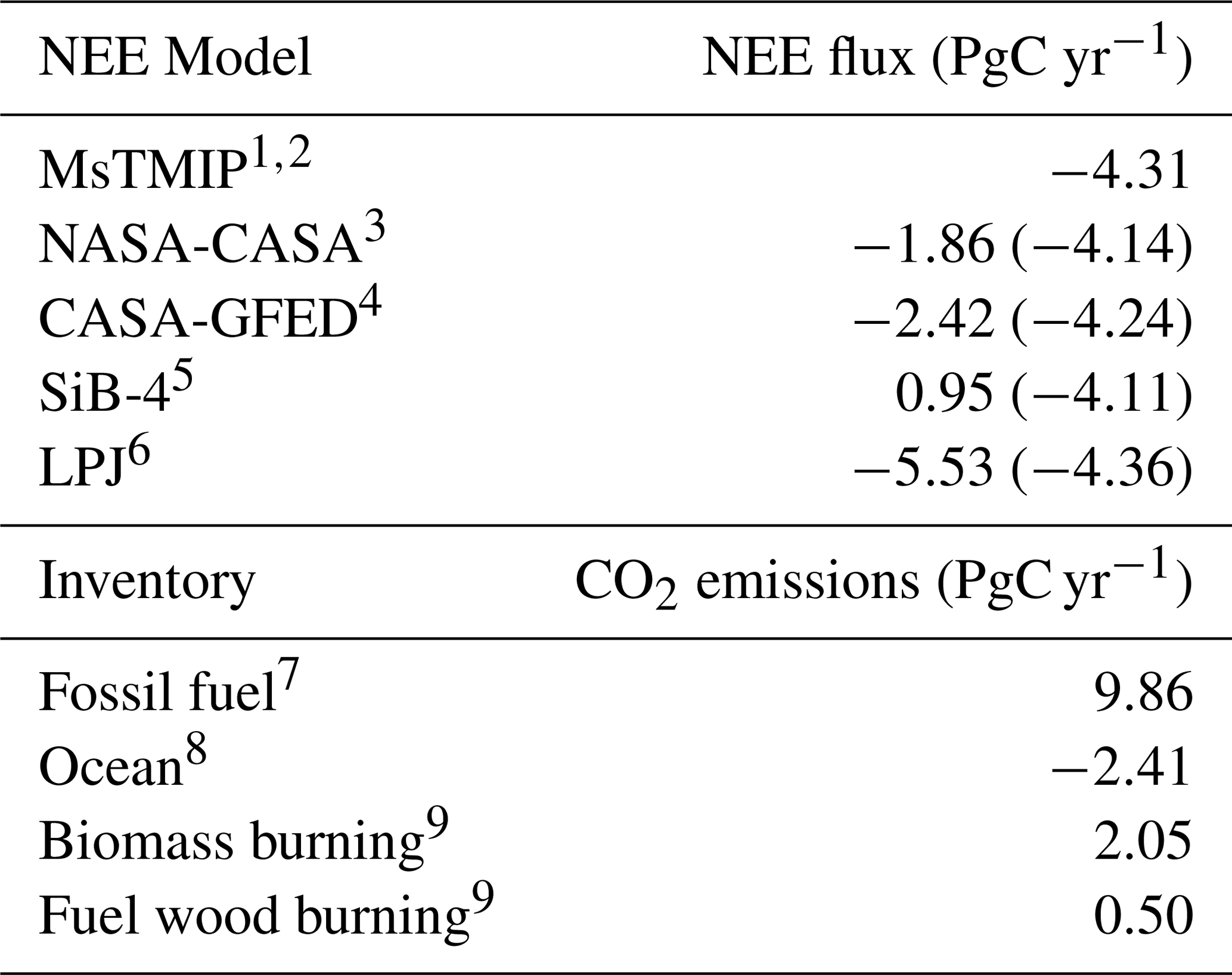
¹ The MsTMIP NEE dataset is representative of the year 2010 and is an ensemble mean of 15 different NEE models. ² Huntzinger et al. (2013, 2016); Fisher et al. (2016a, b). ³ Potter et al. (1993, 2012a, b). ⁴ Potter et al. (1993); Randerson et al. (1996). ⁵ Haynes et al. (2013); Baker et al. (2013). ⁶ Sitch et al. (2003); Poulter et al. (2014). ⁷ Oda et al. (2018); Nassar et al. (2013). ⁸ CarbonTracker CT2016; Peters et al. (2007). ⁹ CASA-GFED3; van der Werf et al. (2004, 2006, 2010).

2.2 GEOS-Chem model

The GEOS-Chem chemical transport model (CTM) (Bey et al., 2001) used in this study has the capability to run forward CO₂ simulations (Suntharalingam et al., 2004; Nassar et al., 2010) and corresponding adjoint model calculations (Henze et al., 2007; Liu et al., 2014). In this study, we use the GEOS-Chem adjoint version 35 (http://wiki.seas.harvard.edu/geos-chem/index.php/GEOS-Chem_Adjoint; last access: 27 January 2017), which is compatible with version 8-02 of the GEOS-Chem forward model. Liu et al. (2014) tested the accuracy of the GEOS-Chem CO₂ adjoint system, which has been used for several CO₂ inverse modeling studies (e.g., Liu et al., 2017; Bowman et al., 2017; Deng et al., 2014). The model is driven with assimilated meteorological fields from the GEOS-FP model of the NASA Global Modeling Assimilation Office (GMAO). The GEOS-FP meteorology fields have a native horizontal resolution of $\mathrm{0.25}{}^{\circ }\times \mathrm{0.3125}{}^{\circ }$ and 72 native hybrid sigma-pressure vertical levels from the Earth's surface to 0.01 hPa. We conduct simulations with a coarser spatial resolution ($\mathrm{4.0}{}^{\circ }\times \mathrm{5.0}{}^{\circ }$) with 47 reduced vertical levels to attain reasonable computational efficiency.

2.3 Non-NEE CO₂ fluxes

To simulate concentrations of atmospheric CO₂, we used several land and ocean CO₂ flux inventories in addition to the NEE estimates from the prior biosphere models (global annual budgets listed in Table 1). This study used the year-specific fossil fuel and cement production inventory from the Open-source Data Inventory for Anthropogenic CO₂ (ODIAC-2016) developed by Oda et al. (2018). Following the approach of Nassar et al. (2013), the monthly ODIAC-2016 inventory is converted from the native temporal variability into diurnal (hourly) and weekday/weekend variability (courtesy of Sourish Basu and the OCO-2 Science Team). Wild fire emissions and fuel wood burning emissions were taken from the 3-hourly Global Fire Emissions Database (GFED3). Shipping emissions are from the International Comprehensive Ocean-Atmosphere Data Set (ICOADS; Corbett and Koehler, 2003; 2004), and aviation emissions are from the Aviation Emissions Inventory Code (AEIC; Olsen et al., 2013). We used 3-D chemical production of CO₂ from the oxidation of carbon monoxide, methane, and non-methane volatile organic compounds (Nassar et al., 2010). The shipping, aviation and 3-D chemical source are climatological and are taken from the Bowman (2017) dataset. To simulate oceanic CO₂ fluxes, we apply the year-specific 3-hourly posterior estimates from the CarbonTracker 2016 (CT2016) model constrained with in situ data (Peters et al., 2007; http://carbontracker.noaa.gov, last access: 22 August 2017). All emission inventories, except the NEE fluxes, are kept constant between the different inverse model simulations.

Table 2 Summary of the different OSSEs conducted during this work.

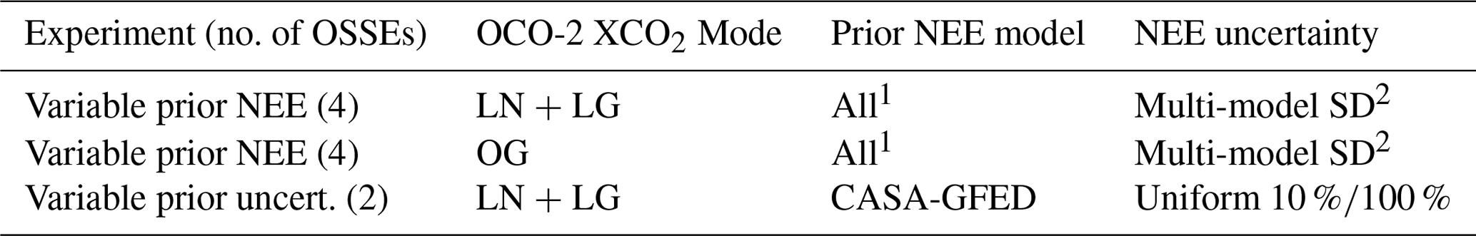
¹ NASA-CASA, CASA-GFED, SiB-4 and LPJ. ² SD denotes standard deviation.

2.4 Observing system simulation experiments (OSSEs)

2.4.1 OSSE framework

This study conducted several OSSEs to assess the impact of prior biospheric CO₂ models and associated prior uncertainty specifications on posterior estimates of NEE when assimilating OCO-2 data. To assess the impact of prior fluxes, we conduct four baseline OSSEs (using the four prior biosphere models) assimilating synthetic land nadir (LN) and land glint (LG) observations together, plus an additional four OSSEs using just ocean glint (OG) observations. These OSSE simulations were designed in such a way that the differences in posterior NEE estimates are due solely to the choice of prior biospheric flux (e.g., identical initial atmospheric CO₂ conditions, non-NEE fluxes, OCO-2 sampling frequency, observational data uncertainty, and so on). Furthermore, to assess the impact of prior uncertainty specifications, we conduct two additional OSSEs (in addition to our baseline prior uncertainty assumption described in Sect. 2.4.5) with synthetic LN and LG observations using prior error set uniformly to 10 % and 100 % of a particular prior NEE flux (CASA-GFED). Table 2 shows the summary of OSSEs conducted for this study. During all OSSE simulations NEE and oceanic CO₂ fluxes are optimized, with all other sources kept constant, in order to be consistent with the methods commonly used by inverse modeling systems focused on estimating NEE. We optimize oceanic fluxes along with NEE, although the same ocean fluxes were used for the truth and the prior in all OSSE simulations (Sect. 2.3) for simplicity and because the terrestrial NEE fluxes are the focus of this work. It is noteworthy that the assimilation of land or ocean data do not in fact produce substantial deviations from the truth over the TransCom-3 oceanic regions (Fig. S2). For all OSSE simulations, an assimilation window of 18 months covering the period from 1 August 2014 to 31 January 2016 was applied. NEE/oceanic fluxes are optimized for every month of the assimilation window at each surface grid box in the GEOS-Chem model. The analysis of prior and posterior NEE fluxes is for all months in 2015, treating the other months as spin-up and spin-down periods.

2.4.2 Initial CO₂ concentrations

We use identical initial atmospheric concentrations of CO₂ on 1 August 2014 for (1) the GEOS-Chem forward model simulations generating synthetic XCO₂ using the true NEE fluxes (Sect. 2.4.3) and (2) for all of the OSSEs using variable prior biosphere model predictions. The initial CO₂ concentrations were generated by running the GEOS-Chem forward model for 2 years using the true MsTMIP NEE and other non-NEE CO₂ sources. The restart file used for this 2-year forward model run was taken from an earlier GEOS-Chem model simulation constrained with in situ observations (personal communication from Ray Nassar) in order to represent a realistic initial condition.

2.4.3 Synthetic OCO-2 retrievals

In this study, we used synthetic satellite data that are directly representative of version 8 of the OCO-2 product. The OCO-2 satellite sensor is in sun-synchronous polar orbit with a repeat cycle of 16 days and a local overpass time in the early afternoon (Crisp et al., 2017). OCO-2 has three different viewing modes: soundings over land from LN and LG and over oceans from OG. The algorithm from O'Dell et al. (2012) is used to retrieve column-average dry air mole fraction of CO₂ (XCO₂) and other retrieval variables. The retrieval of OCO-2 XCO₂ is expressed as Eq. (1) using a prior CO₂ vertical profile (c_a) and prior CO₂ column (XCO_2(a)) value:

$$\begin{array}{}\text{(1)}& {\mathrm{XCO}}_{\mathrm{2}}={\mathrm{XCO}}_{\mathrm{2}\left(a\right)}+{\mathit{a}}^T\left(\mathit{c}-{\mathit{c}}_{\mathrm{a}}\right),\end{array}$$

where c is the true profile of CO₂ concentrations and a is the column averaging kernel. The individual soundings of OCO-2 are at a fine resolution (24 spectra per second with < 3 km² spatial resolution per sounding), leading to a very large data volume (Crisp et al., 2017). This level of detail is lost when the measurements are used in global inverse models with much coarser spatial resolution, with numerous individual OCO-2 soundings occurring in a single model grid box. In addition, each sounding does not really provide an independent piece of information to the inversion system due to spatial and temporal error correlations. Therefore, we use 10 s averages of the individual XCO₂ soundings similar to those developed/described in Basu et al. (2018), although these soundings are from an updated version with the file name “OCO2_b80_10sec_WL04_GOOD_v2.nc”. These 10 s data contain averages of retrievals with a “good” quality flag and a “warn level” from 1 to 4. Note that in this study we do not use actual retrieved 10 s XCO₂ values for our OSSEs; however, synthetic XCO₂ data were generated corresponding to the spatiotemporal sampling frequency of version 8 OCO-2 10 s data. These synthetic 10 s XCO₂ data are calculated with the CO₂ concentration profile simulated using the GEOS-Chem forward model (using MsTMIP as the NEE flux model). In this manner we produced synthetic XCO₂ data that are representative of the true atmosphere corresponding to the true NEE fluxes used in this study. We archived these synthetic XCO₂ data and applied them for all OSSEs conducted.

2.4.4 Inverse modeling approach

The transport of atmospheric CO₂ is simulated using GEOS-Chem along with prescribed surface fluxes as input data (see Table 1). Subsequently, the GEOS-Chem 4D-Var inverse modeling system assimilates synthetic OCO-2 XCO₂ data to estimate the posterior/optimized monthly mean NEE and oceanic fluxes at each surface grid box of the model. The GEOS-Chem adjoint system applies the L-BFGS numerical optimization algorithm with a no-bound option (Liu and Nocedal, 1989). Posterior monthly averaged NEE/oceanic fluxes (x) are inferred for each surface model grid box by optimizing a vector of scaling factors σ_j for the jth model grid box as follows:

$$\begin{array}{}\text{(2)}& x_j={\mathit{\sigma }}_j{x}_{a,j},\end{array}$$

where x_a represents the monthly mean prior NEE/oceanic fluxes. Scaling factors are assumed to be unity at the first iteration (that is, the prior NEE flux itself is used). The inversion system, as described below, optimizes the scaling factor applied to the monthly mean fluxes and the posterior scaling factors are then used to scale prior fluxes to infer posterior CO₂ fluxes.

For each iteration, the inversion system uses the forward model simulated profiles of CO₂ concentrations mapped to OCO-2 retrieval levels (f(x)) in each model grid box in order to compare them with the synthetic OCO-2 observations (y). The observation operator (M) represents the model simulated XCO₂ corresponding to each synthetic OCO-2 retrieval,

$$\begin{array}{}\text{(3)}& M={\mathrm{XCO}}_{\mathrm{2}\left(a\right)}+{\mathit{a}}^T\left(\mathit{f}\left(\mathit{x}\right)-{\mathit{c}}_{\mathrm{a}}\right)\end{array}$$

using XCO_2 (a) and c_a from the retrieval (see Eq. 1). The optimization approach used in this work defines the 4D-Var cost function (J) as follows:

$$\begin{array}{}\text{(4)}& \begin{array}{rl}J\left(\mathit{\sigma }\right)& ={\displaystyle \frac{\mathrm{1}}{\mathrm{2}}}{\sum }_i(M_i-{\mathit{y}}_i{)}^T{\mathbf{R}}_i^{-\mathrm{1}}\left(M_i-{\mathit{y}}_i\right)\\ & +{\displaystyle \frac{\mathrm{1}}{\mathrm{2}}}(\mathit{\sigma }-{\mathit{\sigma }}_{\mathrm{a}}{)}^T{\mathbf{P}}^{-\mathrm{1}}\left(\mathit{\sigma }-{\mathit{\sigma }}_{\mathrm{a}}\right),\end{array}\end{array}$$

where y_i is the vector of synthetic OCO-2 XCO₂ data across the assimilation window, with “i” being the number of XCO₂ data. Furthermore, R and P are the observational error covariance matrix and prior error covariance matrix, respectively.

2.4.5 Prior flux uncertainty

For a perfect optimization, the prior error covariance matrix (P) assumed in the inversion should equal the uncertainty of the prior model used. However, the estimation of prior error statistics is a challenging task due to the lack of flux evaluation data. Previous studies have used a range of techniques to characterize prior error covariance such as developing the full error covariance matrix with assumed error correlations (Basu et al., 2013), using a fraction of heterotrophic respiration (Basu et al., 2018), conducting Monte Carlo simulations (Liu et al., 2014), using standard deviations and absolute differences between several different prior flux models (Baker et al., 2006a, 2010), using continuous in situ measurements of CO₂ flux compared to model simulations to inform prior errors (Chevallier et al., 2006), and applying globally uniform prior flux uncertainty values to satisfy the posterior χ²(normalized cost function) =1 criteria (Deng et al., 2014). During this study, a 1σ standard deviation (SD) of the four prior biosphere models (see Sect. 3.1 for the description of SD values) is considered to be the measure of uncertainty in the prior knowledge of bottom-up model predicted biospheric CO₂ fluxes. The SD of the four prior NEE estimates is applied in the prior error covariance matrix and no spatial or temporal correlations are taken into account. This assumption is reasonable, as optimized fluxes are at coarse spatiotemporal scales (monthly mean fluxes at horizontal resolutions of > 400 km²), and is representative of the majority of inverse modeling studies assimilating CO₂ satellite data (e.g., Baker et al., 2010; Liu et al., 2014; Deng et al., 2014). Finally, as the inverse modeling system applied in this work optimizes scaling factors, we use the square of the fractional prior error in the P matrix, where the fractional error is calculated for each individual prior model as the SD of the four prior models divided by the absolute value of the NEE magnitude. For generating prior error for the oceanic fluxes, we follow the same method we adopted for generating prior errors in NEE. The SD of four different state of the art oceanic CO₂ flux datasets – NASA-CMS CO₂ oceanic flux (from Bowman, 2017), CarbonTracker 2016 prior ocean data (CT2016; http://carbontracker.noaa.gov, last access: 22 August 2017), Takahashi et al. (2009), and Landschützer et al. (2016, 2017) – was calculated to generate prior error values.

2.4.6 XCO₂ uncertainty

As described in Sect. 2.4.3, the synthetic XCO₂ used in this study is calculated at the spatiotemporal sampling frequency of the OCO-2 10 s average dataset. Although we use synthetic XCO₂, we apply the same observation error statistics generated with the actual OCO-2 XCO₂ 10 s dataset in order to develop the observational error covariance matrix (R). The final observation error for the 10 s average data is generated as a quadratic sum of the retrieval error from individual OCO-2 soundings, 10 s averaging error, and a “model representation error” as described in Basu et al. (2018). Similar to the treatment of prior error statistics, we neglect observation error correlations and assume a diagonal observational error covariance. No random perturbations were added to the synthetic XCO₂ used in this study, as the goal of this work was not to quantify the analytical posterior flux uncertainty but instead to analyze the spread among posterior NEE estimates. We note that other inverse modeling groups assimilating OCO-2 data also do not add random perturbations to the data and use the same error statistics generated along with the OCO-2 10 s product that are applied in this study (e.g., Basu et al., 2018; Crowell et al., 2019). During this study the square of the observation error for the 10 s average data was applied as the diagonal in the R matrix. From our initial OSSE tests it was determined that the use of 10 s error statistics led to posterior χ² (normalized cost function) values that were much lower than unity. Therefore, we divided the 10 s error values uniformly by a factor of 5 to approximately satisfy the χ²=1 criteria for all of the OSSEs. This deflation procedure reduced the average 10 s observational error values for LN+LG (OG) data from ∼1.5 (∼0.9) to ∼0.3 (∼0.2) ppm. These procedures give more confidence to the observational data and lead to results in this study which can be assumed as the lower limit of the impact of prior model flux and uncertainty statistics in inverse model estimates.

2.4.7 Evaluation of OSSE results

During this study, the posterior NEE values from the OSSEs are compared to the true fluxes to assess accuracy and are also intercompared to assess the spread in posterior estimates due to the assumed prior NEE and prior error statistics. The primary statistical parameters used to evaluate the spread in posterior NEE fluxes are the SD (hereafter the term “spread” will be used to represent SD) and range (difference between maximum and minimum in NEE). The SD/spread and range of posterior NEE estimates, when using the different prior models, will provide an understanding of the spatiotemporal residual impact of the prior models in top-down estimates of global/regional NEE fluxes when assimilating OCO-2 data.

In order to evaluate the spatiotemporal variability of prior and posterior regional NEE fluxes, we aggregate individual model grid boxes to the TransCom-3 land regions (TransCom-3 regions illustrated in Fig. 1). To further interpret the OSSE results, we produce additional classifications of three broad hemisphere-scale TransCom-3 land regions: northern land (NL), tropical land (TL), and southern land (SL). TL includes tropical South America, North Africa, and tropical Asia; SL includes South American temperate, South Africa, and Australia; and NL includes the other five land regions. The evaluation of the SD and range of prior model and posterior/optimized NEE fluxes were calculated for the 11 individual TransCom-3 regions, for the 3 hemisphere-scale TransCom-3 regions, and globally. Throughout the paper, seasonally averaged prior and posterior NEE fluxes will be discussed and these seasons are presented with respect to the Northern Hemisphere.

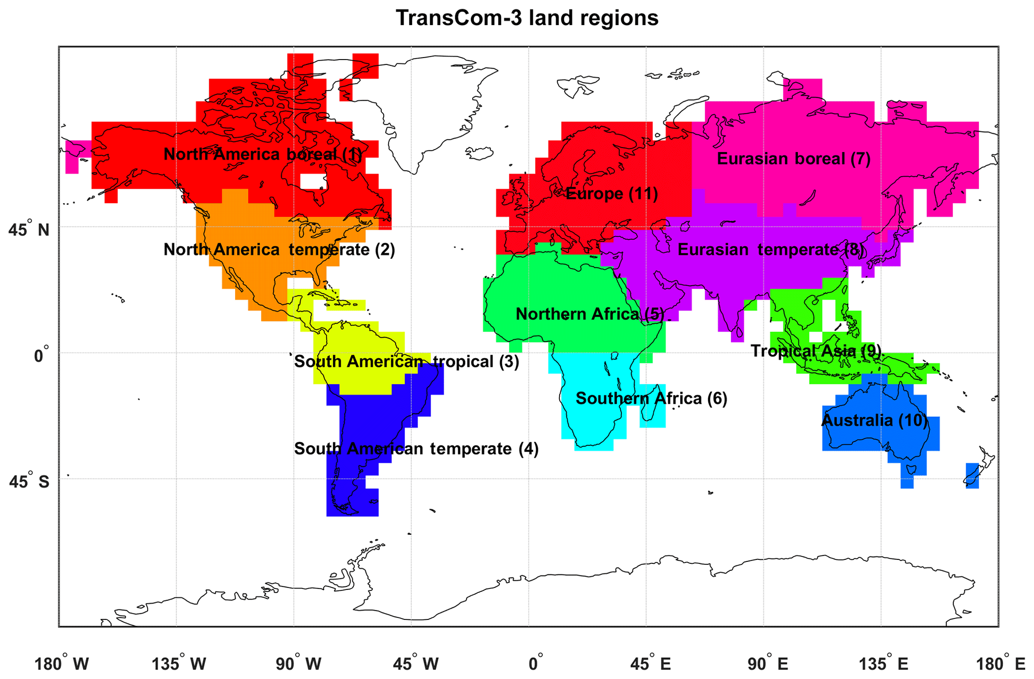
Figure 1 The TransCom-3 land region boundaries used to aggregate CO₂ fluxes for evaluation.

2.4.8 Pseudo data assimilations

In order to test our OSSE framework, we first run four “pseudo” (hereafter quotation marks will be omitted) experiments by conducting inverse modeling studies using pseudo surface observations. These test OSSE simulations were conducted for 5-month assimilation windows for two separate seasons, November 2014 to March 2015 (analysis for winter, DJF) and May to September 2015 (analysis for summer, JJA), using all four prior model NEE values separately. Simulated hourly concentrations of CO₂ for all surface grid boxes of GEOS-Chem are taken as pseudo surface observations. In order to check whether the model framework can converge to the truth, a simple controlled experiment was performed assuming a very small observational data uncertainty (0.001 %) and with the prior flux uncertainty set equal to the absolute magnitude of the truth – prior NEE (divided by the absolute value of the NEE magnitude for that respective prior model). The robustness of the flux inversions conducted in the subsequent sections is validated by the results of these pseudo tests. Figure S3 shows the results of the four pseudo tests using the four different NEE flux model predictions as the prior information. From this figure it is apparent that, regardless of the prior NEE assumed, posterior NEEs were able to reproduce the truth with near perfect accuracy for all TransCom-3 regions, with the range between the posterior NEEs typically approaching ∼0 PgC yr⁻¹. This test also demonstrates that a “perfect” assimilation (using uniform and dense surface data coverage, highly accurate data, and known/loose prior uncertainty) is almost insensitive to the prior assumed. Having tested the robustness of our inversion setup, we feel confident in presenting the output from our OSSE framework, using synthetic OCO-2 remote-sensing data, in the following sections.

3 Results and discussion

3.1 Prior NEE fluxes

Figure 2 shows the seasonally averaged multi-model-mean and SD of the NEE fluxes from the four prior biosphere models used in the OSSE simulations (individual prior model and true seasonally averaged NEE fluxes are displayed in Fig. S4). This figure shows the main features of NEE that are expected, such as the Northern Hemispheric fall/winter maximum in R_e and summer maximum in GPP due to the seasonality of photosynthesis and respiration. Figure 2 also shows the spread of the four prior model fluxes (used as prior uncertainty), which is typically highest over the temperate regions of the Northern Hemisphere in the spring and summer and high in the tropical regions during all seasons (the left panels of Fig. 3 shows a spatial map of the corresponding range of the four prior model fluxes). Furthermore, Fig. S5 shows the time series of monthly mean prior NEE fluxes, and the corresponding prior error uncertainty (error bars), for the individual prior models. From this figure it can be seen that the 1σ prior uncertainties for the global land are ∼50 %–70 % of the total NEE for the different prior models, with variability among other TransCom-3 land regions.

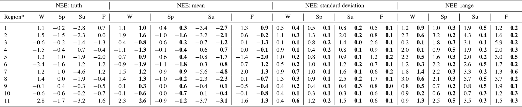
Table 3 Data corresponding to Fig. 6. Seasonally averaged NEE (PgC yr⁻¹) averaged over the 11 TransCom-3 land regions (refer to Fig. 1) for the MsTMIP (truth), multi-model prior mean, and multi-model posterior mean (PgC yr⁻¹). The differences between the prior and posterior model NEE values are presented as SD (1σ) and range. Prior model values are presented in standard font and posterior estimates are in bold. Seasons are represented as Winter (W), December–February; Spring (Sp), March–May; Summer (Su), June–August; and Fall (F), September–November. The synthetic observations in these OSSE simulations correspond to the OCO-2 LN+ LG observing modes.

^* TransCom-3 region name and location displayed in Fig. 1.

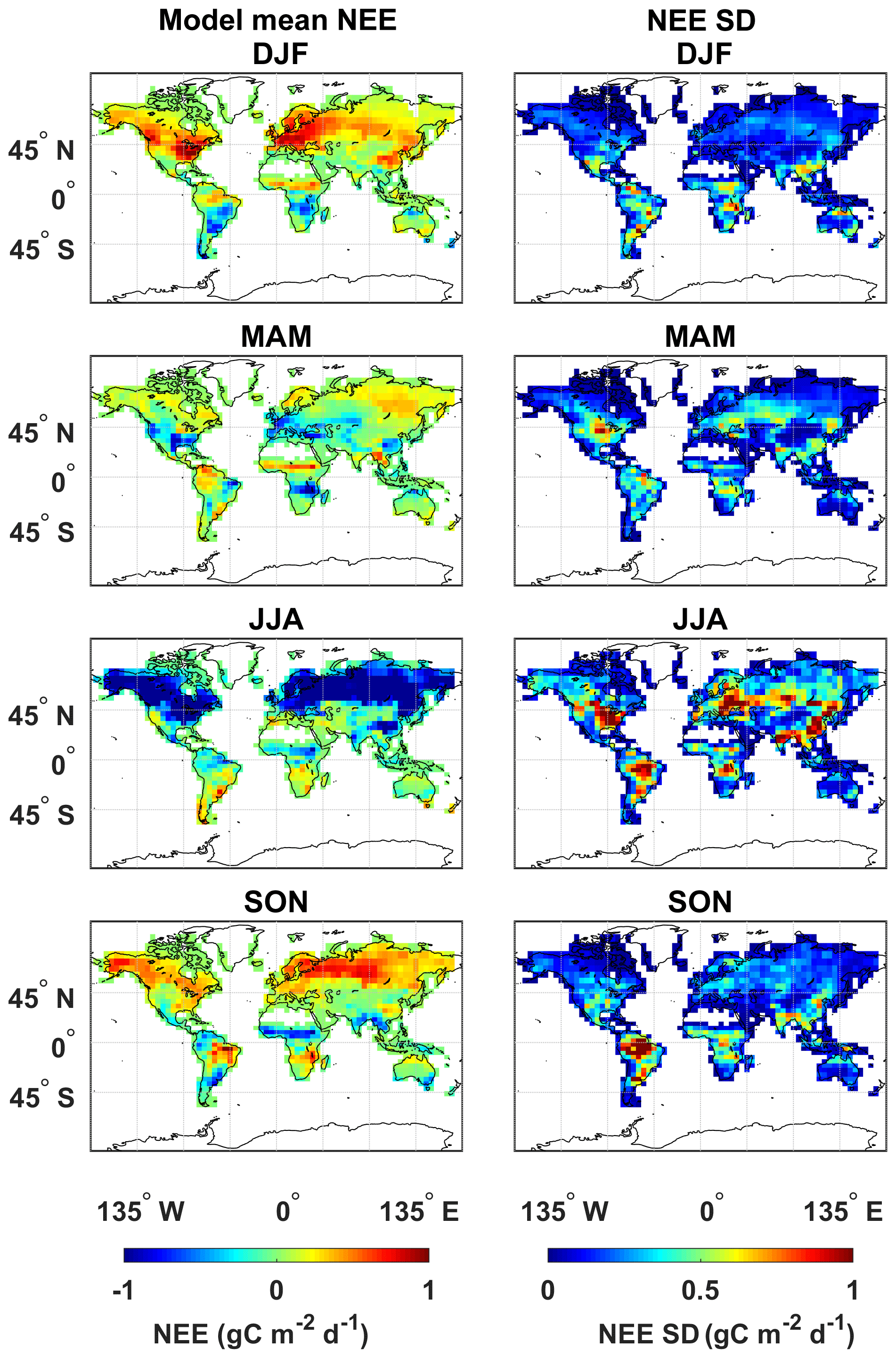
Figure 2 Prior multi-model (NASA-CASA, CASA-GFED, SiB-4, and LPJ biosphere models) seasonally averaged NEE (gC m⁻² d⁻¹; left column) and NEE SD (standard deviation) (gC m⁻² d⁻¹; right column) for the year 2015.

Table 3 displays the statistics of the prior NEE multi-model-mean and SD and range for the 11 individual TransCom-3 land regions. The SD values for prior NEE fluxes range from ∼20 % to frequently > 100 % of the multi-model NEE mean for different regions/seasons with significant NEE fluxes (hereafter this refers to regions/seasons with NEE flux ≥0.5 PgC yr⁻¹). When comparing the magnitude of NEE between the four prior models, it can be seen (from Table 3) that the range of the NEE values is large in some regions (up to 6 PgC yr⁻¹). In general, all regions/seasons tend to have at least an ∼1 PgC yr⁻¹ range among the four prior models, indicating the large diversity in NEE predicted by current bottom-up biosphere models (Table 3). Figure S5 shows the time series of monthly mean NEE for individual prior models averaged over the globe, hemispheric-scale land regions (NL, TL, and SL), and the 11 individual TransCom-3 land regions. It can be seen from this figure that the majority of the seasonality in the global NEE flux is controlled by the NL regions. Figure S5 also shows that the spread in prior NEE fluxes is larger in general for TL and SL regions compared with the NL, except for the North American temperate region. Furthermore, when focusing on individual models, differences in NEE seasonality are evident. The impact of these differences among the four prior biospheric CO₂ flux models on simulated XCO₂ and posterior estimates of global/regional NEE fluxes is evaluated in the following sections.

3.2 Simulated XCO₂

Figure 4 shows the number of observations sampled in the OCO-2 LN and LG modes during the different seasons of 2015 summed in each model grid box. Large spatiotemporal variability can be seen in the OCO-2 observation density, with the largest values over regions with minimal cloud coverage (e.g., desert regions of North/South Africa, Middle East, Australia, and so on.). The opposite is true for many tropical regions (e.g., Amazon, central Africa, tropical Asia, and so on.) where cloud occurrence is prominent and the number of OCO-2 observations is lowest. From Fig. 4 it can also be seen that the OCO-2 observation density has noticeable seasonality. For example, during the winter months low numbers of OCO-2 observations are made in the northern boreal regions and the largest amounts are observed during the summer. Furthermore, larger numbers of OCO-2 observations are made in the SL during the summer (JJA) compared with other seasons.

Figure 3 Seasonally averaged NEE range (gC m⁻² d⁻¹) of the four prior biosphere models (NASA-CASA, CASA-GFED, SiB-4, and LPJ) (left column) and posterior estimates (right column) from the OSSE simulations. The synthetic observations in these OSSE simulations correspond to the OCO-2 LN+LG observing modes.

Figure 4 Total number of OCO-2 LN and LG XCO₂ observations (left column) and the corresponding seasonally averaged multi-model (NASA-CASA, CASA-GFED, SiB-4, and LPJ biosphere models) mean GEOS-Chem-simulated prior XCO₂ (right column) in 2015.

The seasonally averaged multi-model-mean GEOS-Chem simulated XCO₂ using the four prior model NEE fluxes is shown in the right column of Fig. 4. The most notable feature in this figure is the Northern Hemisphere seasonality, with higher XCO₂ concentrations in the winter months and lowest XCO₂ values in the growing seasons of the summer. Seasonality in model-predicted XCO₂ values is also evident in the TL and SL, with largest values in the autumn and lowest values in the spring. Figure 5 (left column) shows the range of XCO₂ values simulated using the four prior model NEE fluxes. The differences between individual model simulations of XCO₂ values deviated among themselves by up to ∼10 ppm. These large differences in XCO₂ values across the four different prior NEE flux models show that the choice of prior NEE has a large impact on simulated XCO₂ values.

3.3 Optimized global NEE fluxes

From Table 1 it can be seen that annual global mean posterior NEE flux, when using the different prior models and assimilating synthetic LN+LG OCO-2 XCO₂, ranges from −4.11 to −4.36 PgC yr⁻¹, which is generally close in magnitude to the true flux of −4.31 PgC yr⁻¹. Although these posterior NEEs generally converged to the truth, there are some remaining differences, with an annual global mean posterior NEE range of 0.25 PgC yr⁻¹ (∼6 % of the multi-model-mean posterior NEE; Table 1). From the results of the OSSE simulations, it was found that the spread and range in XCO₂ simulated using the optimized posterior NEE fluxes was greatly reduced compared with the spread in XCO₂ simulated using prior NEE fluxes. This is evident from the right column of Fig. 5 where XCO₂ values simulated using posterior NEE fluxes differ among themselves by < 0.5 ppm, which is greater than an order of magnitude lower, on average, than the spread among XCO₂ values simulated using prior NEEs.

Figure 3 shows the spatial distribution of the range of prior and posterior NEEs. As expected, the range in optimized posterior NEE flux estimates starting from the four separate prior models was substantially reduced compared with the spread in prior NEE fluxes. However, the posterior NEE fluxes for individual surface grid boxes of the model still depict some residual range among the posteriors, with the largest residuals being found across South America and South Africa in all seasons and in temperate regions of the Northern Hemisphere in the spring months. As shown in Fig. 3, the geographical pattern of the range of prior and posterior NEEs does not indicate any noticeable correlations. From comparing Figs. 3 and 5, it is apparent that the spread in posterior XCO₂ is significantly reduced in all regions of the globe compared with prior model simulations; however, while posterior NEE values are reduced compared to the prior, noticeable residual spread remains in some regions. This emphasizes the fact that the OSSEs successfully converge to match the synthetic OCO-2 XCO₂ values by optimizing NEE in different ways depending on the prior NEE model used. The following sections investigate the regional differences in posterior NEE estimates due to the residual impact of prior biospheric CO₂ flux predictions.

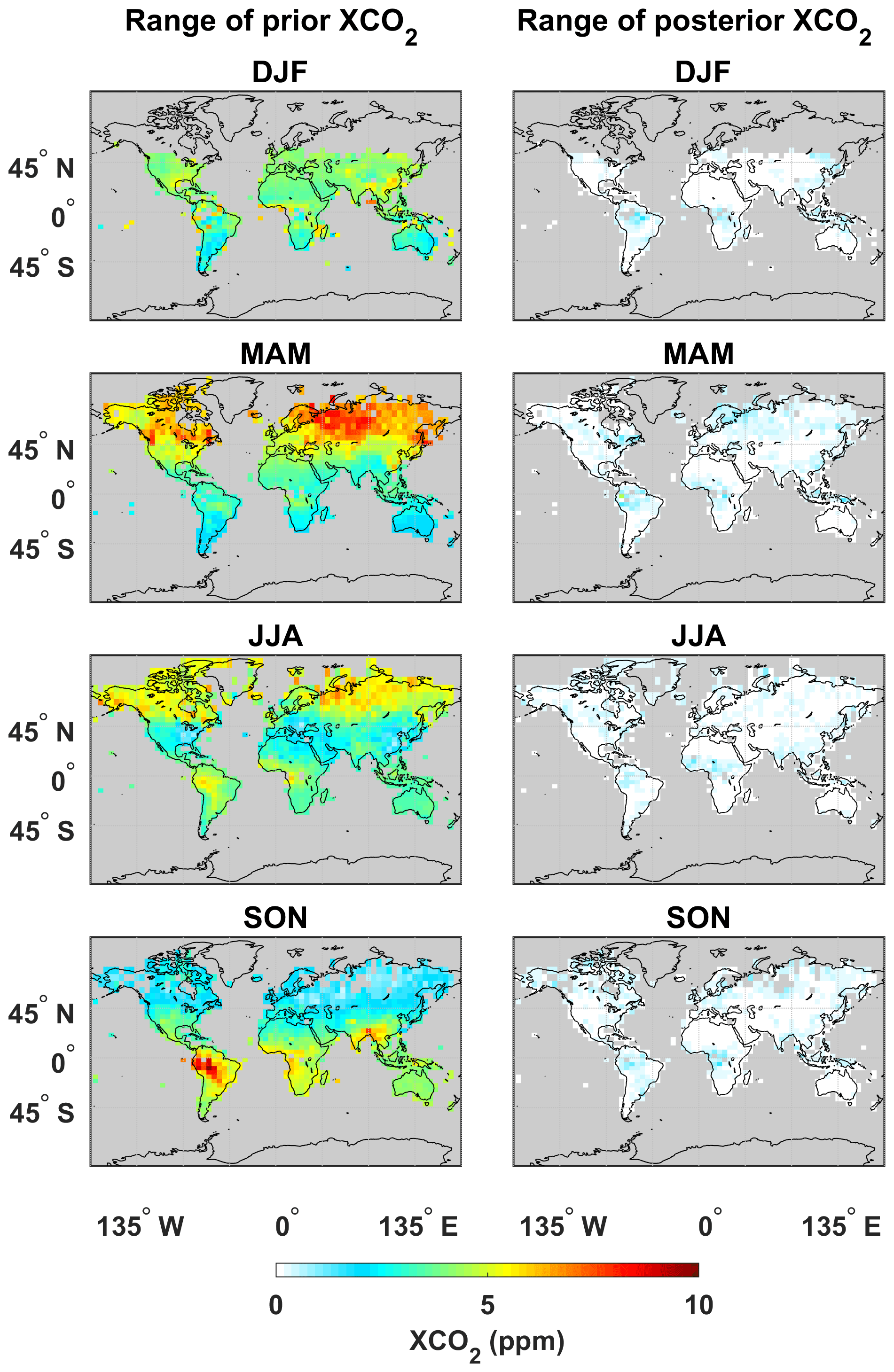
Figure 5 Seasonally averaged XCO₂ range from GEOS-Chem forward model simulations using the four prior biosphere models (NASA-CASA, CASA-GFED, SiB-4, and LPJ) (left column) and the corresponding posterior estimates (right column) from the OSSE simulations. The synthetic observations in these OSSE simulations correspond to the OCO-2 LN+LG observing modes.

3.4 Optimized regional NEE fluxes

Figure 6 shows the seasonally averaged true, prior, and posterior NEE flux values for the 11 individual TransCom-3 land regions (with detailed statistics in Table 3 and monthly mean time series in Fig. S6). The first thing noticed from this figure is that all posterior NEE values, using variable priors, tend to reproduce the truth in most TransCom-3 land regions. From Fig. 6 it can also be seen that the assimilation of synthetic OCO-2 LN+LG XCO₂ retrievals resulted in a large reduction in the range among the four modeled NEE values (Table 3 shows the corresponding SD values). The reduction in the SD of NEE (also known as uncertainty reduction) in most regions/seasons, calculated as 100× (1− (posterior NEE SD)/(prior NEE SD)), is generally > 70 % and up to 98 %. However, the range of seasonal mean posterior NEEs over individual TransCom-3 regions is still as large as 1.4 PgC yr⁻¹ when applying different prior NEEs, with the largest ranges occurring in northern boreal regions (North America boreal, Eurasian boreal, and Europe) in the winter months. During the spring and summer months, regions in the TL (e.g., tropical Asia) and SL (e.g., South American temperate and South Africa) have ranges in posterior NEEs up to ∼0.5 PgC yr⁻¹. The larger residual range among posterior NEE estimates for winter months in northern boreal regions is likely due to the insufficient OCO-2 observations during this time (see Fig. 4), while the larger range in the TL and SL regions is due to differences in the priors (see Fig. 2). This demonstrates that the impact from the prior model has regional and seasonal variability depending on (1) the spatiotemporal flux variabilities inherent in prior NEEs and (2) the observation density and coverage of synthetic OCO-2 data. Figure 6 and Table 3 show that the seasonally averaged posterior NEE spread varies from ∼10 % to ∼50 % of the multi-model-mean for different TransCom-3 land regions with significant NEE fluxes. When evaluating this residual spread in posterior NEEs on a global average, seasonally averaged values ranged from ∼10 % (JJA) to ∼20 % (DJF) of the posterior NEE mean. These statistics reveal that the impact of prior models lead to a much larger spread/range for regional/seasonal posterior fluxes (up to ∼50 %) compared with annual global averaged values (6 %). This emphasizes that while OCO-2 observations on average constrain global, hemispheric, and regional biospheric fluxes, noticeable residual differences in posterior NEE flux estimates remain due to the choice of prior model values. Overall, the results of this evaluation suggest that when intercomparing inverse model results assimilating similar OCO-2 observational data, differences in posterior NEE in regions with significant NEE fluxes could vary by up to ∼50 % when using different prior flux assumptions.

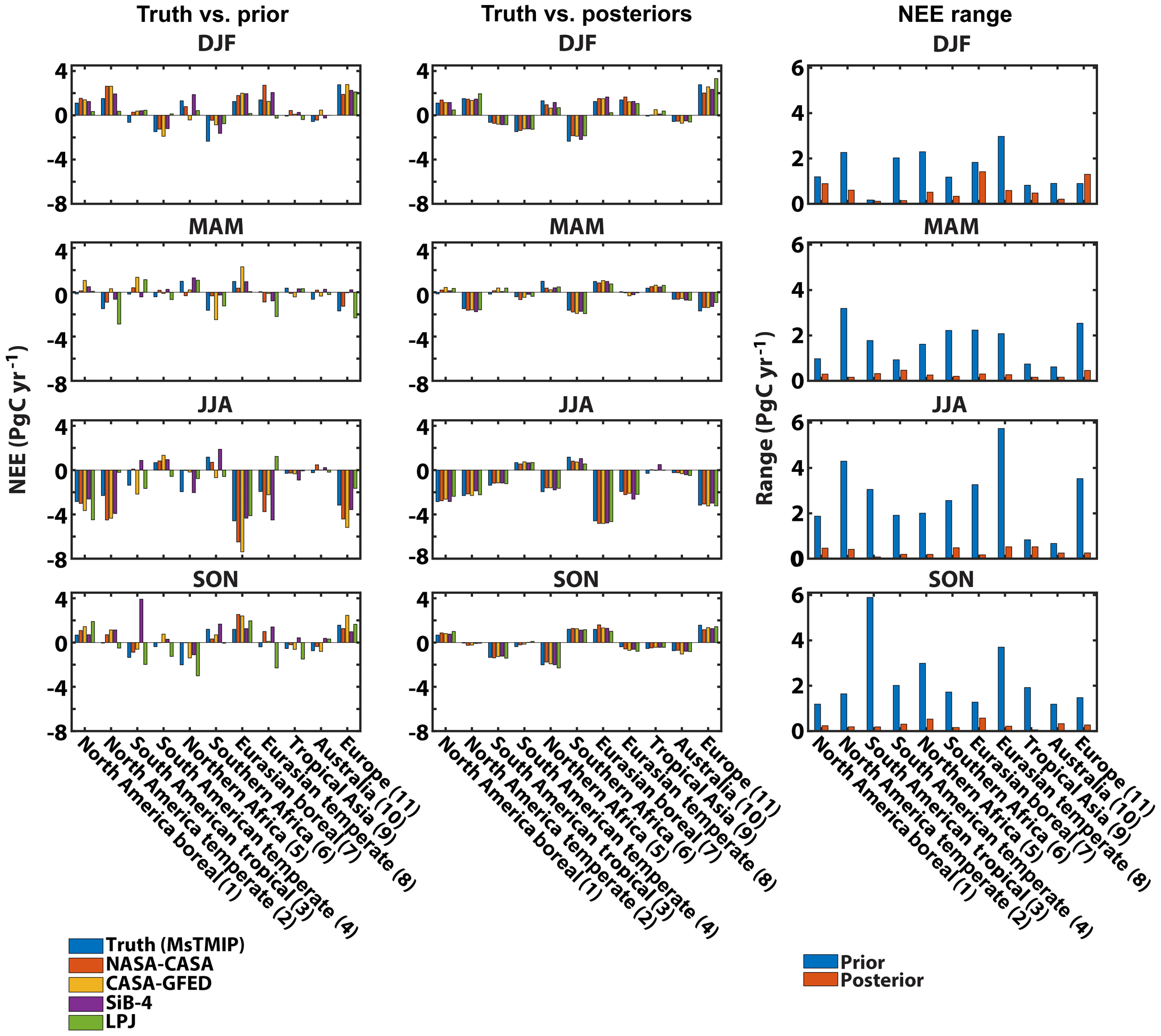
Figure 6 Seasonally averaged NEE averaged over the 11 TransCom-3 land regions from MsTMIP (truth) vs. the prior biosphere models (NASA-CASA, CASA-GFED, SiB-4, and LPJ) (left column), posterior estimates (middle column) from the OSSE simulations, and the corresponding range of prior and posterior NEE estimates (right column). The synthetic observations in these OSSE simulations correspond to the OCO-2 LN+LG observing modes. Detailed statistics of the truth, multi-model means of prior and posterior NEE estimates, standard deviations, and ranges displayed in this figure are listed in Table 3.

3.5 Impact of prior uncertainty

Results of this study have demonstrated the sensitivity of posterior NEE estimates to prior NEE flux assumptions. In this section, the sensitivity of posterior NEE estimates to the assumed prior uncertainty is tested, when assimilating synthetic OCO-2 LN+LG XCO₂ observations. The general importance of prior uncertainty values is highlighted in the TL regions. In these regions the largest differences in prior models are calculated, thus the largest prior uncertainty is assigned, resulting in larger deviations from the prior and posterior NEE spread similar to other TransCom-3 land regions (see Fig. 6). In order to quantify the sensitivity of posterior NEE to prior uncertainty statistics, a single prior NEE flux model (CASA-GFED) is applied in the OSSE framework, with variable prior flux uncertainty assumptions. Two additional OSSE simulations (in addition to the baseline simulations using the SD of the four prior models as the prior uncertainty; see right column of Fig. 2 for SD maps) are performed using prior NEE magnitudes from CASA-GFED and setting the prior uncertainty uniformly as 10 % and 100 % of the CASA-GFED NEE values. Figure 7 shows the results of these additional OSSE simulations over the TransCom-3 land regions. From this figure it can be seen that the range of seasonal mean posterior NEEs over individual TransCom-3 regions vary from ∼0.1 to > 1 PgC yr⁻¹ when applying variable prior error assumptions. Seasonally averaged posterior NEE SD varies from ∼10 % to 50 % of the multi-model-mean for different TransCom-3 land regions with significant NEE fluxes. On a global average, the seasonal-average SD values range from ∼15 % (JJA) to ∼30 % (DJF) of the posterior NEE mean. Note that these posterior NEE SD/range values are similar here to the baseline OSSEs conducted by changing prior NEE flux magnitudes (see Fig. 6). However, when comparing Figs. 7 and 6 (and Fig. S7), it is noticed that posterior NEE estimates are more sensitive to prior error assumptions compared with prior flux values in some seasons/regions of TL and SL (e.g., northern Africa, southern Africa, and South America temperate). It appears that NEE estimates during this study are more sensitive to prior error assumptions when sufficient observations are available and large differences between the prior and truth are present. Also, from Fig. 7 it can be seen that prior uncertainty assumptions in the baseline runs (using SD of prior models) and the assumption of 100 % prior uncertainty tend to reproduce the truth more accurately than NEE estimates using 10 % prior error. Overall, the results demonstrate that the posterior NEE fluxes over TransCom-3 land regions are in general similarly sensitive (up to ∼50 %) to the specification of prior flux uncertainties and the choice of bottom-up prior biospheric NEE model estimates.

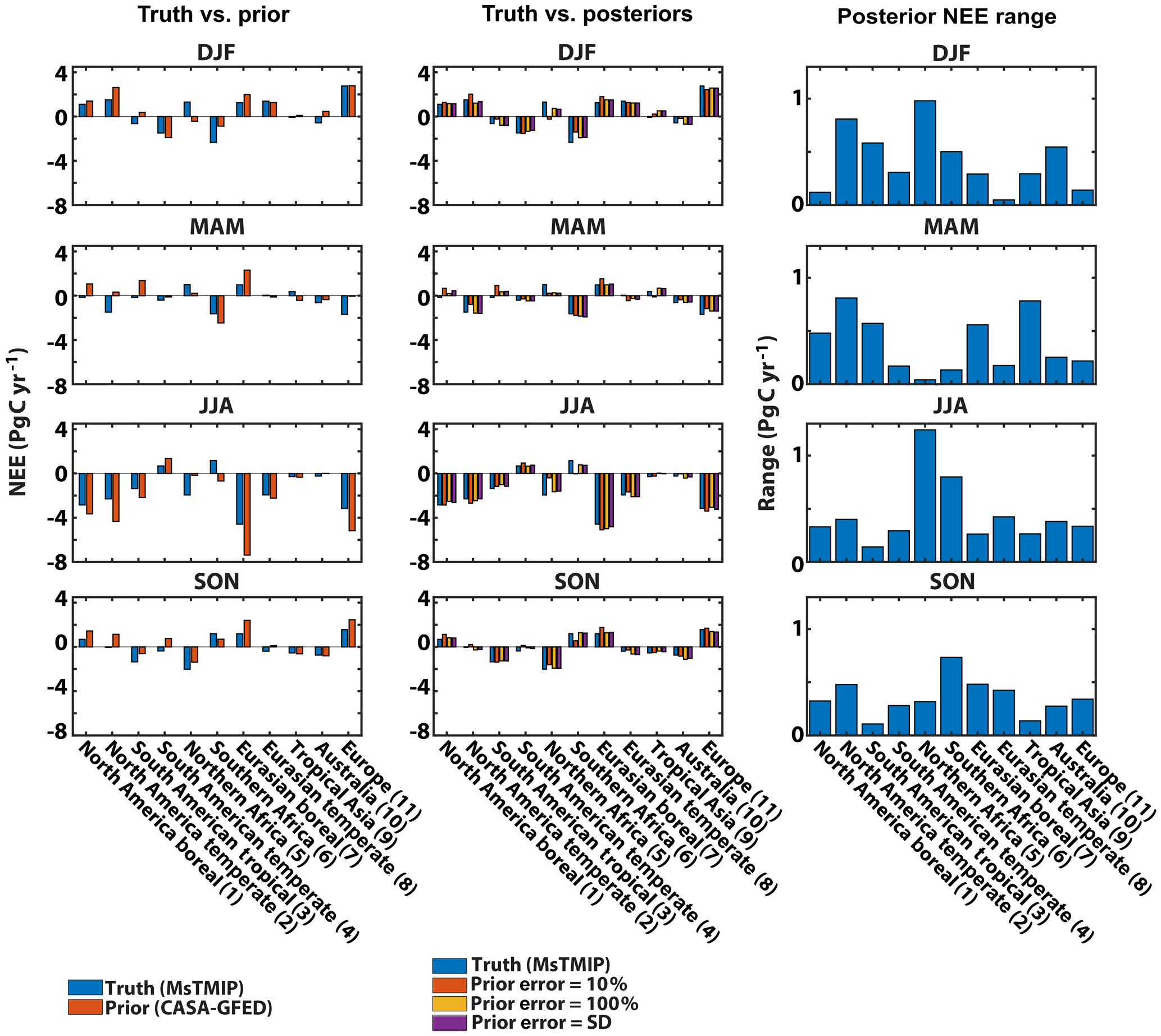
Figure 7 Seasonally averaged NEE averaged over the 11 TransCom-3 land regions from MsTMIP (truth) vs. CASA-GFED prior biosphere model (left column), posterior estimates with the three different prior uncertainties (middle column), and the corresponding range of posterior NEE (right column). The synthetic observations in OSSE simulations correspond to the OCO-2 LN+LG observing modes. Detailed statistics of the truth, prior, multi-model mean of posterior NEE estimates, standard deviations (SD), and ranges displayed in this figure are listed in Table S1 in the Supplement.

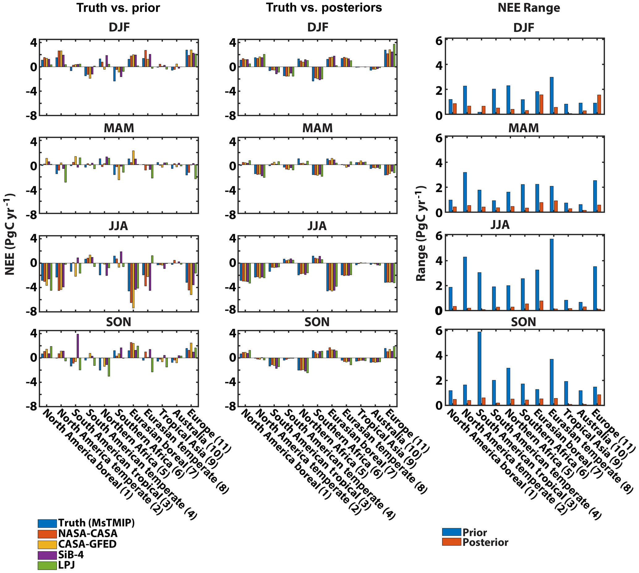
Figure 8 Seasonally averaged NEE averaged over the 11 TransCom-3 land regions from MsTMIP (truth) vs. the prior biosphere models (NASA-CASA, CASA-GFED, SiB-4, and LPJ) (left column), posterior estimates (middle column) from the OSSE simulations, and the corresponding range of prior and posterior NEE (right column). The synthetic observations in these OSSE simulations correspond to the OCO-2 OG observing mode. Detailed statistics of the truth, multi-model means of prior and posterior NEE estimates, standard deviations, and ranges displayed in this figure are listed in Table S2.

3.6 OCO-2 ocean data

This portion of the study investigates the impact of assimilating OCO-2 OG XCO₂ data on posterior NEE flux estimates in our OSSE framework. To do this, four additional OSSE simulations were conducted with the four prior model NEEs when only assimilating synthetic OG retrievals (instead of LN+LG) in the inversions (everything else remains the same as in the baseline simulations). Figure 8 shows the results of these four additional OSSE simulations averaged over the TransCom-3 land regions. From these simulations it can be seen that OCO-2 OG indeed reduces the range in posterior NEE flux estimates, when applying different priors, compared with prior model predictions, and can generally reproduce the truth. On average, the spread in posterior NEE fluxes is ∼20 % to ∼50 % of the multi-model-mean for different TransCom-3 land regions with significant NEE fluxes. As expected, the comparison of Figs. 6 and 8 suggests that LN+LG data are better able to constrain biospheric CO₂ fluxes compared with OG data, as the spread among the posteriors is generally lower in assimilations using only LN+LG data (∼70 % lower on a global average) compared with assimilations using only OG data. However, there were some cases where OSSE simulations using OCO-2 OG data alone did in fact result in slightly lower posterior NEE spreads in some TransCom-3 land regions compared with LN+LG assimilation runs (e.g., northern boreal regions during summer months and Australia during winter months). Overall, our OSSE simulations using the OCO-2 OG data demonstrate the importance of these oceanic retrievals to constrain land NEE fluxes, as the posterior NEE range is much lower than prior NEE estimates (see Fig. 8). This generally agrees with previous studies that demonstrated the importance of satellite data over the ocean in constraining NEE fluxes over land regions (e.g., Deng et al., 2016).

4 Conclusions

To the best of our understanding, this is the first study directly quantifying the impact of different prior global land biosphere models on the estimate of terrestrial CO₂ fluxes when assimilating OCO-2 satellite observations. We conducted a series of OSSEs that assimilated synthetic OCO-2 observations applying four state of the art biospheric CO₂ flux models as the prior information. These controlled experiments were designed to systematically assess the impact of prior NEE fluxes and the impact of prior error assumptions on top-down NEE estimates using OCO-2 data. The OSSEs incorporated NEE fluxes from the NASA-CASA, CASA-GFED, SiB-4, and LPJ biosphere models as prior estimates and variable prior flux error assumptions.

We found that the assimilation of synthetic OCO-2 XCO₂ retrievals resulted in posterior monthly/seasonal NEE estimates that generally reproduced the assumed true NEE globally and regionally. However, spread in posterior NEE exists in regions during seasons with poor data coverage, such as the northern boreal regions and some of the tropical and southern hemispheric regions (e.g., South American temperate, South Africa, tropical Asia). This spread among posterior NEEs is likely due to the insufficient OCO-2 observations during winter over northern boreal regions and the large range among the priors in some of the northern boreal, tropical, and southern hemispheric regions. Residual spread from ∼10 % to 50 % in seasonally averaged posterior NEEs in TransCom-3 land regions with significant NEE flux were calculated due to using different prior models in inverse model simulations. We also found similar spreads in the magnitudes of posterior NEEs by conducting additional OSSEs using a single prior NEE flux model with variable prior flux uncertainty assumptions. While the spread in posterior NEE estimates, when using variable prior error statistics, was similar to when applying variable NEE flux models, the impact was larger in some seasons in the TL and SL regions. We determined that while OCO-2 observations constrain global, hemispheric, and regional biospheric fluxes on average, noticeable residual differences (up to ∼20 %–30 % globally and 50 % regionally) in seasonally averaged posterior NEE flux estimates remain that were caused by the choice of prior model values and the specification of prior flux uncertainties.

There have been previous studies that have investigated similar scientific objectives, such as the impact of prior uncertainties on inverse model estimates of NEE (Gurney et al., 2003; Chevalier et al., 2005; Baker et al., 2006a, 2010). The sensitivity of CO₂ flux inversions to the specification of prior flux information was first assessed by Gurney et al. (2003) using ground-based in situ data. One main conclusion from Gurney et al. (2003) was that CO₂ flux estimates were sensitive to the prior flux uncertainty over regions with limited observations and insensitive over data-rich regions. Chevallier et al. (2005) suggested the importance of an accurate formulation of prior flux uncertainty by conducting 4D-Var assimilation of satellite column retrievals of CO₂. Baker et al. (2010) investigated the importance of assumed prior flux uncertainties by conducting sensitivity tests that mistuned the assimilations by using incorrect prior flux errors. Finally, Baker et al. (2006a, 2010) suggested the need for realistic prior models in the 4D-Var assimilations using OCO synthetic satellite CO₂ data. The results of this research are generally consistent with the findings of these past studies. However, in comparison with these previous efforts, our study is a step forward, because we quantify the specific impact of prior model NEE spatiotemporal magnitude and prior uncertainties in optimizing regional and seasonal NEEs using satellite data in a more controlled manner by applying an OSSE framework.

As explained earlier in this study, estimates of surface CO₂ fluxes from numerous inversion systems in the OCO-2 model intercomparison project (MIP) ensemble model framework, using identical OCO-2 observations, result in different optimized/posterior regional NEE fluxes (Crowell et al., 2019). This inverse model variance can be due to numerous factors (e.g., model transport, inversion methods, observation errors, and so on.) including prior model mean and uncertainty estimates. In order to estimate the amount of variance in the results of posterior NEE values from the OCO-2 MIP which could be due to prior flux estimates, we compare our OSSE derived residual posterior NEE range (using LN+LG) to the range in the posterior Level-4 OCO-2 flux data (using both LN and LG) (https://www.esrl.noaa.gov/gmd/ccgg/OCO2/index.php, last access: 31 October 2018) in each TransCom-3 region. This comparison suggests that prior NEE and uncertainty statistics could contribute 10 %–30 % (average ∼20 %) of the annually averaged NEE variance calculated for each TransCom-3 region in the OCO-2 Level-4 MIP flux data. Comparing this contribution of prior model impact to the OSSE study by Basu et al. (2018), which calculated the impact of atmospheric transport on posterior NEE estimates when assimilating OCO-2 observations, this contribution is ∼50 % less than the impact of atmospheric transport. From our study and Basu et al. (2018) it is estimated that the combination of prior flux/uncertainty assumptions and atmospheric transport could contribute on average ∼50 % of the annually averaged posterior NEE variance of the OCO-2 MIP study.

The results of this study suggest the need to be aware of the residual impact from prior assumptions for CO₂ global flux inversions, especially for regions and times (1) where current bottom-up biosphere models diverge greatly and (2) without sufficient observational coverage from spaceborne platforms. For example, larger spread in posterior NEE estimates were calculated in portions of the northern boreal regions that tend to have insufficient satellite data coverage and moderate differences among prior biosphere models. In addition to these northern boreal regions, tropical and southern hemispheric regions with large spread among prior biosphere models, which are assigned higher prior uncertainty values resulting in largely reduced spreads in posterior NEE estimates (large deviation from the prior), still have residual impact from the prior NEE predictions regardless of the fact that OCO-2 data coverage is dense in these regions. Results of this study also indicate that in some regions/seasons of the TL and SL, inverse model estimates of NEE can be more sensitive to prior error statistics compared with prior flux values. Overall, in data-poor regions/times, posterior estimates from inversion techniques relying on Bayesian statistics can result in similar estimates to the prior flux, although with some improvements over broader regions. Additionally, in regions/seasons where uncertainty in NEE fluxes are large (e.g., in the TL where prior model NEE differences are large), inverse model estimates, applying large prior uncertainty values, will still have some residual impact from the choice of prior NEE flux. Finally, care should be given when interpreting flux estimates constrained with real OCO-2 satellite data over some of the regions identified in this study as it is suggested here that residual differences (up to ∼20 %–30 % globally and 50 % regionally) in seasonal posterior NEE flux estimates can be produced by the choice of prior model values and the specification of prior flux uncertainties. Finally, the results of this study suggest that multi-inverse model intercomparison studies should consider the differences in posterior NEE flux estimates caused by variable prior fluxes and error statistics used in different models.