Model evaluation and intercomparison of surface-level ozone and relevant species in East Asia in the context of MICS-Asia Phase III – Part 1: Overview

Spatiotemporal variations of ozone (O₃) and nitrogen oxide (NO_x) mixing ratios from 14 state-of-the-art chemical transport models (CTMs) are intercompared and evaluated with O₃ observations in East Asia, within the framework of the Model Inter-Comparison Study for Asia Phase III (MICS-Asia III). This study was designed to evaluate the capabilities and uncertainties of current CTMs simulations for Asia and to provide multi-model estimates of pollutant distributions. These models were run by 14 independent groups working in China, Japan, South Korea, the United States and other countries/regions. Compared with the previous phase of MICS-Asia (MICS-Asia II), the evaluation with observations was extended from 4 months to 1 full year across China and the western Pacific Rim. In general, model performance levels for O₃ varied widely by region and season. Most models captured the key patterns of monthly and diurnal variation of surface O₃ and its precursors in the North China Plain and western Pacific Rim but failed to do so for the Pearl River Delta. A significant overestimation of surface O₃ was evident from May to September/October and from January to May over the North China Plain, the western Pacific Rim and the Pearl River Delta. Comparisons drawn from observations show that the considerable diversity in O₃ photochemical production partly contributed to this overestimation and to high levels of inter-model variability in O₃ for North China. In terms of O₃ soundings, the ensemble average of models reproduced the vertical structure for the western Pacific, but overestimated O₃ levels to below 800 hPa in the summer. In the industrialized Pearl River Delta, the ensemble average presented an overestimation for the lower troposphere and an underestimation for the middle troposphere. The ensemble average of 13 models for O₃ did not always exhibit superior performance compared with certain individual models in contrast with its superior value for Europe. This finding suggests that the spread of ensemble-model values does not represent all of the uncertainties of O₃ or that most MICS-Asia III models missed key processes. This study improved the performance of modeling O₃ in March at Japanese sites compared with MICS-Asia II. However, it overpredicted surface O₃ concentrations for western Japan in July, which was not found by MICS-Asia II. Major challenges still remain with regard to identifying the sources of bias in surface O₃ over East Asia in CTMs.

1 Introduction

Tropospheric ozone (O₃) is a significant secondary air pollutant produced via thousands of photochemical reactions and, as a strong oxidant, it is detrimental to human health, ecosystems and climate change (WHO, 2005; The Royal Society, 2008). Due to rapid industrialization and urbanization over the last 2 decades, the O₃ concentration is rising at a higher rate in East Asia than in other regions, and on 30 % of days in megacities (e.g., Beijing, Shanghai and Guangzhou in China) values exceed the air quality standard of the World Health Organization (100 µg m⁻³) for the 8 h average surface O₃ concentration (Wang et al., 2017). Thus, high O₃ concentrations have received more attention from the public and policy makers in East Asia. The Ministry of Environment of Japan has imposed stringent measures to reduce traffic emissions since the 1990s, and non-methane volatile organic compounds (NMVOCs) and NO_x mixing ratios have decreased by 40 %–50 % and 51 %–54 %, respectively (Akimoto et al., 2015). In 2012, China released a new ambient air quality standard under which a limit on the 8 h O₃ maximum was set for the first time. However, these measures have not prevented the persistent increase of ground-level O₃ in East Asia. The averaged mixing ratio of O₃ has increased by 20 %–30 % in Japan over the last 20 years (Akimoto et al., 2015). In Chinese megacities, 8 h O₃ concentrations have increased by 10 %–30 % since 2013 (Wang et al., 2017).

The main method used for the detailed evaluation of the effects of air quality policies at the scale of East Asia is that of numerical air quality modeling. Several global and regional scale CTMs (e.g., GEOS-Chem, CHASER, CMAQ, CAMx, WRF-Chem and NAQPMS) have been developed over the past few decades and have been widely used to simulate the O₃ formation process and to evaluate strategies for its control (Streets et al., 2007; Li et al., 2007, 2008; Yamaji et al., 2006; Zhang et al., 2008; Liu et al., 2010; Wang et al., 2013; He et al., 2017; Nagashima et al., 2010). Such simulations have identified the key precursors of O₃ formation in East Asia (Zhang et al., 2008; Liu et al., 2010; Tang et al., 2010; He et al., 2017), have assessed the contributions of international and regional transport (Streets et al., 2008; Li et al., 2008) and have predicted O₃ mixing ratios under different future emission scenarios (Wang et al., 2013). However, discrepancies remain between models and observations, indicating that model simulations of O₃ in East Asia still need to be improved (Han et al., 2008). Modeling uncertainties related to emissions, chemistry, wet and dry deposition, and transport can hardly be addressed using a single model. Thus, model intercomparison has been recognized as an effective way to address problems and has been successfully applied in Europe and North America in phase 2 of the Air Quality Model Evaluation International Initiative (AQMEII; Rao et al., 2011). Limited model intercomparison related to air quality in East Asia has been conducted. Phases I and II of the Model Inter-Comparison Study for Asia (MICS-Asia) were initiated in 1998 and 2003, respectively, to explore the potential sources of model uncertainties regarding sulfur, O₃, nitrogen compounds and aerosols (Carmichael et al., 2002, 2008). The study has shown that the predicted temporal variations of surface O₃ in eight regional CTMs generally tended to be lower than those observed in 2001 with poor correlations in the western Pacific in March and December (Han et al., 2008). Model performance levels for O₃ were found to vary greatly in southern China. Inconsistencies in the horizontal grids, emissions and meteorological inputs used among models have rendered explaining inter-model variability in MICS-Asia II results more difficult. More importantly, model evaluations for industrialized China have not been conducted due to a lack of observations, which has been detrimental to efforts made to improve O₃ model performance levels.

Recently, regional CTMs have been greatly improved by coupling more mechanisms (e.g., heterogeneous chemistry and online calculation of photolysis rates) and accurate chemical reaction rates. For example, gas-phase chemistry mechanisms of Models-3 Community Multiscale Air Quality (CMAQ) have been evolved into CBM05 and SAPRC07 from CB04 and SAPRC99. It is critical to evaluate the updated models' abilities to simulate current air quality levels over East Asia. In 2010, MICS-Asia was expanded to Phase III; in this phase, 13 regional CTMs and 1 global CTM were run over 1 full year by 14 independent groups from East Asia and North America, using a common reference model input dataset (namely, the emission inventory, meteorological fields and horizontal grids). In addition to observations made in Japan by the Acid Deposition Monitoring Network in East Asia (EANET) that were used for MICS-Asia II, new observational data from China were made available for MICS-Asia III and were obtained from the Chinese Ecosystem Research Network (CERN) and the Pearl River Delta Regional Air Quality Monitoring Network (PRD RAQMN). An intercomparison of CTMs in China, Japan and the western Pacific for 1 full year had never before been performed, creating a broader database to use for comparisons. Therefore, the completeness of MICS-Asia III is unique.

In this paper, we mainly evaluate the capacities of models participating in MICS-Asia III to simulate concentrations of O₃ and its related species within the MICS-Asia III framework. The following questions are addressed: (1) How well do various air quality models perform in simulating O₃ levels in East Asia? (2) How consistent or discrepant are the models? (3) How do multi-model ensembles improve O₃ simulation accuracy?

This paper is expected to provide valuable insights into the capacities and limitations of CTMs when applied to East Asia.

2 Models and data

2.1 Experimental setup

In this study, all participating models were run for the year 2010 and provided gridded monthly mean diurnal mixing ratios of O₃ and its precursors in the lowest model layer. For O₃, monthly three-dimensional data were also submitted.

Table 1 Basic structures, schemes and relevant parameters of the 14 participating models.

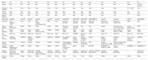
^a Ref represents the domain referenced by the MICS-Asia III project. ^b Standard represents the reference meteorological field provided by the MICS-Asia III project; WRF/NCEP and WRF/MERRA represent the meteorological field of the participating model itself, which was run by WRF and driven by the NCEP
and Modern Era Retrospective-analysis for Research and Applications (MERRA) reanalysis dataset. ^c Boundary conditions of M10 are from MOZART and GOCART (Chin et al., 2002; Horowitz et al., 2003), which provided results for gaseous pollutants and aerosols, respectively.

2.2 Participating models and input data

Table 1 summarizes the specifications of participating CTMs. These models include two versions of CMAQ (v4.7.1 and 5.0.2; Byun and Schere, 2006), the Weather Research and Forecasting model coupled with Chemistry (WRF-Chem; http://www.acd.ucar.edu/wrf-chem, last access: 8 October 2019), the Nested Air Quality Prediction Modeling System (NAQPMS; Li et al., 2007), the Japan Meteorological Agency's (JMA) non-hydrostatic meteorology–chemistry model (NHM-Chem; Kajino et al., 2012), the NASA-Unified Weather Research and Forecasting model (NU-WRF; Tao et al., 2013) and GEOS-Chem (http://acmg.seas.harvard.edu/geos/, last access: 8 October 2019). They have been documented in the scientific literature and have been widely applied in modeling studies of East Asia. Table 1 does not list model names to maintain each model's anonymity. Similar behavior was observed to MICS-Asia II and other model intercomparison projects (e.g., AQME II).

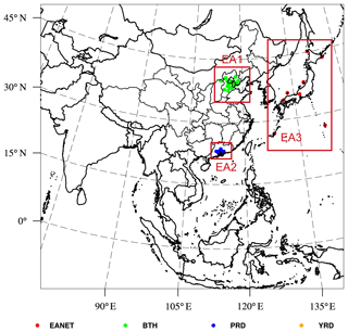
Figure 1 Model domain of models (except M13 and M14) showing the locations of three subregions marked in this study. Also shown are the locations of surface monitoring stations used in this study. The meteorological model used to provide meteorological fields for most models also uses this domain. Note that the domains of M13 and M14 are shown in Fig. 10.

MICS-Asia III participants were provided with a reference meteorological field for the year 2010, generated with the Weather Research and Forecasting model (WRF; version 3.4.1). The domain of the meteorological fields is shown in Fig. 1. WRF v3.4.1 is driven by the final analysis dataset (ds083.2) from the National Centers for Environmental Prediction (NCEP), with a $\mathrm{1}{}^{\circ }\times \mathrm{1}{}^{\circ }$ resolution and a temporal resolution of 6 h. A four-dimensional data assimilation nudging toward the NCEP dataset was performed to increase the accuracy of the WRF. The horizontal model domain of 182×172 grids on a Lambert conformal map projection with a 45 km horizontal resolution is shown in Fig. 1. Vertically, the WRF grid structure consists of 40 layers from the surface to the top of model (10 hPa). Standard meteorological fields were applied by the majority of groups. Several other models were employed to perform simulations using their own meteorological models (e.g., RAMS-CMAQ and GEOS-Chem). WRF-Chem utilized the same model (WRF) as the standard meteorological simulation but considered the feedback of pollutants to the meteorological fields. Consequently, the meteorological fields from this model may be slightly different from the standard. GEOS-Chem is driven by the GEOS-5 assimilated meteorological fields taken from the Goddard Earth Observing System of the NASA Global Modeling Assimilation Office. The meteorological data and CTMs couples varied for each group, likely resulting in a diversified set of model outputs.

MICS-Asia III provided a set of monthly anthropogenic emission inventories for the year 2010 called MIX (Li et al., 2016). MIX is a mosaic of up-to-date regional and national emission inventories that includes Regional Emission inventory in ASia (REAS) version 2.1 for the whole Asian region (Kurokawa et al., 2013), the Multi-resolution Emission Inventory for China (MEIC) developed by Tsinghua University, a high-resolution NH₃ emission inventory by Peking University (Huang et al., 2012), an Indian emission inventory developed by Argonne National Laboratory (ANL India, Lu et al., 2011; Lu and Streets, 2012) and the official Korean emission inventory from the Clean Air Policy Support System (CAPSS; Lee et al., 2011). Biogenic emissions were taken from the Model of Emissions of Gases and Aerosols from Nature (MEGAN); hourly biogenic emissions were obtained for the entire year of 2010 using version 2.04 (Guenther et al., 2006). Biomass burning emissions were processed by regridding the Global Fire Emissions Database version 3 (GFEDv3; 0.5^∘ by 0.5^∘). Volcano SO₂ emissions were provided with a daily temporal resolution by the Asia Center for Air Pollution Research (ACAP). The MICS-Asia III emission group directly prepared a gridded inventory according to the configuration of each CTM. NMVOC emissions were spectated into model-ready inputs for three chemical mechanisms: CBMZ, CB05 and SAPRC-99. Weekly and diurnal profiles were also provided. The standard emission inventory was applied by all models. The majority of models employed the official suggested vertical and time profiles of pollutants from each sector by emission group. M13 and M14 made the projections themselves. More information can be found in Li et al. (2017) and Gao et al. (2018).

MICS-Asia III also provided two sets of chemical concentrations for the top and lateral boundaries of the model domain, which were derived from 3-hourly global model outputs for the year 2010. The global models were run by the University of Tennessee (http://acmg.seas.harvard.edu/geos/, last access: 8 October 2019) and Nagoya University (Sudo et al., 2002). GEOS-Chem was run with a $\mathrm{2.5}{}^{\circ }\times \mathrm{2}{}^{\circ }$ horizontal resolution and 47 vertical layers by the University of Tennessee, and the Chemical AGCM for Study of Atmospheric Environment and Radiative Forcing (CHASER) was run with a $\mathrm{2.8}{}^{\circ }\times \mathrm{2.8}{}^{\circ }$ horizontal resolution with 32 vertical layers by Nagoya University. Some models applied boundary conditions depending on their own past experiences.

2.3 Observational data for O₃

In this study, East Asia was divided into three subregions as shown in Fig. 1. The selection of subregions was based on emission, climate and observation data coverage. The North China Plain (EA1) and the Pearl River Delta (EA2) represent highly industrialized regions of the midlatitudes. EA1 is characterized by a temperate and tropical continental monsoon climate with marked seasonality. EA2 is located in southern China and is less affected by continental air masses. EA3 covers the northwest Pacific and the Sea of Japan and represents the downwind regions of the Asian continent with a marine climate.

Hourly O₃ and NO_x observations for the year 2010 in East Asia were obtained from the CERN, PRD-RAQMN and EANET. The CERN was built by the Institute of Atmospheric Physics, Chinese Academy of Sciences and includes 19 surface stations covering an area of 500km× 500km across the North China Plain (EA1 subregion; Ji et al., 2012). The stations are set up according to United States Environmental Protection Agency method designations. Half of them are remote, rural, suburban and clear urban sites. Nine sites are located within meteorological stations or on campuses of universities in urban regions, with little influence from local sources and sinks. The PRD RAQMN was jointly established by the governments of Guangdong Province and the Hong Kong Special Administrative Region and consists of 16 automatic air quality monitoring stations located across the EA2 subregion (Zhong et al., 2013). Thirteen of these stations are operated by the Environmental Monitoring Centers in Guangdong Province and the other three are located in Hong Kong and are managed by the Hong Kong Environmental Pollution Department. The PRD RAQMN was designed to probe regional air quality, in order to assess the effectiveness of emission reduction measures and to enhance the roles of monitoring networks in characterizing regional air quality and in supporting air quality management. Thus, the sites are rarely influenced by local sources and sinks. The EANET was launched in 1998 to address acid deposition problems in East Asia, following the model of the Cooperative Program for Monitoring and Evaluation of the Long-Range Transmission of Air Pollutants in Europe. In this study, eight remote stations in the northwestern Pacific and Japan (EA3 subregion) were selected to evaluate model performance levels for the downwind regions of the Asian continent (Ban et al., 2016). More information on the EANET can be found at http://www.eanet.asia/ (last access: 8 October 2019). Note that only stations with at least 75 % data validity were chosen. Table S1 in the Supplement provides a detailed site description. Our comparisons of NO_x and VOC emission rates conducted on grids for these stations using 45 and 3 km resolution emission inventories suggest that our selected stations rarely received local emissions.

O₃ was measured by a Thermo Scientific 49i ozone analyzer with UV photometric technology in the CERN network and by a Thermo Scientific 49C ozone analyzer in the PRD-RAQMN and EANET networks. NO_x was measured by a Thermo Scientific 42C $\mathrm{NO}--{\mathrm{NO}}_{\mathrm{2}}--{\mathrm{NO}}_x$ analyzer with chemiluminescence technology at 40 sites in all three networks (CERN, PRD-RAQMN and EANET). NO_x measurements sometimes exhibited biases (especially for stations located far from sources) when using molybdenum converter devices as all nitrogen oxides were measured. This bias was found to be dependent on the chemical conditions. A 1-month continuous measurement with a chemiluminescence analyzer and Aerodyne cavity-attenuated phase shift spectrometer (CAPS) undertaken in August at an urban site in Beijing shows that this bias from the chemiluminescence analyzer is minor when NO₂ concentrations exceed 10–15 ppbv (parts per billion by volume), ranging from 10 % to 30 % under low-NO₂ conditions (<10 ppbv) (Ge et al., 2013). Measurements collected from a rural site in South Korea revealed a similar pattern across all seasons (Jung et al., 2017). These comparisons suggest that observations made using molybdenum converters may overestimate NO₂ by 10 %–20 % for EA1 and EA2 and 30 % for EA3, introducing uncertainties into the NO₂ model evaluation in this study.

Table 2 Statistical analysis for surface O₃ in three subregions over East Asia. R denotes the correlation coefficient, NMB is the normalized mean bias and RMSE is the root-mean-square error (units are ppbv).

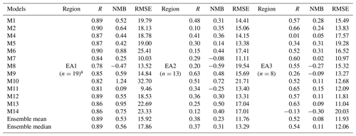
^a n represents the number of observation stations.

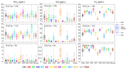
Figure 2 Box plots of the observed and simulated annual NO₂ (a, d, g), NO (b, e, h) and O₃ (c, f, i) frequency distributions determined from 13 models and averaged for stations in EA1, EA2 and EA3 for 2010. n denotes the number of stations. The rectangle represents the interquartile range (25th to 75th percentiles). The asterisk identifies the mean, the continuous horizontal line within the rectangle identifies the median, and whiskers extend between the minimum and maximum values.

3 Model validation and general statistics

3.1 Annual concentrations of surface O₃, nitric oxide (NO) and nitrogen dioxide (NO₂)

Figure 2 provides a concise comparison of model performances for annual O₃, NO and NO₂ for three sub regions of East Asia. A box-and-whisker representation was used to show the frequency distribution of monthly concentrations measured from stations in each subregion. The O₃ normalized mean bias (NMB) and root-mean-square error (RMSE) of the ensemble mean were found to be significantly less than the ensemble median in most cases (Table 2). Therefore, we only present multi-model mean ensemble results (Ense). In general, the majority of the models significantly overestimated annual surface O₃ relative to observations in EA1, EA2 and EA3. Ense overestimated surface O₃ by 10–30 ppbv for these subregions. Ense NO₂ levels closely reflected observations to within ±20 % across all subregions. In EA1 and EA2, Ense NO levels were found to be 5–10 ppbv lower than observations while exhibiting reasonable levels for EA3.

Of the models, M11 (for subregions EA1 and EA2) and M7 (for EA2 and EA3) more closely reflected O₃ observations. M11 simulated O₃ with RMSE values of 9.5 and 13.3 ppbv for EA1 and EA2, respectively (Table 2). The models' performance with respect to simulating O₃ was found to be closely related to their performance for NO₂ and NO. In highly polluted regions (EA1 and EA2), a persistent underestimation of NO was evident across most models. As an interesting phenomenon, we found the models' performance regarding O₃ measurements to vary greatly for EA3, although M8 exhibited consistent performance with respect to NO and NO₂. This finding suggests that O₃ was significantly affected by other factors in addition to local chemistry in EA3. M8 underestimated O₃ and overestimated NO in all subregions by 40 %–50 %. The highest O₃ titration level observed in M8 may have generated lower O₃ levels than those indicated by other models and observations.

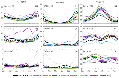
Figure 3 Time series of monthly NO₂, NO and O₃ levels simulated by all models and their ensembles (Ense) in parts per billion by volume (ppbv), averaged over all observed stations across three subregions of East Asia: EA1 (a–c), EA2  (d–f) and EA3 (g–i). Observations are denoted by the solid black line. n represents the number of stations. The gray lines represent NO₂, NO and O₃ levels simulated by models except M1, M2, M4, M6, M11, M12, M13 and M14.

3.2 Monthly variations of surface O₃, NO and NO₂

Figure 3 presents monthly mean concentrations of O₃, NO and NO₂ for the three subregions across East Asia. When two or more observation sites are located in the same model grid, their mean values are used to evaluate model performance. All models captured the observed seasonal cycles of O₃, NO and NO₂ for EA1. From May to September, Ense O₃ was 10–30 ppbv higher than observed values (30 %–70 % of observed values), while Ense NO and NO₂ levels appeared to be consistent with observations with mean biases of <3 ppbv. This finding suggests that an intercomparison of O₃ production efficiency levels per NO_x with observations is needed. For EA2, Ense O₃ values agreed well with observed high autumn O₃ levels but were overestimated by 5–15 ppbv (15 %–60 % of observations) from January to September. This overestimation reached a maximum in March–April (15 ppbv) and led to a spring peak in simulated O₃ values not found in the observations. This overestimation is partly related to the underestimation of NO in the same months, which decreased the titration effect. For NO₂, Ense values agreed well with observed values for June–December, and slightly underestimated observations for January–May. For EA3, the ensemble NO₂ was generally close to observed values (within ±0.5 ppbv). Significant overestimations of O₃ and underestimations of NO were observed from June to October. Similar results were found in MICS-Asia II and in another model intercomparison project of the Task Force on Hemispheric Transport of Air Pollution (TF-HTAP), suggesting that such results may stem from differences in the representation of the dispersion of southwesterly clean marine air masses observed across different metrological fields used in CTMs (Han et al., 2008; Fiore et al., 2009).

For individual models, M11 achieved the highest degree of model reproductivity for monthly mean O₃ levels in EA1. Most of the other models overestimated O₃ by 100 %–200 % for May–October. The largest levels of model bias and inter-model variability for NO and NO₂ appeared in the winter, and likely came from the NO_x vertical diffusion and heterogeneous chemistry (Akimoto et al., 2019). In EA2, M7 seems to have achieved the highest levels of O₃ reproducibility. Most of the models (except for M11 and M12) showed high O₃ concentrations for March–May and September–November. Observed O₃ values show that the highest concentrations appeared from October to November. M11 captured the observed January–May O₃ value due to relatively high NO concentrations. However, NO was overestimated by M11 from May to September, leading to an underestimation of O₃ levels. In EA3, spatially averaged O₃ concentrations often differed by more than 20 ppbv in individual models. The highest levels of inter-model variability in O₃ values appeared from May to October, overestimating O₃ levels relative to observations by 10–40 ppbv. Interestingly, although M8, M9 and M14 exhibited similar magnitudes with observations for June–September, they significantly underestimated observations in other months by 200 %–300 %. A detailed investigation is required in future studies.

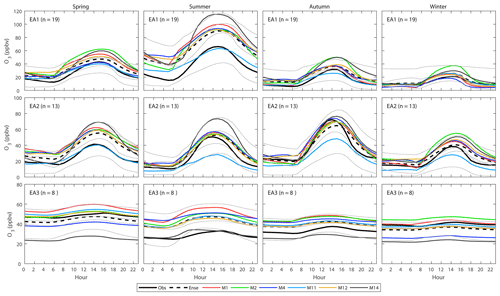
Figure 4 Seasonal mean diurnal cycle of surface O₃, in parts per billion by volume (ppbv), as a function of hours, for all models and their ensembles, averaged across all observed stations in three subregions of East Asia: EA1 (top row), EA2 (middle row) and EA3 (bottom row). Observations are denoted by the thick black line. n represents the number of stations. The gray lines represent O₃ levels simulated by models except M1, M2, M4, M11, M12 and M14. Spring, summer, autumn and winter were defined as March–April–May, June–July–August, September–October–November and December–January–February, respectively.

3.3 Diurnal concentrations of surface O₃

Subregional O₃ diurnal variations are shown in Fig. 4. In general, model results for three subregions exhibited a larger spread with a magnitude of 10–50 ppbv across the diurnal cycle than those observed in Europe and North America (Solazzo et al., 2012). Summer Ense O₃ levels exhibited a systematic pattern of overestimation (20 ppbv) throughout the diurnal cycle in EA1. This indicates that the models had difficulty in estimating summer O₃ levels for the North China Plain. Compared with summer conditions, only a slightly systematic overestimation of Ense O₃ levels was observed for the other seasons (3–5 ppbv). In EA2, Ense O₃ levels generally agreed with summer, autumn and winter observations. In particular, the O₃ maximum occurring at around noon was reasonably reproduced. Only a 3–5 ppbv overestimation was observed from 16:00 to 23:00 LT (local time) and in the early morning (06:00 to 10:00 LT). In the spring, a systematic overestimation of Ense O₃ values was observed across the whole diurnal cycle (5–10 ppbv). In EA3, Ense captured the minor diurnal variations in O₃ across all four seasons, but significantly overestimated observations for the summer and autumn (5–20 ppbv). In the spring and winter, differences between Ense and observations fell within 5 ppbv.

Of all of the models, M11 exhibited the best model performance level with respect to measuring peak daily O₃ concentrations of 60 ppbv from 14:00 to 16:00 LT in EA1, but it still overestimated nighttime O₃ levels by 10 ppbv. Compared with their performance in simulating summer patterns, the models performed significantly better in simulating winter conditions due to the weak intensity of photochemical reactions except in the case of M2, M10 and M8. Differences between observations and most simulations for both the nighttime and daytime fell within 5 ppbv. These differences in the models' performances between the summer and winter imply that the variety of chemistry parameterizations applied to different models partly explain the inter-model variability of simulated O₃ levels in EA1 (North China Plain). For EA2, the majority of models agreed well with diurnal variations occurring in the summer and autumn. However, most models exhibited a tendency to overestimate the O₃ concentrations for both the daytime and nighttime in the spring. The overestimated magnitudes exceeded 10 ppbv and 25 ppbv (of observed values of 20–35 ppbv) for the nighttime and daytime, respectively. M11 reproduced observed O₃ levels for the spring but underestimated O₃ levels for the summer and autumn. For EA3, significant levels of inter-model variability persisted throughout the year. Amplitudes of inter-model variability except for those of M8 and M14 reached approximately 20 ppbv and 10 ppbv in the spring–summer and autumn–winter, respectively. M8 and M14 generated the lowest O₃ values of the models for the whole year.

3.4 Error statistics on surface concentrations

In this section, we present statistics on the models' performance based on monthly values. Values are calculated using the equations shown in Appendix A. On a yearly basis, all models showed the highest (0.8–0.9) and lowest (0.1–0.6) correlation coefficients for O₃ for EA1 and EA2, respectively (Table 2). High correlations were found in EA1 mainly because the summer-maximum and winter-minimum seasonal cycles are typical of polluted regions represented in all of the participating models. In general, Ense performed better than the individual models in representing NO₂ for East Asia, reproducing the observed seasonal cycles and magnitudes. However, Ense did not always exhibit superior performance in simulating O₃ levels over individual models for East Asia, which stands in contrast with its performance for Europe (Table 2). M7 and M11 agreed well with observations for EA1 and EA2, whereas Ense tended to overestimate O₃ concentrations for May–September in EA1 and for January–September in EA2. Loon et al. (2007) indicated that Ense exhibits superior performance only when the spread of ensemble-model values is representative of O₃ uncertainty. This indicates that most models do not reflect this uncertainty or miss key processes of MICS-Asia III.

Considerable overestimations made by most of the models for May–September led to high NMB (0.25–1.25) and RMSE (10–33 ppbv) values for EA1. M11 generated the lowest NMB (0.09) and RMSE (9.46 ppbv) values of the examined models. For EA2, M9 and M10 generated stronger correlations than the other models. However, their corresponding NMB and RMSE values were also the highest. These findings imply that systematic model biases are present in these two models. M7 exhibited lower NMB and RMSE values than the other models, but its correlation was measured as only 0.29. For EA3, correlations exhibited the largest degree of inter-model variability across all subregions, ranging from −0.13 to 0.65. M7 generated the lowest NMB and RMSE, likely due to the canceling effect of its overestimation for the summer and underestimation for other seasons (Fig. 3).

Table 3 Statistical analysis for surface NO in three subregions over East Asia. R denotes the correlation coefficient, NMB is the normalized mean bias and RMSE is the root-mean-square error (units are ppbv).

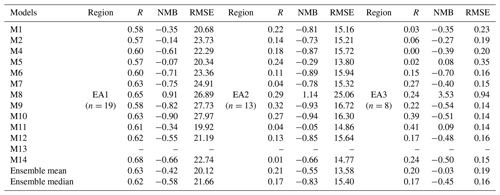
^a n represents the number of observation stations.

Table 4 Statistical analysis for surface NO₂ in three subregions over East Asia. R denotes the correlation coefficient, NMB is the normalized mean bias and RMSE is the root-mean-square error (units are ppbv).

^a n represents the number of observation stations.

For NO, model correlations for EA1 ranged from 0.57 to 0.68, showing that all of the models effectively reproduced the spatial variability in NO for this subregion (Table 3). NMBs indicated that underestimations by the models except in the case of M8, mostly occurred for the winter. This underestimation can be partly attributed to the coarse model horizontal resolution (45 km) used in MICS-Asia III, which hardly reproduced concentrations of short-lived species (e.g., NO). In contrast with most of the other models, M8 overestimated NO concentrations for all three subregions. It is noted that NO observations for EA3 were too low (<0.3 ppbv) to be discussed in this study.

Table 4 shows statistics regarding the models' performance in measuring NO₂ levels. In general, most of the models performed better with respect to representing NO₂ than O₃ and NO for EA1. NMBs ranged from −0.28 to 0.32, falling far below those measured for O₃ (0.48–1.25). Correlations of 0.54–0.66 were recorded, implying the models' reliable performance in reproducing spatial and monthly variability of NO₂ for EA1. Similar to those for O₃ and NO, correlation coefficients for NO₂ in EA2 remained low. Thus, a dedicated investigation of O₃, NO and NO₂ levels in EA2 is urgently needed, but falls beyond the scope of this study. In EA3, correlation coefficients ranged from 0.43- to 0.72. NMBs and RMSEs, except for those of M8, ranged from −0.23 to 0.46 and 0.90 to 1.79 ppbv, respectively.

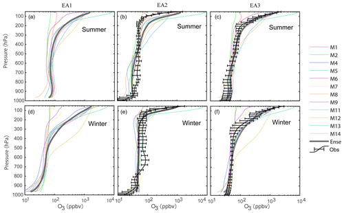
Figure 5 Simulated O₃ profiles for the summer (June–July–August) and winter (December–January–February) of 2010, averaged over all observed stations across three subregions of East Asia: EA1 (a, d), EA2 (b, e) and EA3: (c, f). Ozonesonde data for 2010 were taken from the World Ozone and Ultraviolet Radiation Data Centre (WOUDC) database.

3.5 Vertical profiles of O₃

Figure 5 shows the vertical profiles of the observed and simulated O₃ levels for East Asia for the summer and winter. Ensemble means (Ense) showed underestimations and overestimations of EA2 O₃ levels for the middle (500–800 hPa) and lower (below 900 hPa) troposphere, respectively. In the winter, underestimations extended to 200 hPa. Magnitudes of underestimations and overestimations reached 10–40 and 10–20 ppbv, respectively. For EA3, Ense reproduced the vertical structure of O₃ for both the summer and winter. An overestimation of the region below 800 hPa, with a magnitude of 10–20 ppbv, was observed for the summer.

High levels of inter-model variability in O₃ exceeding 300 hPa was evident across all subregions, which was attributable to the varied top boundary conditions applied by the models. However, this considerable variability was not transmitted to the middle troposphere (400–600 hPa), in which O₃ concentrations were consistent across the models. In the lower troposphere, a minor level of inter-model variability below 900 hPa appeared in the winter in three subregions, and slowly decreased with height. Mean standard deviations (SD) of models below 900 hPa were recorded as 7.6 6.9 and 6.0 ppbv for EA1, EA2 and EA3, respectively, covering 18.3 %, 15.0 % and 15.4 % of mean O₃ concentrations. In the 700–900 hPa region, SD levels decreased to 5.4, 4.4 and 4.8 ppbv for EA1, EA2 and EA3, representing 12.2 %, 9.4 % and 10.8 % of mean O₃ concentrations, respectively.

In the lower troposphere, inter-model variability in the summer was generally higher than that in the winter. In polluted regions (EA1), SD levels reached 16.3 ppbv (20.8 % of mean concentrations) in the summer, greatly exceeding those in winter (6.2 ppbv, 15.2 %). Various vertical structures of O₃ were found below 700 hPa in summer. O₃ concentrations slowly increased with height in M8 and M11, but they mixed well in the planetary boundary layer (PBL) and decreased from 800 to 700 hPa in the other models. Akimoto et al. (2019) found that the parameterization on downward O₃ transport from the upper boundary layer contributed considerably to discrepancies between M1, M6 and M11. In EA2, vertical structures of O₃ among models were found to be consistent, but concentrations differed more than those in EA1. SD values covered 22 % of mean concentrations.

Figure 6 Ensemble mean seasonal surface O₃ concentrations and CV values for different seasons. CV is defined as the standard deviation of the modeled fields divided by the average for different seasons.

4 Multi-model ensemble O₃ and comparison with MICS-Asia II

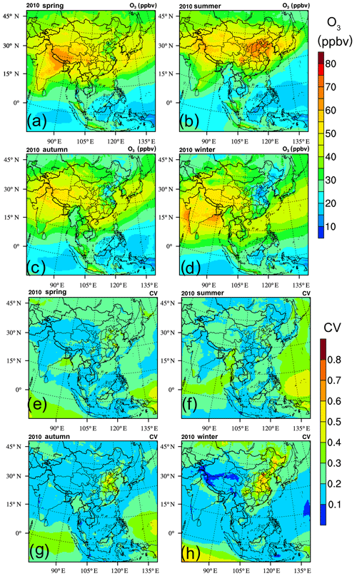
4.1 Spatial distributions of single-model and multi-model ensemble O₃

Figure 6 shows the spatial distributions of MICS-Asia III ensemble mean surface O₃ values (Ense) and the coefficient of variation (CV). The CV is defined as the standard deviation of the modeled O₃ divided by the average. The larger the CV value, the lower the degree of consistency among the models. For the summer, Ense predicted an elevated O₃ concentration belt in the midlatitudes (30–45^∘ N). A region of O₃ in excess of 60 ppbv stretched across the North China Plain and East China Sea, far exceeding MICS-Asia II (45–50 ppbv) values for 2001 (Han et al., 2008). In other seasons, the O₃ distribution showed higher O₃ over the ocean than in eastern China, reflecting O₃ titration from high NO_x emissions. Due to the stratospheric injection, surface O₃ over the Tibetan Plateau remained at high levels throughout the year, ranging from 50 to 65 ppbv. The seasonal cycle of surface O₃ levels determined from Ense via MICS-Asia III agreed with that observed from MICS-Asia II, but O₃ levels in polluted regions were higher (Han et al., 2008).

Figure 7 Surface O₃ spatial distribution derived from 13 models for summer 2010 (units in ppbv).

The CV ranged from 0.1 to 0.6 in East Asia. The high values were found in EA1 in the winter. These high values in the low-latitude western Pacific (10^∘ S–15^∘ N) and Indian oceans were likely caused by the treatment of lateral boundaries in the models. For MICS-Asia III, M7, M8 and M9 employed the default model configurations, and the others employed outputs of the GEOS-Chem/CHASER/MOZART-GOCART global model. Compared with those of MICS-Asia II, CVs for the Asian continent except for the winter remained at similar levels in this study (0.1–0.3) (Carmichael et al., 2008).

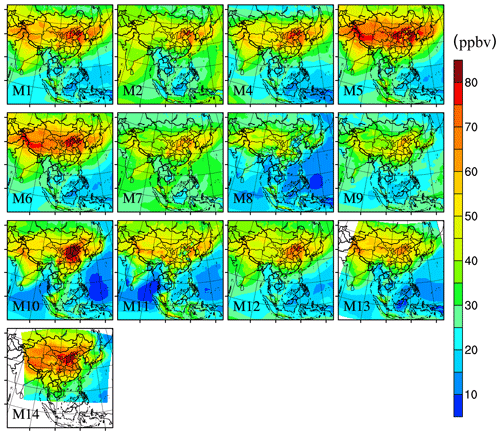
Although all of the models similarly predicted the emergence of an elevated summer O₃ concentration belt in the midlatitudes (30–45^∘ N), the magnitudes of enhanced O₃ levels varied between the models (Fig. 7). M5 predicted the highest O₃ concentrations of 60–90 ppbv for the North China Plain (EA1) and for its outflow pathways including the Bohai Sea, East China Sea, Korea, Japan and the Sea of Japan (locations are shown in Fig. S1 in the Supplement), whereas M8 predicted the lowest levels of 35–50 ppbv. Overhangs of 30 ppbv contour lines extending into the northwestern Pacific along the Asian continent outflow plume differed considerably between the models. A plume of 30 ppbv, or higher O₃ levels, was simulated in M1–M6, M13 and M14, reaching further south and east of Japan (135^∘ E, 20^∘ N), than those of M8, M10 and M11 (120^∘ E, 30^∘ N). From MICS-Asia II and HTAP, differences in the frequency of marine air masses from the western Pacific Ocean were thought to be a possible cause of O₃ discrepancies observed over oceans between the models due to different meteorological drivers (Han et al., 2008). For MICS-Asia III, wind fields employed by the models were similar due to the use of the same or similar meteorological fields (Fig. S2). These inconsistencies between the models resulted from the combined effects of a series of factors, including the diversity of the condensed gas chemical mechanism and heterogeneous chemistry. Li et al. (2016) found chemical production to be the dominant controlling factor of O₃ along outflow pathways near the North China Plain in the summer rather than lateral and top boundary conditions. Impacts of aerosols on O₃ in these regions have frequently been reported (e.g., Olson et al., 1997 and Li et al., 2018) to alter photolysis rates and heterogeneous chemistry patterns. Detailed comparisons of parameterizations of these processes in models are needed in future inter-model comparison projects focused on Asia.

In the winter, distribution patterns of O₃ were quite similar between the models with high concentrations observed over parts of western China, northeastern India and the western Pacific from the East China Sea to southern Japan (Fig. S3). In the spring and autumn (Figs. S4 and S5), O₃ concentrations were generally higher than they were in the winter across the whole model domain due to the enhancement of solar radiation or stratosphere–troposphere exchange fluxes of O₃. All of the models exhibited an enhancement of O₃ levels over southern Tibet, northeastern India and the western Pacific, generally echoing patterns observed in the winter. Increases of O₃ further north in Japan were comparable with winter.

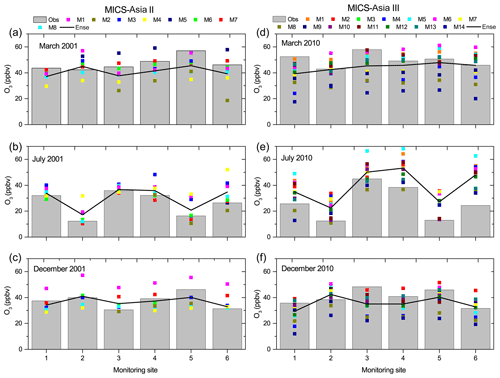
Figure 8 Modeled and observed monthly mean concentrations of O₃ for EANET sites in phases II (a–c) and III (d–f) of the MICS-Asia project. The solid line represents the ensemble mean. Note that MICS-Asia II and III data refer to March, July and December of 2001 and 2010, respectively. IDs of the monitoring sites denote the following: 1 – Rishiri (45.12^∘ N, 141.23^∘ E), 2 – Ogasawara (27.83^∘ N, 142.22^∘ E), 3 – Sado-seki (38.23^∘ N, 138.4^∘ E), 4 – Oki (36.28^∘ N, 133.18^∘ E), 5 – Hedo (26.85^∘ N, 128.25^∘ E) and 6 – Banryu (34.67^∘ N, 131.80^∘ E)

4.2 Comparison with MICS-Asia II

From MICS-Asia II, model evaluation of O₃ was conducted on sites in the western Pacific. Figure 8 presents the simulated and observed surface O₃ levels at these monitoring sites derived from phases II and III of the MICS-Asia project. Note that different models were employed in the two phases. In general, most of the models captured distributions of O₃ mixing ratios at most sites in both MICS-Asia II and III. Ense results were consistent for March and December of 2001 and 2010. Underestimations of O₃ levels in March at the Japanese sites (Site 4 – Oki, Site 5 – Hedo and Site 6 – Banryu) in Phase II were largely remedied in Phase III. However, surface O₃ observed in western Japan (Site 4 – Oki, Site 5 – Hedo and Site 6 – Banryu) were severely overestimated in July 2010 by 10–30 ppbv. This overestimation was not found in Phase II, for which differences from observations were valued at approximately 5 ppbv. Rural sites in western Japan are located in the upwind regions of Japanese domestic emissions, and are subjected to the impacts of Asian continent outflows. Overestimated O₃ values for the North China Plain (EA1) in Phase III contributed considerably to enhanced concentrations simulated for western Japanese sites in July 2010. This indicates that transboundary transport from the Asian continent according to MICS-Asia III was likely overestimated relative to that measured from MICS-Asia II.

5 Discussions

In reference to MICS-Asia II, Han et al. (2008) hypothesized that variations in meteorological fields, dry deposition, PBL, model treatments of chemistry and other physical processes contributed to model biases in relation to observations and inter-model variability. Quantifying the contributions of these processes can help explain model biases through sensitivity simulations. However, this task comes with tremendous computational costs when applied to 14 models. The qualitative analysis of potential causes of these processes based on comparisons of models and observations is essential to selecting sensitivity simulating scenarios for the next phase of MICS-Asia. In MICS-Asia III, common input data (emission and meteorology) were effectively used in this qualitative analysis based on model parameterizations. We evaluated the models on dry deposition, PBL and chemistry by collecting their observations (dry deposition velocity and PBL height). This work was not conducted under MICS-Asia II and is intended to help model developers improve model performance for East Asia.

5.1 Dry deposition

Previous studies show that dry deposition processes serve as the key net sink of O₃, accounting for roughly 25 % of the total O₃ removed from the troposphere (Lelieveld and Dentener, 2000). The uncertainty of dry deposition in CTMs is still high because many processes are heavily parameterized in models (Hardacre et al., 2015). In this study, the simulated dry deposition velocities of O₃ were compared. Simulated deposition velocities were calculated from Eq. (1):

$$\begin{array}{}\text{(1)}& V_{\mathrm{d}}=F/C,\end{array}$$

where F and C represent the simulated dry deposition flux and surface O₃ concentrations, respectively. We determined spatial mean dry deposition velocities from stations in each subregion.

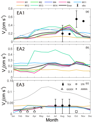
Figure 9 Simulated and observed monthly O₃ dry deposition velocities (V_d) for M1, M2, M4, M6, M11, M12, M13 and M14 for three subregions of East Asia: EA1 (a), EA3 (b) and EA3 (c). TEX, STR, GGSEX and AMMA denote observations for TexAQS06 (7 July–12 September 2006; northwestern Gulf of Mexico), STRATUS06 (9–27 October 2006; the persistent stratus cloud region off the coast of Chile in the eastern Pacific Ocean), GasEx08 (29 February–11 April 2008; the Southern Ocean), and AMMA08 (27 April–18 May 2008; the southern and northern Atlantic Ocean). Observational data were taken from Sorimachi et al. (2003), Pan et al. (2010) and Helmig et al. (2012).

Figure 9 presents the simulated and observed monthly spatial mean dry deposition velocities of O₃. For EA1, ensemble mean values overestimated observed dry deposition velocities of O₃ (v_d) for August–September, but they still fell within the range of the observed standard deviation. This shows that factors other than dry deposition could play important roles in overestimations of August–September O₃ values in EA1. In October–November, simulated v_d apparently underestimated observations by 30 %–50 %. Among the models, the lower dry deposition velocities in May–July for M1, M2, M4 and M6 than that of M11 partly explained the higher May–July surface O₃ from those simulations than the value from in M11. However, M13 and M14 still produced high O₃ concentrations in May–September, although their dry deposition velocities were similar to that of M11 (Fig. 3). Notably, our observations were made on grassland, which covers ∼20 % of the land area in EA1. There are few v_d observations on agriculture crops (50 % of the land area) in North China. Hardacre et al. (2015) reported O₃ dry deposition measurements on crops in Europe and simulated O₃ dry deposition in 15 global models. Both observations and simulations showed that O₃ dry deposition velocities on the agriculture crop class were quite similar to those of grassland, displaying that uncertainties related to the representativeness of measurement sites used in this study did not affect our conclusions.

For EA2, similar features to those of EA1 were found. M1, M2, M4 and M6 were quite consistent with each other, with a seasonal cycle and a spring minimum. M11, M12 and M14 show no obvious signs of seasonal variability with a magnitude of 0.1–0.2 cm s⁻¹. Seasonal patterns in M13 are considerably different from those of the other models, exhibiting a maximum in April–September with higher dry deposition velocities (0.5 cm s⁻¹). The performance of the models for dry deposition velocities was not always consistent with O₃ concentrations. For example, O₃ concentrations in M13 remained high under higher dry deposition velocities.

In EA3, most stations were located at remote oceanic sites, and few dry deposition observations were made. Thus, we collected observations from other oceanic sites to evaluate model performance (Helmig et al., 2012). Ense values for v_d agreed reasonably well with observations (Fig. 9). Both observations and simulated v_d values showed a July–September maximum with a magnitude of 0.02–0.03 cm s⁻¹. Park et al. (2014) found surface O₃ levels in EA3 to be more sensitive to dry deposition parameterization schemes in CTMs. O₃ measured from oceans differed by 5–15 ppbv in East Asia due to the use of various dry deposition parameterization schemes. Thus, more observations are needed over oceans in EA3 to mitigate O₃ simulation uncertainties.

Figure 10 Scatterplots for monthly daytime (08:00–20:00 LT) surface NO_x and O₃ for each station in EA1 (red), EA2 (green) and EA3 (blue) in May–October, for observations (Obs) and models. Also shown are the linear regression equations for NO_x and O₃ in EA1 (red) and EA2 (green).

5.2 Relationships between surface NO_x and O₃

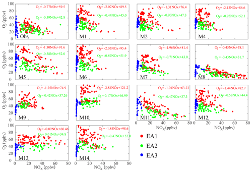
In general, surface O₃ mainly comes from photochemistry processes involving NO_x and VOCs in polluted regions. Examining O₃−NO_x relationships is effectual to investigating sources of inter-model variability and model errors concerning O₃ chemistry in East Asia. Fig. 10 presents O₃ concentrations as a function of NO_x in May–September based on the monthly daytime (08:00–20:00 LT) mean observed and simulated results for the stations shown in Fig. 1.

For EA1 (North China Plain), observations clearly show that O₃ concentrations decreased with an increase in the NO_x concentrations. O₃ concentrations mostly remained at high levels (40–60 ppbv) when NO_x was less than 20 ppbv. The slope and intercept of the regression line between observed O₃ and NO_x were measured as −0.77 ppbv ppbv⁻¹ and 59.5 ppbv, respectively. Among the models, M11 results were in relative agreement with observations. The slope and intercept (−1.01  ppbv ppbv⁻¹, 63.23 ppbv) reflected the observations. The other models showed a higher degree of model bias and inter-model variability in relationships between O₃ and NO_x. Their slopes mostly ranged from −1.25 to −2.13 ppbv ppbv⁻¹, amounting to 1.3–2.8 times the observed slope. Their intercepts were 74.9–121.2 ppbv, far exceeding observations (59.5 ppbv). Akimoto et al. (2019) calculated the net photochemical production of M1, M6 and M11 and found that weak net chemical production in M11 was mostly responsible for low O₃ compared with those in M1 and M6. This finding is consistent with the low slope in M11. To reduce the impact of O₃ buildup and transport due to NO_x consumption, the relationship between O_x (NO₂+O₃) and NO_x was compared (Fig. S7). Observed O_x increases with an increase in NO_x levels, with a coefficient of determination (R²) of 0.61. Most of the models (except for M8, M11 and M13) failed to reproduced observed positive correlations between O_x and NO_x, and their R² only ranged from 0.01 to 0.08. The slope, intercept and R² of M8 and M11 were in relative agreement with observations.

For EA2, all models reproduced observed key patterns in which O_x positively correlated with NO_x. For O₃−NO_x relationships, M1, M2, M4 and M6 reproduced observed O₃ levels under low-NO_x conditions (<30 ppbv) but failed to capture low O₃ under high-NO_x conditions (30–40 ppbv), accounting for overestimations of these models for O₃ in May–September. By contrast, M8 and M11 produced excessively high NO_x values, resulting in their underestimations of O₃ values. For M13 and M14, O₃ concentrations were nearly constant at all levels of NO_x. O₃ was positively correlated with NO_x in M9 and M10, which stands in contrast with observations. This finding suggests that more attention is required when using M9, M10, M13 and M14.

Stations in EA3 are mostly located over clean oceans or islands. NO_x concentrations were less than 3 ppbv, showing that local chemistry was not a key factor shaping O₃ formation. Thus, we did not examine the simulated O₃–NO_x relationship further.

5.3 Other factors

Previous studies show that O₃ precursors are mostly constrained within the boundary layer (Quan et al., 2013). The planetary boundary layer height (PBLH) model evaluation is essential for the interpretation of model biases with observations. Unfortunately, this evaluation was not applied in MICS-Asia II. In 2016, Guo et al. (2016) calculated the PBLH using the bulk Richardson number (Ri) method from the radiosonde network of the L-band sounding system of the China Meteorological Administration (Vogelezang and Holtslag, 1996). The system provides fine-resolution profiles of temperature, pressure, relative humidity, wind speed and direction. In MICS-Asia III, all selected models exhibited the spring-maximum and winter-minimum seasonal cycle for EA1 (Fig. S6), capturing the main climatological pattern of PBLH observations (Guo et al., 2016). The Ense on the PBLH only overestimated radiosonde measurements by 100–200 m (∼10–15 %), likely due to sampling bias between the models and measurements. The simulation was recorded as the mean value of 12 h (08:00–20:00 LT), while the average of the measurements was calculated based on a 3 h period (08:00, 14:00 and 20:00 LT). For EA2, the observed PBLH did not vary as much as that for EA1, and differences between seasons ranged within 100 m. This pattern was captured by the models. As was observed from EA1, the simulated PBLH for EA2 exceeded the measurements by 100–200 m. Few measurements of remote oceanic sites in East Asia were collected. Thus, we compared simulations with European Centre for Medium-Range Weather Forecasts Reanalysis data (von Engeln et al., 2013). Both showed a winter-maximum pattern for PBLH.

6 Summary

Under the MICS-Asia III framework, the evaluation and intercomparison of 13 CTMs were conducted using a wide variety of observations covering two Chinese industrialized regions and the western Pacific, using continuous simulations for 2010 with a focus on O₃, NO and NO₂. In particular, surface O₃ levels in China, which were neglected in previous model intercomparison projects, were evaluated. Considerable levels of inter-model variability in O₃ were observed across all subregions of East Asia, with model concentrations varying by factors of 2 to 3 between different models.

A model ensemble was produced and evaluated. In general, the model ensemble captured key patterns of monthly and diurnal O₃, NO and NO₂ in the North China Plain and on the western Pacific Rim. It failed to capture the observed seasonal cycle of O₃ for the Pearl River Delta. For the North China Plain and the western Pacific Rim, the model ensemble severely overestimated surface O₃ levels for May–September by 10–30 ppbv. This overestimation systematically appeared at both daytime and nighttime. Similarly, the model ensemble tended to overestimate spring daytime and nighttime O₃ concentrations for the Pearl River Delta. Compared with MICS-Asia II, MICS-Asia III was less prone to underestimating surface O₃ in March for Japanese sites. However, it predicted excessively high surface O₃ concentrations for western Japan in July, which was not the case for MICS-Asia II. In term of O₃ soundings, the ensemble model used in this study reproduced the vertical structure in the western Pacific, but overestimated O₃ below 800 hPa in the summer. For the industrialized Pearl River Delta, the ensemble average presented an overestimation of O₃ levels for the lower troposphere and underestimations in the middle troposphere. We find that the ensemble average of 13 models for O₃ did not always perform better than individual models for East Asia in contrast with their performance for Europe. This suggest that the spread of ensemble-model values does not represent all uncertainties in O₃ levels or that most MICS-Asia III models missed key processes. In contrast to performance levels for O₃, Ense performed better than individual models for NO₂ in East Asia.

MICS-Asia II outlines potential causes of variability among models. Quantifying the contributions of these processes to O₃ concentrations serves as an effective way to explain model biases through sensitivity simulations. However, this would incur tremendous computational costs when applied to 14 models. In this study, we conducted a qualitative analysis of potential causes by comparing models and observations for these processes to identify sensitivity simulating scenarios for the next phase of MICS-Asia. Our comparisons show that the ensemble model overestimated observed dry deposition velocities of O₃ for August–September in the North China Plain, displaying that other factors rather than dry deposition may contribute to the overestimation of the simulated O₃ concentrations in the summer. For the western Pacific, simulated v_d values agreed reasonably well with observations. Photochemical treatment in models may contribute to O₃ overestimations in the North China Plain. The models studied captured the major climatological pattern of PBLH observations for three subregions of East Asia. More evaluations of turbulent kinetic energy in the PBL are needed to assess vertical mixing in future studies.

Appendix A: Statistical measures

Defining y_ij and Obs_ij (modeled and observed, respectively) of the ith monthly concentrations of air pollutants at the jth station, with respective mean values of $\stackrel{\mathrm{‾}}{y}$ and $\stackrel{\mathrm{‾}}{\mathrm{Obs}}$. m and n represent the number of stations and months, respectively.

A1 Correlation coefficient (R)

$$\begin{array}{}\text{(A1)}& R={\displaystyle \frac{\sum _{j=\mathrm{1}}^m\sum _{i=\mathrm{1}}^n(y_{ij}-\stackrel{\mathrm{‾}}{y})({\text{obs}}_{ij}-\stackrel{\mathrm{‾}}{\text{obs}})}{\sum _{j=\mathrm{1}}^m\sum _{i=\mathrm{1}}^n(y_{ij}-\stackrel{\mathrm{‾}}{y}{)}^{\mathrm{2}}\sum _{j=\mathrm{1}}^m\sum _{i=\mathrm{1}}^n({\text{Obs}}_{ij}-\stackrel{\mathrm{‾}}{\text{Obs}}{)}^{\mathrm{2}}}}\end{array}$$

A2 Root-mean-square error (RMSE)

$$\begin{array}{}\text{(A2)}& \mathrm{RMSE}=\sqrt{{\displaystyle \frac{\sum _{j=\mathrm{1}}^m{\sum }_i^n(y_{ij}-{\mathrm{Obs}}_{ij}{)}^{\mathrm{2}}}{n}}}\end{array}$$

A3 Normalized mean bias (NMB)

$$\begin{array}{}\text{(A3)}& \mathrm{NMB}={\displaystyle \frac{\sum _{j=\mathrm{1}}^m\sum _{i=\mathrm{1}}^n(y_{ij}-{\mathrm{Obs}}_{ij})}{n\times \stackrel{\mathrm{‾}}{y}\times \stackrel{\mathrm{‾}}{\text{Obs}}}}\end{array}$$