the Creative Commons Attribution 4.0 License.
the Creative Commons Attribution 4.0 License.
 | 13 Sep 2019
The effect of atmospheric nudging on the stratospheric residual circulation in chemistry–climate models
Amanda C. Maycock
Martyn P. Chipperfield
Sandip Dhomse
Hella Garny
Douglas Kinnison
Hideharu Akiyoshi
Makoto Deushi
Rolando R. Garcia
Patrick Jöckel
Oliver Kirner
Giovanni Pitari
David A. Plummer
Laura Revell
Eugene Rozanov
Andrea Stenke
Taichu Y. Tanaka
Daniele Visioni
Yousuke Yamashita
We perform the first multi-model intercomparison of the impact of nudged meteorology on the stratospheric residual circulation using hindcast simulations from the Chemistry–Climate Model Initiative (CCMI). We examine simulations over the period 1980–2009 from seven models in which the meteorological fields are nudged towards a reanalysis dataset and compare these with their equivalent free-running simulations and the reanalyses themselves. We show that for the current implementations, nudging meteorology does not constrain the mean strength of the stratospheric residual circulation and that the inter-model spread is similar, or even larger, than in the free-running simulations. The nudged models generally show slightly stronger upwelling in the tropical lower stratosphere compared to the free-running versions and exhibit marked differences compared to the directly estimated residual circulation from the reanalysis dataset they are nudged towards. Downward control calculations applied to the nudged simulations reveal substantial differences between the climatological lower-stratospheric tropical upward mass flux (TUMF) computed from the modelled wave forcing and that calculated directly from the residual circulation. This explicitly shows that nudging decouples the wave forcing and the residual circulation so that the divergence of the angular momentum flux due to the mean motion is not balanced by eddy motions, as would typically be expected in the time mean. Overall, nudging meteorological fields leads to increased inter-model spread for most of the measures of the mean climatological stratospheric residual circulation assessed in this study. In contrast, the nudged simulations show a high degree of consistency in the inter-annual variability in the TUMF in the lower stratosphere, which is primarily related to the contribution to variability from the resolved wave forcing. The more consistent inter-annual variability in TUMF in the nudged models also compares more closely with the variability found in the reanalyses, particularly in boreal winter. We apply a multiple linear regression (MLR) model to separate the drivers of inter-annual and long-term variations in the simulated TUMF; this explains up to ∼75 % of the variance in TUMF in the nudged simulations. The MLR model reveals a statistically significant positive trend in TUMF for most models over the period 1980–2009. The TUMF trend magnitude is generally larger in the nudged models compared to their free-running counterparts, but the intermodel range of trends doubles from around a factor of 2 to a factor of 4 due to nudging. Furthermore, the nudged models generally do not match the TUMF trends in the reanalysis they are nudged towards for trends over different periods in the interval 1980–2009. Hence, we conclude that nudging does not strongly constrain long-term trends simulated by the chemistry–climate model (CCM) in the residual circulation. Our findings show that while nudged simulations may, by construction, produce accurate temperatures and realistic representations of fast horizontal transport, this is not typically the case for the slower zonal mean vertical transport in the stratosphere. Consequently, caution is required when using nudged simulations to interpret the behaviour of stratospheric tracers that are affected by the residual circulation.
- Article
(11935 KB) - Full-text XML
-
Supplement
(2633 KB) - BibTeX
- EndNote


The Brewer–Dobson circulation (BDC) is characterized by upwelling of air in the tropics, poleward flow in the stratosphere, and downwelling at mid-latitudes and high latitudes. The circulation can be separated into two branches: the shallow branch in the lower stratosphere and the deep branch in the middle stratosphere and upper stratosphere (Plumb, 2002; Birner and Bönisch, 2011). The BDC affects the distribution of trace species in the stratosphere, such as ozone, and its strength partly determines the lifetimes of long-lived gases such as chlorofluorocarbons (CFCs; Butchart and Scaife, 2001). It also determines stratosphere-to-troposphere exchange of ozone (Hegglin and Shepherd, 2009), which is important for the tropospheric ozone budget (Wild, 2007). In the tropical lower stratosphere, where the photochemical lifetime of ozone is long, variations and trends in the strength of the BDC are the main drivers of ozone within the annual cycle (Weber et al., 2011) for inter-annual and longer-term variability (Randel and Thompson, 2011) and in response to climate change (e.g. Keeble et al., 2017). Here we focus on the advective part of the BDC, or the residual circulation, which is driven by wave breaking in the stratosphere from planetary-scale Rossby waves and gravity waves (Holton et al., 1995). It is important to note that the overall tracer transport in the stratosphere is also affected by turbulent eddy mixing, which has been evaluated separately in previous studies (Garny et al., 2014; Ploeger et al., 2015a, b; Dietmüller et al., 2018; Eichinger et al., 2019; Šácha et al., 2019). The residual circulation is commonly evaluated in model (Butchart et al., 2010, 2011) and reanalysis (Abalos et al., 2015; Kobayashi and Iwasaki, 2016) studies using the transformed Eulerian mean circulation (TEM; Andrews and McIntyre, 2002, 1978; Andrews et al., 1987).
Past studies have shown substantial spread across chemistry–climate models (CCMs) in the mean strength of the residual circulation (e.g. Butchart et al., 2010). Nevertheless, CCMs consistently simulate a long-term strengthening of the residual circulation with an increase of ∼ 2 % per decade (e.g. Butchart et al., 2010; Hardiman et al., 2014), though there are differences across models in the relative contribution to trends from resolved and parameterized wave forcing. Reanalysis datasets also suggest a strengthening of the residual circulation over the past few decades of the order of 2 % per decade to 5 % per decade (Abalos et al., 2015; Miyazaki et al., 2016), apart from one dataset (ERA-Interim – ERA-I) which shows a weakening of the deep branch of the BDC (Seviour et al., 2012; Abalos et al., 2015). However, reanalyses are subject to multiple caveats, particularly in their suitability for trend studies, and there can be substantial differences in residual circulation trends calculated from the same reanalysis using different methods (Abalos et al., 2015).
Given the limitations of reanalyses, evaluating the fidelity of model estimates of residual circulation variability and trends is challenging, since there are no direct measurements of the residual circulation. The only direct estimates of the stratospheric mass circulation come from tracer measurements, which can be used to calculate the stratospheric age of air (AoA; Kida, 1983; Schmidt and Khedim, 1991; Waugh and Hall, 2002). The AoA represents the combined effects of advection and mixing processes and as such cannot be directly related to the residual circulation. While progress has been made in separating the relative effects of advection and mixing for the AoA calculated from models (Garny et al., 2014; Dietmüller et al., 2018; Eichinger et al., 2019; Šácha et al., 2019) from Lagrangian models driven by reanalysis data (Ploeger et al., 2015a, b, 2019; Ploeger and Birner, 2016), and comparing the effects in both CCMs and Lagrangian models (Dietmüller et al., 2017), this is more difficult to achieve in observations. Engel et al. (2009) used balloon-borne measurements of stratospheric trace gases and found a statistically non-significant increase in the AoA in the middle stratosphere at northern mid-latitudes; this has been corroborated in a more recent study using longer measurement records at two mid-latitude sites in the Northern Hemisphere (NH; Engel et al., 2017). It has been hypothesized based on analyses of recent satellite tracer datasets, which have greater spatial and temporal coverage, that subtropical AoA trends can be explained by a weakening of the mixing barriers at the edge of the tropical pipe (Neu and Plumb, 1999) that is masking the effects of an increase in tropical upwelling on the AoA (Stiller et al., 2012; Haenel et al., 2015). In contrast with AoA trends derived from observations, CCMs forced with observed sea-surface temperatures (SSTs), greenhouse gases, and ozone-depleting substances (ODSs) show a decrease in the AoA throughout the stratosphere (Karpechko and Maycock, 2018; Li et al., 2018; Morgenstern et al., 2018; Abalos et al., 2019; Polvani et al., 2019). Theoretical approaches based on the tropical leaky pipe model (Neu and Plumb, 1999) have shown promise for bridging the information on the stratospheric circulation derived from observations with outputs from general circulation models (GCMs) and CCMs (Ray et al., 2016), but differences remain (Karpechko and Maycock, 2018).
More recent theoretical developments offer a means of calculating the diabatic circulation using stratospheric tracers (Linz et al., 2017), which is a promising avenue, as this is more closely related to the residual circulation than the AoA. Linz et al. (2017) showed consistent estimates of the diabatic circulation in the lower stratosphere based on two independent satellite tracer datasets but identified large uncertainties of up to a factor of 2 in the mean circulation strength in the upper stratosphere. Hence, the available tracer datasets are not yet suitable for characterizing trends in the diabatic circulation using these methods. Targeted measurement strategies to better characterize long-term changes in the stratospheric meridional circulation have been proposed (Moore et al., 2014; Ray et al., 2016).
In an attempt to obtain a closer comparison with observed stratospheric trace species, some studies have used model simulations with meteorological fields nudged or relaxed towards analysis or reanalysis datasets (Jeuken et al., 1996). These include studies of stratospheric ozone variability and trends (e.g. van Aalst et al., 2004; Solomon et al., 2016; Hardiman et al., 2017b; Ball et al., 2018) and comparisons between models and satellite-based multi-species observational records (Froidevaux et al., 2019), in particular focusing on specific meteorological events such as the sudden stratospheric warming in the 2009–2010 winter (Akiyoshi et al., 2016) as well as the chemical and climatic effects of volcanic eruptions (Löffler et al., 2016; Solomon et al., 2016; Schmidt et al., 2018). Nudged simulations have also been used to study mechanisms for dynamical coupling between the stratosphere and troposphere (Hitchcock and Simpson, 2014) and to examine the effects of different regions on atmospheric predictability (e.g. Douville, 2009; Jung et al., 2010). Nudging involves adding additional tendencies to the model equations to constrain the modelled variables. Nudged variables can include horizontal winds (or divergence and vorticity), temperature, surface pressure, and latent and sensible heat fluxes. However, vertical winds, which are a small residual from horizontal divergence, are not nudged, and the underlying model physics can yield quite different results from the datasets they are nudged towards (Telford et al., 2008; Hardiman et al., 2017b).
The approach of nudging a CCM towards reanalysis data follows a similar philosophy to traditional offline chemical transport models (CTMs), though there are fundamental differences between these types of models in terms of their tracer advection. CTMs need to match the mass transport with the evolution of the pressure field. This can be done exactly in isobaric coordinates (often used in the stratosphere) but requires a correction in regions where grid box mass changes (e.g. as surface pressure changes). CCMs are less affected by this mass–wind inconsistency than CTMs (Jöckel et al., 2001), but nudging will add forcings that are inconsistent with the model state. CTMs use the full 3-D circulation from the analyses and reanalyses directly and have been widely developed and used over the past few decades (e.g. Rood et al., 1989; Chipperfield et al., 1994; Lefèvre et al., 1994). They have proven to be very successful at simulating stratospheric tracers on a range of timescales (Chipperfield, 1999), including decadal changes (Mahieu et al., 2014). However, this success has been built on extensive testing of the optimum way to use the reanalysis data to force the CTMs. For example, Chipperfield (2006) showed how different approaches to calculating the vertical velocity in the TOMCAT/SLIMCAT model could lead to very different distributions of stratospheric age of air, while Monge-Sanz et al. (2013a) compared the performance of different European Centre for Medium-Range Weather Forecasts (ECMWF) analyses within the same CTM framework. Krol et al. (2018) recently provided a summary of how current CTMs intercompare for tracer calculations. Monge-Sanz et al. (2013b) compared the approaches of using ECMWF analyses directly in a CTM with the ECMWF CCM nudged using the same analyses. They found that the CTM and nudged CCM were consistent in showing a degraded performance when using older ERA-40 reanalysis compared to the later ERA-Interim. However, they also showed some differences between CTM and nudged-CCM tracers using the same analyses, with the nudged CCM showing stronger upward motion in the tropical stratosphere. Therefore, with regards to the slow residual circulation, one cannot assume that a nudged CCM will behave in a similar way to a CTM even when using the same meteorological analyses. Recently, Ball et al. (2018) showed two nudged CCMs which failed to capture the observed variations in the lower-stratospheric ozone as measured by satellite observations, while Chipperfield et al. (2018), using the TOMCAT CTM, simulated a better agreement of modelled ozone variations with the observations. Overall, the success of some CTM simulations in simulating long-lived stratospheric tracers has been built on many years of model development and testing. In contrast, nudged CCMs are much newer tools and have not yet been evaluated to the same extent. A recent study by Orbe et al. (2018) analysed tropospheric tracers in nudged-CCM simulations and found large differences in the distributions of the tracers, which could be partly traced to differences in the model convection schemes. They urged users to adopt a cautious approach when interpreting tracers in nudged simulations given their dependence not only on large-scale flow but also on sub-grid parameterizations. However, a critical evaluation of the stratospheric residual circulation in nudged-CCM simulations has been lacking to date.
To examine the effect of nudging on the stratospheric residual circulation this study compares hindcast simulations from free-running and nudged versions of the same models that participated in the phase 1 of the Chemistry–Climate Model Initiative (CCMI; Morgenstern et al., 2017). Nudged experiments were not performed in previous chemistry–climate multi-model comparisons (Chemistry–Climate Model Validation Activity 2; CCMVal-2), so CCMI offers a timely opportunity to evaluate the effect of nudging on simulated mean biases, variability, and long-term trends in the residual circulation. For completeness, we also present a comparison between the nudged simulations and the reanalysis datasets the models are nudged towards. The paper is laid out as follows. Section 2 describes the CCMI and the reanalysis data used in the present study along with the diagnostics for the residual circulation; Sect. 3 presents results covering the mean circulation, annual cycle, inter-annual variability, and trends; and Sect. 4 summarizes the results and discusses the implications for using nudged simulations to study aspects of the observational record.
2.1 Models and experiments
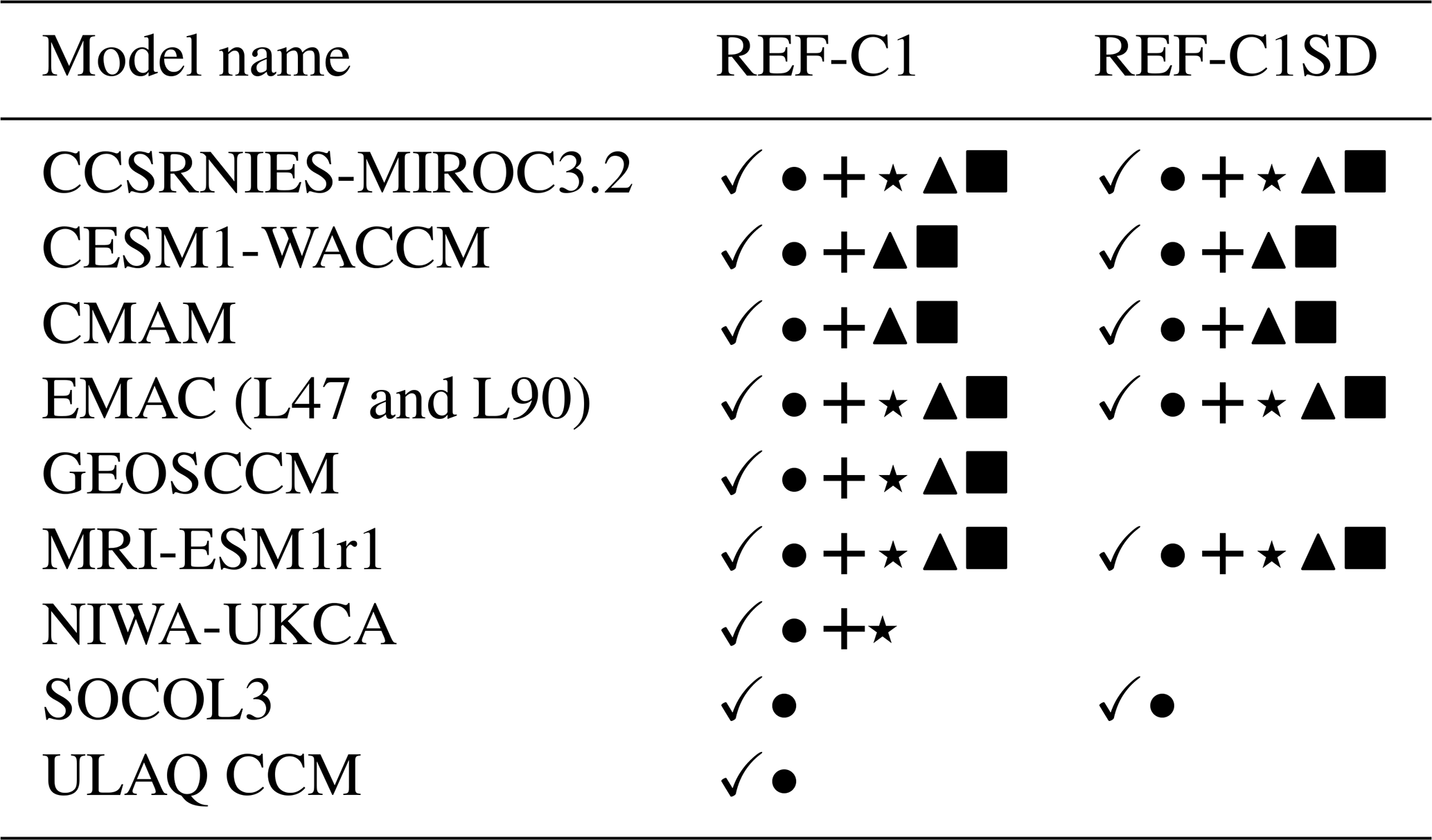
CCMI is the successor activity to CCMVal-2 and the Atmospheric Chemistry and Climate Model Intercomparison Project (ACCMIP; Lamarque et al., 2013). We use the hindcast free-running simulations, REF-C1, and the nudged specified dynamics simulations, REF-C1SD, which cover the periods 1960–2009 and 1980–2009, respectively. Here we analyse the common 30-year period 1980–2009 that was run by all models for both experiments with prescribed observed SSTs and sea ice concentrations. The CCMI data were downloaded from the British Atmospheric Data Centre (Hegglin and Lamarque, 2015). For an extensive overview of the CCMI models, see Morgenstern et al. (2017). We analyse those CCMI models that output the necessary TEM diagnostics. At a minimum, this requires the residual vertical velocity () and the residual meridional velocity (; Andrews et al., 1987); where available we also use the resolved and parameterized wave forcing fields from the models. This gives results from a total of 10 models, which differ from one another in various aspects, such as their horizontal resolution, ranging from 1.9 to 5.6∘, their vertical resolution, and their sub-grid parameterizations (see Table 1). The main text concentrates on the 7 out of 10 models that performed both the REF-C1 and REF-C1SD experiments (Table 2). However, the broad conclusions drawn in the main text for the characteristics of the seven-member REF-C1 ensemble are consistent with the behaviour for all 10 models. Hence the three models that only performed the REF-C1 experiment (GEOSCCM, NIWA-UKCA, and ULAQ-CCM) are not discussed further, but for completeness a subset of diagnostics from those models is shown in the Supplement (Figs. S1–S5).
Table 1CCMI models that provided TEM diagnostic model output used in this study. CP is Charney–Phillips, T21 ≈ 5.6∘ × 5.6∘, T42 ≈ 2.8∘ × 2.8∘, T47 ≈ 2.5∘ × 2.5∘, TL159 ≈ 1.125∘ × 1.125∘, TA is hybrid terrain-following altitude, TP is hybrid terrain-following pressure, and NTP is non-terrain-following pressure.

For the REF-C1 simulations we analyse between one and five ensemble members (depending on what was available), and for REF-C1SD the one realization submitted from each model. The REF-C1SD simulations nudge temperature and other meteorological fields such as horizontal winds, vorticity and divergence, and some surface fields (Table 2), while the chemical fields are left to evolve freely. The nudging timescales range from 6 to 50 h, and the height range over which nudging is applied varies (Table 2). The TEM and related diagnostics that were available from each model are shown in Table 3. The models use different reanalysis fields for nudging taken from ERA-Interim (Dee et al., 2011), JRA-55 (Ebita et al., 2011; Kobayashi et al., 2015), or MERRA (Rienecker et al., 2011). The differences in the residual circulation diagnosed from reanalyses have been identified and documented in previous studies (e.g. Abalos et al., 2015).
Table 2Details of nudging in the CCMI REF-C1SD simulations that provided TEM diagnostics model output used in this study. ERA-I is ERA-Interim, CIRA is Cooperative Institute for Research in the Atmosphere, MERRA is Modern-Era Retrospective reanalysis, and JRA-55 is Japanese 55-year Reanalysis. T (with wave 0) for EMAC refers to the additional nudging of the global mean temperature.

Table 3Available TEM-related model output for each model from the CCMI-1 archive: (✓), (•), EPFD (+), gravity wave drag (OGWD and NOGWD; ⋆), OGWD (▴), and NOGWD (▪).
2.2 Model diagnostics
2.2.1 TEM residual circulation
The TEM velocities () are defined as (Andrews et al., 1987)
where is the residual meridional mass streamfunction, ρ0 is log-pressure density, α is Earth's radius, and ϕ is latitude. As most of the models analysed here use a hybrid-pressure vertical coordinate, the prognostic variable is the pressure vertical velocity (calculated in Pa s−1), which must be converted to metres per second in order to get the residual vertical velocity, . The conversion of ω to w in isobaric coordinates is given by the following equation:
where p is pressure, R=287 J K−1 kg−1 is the gas constant for dry air, and H is a fixed scale height. Both TEM velocity components were submitted as monthly mean fields to the CCMI data archive. Upon close examination of the CCMI model output, some discrepancies were found in the way that the residual vertical velocity was calculated among the models. Although a fixed scale height of H=6950 m was recommended in the CCMI data request (Eyring et al., 2013; Hegglin and Lamarque, 2015), the TEM output from some models (EMAC and SOCOL3) was calculated incorrectly using a temperature-dependent density, , instead of the log-pressure definition of the density, , such that z has a unique 1:1 correspondence with p. This methodological error leads to artificial spread in the model fields. We note that previous multi-model comparisons of the residual circulation that use taken directly from models may have been subject to the same issue (e.g. Butchart et al., 2010; SPARC, 2010), though we cannot confirm this. To avoid this methodological inconsistency, Dietmüller et al. (2018) recalculated from using the continuity equation, which requires a vertical integration and a derivative along the meridional direction. The recalculation of from was also explored for this study, but it was found to introduce additional errors affecting the latitudinal structure of (not shown) specifically because of the reduced number of CCMI-requested pressure levels compared to the native model levels. We were able to overcome the discrepancy in the submitted fields for the EMAC simulations by reconverting high-frequency output to using the log-pressure density as in Eq. (2). However, for SOCOL3 the required output for this was not available, and hence we use the submitted for which the absolute values should be treated with caution. For the other models, the results presented in this study are based on the original diagnostics submitted to the CCMI data archive, which we have verified were calculated in the correct way.
We compute the mass flux across a given pressure surface as (Rosenlof, 1995)
using the boundary condition in which Ψ=0 is at the poles. By finding, at each pressure level, the latitude at which Ψmax and Ψmin occur, which corresponds to the height-dependent turnaround (TA) latitudes, we can calculate the net downward mass flux in each hemisphere. The net tropical upward mass flux, equal to the sum of the downward mass fluxes in each hemisphere, can then be expressed as (Rosenlof, 1995)
The tropical upward mass flux (TUMF) has been used widely as a measure of the strength of the BDC (e.g. Rosenlof, 1995; Butchart and Scaife, 2001; Butchart et al., 2006, 2010, 2011; Butchart, 2014, and references therein; Seviour et al., 2012), so its use here enables a direct comparison with earlier studies. Arguably, the strength of the TUMF is a first-order metric for evaluating changes in the stratospheric mass circulation as a consequence of nudging. As mentioned above, by calculating the annual means of TUMF accounting for the seasonal cycle of the TA latitudes, we capture the correct evolution of the intra-seasonal (not shown) and inter-annual variability in the TUMF.
2.2.2 Downward control principle calculations
Under steady-state conditions, at a specified latitude φ and log-pressure height z is given by the vertically integrated eddy-induced total zonal force, , above that level (Haynes et al., 1991):
where in the quasi-geostrophic limit, . The above integration applies along lines of constant mean absolute angular momentum per unit mass, , where is the zonal mean zonal wind and Ω is Earth's rotation rate, with boundary conditions of Ψ→0 and as z→∞. These lines of constant angular momentum are approximately vertical except near the Equator (up to ∘) such that we can calculate the solution of the above integral using the constant φ for the limits of the integral (Haynes et al., 1991). In climate models, has contributions from resolved waves due to the Eliassen–Palm flux divergence (EPFD) and from parameterized gravity wave drag due to sub-grid-scale waves that originate from orography, convection and frontal instabilities. This enables us to estimate the contribution to the tropical upward mass flux of both resolved planetary wave driving (EPFD) and the orographic and non-orographic parameterized gravity wave drag (OGWD and NOGWD, respectively) from the CCMI model output (Table 3) and compare with the direct estimates derived from .
Applying the downward control principle (Haynes et al., 1991) can provide useful insights into the driving mechanisms of the stratospheric residual circulation and therefore explain part of the inter-model spread found in both REF-C1 and REF-C1SD simulations. While the downward control principle enables the contributions of EPFD and OGWD and NOGWD to TUMF to be calculated under various assumptions (Haynes et al., 1991), one has to keep in mind that the different wave forcings can interact and thus are not independent of each other (Cohen et al., 2013).
It is important to note some possible limitations of the diagnostic approaches chosen for this study. Both the direct and downward control principle methods rely on the applicability of quasi-geostrophic theory to interpret the results. In addition to the two approaches used here, the residual circulation can also be estimated using the thermodynamic equation. Studies have shown that the estimates from the different methods for evaluating the residual circulation can differ (Seviour et al., 2012; Abalos et al., 2015; Linz et al., 2019), particularly in reanalyses where standard global conservation laws (e.g. conservation of mass) must generally not be met. Similar issues are likely to beset the nudged model simulations, owing to the additional tendencies included in the model equations. The differences between the calculation methods for the residual circulation can be as large as, or larger than, the differences between reanalysis datasets for the same diagnostic (Abalos et al., 2015; Linz et al., 2019) and may further depend on choices around averaging between fixed latitudes or the TA latitudes (Linz et al., 2019), so it is important to bear this in mind in interpretation of the results presented here. Unfortunately, heating rates were not available from all CCMI model simulations to perform the thermodynamic equation calculation. Nevertheless, we compute the direct and downward control principle diagnostics for the residual circulation in a self-consistent manner in the models and reanalyses to enable comparison with earlier multi-model studies (Butchart et al., 2006, 2010; SPARC, 2010).
2.3 Multiple linear regression model
To investigate the drivers of inter-annual variability in the residual circulation we apply a multiple linear regression (MLR) model (Eq. 6) to the annual mean time series of TUMF. The model includes terms for known drivers of variations in tropical lower-stratospheric upwelling: major volcanic eruptions (Pitari and Rizi, 1993), the El Niño–Southern Oscillation (ENSO; García-Herrera et al., 2006; Marsh and Garcia, 2007; Randel et al., 2009), the quasi-biennial oscillation (QBO; Baldwin et al., 2001), and a linear trend (Calvo et al., 2010):
where β0 is a constant, βi is the regression coefficient for basis function xi, and ε(t) is the residual. Following Maycock et al. (2018), the volcanic basis function is defined as the tropical lower-stratospheric average volcanic surface-area density (SAD), the ENSO basis function is the time series of eastern–central equatorial Pacific Ocean SST anomalies (Niño 3.4 index; 5∘ S to 5∘ N; 170 to 120∘ W); the two QBO terms are the first two principal-component time series from an empirical orthogonal function (EOF) analysis of the zonal mean zonal winds between 10∘ S and 10∘ N and 70 to 5 hPa and a linear trend. The first three regressors, the volcanic, ENSO, and the linear trend, are identical for both REF-C1 and REF-C1SD runs, while the QBO terms are calculated using the model winds for each model and experiment. For the REF-C1 runs, CMAM does not include a QBO; hence when we apply the MLR to the CMAM REF-C1 simulation the QBO terms are omitted. We opted not to include an equivalent effective stratospheric chlorine (EESC) MLR term to account for changes in ozone-depleting substances (Abalos et al., 2019; Morgenstern et al., 2018; Polvani et al., 2018, 2019), as the period considered in the study may not be sufficiently long for the linear trend to be separated properly from EESC. Since we are regressing annual mean TUMF we do not consider a seasonal cycle term or any lag in the terms. The results in Sect. 3.5 focus on the first ensemble member (in the rip-nomenclature, where r stands for realization, i for initialization, and p for physics – r1i1p1), but where applicable the results from the MLR model for the rest of the ensemble members of the REF-C1 runs are presented in the Supplement (Figs. S6–S9).
2.4 Reanalysis data
In order to compare the REF-C1 and REF-C1SD simulations against the reanalysis datasets used for the nudging, we use the SPARC Reanalysis Intercomparison Project (S-RIP) dataset (Martineau, 2017; Martineau et al., 2018). This provides a common gridded version of the reanalysis TEM fields on a 2.5∘ × 2.5∘ grid up to 1 hPa. The pressure vertical velocity, , is converted to the residual vertical velocity, , using Eq. (2). A detailed comparison of the stratospheric residual circulation in reanalysis datasets is given by Abalos et al. (2015).
3.1 Climatological residual circulation:
Figure 1 shows latitude–pressure cross-sections of the climatological (1980–2009) multi-model mean (MMM) annual mean for the REF-C1 (Fig. 1a) and REF-C1SD (Fig. 1b) simulations and their differences (Fig. 1c). In Fig. 1c absolute differences are computed, so positive values indicate where the magnitude of the circulation in REF-C1SD (whether upwelling or downwelling) is larger than in REF-C1. As expected, the climatologies show upwelling in the tropics between around 30∘ S to 30∘ N and downwelling at higher latitudes. In the lowermost stratosphere (100–80 hPa), within the region of tropical upwelling, the REF-C1SD MMM generally shows larger values in the subtropics and smaller values at the Equator compared to REF-C1, indicating a tendency for a more double-peaked structure in the tropics in the lowermost stratosphere (Ming et al., 2016a). Above this, between ∼ 70 and 4 hPa, the REF-C1SD MMM shows on average stronger upwelling at the Equator compared to REF-C1, indicating a less pronounced double-peaked structure in the REF-C1SD experiments in the lower stratosphere to middle stratosphere. Between 1 and 2 hPa, the REF-C1SD MMM shows larger inter-hemispheric asymmetry than in REF-C1, with stronger upwelling in the northern tropics (Fig. 1b). At the southern mid-latitudes, between ∼ 30 and 60∘ S, the REF-C1SD MMM exhibits on average slightly weaker downwelling than in REF-C1, with the largest magnitude differences found in the upper stratosphere. In the Arctic, the REF-C1SD MMM shows significantly stronger downwelling over the poles than in REF-C1. In the Antarctic the picture is more complex, with the REF-C1SD MMM showing weaker downwelling right at the pole in the upper stratosphere (2–10 hPa) but stronger downwelling between around 75 and 88∘ S. In the middle stratosphere, from 50 to 10 hPa, the REF-C1SD MMM shows stronger downwelling between 60 and 80∘ S.
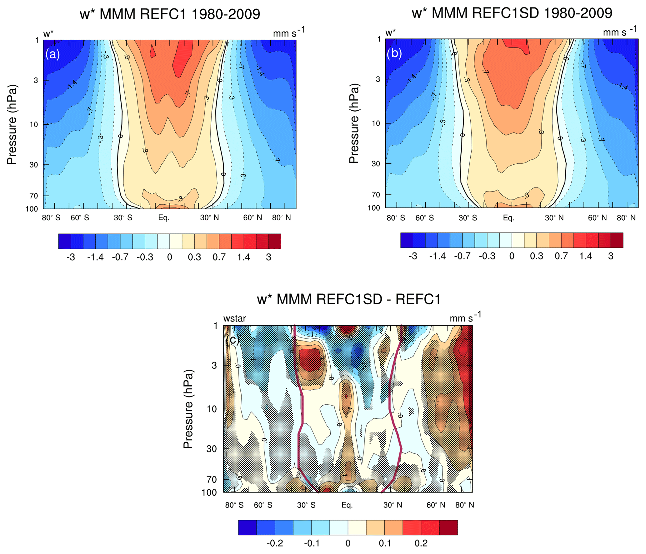
Figure 1Latitude vs. pressure climatology (1980–2009) of MMM annual mean for (a) REF-C1 simulations, (b) REF-C1SD simulations, and (c) the REF-C1SD–REF-C1 absolute differences. Shading denotes statistical significance at the 95 % confidence level, and the red lines in (c) denote the climatological turnaround latitudes in REF-C1SD.
To show the differences in the transition between regions of upwelling and downwelling motion, Fig. 2 shows vertical profiles of the climatological annual mean turnaround (TA) latitudes in each hemisphere for the REF-C1 and REF-C1SD MMM and the three reanalysis datasets used for nudging. Note that since five of the REF-C1SD models were nudged towards ERA-I, the REF-C1SD MMM may be more weighted towards ERA-I than the other reanalyses. In the NH, the REF-C1SD MMM shows a more poleward TA latitude compared to both REF-C1 and the reanalyses throughout almost the entire depth of the stratosphere (Fig. 2b). A more poleward TA latitude for REF-C1SD than in both REF-C1 and the reanalyses is also found in the Southern Hemisphere (SH) at pressures greater than 30 hPa (Fig. 2a). Hence the nudged simulations show, on average, a wider region of tropical upwelling in the lower stratosphere compared to their free-running counterparts by up to around 5∘ latitude. In the middle stratosphere and upper stratosphere the REF-C1SD MMM shows a narrower upwelling region in the SH. Interestingly, above 10 hPa in the SH (Fig. 2a), the REF-C1SD does not show a progressive widening of the upwelling region with decreasing pressure as seen in the reanalyses. This is reflected in the structural differences in in the SH upper stratosphere found in some models (Fig. S10). It should be noted though that the differences in TA latitudes between the REF-C1 and REF-C1SD MMMs are comparable to the differences found between the three reanalysis datasets.
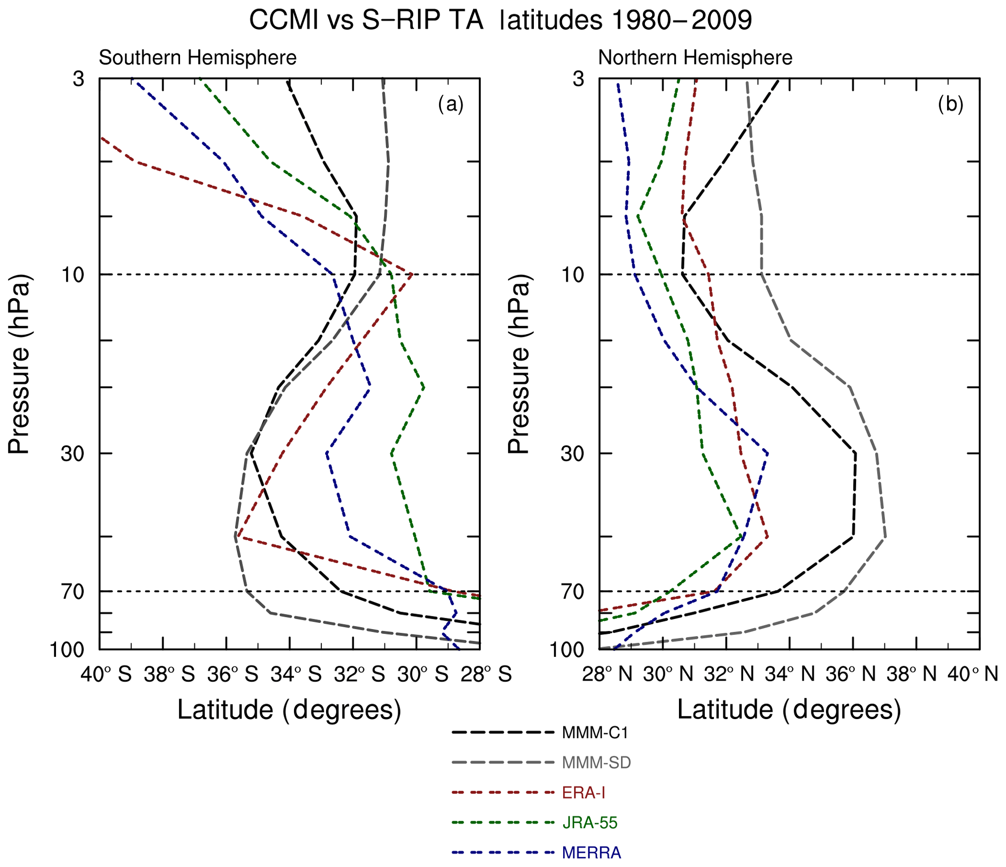
Figure 2Vertical profiles of the climatological turnaround latitudes in the stratosphere for the MMM of the REF-C1 runs (black dashes), the MMM of the REF-C1SD runs (grey dashes), and the S-RIP reanalysis datasets (ERA-I, JRA-55, and MERRA) for the (a) Southern Hemisphere and (b) Northern Hemisphere.
Focusing on the lower stratosphere, Fig. 3 shows the climatological annual mean at 70 hPa in the individual models for the (a) REF-C1 and (b) REF-C1SD simulations and (c) their differences. Also plotted in Fig. 3b is from the reanalyses, and Fig. 3d shows the difference between each REF-C1SD simulation and the reanalysis they were nudged towards. Within the upwelling region, all the models show a clear double-peaked structure in the tropics, with the exception of the CCSRNIES-MIROC3.2 and MRI-ESM1r1 models in the REF-C1SD experiment. In those two cases, CCSRNIES-MIROC3.2 simulates a tri-modal structure, while MRI-ESMr1 shows a relatively constant across the tropics. For the REF-C1 experiment, both EMAC simulations, CMAM and SOCOL3, show a narrower double-peaked structure, with EMAC-L47 exhibiting a rather pronounced NH subtropical maximum. Conversely, CESM1-WACCM simulates the broadest region of tropical upwelling in the lower stratosphere, with the SH subtropical maximum occurring at higher latitudes compared with the rest of the models. The other REF-C1 simulations also exhibit a double-peaked structure, which is generally more hemispherically symmetric, but with varying amplitudes.
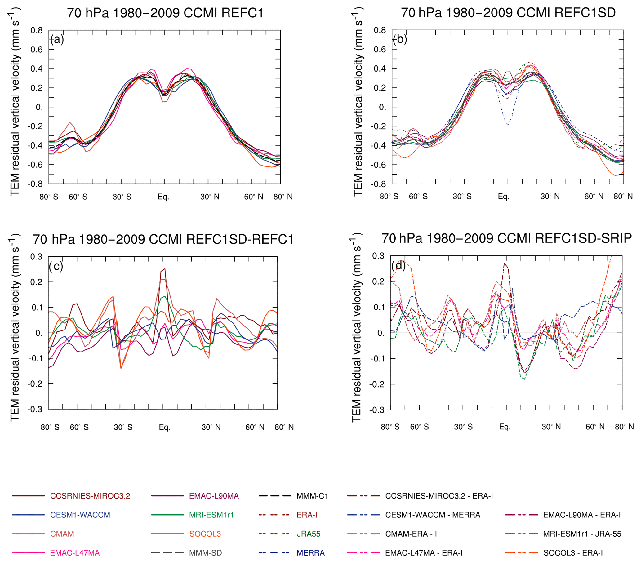
Figure 3Mean strength of annual mean (mm s−1) at 70 hPa for (a) REF-C1 free-running models, (b) REF-C1SD nudged models, (c) absolute differences between the REF-C1SD and REF-C1 experiment for each model, and (d) absolute differences between each REF-C1SD simulation and the respective reanalysis used for nudging.
A double-peaked structure in the lower stratosphere has previously been shown in reanalysis datasets (Abalos et al., 2015; Ming et al., 2016a) and some CCMs (Butchart et al., 2006, 2010). This can also be seen in Fig. 3b for the three reanalysis datasets (ERA-I, JRA-55, and MERRA), where ERA-I and JRA-55 show an asymmetric double-peaked structure with stronger upwelling in the NH subtropics compared to the SH. As documented by Abalos et al. (2015), based on the direct calculation of the residual circulation, MERRA exhibits downwelling at the Equator, an issue which was highlighted in Abalos et al. (2015) and manifested as a negative cell in the streamfunction.
Figure 3c shows the absolute differences in at 70 hPa between the REF-C1SD and REF-C1 experiments. Positive values show where the magnitude of the circulation in REF-C1SD is larger than in REF-C1. The largest differences are generally found within the inner tropics, where CCSRNIES-MIROC3.2, CMAM, and MRI-ESM1r1 exhibit significantly stronger upwelling (up to 3 times more for CMAM) near the local minimum at the Equator. There are also larger differences in many models near edges of the upwelling region (30–40∘ S), which reflect differences in the width of the tropical pipe between the free-running and nudged simulations (Fig. 2 and Sect. 3.3). Around the subpolar and polar latitudes of the SH, the majority of the REF-C1 models simulate stronger downwelling than their nudged counterparts, while in the NH extratropics no consistent picture emerges across the models. EMAC-L47 and EMAC-L90 show markedly different behaviours despite the fact they are nudged towards the same reanalysis (ERA-I) and differ only in their vertical resolution. This indicates that the effect of nudging on the mean residual circulation is likely to be sensitive to a great number of factors that vary from model to model.
Another interesting result from Fig. 3 is that the inter-model spread in for both experiments is larger in the NH downwelling region than in the equivalent region of the SH. Specifically, the inter-model spread is 0.14 mm s−1 for the REF-C1 runs for all points between 30 and 80∘ S and 0.2 mm s−1 for points between 30 and 80∘ N, while for REF-C1SD the values are 0.12 and 0.19 mm s−1, respectively. This also demonstrates that the inter-model spread in in the REF-C1SD simulations is comparable to that in REF-C1 at extratropical latitudes. In contrast, in the tropics between 30∘ S and 30∘ N the REF-C1SD simulations exhibit a slightly larger inter-model spread than the free-running simulations (0.09 mm s−1 vs. 0.07 mm s−1).
Figure 3d shows the absolute differences in between the REF-C1SD simulations and the respective reanalysis dataset used for nudging. In the upwelling region, the REF-C1SD experiments generally show stronger upwelling near the Equator than in the reanalyses. Although CESM1-WACCM is nudged towards MERRA, it does not simulate downwelling at the Equator as seen in the MERRA direct estimate. The relatively larger differences near 10–15∘ N in CCSRNIES-MIROC3.2, EMAC-L90, and MRI-ESMr1 reflect a lack of inter-hemispheric asymmetry in the double-peaked structure in the REF-C1SD experiment compared to the reanalyses. Outside of the tropics, the REF-C1SD experiments generally show weaker downwelling in the NH mid-latitudes, while at polar latitudes (>65∘) the REF-C1SD runs consistently show stronger downwelling than in the reanalyses. The difference in at high latitudes between the REF-C1SD and reanalysis datasets extends throughout the depth of the stratosphere (see Fig. S10). More generally, Fig. 3b shows that the different models that all nudge towards ERA-I (CCSRNIES-MIROC3.2, CMAM, EMAC-L47 and EMAC-L90, and SOCOL3) produce very different mean residual circulations.
In summary, we conclude based on the results in Figs. 1 to 3 that nudging meteorology affects the strength and structure of the climatological residual circulation throughout the stratosphere. However, as implemented in these simulations (Table 2), nudging neither strongly constrains the mean amplitude and structure of the residual circulation nor produces circulations that closely resemble the direct estimates from the reanalyses.
3.2 Climatological residual circulation: tropical upward mass flux
Figure 4 shows vertical profiles of the climatological TUMF between 100 and 3 hPa calculated from annual means of for the (a) REF-C1 and (b) REF-C1SD experiments and (c) their difference. Note the logarithmic x-axis scale and that the CCMI and S-RIP fields have been interpolated from their native model levels to a set of predefined common pressure levels, which are rather sparse in the upper stratosphere; hence the TUMF calculation could be different if it were performed on the native model grid of both CCMI models and the reanalyses.
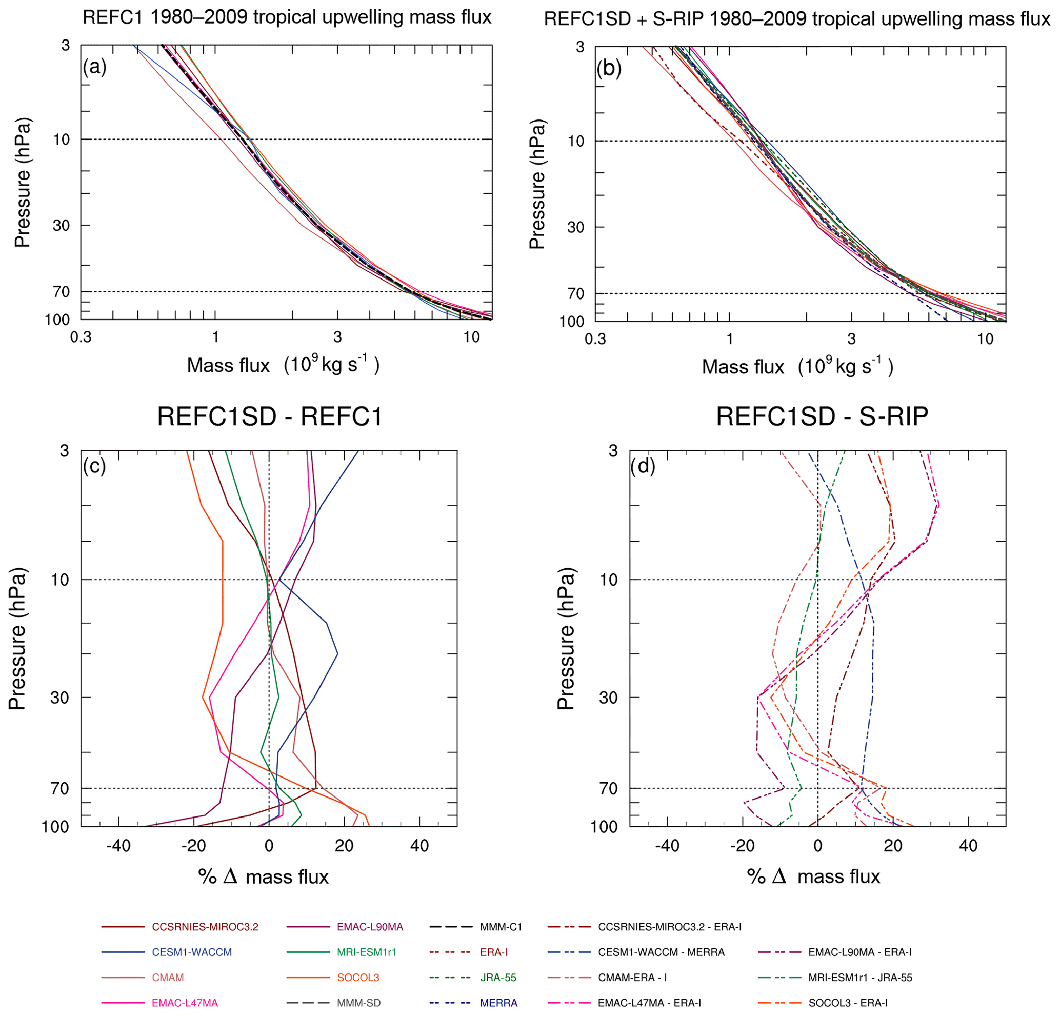
Figure 4Vertical profiles of climatological (1980–2009) tropical upward mass flux (109 kg s−1) averaged between the turnaround latitudes for (a) REF-C1 and (b) REF-C1SD, (c) differences (%) between REF-C1SD and REF-C1, and (d) % differences between REF-C1SD and the respective reanalysis used for nudging. Note the logarithmic x axis in panels (a) and (b).
In terms of the differences between the REF-C1SD and REF-C1 simulations (Fig. 4c), there is no consistent picture of the effect of nudging on the TUMF at different stratospheric levels. In the lowermost stratosphere between 70 and 100 hPa, most models (apart from EMAC-L90) simulate stronger TUMF in the REF-C1SD runs than in REF-C1. The largest TUMF differences in the lower stratosphere due to nudging occur in EMAC-L90 and SOCOL3, which show differences at 90 hPa of around −20 % and +25 %, respectively. In the middle stratosphere, between 10 and 70 hPa, some models show almost no difference in TUMF due to nudging (MRI-ESMr1), some show a stronger mass flux (CCSRNIES-MIROC3.2, CESM1-WACCM, and CMAM) and others show a weaker mass flux (EMAC-L47 and SOCOL3). In the upper stratosphere (above 10 hPa) the picture is also mixed, as half of the models show higher TUMF in the nudged experiments (CESM1-WACCM and EMAC-L47 and EMAC-L90) and the others show weaker TUMF (CCSRNIES-MIROC3.2, MRI-ESM1r1, and SOCOL3). CMAM shows the smallest change in TUMF in the upper stratosphere due to nudging. CESM1-WACCM is the only model to show a consistent sign of the TUMF differences between REF-C1SD and REF-C1 at all levels, with higher TUMF found throughout the stratosphere. There is no apparently simple relationship between the free-running model TUMF climatologies (Fig. 4a) and the effect of nudging (Fig. 4c).
We now compare the TUMF in each REF-C1SD experiment with the reanalysis it was nudged towards (Fig. 4d). Taking at first a broad view of the entire profiles, there is a resemblance between the profiles of TUMF differences in EMAC-L47 and SOCOL3 as compared to ERA-I, which may be related to the similarities in the implementation of nudging in these models; for example, vorticity and divergence were nudged with the same relaxation parameters (see Table 2). The CESM1-WACCM REF-C1SD simulation generally shows larger TUMF values than MERRA by up to 10 %–15 % apart from in the upper stratosphere, where they start to converge. MRI-ESM1r1 exhibits relatively better agreement of TUMF with JRA-55 throughout the stratosphere. Looking across the models, most of the REF-C1SD simulations simulate stronger upwelling than their respective reanalysis in the upper stratosphere, with differences reaching up to 30 %–35 % in the two EMAC models. In fact, EMAC-L47 and EMAC-L90 show a high degree of similarity in the vertical structure of the TUMF differences between REF-C1SD and ERA-I at pressures less than 30 hPa, despite showing substantial differences in the lower stratosphere. This could be because in EMAC nudging is only imposed strongly up to 10 hPa, while higher model layers have weakening nudging coefficients, as they serve as transition layers. In the middle stratosphere (50–20 hPa), most of the REF-C1SD models simulate a lower TUMF compared to the reanalysis. Again, a key message is that the nudged REF-C1SD simulations show a comparable, if not a slightly larger, spread in the climatological TUMF compared to the free-running REF-C1 simulations throughout almost the whole depth of the stratosphere.
To understand the dynamical factors that contribute to the modelled climatological residual circulation and its spread, Fig. 5 shows the annual mean TUMF at 70 hPa along with the downward control calculations (Sect. 2.2.2) to quantify the contribution of resolved and parameterized wave forcing to the TUMF. The black bars on the left show the TUMF diagnosed from , and the grey bars on the right show the estimated contribution to TUMF from the EPFD (dark grey) and the orographic (medium grey) and non-orographic (light grey) gravity wave drag. Note that SOCOL3 did not provide wave forcing fields (Table 3), so we cannot perform the downward control calculations for that model.
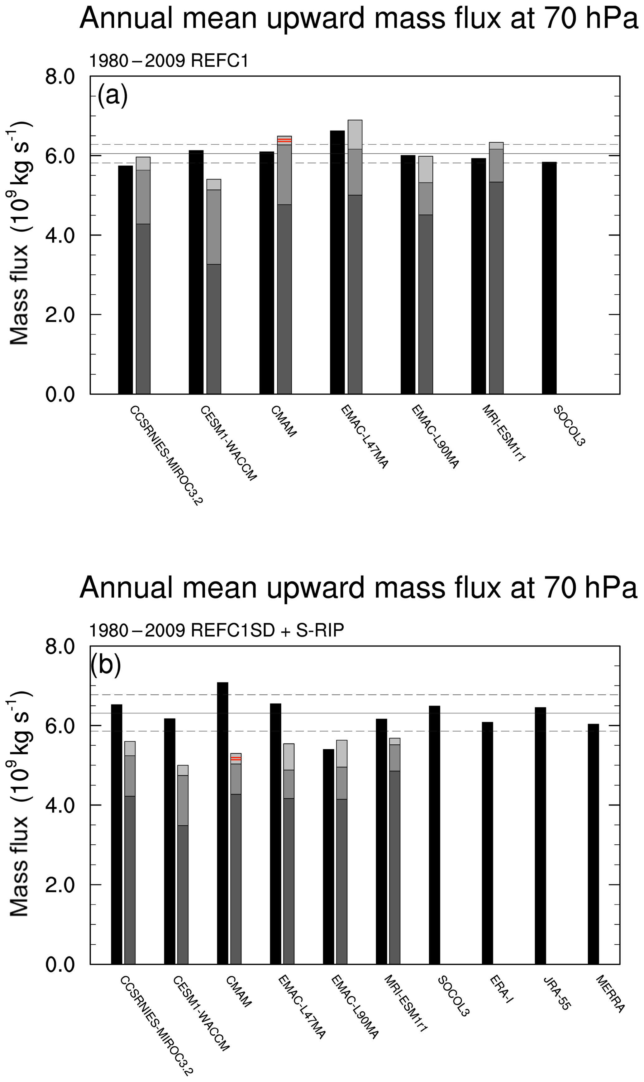
Figure 5Tropical upward mass flux at 70 hPa (left bars) along with downward control calculations (right bars) showing contributions from EPFD (dark grey), OGWD (medium grey), and NOGWD (light grey) for (a) REF-C1 and (b) REF-C1SD and the reanalyses. For CMAM, the NOGWD contributes negatively to TUMF and is indicated with two red horizontal lines inside the lighter grey bar.
In the free-running REF-C1 simulations (Fig. 5a), the estimated TUMF from the total wave forcing for the majority of the models (apart from CESM1-WACCM and EMAC-L90) slightly exceeds the TUMF calculated directly from . Since these simulations are internally consistent, the imperfect match indicates that the downward control principle as applied here relies on the close but inexact applicability of certain assumptions, such as the system being in a steady state in response to a steady mechanical forcing (Haynes et al., 1991). The REF-C1 inter-model range in TUMF at 70 hPa is 5.74×10⁹ to 6.62×10⁹ kg s−1 (inter-model standard deviation of 0.29×10⁹ kg s−1). Comparing the CCMI results in Fig. 5a with the results from CCMVal-2 models (see Fig. 4.10; SPARC, 2010), the MMM TUMF at 70 hPa for the seven REF-C1 model simulations analysed here (6.05×10⁹ kg s−1) is within the inter-model range of the 14 CCMVal-2 models, which show a MMM TUMF around 4 % weaker (5.8×10⁹ kg s−1; SPARC, 2010). In terms of the contribution of the resolved wave forcing to the TUMF in the free-running simulations, there appears to be a decreased inter-model range (3.26×10⁹ to 5.33×10⁹ kg s−1) in the present study compared with the CCMVal-2 models, albeit that study included more models (1.5×10⁹ to 5.5×10⁹ kg s−1; SPARC, 2010). Some CCMI models have increased their horizontal resolution by up to a factor of 2 (CMAM, MRI-ESM1r1, SOCOL3) and also their vertical resolution by up to 80 vertical levels (MRI-ESM1r1) compared with CCMVal-2 models (Dietmüller et al., 2018), which could improve their ability to simulate resolved wave forcing. There is a notable feature of CMAM which shows that the NOGWD contributes negatively to TUMF (indicated with two red horizontal lines on Figs. 5 and S11); this was also found for CMAM in CCMVal-2 (Fig. 4.10; SPARC, 2010).
The MMM TUMF at 70 hPa in the REF-C1SD simulations (Fig. 5b) is 6.32×10⁹ kg s−1, or around 5 % higher than in REF-C1. The REF-C1SD model range is larger than in REF-C1, being 5.39×10⁹ to 7.08×10⁹ kg s−1 (inter-model standard deviation of 0.51×10⁹ kg s−1). A notable feature is that the contribution from the individual and total wave forcing contributions shows reduced inter-model spread in the REF-C1SD simulations (Fig. 5b; darker grey bars). For example, the inter-model standard deviation of the EPFD contribution to TUMF at 70 hPa is around 40 % smaller than in REF-C1 (0.44×10⁹ and 0.72×10⁹ kg s−1, respectively). Nonetheless, the residuals (i.e. the difference between the directly calculated TUMF and the total downward control estimated contribution from the wave forcing) are substantially larger and more positive (except for EMAC-L90) in the REF-C1SD experiment than in REF-C1. This shows that nudging adds an additional non-physical tendency in the model equations which acts to decouple the wave forcing from the residual circulation; this means that the physical constraint that the divergence of the angular momentum flux due to the mean motion is balanced over some sufficient time average by that of all eddy motions does not apply in the nudged models (Haynes et al., 1991). The details of how this decoupling is manifested are likely to vary from one model to another, depending on multiple factors such as nudging timescales, nudging parameters, nudging height range, and model resolution. Comparison of the TUMF at 10 hPa for the REF-C1SD experiment (see Fig. S11b) also reveals substantial differences in some models between the direct and downward control TUMF estimates in the middle stratosphere. Variations in the residuals as a function of height may indicate differences in the effect of nudging on the connection between the climatological wave forcing and the shallow and deep branches of the circulation (Birner and Bönisch, 2011). However, the inter-model ranges in the directly calculated TUMF at 10 hPa are more comparable in the two experiments than those found at 70 hPa (1.45×10⁹ to 1.70×10⁹ and 1.51×10⁹ to 1.72×10⁹ kg s−1 for REF-C1 and REF-C1SD, respectively; Fig. S11b).
Interestingly, for the single simulations that were nudged towards MERRA and JRA-55 (CESM1-WACCM and MRI-ESM1r1, respectively), the TUMF at 70 hPa in the REF-C1SD runs appears to be close to the estimates from the reanalyses they are nudged towards (compare black bars in Fig. 5b). This may simply be a coincidence given that there are substantial differences in the structure of between the REF-C1SD simulations for those models and the reanalyses (Fig. 3b and d), and this is not found for all five models that were nudged towards ERA-I. Indeed, given that there is substantial spread in TUMF amongst the five REF-C1SD models nudged to ERA-I, it is likely that the differences between the REF-C1SD and reanalysis datasets are related to how nudging was implemented in each model; a wide variety of relaxation timescales and vertical nudging ranges were used by the models (Table 2). Despite this, the lower TUMF calculated directly from in EMAC-L90 compared to EMAC-L47, seen in both the REF-C1 and REF-C1SD experiments, is consistent with the results of Revell et al. (2015b), who also find that an increase in the model vertical resolution for SOCOL3 results in a slowdown of the BDC.
In summary, the results from Figs. 4 and 5 further demonstrate that nudging imparts an external and non-physical tendency in the model equations, which in turn might cause violations of the normal constraints on the global circulation, such as conservation of momentum and energy. This is found to alter the residual circulation but in a manner that cannot be understood from a closure of the circulation through the integrated wave forcing, as would ordinarily apply in the downward control principle (Haynes et al., 1991).
3.3 Annual cycle
We now evaluate the representation of the annual cycle in the residual circulation. Figure 6 shows the MMM climatological annual cycle of at 70 hPa for the REF-C1 and REF-C1SD simulations and their difference. Both experiments show similar broad features in the annual cycle, with stronger tropical upwelling in boreal winter, a latitudinal asymmetry in the region of upwelling, with the TA latitude being further poleward in the summer hemisphere, and stronger downwelling over the winter pole. These features resemble the annual cycle found in other multi-model studies (e.g. Hardiman et al., 2014). Figure 6c shows that on average the nudged models simulate stronger upwelling in the subtropics, particularly in the NH in boreal winter, with a few exceptions, the most prominent one being the narrow band between the Equator and 10∘ N, where the REF-C1 simulations exhibit stronger upwelling in austral winter. Consequently, the nudged models simulate substantially stronger downwelling in the mid-latitudes in winter. In the NH mid-latitudes in the summer months, nudged runs show weaker downwelling, which reverses for the SH mid-latitudes in the austral winter. At polar latitudes there is a distinct seasonality to the differences between the REF-C1SD and REF-C1 simulations, with the nudged models simulating stronger downwelling in boreal winter and weaker downwelling in the Arctic during the rest of the year, corresponding to an amplified annual cycle. Conversely in the Antarctic, the REF-C1SD simulations generally simulate weaker downwelling, particularly during austral summer and spring.
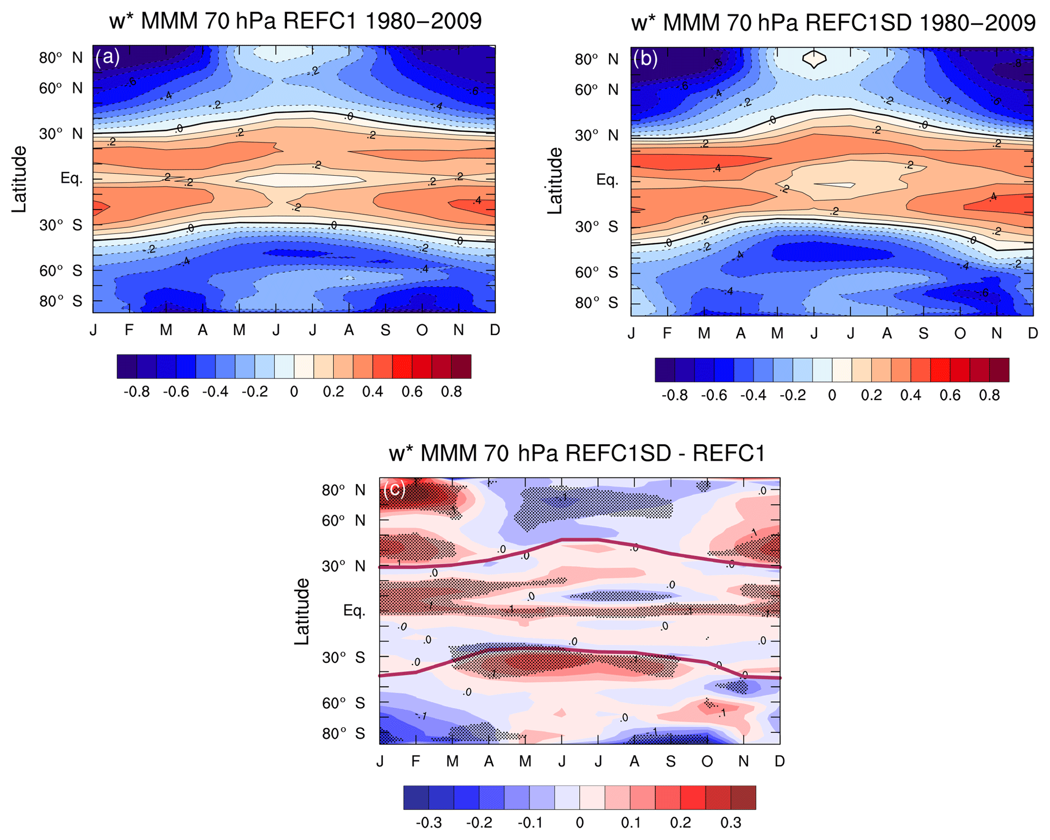
Figure 6Climatological MMM annual cycle in (mm s−1) at 70 hPa for (a) REF-C1, (b) REF-C1SD, and (c) the REF-C1SD minus REF-C1 absolute differences. The shading in (c) denotes regions where the differences are statistically significant above 95 % using a two-tailed Student's t test. The turnaround latitudes () are shown by the thick black lines in (a) and (b) and by the thick red lines for the REF-C1SD MMM in (c).
To compare the annual cycle in residual circulation in the individual models, Fig. 7a and b show the mean tropical (30∘ S–30∘ N) at 70 hPa for the REF-C1 and REF-C1SD simulations, respectively. Comparing the MMM annual cycle of the REF-C1 runs (Fig. 7a) with the MMM REF-C1SD (Fig. 7b) reveals that on average the nudged models show a slightly larger peak-to-peak annual cycle amplitude (0.16 mm s−1 vs. 0.13 mm s−1). In general, the amplitude of the annual cycle in tropical mean is slightly more constrained across the REF-C1SD simulations with the spread in peak-to-peak amplitude, as measured by the inter-model standard deviation, being around 25 % smaller than in REF-C1 (σ=0.015 mm s−1 vs. 0.020 mm s−1, respectively). In terms of seasonal mean behaviour, the nudging appears to constrain the tropical mean in boreal summer (June–July–August – JJA), which exhibits ∼20 % less spread than in the REF-C1 experiments, but it does not constrain the tropical mean in boreal winter (December–January–February – DJF), which shows a larger spread than the free-running models by a factor of 2. Furthermore, the differences in tropical mean between the REF-C1SD runs and the respective reanalysis they are nudged towards are generally larger in boreal winter than in boreal summer for most models. In terms of spatially resolved differences in between REF-C1SD and the reanalyses (Fig. S12), some consistent features include the REF-C1SD simulations showing stronger downwelling in the Arctic in boreal winter compared to the reanalyses and showing weaker upwelling in the northern subtropics in boreal summer and autumn. Overall, the REF-C1SD minus reanalysis differences for the individual models highlight a wide variety in both the magnitude and the spatial patterns of their absolute differences, with no consistent picture emerging even for the models nudged towards the same reanalysis dataset.

Figure 7(a, b) Climatological annual cycle in (mm s−1) at 70 hPa between 30∘ S and 30∘ N in (a) REF-C1 and (b) REF-C1SD. (c, d) Climatological annual cycle in turnaround latitudes at 70 hPa for each model in (c) REF-C1 and (d) REF-C1SD.
Figure 7c and d show the climatological annual cycle in the TA latitudes at 70 hPa for the REF-C1 and REF-C1SD runs, respectively. This further breaks down the MMM annual mean perspective shown in Fig. 2 by model and by season. In the SH, the spread in seasonal mean TA latitude across models, as measured by the intermodel standard deviation, is increased in the REF-C1SD experiment in all seasons by up to 30 % compared to REF-C1. Conversely in the NH, the spread in seasonal mean TA latitude is decreased for REF-C1SD in all seasons except boreal spring (MAM), where it is increased. There are also substantial differences between the TA latitudes in the REF-C1SD experiment and the reanalyses in all months, which shows that nudging does not produce consistent structures of regions of upwelling and downwelling to those in the reanalysis. To summarize the results of Fig. 7, there is substantial inter-model spread in the TA latitudes and in the amplitude of the annual cycle in , highlighting significant inter-hemispheric differences in the upwelling region between both sets of simulations and between the nudged experiment and the reanalyses.
3.4 Interannual variability in the tropical upward mass flux
Figure 8 shows time series over 1980–2009 for the annual, DJF, and JJA mean TUMF at 70 hPa for the REF-C1 (left column) and REF-C1SD (right column) simulations. As expected, the TUMF is larger in DJF compared to the annual and JJA means in both the REF-C1 and REF-C1SD runs because the average tropical upwelling is stronger in boreal winter. The individual REF-C1SD simulations show remarkably similar temporal variability in contrast to REF-C1, where the modelled inter-annual variability is very diverse despite the models all being forced with observed SSTs. Hence, although nudging does not constrain the mean TUMF in the lower stratosphere, it constrains the inter-annual variability; this is even more apparent for the DJF and JJA seasonal means (Fig. 8d, f). Additionally, the REF-C1SD simulations show a relatively high agreement in their temporal variability to the reanalysis datasets they were nudged towards, albeit with differences in magnitude and trend at the beginning of the 21st century, where ERA-I and MERRA show a decrease in TUMF.

Figure 8Top to bottom: time series of annual, DJF, and JJA means of tropical upward mass flux (×109 kg s−1) at 70 hPa for (a, c, e) REF-C1 and (b, d, f) REF-C1SD.
To investigate the cause of the high temporal coherence of the REF-C1SD TUMF time series, Fig. 9 presents the annual mean TUMF anomalies at 70 hPa along with the relative contributions from EPFD, OGWD, NOGWD, and the total parameterized wave forcing (from top to bottom panels) for REF-C1 (left column) and REF-C1SD (right column), respectively. Figure 9b shows again the remarkably similar temporal variability in TUMF across the REF-C1SD runs, which can be contrasted against the weak inter-annual coherence in the REF-C1 runs (Fig. 9a). Figure 9d and j show that both the EPFD and the total parameterized wave forcing contributions to the TUMF show a high degree of temporal coherence in the REF-C1SD simulations. The fact that the individual OGWD and NOGWD terms do not show such a strong inter-model agreement, while the total parameterized wave forcing does, could suggest that there is some compensation occurring between the different parameterized wave forcing components (e.g. Cohen et al., 2013). It should be noted that the reanalyses have been shown to exhibit strong similarities in their resolved EP fluxes as shown by the linear correlation in the time series of tropical upwelling at the 70 hPa level when considering the momentum balance estimates of (Abalos et al., 2015). This result indicates that although nudging does not constrain the mean residual circulation, it constrains the inter-annual variability and produces similar contributions to variability across models from both resolved and parameterized wave forcing. In contrast, the REF-C1 simulations show a highly variable pattern of the estimated TUMF anomalies from EPFD and parameterized wave forcing (Fig. 9c and i), despite the fact that they use the same observed SSTs and that some nudge the phase of the QBO (CCSRNIES-MIRCO3.2, CESM1-WACCM, EMAC-L47 and EMAC-L90, and SOCOL3). In summary, the remarkably coherent inter-annual variability in the annual TUMF time series in the REF-C1SD simulations is due to both the resolved and parameterized wave forcing being constrained by nudging; this is in strong contrast to the climatological strength of the TUMF, where there were large differences between the directly calculated TUMF and that due to wave forces (Fig. 5b). The reasons for the difference in the effect of nudging on the behaviour of the residual circulation between the long-term mean and inter-annual variability are unclear.
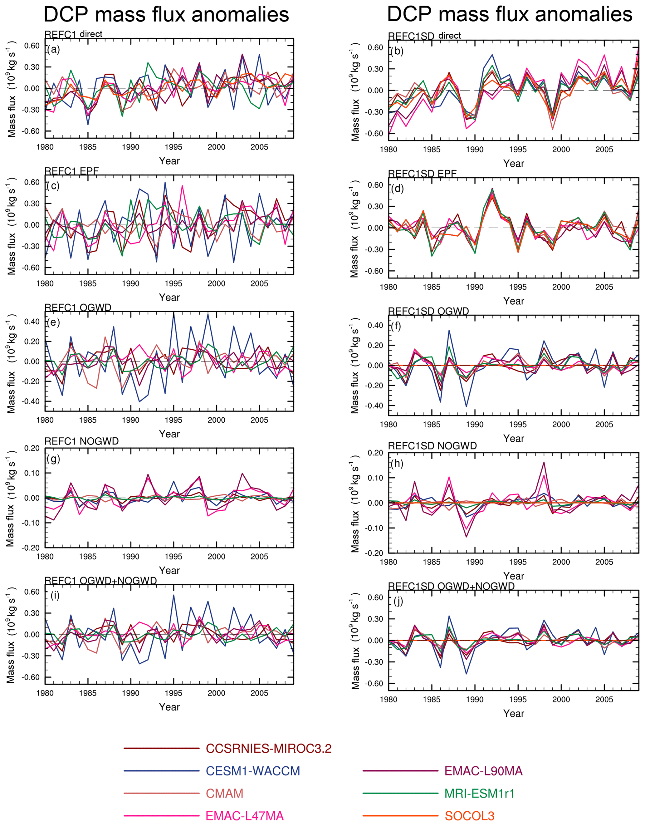
Figure 9Time series of the annual tropical upward mass flux anomalies (×109 kg s−1) calculated from (top to bottom) (a, b), and the downward control principle inferred contributions from resolved (EPFD) wave driving (c, d), orographic gravity wave drag (OGWD) (e, f), non-orographic gravity wave drag (NOGWD) (g, h), and from the total parameterized (OGWD and NOGWD) gravity wave drag (i, j) for REF-C1 (left panels) and REF-C1SD (right panels).
3.5 Multiple linear regression analysis
Figures 10 and 11 show time series of annual TUMF anomalies at 70 hPa attributed to each of the basis functions in the MLR model described in Sect. 2.3 and the regression residuals for the REF-C1 and REF-C1SD runs, respectively. Also shown in Figs. S13 and S14 are the regression coefficients for each term and for each model along with their uncertainties. Figure 10a shows a large spread in the diagnosed signal of volcanic eruptions in the TUMF time series. The majority of the REF-C1 simulations analysed here show a negative TUMF anomaly around the time of the El Chichón (1982) and Mount Pinatubo (1991) eruptions; however, the magnitude is within the estimated uncertainty range for all models except SOCOL3 (Fig. S13). In contrast to the REF-C1 results, most REF-C1SD simulations (except EMAC-L47 and EMAC-L90 – see above discussion) show a positive anomaly in TUMF attributed to volcanic eruptions (Fig. 11), consistent with earlier studies (Garcia et al., 2010; Diallo et al., 2017). However, there is still a considerable range of amplitudes, and only the CESM1-WACCM and MRI-ESM1r1 regression coefficients are highly significant (Fig. S14). The issue of establishing a robust response of the TUMF to volcanic forcing over a short period is demonstrated by the range in amplitudes of the volcanic regressors for different REF-C1 ensemble members from the same model (see Figs. S6–S9). This highlights that in a free-running climate simulation, internal variability can overwhelm the response to forcing over short timescales. The “true” volcanic signal in TUMF will also depend on the representation of stratospheric heating due to aerosol in the various models. We note that the EMAC-L47 and EMAC-L90 models contained a unit conversion error where the extinction of stratospheric aerosols was set too low by a factor of ∼500 (see Appendix B4 of Morgenstern et al., 2017); hence the stratospheric dynamical effects of the eruptions were not properly represented in the EMAC simulations (Jöckel et al., 2016).
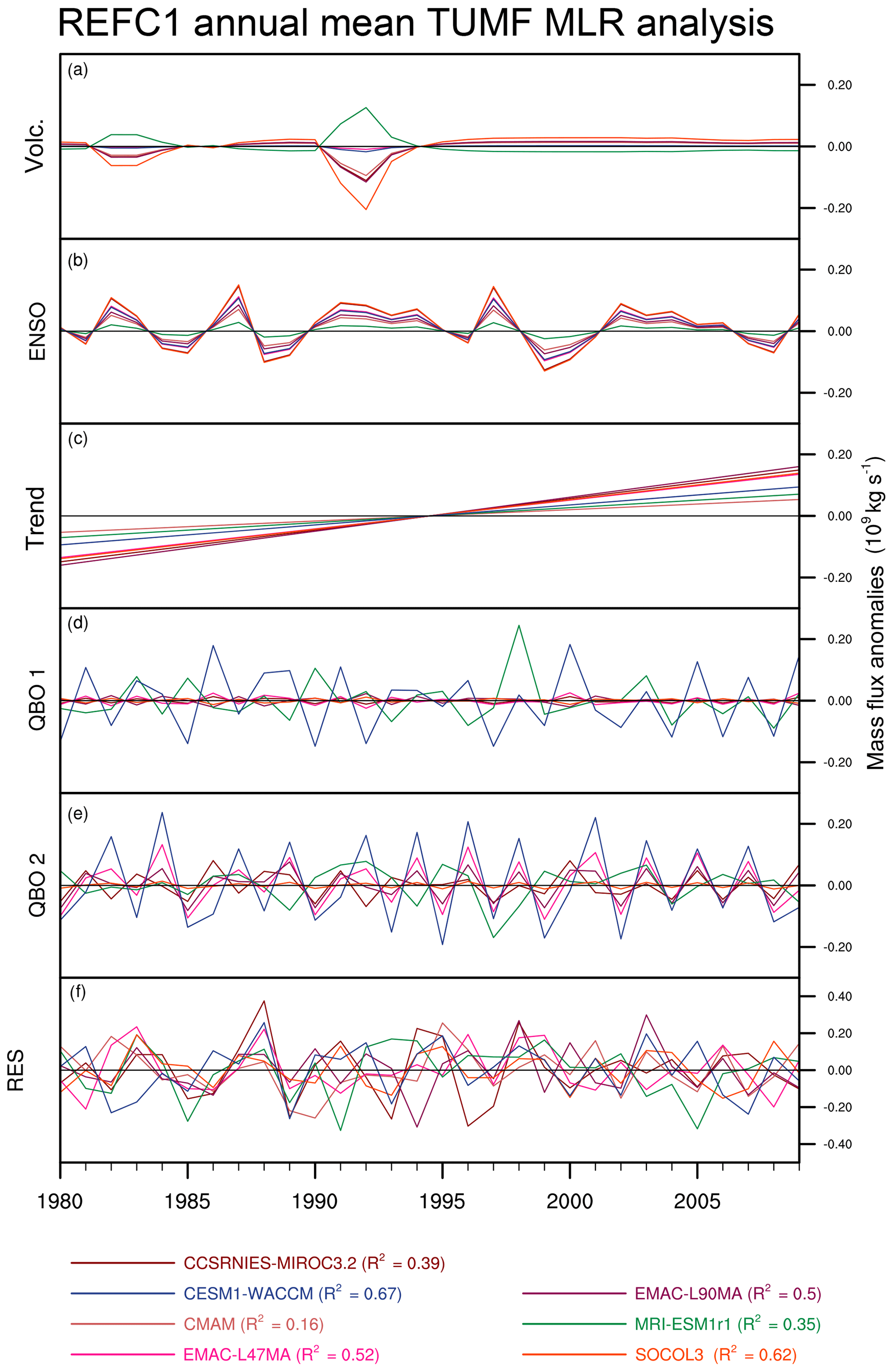
Figure 10Time series for REF-C1 simulations of the components of the annual mean tropical upward mass flux (×109 kg s−1) attributed to (a) volcanic aerosol, (b) ENSO, (c) linear trend, (d, e) QBO, and (f) regression residuals.
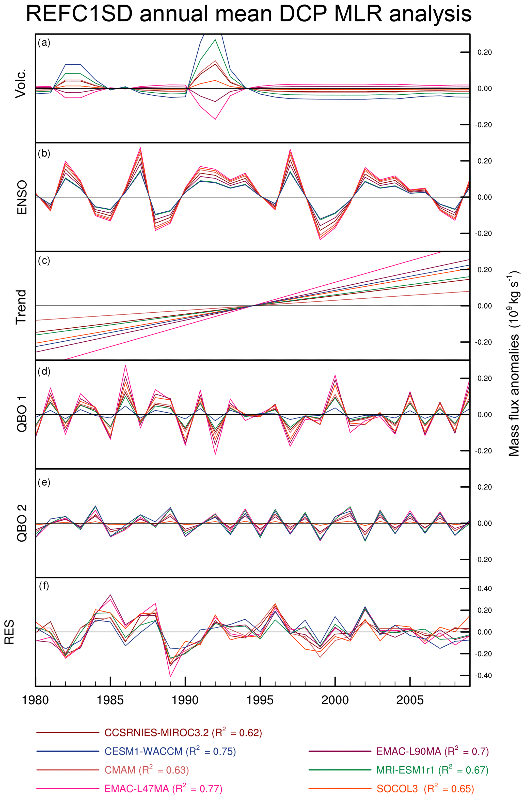
Figure 11Time series for REF-C1SD simulations of the components of the annual mean tropical upward mass flux (×109 kg s−1) attributed to (a) volcanic aerosol, (b) ENSO, (c) linear trend, (d, e) QBO, and (f) regression residuals.
The REF-C1 models all show a positive best-estimate regression coefficient for the TUMF response to ENSO (Fig. 10), which is quite consistent in amplitude, but it is only strongly statistically significant in CCSRNIES-MIROC3.2 and SOCOL3 (Fig. S5). This is in contrast to the REF-C1SD models, which all show a larger and more significant positive ENSO regression coefficient. The linear trend regression coefficient over 1980–2009 is positive in all REF-C1 models and is statistically significantly different from zero at the 95 % confidence level in five out of the seven models. The magnitude of the linear trend term varies by around a factor of 2 for REF-C1. In REF-C1SD, the amplitude of the linear trend regression coefficient increases in all models, but the intermodel spread increases to around a factor of 4. Hence, in these simulations nudging increases the disparity across models in the magnitude of the long-term TUMF trend.

Figure 12Tropical upward mass flux trends at 70 hPa (×109 kg s−1 decade−1) for different start (abscissa) and end (ordinate) dates over the period 1980–2009 for the REF-C1 (r1i1p1) simulations. Trends are not shown for periods of less than 10 years. Values with statistical significance greater than the 95 % level are shaded.
As expected, the variations in TUMF attributed to the QBO is quite different in the REF-C1 and REF-C1SD runs for those models that do not nudge the QBO in REF-C1, as shown in Figs. 10 and 11. The nudging of zonal winds in REF-C1SD constrains the phase of the QBO, and hence there is strikingly similar variability in the TUMF anomalies attributed to the QBO in the REF-C1SD runs.
The overall R2 values from the MLR model for the REF-C1 simulations vary between 0.16 (CMAM) and 0.67 (CESM1-WACCM). REF-C1SD runs generally give more consistent R2 values across the models, ranging from 0.62 (CCSRNIES-MIROC3.2) to 0.77 (EMAC-L47). This means that there is still a substantial fraction (>23 %) of unexplained variance in the annual TUMF time series in the REF-C1SD simulations after applying the MLR model, and the residuals exhibit a remarkable degree of temporal correlation. In contrast, the MLR residuals in the REF-C1 runs (Fig. 10f) show much less temporal coherence apart from a drop around 1989. The residuals in the REF-C1SD simulations (Fig. 11f) show a high degree of coherent inter-annual variability, another manifestation of the fact that the nudged runs do reproduce a much more consistent inter-annual variability. This makes a substantial contribution to the coherence of the TUMF time series in Fig. 9b, but it cannot be attributed to any of the terms included in the MLR model.
For completeness, the MLR model was also applied to the reanalysis TUMF at 70 hPa (Figs. S15 and S16). This highlights significant discrepancies in attributing the variance in TUMF in the different reanalysis datasets to the various basis functions in the MLR model. Both the volcanic activity and ENSO contributions to the variance in the TUMF are rather weak compared to the REF-C1SD runs. The negative linear trend in ERA-I is in strong contrast to the positive trends found in the other reanalyses and the REF-C1SD models. The negative trend in ERA-I found in the TUMF in the lower stratosphere over 1980–2009 corroborates the findings of Abalos et al. (2015), who showed a negative trend in the direct estimate in ERA-I over 1979–2012. Despite this difference in the representation of the long-term TUMF trend, ERA-I shows the highest percentage of TUMF variance explained by the MLR model (66 %), with MERRA showing a substantially lower R2 (0.3) compared to the other reanalyses and the REF-C1SD models. The residuals are generally less correlated between the reanalyses on inter-annual timescales than those found in the REF-C1SD simulations but are broadly similar on inter-decadal timescales. However, the regression residuals in the reanalyses show a different temporal behaviour from those in the REF-C1SD simulations (Fig. 11; note that the y-axis scale for the residuals in Fig. S15 is double that for the CCMI models in Figs. 10 and 11). In summary, although nudging constrains the inter-annual variability in the TUMF at 70 hPa, the attribution to some specific drivers differs across the models and, in comparison, to the reanalyses they were nudged towards.
3.6 Trend sensitivity analysis
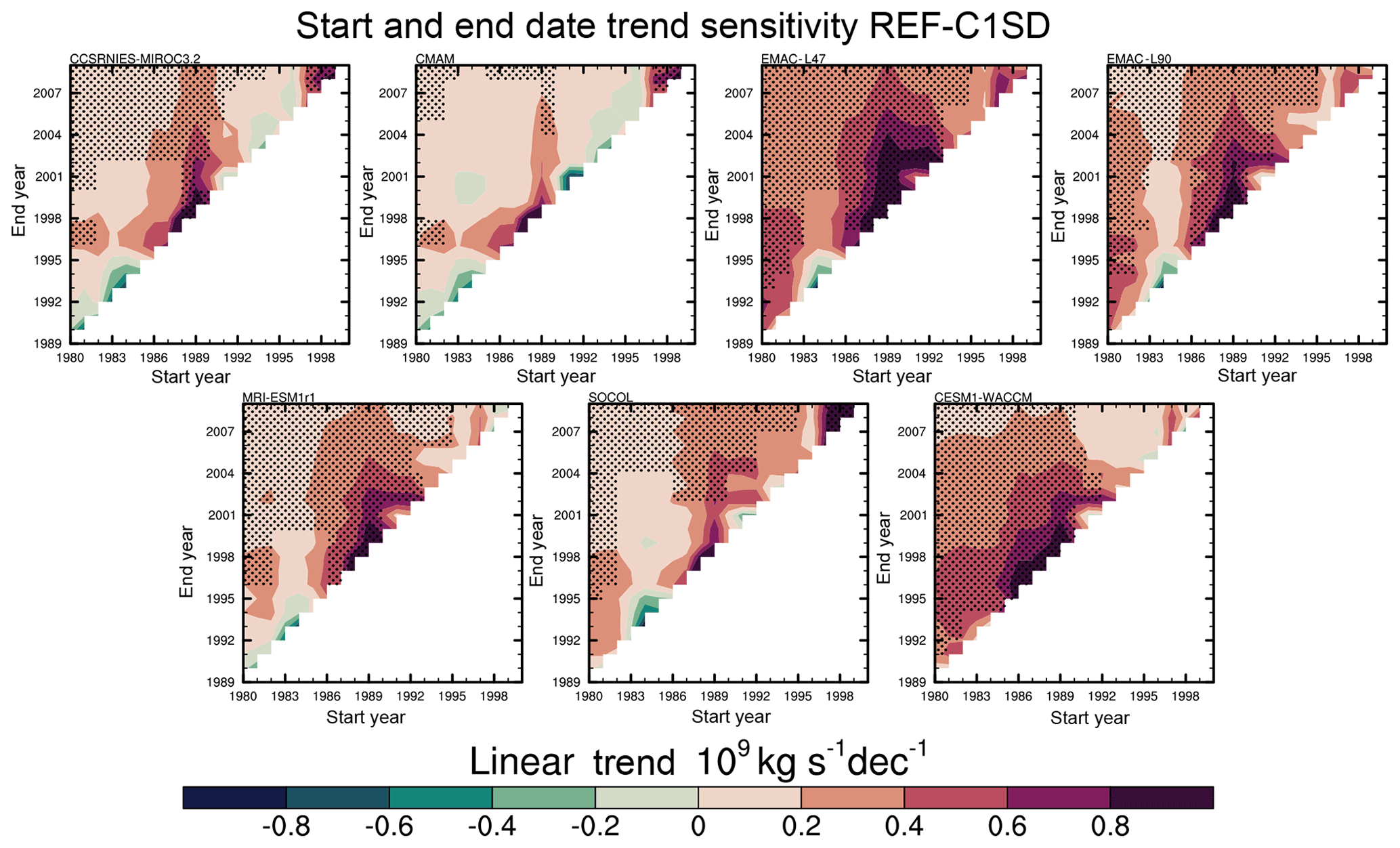
Following the results of the MLR analysis described in Sect. 3.5, which showed a statistically significant positive linear trend in most REF-C1 and REF-C1SD models for the 30-year period 1980–2009, we now explore the sensitivity of the linear trend to the time period considered. We apply the same MLR model as discussed in Sect. 3.5 to the annual mean 70 hPa TUMF time series of the first ensemble member for both REF-C1 and REF-C1SD runs as well as the reanalyses but systematically vary the start and end dates to cover all time periods in the window 1980–2009 that are at least 10 years in length. We then extract the linear trend coefficient from the MLR model and its associated p value. Figures 12 and 13 present the linear trend calculations for the REF-C1 and REF-C1SD runs, respectively, as a function of trend start and end date. The same trend sensitivity analysis for the reanalyses is presented in the Supplement (Fig. S17). Statistically significant trends at the 95 % confidence level are marked with black shading.
None of the periods considered in either the REF-C1 or REF-C1SD experiments show a significant negative TUMF trend. A statistically significant positive trend emerges in almost all of the REF-C1SD models for trends beginning in the mid-1980s to early 1990s extending to the mid-2000s. The trends are mainly significant for periods of 20 years or more and no less than around 12 years. This result broadly corroborates the findings of Hardiman et al. (2017a), who used a control run to estimate the period required to detect a BDC trend with an amplitude of 2 % per decade against the background internal variability. There is range of different structures in the diagnosed trends among models, particularly for the REF-C1 simulations, where a consistent pattern of positive trends only emerges across most models for the entire time period. This is because internal variability can mask BDC trends over short periods (Hardiman et al., 2017a). However, the REF-C1SD runs simulate more consistent variations in TUMF trends as a function of time period but generally show stronger positive trends than their free-running counterparts. Interestingly, the reanalysis trend sensitivity analysis highlights that nudging does not constrain the underlying trends of the REF-C1SD models in the TUMF at 70 hPa, as the reanalysis datasets exhibit a wide range of different trends from one another (Fig. S17) and differences compared to the trends in the REF-C1SD simulations (Fig. 13). For example, none of the REF-C1SD models simulate a statistically non-significant negative trend in TUMF, starting around mid-1990s up to 2009, as seen in all the reanalyses. However, it should also be noted that any trend combination starting around the end of 1990s in almost all cases of both REF-C1 and REF-C1SD runs exhibit no statistical significance possibly pointing towards the role of declining ODSs due to the implementation of the Montreal Protocol (Polvani et al., 2018).
This study has performed the first multi-model intercomparison of the impact of nudged meteorology on the representation of the stratospheric residual circulation. We use hindcast simulations over 1980–2009 from CCMI, with identical prescribed external forcings in two configurations: REF-C1SD with meteorological fields nudged towards reanalysis data (specified dynamics – SD) and REF-C1 that is free-running. The nudged simulations use one of three different reanalysis datasets (ERA-Interim, JRA-55, and MERRA), nudge different variables (u, v, T, vorticity, divergence, and surface pressure), and use different time constants to impose the additional nudging tendencies in the model equations.
The key findings of this study are as follows:
-
Nudging meteorology does not constrain the mean strength of the residual circulation compared to free-running simulations. In fact, for most of the metrics of the climatological residual circulation examined, including residual vertical velocities and mass fluxes, the inter-model spread is comparable or in some cases larger in the REF-C1SD simulations than in REF-C1.
-
Nudging leads to the models simulating on average stronger upwelling at the Equator in the lower stratosphere to middle stratosphere and a wider tropical pipe in the lower stratosphere. In most cases, the magnitude and structure of the climatological residual circulation in the REF-C1SD experiments differ markedly from those estimated for the reanalysis they are nudged towards.
-
In most of the nudged models there are large differences of up to 25 % between the directly calculated tropical upward mass flux in the lower stratosphere and that calculated from the diagnosed total wave forcing using the downward control principle (Haynes et al., 1991). However, the spread in the contributions from the resolved and parameterized wave forcing to the tropical mass flux is slightly reduced in the REF-C1SD simulations compared to REF-C1.
-
Despite the lack of agreement in the mean circulation, nudging tightly constrains the inter-annual variability in the tropical upward mass flux (TUMF) in the lower stratosphere. This is associated with constraints to the contributions from both the resolved and parameterized wave forcing despite the fact that the models use different reanalysis datasets for nudging. The reanalysis datasets themselves exhibit broadly similar inter-annual variability in TUMF in the lower stratosphere, albeit with different long-term trends.
-
A multiple linear regression (MLR) analysis shows that up to 77 % (67 %) of the inter-annual variance of the lower-stratospheric TUMF in the REF-C1SD (REF-C1) experiments can be explained by volcanic eruptions, ENSO, the QBO, and a linear trend. The remaining unexplained TUMF variance in the nudged models shows a high degree of a temporal coherence, but this is not the case for the free-running simulations.
-
The results of the MLR analysis applied to the TUMF in the reanalyses show differences in the total variance explained and the attribution of variance to the different physical proxies. There are also marked differences between the individual regression coefficients derived for the REF-C1SD models and the reanalysis dataset used for nudging.
-
Most nudged simulations show a statistically significant positive trend in TUMF in the lower stratosphere over 1980–2009, which is on average larger than the trends simulated in the free-running models. This is despite the fact that five out of the seven models analysed were nudged towards ERA-Interim, which shows a negative long-term trend in TUMF (see also Abalos et al., 2015), while JRA-55 and MERRA show a positive trend. However, the magnitude of the TUMF trend varies by up to a factor of 4 across the nudged models, which is larger than the spread in the free-running simulations. This is an important limitation for using nudged-CCM simulations to interpret long-term changes in stratospheric tracers.
-
A sensitivity analysis of the time period for calculating lower-stratospheric TUMF trends shows that a statistically significant (at the 95 % confidence level) positive trend in TUMF takes at least 12 years and in most cases around 20 years to emerge in the REF-C1SD runs. Despite the three reanalysis datasets showing different 30-year trends (1980–2009), they show a striking agreement in the statistically non-significant negative trends starting from the late 1990s up to 2009.
Our findings highlight that nudging strongly affects the representation of the stratospheric residual circulation in chemistry–climate model simulations, but it does not necessarily lead to improvements in the circulation. Similar disagreement in the characteristics of tropospheric transport in the CCMI nudged simulations has also been reported (Orbe et al., 2018). The differences found in the nudged runs compared with the free-running simulations suggest that although nudging horizontal fields can remove model biases in, for example, temperature and horizontal wind fields (Hardiman et al., 2017b), the simulated vertical wind field will not necessarily be similar to the reanalysis. A particularly interesting finding of our study is that while nudging does not constrain the mean strength of the residual circulation, it constrains the inter-annual variability. The reason for the distinct effects of nudging on the residual circulation across these different timescales is currently unknown.
Multiple factors are likely to determine the effect of nudging on the residual circulation in a given model, including model biases, nudging timescales, nudging parameters, nudging height range, and model resolution. The differences in the stratospheric residual circulation between the REF-C1SD and the REF-C1 runs may not arise solely from the dynamics but can also be partly influenced by the indirect effects of nudging the temperatures, which in turn affect the diabatic heating (Ming et al., 2016a, b). In addition to nudging the horizontal winds (mechanical nudging), nudging the temperature (thermal nudging) might be systematically creating a spurious heat source in the model, which leads to a stronger BDC in the lower stratosphere, as suggested by Miyazaki et al. (2005) with the MRI GCM. Our results highlight that in the method by which the large-scale flow is specified and more specifically the choice of the reanalysis fields, the relaxation timescale and the vertical grid (pressure level versus model level) in which the nudging is applied need to be better understood and evaluated for their influence on the stratospheric circulation. Discrepancies between the vertical grid of the models and the reanalysis pressure levels they are interpolated onto or unbalanced dynamics are possible explanations for the differences found between the directly inferred circulation and that diagnosed from the wave forcing in the nudged simulations. Nudging would either violate continuity, or if continuity is maintained, it will come at the expense of the vertical fluxes, which are not nudged. The interesting aspect here seems to be that this results in substantial change to the net fluxes across a range of timescales; i.e. it does not only increase numerical noise in the component. In order to reduce discrepancies between nudged and free-running simulations, various nudging techniques have been investigated. The role of gravity waves in the error growth that the nudging introduces over time has been highlighted for a single model (Smith et al., 2017). Constraining just the horizontal winds without the temperature was found to be a good strategy when investigating the aerosol indirect effects without affecting significantly the mean state (Zhang et al., 2014). The relaxation timescale when applying the nudging has been found to play an important role in single-model studies (Merryfield et al., 2013), but there is no general consensus for the value of the relaxation constant, which is specific to the model for the simulations considered here (Morgenstern et al., 2017). Given the varying implementations of nudging in the models analysed here, our study is ill-suited to investigate in detail the mechanisms for how nudging affects the residual circulation. A dedicated study of the sensitivities within one model to relaxation timescales, nudging parameters, nudging height range, and vertical resolution would help with offering a detailed explanation for these differences.
The large spread in climatological residual circulation in nudged-CCM simulations is an important limitation for those wishing to use them to examine tracer transport, for example in stratospheric ozone trends (Solomon et al., 2016), volcanic aerosols (Schmidt et al., 2018), and diagnostics for the age of air (Dietmüller et al., 2018). Despite the limitations for transport within the stratosphere described here, some success has been reported in studies that used nudged simulations to investigate specific meteorological events such as sudden stratospheric warmings and, in particular, for exploring processes beyond the top of the nudging region in the mesosphere–lower thermosphere (e.g. Tweedy et al., 2013; Chandran and Collins, 2014; Pedatella et al., 2014). In conclusion, owing to the limitations of the current techniques for nudging models highlighted here, we urge caution in drawing quantitative comparisons of stratospheric tracers affected by the residual circulation in nudged simulations against stratospheric observational data.
The majority of CCMI-1 data used in this study can be obtained through the British Atmospheric Data Centre (BADC) archive (ftp://ftp.ceda.ac.uk, last access: June 2018). For instructions for access to the archive, see http://blogs.reading.ac.uk/ccmi/badc-data-access (last access: July 2019). The correctly calculated EMAC-L47MA and EMAC-L90MA TEM model output for both REF-C1 and REF-C1SD was obtained directly from Hella Garny. The SOCOL3 REF-C1SD TEM model output was obtained from Andrea Stenke. The S-RIP data used in this study can be obtained through the BADC archive (ftp://ftp.ceda.ac.uk and http://dx.doi.org/10.5285/b241a7f536a244749662360bd7839312, last access: September 2018).
The supplement related to this article is available online at: https://doi.org/10.5194/acp-19-11559-2019-supplement.
AC performed the analysis and wrote the article. ACM and MPC designed the study and made substantial contributions to the interpretation of the data. Moreover, they participated in drafting and revising the paper. HG provided the correctly calculated EMAC data, and SD contributed to the discussion of the content. AS provided the SOCOL REF-C1SD data. The other co-authors contributed information pertaining to their individual models and helped edit the paper.
The authors declare that they have no conflict of interest.
This article is part of the special issue “Chemistry–Climate Modelling Initiative (CCMI) (ACP/AMT/ESSD/GMD inter-journal SI)”. It is not associated with a conference.
Andreas Chrysanthou was supported by a University of Leeds Anniversary Postgraduate Scholarship. Amanda C. Maycock was supported by a NERC Independent Research Fellowship (grant NE/M018199/1). Martyn P. Chipperfield and Sandip Dhomse acknowledge support through the NERC SISLAC grant NE/R001782/1. We acknowledge the modelling groups for making their simulations available for this analysis, the joint WCRP SPARC–IGAC Chemistry–Climate Model Initiative (CCMI) for organizing and coordinating the model data analysis activity, and the British Atmospheric Data Centre (BADC) for collecting and archiving the CCMI model output. The EMAC simulations have been performed at the German Climate Computing Centre (DKRZ) through support from the Bundesministerium für Bildung und Forschung (BMBF). DKRZ and its scientific steering committee are gratefully acknowledged for providing the HPC and data archiving resources for this consortial project ESCiMo (Earth System Chemistry Integrated Modelling). CCSRNIES research was supported by the Environment Research and Technology Development Fund (2-1303 and 2-1709) of the Ministry of the Environment of Japan and a grant in aid for scientific research from the Ministry of Education, Culture, Sports, Science and Technology (MEXT) of Japan (16H01183 and 18KK0289), and computations were performed on NEC SX9/A(ECO) and NEC SXACE computers at the CGER, NIES. The GEOSCCM is supported by the NASA MAP programme, and the high-performance computing resources were provided by the NASA Center for Climate Simulation (NCCS). The analysis and visualization of the study were performed using the NCAR Command Language (NCL). The authors wish to acknowledge the contribution of Olaf Morgenstern and Guang Zeng in the discussion of the paper specifically for the model results of NIWA-UKCA in this research.
This research has been supported by the Natural Environment Research Council (grant nos. NE/M018199/1 and NE/R001782/1).
This paper was edited by William Ward and reviewed by two anonymous referees.
Abalos, M., Legras, B., Ploeger, F., and Randel, W. J.: Evaluating the advective Brewer-Dobson circulation in three reanalyses for the period 1979–2012, J. Geophys. Res., 120, 7534–7554, https://doi.org/10.1002/2015JD023182, 2015.
Abalos, M., Polvani, L., Calvo, N., Kinnison, D., Ploeger, F., Randel, W., and Solomon, S.: New Insights on the Impact of Ozone-Depleting Substances on the Brewer-Dobson Circulation, J. Geophys. Res.-Atmos., 124, 2435–2451, https://doi.org/10.1029/2018JD029301, 2019.
Akiyoshi, H., Nakamura, T., Miyasaka, T., Shiotani, M., and Suzuki, M.: A nudged chemistry-climate model simulation of chemical constituent distribution at northern high-latitude stratosphere observed by SMILES and MLS during the 2009/2010 stratospheric sudden warming, J. Geophys. Res.-Atmos., 121, 1361–1380, https://doi.org/10.1002/2015JD023334, 2016.
Andrews, D. G. and McIntyre, M. E.: Planetary Waves in Horizontal and Vertical Shear: The Generalized Eliassen-Palm Relation and the Mean Zonal Acceleration, J. Atmos. Sci., 33, 2031–2048, https://doi.org/10.1175/1520-0469(1976)033<2031:pwihav>2.0.co;2, 1976.
Andrews, D. G. and Mcintyre, M. E.: An exact theory of nonlinear waves on a Lagrangian-mean flow, J. Fluid Mech., 89, 609–646, https://doi.org/10.1017/S0022112078002773, 1978.
Andrews, D. G., Holton, J. R., and Leovy, C. B.: Middle Atmosphere Dynamics, International Geophysical Series, Vol. 40, 1987.
Baldwin, M. P., Gray, L. J., Dunkerton, T. J., Hamilton, K., Haynes, P. H., Randel, W. J., Holton, J. R., Alexander, M. J., Hirota, I., Horinouchi, T., Jones, D. B. A., Kinnersley, J. S., Marquardt, C., Sato, K., and Takahashi, M.: The quasi-biennial oscillation, Rev. Geophys., 39, 179–229, https://doi.org/10.1029/1999RG000073, 2001.
Ball, W. T., Alsing, J., Mortlock, D. J., Staehelin, J., Haigh, J. D., Peter, T., Tummon, F., Stübi, R., Stenke, A., Anderson, J., Bourassa, A., Davis, S. M., Degenstein, D., Frith, S., Froidevaux, L., Roth, C., Sofieva, V., Wang, R., Wild, J., Yu, P., Ziemke, J. R., and Rozanov, E. V.: Evidence for a continuous decline in lower stratospheric ozone offsetting ozone layer recovery, Atmos. Chem. Phys., 18, 1379–1394, https://doi.org/10.5194/acp-18-1379-2018, 2018.
Beres, J. H., Garcia, R. R., Boville, B. A., and Sassi, F.: Implementation of a gravity wave source spectrum parameterization dependent on the properties of convection in the Whole Atmosphere Community Climate Model (WACCM), J. Geophys. Res.-Atmos., 110, 1–13, https://doi.org/10.1029/2004JD005504, 2005.
Birner, T. and Bönisch, H.: Residual circulation trajectories and transit times into the extratropical lowermost stratosphere, Atmos. Chem. Phys., 11, 817–827, https://doi.org/10.5194/acp-11-817-2011, 2011.
Butchart, N.: The Brewer-Dobson circulation, Rev. Geophys., 52, 157–184, https://doi.org/10.1002/2013RG000448, 2014.
Butchart, N. and Scaife, A. A.: Removal of chlorofluorocarbons by increased mass exchange between the stratosphere and troposphere in a changing climate, Nature, 410, 799–802, https://doi.org/10.1038/35071047, 2001.
Butchart, N., Scaife, A. A., Bourqui, M., Grandpré, J., Hare, S. H. E., Kettleborough, J., Langematz, U., Manzini, E., Sassi, F., Shibata, K., Shindell, D., and Sigmond, M.: Simulations of anthropogenic change in the strength of the Brewer-Dobson circulation, Clim. Dynam., 27, 727–741, https://doi.org/10.1007/s00382-006-0162-4, 2006.
Butchart, N., Cionni, I., Eyring, V., Shepherd, T. G., Waugh, D. W., Akiyoshi, H., Austin, J., Brühl, C., Chipperfield, M. P., Cordero, E., Dameris, M., Deckert, R., Dhomse, S., Frith, S. M., Garcia, R. R., Gettelman, A., Giorgetta, M. A., Kinnison, D. E., Li, F., Mancini, E., Mclandress, C., Pawson, S., Pitari, G., Plummer, D. A., Rozanov, E., Sassi, F., Scinocca, J. F., Shibata, K., Steil, B., and Tian, W.: Chemistry-climate model simulations of twenty-first century stratospheric climate and circulation changes, J. Climate, 23, 5349–5374, https://doi.org/10.1175/2010JCLI3404.1, 2010.
Butchart, N., Charlton-Perez, A. J., Cionni, I., Hardiman, S. C., Haynes, P. H., Krüger, K., Kushner, P. J., Newman, P. A., Osprey, S. M., Perlwitz, J., Sigmond, M., Wang, L., Akiyoshi, H., Austin, J., Bekki, S., Baumgaertner, A., Braesicke, P., Brhl, C., Chipperfield, M., Dameris, M., Dhomse, S., Eyring, V., Garcia, R., Garny, H., Jöckel, P., Lamarque, J. F., Marchand, M., Michou, M., Morgenstern, O., Nakamura, T., Pawson, S., Plummer, D., Pyle, J., Rozanov, E., Scinocca, J., Shepherd, T. G., Shibata, K., Smale, D., Teyssèdre, H., Tian, W., Waugh, D., and Yamashita, Y.: Multimodel climate and variability of the stratosphere, J. Geophys. Res.-Atmos., 116, 1–21, https://doi.org/10.1029/2010JD014995, 2011.
Calvo, N., Garcia, R. R., Randel, W. J., and Marsh, D. R.: Dynamical Mechanism for the Increase in Tropical Upwelling in the Lowermost Tropical Stratosphere during Warm ENSO Events, J. Atmos. Sci., 67, 2331–2340, https://doi.org/10.1175/2010jas3433.1, 2010.
Chandran, A. and Collins, R. L.: Stratospheric sudden warming effects on winds and temperature in the middle atmosphere at middle and low latitudes: a study using WACCM, Ann. Geophys., 32, 859–874, https://doi.org/10.5194/angeo-32-859-2014, 2014.
Chipperfield, M. P.: Multiannual simulations with a three-dimensional chemical transport model, J. Geophys. Res.-Atmos., 104, 1781–1805, https://doi.org/10.1029/98JD02597, 1999.
Chipperfield, M. P.: New version of the TOMCAT/SLIMCAT off-line chemical transport model: Intercomparison of stratospheric tracer experiments, Q. J. Roy. Meteor. Soc., 132, 1179–1203, https://doi.org/10.1256/qj.05.51, 2006.
Chipperfield, M. P., Cariolle, D., and Simon, P.: A 3D transport model study of chlorine activation during EASOE, Geophys. Res. Lett., 21, 1467–1470, https://doi.org/10.1029/93GL01679, 1994.
Chipperfield, M. P., Dhomse, S., Hossaini, R., Feng, W., Santee, M. L., Weber, M., Burrows, J. P., Wild, J. D., Loyola, D., and Coldewey-Egbers, M.: On the Cause of Recent Variations in Lower Stratospheric Ozone, Geophys. Res. Lett., 45, 5718–5726, https://doi.org/10.1029/2018GL078071, 2018.
Cohen, N. Y., Gerber, E. P., and Bühler, O.: Compensation between Resolved and Unresolved Wave Driving in the Stratosphere: Implications for Downward Control, J. Atmos. Sci., 70, 3780–3798, https://doi.org/10.1175/jas-d-12-0346.1, 2013.
Dee, D. P., Uppala, S. M., Simmons, A. J., Berrisford, P., Poli, P., Kobayashi, S., Andrae, U., Balmaseda, M. A., Balsamo, G., Bauer, P., Bechtold, P., Beljaars, A. C. M., van de Berg, L., Bidlot, J., Bormann, N., Delsol, C., Dragani, R., Fuentes, M., Geer, A. J., Haimberger, L., Healy, S. B., Hersbach, H., Hólm, E. V., Isaksen, L., Kållberg, P., Köhler, M., Matricardi, M., Mcnally, A. P., Monge-Sanz, B. M., Morcrette, J. J., Park, B. K., Peubey, C., de Rosnay, P., Tavolato, C., Thépaut, J. N., and Vitart, F.: The ERA-Interim reanalysis: Configuration and performance of the data assimilation system, Q. J. Roy. Meteor. Soc., 137, 553–597, https://doi.org/10.1002/qj.828, 2011.
Deushi, M. and Shibata, K.: Development of a Meteorological Research Institute chemistry-climate model version 2 for the study of tropospheric and stratospheric chemistry, Pap. Meteorol. Geophys., 62, 1–46, https://doi.org/10.2467/mripapers.62.1, 2011.
Diallo, M., Ploeger, F., Konopka, P., Birner, T., Müller, R., Riese, M., Garny, H., Legras, B., Ray, E., Berthet, G., and Jegou, F.: Significant Contributions of Volcanic Aerosols to Decadal Changes in the Stratospheric Circulation, Geophys. Res. Lett., 44, 10780–10791, https://doi.org/10.1002/2017GL074662, 2017.
Dietmüller, S., Garny, H., Plöger, F., Jöckel, P., and Cai, D.: Effects of mixing on resolved and unresolved scales on stratospheric age of air, Atmos. Chem. Phys., 17, 7703–7719, https://doi.org/10.5194/acp-17-7703-2017, 2017.
Dietmüller, S., Eichinger, R., Garny, H., Birner, T., Boenisch, H., Pitari, G., Mancini, E., Visioni, D., Stenke, A., Revell, L., Rozanov, E., Plummer, D. A., Scinocca, J., Jöckel, P., Oman, L., Deushi, M., Kiyotaka, S., Kinnison, D. E., Garcia, R., Morgenstern, O., Zeng, G., Stone, K. A., and Schofield, R.: Quantifying the effect of mixing on the mean age of air in CCMVal-2 and CCMI-1 models, Atmos. Chem. Phys., 18, 6699–6720, https://doi.org/10.5194/acp-18-6699-2018, 2018.
Douville, H.: Stratospheric polar vortex influence on Northern Hemisphere winter climate variability, Geophys. Res. Lett., 36, 1–5, https://doi.org/10.1029/2009GL039334, 2009.
Ebita, A., Kobayashi, S., Ota, Y., Moriya, M., Kumabe, R., Onogi, K., Harada, Y., Yasui, S., Miyaoka, K., Takahashi, K., Kamahori, H., Kobayashi, C., Endo, H., Soma, M., Oikawa, Y., and Ishimizu, T.: The Japanese 55-year Reanalysis “JRA-55”: An Interim Report, Sola, 7, 149–152, https://doi.org/10.2151/sola.2011-038, 2011.
Eichinger, R., Dietmüller, S., Garny, H., Šácha, P., Birner, T., Bönisch, H., Pitari, G., Visioni, D., Stenke, A., Rozanov, E., Revell, L., Plummer, D. A., Jöckel, P., Oman, L., Deushi, M., Kinnison, D. E., Garcia, R., Morgenstern, O., Zeng, G., Stone, K. A., and Schofield, R.: The influence of mixing on the stratospheric age of air changes in the 21st century, Atmos. Chem. Phys., 19, 921–940, https://doi.org/10.5194/acp-19-921-2019, 2019.
Engel, A., Möbius, T., Bönisch, H., Schmidt, U., Heinz, R., Levin, I., Atlas, E., Aoki, S., Nakazawa, T., Sugawara, S., Moore, F., Hurst, D., Elkins, J., Schauffler, S., Andrews, A., and Boering, K.: Age of stratospheric air unchanged within uncertainties over the past 30 years, Nat. Geosci., 2, 28–31, https://doi.org/10.1038/ngeo388, 2009.
Engel, A., Bönisch, H., Ullrich, M., Sitals, R., Membrive, O., Danis, F., and Crevoisier, C.: Mean age of stratospheric air derived from AirCore observations, Atmos. Chem. Phys., 17, 6825–6838, https://doi.org/10.5194/acp-17-6825-2017, 2017.
Eyring, V., Lamarque, J.-F., Cionni, I., Duncan, B., Fiore, A., Gettel-Man, A., Hegglin, M., Hess, P., Nagashima, T., Ryerson, T., Shepherd, T., Shindell, D., Waugh, D., and Young, P.: Report on the IGAC/SPARC Chemistry-Climate Model Initiative (CCMI) 2013 Science Workshop, available at: https://www.sparc-climate.org/publications/newsletter/ (last access: 15 July 2019), 2013.
Froidevaux, L., Kinnison, D. E., Wang, R., Anderson, J., and Fuller, R. A.: Evaluation of CESM1 (WACCM) free-running and specified dynamics atmospheric composition simulations using global multispecies satellite data records, Atmos. Chem. Phys., 19, 4783–4821, https://doi.org/10.5194/acp-19-4783-2019, 2019.
García-Herrera, R., Calvo, N., Garcia, R. R., and Giorgetta, M. A.: Propagation of ENSO temperature signals into the middle atmosphere: A comparison of two general circulation models and ERA-40 reanalysis data, J. Geophys. Res.-Atmos., 111, 1–14, https://doi.org/10.1029/2005JD006061, 2006.
Garcia, R. R. and Boville, B. A.: “Downward Control” of the Mean Meridional Circulation and Temperature Distribution of the Polar Winter Stratosphere, J. Atmos. Sci., 51, 2238–2245, https://doi.org/10.1175/1520-0469(1994)051<2238:COTMMC>2.0.CO;2, 1994.
Garcia, R. R., Randel, W. J., and Kinnison, D. E.: On the Determination of Age of Air Trends from Atmospheric Trace Species, J. Atmos. Sci., 68, 139–154, https://doi.org/10.1175/2010jas3527.1, 2010.
Garcia, R. R., Smith, A. K., Kinnison, D. E., Cámara, Á. de la, and Murphy, D. J.: Modification of the Gravity Wave Parameterization in the Whole Atmosphere Community Climate Model: Motivation and Results, J. Atmos. Sci., 74, 275–291, https://doi.org/10.1175/jas-d-16-0104.1, 2016.
Garny, H., Birner, T., Bönisch, H., and Bunzel, F.: The effects of mixing on age of air, J. Geophys. Res., 119, 7015–7034, https://doi.org/10.1002/2013JD021417, 2014.
Haenel, F. J., Stiller, G. P., von Clarmann, T., Funke, B., Eckert, E., Glatthor, N., Grabowski, U., Kellmann, S., Kiefer, M., Linden, A., and Reddmann, T.: Reassessment of MIPAS age of air trends and variability, Atmos. Chem. Phys., 15, 13161–13176, https://doi.org/10.5194/acp-15-13161-2015, 2015.
Hardiman, S. C., Butchart, N., and Calvo, N.: The morphology of the Brewer-Dobson circulation and its response to climate change in CMIP5 simulations, Q. J. Roy. Meteor. Soc., 140, 1958–1965, https://doi.org/10.1002/qj.2258, 2014.
Hardiman, S. C., Lin, P., Scaife, A. A., Dunstone, N. J., and Ren, H. L.: The influence of dynamical variability on the observed Brewer-Dobson circulation trend, Geophys. Res. Lett., 44, 2885–2892, https://doi.org/10.1002/2017GL072706, 2017a.
Hardiman, S. C., Butchart, N., O'Connor, F. M., and Rumbold, S. T.: The Met Office HadGEM3-ES chemistry–climate model: evaluation of stratospheric dynamics and its impact on ozone, Geosci. Model Dev., 10, 1209–1232, https://doi.org/10.5194/gmd-10-1209-2017, 2017b.
Haynes, P. H., McIntyre, M. E., Shepherd, T. G., Marks, C. J., and Shine, K. P.: On the “Downward Control” of Extratropical Diabatic Circulations by Eddy-Induced Mean Zonal Forces, J. Atmos. Sci., 48, 651–678, https://doi.org/10.1175/1520-0469(1991)048<0651:OTCOED>2.0.CO;2, 1991.
Hegglin, M. I. and Lamarque, J. F.: The IGAC/SPARC Chemistry-Climate Model Initiative Phase-1 (CCMI-1) model data output. NCAS British Atmospheric Data Centre, available at: https://catalogue.ceda.ac.uk/uuid/9cc6b94df0f4469d8066d69b5df879d5 (last access: 6 June 2018), 2015.
Hegglin, M. I. and Shepherd, T. G.: Large climate-induced changes in ultraviolet index and stratosphere-to- troposphere ozone flux, Nat. Geosci., 2, 687–691, https://doi.org/10.1038/ngeo604, 2009.
Hines, C. O.: Doppler-spread parameterization of gravity-wave momentum deposition in the middle atmosphere. Part 1: Basic formulation, J. Atmos. Sol.-Terr. Phy., 59, 371–386, https://doi.org/10.1016/S1364-6826(96)00079-X, 1997a.
Hines, C. O.: Doppler-spread parameterization of gravity-wave momentum deposition in the middle atmosphere. Part 2: Broad and quasi monochromatic spectra, and implementation, J. Atmos. Sol.-Terr. Phy., 59, 387–400, https://doi.org/10.1016/s1364-6826(96)00080-6, 1997b.
Hitchcock, P. and Simpson, I. R.: The Downward Influence of Stratospheric Sudden Warmings*, J. Atmos. Sci., 71, 3856–3876, https://doi.org/10.1175/jas-d-14-0012.1, 2014.
Holton, J. R., Haynes, P. H., McIntyre, M. E., Douglass, A. R., Rood, R. B., and Pfister, L.: Stratosphere-troposphere exchange, Rev. Geophys., 33, 403–439, https://doi.org/10.1029/95RG02097, 1995.
Imai, K., Manago, N., Mitsuda, C., Naito, Y., Nishimoto, E., Sakazaki, T., Fujiwara, M., Froidevaux, L., Von Clarmann, T., Stiller, G. P., Murtagh, D. P., Rong, P. P., Mlynczak, M. G., Walker, K. A., Kinnison, D. E., Akiyoshi, H., Nakamura, T., Miyasaka, T., Nishibori, T., Mizobuchi, S., Kikuchi, K. I., Ozeki, H., Takahashi, C., Hayashi, H., Sano, T., Suzuki, M., Takayanagi, M., and Shiotani, M.: Validation of ozone data from the Superconducting Submillimeter-Wave Limb-Emission Sounder (SMILES), J. Geophys. Res.-Atmos., 118, 5750–5769, https://doi.org/10.1002/jgrd.50434, 2013.
Jeuken, A. B. M., Siegmund, P. C., Heijboer, L. C., Feichter, J., and Bengtsson, L.: On the potential of assimilating meteorological analyses in a global climate model for the purpose of model validation, J. Geophys. Res.-Atmos., 101, 16939–16950, https://doi.org/10.1029/96JD01218, 1996.
Jöckel, P., von Kuhlmann, R., Lawrence, M. G., Steil, B., Brenninkmeijer, C. A. M., Crutzen, P. J., Rasch, P. J., and Eaton, B.: On a fundamental problem in implementing flux-form advection schemes for tracer transport in 3-dimensional general circulation and chemistry transport models, Q. J. Roy. Meteor. Soc., 127, 1035–1052, https://doi.org/10.1256/smsqj.57317, 2001.
Jöckel, P., Kerkweg, A., Pozzer, A., Sander, R., Tost, H., Riede, H., Baumgaertner, A., Gromov, S., and Kern, B.: Development cycle 2 of the Modular Earth Submodel System (MESSy2), Geosci. Model Dev., 3, 717–752, https://doi.org/10.5194/gmd-3-717-2010, 2010.
Jöckel, P., Tost, H., Pozzer, A., Kunze, M., Kirner, O., Brenninkmeijer, C. A. M., Brinkop, S., Cai, D. S., Dyroff, C., Eckstein, J., Frank, F., Garny, H., Gottschaldt, K.-D., Graf, P., Grewe, V., Kerkweg, A., Kern, B., Matthes, S., Mertens, M., Meul, S., Neumaier, M., Nützel, M., Oberländer-Hayn, S., Ruhnke, R., Runde, T., Sander, R., Scharffe, D., and Zahn, A.: Earth System Chemistry integrated Modelling (ESCiMo) with the Modular Earth Submodel System (MESSy) version 2.51, Geosci. Model Dev., 9, 1153–1200, https://doi.org/10.5194/gmd-9-1153-2016, 2016.
Jonsson, A. I., de Grandpré, J., Fomichev, V. I., McConnell, J. C., and Beagley, S. R.: Doubled CO2-induced cooling in the middle atmosphere: Photochemical analysis of the ozone radiative feedback, J. Geophys. Res.-Atmos., 109, 1–18, https://doi.org/10.1029/2004JD005093, 2004.
Jung, T., Miller, M. J., and Palmer, T. N.: Diagnosing the Origin of Extended-Range Forecast Errors, Mon. Weather Rev., 138, 2434–2446, https://doi.org/10.1175/2010mwr3255.1, 2010.
Karpechko, A. Y. and Maycock, A. C. (Lead Authors), Abalos, M., Akiyoshi, H., Arblaster, J. M., Garfinkel, C. I., Rosenlof, K. H., and Sigmond, M.: Stratospheric Ozone Changes and Climate, Chapter 5 in Scientific Assessment of Ozone Depletion: 2018, Global Ozone Research and Monitoring Project – Report No. 58, World Meteorological Organization, Geneva, Switzerland, 2018.
Keeble, J., Bednarz, E. M., Banerjee, A., Abraham, N. L., Harris, N. R. P., Maycock, A. C., and Pyle, J. A.: Diagnosing the radiative and chemical contributions to future changes in tropical column ozone with the UM-UKCA chemistry–climate model, Atmos. Chem. Phys., 17, 13801–13818, https://doi.org/10.5194/acp-17-13801-2017, 2017.
Kida, H.: General Circulation of Air Parcels and Transport Characteristics Derived from a hemispheric GCM, J. Meteorol. Soc. Jpn. Ser. II, 61, 171–187, https://doi.org/10.2151/jmsj1965.61.2_171, 1983.
Kobayashi, C. and Iwasaki, T.: Brewer-Dobson circulation diagnosed from JRA-55, J. Geophys. Res., 121, 1493–1510, https://doi.org/10.1002/2015JD023476, 2016.
Kobayashi, S., Ota, Y., Harada, Y., Ebita, A., Moriya, M., Onoda, H., Onogi, K., Kamahori, H., Kobayashi, C., Endo, H., Miyaoka, K., and Takahashi, K.: The JRA-55 Reanalysis: General Specifications and Basic Characteristics, J. Meteorol. Soc. Jpn. Ser. II, 93, 5–48, https://doi.org/10.2151/jmsj.2015-001, 2015.
Krol, M., de Bruine, M., Killaars, L., Ouwersloot, H., Pozzer, A., Yin, Y., Chevallier, F., Bousquet, P., Patra, P., Belikov, D., Maksyutov, S., Dhomse, S., Feng, W., and Chipperfield, M. P.: Age of air as a diagnostic for transport timescales in global models, Geosci. Model Dev., 11, 3109–3130, https://doi.org/10.5194/gmd-11-3109-2018, 2018.
Lamarque, J.-F., Emmons, L. K., Hess, P. G., Kinnison, D. E., Tilmes, S., Vitt, F., Heald, C. L., Holland, E. A., Lauritzen, P. H., Neu, J., Orlando, J. J., Rasch, P. J., and Tyndall, G. K.: CAM-chem: description and evaluation of interactive atmospheric chemistry in the Community Earth System Model, Geosci. Model Dev., 5, 369–411, https://doi.org/10.5194/gmd-5-369-2012, 2012.
Lamarque, J.-F., Shindell, D. T., Josse, B., Young, P. J., Cionni, I., Eyring, V., Bergmann, D., Cameron-Smith, P., Collins, W. J., Doherty, R., Dalsoren, S., Faluvegi, G., Folberth, G., Ghan, S. J., Horowitz, L. W., Lee, Y. H., MacKenzie, I. A., Nagashima, T., Naik, V., Plummer, D., Righi, M., Rumbold, S. T., Schulz, M., Skeie, R. B., Stevenson, D. S., Strode, S., Sudo, K., Szopa, S., Voulgarakis, A., and Zeng, G.: The Atmospheric Chemistry and Climate Model Intercomparison Project (ACCMIP): overview and description of models, simulations and climate diagnostics, Geosci. Model Dev., 6, 179–206, https://doi.org/10.5194/gmd-6-179-2013, 2013.
Lefèvre, F., Brasseur, G. P., Folkins, I., Smith, A. K., and Simon, P.: Chemistry of the 1991–1992 stratospheric winter: three-dimensional model simulations, J. Geophys. Res., 99, 8183–8195, https://doi.org/10.1029/93JD03476, 1994.
Li, F., Newman, P., Pawson, S., and Perlwitz, J.: Effects of Greenhouse Gas Increase and Stratospheric Ozone Depletion on Stratospheric Mean Age of Air in 1960–2010, J. Geophys. Res.-Atmos., 123, 2098–2110, https://doi.org/10.1002/2017JD027562, 2018.
Linz, M., Plumb, R. A., Gerber, E. P., Haenel, F. J., Stiller, G., Kinnison, D. E., Ming, A., and Neu, J. L.: The strength of the meridional overturning circulation of the stratosphere, Nat. Geosci., 10, 663–667, https://doi.org/10.1038/ngeo3013, 2017.
Linz, M., Abalos, M., Glanville, A. S., Kinnison, D. E., Ming, A., and Neu, J. L.: The global diabatic circulation of the stratosphere as a metric for the Brewer–Dobson circulation, Atmos. Chem. Phys., 19, 5069–5090, https://doi.org/10.5194/acp-19-5069-2019, 2019.
Löffler, M., Brinkop, S., and Jöckel, P.: Impact of major volcanic eruptions on stratospheric water vapour, Atmos. Chem. Phys., 16, 6547–6562, https://doi.org/10.5194/acp-16-6547-2016, 2016.
Mahieu, E., Chipperfield, M. P., Notholt, J., Reddmann, T., Anderson, J., Bernath, P. F., Blumenstock, T., Coffey, M. T., Dhomse, S. S., Feng, W., Franco, B., Froidevaux, L., Griffith, D. W. T., Hannigan, J. W., Hase, F., Hossaini, R., Jones, N. B., Morino, I., Murata, I., Nakajima, H., Palm, M., Paton-Walsh, C., Russell, J. M., Schneider, M., Servais, C., Smale, D., and Walker, K. A.: Recent Northern Hemisphere stratospheric HCl increase due to atmospheric circulation changes, Nature, 515, 104–107, https://doi.org/10.1038/nature13857, 2014.
Marsh, D. R. and Garcia, R. R.: Attribution of decadal variability in lower-stratospheric tropical ozone, Geophys. Res. Lett., 34, 1–5, https://doi.org/10.1029/2007GL030935, 2007.
Marsh, D. R., Mills, M. J., Kinnison, D. E., Lamarque, J. F., Calvo, N., and Polvani, L. M.: Climate change from 1850 to 2005 simulated in CESM1(WACCM), J. Climate, 26, 7372–7391, https://doi.org/10.1175/JCLI-D-12-00558.1, 2013.
Martineau, P.: S-RIP: Zonal-mean dynamical variables of global atmospheric reanalyses on pressure levels, Centre for Environmental Data Analysis, https://doi.org/10.5285/b241a7f536a244749662360bd7839312, 2017.
Martineau, P., Wright, J. S., Zhu, N., and Fujiwara, M.: Zonal-mean data set of global atmospheric reanalyses on pressure levels, Earth Syst. Sci. Data, 10, 1925–1941, https://doi.org/10.5194/essd-10-1925-2018, 2018.
Maycock, A. C., Randel, W. J., Steiner, A. K., Karpechko, A. Y., Cristy, J., Saunders, R., Thompson, D. W. J., Zou, C.-Z., Chrysanthou, A., Abraham, N. L., Akiyoshi, H., Archibald, A. T., Butchart, N., Chipperfield, M., Dameris, M., Deushi, M., Dhomse, S., Di Genova, G., Jöckel, P., Kinnison, D. E., Kirner, O., Ladstädter, F., Michou, M., Morgenstern, O., O'Connor, F., Oman, L., Pitari, G., Plummer, D. A., Revell, L. E., Rozanov, E., Stenke, A., Visioni, D., Yamashita, Y., and Zeng, G.: Revisiting the mystery of recent stratospheric temperature trends, Geophys. Res. Lett., 1–15, https://doi.org/10.1029/2018GL078035, 2018.
McLandress, C., Scinocca, J. F., Shepherd, T. G., Reader, M. C., and Manney, G. L.: Dynamical Control of the Mesosphere by Orographic and Nonorographic Gravity Wave Drag during the Extended Northern Winters of 2006 and 2009, J. Atmos. Sci., 70, 2152–2169, https://doi.org/10.1175/JAS-D-12-0297.1, 2013.
Merryfield, W. J., Lee, W. S., Boer, G. J., Kharin, V. V., Scinocca, J. F., Flato, G. M., Ajayamohan, R. S., Fyfe, J. C., Tang, Y., and Polavarapu, S.: The canadian seasonal to interannual prediction system. part I: Models and initialization, Mon. Weather Rev., 141, 2910–2945, https://doi.org/10.1175/MWR-D-12-00216.1, 2013.
Ming, A., Hitchcock, P., and Haynes, P.: The Double Peak in Upwelling and Heating in the Tropical Lower Stratosphere, J. Atmos. Sci., 73, 1889–1901, https://doi.org/10.1175/jas-d-15-0293.1, 2016a.
Ming, A., Hitchcock, P., and Haynes, P.: The Response of the Lower Stratosphere to Zonally Symmetric Thermal and Mechanical Forcing, J. Atmos. Sci., 73, 1903–1922, https://doi.org/10.1175/jas-d-15-0294.1, 2016b.
Miyazaki, K., Iwasaki, T., Shibata, K., Deushi, M., and Sekiyama, T. T.: The Impact of Changing Meteorological Variables to Be Assimilated into GCM on Ozone Simulation with MRI CTM, J. Meteorol. Soc. Jpn. Ser. II, 83, 909–918, https://doi.org/10.2151/jmsj.83.909, 2005.
Miyazaki, K., Iwasaki, T., Kawatani, Y., Kobayashi, C., Sugawara, S., and Hegglin, M. I.: Inter-comparison of stratospheric mean-meridional circulation and eddy mixing among six reanalysis data sets, Atmos. Chem. Phys., 16, 6131–6152, https://doi.org/10.5194/acp-16-6131-2016, 2016.
Molod, A., Takacs, L., Suarez, M., Bacmeister, J., Song, I.-S., and Eichmann, A.: The GEOS-5 Atmospheric General Circulation Model: Mean Climate and Development from MERRA to Fortuna, available at: https://ntrs.nasa.gov/search.jsp?R=20120011790 (last access: 12 December 2018), 2012.
Molod, A., Takacs, L., Suarez, M., and Bacmeister, J.: Development of the GEOS-5 atmospheric general circulation model: evolution from MERRA to MERRA2, Geosci. Model Dev., 8, 1339–1356, https://doi.org/10.5194/gmd-8-1339-2015, 2015.
Monge-Sanz, B. M., Chipperfield, M. P., Dee, D. P., Simmonsc, A. J., and Uppalac, S. M.: Improvements in the stratospheric transport achieved by a chemistry transport model with ECMWF (re)analyses: Identifying effects and remaining challenges, Q. J. Roy. Meteor. Soc., 139, 654–673, https://doi.org/10.1002/qj.1996, 2013a.
Monge-Sanz, B. M., Chipperfield, M. P., Untch, A., Morcrette, J.-J., Rap, A., and Simmons, A. J.: On the uses of a new linear scheme for stratospheric methane in global models: water source, transport tracer and radiative forcing, Atmos. Chem. Phys., 13, 9641–9660, https://doi.org/10.5194/acp-13-9641-2013, 2013b.
Moore, F. L., Ray, E. A., Rosenlof, K. H., Elkins, J. W., Tans, P., Karion, A., and Sweeney, C.: A cost-effective trace gas measurement program for long-term monitoring of the stratospheric circulation, B. Am. Meteorol. Soc., 95, 147–155, https://doi.org/10.1175/BAMS-D-12-00153.1, 2014.
Morgenstern, O., Braesicke, P., O'Connor, F. M., Bushell, A. C., Johnson, C. E., Osprey, S. M., and Pyle, J. A.: Evaluation of the new UKCA climate-composition model – Part 1: The stratosphere, Geosci. Model Dev., 2, 43–57, https://doi.org/10.5194/gmd-2-43-2009, 2009.
Morgenstern, O., Zeng, G., Abraham, N. L., Telford, P. J., Braesicke, P., Pyle, J. A., Hardiman, S. C., O'Connor, F. M., and Johnson, C. E.: Impacts of climate change, ozone recovery, and increasing methane on surface ozone and the tropospheric oxidizing capacity, J. Geophys. Res.-Atmos., 118, 1028–1041, https://doi.org/10.1029/2012JD018382, 2013.
Morgenstern, O., Hegglin, M. I., Rozanov, E., O'Connor, F. M., Abraham, N. L., Akiyoshi, H., Archibald, A. T., Bekki, S., Butchart, N., Chipperfield, M. P., Deushi, M., Dhomse, S. S., Garcia, R. R., Hardiman, S. C., Horowitz, L. W., Jöckel, P., Josse, B., Kinnison, D., Lin, M., Mancini, E., Manyin, M. E., Marchand, M., Marécal, V., Michou, M., Oman, L. D., Pitari, G., Plummer, D. A., Revell, L. E., Saint-Martin, D., Schofield, R., Stenke, A., Stone, K., Sudo, K., Tanaka, T. Y., Tilmes, S., Yamashita, Y., Yoshida, K., and Zeng, G.: Review of the global models used within phase 1 of the Chemistry–Climate Model Initiative (CCMI), Geosci. Model Dev., 10, 639–671, https://doi.org/10.5194/gmd-10-639-2017, 2017.
Morgenstern, O., Stone, K. A., Schofield, R., Akiyoshi, H., Yamashita, Y., Kinnison, D. E., Garcia, R. R., Sudo, K., Plummer, D. A., Scinocca, J., Oman, L. D., Manyin, M. E., Zeng, G., Rozanov, E., Stenke, A., Revell, L. E., Pitari, G., Mancini, E., Di Genova, G., Visioni, D., Dhomse, S. S., and Chipperfield, M. P.: Ozone sensitivity to varying greenhouse gases and ozone-depleting substances in CCMI-1 simulations, Atmos. Chem. Phys., 18, 1091–1114, https://doi.org/10.5194/acp-18-1091-2018, 2018.
Neu, J. L. and Plumb, R. A.: Age of air in a “leaky pipe” model of stratospheric transport, J. Geophys. Res.-Atmos., 104, 19243–19255, https://doi.org/10.1029/1999JD900251, 1999.
Oman, L. D., Ziemke, J. R., Douglass, A. R., Waugh, D. W., Lang, C., Rodriguez, J. M., and Nielsen, J. E.: The response of tropical tropospheric ozone to ENSO, Geophys. Res. Lett., 38, L13706, https://doi.org/10.1029/2011GL047865, 2011.
Oman, L. D., Douglass, A. R., Ziemke, J. R., Rodriguez, J. M., Waugh, D. W., and Nielsen, J. E.: The ozone response to enso in aura satellite measurements and a chemistry-climate simulation, J. Geophys. Res.-Atmos., 118, 965–976, https://doi.org/10.1029/2012JD018546, 2013.
Orbe, C., Yang, H., Waugh, D. W., Zeng, G., Morgenstern , O., Kinnison, D. E., Lamarque, J.-F., Tilmes, S., Plummer, D. A., Scinocca, J. F., Josse, B., Marecal, V., Jöckel, P., Oman, L. D., Strahan, S. E., Deushi, M., Tanaka, T. Y., Yoshida, K., Akiyoshi, H., Yamashita, Y., Stenke, A., Revell, L., Sukhodolov, T., Rozanov, E., Pitari, G., Visioni, D., Stone, K. A., Schofield, R., and Banerjee, A.: Large-scale tropospheric transport in the Chemistry–Climate Model Initiative (CCMI) simulations, Atmos. Chem. Phys., 18, 7217–7235, https://doi.org/10.5194/acp-18-7217-2018, 2018.
Pedatella, N. M., Fuller-Rowell, T., Wang, H., Jin, H., Miyoshi, Y., Fujiwara, H., Shinagawa, H., Liu, H.-L., Sassi, F., Schmidt, H., Matthias, V., and Goncharenko, L.: The neutral dynamics during the 2009 sudden stratosphere warming simulated by different whole atmosphere models, J. Geophys. Res.-Space, 119, 1306–1324, https://doi.org/10.1002/2013JA019421, 2014.
Pitari, G. and Rizi, V.: Pitari, Rizi – 1993.pdf, J. Atmos. Sci., 50, 3260–3276, https://doi.org/10.1175/1520-0469(1993)050<3260:AEOTCA>2.0.CO;2, 1993.
Pitari, G., Aquila, V., Kravitz, B., Robock, A., Watanabe, S., Cionni, I., Luca, N., Genova, G., Mancini, E., and Tilmes, S.: Stratospheric ozone response to sulfate geoengineering: Results from the geoengineering model intercomparison project (GeoMip), J. Geophys. Res., 119, 2629–2653, https://doi.org/10.1002/2013JD020566, 2014.
Ploeger, F. and Birner, T.: Seasonal and inter-annual variability of lower stratospheric age of air spectra, Atmos. Chem. Phys., 16, 10195–10213, https://doi.org/10.5194/acp-16-10195-2016, 2016.
Ploeger, F., Abalos, M., Birner, T., Konopka, P., Legras, B., Müller, R., and Riese, M.: Quantifying the effects of mixing and residual circulation on trends of stratospheric mean age of air, Geophys. Res. Lett., 42, 2047–2054, https://doi.org/10.1002/2014GL062927, 2015a.
Ploeger, F., Riese, M., Haenel, F., Konopka, P., Müller, R., and Stiller, G.: Variability of stratospheric mean age of air and of the local effects of residual circulation and eddy mixing, J. Geophys. Res., 120, 716–733, https://doi.org/10.1002/2014JD022468, 2015b.
Ploeger, F., Legras, B., Charlesworth, E., Yan, X., Diallo, M., Konopka, P., Birner, T., Tao, M., Engel, A., and Riese, M.: How robust are stratospheric age of air trends from different reanalyses?, Atmos. Chem. Phys., 19, 6085–6105, https://doi.org/10.5194/acp-19-6085-2019, 2019.
Plumb, R. A.: Stratospheric Transport, J. Meteorol. Soc. Jpn. Ser. II, 80, 793–809, https://doi.org/10.2151/jmsj.80.793, 2002.
Polvani, L. M., Abalos, M., Garcia, R., Kinnison, D., and Randel, W. J.: Significant Weakening of Brewer-Dobson Circulation Trends Over the 21st Century as a Consequence of the Montreal Protocol, Geophys. Res. Lett., 45, 401–409, https://doi.org/10.1002/2017GL075345, 2018.
Polvani, L. M., Wang, L., Abalos, M., Butchart, N., Chipperfield, M. P., Dameris, M., Deushi, M., Dhomse, S. S., Jöckel, P., Kinnison, D., Michou, M., Morgenstern, O., Oman, L. D., Plummer, D. A., and Stone, K. A.: Large impacts, past and future, of ozone-depleting substances on Brewer-Dobson circulation trends: A multi-model assessment, J. Geophys. Res.-Atmos., 124, 6669–6680, https://doi.org/10.1029/2018JD029516, 2019.
Randel, W. J. and Thompson, A. M.: Interannual variability and trends in tropical ozone derived from SAGE II satellite data and SHADOZ ozonesondes, J. Geophys. Res.-Atmos., 116, 1–9, https://doi.org/10.1029/2010JD015195, 2011.
Randel, W. J., Garcia, R. R., Calvo, N., and Marsh, D.: ENSO influence on zonal mean temperature and ozone in the tropical lower stratosphere, Geophys. Res. Lett., 36, 1–5, https://doi.org/10.1029/2009GL039343, 2009.
Ray, E. A., Moore, F. L., Rosenlof, K. H., Plummer, D. A., Kolonjari, F., and Walker, K. A.: An idealized stratospheric model useful for understanding differences between long-lived trace gas measurements and global chemistry-climate model output, J. Geophys. Res., 121, 5356–5367, https://doi.org/10.1002/2015JD024447, 2016.
Revell, L. E., Tummon, F., Stenke, A., Sukhodolov, T., Coulon, A., Rozanov, E., Garny, H., Grewe, V., and Peter, T.: Drivers of the tropospheric ozone budget throughout the 21st century under the medium-high climate scenario RCP 6.0, Atmos. Chem. Phys., 15, 5887–5902, https://doi.org/10.5194/acp-15-5887-2015, 2015a.
Revell, L. E., Tummon, F., Salawitch, R. J., Stenke, A., and Peter, T.: The changing ozone depletion potential of N2O in a future climate, Geophys. Res. Lett., 42, 10047–10055, https://doi.org/10.1002/2015GL065702, 2015b.
Richter, J. H., Sassi, F., and Garcia, R. R.: Toward a Physically Based Gravity Wave Source Parameterization in a General Circulation Model, J. Atmos. Sci., 67, 136–156, https://doi.org/10.1175/2009jas3112.1, 2010.
Rienecker, M. M., Suarez, M. J., Gelaro, R., Todling, R., Bacmeister, J., Liu, E., Bosilovich, M. G., Schubert, S. D., Takacs, L., Kim, G. K., Bloom, S., Chen, J., Collins, D., Conaty, A., Da Silva, A., Gu, W., Joiner, J., Koster, R. D., Lucchesi, R., Molod, A., Owens, T., Pawson, S., Pegion, P., Redder, C. R., Reichle, R., Robertson, F. R., Ruddick, A. G., Sienkiewicz, M., and Woollen, J.: MERRA: NASA's modern-era retrospective analysis for research and applications, J. Climate, 24, 3624–3648, https://doi.org/10.1175/JCLI-D-11-00015.1, 2011.
Rood, R. B., Allen, D. J., Baker, W. E., Lamich, D. J., and Kaye, J. A.: The Use of Assimilated Stratospheric Data in Constituent Transport Calculations, J. Atmos. Sci., 46, 687–702, https://doi.org/10.1175/1520-0469(1989)046<0687:TUOASD>2.0.CO;2, 1989.
Rosenlof, K. H.: Seasonal cycle of the residual mean meridional circulation in the stratosphere, J. Geophys. Res., 100, 5173–5191, https://doi.org/10.1029/94JD03122, 1995.
Šácha, P., Eichinger, R., Garny, H., Pišoft, P., Dietmüller, S., de la Torre, L., Plummer, D. A., Jöckel, P., Morgenstern, O., Zeng, G., Butchart, N., and Añel, J. A.: Extratropical age of air trends and causative factors in climate projection simulations, Atmos. Chem. Phys., 19, 7627–7647, https://doi.org/10.5194/acp-19-7627-2019, 2019.
Scaife, A. A., Butchart, N., Warner, C. D., and Swinbank, R.: Impact of a Spectral Gravity Wave Parameterization on the Stratosphere in the Met Office Unified Model, J. Atmos. Sci., 59, 1473–1489, https://doi.org/10.1175/1520-0469(2002)059<1473:ioasgw>2.0.co;2, 2002.
Schmidt, A., Mills, M. J., Ghan, S., Gregory, J. M., Allan, R. P., Andrews, T., Bardeen, C. G., Conley, A., Forster, P. M., Gettelman, A., Portmann, R. W., Solomon, S., and Toon, O. B.: Volcanic Radiative Forcing From 1979 to 2015, J. Geophys. Res.-Atmos., 123, 12491–12508, https://doi.org/10.1029/2018JD028776, 2018.
Schmidt, U. and Khedim, A.: In situ measurements of carbon dioxide in the winter Arctic vortex and at midlatitudes: An indicator of the “age” of stratopheric air, Geophys. Res. Lett., 18, 763–766, https://doi.org/10.1029/91GL00022, 1991.
Scinocca, J. F.: An Accurate Spectral Nonorographic Gravity Wave Drag Parameterization for General Circulation Models, J. Atmos. Sci., 60, 667–682, https://doi.org/10.1175/1520-0469(2003)060<0667:aasngw>2.0.co;2, 2003.
Scinocca, J. F., McFarlane, N. A., Lazare, M., Li, J., and Plummer, D.: Technical Note: The CCCma third generation AGCM and its extension into the middle atmosphere, Atmos. Chem. Phys., 8, 7055–7074, https://doi.org/10.5194/acp-8-7055-2008, 2008.
Seviour, W. J. M., Butchart, N., and Hardiman, S. C.: The Brewer-Dobson circulation inferred from ERA-Interim, Q. J. Roy. Meteor. Soc., 138, 878–888, https://doi.org/10.1002/qj.966, 2012.
Smith, A. K., Pedatella, N. M., Marsh, D. R., and Matsuo, T.: On the Dynamical Control of the Mesosphere–Lower Thermosphere by the Lower and Middle Atmosphere, J. Atmos. Sci., 74, 933–947, https://doi.org/10.1175/jas-d-16-0226.1, 2017.
Solomon, S., Kinnison, D., Bandoro, J., and Garcia, R.: Simulation of polar ozone depletion: An update, J. Geophys. Res., 120, 7958–7974, https://doi.org/10.1002/2015JD023365, 2015.
Solomon, S., Kinnison, D., Garcia, R. R., Bandoro, J., Mills, M., Wilka, C., Neely, R. R., Schmidt, A., Barnes, J. E., Vernier, J. P., and Höpfner, M.: Monsoon circulations and tropical heterogeneous chlorine chemistry in the stratosphere, Geophys. Res. Lett., 43, 12624–12633, https://doi.org/10.1002/2016GL071778, 2016.
SPARC: SPARC CCMVal Report on the Evaluation of Chemistry-Climate Models, edited by: Eyring, V., Shepherd, T., and Waugh, D., SPARC Rep. No. 5, WCRP-30/2010,WMO/TD-No.40, available at: http://www.sparc-climate.org/publications/sparc-reports/sparc-report-no5/ (last access: 10 March 2019), 2010.
Stenke, A., Schraner, M., Rozanov, E., Egorova, T., Luo, B., and Peter, T.: The SOCOL version 3.0 chemistry–climate model: description, evaluation, and implications from an advanced transport algorithm, Geosci. Model Dev., 6, 1407–1427, https://doi.org/10.5194/gmd-6-1407-2013, 2013.
Stiller, G. P., von Clarmann, T., Haenel, F., Funke, B., Glatthor, N., Grabowski, U., Kellmann, S., Kiefer, M., Linden, A., Lossow, S., and López-Puertas, M.: Observed temporal evolution of global mean age of stratospheric air for the 2002 to 2010 period, Atmos. Chem. Phys., 12, 3311–3331, https://doi.org/10.5194/acp-12-3311-2012, 2012.
Stone, K. A., Morgenstern, O., Karoly, D. J., Klekociuk, A. R., French, W. J., Abraham, N. L., and Schofield, R.: Evaluation of the ACCESS – chemistry–climate model for the Southern Hemisphere, Atmos. Chem. Phys., 16, 2401–2415, https://doi.org/10.5194/acp-16-2401-2016, 2016.
Telford, P. J., Braesicke, P., Morgenstern, O., and Pyle, J. A.: Technical Note: Description and assessment of a nudged version of the new dynamics Unified Model, Atmos. Chem. Phys., 8, 1701–1712, https://doi.org/10.5194/acp-8-1701-2008, 2008.
Tweedy, O. V., Limpasuvan, V., Orsolini, Y. J., Smith, A. K., Garcia, R. R., Kinnison, D., Randall, C. E., Kvissel, O. K., Stordal, F., Harvey, V. L., and Chandran, A.: Nighttime secondary ozone layer during major stratospheric sudden warmings in specified-dynamics WACCM, J. Geophys. Res.-Atmos., 118, 8346–8358, https://doi.org/10.1002/jgrd.50651, 2013.
UCAR/NCAR/CISL/TDD: The NCAR Command Language (NCL), Version 6.3.0, https://doi.org/10.5065/D6WD3XH5, 2015.
van Aalst, M. K., van den Broek, M. M. P., Bregman, A., Brühl, C., Steil, B., Toon, G. C., Garcelon, S., Hansford, G. M., Jones, R. L., Gardiner, T. D., Roelofs, G. J., Lelieveld, J., and Crutzen, P. J.: Trace gas transport in the 1999/2000 Arctic winter: comparison of nudged GCM runs with observations, Atmos. Chem. Phys., 4, 81–93, https://doi.org/10.5194/acp-4-81-2004, 2004.
Waugh, D. W. and Hall, T. M.: Age of stratospheric air: Theory, observations, and models, Rev. Geophys., 40, 1010, https://doi.org/10.1029/2000RG000101, 2002.
Weber, M., Dikty, S., Burrows, J. P., Garny, H., Dameris, M., Kubin, A., Abalichin, J., and Langematz, U.: The Brewer-Dobson circulation and total ozone from seasonal to decadal time scales, Atmos. Chem. Phys., 11, 11221–11235, https://doi.org/10.5194/acp-11-11221-2011, 2011.
Wild, O.: Modelling the global tropospheric ozone budget: exploring the variability in current models, Atmos. Chem. Phys., 7, 2643–2660, https://doi.org/10.5194/acp-7-2643-2007, 2007.
Yukimoto, S., Yoshimura, H., Hosaka, M., Sakami, T., Tsujino, H., Hirabara, M., Tanaka, T., Deushi, M., Obata, A., Nakano, H., Adachi, Y., Shindo, E., Yabu, S., Ose, T., and Kitoh, A.: Devel- opment of the Meteorological Research Institute-Earth System Model (MRI-ESM1) – Model Description, Tech. rep., Technical reports of the Meteorological Research Institute, 2011.
Yukimoto, S., Adachi, Y., Hosaka, M., Sakami, T., Yoshimura, H., Hirabara, M., Tanaka, T. Y., Shindo, E., Tsujino, H., Deushi, M., Mizuta, R., Yabu, S., Obata, A., Nakano, H., Koshiro, T., Ose, T., and Kitoh, A.: A New Global Climate Model of the Meteorological Research Institute: MRI-CGCM3 – Model Description and Basic Performance –, J. Meteorol. Soc. Jpn., 90, 23–64, https://doi.org/10.2151/jmsj.2012-A02, 2012.
Zhang, K., Wan, H., Liu, X., Ghan, S. J., Kooperman, G. J., Ma, P.-L., Rasch, P. J., Neubauer, D., and Lohmann, U.: Technical Note: On the use of nudging for aerosol–climate model intercomparison studies, Atmos. Chem. Phys., 14, 8631–8645, https://doi.org/10.5194/acp-14-8631-2014, 2014.