the Creative Commons Attribution 4.0 License.
the Creative Commons Attribution 4.0 License.
 | 13 Aug 2019
The MetVed model: development and evaluation of emissions from residential wood combustion at high spatio-temporal resolution in Norway
Susana Lopez-Aparicio
Matthias Vogt
Dam Vo Thanh
Claudia Hak
Anne Karine Halse
Paul Hamer
Gabriela Sousa Santos
We present here emissions estimated from a newly developed emission model for residential wood combustion (RWC) at high spatial and temporal resolution, which we name the MetVed model. The model estimates hourly emissions resolved on a 250 m grid resolution for several compounds, including particulate matter (PM), black carbon (BC) and polycyclic aromatic hydrocarbons (PAHs) in Norway for a 12-year period. The model uses novel input data and calculation methods that combine databases built with an unprecedented high level of detail and near-national coverage. The model establishes wood burning potential at the grid based on the dependencies between variables that influence emissions: i.e. outdoor temperature, number of and type and size of dwellings, type of available heating technologies, distribution of wood-based heating installations and their associated emission factors. RWC activity with a 1 h temporal profile was produced by combining heating degree day and hourly and weekday activity profiles reported by wood consumers in official statistics. This approach results in an improved characterisation of the spatio-temporal distribution of wood use, and subsequently of emissions, required for urban air quality assessments. Whereas most variables are calculated based on bottom-up approaches on a 250 m spatial grid, the MetVed model is set up to use official wood consumption at the county level and then distributes consumption to individual grids proportional to the physical traits of the residences within it. MetVed combines consumption with official emission factors that makes the emissions also upward scalable from the 250 m grid to the national level.
The MetVed spatial distribution obtained was compared at the urban scale to other existing emissions at the same scale. The annual urban emissions, developed according to different spatial proxies, were found to have differences up to an order of magnitude. The MetVed total annual PM2.5 emissions in the urban domains compare well to emissions adjusted based on concentration measurements. In addition, hourly PM2.5 concentrations estimated by an Eulerian dispersion model using MetVed emissions were compared to measurements at air quality stations. Both hourly daily profiles and the seasonality of PM2.5 show a slight overestimation of PM2.5 levels. However, a comparison with black carbon from biomass burning and benzo(a)pyrene measurements indicates higher emissions during winter than that obtained by MetVed. The accuracy of urban emissions from RWC relies on the accuracy of the wood consumption (activity data), emission factors and the spatio-temporal distribution. While there are still knowledge gaps regarding emissions, MetVed represents a vast improvement in the spatial and temporal distribution of RWC.
- Article
(5637 KB) - Full-text XML
- BibTeX
- EndNote


Wood burning for residential heating emits to the atmosphere primary aerosol particles, short-lived climate gases, and organic volatile and semi-volatile compounds (VOCs, SVOCs), which can condense on existing primary particles, which in turn leads to increased particulate matter mass (e.g. Seljeskog et al., 2017). These aerosol particles play an important role in air quality and hence on human health. Throughout most urban areas, natural aerosol concentrations are augmented by anthropogenic emission sources, such as particles emitted from traffic and residential heating. Combined with strong emission sources, the conditions in urban areas often prevent efficient dilution of atmospheric pollutants, causing citizens to be disproportionately exposed to high local pollution levels. Together with nitrogen oxides (NOx), elevated particulate matter (PM) concentrations remain among the major concerns for human health. In particular, fine PM from combustion sources is consistently associated with cardiovascular diseases and mortality (e.g. Pope, 2000).
The emissions from residential wood combustion (RWC) are considered a main contributor to harmful atmospheric pollutants in many European cities (e.g. Genberg et al., 2011). For aerosol particles, the mass contribution from RWC is highlighted as a large source across Europe (Karagulian et al., 2015). In Nordic countries, RWC is an especially large source of aerosols, contributing more than 50 % of the total urban and national PM2.5 anthropogenic emissions, making it the single largest source. RWC has been found to account for as much as 50 %–80 % of urban PM2.5 mass concentrations (Krecl et al., 2008). In Nordic countries, there is a strong tradition tied to wood burning. The combination of readily available wood supply with an especially strong aesthetic appeal of wood burning stoves (Levander and Bodin, 2014) for the Nordic population leads to many residential buildings relying in part on heating by wood burning during the extended winter period (Denby, 2009). This tradition is widespread across the Nordic area, but there are also some important differences among the Nordic countries. Boilers are commonly used in Sweden and Denmark, whereas masonry and sauna stoves are more common in Finland (ACAP, 2014). In Norway, the installations for RWC mainly consist of stoves and open fireplaces, which are predominantly small space heaters, in contrast to boilers, which are typically larger heating devices. This is manifested through an estimated 2.1 million domestic wood burning heating installations in the 2.4 million Norwegian households, with an additional 900 000 in the 1 million cabins and summer houses of Norway (Norsk Varme, personal communication, 2018).
Emissions from RWC are dependent on many factors such as the type and size of the wood (e.g. logs, chips, pellets), the burning efficiency of the wood installation, the draft conditions, fuel load, burning conditions, the moisture content of the wood, and the operation itself (e.g. automatic or manual feeding ACAP, 2014). The resulting outdoor concentration of pollutants from RWC emissions is in addition dependent on the emission altitude, atmospheric conditions and removal efficiency (deposition and dilution). As high RWC activity is often combined with low temperatures, when the frequent presence of temperature inversions enhances pollution levels, meteorological conditions also play an important role. A temperature inversion occurs when the air temperature rises with altitude, resulting in reduced buoyancy of air masses at the surface, and consequently the vertical mixing of air is reduced. Since RWC is generally produced within the boundary layer, temperature inversions trap the pollution at low altitudes, leading to increased concentration levels.
In Norway, where there are approximately 3 million individual wood burning installations, establishing the emissions from each individual point source constitutes a challenge. Besides, emissions from RWC largely differ both temporally and spatially within a city and across regions. It is therefore essential to develop accurate emission inventories, with a high level of both spatial and temporal resolution, that capture both modes of variability. This will support the understanding of the processes that lead to high pollution episodes in winter, predict them, assess the potential impact on human health and evaluate measures to reduce RWC emissions.
The Norwegian emissions for RWC reported to the Convention on Long-Range Transboundary Air Pollution (CLRTAP; http://www.ceip.at, last access: 12 June 2019) are calculated based on wood consumption at a county level, derived from self-reporting questionnaires and information about the available technology, distinguishing between open fireplaces and wood stoves produced before 1998 and after 1998 (Aasestad, 2010). Wood consumption per technology is thereafter combined with official Norwegian emission factors that represent real-world firing conditions (Seljeskog et al., 2013). Different emission factors are used in and around the three largest urban centres in Norway, based on the assumption of different firing habits in urban areas from those used for the rest of the country (NEA, 2018).
There exist several methods to allocate and grid emissions from RWC down to the urban scale. Common to all these RWC emission methodologies is that they use a downscaling approach to try to resolve household-differentiated emissions. To enable this, accurate and detailed input data down to the urban scale are required. Data availability determines to a large extent the type of proxy that can be used to spatially distribute emissions for RWC at high resolution. Thus, the initial and crucial step in the development of high-resolution RWC emission inventories is the collection of suitable data.
For the spatial distribution and gridding of emissions from RWC, the most common method is a downscaling approach applied to existing lower-resolution emissions or activity data by means of auxiliary data (Timmermans et al., 2013; GAINS, 2000). The most common parameters used for downscaling have been population or dwelling density. The underlying assumption is that emissions are equal from all households and therefore it positively correlates with the increase in population or dwelling density. Across European countries, this assumption has led to overestimation of emissions in urban areas (Timmermans et al., 2013). In southern European countries, RWC is more common in rural than in urban areas, and therefore emissions per household decrease with increases in population density (e.g. Terrenoire et al., 2015). In Nordic countries, on the contrary, RWC is common also in urban areas, and new proxies have been developed to capture the variability at the urban scale. In Denmark, a differential distribution of emissions according to the type of dwelling is proposed, and accordingly detached houses are assumed to have higher activity than, for instance, apartments (Plejdrup et al., 2016). In Sweden, national total emissions are calculated based on the domestic energy budget calculations and emission factors, and then the gridding of emissions is done based on the number of wood boilers, wood stoves, pellet boilers and oil boilers on a municipality level (Andersson et al., 2015).
Uncertainties in emissions for RWC at the urban scale are due to the activity data (i.e. wood consumption), emission factors per technology and on the spatio-temporal distribution of emissions. In this work, we aim to contribute to the improvement of the distribution of RWC emissions at high spatial and temporal resolutions, and we subsequently aim to reduce the uncertainties on emissions and dispersion modelling at the urban scale. Hereby, we describe the MetVed model based on defining the wood burning potential at 250 m resolution resulting from the analysis of several combined databases built with an unprecedented high level of detail. Near-national coverage of the amount and types of dwellings, the type of available residential heating technologies (e.g. district heating, heat pump) and individual wood stove appliances set up the basis of the model. Emissions are distributed in time based on heating demand, which is based on the outdoor temperature. In addition, the model distributes emissions in two vertical layers depending on whether wood consumption occurs in houses or apartments, resulting in a lower or upper injection layer, respectively. The MetVed model constitutes a significant step forward in the development and improvement of high-resolution emissions from RWC.
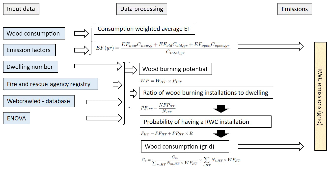
The MetVed model is set up with several routines for the calculation of wood consumption at the at 250 m grid level. A schematic of the model calculations is shown in Fig. 1. Emission factors for three different burning technologies are provided by Seljeskog et al. (2013): old stoves (pre-dates 1998), new stoves (1998) and open fireplaces. Emission factors are combined with aggregated consumption statistics at the county level with the same differentiation. The other main input data sets are the location of fireplaces from the fire and rescue agencies registry, data on dwelling types and available residential heating technology obtained from the largest real estate advertisement portal in Norway, and energy consumption from the Norwegian Energy Labelling System (ENOVA). The model additionally uses outdoor temperature together with a diurnal and weekly variation of woodfuel consumption in Norway to establish the time dependence of emissions. As with most emission models, the accuracy and level of detail depends on the available input data. For MetVed, the model output resolution is determined by the resolution of the input dwelling information (i.e. 250 m).
As the above data sets constitute the basis for the analysis of RWC in Norwegian households we provide a detailed description of each data set in this section. The utilisation of high-resolution data is important for the MetVed model to produce valuable results. The principle behind building an emission model with more bottom-up principles relies heavily on gathered underlying data. Thus, to achieve accurate emissions, new avenues for data gathering is an important field of development.
2.1 Wood consumption
The use of wood for residential heating for the years from 2005 to 2016 is provided based on the responses to the Statistics Norway's Travel and Holiday Survey. Data on wood consumption are collected and officially reported by Statistics Norway at the county level. The survey gathers data in four quarterly surveys covering the preceding 12 months. The calculated consumption of wood is the average of five consecutive quarterly surveys. The survey contains 25 questions regarding wood burning for residential heating. The sampling pool of the survey is drawn at a nationwide level and is considered representative for all counties. Wood consumption in each of the three technology classes (open fireplace, stove produced before 1998 and stove produced after 1998) is available for each county, and these data are used in the MetVed model as input because finer resolution is not available.
Reported wood mass (kg) from questionnaires is recalculated to represent dry wood consumption by assuming an 18 % water content. In that way, wood consumption corresponds with emission factors that represent grams of pollutant per kilogram of dried wood. According to Statistics Norway, there are several elements of uncertainty in the wood consumption data, such as the survey sample size and the employed conversion factors (e.g. mass of bags of wood reported as volume). Statistics Norway concluded that the coefficient of variation of the total wood consumption is below 3 % based on an uncertainty study carried out in 2011 (SSB, 2018). The uncertainty is higher at the county level as the values are based on smaller samples. Large-scale production of fuelwood and sales of wood (estimated 70 % of consumption) are nearly exclusively birch, and also untraded wood will contain significant birch. As no other information is available, consumption is assumed to be birch, in accordance with emission factors.
2.2 Emission factors
The Norwegian emission factors are listed in Table 1 and were established by Seljeskog et al. (2013) for three categories: (i) open fireplaces, (ii) stoves produced before 1998 and (iii) stoves produced after 1998. The emissions factors are determined by laboratory experiments following the Norwegian standard for testing enclosed wood heaters and smoke emissions (Norsk Standard 3059, 1994) and are considered as representative of real-world conditions. The particle sampling is carried out in a dilution tunnel in order to mimic the dilution and cooling effects when the smoke exits the chimney. In this way, the particle sampling also accounts for condensed matter. The Norwegian standard requires that the type of wood used is birch, so all emission factors are based on birch wood.
Table 1Emission factors as amount of pollutant per amount of dry wood (Seljeskog et al., 2013).
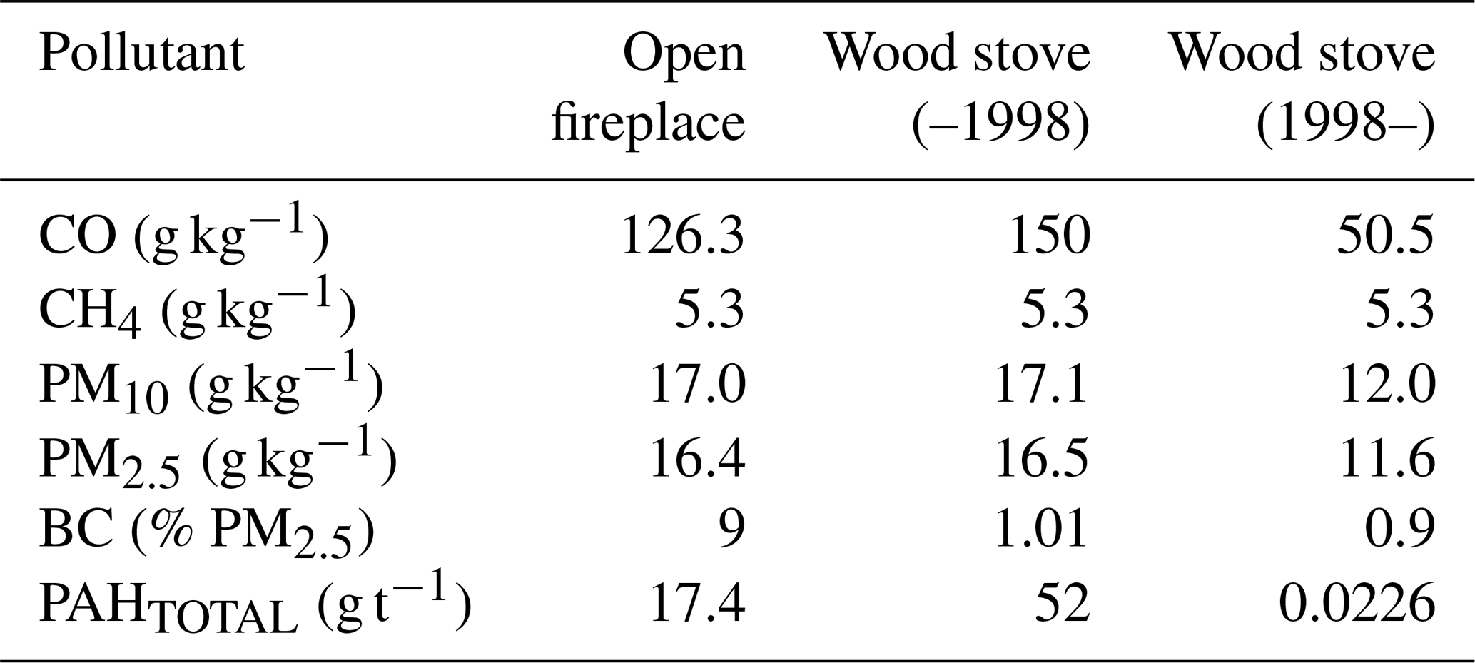
Seljeskog et al. (2013) proposed two sets of emission factors depending on different firing conditions in Norwegian cities and rural areas. The reasoning behind the two emission factors is that users in the countryside fire their stove with low air intake during the night and other users do not (Haakonsen and Kvingedal, 2001). To our knowledge, there is not a solid and updated study that supports this assumption; thus we presume the same firing conditions as in large cities across all of Norway.
2.3 Dwelling number
The data set containing the type and number of dwellings is obtained from Statistics Norway (Bloch, 2018). The data set originates from the state tax agency registry (SERG), and that covers all households in Norway. It can be considered complete and up to date. The gridded version at 250 m of this registry maps the number of dwellings, the number of detached houses, duplexes, townhouses, the number of dwellings in apartment blocks and other dwellings. An example of the dwelling number data set (for the municipality of Stavanger) is shown in Fig. 2. The grid number of total houses (Fig. 2a) has the highest density of dwellings in downtown Stavanger. This is also where apartments (Fig. 2c) have their highest density, while detached houses (Fig. 2b) are much more uniformly spread through out the municipality. This illustrates a typical feature of most urban areas, where a city centre typically consists of mainly apartment blocks, whereas detached houses and duplexes are more prevalent in suburban areas. In Norway in 2017, there were around 2.5 million registered dwellings of which 50 % are detached houses, 9 % duplexes, 12 % townhouses, 24 % apartments and 5 % are classified as others. The spatial distribution of dwelling types differs across region and area. This is especially so for the apartment share, which ranges from 77 % in the Oslo municipality to 0 % in many rural municipalities.
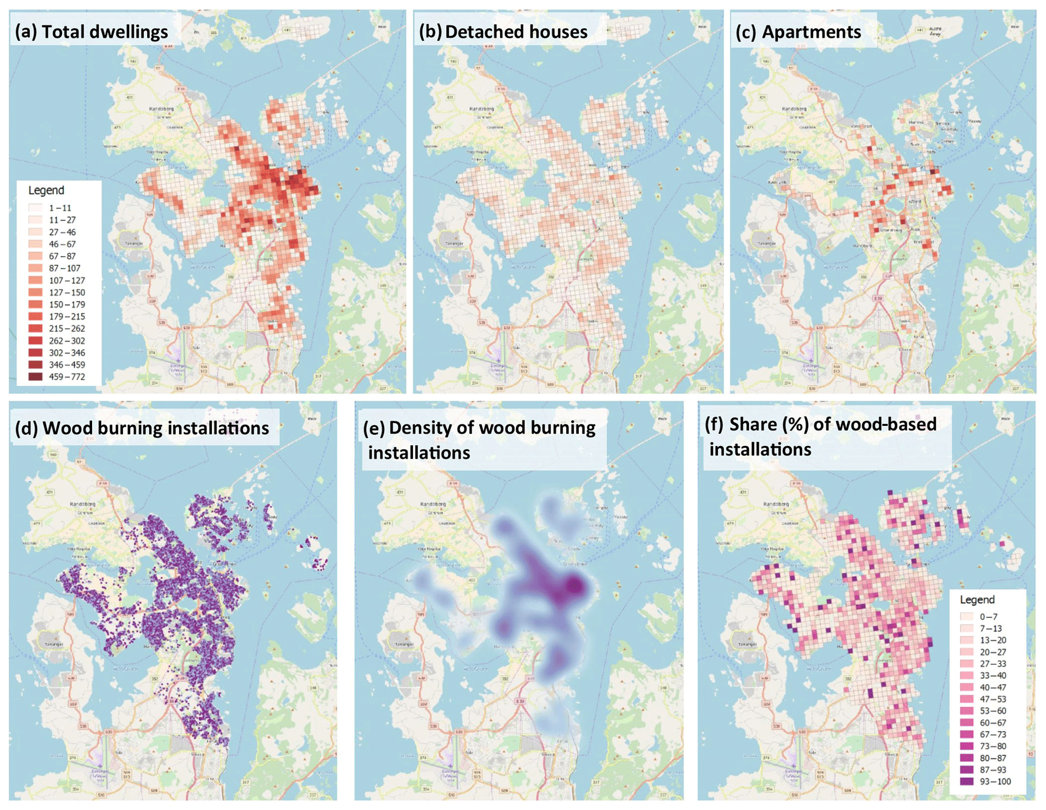
Figure 2Example of part of the input data used in the MetVed model in the Municipality of Stavanger. (a) Total dwelling number at 250 m grid resolution. (b) Number of detached hours. (c) Number of apartments. (d) Individual wood burning installations from the fire and rescue agency. (e) Density of wood burning installations. (f) Share (%) of wood-based installations for residential heating obtained from the web-crawled data set. Background map: © OpenStreetMap contributors 2019. Distributed under a Creative Commons BY-SA License.
2.4 Fire and rescue agencies registry
In Norway, there are 620 fire stations divided among ∼300 fire department agencies. The fire and rescue agencies are responsible for inspecting and assessing all firing installations. These are dominated by residential heating installations, but the database also contains a small number of cooking appliances. The agencies carry out routine inspections as part of fire hazard safety procedures. During these inspections, information such as geographical location and type of installation is collected in a local database by each agency.
In this study, we contacted 270 fire and rescue agencies in Norway to gain access to their data set on firing installations. We successfully obtained the complete information from a total of 101 municipalities, covering almost half (1 million) of Norwegian residencies, including the five largest cities. The data set provides detailed information on all residential addresses inspected, including the geographical location of the pipe, the installation type, technology and model, and whether the technology can be classified as a clean burning technology (i.e. true/false).
The fire and rescue agency registry, if complete, should include all firing installations including those in residential households. There are however a few caveats to these data. Inspections are carried out continuously and over time, and the data obtained generally did not indicate when the inspection was done and some data could be obsolete. There is also a lack of uniform sampling method among the municipalities, and the type of data supplied was different for each fire departments system. For instance, there were 795 different housing types in the total fire agency data, which were filtered to each of the residential types of buildings and others. Classification of the installation ranged from a general description to a complete brand and model type, in all consisting of 890 different descriptions. Each one was placed in one of the three categories of wood burning installation or classified as non-wood based. It also appears that the coverage is not fully complete and must be considered partial even in the municipality where all fire agency data were provided. For example, the fire agency in the Oslo municipality informed us of continual dodging of inspections by house owners for various reasons, which results in an estimated 10 % unregistered firing installations (Oslo Fire Department, personal communication, 2018). As a result, the data are used as a statistical input to the MetVed model. Cross referencing wood consumption and firing installation statistics shows that there is a relatively good agreement with other existing data, and therefore it could also be used directly in the model. Figure 2d shows all the inspected installations in the Stavanger municipality with a density heat map Fig. 2e. The highest density of wood burning installations is obtained in the Stavanger city centre, but there are also other less densely populated areas where fireplace frequency per dwelling is much higher (e.g. Testa, which is north-west of the city centre).
2.5 Web-crawled database
The web-crawled data set is derived from the web-crawling program GoodOvening that scrapes data in a systematic way from a real state advertisement portal satisfying certain search criteria. It structures data obtained for further data analysis (for more details see Lopez-Aparicio et al., 2018). The web-crawled data set is continually updated and consisted of 444 000 geo-positioned data points within Norway at the time the data was extracted for the MetVed model. Along with the geographical location, the web-crawling extracts data on the characteristics of each dwelling such as the type that they belong to (i.e. detached house, townhouse, duplex, apartment, etc.), the size and the type of the available energy system for residential heating (i.e. wood burning installation, district heating, heat pump, etc.). The web-crawling database is aggregated to the 250 m grid resolution and it allows us to establish, with a high level of detail, grids with low or high RWC potential. A zero RWC potential is assigned to those grids with dwellings with no wood-based heating installations. The highest potential would be to those grids with dwellings where a wood-based installation is the sole residential heating source. Between these, the potential is determined as a proportion of wood-based installation to other residential heating technologies.
Figure 2f shows the proportion of wood-based installations for residential heating relative to other listed technologies (e.g. district heating, heat pump, electricity) at 250 m resolution. The city centre shows a low proportion of wood-based technologies (i.e. from 0 % to 30 %) even though the same area shows the highest number of residential dwellings (Fig. 2a) and the highest density of wood-based technologies (Fig. 2b). The highest proportion of wood-based technologies is observed spread out in the areas outside the city centre. We see similar spatial patterns at the grid level for the proportion of wood-based heating technologies in and around other Norwegian cities.
2.6 Database from the Norwegian Energy Labelling System for Dwellings (ENOVA)
The ENOVA energy labelling system was implemented in Norway in July 2010 and is a self-assessment report performed by owners of dwellings and buildings, or qualified experts in the case of new buildings. The ENOVA data set consists of about ∼650 000 entries that include (i) the size of the dwelling, (ii) building type (e.g. apartment, small house, office building), (iii) building year, (iv) energy consumption of the dwelling (kWh), (v) primary and secondary heating installations, (vi) energy consumption per fuel and (vii) geographical information. While individual buildings are listed in the data, the data accessed were used on a municipal and postal code resolution due to data privacy. The information from these data supplements the two preceding data sets and also provides a relation between energy consumption for total heating, RWC and building size/type. Wood consumption input statistics to MetVed were used on the county level to correspond with wood consumption data.
2.7 Outdoor temperature
Outdoor temperature is an important controlling factor for RWC because the main purpose of most RWC is the heating supply. The MetVed model uses observed temperatures as input meteorological data. Observed daily mean temperatures were obtained for the years from 2005 to 2016 for 57 official Norwegian temperature measurement stations through the eKlima database (eKlima, 2018) to form the basis for time variation of emissions for MetVed. For now we have ensured that urban areas have an observation point within them.
2.8 Other data
In addition to geospatial information of Norway, such as municipal and county administrative borders, we have ancillary data responses to questionnaires on wood consumption in Akershus/Oslo and Sarpsborg/Fredrikstad (Lopez-Aparicio et al., 2017b). Together with all of the individual answers of respondents to the questionnaires of the Statistics Norway Holiday Survey (where wood consumption is reported), they form the basis of establishing assumptions on variability between primary and supplementary wood heating habits.
To assess emissions, dispersion modelling has been used and the results have been compared with observations. To do this, measurement data of PM2.5 were taken from the Norwegian air quality network monitoring stations that report to the European air quality database (https://www.eea.europa.eu, last access: 14 June 2019). PM is measured by applying methods equivalent to the reference method (i.e. TEOM 1400A and Grimm-EDM180) that continuously monitor and log with a time resolution of 1 h. Measurements of BC in Oslo were obtained at two roadside monitoring stations in the winters 2014/2015 and 2015/2016. The measurements were performed with an Aethalometer (Magee Scientific) that measured aerosol light absorption at seven specific wavelengths at 1 min resolution (Hak, 2017). The results at the specific wavelengths are used to determine the contribution from traffic and wood burning to BC concentration based on the model established by Sandradewi et al. (2008). Benzo(a)pyrene (BaP) measurements were taken from the Norwegian monitoring network through active air sampling. The monthly B(a)P values are derived from the analysis of particle filters, which are collected with a 3 d frequency. The identification and quantification of B(a)P is carried out by GC/LRMS.
For the MetVed model MatLab was chosen since there is a wide variety in the type form and file format of the input data, and it allows for easy reading, visualisation and inspection of data flows in the model. The MetVed model contains different routines to estimate emissions at the 250 m grid. In order to calculate emissions, MetVed first calculate gridded wood consumption and emission factors. Spatial and temporal distribution of emissions further requires information on location, type and activity of wood burning installations. These are all derived from the input data, which have different scales and resolutions (e.g. county, municipality, grid, point). MetVed calculations take into account the physical properties of households and their heating systems, but they do not account for most human behavioural differences. The main calculation of MetVed is to pre-process the input data to arrive at gridded emissions, calculated as
where E(c,yr) is emissions (g yr−1) in a grid, c, for the year, yr, and C and EF are the wood consumption (kg) and emission factor (g kg−1), respectively. Though several calculation methods are available in MetVed, the main method to calculate grid EFs and consumption is based on consumption per technology at the county scale. The initial step is thus to calculate a consumption-weighted average EF for the year of interest, yr:
where EFold, EFnew and EFopen refer to the emission factors for old stoves, new stoves and open fireplaces, respectively (Table 1), and similarly Cnew,yr, Cold,yr and Copen,yr refer to the consumption in the different technology classes.
To distribute consumption to each grid, MetVed calculates a wood burning potential (WP) in a hierarchical fashion up from dwelling to grid to municipal level and finally up to county, to match the consumption input data resolution. The WP is calculated to distribute in a consistent way the available consumption at the county level, and this establishes the share of total consumption assigned to each grid. The WP is dependent on statistical and physical properties of each residence (e.g. the type and the size), and it has two components:
a consumption weight (WHT) and a frequency of wood-based installation for residential heating (PHT), calculated per dwelling type (HT) in each county. PHT is calculated based on the fraction of dwellings of each type in each county that have listed wood burning installations in the web-crawled data set. For the consumption weight WHT, a linear dependence between energy consumption and dwelling size is applied for each HT and is specific to each county. The linear dependency is established from the ENOVA data set, and the dwelling size applied is the HT average size determined from the web-crawled data set per county.
Survey data on wood consumption, however, indicate very skewed consumption statistics that are not explained by total heating demand of a dwelling. According to the surveys, a few high-intensity users burn up to 30–50 times the average amount of wood consumed, which can amount to more than 10 % of the wood consumed in a given county. This differential usage introduces uncertainty and it will also affect consumption. In broad terms we can distribute the usage rate into three categories: (i) inactive (existing installations not in use), (ii) secondary usage (used as supplementary heating), and (iii) primary heating source. At the moment, there is no way to establish exactly which of the listed installations are in disuse. Therefore, we only consider two categories, i.e. installations for secondary usage and as primary heating source. As an example, the Bergen fire department estimated that roughly 15 % of the wood burning installations are inactive, 70 % are sporadically used for social or secondary heating, and the remaining 15 % are primary heating sources. To detail out further the activity level of fireplaces, further data could be collected. In some municipalities, amount of residue material from chimneys swept is kept record of and graded on a scale from 1 to 9 (clean to dirty). These and similar data (if collected) could be used directly to estimate the activity in each chimney but would need a proper framework. Also the consumption questionnaire presently asks respondents first if they have a wood firing installation and then if it is in use, so this also supports finding the average share of inactive fireplaces.
These usage shares will have geographical variations because climate, wood availability and prices of heating vary across the country. It is therefore necessary to improve the information on installation usage. This is done by the analysis of the web-crawling data set (Lopez-Aparicio et al., 2018). This data set provides good statistics on the relative occurrence of both wood burning installations and other heating technologies at high geographical resolution. When it is established that other heating technologies are available (e.g. district heating, heat pump), wood burning installations are assumed to be used as a secondary heating source.
The difference in wood consumption between a RWC installation that is used as a primary heating source and another that is used as a secondary source has been established through the ancillary data in questionnaires (Lopez-Aparicio et al., 2017b). We define the ratio (R) between wood consumption for households with primary (h1) and secondary (h2) RWC heating as . To represent h1, we used the 15th percentile of consumption and for h2 the average wood consumption to get a conservative estimate of R of 4. In the questionnaire data, RWC as primary heating source occurs only in detached houses, and therefore this is only applied to this type of dwellings, where 10 % of detached houses are assumed to use wood as their primary heating source.
We establish the ratio of wood burning installations to dwellings as
where NHT is the number of dwellings of a specific type and NFPHT is the number of installations per HT. The ratio predicted by web-crawling and rescue and fire agencies data sets predicts roughly 1.7 million installations, while in an existing national survey predicts about 1.9 million houses with wood-based installations (Norstat 2016 survey, Norsk Varme, personal communication, 2018). Therefore, an adjustment was done to the detached houses to assign enough total installations to residences based on web-crawling that gave about 10 % fewer total installations in residential buildings than reported. The probability of having an installation for RWC (PHT) is then calculated:
where PP is the fraction of primary heating for each type of dwelling (HT). Finally, the consumption in each grid is calculated by distributing the municipal consumption Cm to each grid depending on the number of dwellings of each type (NHT) at the grid, c, and their associated WPHT:
where the Cm is calculated in the same way as Cc in Eq. (6) based on wood consumption at the county. For each year, emissions (E(c,yr)) are finally calculated at the grid by multiplying Eqs. (6) and (2) at the grid.
Time variation
From an annual baseline consumption, MetVed estimates the hourly distribution of wood usage through a calendar year. The time variation of RWC activity is defined to be dependent on the heating demand defined by the outdoor temperature. Therefore the heating degree day (HDD) concept is used (Quayle and Diaz, 1980). MetVed looks up the geographically nearest meteorological station to obtain the outdoor temperature data set. Thereafter the HDD is calculated as
where T is the outdoor daily average temperature in degree Celsius. Regarding TThreshold, we follow Stohl et al. (2013) and use 15 ∘C (HDD15). Hourly resolution is obtained by coupling the daily consumption to the diurnal heating cycle in Norway. The time of day when RWC occurs is obtained by a survey covering dwellings that provides information regarding the use of the RWC installations both during the day and week (Aasestad, 2010). The obtained weekly and hourly activity shows a strong diurnal cycle, where RWC is higher after 17:00 CET. Hourly consumption is obtained by multiplying the daily HDD derived consumption with the hourly average reported activity, which is also weekday dependent. There is higher activity during weekends than weekdays (Haakonsen and Kvingedal, 2001). The consumption differences between weekdays and weekends are smaller than what is suggested by Finstad et al. (2004) and Krecl et al. (2008). However, the diurnal pattern of concentrations they found for RWC is similar to the emissions profile derived based on the activity data, which assumes an emission profile that takes into account emissions of the later stages of the firing cycle (e.g. Heringa et al., 2012; Sciare et al., 2013). Fixed public holidays and Easter are treated as weekends.
4.1 Time evolution of wood consumption in Norway
The primary model output from MetVed is gridded emissions for Norway in the period of 2005–2016. Figure 3 shows the spatial distributions of emissions from RWC obtained with MetVed at a 250 m grid resolution in southern Norway and seven domains selected for the evaluation of urban emissions. The distribution of RWC emissions on the 250 m grid is concentrated where there are residential buildings. This is in cities, valleys and along the coast, and consequently they cover a small proportion of the surface area in Norway. Each grid cell has emissions relative to their proportion of the wood burning determined by the number and type of dwellings and available residential heating technology within it. In the urban domains, the lowest emissions (i.e. in the range 0–0.14 t yr−1 per grid) are obtained in the outskirts of the urban areas (blue grids in Fig. 3), whereas the highest emissions (i.e. 0.30–1.50 t yr−1 per grid) are centred in the urban areas. The internal distribution within each urban domain varies among the cities, as it depends on the distribution characteristics of apartments and houses, as well as the availability of non-wood-based residential heating technologies.
.
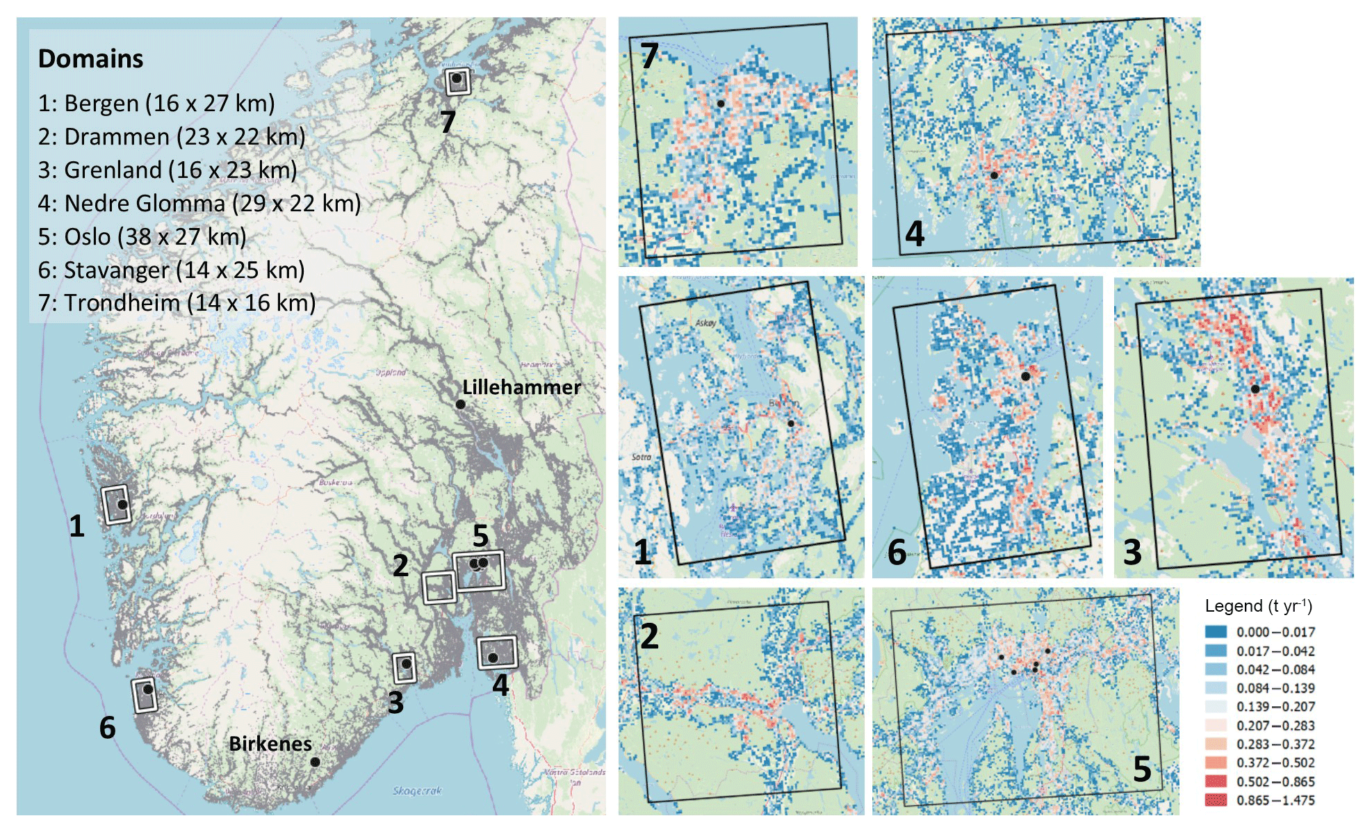
Figure 3MetVed emissions (t yr−1) in 2015 in the south of Norway and in seven urban domains at a 250 m grid. The squares in the map of the south of Norway represent the zoomed in domains on the right, labelled from 1 to 7 (named on the left panel), which are used for the assessment of urban emissions and dispersion modelling. The black circles represent the location of the air quality monitoring stations in Figs. 7, 8 and 9. Background map: © OpenStreetMap contributors 2019. Distributed under a Creative Commons BY-SA License.
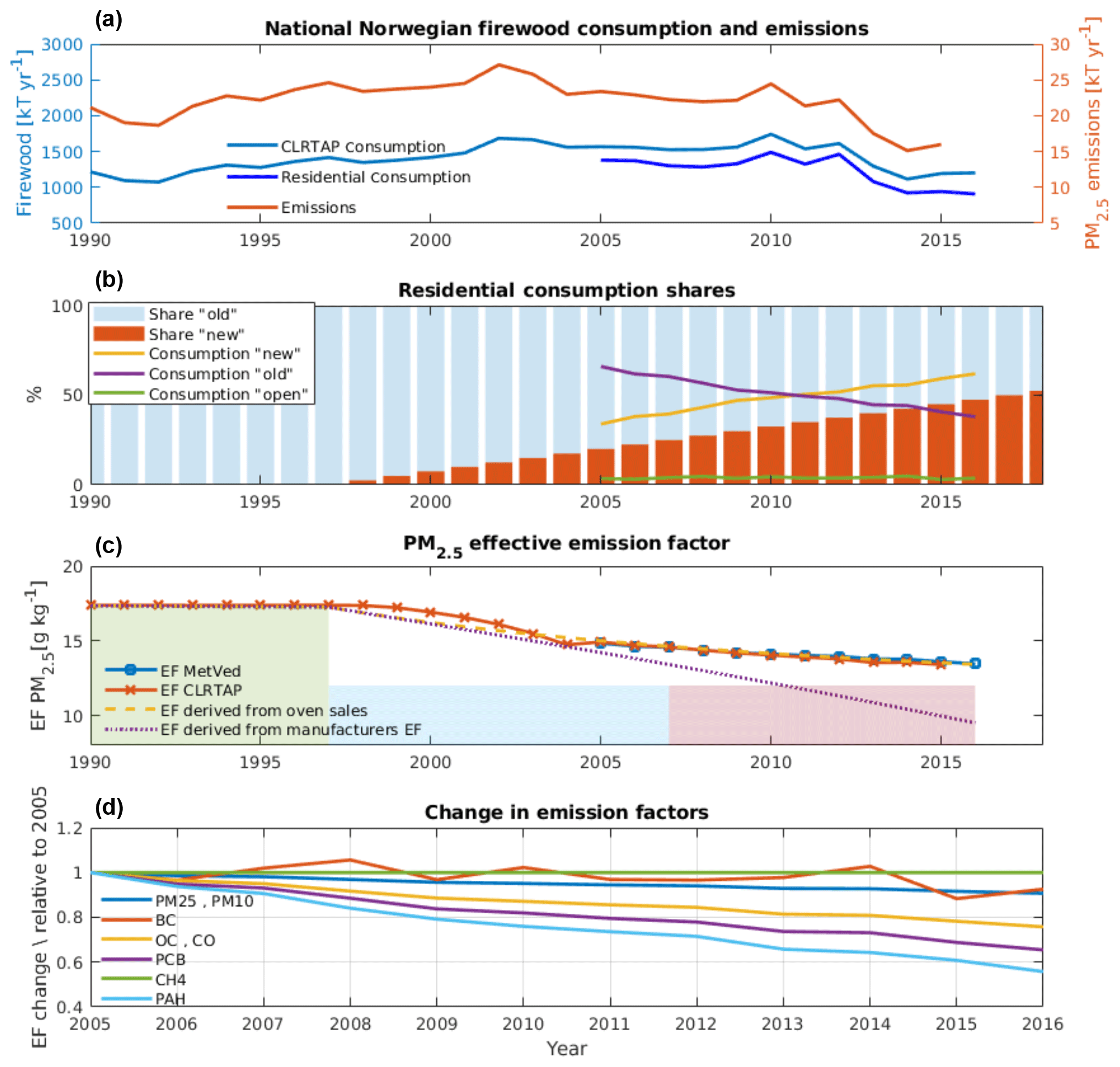
Figure 4(a) Historical evolution of the officially reported consumption of firewood and emissions of PM2.5 since 1990. (b) Consumption per technology class for new, old and open in yellow, blue and green, respectively. Red bars show the stock of new ovens assuming a constant sale over time. (c) The coloured bars show the EF of ovens sold in a given year. EF MetVed (blue) is the emission factor used in the MetVed model. EF CLRTAP is derived from officially reported emission and consumption numbers. The yellow dashed line shows the emission factor one would get from the assumed oven sales (red bars in panel a) and equal consumption in all ovens. The deviating dotted dark blue line shows the derived annual emission factor when manufacturer information on emission factors is used for each year. (d) Annual average emission factors for each year of each component in the MetVed emissions, based on consumption statistics.
Total annual MetVed emissions are closely linked to the total emissions in Norway reported to CLRTAP (Fig. 4a) as both are estimated using the same wood consumption data and emission factors. MetVed wood consumption is only for residential heating, and the difference with emissions reported to CLRTAP is that the latter includes consumption in cabins. The peak year of wood consumption is 2010, coinciding with an especially cold winter across Norway. Since 2010, consumption has gone down every year except in 2012. Before 2005, there was a general decline in reported emissions. This is mainly associated with a reduction in wood consumption and an increase in the share of newer technology ovens. From 2005 until 2016, consumption in open fireplaces is relatively constant, varying between 3 % and 5 %, whereas the share of consumption in new stoves has nearly doubled, from 34 % in 2005 to 62 % in 2016 Fig. 4b).
4.2 Effects of technological advances
In 1998, regulations were put into place to reduce emission for newly sold stoves, which should not emit more than 12 g kg−1 of PM2.5. The bars in Fig. 4c show the assumed average EF of stoves sold in that year. Assuming ovens have equal usage, the share in a given year predicted by an exchange of stoves by sales is shown as a dashed yellow line. This EF fits very well with the derived emission factor for PM2.5 from both MetVed and from the CLRTAP emissions since 2005. Similarly as for PM2.5, all other compounds (Fig. 4d) except CH4 show a general decline in EFs since 2005. This decline in EFs is the main driver for the decreasing trend in emissions in Norway, as an increasing fraction of wood is consumed in new stoves. BC is the only EF that does not decrease uniformly. The reason is that the EF for open fireplaces is an order of magnitude higher than those for stoves, and the slight variability in the consumption estimates in open fireplaces drives the change.
The MetVed input data were analysed to evaluate both the share of stoves and their use. In the fire and rescue agency data, roughly 70 % indicate the age of the installation, of which only 34 % of residential stoves are noted to be newer than 1998. A recent survey carried out in Norway in 2016 shows around 64 % of the wood burning installations in 2016 are new stoves (Norstat 2016 survey, Norsk Varme, personal communication, 2018). Sales estimates based on this survey indicate that the transfer to cleaner technologies therefore will go on for the next several decades. Similarly, the increased efficiency of newer ovens from an estimated 50 % to 75 % for new ovens (Seljeskog et al., 2013) will act to reduce consumption. Thus, based on this, future emissions are expected to go down further. The red bars in Fig. 4b show an assumed share of existing stove technology assuming annual sales of new ovens to the residential sector of 67 500 units per year. This sale is derived from a fit to emission factors and will be influenced by consumption differences. Based on the Norstat 2016 survey, annual sales are close to 40 000 installations per year (Norsk Varme, personal communication, 2018). This difference indicates that there are large consumption differences and that on average a new installation may involve a higher consumption of fuelwood. Therefore, what the real effect of exchanging an old for a new installation will have on the overall consumption, and therefore on emissions, is still uncertain.
It is worth noting that the two stove technologies new and old are comprised of an assembly of stoves. Producers of stoves today claim to have significantly reduced PM2.5 emissions even further since 1998, to about 2 g kg−1 in 2016 (Norsk Varme, personal communication, 2018). Both Norwegian emissions reported to CLRTAP and MetVed assume constant EF for the new oven assembly. The dotted lines in Fig. 4c show the EF with a continuing reduction down to 2 g kg−1 in 2016, both for ovens sold in that year (light blue) and for the share of stoves in that year (green). Were EF based on this it would act to significantly reduce 2016 PM2.5 EF from 13.5 to 7.4 g kg−1 and thus nearly halving emissions.
4.3 Temperature dependence of wood consumption
Consumption of fuelwood follows the change in demand for heating energy. In Fig. 5a the total annual number for HDD15 at observation sites (57 meteorological stations) across the simulation domains in Norway is weighted by the total number of dwellings in the domain covered by each station. The MetVed annual consumption is from the CLRTAP (Fig. 4a), which is derived independently from the temperature. The linear fit to the period 2005 to 2016 indicates that consumption is reduced by ∼6 % per year, whereas a slight increase in HDD demand is observed over the same period (Fig. 7c). Residuals from both trends show that the temperature can explain about 63 % of the variance in consumption (r=0.79 Fig. 5b). HDD would therefore provide a good indicator for present and future annual consumption variations, but long-term trends depending on the physical properties of residences must also be considered. It is also important to note that the trend of decreasing consumption between 2005 and 2016 is not due to increasing average winter temperatures.
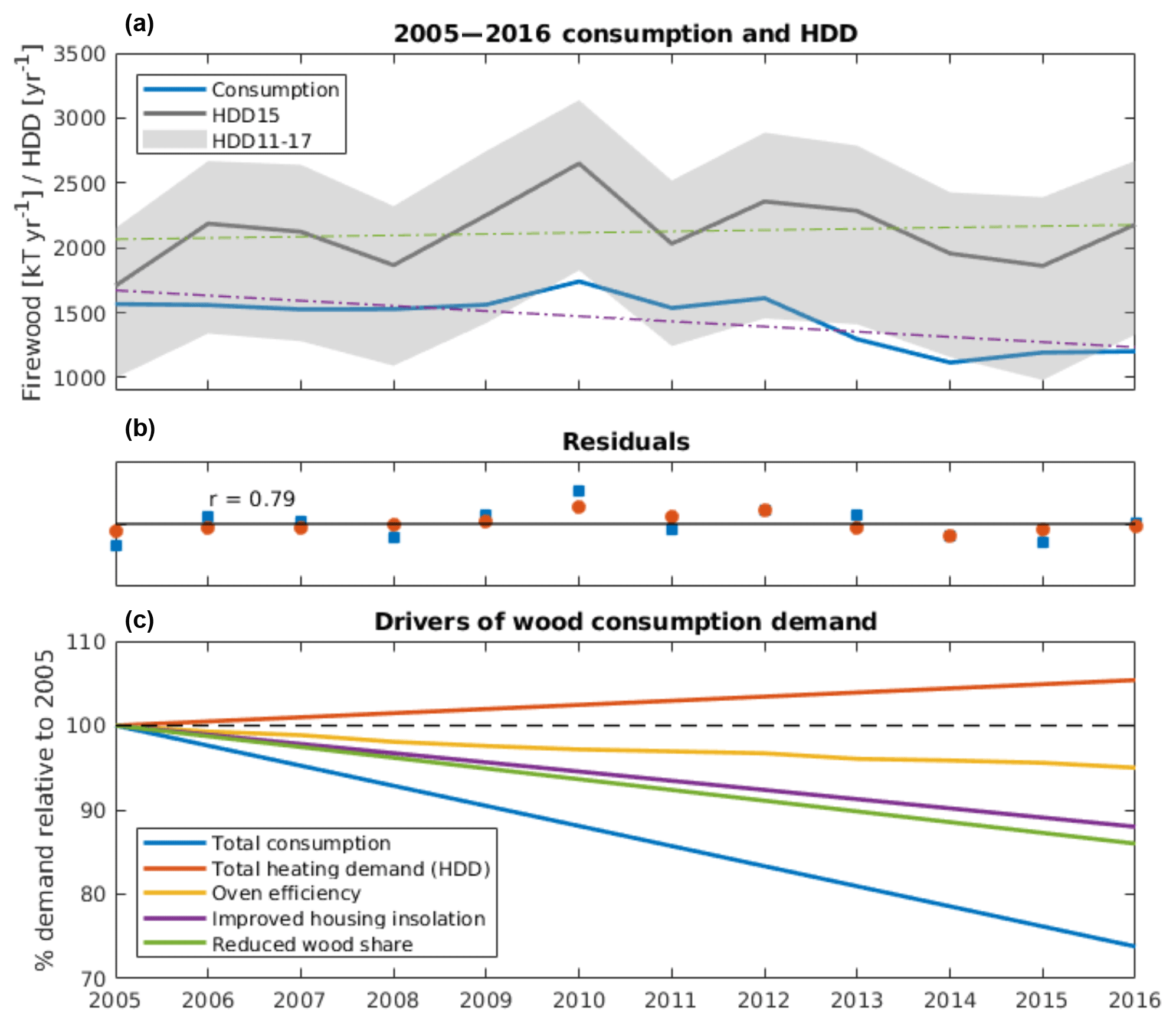
Figure 5(a) The HDD in the simulation domains in Fig. 3 weighted by the population in each domain along with the annually reported consumption 2005–2016. The dashed line is the linear trend. (b) Normalised residuals to linear trends 2005–2016. (c) The blue line show the linear trend in consumption. Explanatory variables for this change (2005–2016) are changes in heating demand (HDD; in red), the efficiency of wood ovens (assumed 75 % for new, 50 % for old and 15 % for open; in yellow), the reduced energy required to heat buildings due to improved insulation (purple), and the decreasing share of total domestic energy consumption that comes from wood (green).
In the MetVed model, the concept of HDD is only used to distribute wood consumption within a year, and only to days with a heating demand. The model determines the total number of HDDs in a year over which the consumption is distributed. The choice of a threshold HDD, i.e. the coldest temperature where no heating is required, only influences the temperature sensitivity of consumption within a year. A lower HDD threshold would therefore only lead to higher emissions in winter and less during spring and autumn. In the cold year 2010, consumption increased by 25 %, and the number of HDDs with threshold 20∘ (HDD20) increased by 23 % relative to the 2005–2016 mean. In contrast, HDD15, HDD10 and HDD5 showed an increase of 36 %, 65 %, 135 %, respectively. Thus a lower threshold temperature will thus increase temperature sensitivity of emissions. From the residual consumption and HDD15 in Fig. 5b we derived the relation for the period 2005–2016:
where ΔC is the change in consumption and ΔHDD15 the change in the HDD15, both unitless. The relation between the outdoor average temperature and consumption is 0.32 kg dwelling−1 HDD.
As other factors also influence wood consumption, household energy consumption per square metre has been examined from the output of the Norwegian energy balance model (https://www.ssb.no/energi-og-industri/statistikker/husenergi/hvert-3-aar/2014-07-14, last access: 18 December 2018) and shown in Fig. 5c. An increase in the number of energy-efficient houses and a lower wood energy share reduce the annual wood energy demand (both by ∼1 % per year in Fig. 5c). Seljeskog et al. (2013) report an energy efficiency of 15 %, 50 % and 75 % for open fireplaces, old stoves and new stoves, respectively, which are also used in the Norwegian energy balance model. Consumption per technology in 2012 gives a 61 % average stove efficiency, at a constant energy output. The effect of newer, more-efficient installations has influenced the decrease in consumption by 0.5 % per year (“oven efficiency” in Fig. 5c).
In 2012, the average reported dwellings in Norway received 16 % of their energy, about 3200 kWh, from wood. This is significantly higher than the average energy share suggested by the MetVed input data from ENOVA, where the annual average energy from wood is 960 kWh, although only 3 % reported using wood for heating. The reason for the lower reported wood consumption in the ENOVA data set is not clear but may be related to conscious under-reporting to achieve a better energy certificate by the dwelling owners. Birch wood, which is the most common fuelwood in Norway, has a dry (0 % moisture) energy content of 4.395 kWh kg−1 (Raymer, 2006). To achieve the stated energy, an average Norwegian household would then in 2012 have to burn 1195 kg of dry birch wood. The same conversion of the ENOVA-reported consumption gives 7.2 kg of dry wood for an average Norwegian household. Based on the official wood consumption data, the total residential consumption in 2012 was 1460 kt, which equates to 589 kg of wood consumption per dwelling (800 kg per dwelling with a wood-based installation). Due to large differences in the input data, the housing type and size and energy dependencies calculated within MetVed are only based on the ENOVA-reported total energy consumption.
4.4 PM2.5 emissions at the urban scale
The main aim of MetVed was to improve the spatial and temporal distribution of emissions from RWC. Resulting emissions of PM2.5 within each of the urban domains in Fig. 3 from MetVed are shown with four other emission inventories available to do urban modelling in Norway in Fig. 6a. These domains contain the largest cities in Norway and together cover 44 % of Norwegian dwellings. With the exception of Norsk BeregningsVerktøy (NBV) emissions, all urban emission inventories are obtained by downscaling national emissions submitted to the CLRTAP (http://www.ceip.at). Though the year of reference varies between inventories, the magnitude of total national emission is comparable. The difference within these domains is therefore to a large extent determined by the method of spatially distributing the emissions.
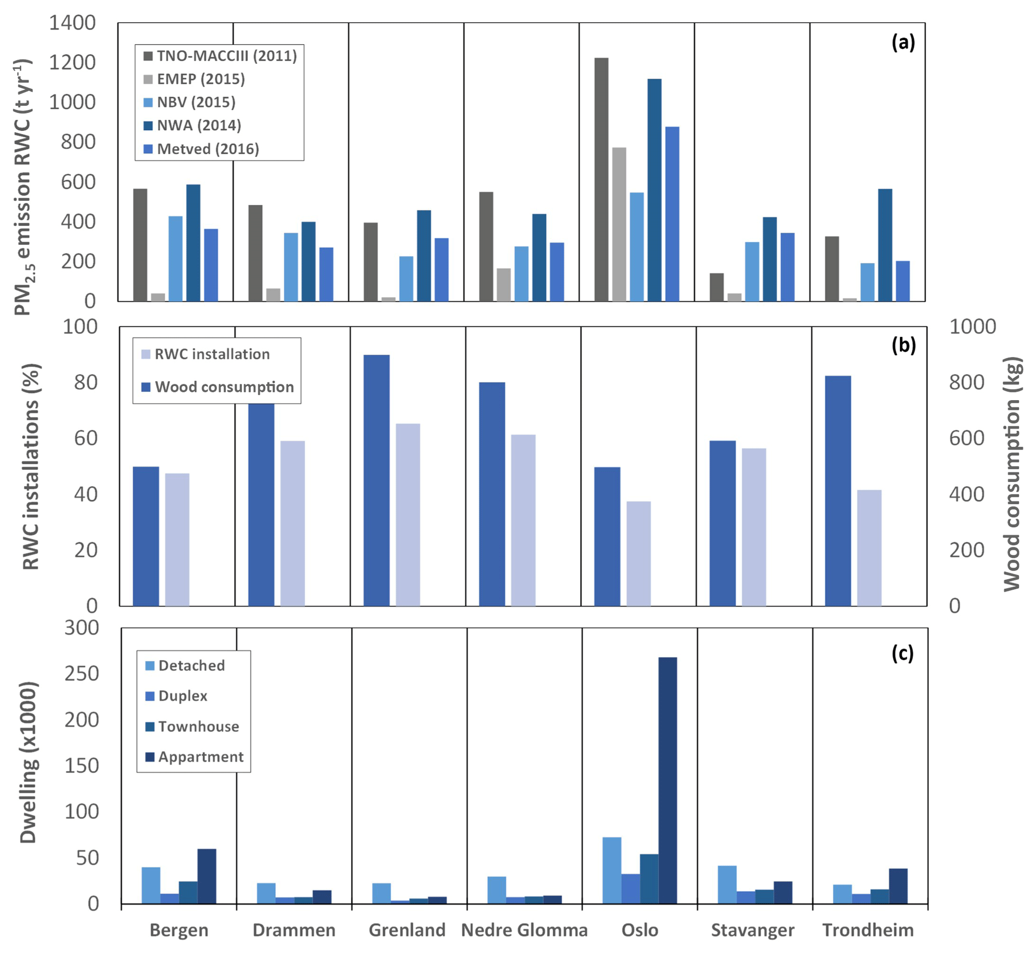
Figure 6(a) Total emissions within domains shown in Fig. 3. (b) The percent of houses with at least one fireplace (left y axis) and the consumption per fireplace for each of the domains (right y axis). (c) The distribution of housing types for each domain.
Total emissions within each domain are computed by first-order conservative remapping emissions for each inventory to the domain (e.g. Jones, 1999). The European Monitoring and Evaluation Programme (EMEP) emissions are distributed on a grid and represent the lowest urban emissions in all domains, except Oslo, having an order of magnitude lower emissions than the remaining domains. To our knowledge, detailed information about the method used to downscale the EMEP emissions is not publicly available, but the data are openly available at https://ceip.at. NEA (2018) states that when the activity data used to estimate emissions are available at a higher geographical resolution than national, they are used to distribute emissions. In Norway, wood consumption is available at the county level; thus we assume that EMEP emissions from RWC are distributed at this level. This is consistent with the visualisation of emissions where the county administrative borders are visible, and emissions are widely distributed in the Norwegian geography, covering also unpopulated areas. The TNO_MACC_III emissions have a resolution of , similar to EMEP, but have much higher emissions within each urban domain than EMEP. TNO_MACC_III uses internal approaches based on population density and a function to describe proximity to wood as their downscaling method (Kuenen et al., 2014).
NWA emissions (NordicWelfAir, http://projects.au.dk/nordicwelfair/, last access: 16 June 2019) are on a 1 km grid and are based on scaling down wood consumption per technology from county level based on dwelling number at 250 m resolution. Different RWC activity is assumed for apartments and houses, and the Norwegian official emission factors (Table 1) is used. Thereafter emissions are re-gridded to a 1 km resolution. NBV emissions, also on a 1 km grid, result from downscaling wood consumption per technology by dwelling number at the district level resolution also using the Norwegian official emission factors (Tarrasón et al., 2017). The domain of Oslo in NBV is an exception. In this case emissions are reported in Lopez-Aparicio et al. (2017b). In NBV, a multiplication scaling factor was derived for each urban domain individually based on the ratio of concentration levels obtained by atmospheric dispersion modelling to observed PM2.5 levels. These factors vary from 0.42 to 0.27, i.e, dividing the total emissions in these areas by a factor of 2.3–3.7. For the MetVed emission inventory, the total emissions within the area are dependent on all the input parameters detailed in Sect. 3.
The total emissions within each domain is for all inventories (with the exception of EMEP) closely related to the number of houses within each domain (Fig. 6b), either directly or indirectly through population. Note that the sizes of the domains vary somewhat and all have different total area (Fig. 3), but they all cover a city and their area of influence. The dependency on dwelling or population density differs among the methods, and thus emissions at the urban scale vary accordingly. TNO_MACC_III results in the highest emissions at the urban scale followed by NWA emissions, but EMEP results in very low emissions at the same scale, as the downscaling approach distributes and diffuses emissions at the county level. In the MetVed model, the emissions are determined by the physical properties of the houses and their installed heating technologies within each domain (also done on the 250 m grid). In our study, we consider NBV emissions as a tuned emission data set, as they have been obtained by comparing results from dispersion modelling and observations, and then scaling emissions. The correction factors vary among the domains and therefore the methodology lacks consistency. However, MetVed emissions are produced at high resolution at the national level following a consistent methodology and relationships between variables that influence emissions. In addition, MetVed emissions at national levels equal the official emissions reported to the CLRTAP which gives it consistency as a national emission inventory. The results from the MetVed model at the urban scale are consistent with NBV for most of the domains. MetVed emissions within the urban domains have, for most of the domains, lower emissions than those derived as a result of downscaling approaches based on population (TNO_MACC_III) or dwelling density (NWA). The MetVed emissions are the most similar to the locally corrected NBV emissions. This lowering of urban emissions in MetVed relative to emissions from the downscaling approach is the result of taking into account the share of wood-based technologies from the web-crawled input data. In that way, we account for lower wood consumption when heating technologies other than wood-based technologies are available (Plejdrup et al., 2016).
There are a number of dependencies in the consumption and wood installation statistics for these domains (Fig. 6b). For instance Trondheim, which has the fourth highest population, is located in the county with the second highest consumption per dwelling, and it has the second highest consumption per wood installation (after Grenland) of any domain. For NBV emissions, this leads to an observation-based emission correction of 0.33. In MetVed, Trondheim's high share of apartments (Fig. 6c) and low frequency of fireplaces (Fig. 6b) gives the lowest emissions for all of the MetVed domains, which shows that these properties act well to explain the reduced consumption. Dwelling size is an important factor for calculating consumption in MetVed, and it plays a significant role because apartments in the Trondheim city centre are generally small. The Oslo domain similarly has low emissions per dwelling, but in this case it is also driven by a low consumption per wood burning installation.
An increased prevalence of wood installations is positively correlated (R2=0.44) with higher consumption within the domains (Fig. 6c). This is a result of the MetVed calculations, where the combination of regional consumption statistics and the prevalence of wood installations is found by the web-crawled statistics. This acts to support assumptions made in previous studies, e.g. proximity to wood and rural consumption being higher than urban consumption, but is in MetVed represented in dwellings' heating installations and their usage rate. Additionally, MetVed considers the dwelling size which further increases a rural amplification of firewood use, as rural properties are on average larger.
Atmospheric dispersion modelling was carried out for PM2.5 for the year 2015 with supplementary runs for BC and additional investigation of benzo[a]pyrene (B(a)P) concentrations at sites where measurements were available. In the selected Norwegian areas, B(a)P measurements may be considered a tracer for wood burning activity. The black carbon from biomass burning (BCBB) measurements available enables the comparison with RWC BC concentrations. The evaluation of BC and B(a)P adds to the comparisons to PM2.5 measurements, which have the added uncertainty of other sources. The combined outcomes from these evaluations will add to the understanding of the uncertainties associated with emissions from RWC and their contribution to air pollution levels in urban areas.
RWC emissions from MetVed for 2015 were used as input in the air quality model EPISODE (Hamer et al., 2019), an offline Eulerian dispersion model frequently applied to assess air quality in Norwegian cities. EPISODE is driven by meteorology from the AROME model (Seity et al., 2011) at 1 km resolution. PM2.5 boundary conditions come from CAMS daily forecast re-gridded to the same vertical and horizontal grid as the EPISODE model (Marécal et al., 2015). In EPISODE, PM2.5 is treated as an inert particle, subject only to removal by transport, which limits the size of the modelling domains. Furthermore, EPISODE requires emissions on the same scale as the meteorology; therefore MetVed emissions were regridded to the meteorological field grid (1 km) within each domain.
5.1 Particulate matter (PM2.5)
The dispersion modelling in the seven domains of PM2.5 was compared to available measurements of total PM2.5 concentration. Comparisons must therefore include all anthropogenic emissions in the urban areas. The additional emission inventories include, along with RWC, emissions by shipping, off-road machinery, traffic exhaust and suspension of road dust. Urban emissions are estimated based on high-resolution input data that thereafter are aggregated to a 1 km grid and combined with time variation functions to result in emissions at 1 h km2 resolution (for more details see Tarrasón et al., 2017; Lopez-Aparicio and Vo Thanh, 2017). Non-exhaust emissions associated with tyre and road wearing processes and the suspension of road dust were modelled by the vehicle abrasion and suspension model NORTRIP (Denby et al., 2013). Emission domains and the year of reference (2015) were chosen to be able to compare with modelled concentrations obtained based on NBV emissions (Tarrasón et al., 2017). Similarly, measurement stations were selected to coincide with the existing model concentrations and assess a potential improvement when comparing with previous estimates.
With few exceptions, the air quality stations are classified as traffic stations and are operated by the road authorities. Few measurements are therefore ideally located with regards to a detailed evaluation of the spatial distribution of emissions from RWC within each domain. The main difference of the spatial distribution provided by MetVed and that by other methods not differentiating housing types (and size) and available residential heating technologies can best be seen through comparison between stations situated between different types of buildings. In Oslo for instance, only one monitoring station (Smestad) could be qualified as located in an area dominated by detached houses, together with similarly located monitoring stations Vaaland in Stavanger and Lensmannsdalen in Grenland. The remaining stations are in close proximity to apartments or a diversity of dwelling types, along with roads with large emissions. Together with the contributed uncertainty from other sources the differentiation on housing types is therefore hard to evaluate, and so the main focus is on evaluating total emissions within each domain.
Table 2The 2015 hourly concentrations fit to observations for EPISODE simulations of PM2.5 for each of the stations. The hourly R is the Pearson correlation coefficient and bias is calculated as model minus observation.
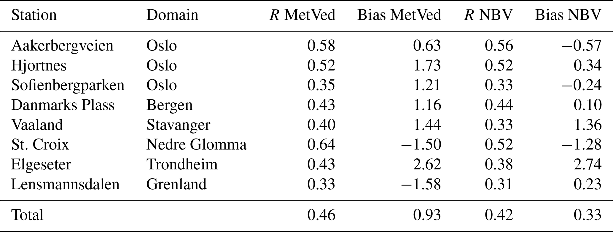
Hourly correlation coefficients and biases are shown in Table 2. Compared to NBV emissions, which were calibrated with a weekly correction factor, the MetVed temporal emission profile generally improves correlation. The bias is not improved, because the MetVed emissions are generally higher, and so the overestimation by the model is increased. The Oslo comparison shows a strong overestimation, and a possible reason is that the MetVed approach has a limited effect in Oslo, as it is in itself a county, and so total consumption and emissions are direct results of the input wood consumption. In the Trondheim domain, the NBV emissions results from applying a factor of 0.33 to the dwelling density derived emissions (Tarrasón et al., 2017), and MetVed produces similar results to NBV at the Elgeseter monitoring station. The consideration of dwelling type and size and the fireplace information accounted for in MetVed account similarly for lower emissions and concentrations in urban areas as the local scalings applied individually in NBV.
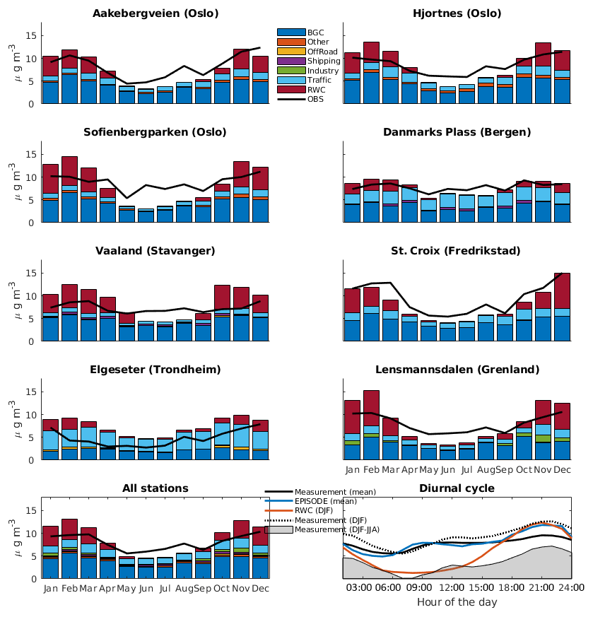
Figure 7Average concentration of PM2.5 averaged at air quality stations and as a total annual average. Bottom right: the annual average diurnal variability concentration as indicated by measurements (black) and the model (blue). The orange line shows the contribution from wood burning and the shaded area is calculated as the measurement hourly average in winter (NDJF) – summer (JJA). The bars show the monthly average concentration by sector and the black line the measurement monthly average.
The annually averaged observed concentration at the sites is 8.0 µg m−3, and using MetVed emissions this is 8.7 µg m−3. Monthly observed concentrations at each station are shown in Fig. 7 as a black line, and the modelled concentrations are shown as bars, coloured by sector. Both model and observations show a pronounced seasonal cycle in PM2.5 concentrations with a winter peak primarily driven by the background concentration and RWC contributions, and the remaining sectors have a similar cycle but contribute less to the PM2.5 seasonality. Model concentrations, including RWC, have a winter to summer (i.e. DJF to JJA) ratio of ∼2, and the measurements have the winter (DJF) to summer (JJA) ratio of 1.45, indicating that the seasonality in model concentration is more than twice as strong. As wood burning for residential heating is an intensive winter activity in Norway, it is hard to envision that there should be no seasonality in RWC, and therefore the uncertainty on the seasonality of other contributing sectors must be considered. Yttri et al. (2011) reported, based on simultaneous measurements in Oslo and a regional background site (Hurdal, 70 km NE of Oslo), similar PM1 values in summer at both sites, 7.6 and 7.7 µg m−3, respectively. However, in winter, PM1 concentrations in Oslo were similar to summer concentrations, i.e. 7.8 µg m−3, but at the regional background site they were 45 % lower than in summer, i.e. 4.3 µg m−3. Source apportionment also indicated that the elevated urban wintertime concentration consisted largely of organic mass from biomass burning. These results indicate a strong urban source rather than influence from regional background levels during winter.
The diurnal evening PM2.5 peak in winter (Fig. 7, bottom right) is also more pronounced in the model than that in the observations. While the difference between the summer and the winter diurnal pattern is also enhanced by meteorological conditions, the absolute difference between winter and summer (i.e. DFJ–JJA grey shape in Fig. 7, bottom right) is much less prominent than the diurnal winter contribution of RWC alone (orange line in Fig. 7, bottom right). The assessment of the diurnal variation also suggests that the total modelled influence of RWC on the air quality station PM2.5 is too strong.
In Oslo, three model simulations were used to assess the sensitivity of surface concentrations to emission altitude. In urban Oslo, the annual average RWC concentration of PM2.5 at 2 m was 4.41 µg m−3 when all RWC emissions were emitted in the surface layer (0–30 m). When apartment emissions were emitted in the second layer, the surface concentration was reduced to 3.76 µg−3, and when smaller buildings emit in the second layer, a further reduction to 3.19 µg−3 was observed. The wintertime diurnal cycle of PM2.5 has a more pronounced peak, and the seasonal cycle of PM2.5 similarly indicates a too-strong seasonal cycle obtained with all emission estimates, when compared to observations, and so the total contribution of RWC to PM2.5 concentrations seems to be overall overestimated. This is supported by the new emission inventory developed by Denier van der Gon et al. (2015) for particulate emissions from RWC. When assessing organic carbon emissions, Denier van der Gon et al. (2015) establish that while emissions in most of Europe are underestimated, in Norway they are overestimated.
5.2 Black carbon
During both winter 2014–2015 and 2015–2016, hourly concentrations of aerosol absorption were measured at two sites in Oslo (Smestad and RV4 Fig. 8). The first period was at Smestad (17 December 2014–18 March 2015) and the second at RV4 (20 November 2015–30 May 2016). The decomposition of the absorbing aerosols includes BC from biomass burning (BCBB), which in Oslo (in winter) should be equivalent to BC from RWC. While both measurements were done in close proximity to larger trunk roads, Smestad is surrounded by a large area of detached houses, while the RV4 sampling site is characterised by apartment buildings and a hospital. Even though the number of dwellings in the area surrounding RV4 is higher with nearly 30 % more residences within 300 m, MetVed emissions in the grid of RV4 are 10 % lower, as the area is characterised by a high share of apartment buildings with low MetVed emissions.

Figure 8(a) The left y axis shows modelled RWC BC (blue) and measured BCBB data at Smestad and RV4 (in red and yellow respectively). The right y axis shows the time series of temperature at Blindern (grey). (b) Aethalometer concentrations of BC from wood burning against temperature measured at two sites in Oslo from winter 2015 to spring 2016 (red symbols) and EPISODE concentrations (RWC BC) in winter and spring for the calendar year of 2015 (blue symbols). (c) The diurnal profile of BCRWC averaged over winter 2015 to spring 2016 as measured by the Aethalometer (blue). The diurnal profile of firing habits as reported by wood consumers in Aasestad (2010) shown in dashed lines for weekdays and weekends (red dashed lines). The dotted lines show the diurnal variability in emission in MetVed.
The modelled year (2015) does not completely overlap with either of the two measurements (Fig. 8a), and therefore model data are shown for the temperature range (T<8 ∘C), which is the temperature range covered by the observations in Fig. 8b. Daily average BCBB concentrations at both sites show a similar dependence on temperature Fig. 8c, though overall lower concentration levels are observed in RV4, which is probably influenced by the measurements continuing further into spring. The difference between the two sites is somewhat smaller in the model. Model concentrations show a similar but weaker temperature dependence, suggesting that daily emissions could increase more than emissions obtained by HDD15.
The modelled diurnal variability in concentration (Fig. 8c) agrees well with BCBB. The diurnal time variation of wood consumption and the subsequent MetVed emissions is in agreement with the BCBB observations. The diurnal weekend emission profile is similar to the observed hourly concentration profile, and the total average model concentration fits (T<8 ∘C) well with the levels of measured BCBB.
5.3 Benzo(a)pyrene
For most of the air quality stations, dispersion model results show an overestimation of winter PM2.5 concentrations, and a similar underestimation of summer concentrations. While PM2.5 has many sources, B(a)P filter measurements offer a way to more directly investigate the RWC contribution.
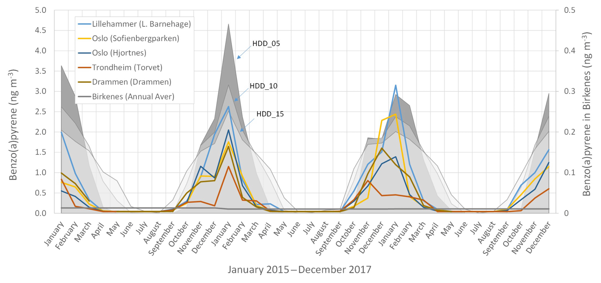
Figure 9Monthly average Benzo(a)pyrene air concentrations at five urban sites in Norway along with the annually averaged concentration on Birkenes, a rural background station in the south of Norway. The shaded areas show the monthly RWC activity predicted by HDD with a temperature threshold of 5, 10 and 15 ∘C.
Figure 9 shows monthly average concentrations between 2015 and 2017 at different urban sites, within the domains in Fig. 3, along with the annual average B(a)P concentration at Birkenes, a regional background air quality observatory. All urban measurement sites show the same B(a)P seasonality with the highest values in January. The most pronounced B(a)P profile is obtained in Lillehammer, followed by Oslo and Drammen, where measurements show similar monthly profiles and concentration levels, and Trondheim, where the lowest B(a)P levels are obtained. The B(a)P annual mean concentration in all urban areas varies from 0.18, 0.30 and 0.20 ng m−3 in Trondheim to 0.56, 0.61 and 0.68 ng m−3 in Lillehammer in 2015, 2016 and 2017, respectively. These levels are below the B(a)P European target value (i.e. 1 ng m−3) but above the reference value established by the World Health Organisation (i.e. 0.12 ng m−3). Unlike in Birkenes, where values represent regional background levels, B(a)P annual mean concentrations are below the WHO reference value, measured at 0.013, 0.010 and 0.011 ng m−3 in 2015, 2016 and 2017, respectively. Figure 9 shows in addition the monthly normalised HDD15, HDD10 and HDD5 obtained for Oslo (grey shades areas) based on outdoor temperatures for the same period. In MetVed, the monthly normalised HDD relates outdoor temperature with activity (i.e. wood consumption). Figure 9 shows the effect that different thresholds (i.e. 5, 10 or 15 ∘C) would have on monthly wood consumption and therefore emissions. A higher temperature threshold will increase activity into spring and autumn, and a lower temperature threshold will limit activity to wintertime. The overall B(a)P best fit to these profiles is obtained using HDD5, suggesting a more intense source during winter than what is obtained with HDD15. This is in agreement with the BC observations, which is the opposite of what is observed based on PM2.5 measurements.
The annual B(a)P average level at each site is indicative of total RWC activity in the area, and the levels are well in agreement with the spatial distribution of emissions in the MetVed model. Lillehammer, with the highest B(a)P levels, is the least densely populated area of those considered here but has high emissions from RWC due to high wood consumption in the region, and the area surrounding the station is made up of mainly detached houses with a high wood burning potential. Trondheim, with the lowest B(a)P levels, is a highly populated urban area located in a county with a high wood consumption. The proxies behind MetVed entail the lowest emissions compared with other urban areas (Fig. 6a) as a result of the high share of apartments with alternative residential heating sources other than wood based, which represent the observed B(a)P differences well.
The uncertainties in emissions from RWC at the urban scale rely on those in the activity (wood consumption), emission factors and spatio-temporal distribution of the emissions. With the development of the MetVed model, our aim was to reduce the uncertainties associated with the spatio-temporal distribution of RWC emissions for their use in air quality modelling at the urban scale. As the spatial distribution alone cannot explain the large uncertainties, a detailed evaluation of the estimations and evolution of wood consumption and emission factors was also performed. The emissions from RWC in Norway show a significant declining trend. This is driven primarily by the increased use of new technologies for RWC along with a general decline in heating demand from wood-based installations through a lower heating demand per square metre and a lower share of total demand being filled from RWC.
MetVed takes into account the physical properties of residences and, based on the frequency, size and type of dwelling and its available heating technologies, estimates a wood burning potential at the grid level. Even though MetVed takes into account most of the variables that affect emissions from RWC, there are still factors not considered which may affect local emissions, e.g. human behaviour, or specific geo-localised information on which installations are unused. Compared with existing emission inventories, MetVed has a higher spatial resolution, which is supported by detailed input data. The unique set of input data, and the established relationships, lead to an improved horizontal and vertical spatial distribution of emissions. One of the main effects of the MetVed approach, when comparing with other methods, is that emissions are displaced from highly populated downtown areas to the urban outskirts. As a result, MetVed gives lower emissions in highly populated areas than those established by downscaling approaches based on population or housing density, and it is moreover in agreement with total local emissions developed by combining results from dispersion modelling and observations. The new approach may have implications when estimating population exposure to pollution levels associated with RWC, as lower population exposure may be expected.
Downscaled emissions derived from annual wood consumption with national emission factors have in the past produced outcomes that did not compare well with observations in Norwegian cities. When comparing with air quality monitoring stations measuring PM2.5, which exist predominantly in urban areas, modelled results have shown a strong tendency to overestimate concentrations. The MetVed model applies several new data sources to the effect of drastically reducing the emissions in urban domains when comparing with direct downscaling methods, and the results are similar to those adjusted by measurement data. The overall correlation is improved even compared to emissions adjusted with observations (NBV emissions), and this highlights the advantages of the MetVed methodology for improving the temporal variability. However, MetVed emissions still overestimate PM2.5 concentrations. The comparison of BCBB indicates, for the same domain where PM2.5 is overestimated, that emissions are on the contrary lower and less temperature dependent than observations should predict. A potential reason for these discrepancies is that the PM2.5 Norwegian emission factor applied could be too high, which would fit well with all the inter-comparisons with observations. This is also supported by the diurnal cycle concentration profile of MetVed emissions, which have a very similar but stronger profile to that predicted by observations of PM2.5 and BCBB, which implies that PM2.5 emissions are somewhat overestimated.
The temporal emission distribution follows the heating degree day (HDD) combined with a diurnal consumption derived from consumer statistics. The applied HDD improves correlation against measurements relative to the emissions adjusted based on observations. However, this gives more intense emissions during winter and a stronger diurnal variability compared with profiles inferred from PM2.5 observations. The Annual average bias is only 0.23 µg m−3 (or 3.83 %), where the winter overestimation is compensated for by the summer underestimation. Across all stations for which simulations were done, the same general temporal pattern is seen. Substantially higher RWC emissions in the summer months or that emissions occur much earlier in the day across all domains are not plausible reasons for the observed discrepancies between winter and summer. Besides, observed BCBB and B(a)P indicate a stronger dependency on temperature, which would produce a stronger seasonality, than predicted by HDD15 used in MetVed. We are confident that the spatial distribution of emissions given by the MetVed model entails lower uncertainties than previous methods based on downscaling approaches using population or dwelling number. Thus, further investigation of the accuracy and representativeness of the activity data (wood consumption) and the official Norwegian emission factors is needed. In addition, the main contributor to the seasonality in PM2.5 is, along with RWC, the background concentration which does not have a diurnal cycle. The evaluation of the PM2.5 seasonality shows the need for improving the time variation of all contributing emitting sectors.
EPISODE RWC PM2.5 surface concentrations in Oslo decreased by 18 % when apartment emissions were shifted from the surface layer (>30 m) to the second model layer (30–60 m). A similar effect at the surface was (further reduction of 14 %) observed for moving all emissions up into the model second layer. This shows the sensitivity to emission altitude when comparing with surface concentrations.
Even though the model is developed for Norway, the principles behind it and the methodology can be applicable in other European countries where similar input data could be made available. Besides, the principles applied in MetVed, which is based on high-resolution data collection, could be expanded to other emitting sectors. To further improve RWC emission inventories, there is a need for more measurements specifically targeting RWC in Norway, as most measurements are limited to PM2.5 at roadside stations in urban areas where the signal-to-noise ratio of RWC is very low. The results and evidence from our study point to even higher emissions from RWC than predicted by observations. As MetVed reduced the uncertainties associated with spatio-temporal distribution of emissions, there is a need to revise the activity data and emission factors used for the official reporting of emissions.
Both MetVed input and output data will be distributed freely upon contact with the corresponding author. Model input data are openly available from their stated source or upon contact with the corresponding author. For underlying ENOVA data, which were obtained under a confidentiality agreement, we refer to ENOVA for distribution. Measurement data can be obtained from the corresponding author or through their source portal.
HG and SLA contributed equally to the text and work within this paper. SLA did all the MetVed EPISODE model simulations. MV contributed to both the writing of the text and method and model development. CH provided the BC measurement data and contributed comments and corrections to the manuscript. AKH provided the B(a)P as well as comments and corrections to the manuscript. DVT did data processing and supplied emissions for other sectors. PH supplied background concentrations and commented on and proofread the manuscript. GSS did all the EPISODE NBV simulations and provided technical assistance with EPISODE and existing emissions.
The authors declare that they have no conflict of interest.
We thank ENOVA for sharing their anonymous data on residence energy consumption, as well as all 90 fire and rescue agencies that supplied data on firing installations.
This research has been supported by the Norwegian Environment Agency project MetVed (grant no. 2017/8676), NFR (grant no. 247884/O70), NordForsk NordicWelfAir Project (grant no. 75007), and NILU Institute Strategic Initiative MASTER (grant no. B118006).
This paper was edited by Jennifer G. Murphy and reviewed by two anonymous referees.
Aasestad, K.: Vedforbruk, fyringsvaner og svevestøv Dokumentasjon og resultater fra undersøkelse i Drammen 2006/2007 Statistics Norway, Oslo, Norway, ISBN 978-82-537-7823-5, 2010. a, b, c
ACAP: Reduction of Black Carbon Emissions from Residential Wood Combustion in the Arctic – Black Carbon Inventory, Abatement Instruments and Measures. Arctic Contaminants Action Program (ACAP), Oslo, Norway, ISBN 978-82-999755-1-3, 164 pp., 2014. a, b
Andersson, S., Arvelius, J., Brodl, L., Verbova, M., Ortiz, C., Jonsson, M., Svanström, S., Gerner, A., Danielsson, H., and Yaramenka, K.: Metod- och kvalitetsbeskrivning för geografiskt fördelade emissioner till luft (submission 2018). SMED Rapport Nr10 2018, Sveriges Meteorologiska och Hydrologiska Institut, Norrköping, Sweden, 2015. a
Bloch, V. V. H.: Registerbasert boligstatistikk, Dokumentasjon og videre arbeid. 2018/2 Statistcs Norway ISBN 978-82-537-9676-5, available at: http://www.ssb.no/natur-og-miljo, last access: 9 December 2018. a
Denby, B.: Source-Receptor and Inverse Modelling to quantify urban PARTiculate emissions (SRIMPART). Nordic Council of Ministers, Copenhagen, Denmark, 2009. a
Denby, B., Sundvor, I., Johansson, C., Pirjola, L., Ketzel, M., Norman, M., Kupiainen, K., Gustafsson, M., Blomqvist, G., and Omstedt, G.: A coupled road dust and surface moisture model to predict non-exhaust road traffic induced particle emissions (NORTRIP). Part 1: Road dust loading and suspension modelling, Atmos. Environ., 77, 283–300, 2013. a
Denier van der Gon, H. A. C., Bergström, R., Fountoukis, C., Johansson, C., Pandis, S. N., Simpson, D., and Visschedijk, A. J. H.: Particulate emissions from residential wood combustion in Europe – revised estimates and an evaluation, Atmos. Chem. Phys., 15, 6503–6519, https://doi.org/10.5194/acp-15-6503-2015, 2015. a, b
eKlima: Weather and climate data from Norwegian Meteorological Institute from historical data to real time observations, Norwegian Meteorological Institute, available at: http://eklima.no, last access: 14 August 2018. a
Finstad, A., Flugsrud, K., Haakonsen G., and Aasestad, K.: Vedforbruk, fyringsvaner og svevestøv: Undersøkelse om vedforbruk og fyringsvaner i Trondheim og Bergen 2003 2006/2007 Statistics Norway, Oslo, Norway, ISBN 82-537-6700-5, 2004. a
GAINS: Greenhouse gas and Air pollution Interaction Model, IIASA, Laxenburg, available at: http://gains.iiasa.ac.at/models/ (last access: 12 September 2018), 2000. a
Genberg, J., Hyder, M., Stenström, K., Bergström, R., Simpson, D., Fors, E. O., Jönsson, J. Å., and Swietlicki, E.: Source apportionment of carbonaceous aerosol in southern Sweden, Atmos. Chem. Phys., 11, 11387–11400, https://doi.org/10.5194/acp-11-11387-2011, 2011. a
Haakonsen, G. and Kvingedal, E.: Utslipp til luft fra vedfyring i Norge. Utslippsfaktorer, ildstedsbestand og fyringsvaner. Statistics Norway, Repport 2001/36. Oslo–Kongsvinger, Norway, 2001. a, b
Hak, C.: Vurdering av Black Carbon (BC) og CO2 langs veg i Oslo. NILU/OR Report 11/2017, Norwegian Institute for Air Research, Kjeller, Norway, 2017 (in Norwegian). a
Hamer, P. D., Walker, S.-E., Sousa-Santos, G., Vogt, M., Vo-Thanh, D., Lopez-Aparicio, S., Ramacher, M. O. P., and Karl, M.: The urban dispersion model EPISODE. Part 1: A Eulerian and subgrid-scale air quality model and its application in Nordic winter conditions, Geosci. Model Dev. Discuss., https://doi.org/10.5194/gmd-2019-199, in review, 2019. a
Heringa, M. F., DeCarlo, P. F., Chirico, R., Lauber, A., Doberer, A., Good, J., and Miljevic, B.: Time-resolved characterization of primary emissions from residential wood combustion appliances, Environ. Sci. Technol., 46, 11418–11425, 2012. a
Jones, P. W.: First- and second-order conservative remapping schemes for grids in spherical coordinates, Mon. Weather Rev., 127, 2204–2210, https://doi.org/10.1175/1520-0493(1999)127<2204:FASOCR>2.0.CO;2, 1999. a
Karagulian, F., Belis, C. A., Dora, C. F. C., Prüss-Ustün, A. M., Bonjour, S., Adair-Rohani, H., and Amann, M.: Contributions to cities' ambient particulate matter (PM): A systematic review of local source contributions at global level, Atmos. Environ., 120, 475–483, 2015. a
Krecl, P., Hedberg Larsson, E., Ström, J., and Johansson, C.: Contribution of residential wood combustion and other sources to hourly winter aerosol in Northern Sweden determined by positive matrix factorization, Atmos. Chem. Phys., 8, 3639–3653, https://doi.org/10.5194/acp-8-3639-2008, 2008. a, b
Kuenen, J. J. P., Visschedijk, A. J. H., Jozwicka, M., and Denier van der Gon, H. A. C.: TNO-MACC_II emission inventory; a multi-year (2003–2009) consistent high-resolution European emission inventory for air quality modelling, Atmos. Chem. Phys., 14, 10963–10976, https://doi.org/10.5194/acp-14-10963-2014, 2014. a
Levander, T. and Bodin, S.: Controlling Emissions from Wood Burning. Legislation and Regulation in Nordic Countries to Control Emissions from Residential Wood Burning. An Examination of Past Experience. TemaNord 2014:517. Nordic Council of Ministers, Copenhagen, Denmark, available at: http://www.diva-portal.org/smash/get/diva2:710531/FULLTEXT01.pdf (last access: 15 September 2016), 2014. a
Lopez-Aparicio, S. and Vo Thanh, D.: Emission estimates for Norwegian cities. NBV Emission Database v.0, NILU (NILU OR, 35/2015), Kjeller, Norway, 2015. a
López-Aparicio, S., Guevara, M., Thunis, P., Cuvelierd, K., and Tarrasón, L.: Assessment of discrepancies between bottom-up and regional emission inventories in Norwegian urban areas, Atmos. Environ., 154, 285–296, 2017b. a, b, c
Lopez-Aparicio, S., Grythe, H., Vogt, M. , Pierson, M., and Vallejo, I.: Webcrawling and Machine Learning as a New Approach for the Spatial Distribution of Atmospheric Emissions, PLoS ONE, 13, e0200650, https://doi.org/10.1371/journal.pone.0200650, 2018. a, b
Marécal, V., Peuch, V.-H., Andersson, C., Andersson, S., Arteta, J., Beekmann, M., Benedictow, A., Bergström, R., Bessagnet, B., Cansado, A., Chéroux, F., Colette, A., Coman, A., Curier, R. L., Denier van der Gon, H. A. C., Drouin, A., Elbern, H., Emili, E., Engelen, R. J., Eskes, H. J., Foret, G., Friese, E., Gauss, M., Giannaros, C., Guth, J., Joly, M., Jaumouillé, E., Josse, B., Kadygrov, N., Kaiser, J. W., Krajsek, K., Kuenen, J., Kumar, U., Liora, N., Lopez, E., Malherbe, L., Martinez, I., Melas, D., Meleux, F., Menut, L., Moinat, P., Morales, T., Parmentier, J., Piacentini, A., Plu, M., Poupkou, A., Queguiner, S., Robertson, L., Rouïl, L., Schaap, M., Segers, A., Sofiev, M., Tarasson, L., Thomas, M., Timmermans, R., Valdebenito, Á., van Velthoven, P., van Versendaal, R., Vira, J., and Ung, A.: A regional air quality forecasting system over Europe: the MACC-II daily ensemble production, Geosci. Model Dev., 8, 2777–2813, https://doi.org/10.5194/gmd-8-2777-2015, 2015. a
Norsk Standard 3059: Enclosed wood heaters – Smoke emission – Requirements, available at: https://www.standard.no/nettbutikk/produktkatalogen/produktpresentasjon/?ProductID=133351 (last access: 9 December 2018), 1994. a
Norwegian Environment Agency (NEA): Informative Inventory Report (IIIR) 2018 Norway. Air Pollutant Emissions 1990–2018. Rapport M-967, Oslo, Norway, 2018. a, b
Plejdrup, M. S., Nielsen, O.-K., and Brandt, J.: Spatial emission modelling for residential wood combustion in Denmark, Atmos. Environ., 144, 389–396, https://doi.org/10.1016/j.atmosenv.2016.09.013, 2016. a, b
Pope, C. A.: Review: Epidemiological Basis for Particulate Air Pollution Health Standards, Aerosol Sci. Tech., 32, 4–14, 2000. a
Quayle, R. G. and Diaz, H. F.: Heating degree-day data applied to residential heating energy consumption, J. Appl. Meteorol., 19, 241–246, 1980. a
Raymer, A. K. P.: A comparison of avoided greenhouse gas emissions when using different kinds of wood energy, Biomass and Bioenergy, 30, 605–617, https://doi.org/10.1016/j.biombioe.2006.01.009, 2006. a
Sandradewi, J., Prévôt, A. S. H., Szidat, S., Perron, N., Alfarra, M. R., Lanz, V. A., Weingartner, E., and Baltensperger, U.: Using aerosol light absorption measurements for the quantitative determination of wood burning and traffic emission contributions to particulate matter, Environ. Sci. Technol., 42, 3316–3323, 2008. a
Sciare, J., Sarda-Esteve, R., Favez, O., Cachier, H., Aymoz, G., and Laj, P.: Nighttime residential wood burning evidenced from an indirect method for estimating real-time concentration of particulate organic matter (POM), Atmos. Environ., 42, 2158–2172, 2008. a
Seljeskog, M., Goile, F., Sevault, A., and Lamberg, H.: Particle emission factors for wood stove firing in Norway, SINTEF Energi AS, Trondheim, Norway, 2013. a, b, c, d, e, f, g
Seljeskog, M., Goile, F., and Skreiberg, Ø.: Recommended revisions of Norwegian emission factors for wood stoves, Energy Procedia, 105, 1022–1028, https://doi.org/10.1016/j.egypro.2017.03.447, 2017. a
Seity, Y., Brousseau, P., Malardel, S., Hello, G., Bénard, P., Bouttier, F., Lac, C., and Masson, V.: The AROME‐France convective‐scale operational model, Mon. Weather Rev., 139, 976–991, 2011. a
SSB: https://www.ssb.no/en/energi-og-industri/statistikker/energiregnskap, last access: 19 September 2018. a
Stohl, A., Klimont, Z., Eckhardt, S., Kupiainen, K., Shevchenko, V. P., Kopeikin, V. M., and Novigatsky, A. N.: Black carbon in the Arctic: the underestimated role of gas flaring and residential combustion emissions, Atmos. Chem. Phys., 13, 8833–8855, https://doi.org/10.5194/acp-13-8833-2013, 2013. a
Tarrasón, L., Sousa Santos, G., Vo Thanh, D., Vogt, M., López-Aparicio, S., Denby, B., Tønnesen, D., Sundvor, I., Røen, H. V., and Høiskar, B. A. K.: Air quality in Norwegian cities in 2015. Evaluation report for NBV main results (NILU report 21/2017), NILU, Kjeller, Norway, 2017. a, b, c, d
Terrenoire, E., Bessagnet, B., Rouïl, L., Tognet, F., Pirovano, G., Létinois, L., Beauchamp, M., Colette, A., Thunis, P., Amann, M., and Menut, L.: High-resolution air quality simulation over Europe with the chemistry transport model CHIMERE, Geosci. Model Dev., 8, 21–42, https://doi.org/10.5194/gmd-8-21-2015, 2015. a
Timmermans, R. M. A., van der Gon, H. D., Kuenen, J. J. P., Segers, A. J., Honoré, C., Perrussel, O., Builtjesa, P. J. H., and Schaap, M.: Quantification of the urban air pollution increment and its dependency on the use of down-scaled and bottom-up city emission inventories, Urban Climate, 6, 44–62, 2013. a, b
Yttri, K. E., Simpson, D., Stenström, K., Puxbaum, H., and Svendby, T.: Source apportionment of the carbonaceous aerosol in Norway – quantitative estimates based on 14C, thermal-optical and organic tracer analysis, Atmos. Chem. Phys., 11, 9375–9394, https://doi.org/10.5194/acp-11-9375-2011, 2011. a