Speciated atmospheric mercury and sea–air exchange of gaseous mercury in the South China Sea

The characteristics of the reactive gaseous mercury (RGM) and particulate mercury (Hg^P) in the marine boundary layer (MBL) are poorly understood, due in part to sparse data from the sea and ocean. Gaseous elemental Hg (GEM), RGM, and size-fractionated Hg^P in the marine atmosphere, and dissolved gaseous Hg (DGM) in surface seawater, were determined in the South China Sea (SCS) during an oceanographic expedition (3–28 September 2015). The mean concentrations of GEM, RGM, and Hg${}_{\mathrm{2.5}}^{\mathrm{P}}$ were 1.52±0.32 ng m⁻³, 6.1±5.8 pg m⁻³, and 3.2±1.8 pg m⁻³, respectively. A low GEM level indicated that the SCS suffered less influence from fresh emissions, which could be due to the majority of air masses coming from the open oceans, as modeled by back trajectories. Atmospheric reactive Hg (RGM + Hg${}_{\mathrm{2.5}}^{\mathrm{P}}$) represented less than 1 % of total atmospheric Hg, indicating that atmospheric Hg existed mainly as GEM in the MBL. The GEM and RGM concentrations in the northern SCS (1.73±0.40 ng m⁻³ and 7.1±1.4 pg m⁻³, respectively) were significantly higher than those in the western SCS (1.41±0.26 ng m⁻³ and 3.8±0.7 pg m⁻³), and the Hg${}_{\mathrm{2.5}}^{\mathrm{P}}$ and Hg${}_{\mathrm{10}}^{\mathrm{P}}$ levels (8.3 and 24.4 pg m⁻³) in the Pearl River estuary (PRE) were 0.5–6.0 times higher than those in the open waters of the SCS, suggesting that the PRE was polluted to some extent. The size distribution of Hg^P in PM₁₀ was observed to be three-modal, with peaks around < 0.4, 0.7–1.1, and 5.8–9.0 µm, respectively, but the coarse modal was the dominant size, especially in the open SCS. There was no significant diurnal pattern of GEM and Hg${}_{\mathrm{2.5}}^{\mathrm{P}}$, but we found that the mean RGM concentration was significantly higher in daytime (8.0±5.5 pg m⁻³) than in nighttime (2.2±2.7 pg m⁻³), mainly due to the influence of solar radiation. In the northern SCS, the DGM concentrations in the nearshore area (40–55 pg L⁻¹) were about twice as high as those in the open sea, but this pattern was not significant in the western SCS. The sea–air exchange fluxes of Hg⁰ in the SCS varied from 0.40 to 12.71 ng m⁻² h⁻¹ with a mean value of 4.99±3.32 ng m⁻² h⁻¹. The annual emission flux of Hg⁰ from the SCS to the atmosphere was estimated to be 159.6 t yr⁻¹, accounting for about 5.54 % of the global Hg⁰ oceanic evasion, although the SCS only represents 1.0 % of the global ocean area. Additionally, the annual dry deposition flux of atmospheric reactive Hg represented more than 18 % of the annual evasion flux of Hg⁰, and therefore the dry deposition of atmospheric reactive Hg was an important pathway for the input of atmospheric Hg to the SCS.

1 Introduction

Mercury (Hg) is a naturally occurring metal, and it is generally released into the environment through both natural and anthropogenic pathways (Schroeder and Munthe, 1998). However, since the Industrial Revolution, the anthropogenic emissions of Hg have increased drastically. Continued rapid industrialization has made Asia the largest source region of Hg emissions into the air, with East and Southeast Asia accounting for about 40 % of the global total (UNEP, 2013). Three operationally defined Hg forms are present in the atmosphere, gaseous elemental Hg (GEM or Hg⁰), reactive gaseous Hg (RGM), and particulate Hg (Hg^P) (Schroeder and Munthe, 1998; Landis et al., 2002), while they have different physicochemical characteristics. GEM is very stable, with a residence time of 0.2–1.0 years due to its high volatility and low solubility (Radke et al., 2007; Selin et al., 2007; Horowitz et al., 2017). Therefore, GEM can be transported for a long-range distance in the atmosphere, and this makes it well mixed on regional and global scales. Generally, GEM makes up more than 95 % of total atmospheric Hg (TAM), while the RGM and Hg^P concentrations (collectively known as atmospheric reactive mercury) are typically 2–3 orders of magnitude smaller than GEM, in part because they are easily removed from ambient air by wet and dry deposition (Laurier and Mason, 2007; Holmes et al., 2009; Gustin et al., 2013), and they can also be reduced back to Hg⁰. It should be noted that all of the abbreviations in this article have been listed in the Appendix.

Numerous previous studies have shown that Hg⁰ in the marine boundary layer (MBL) can be rapidly oxidized to form RGM in situ (Laurier et al., 2003; Sprovieri et al., 2003, 2010; Laurier and Mason, 2007; Soerensen et al., 2010a; Wang et al., 2015; Mao et al., 2016; Ye et al., 2016). Ozone and OH could potentially be important oxidants on aerosols (Ariya et al., 2015; Ye et al., 2016), while the reactive halogen species (e.g., Br, Cl, and BrO, generated from sea-salt aerosols) may be the dominant sources for the oxidation of Hg⁰ in the MBL (Holmes et al., 2006, 2010; Auzmendi-Murua et al., 2014; Gratz et al., 2015; Steffen et al., 2015; Shah et al., 2016; Horowitz et al., 2017). However, a recent study showed that Br and BrO became dominant GEM oxidants in the marine atmosphere, with mixing ratios reaching 0.1 and 1 pptv, respectively, and contributing ∼70 % of the total RGM production during midday, while O₃ dominated GEM oxidation (50 %–90 % of RGM production) when Br and BrO mixing ratios were diminished (Ye et al., 2016). The wet and dry deposition (direct or uptake by sea-salt aerosol) represents a major input of RGM and Hg^P to the sea and ocean due to their special and unique characteristics (i.e., high reactivity and water solubility) (Landis et al., 2002; Holmes et al., 2009). Previous studies also showed that atmospheric wet and dry deposition of RGM (mainly HgBr₂, HgCl₂, HgO, Hg–nitrogen, and sulfur compounds) was the greatest source of Hg to open oceans (Holmes et al., 2009; Mason et al., 2012; Huang et al., 2017). A recent study suggested that approximately 80 % of atmospheric reactive Hg sinks into the global oceans, and most of the deposition takes place in the tropical oceans (Horowitz et al., 2017).

The atmospheric reactive Hg deposited in the oceans follows different reaction pathways. One important process is that divalent Hg can be combined with the existing particles, followed by sedimentation, or converted to methylmercury (MeHg), the most bioaccumulative and toxic form of Hg in seafood (Ahn et al., 2010; Mason et al., 2017). Another important process is that the divalent Hg can be converted to dissolved gaseous Hg (DGM) through abiotic and biotic mechanisms (Strode et al., 2007). It is well known that almost all DGM in the surface seawater is Hg⁰ (Horvat et al., 2003), while the dimethylmercury is extremely rare in the surface seawater (Bowman et al., 2015). It has been found that the majority of the surface seawater was supersaturated with respect to Hg⁰ (Soerensen et al., 2010b, 2013, 2014), and parts of this Hg⁰ may be emitted into the atmosphere. Evasion of Hg⁰ from the oceanic surface into the atmosphere is partly driven by the solar radiation and aquatic Hg pools of natural and anthropogenic origins (Andersson, et al., 2011). Sea–air exchange is an important component of the global Hg cycle as it mediates the rate of increase in ocean Hg and therefore the rate of change in the level of MeHg. Consequently, Hg⁰ evasion from the sea surface not only decreases the amount of Hg available for methylation in waters, but also has an important effect on the redistribution of Hg in the global environment (Strode et al., 2007).

In recent years, speciated atmospheric Hg has been monitored in coastal areas (Xu et al., 2015; Ye et al., 2016; Howard et al., 2017; Mao et al., 2017) and open seas and oceans (e.g., Chand et al., 2008; Soerensen et al., 2010a; Mao et al., 2016; Wang et al., 2016a, b). However, there exists a dearth of knowledge regarding speciated atmospheric Hg and sea–air exchange of Hg⁰ in tropical seas such as the South China Sea (SCS). The highly time-resolved ambient GEM concentrations were measured using a Tekran^® system. Simultaneously, the RGM, Hg^P, and DGM were measured using manual methods. The main objectives of this study are to identify the spatial–temporal characteristics of speciated atmospheric Hg and to investigate the DGM concentrations in the SCS during the cruise in September 2015, and then to calculate the Hg⁰ flux based on the meteorological parameters as well as the concentrations of GEM in air and DGM in surface seawater. These results will raise our knowledge of the Hg cycle in the tropical marine atmosphere and waters.

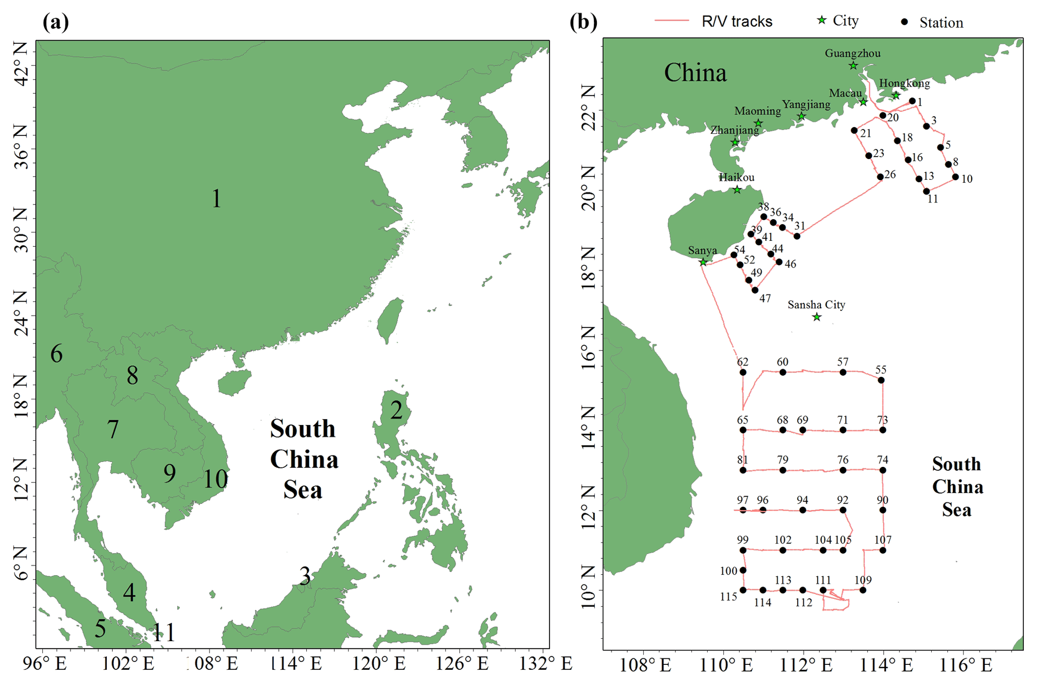
Figure 1 Map of the South China Sea (a) (1: China, 2: Philippines, 3: Brunei, 4: Malaysia, 5: Indonesia, 6: Myanmar, 7: Thailand, 8: Laos, 9: Cambodia, 10: Vietnam, 11: Singapore). The locations of the Pearl River estuary (PRE), DGM sampling stations, and R/V tracks (b). It should be noted that the black solid points represent the sampling stations, while the number near the black solid point represents the name of the station.

2 Materials and methods

2.1 Study area

The SCS is located in the downwind of Southeast Asia (Fig. 1a), and it is the largest semi-enclosed marginal sea in the western tropical Pacific Ocean. The SCS is connected with the East China Sea (ECS) to the northeast and the western Pacific Ocean to the east (Fig. 1a). The SCS is surrounded by numerous developing and developed countries (Fig. 1a). An open cruise was organized by the South China Sea Institute of Oceanology (Chinese Academy of Sciences) and conducted during the period of 3–28 September 2015. The sampling campaign was conducted on R/V Shiyan 3, which departed from Guangzhou, circumnavigated the northern and western SCS, and then returned to Guangzhou. The DGM sampling stations and R/V tracks are plotted in Fig. 1b. In this study, meteorological parameters (including photosynthetically available radiation (PAR) (Li-COR^®, model: Li-250), wind speed, air temperature, and RH) were measured synchronously with atmospheric Hg onboard the R/V.

2.2 Experimental methods

2.2.1 Atmospheric GEM measurements

In this study, GEM was measured using an automatic dual-channel, single-amalgamation cold vapor atomic fluorescence analyzer (model 2537B, Tekran^®, Inc., Toronto, Canada), which has been reported in our previous studies (Wang et al., 2016a, b, c). In order to reduce the contamination from the ship exhaust plume as possible, we installed the Tekran^® system inside the ship's laboratory (the internal air temperature was controlled to 25 ^∘C using an air conditioner) on the fifth deck of the R/V and mounted the sampling inlet at the front deck 1.5 m above the top deck (about 16 m above sea level) using a 7 m heated (maintained at 50 ^∘C) polytetrafluoroethylene (PTFE) tube (0.635 cm in outer diameter). The sampling interval was 5 min and the air flow rate was 1.5 L min⁻¹ in this study. Moreover, two PTFE filters (0.2 µm pore size, 47 mm diameter) were positioned before and after the heated line, and the soda lime before the instrument was changed every 3 d during the cruise. The Tekran^® instrument was calibrated every 25 h using the internal calibration source and these calibrations were checked by injections of a certain volume of saturated Hg⁰ before and after this cruise. The relative percent difference between manual injections and automated calibrations was < 5 %. The precision of the analyzer was determined to > 97 %, and the detection limit was < 0.1 ng m⁻³.

The meteorological and basic seawater parameters were collected onboard the R/V, which was equipped with meteorological and oceanographic instrumentations. To investigate the influence of air mass movements on the GEM levels, 72 h back trajectories of air masses were calculated using the Hybrid Single Particle Lagrangian Integrated Trajectory (HYSPLIT) model (Draxler and Rolph, 2012) and TrajStat software (Wang et al., 2009) based on the Geographic Information System. The Global Data Assimilation System (GDAS) meteorological dataset (ftp://arlftp.arlhq.noaa.gov/pub/archives/gdas1/, last access: 7 August 2019) with $\mathrm{1}{}^{\circ }\times \mathrm{1}{}^{\circ }$ latitude and longitude horizontal spatial resolution and 23 vertical levels at 6 h intervals was used as the HYSPLIT model input. It should be noted that the start time of each back trajectory was identical to the GEM sampling time (UTC) and the start height was set at 500 m above sea level to represent the approximate height of the mixing MBL where atmospheric pollutants were well mixed.

2.2.2 Sampling and analysis of RGM and Hg^P

The Hg${}_{\mathrm{2.5}}^{\mathrm{P}}$ (Hg^P in PM_2.5) was collected on a quartz filter (47 mm in diameter, Whatman), which has been reported in several previous studies (Landis et al., 2002; Liu et al., 2011; Kim et al., 2012). It should be pointed out that the KCl-coated denuders were heated at 500 ^∘C for 1 h and the quartz filters were pre-cleaned by pyrolysis at 900 ^∘C for 3 h to remove the possible pollutant. The RGM and Hg${}_{\mathrm{2.5}}^{\mathrm{P}}$ were sampled using a manual system (URG-3000M), which has been reported in previous studies (Landis et al., 2002; Liu et al., 2011; Wang et al., 2016b). The sampling unit includes an insulated box (Fig. S1 in the Supplement), two quartz annular denuders, two Teflon filter holders (URG Corporation), and a pump. The sampling flow rate was 10 L min⁻¹ (Landis et al., 2002) and the sampling inlet was 1.2 m above the top deck of the R/V. In this study, one Hg${}_{\mathrm{2.5}}^{\mathrm{P}}$ sample was collected in the daytime (06:00–18:00) and the other in the nighttime (18:00–06:00 (next day)), while two RGM samples were collected in the daytime (06:00–12:00 and 12:00–18:00, local time) and one RGM sample in the nighttime. Quality assurance and quality control for Hg^P and RGM were carried out using field blank samples and duplicates. The field blank denuders and quartz filters were treated similarly to the other samples, but not sampling. The mean relative differences of duplicated Hg${}_{\mathrm{2.5}}^{\mathrm{P}}$ and RGM samples (n=6) were 13±6 % and 9±7 %, respectively.

Meanwhile, we collected different size particles using an Andersen impactor (nine-stage), which has been widely used in previous studies (Feddersen et al., 2012; Kim et al., 2012; Zhu et al., 2014; Wang et al., 2016a). The Andersen cascade impactor was installed on the front top deck of the R/V to sample the size-fractionated particles in PM₁₀. In order to diminish the contamination from the exhaust plume of the ship as possible, we turned off the pump when R/V arrived at stations and then switched it back on when the R/V went to the next station. The sample collection began in the morning (10:00) and continued for 2 d with a sampling flow rate of 28.3 L min⁻¹. Field blanks for Hg^P were collected by placing nine pre-cleaned quartz filters (81 mm in diameter, Whatman) in another impactor for 2 d without turning on the pump. After sampling, the quartz filters were placed in cleaned plastic boxes (sealing in Ziploc plastic bags) and then were immediately preserved at −20 ^∘C until the analysis.

The detailed analysis processes of RGM and Hg^P have been reported in our previous studies (Wang et al., 2016a, b). Briefly, the denuder and quartz filter were thermally desorbed at 500 and 900 ^∘C, respectively, and then the resulting thermally decomposed Hg⁰ in carrier gas (zero air, i.e., Hg-free air) was quantified. The method detection limit was calculated to be 0.67 pg m⁻³ for RGM based on 3 times the standard deviation of the blanks (n=57) for the whole dataset. The average field blank value of denuders was 1.2±0.6 pg (n=6), while the average blank values (n=6) of Hg${}_{\mathrm{2.5}}^{\mathrm{P}}$ and Hg${}_{\mathrm{10}}^{\mathrm{P}}$ were 1.4 pg (equivalent of < 0.2 pg m⁻³ for a 12 h sampling time) and 3.2 pg (equivalent of < 0.04 pg m⁻³ for a 2 d sampling time) of Hg per filter, respectively. The detection limits of Hg${}_{\mathrm{2.5}}^{\mathrm{P}}$ and Hg${}_{\mathrm{10}}^{\mathrm{P}}$ were all less than 1.5 pg m⁻³ based on 3 times the standard deviation of field blanks. It should be noted that all the observed RGM and Hg^P values were higher than the corresponding blank values, and the average blank values for RGM and Hg^P were subtracted from the samples.

2.2.3 Determination of DGM in surface seawater

In this study, the analysis was carried out according to the trace element clean technique, and all containers (borosilicate glass bottles and PTFE tubes, joints, and valves) were cleaned prior to use with detergent, followed by trace-metal-grade HNO₃ and HCl, and then rinsed with Milli-Q water (> 18.2 M Ω cm⁻¹), which has been described in our previous study (Wang et al., 2016c). DGM was measured in situ using a manual method (Fu et al., 2010; Ci et al., 2011). The detailed sampling and analysis of DGM has been elaborated in our previous study (Wang et al., 2016c). The analytical blanks were conducted onboard the R/V by extracting Milli-Q water for DGM. The mean concentration of DGM blank was 2.3±1.2 pg L⁻¹ (n=6), accounting for 3 %–10 % of the raw DGM in seawater samples. The method detection limit was 3.6 pg L⁻¹ on the basis of 3 times the standard deviation of system blanks. The relative standard deviation of duplicate samples is generally < 8 % of the mean concentration (n=6).

2.2.4 Estimation of the sea–air exchange flux of Hg⁰

The sea–air flux of Hg⁰ was calculated using a thin film gas exchange model developed by Liss and Slater (1974) and Wanninkhof (1992). The detailed calculation processes of Hg⁰ flux have been reported in recent studies (Ci et al., 2011; Kuss, 2014; Kuss et al., 2018; Wang et al., 2016c). It should be noted that the Schmidt number for gaseous Hg (Sc_Hg) is defined as the following equation: Sc${}_{\mathrm{Hg}}=\mathit{\nu }/D_{\mathrm{Hg}}$, where ν is the kinematic viscosity (cm² s⁻¹) of seawater calculated using the method of Wanninkhof (1992) and D_Hg is the Hg⁰ diffusion coefficient (cm² s⁻¹) in seawater, which is calculated according to recent research (Kuss, 2014). The degree of Hg⁰ saturation (S_a) was calculated using the following equation, $S_a=H^{\prime }{\mathrm{DGM}}_{\mathrm{conc}.}/{\mathrm{GEM}}_{\mathrm{conc}}$, and the calculation of H^′ (the dimensionless Henry's law constant) has been reported in previous studies (Ci et al., 2011, 2015; Kuss, 2014).

Table 1 The GEM, Hg${}_{\mathrm{2.5}}^{\mathrm{P}}$, and RGM concentrations in this study and other literature.

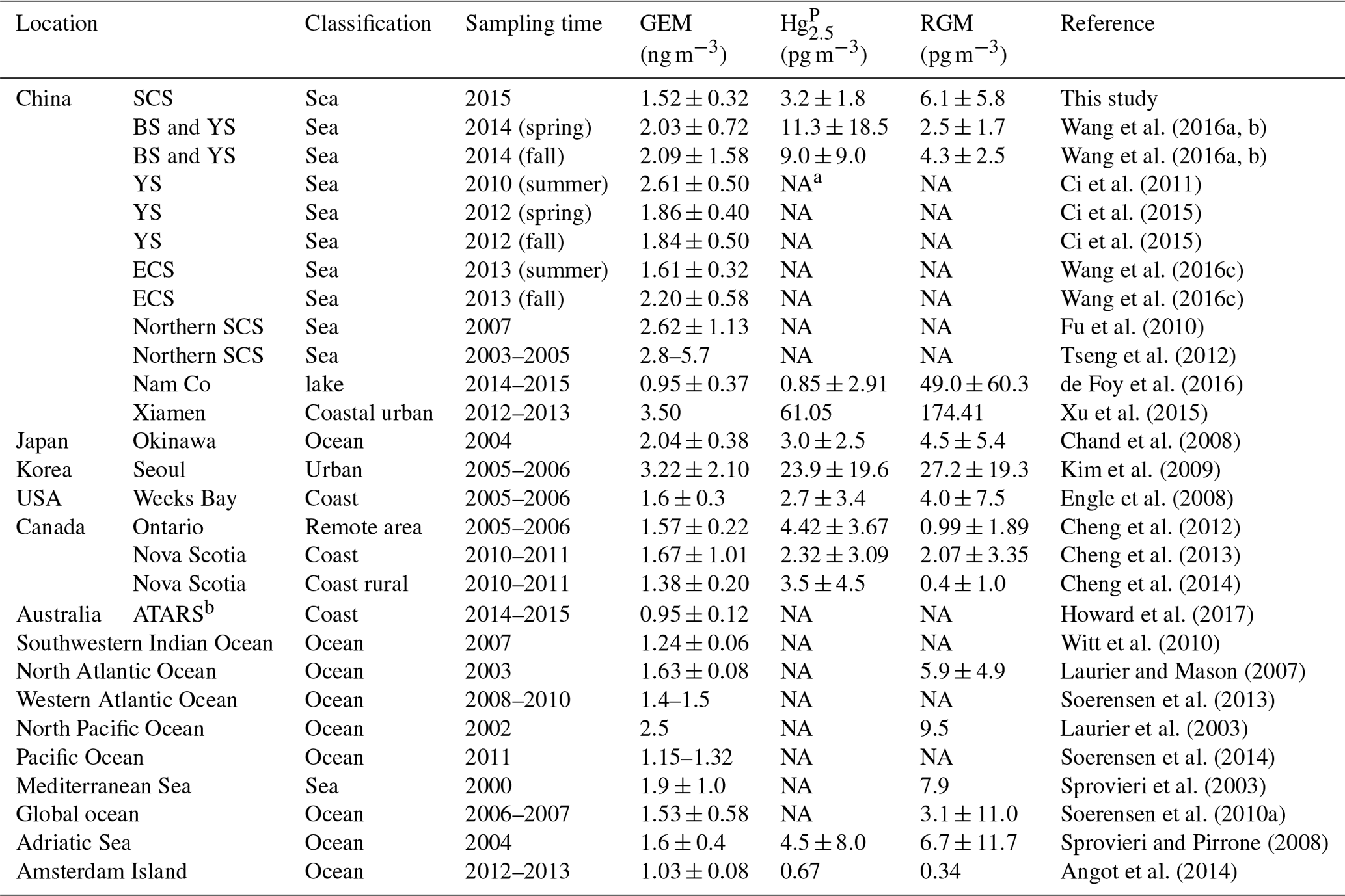
^a NA: No data available. ^b ATARS: Australian Tropical Atmospheric Research Station.

3 Results and discussion

3.1 Speciated atmospheric Hg concentrations

Figure 2 shows the time series of speciated atmospheric Hg and meteorological parameters during the cruise in the SCS. The GEM concentration during the whole study period ranged from 0.92 to 4.12 ng m⁻³ with a mean value of 1.52±0.32 ng m⁻³ (n=4673), which was comparable to the average GEM levels over the global oceans (1.4–1.6 ng m⁻³, Soerensen et al., 2010a, 2013) and Atlantic Ocean (1.63±0.02 ng m⁻³, Laurier and Mason, 2007), higher than those at background sites in the Southern Hemisphere (0.85–1.05 ng m⁻³, Slemr et al., 2015; Howard et al., 2017), and also higher than those in remote oceans, such as the Cape Verde Observatory station (1.19±0.13 ng m⁻³, Read et al., 2017), equatorial Pacific Ocean (1.15–1.05 ng m⁻³, Soerensen et al., 2014), and Indian Ocean (1.0–1.2 ng m⁻³, Witt et al., 2010; Angot et al., 2014), but lower than those in marginal seas, such as the Bohai Sea (BS), Yellow Sea (YS), and ECS (Table 1). However, previous studies conducted in the northern SCS showed that the average GEM concentrations in their study period (2.6–3.5 ng m⁻³, Fu et al., 2010; Tseng et al., 2012) were higher than that in this study. This is due to the fact that the GEM levels in the northern SCS (Fu et al., 2010; Tseng et al., 2012) were considerably higher than that in the western SCS (this study).

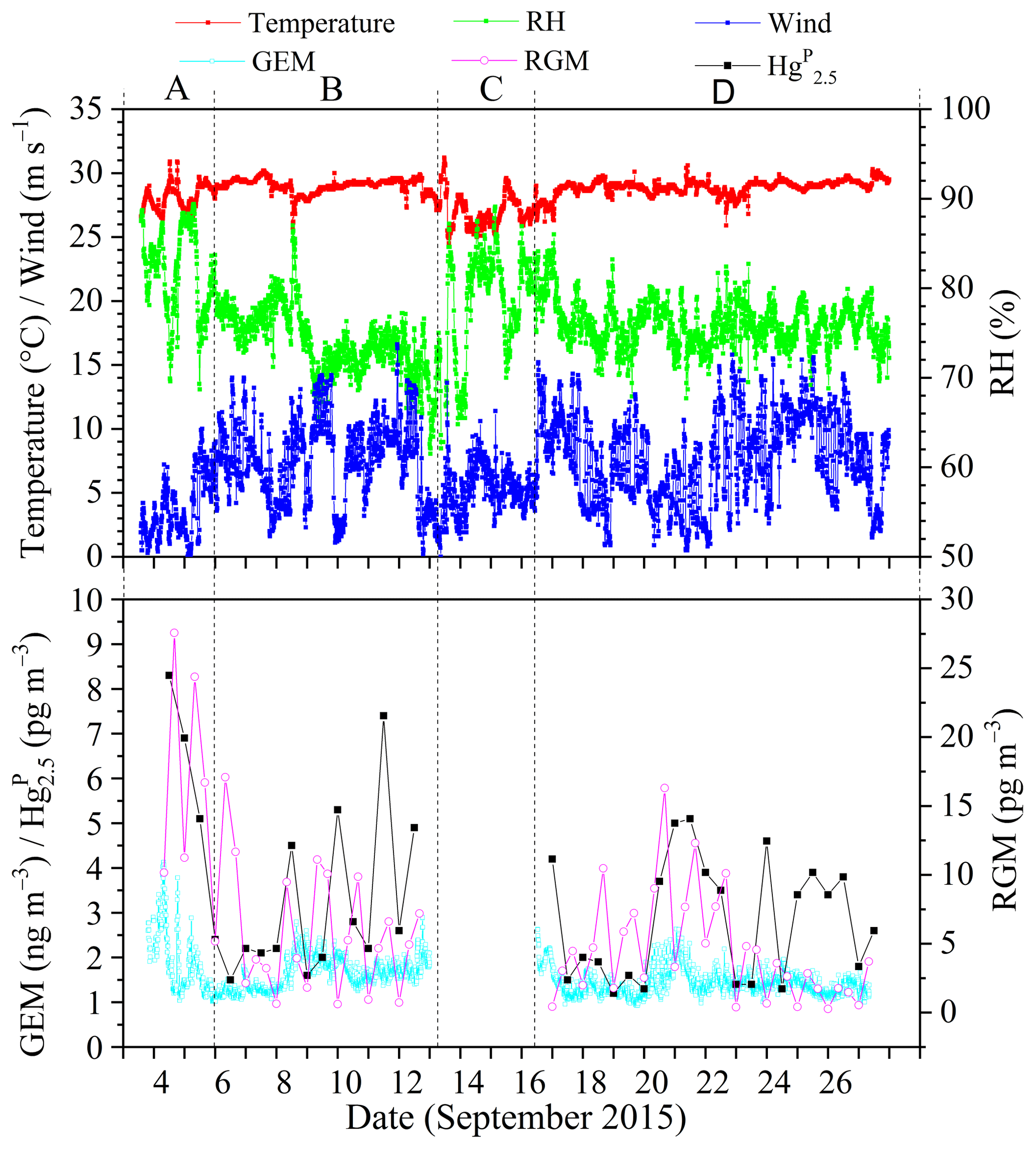
Figure 2 Time (local time) series of GEM, Hg${}_{\mathrm{2.5}}^{\mathrm{P}}$, RGM, and some meteorological parameters, including relative humidity (RH), air temperature, and wind speed (“A” represents the data measured in the PRE, “B” represents the data measured in the northern SCS, “C” represents the data obtained in the port of Sanya, and “D” represents the data measured in the western SCS). It was rainy on the days of 8 and 26 September 2015.

The Hg${}_{\mathrm{2.5}}^{\mathrm{P}}$ concentrations over the SCS ranged from 1.2 to 8.3 pg m⁻³ with a mean value of 3.2±1.8 pg m⁻³ (n=39) (Fig. 2), which was higher than those observed at Nam Co (China) and Amsterdam Island, and were comparable to those in other coastal areas, such as Okinawa, Nova Scotia, the Adriatic Sea, Ontario, and Weeks Bay (see Table 1), but lower than those in the BS and YS (Wang et al., 2016b), and considerably lower than those in rural and urban sites, such as Xiamen, Seoul (see Table 1), Guiyang, and Waliguan (Fu et al., 2011, 2012). The results showed that the SCS suffered less influence from fresh emissions. The RGM concentration over the SCS ranged from 0.27 to 27.57 pg m⁻³ with a mean value of 6.1±5.8 pg m⁻³ (n=58), which was comparable to those in other seas, such as the North Pacific Ocean, North Atlantic Ocean, and Mediterranean Sea (including the Adriatic Sea) (Table 1), higher than the global mean RGM concentration in the MBL (Soerensen et al., 2010a), and also higher than those measured at a few rural sites (Valente et al., 2007; Liu et al., 2010; Cheng et al., 2013, 2014), but significantly much lower than those polluted urban areas in China and South Korea, such as Guiyang (35.7±43.9 pg m⁻³, Fu et al., 2011), Xiamen, and Seoul (Table 1). Furthermore, Fig. 2 shows that the long-lived GEM has smaller variability compared to the short-lived species like RGM and Hg${}_{\mathrm{2.5}}^{\mathrm{P}}$, indicating that atmospheric reactive Hg was easily scavenged from the marine atmosphere, due not only to their characteristics (high activity and solubility), but also due to their sensitivity to meteorological conditions and chemical environments. This pattern was consistent with our previous observed patterns in the BS and YS (Wang et al., 2016b). Moreover, we found that atmospheric reactive Hg represents less than 1 % of TAM in the atmosphere, which was comparable to those measured in other marginal and inner seas, such as the BS and YS (Wang et al., 2016b), the Adriatic Sea (Sprovieri and Pirrone, 2008), and Okinawa (located in the ECS) (Chand et al., 2008), but was significantly lower than those at the urban sites (Table 1).

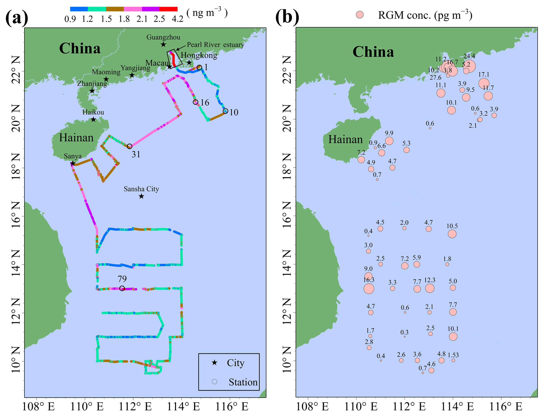
Figure 3 The concentrations and spatial distributions of GEM (a) and RGM (b) in the MBL of the SCS.

3.2 Spatial distribution of atmospheric Hg

3.2.1 Spatial distributions of GEM and RGM

The spatial distribution of GEM over the SCS is illustrated in Fig. 3a. The mean GEM concentration in the northern SCS (1.73±0.40 ng m⁻³ with a range of 1.01–4.12 ng m⁻³) was significantly higher than that in the western SCS (1.41±0.26 ng m⁻³ with a range of 0.92–2.83 ng m⁻³) (t test, p < 0.01). Additionally, we found that the GEM concentrations in the Pearl River estuary (PRE; average value > 2.00 ng m⁻³) were significantly higher than those in the open SCS (see Figs. 2 and 3a), indicating that this nearshore area suffered from high GEM pollution in our study period, probably due to the surrounding human activities. Figure 3a showed that there was a large difference in GEM concentration between stations 1–10 and stations 16–31. The 72 h back trajectories of air masses showed that the air masses with low GEM levels between stations 1 and 10 mainly originated from the SCS (Fig. S2a), while the air masses with high GEM levels at stations 16–31 primarily originated from East China and the ECS and then passed over the southeastern coastal regions of China (Fig. S2b). Additionally, we found that there was small variability of GEM concentrations over the western SCS, except for the measurements near station 79 (Fig. 3a). The back trajectories showed that the air masses with elevated GEM levels near station 79 originated from the south of Taiwan, while the other air masses mainly originated from the western Pacific Ocean (Fig. S3a) and the Andaman Sea (Fig. S3b). Therefore, the air masses dominantly originated from the sea and ocean in this study period, and this could be the main reason for the low GEM level over the SCS. In conclusion, GEM concentrations showed a conspicuous dependence on the sources and movement patterns of air masses during this cruise.

The spatial distribution of the RGM over the SCS is plotted in Fig. 3b. The mean RGM concentration in the northern SCS (7.1±1.4 pg m⁻³) was also obviously higher than that in the western SCS (3.8±0.7 pg m⁻³) (t test, p < 0.05), indicating that a portion of the RGM in the northern SCS maybe originated from the anthropogenic emission. We observed elevated RGM concentrations in the PRE, and this spatial distribution pattern was consistent with that of GEM, indicating that part of the RGM near PRE probably originated from the surrounding human activities. This is confirmed by the following fact: the RGM concentrations in nighttime of the 2 d in the PRE were 11.3 and 5.2 pg m⁻³ (Figs. 3b and S4), and they were significantly higher than those in the open SCS. Another obvious feature was that the amplitude of the RGM concentration was much greater than the GEM, and this further indicated that the RGM was easily removed from the atmosphere through both the wet and dry deposition. In addition, we found that the RGM concentrations in the nearshore area were not always higher than those in the open sea, except for the measurements in the PRE, suggesting that the RGM in the remote marine atmosphere presumably did not originate from land but from the in situ photo-oxidation of Hg⁰, which had been reported in previous studies (e.g., Hedgecock and Pirrone, 2001; Lindberg et al., 2002; Laurier et al., 2003; Sprovieri et al., 2003, 2010; Sheu and Mason, 2004; Laurier and Mason, 2007; Soerensen et al., 2010a; Wang et al., 2015).

3.2.2 Spatial distributions of Hg${}_{\mathrm{2.5}}^{\mathrm{P}}$ and Hg${}_{\mathrm{10}}^{\mathrm{P}}$

The concentrations and spatial distribution of Hg${}_{\mathrm{2.5}}^{\mathrm{P}}$ in the MBL are illustrated in Fig. 4a. The highest Hg${}_{\mathrm{2.5}}^{\mathrm{P}}$ value (8.3 pg m⁻³) was observed in the PRE during daytime on 4 September 2015, presumably due to the local human activities. The homogeneous distribution and lower level of Hg${}_{\mathrm{2.5}}^{\mathrm{P}}$ in the open SCS indicated that the Hg${}_{\mathrm{2.5}}^{\mathrm{P}}$ did not originate from the land and that the SCS suffered less influence from human activities, especially in the open sea. This is due to the fact that the majority of air masses in the SCS during this study period came from the seas and oceans. The spatial distribution pattern of Hg${}_{\mathrm{2.5}}^{\mathrm{P}}$ in this study was different from our previous observed patterns in the BS and YS (Wang et al., 2016b), which showed that Hg${}_{\mathrm{2.5}}^{\mathrm{P}}$ concentrations in the nearshore area were higher than those in the open sea in both spring and fall, mainly due to the outflow of atmospheric Hg^P from East China.

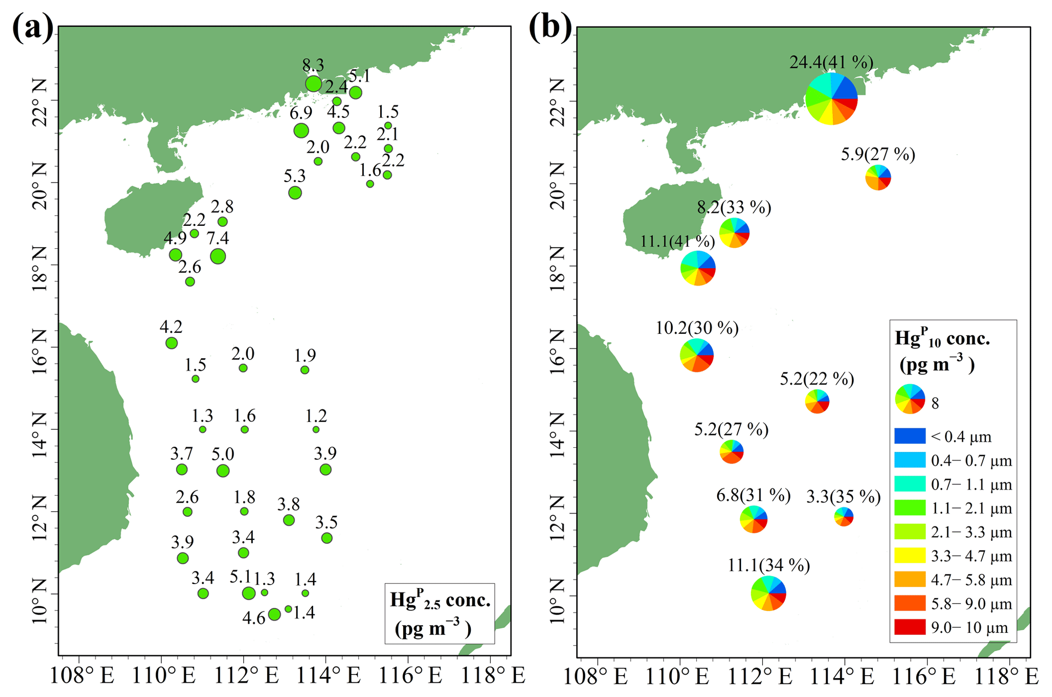
Figure 4 Spatial distributions of Hg${}_{\mathrm{2.5}}^{\mathrm{P}}$ (a) and Hg${}_{\mathrm{10}}^{\mathrm{P}}$ (Hg${}_{\mathrm{2.1}}^{\mathrm{P}}$ ∕ Hg${}_{\mathrm{10}}^{\mathrm{P}}$ ratio) (b) in the MBL of the SCS. Hg${}_{\mathrm{2.5}}^{\mathrm{P}}$, Hg${}_{\mathrm{2.1}}^{\mathrm{P}}$, and Hg${}_{\mathrm{10}}^{\mathrm{P}}$ denote the Hg^P in PM_2.5, PM_2.1, and PM₁₀, respectively.

The concentrations and spatial distributions of Hg${}_{\mathrm{10}}^{\mathrm{P}}$ in the MBL of the SCS are illustrated in Fig. 4b. We found that the Hg${}_{\mathrm{10}}^{\mathrm{P}}$ concentration was considerably (1–6 times) higher in the PRE than those of other regions of the SCS, probably due to the large emissions of anthropogenic Hg in surrounding areas of the PRE. Moreover, the highest Hg${}_{\mathrm{2.1}}^{\mathrm{P}}$ ∕ Hg${}_{\mathrm{10}}^{\mathrm{P}}$ ratio (41 %) was observed in the PRE and coastal sea area of Hainan, while the lowest ratio (22 %) was observed in the open sea (Fig. 4b). The Hg${}_{\mathrm{10}}^{\mathrm{P}}$ concentrations and Hg${}_{\mathrm{2.1}}^{\mathrm{P}}$ ∕ Hg${}_{\mathrm{10}}^{\mathrm{P}}$ ratios were higher in the nearshore area compared to those in the open sea, demonstrating that coastal sea areas are polluted by anthropogenic Hg to a certain extent. Interestingly, we found the mean Hg${}_{\mathrm{2.1}}^{\mathrm{P}}$ concentration (3.16±2.69 pg m⁻³, n=10) measured using the Andersen sampler was comparable to the mean Hg${}_{\mathrm{2.5}}^{\mathrm{P}}$ concentration (3.33±1.89 pg m⁻³, n=39) measured using a 47 mm Teflon filter holder (t test, p > 0.1). This indicated that the fine Hg^P level in the MBL of the SCS was indeed low, and there might be no significant difference in Hg^P concentration in the SCS between 12 and 48 h sampling time.

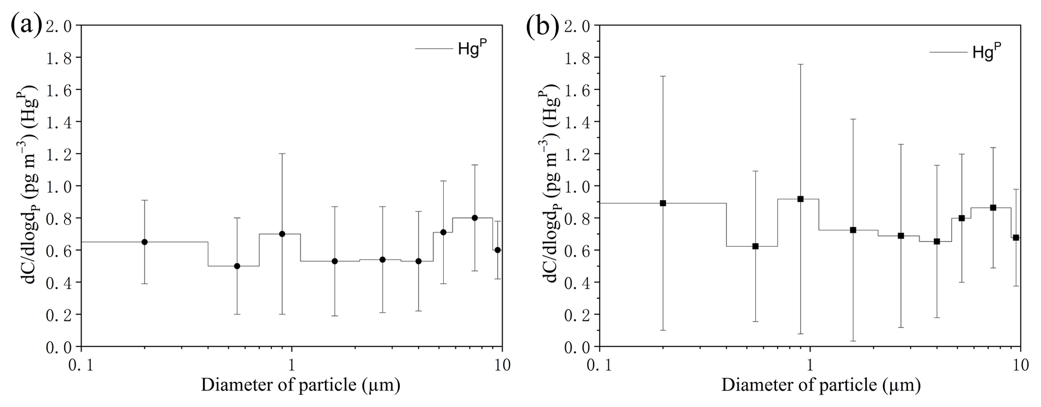
Figure 5 Size-distributed concentrations of Hg^P (PM₁₀) in the MBL of the SCS. (a) represents all the data excepting the measurements in the PRE; (b) represents all the data. The data shown are the mean and standard error.

The concentrations of all size-fractionated Hg^P are summarized in Table S1 in the Supplement. The size distribution of Hg^P in the MBL of the SCS is plotted in Fig. 5. One striking feature was that the three-modal pattern with peaks around < 0.4, 0.7–1.1, and 5.8–9.0 µm was observed for the size distributions of Hg^P in the open sea (Fig. 5a) if we excluded the data in the PRE. The three-modal pattern was more obvious when we consider all the data (Fig. 5b). Generally, the Hg^P concentrations in coarse particles were significantly higher than those in fine particles, and Hg${}_{\mathrm{2.1}}^{\mathrm{P}}$ contributed approximately 32 % (22 %–41 %; see Fig. 4b) to the Hg${}_{\mathrm{10}}^{\mathrm{P}}$ for all the data, indicating that the coarse mode was the dominant size during this study period. This might be explained by the sources of the air masses. Since air masses dominantly originated from the sea and ocean (Figs. S1 and S2) and contained high concentrations of sea salts, which generally exist in the coarse mode (1–10 µm) (Athanasopoulou et al., 2008; Mamane et al., 2008), the Hg${}_{\mathrm{2.1}}^{\mathrm{P}}$ ∕ Hg${}_{\mathrm{10}}^{\mathrm{P}}$ ratios were generally lower in the SCS compared to those in the BS, YS, and ECS (Wang et al., 2016a).

3.3 Dry deposition fluxes of RGM and Hg^P

The dry deposition flux of Hg${}_{\mathrm{10}}^{\mathrm{P}}$ was obtained by summing the dry deposition fluxes of each size-fractionated Hg^P in the same set. The dry deposition flux of Hg${}_{\mathrm{10}}^{\mathrm{P}}$ is calculated using the following equation: $F=\sum C$Hg^P×V_d; F is the dry deposition flux of Hg${}_{\mathrm{10}}^{\mathrm{P}}$ (ng m⁻² d⁻¹), CHg^P is the concentration of Hg^P in each size fraction (pg m⁻³), and V_d is the corresponding dry deposition velocity (cm s⁻¹). In this study, the dry deposition velocities of 0.03, 0.01, 0.06, 0.15, and 0.55 cm s⁻¹ (Giorgi, 1988; Pryor et al., 2000; Nho-Kim et al., 2004) were chosen for the following size-fractionated particles: < 0.4, 0.4–1.1, 1.1–2.1, 2.1–5.8, and 5.8–10 µm, respectively (Wang et al., 2016a). The average dry deposition flux of Hg${}_{\mathrm{10}}^{\mathrm{P}}$ was estimated to be 1.08 ng m⁻² d⁻¹ based on the average concentration of each size-fractionated Hg^P in the SCS (Table S2), which was lower than those in the BS, YS, and ECS (Wang et al., 2016a). The dry deposition velocity of RGM was 4.0–7.6 cm s⁻¹ because of its characteristics and rapid uptake by sea-salt aerosols followed by deposition (Poissant et al., 2004; Selin et al., 2007). The annual dry deposition fluxes of Hg${}_{\mathrm{10}}^{\mathrm{P}}$ and RGM to the SCS were calculated to be 1.42 and 27.39–52.05 t yr⁻¹ based on the average Hg${}_{\mathrm{10}}^{\mathrm{P}}$ and RGM concentrations and the area of the SCS (3.56×10¹² m²). The result showed that RGM contributed more than 95 % to the total dry deposition of atmospheric reactive Hg. The annual dry deposition flux of RGM was considerably higher than that of the Hg${}_{\mathrm{10}}^{\mathrm{P}}$ due to the higher deposition rate and concentration of RGM in the SCS.

3.4 Temporal variation of atmospheric Hg

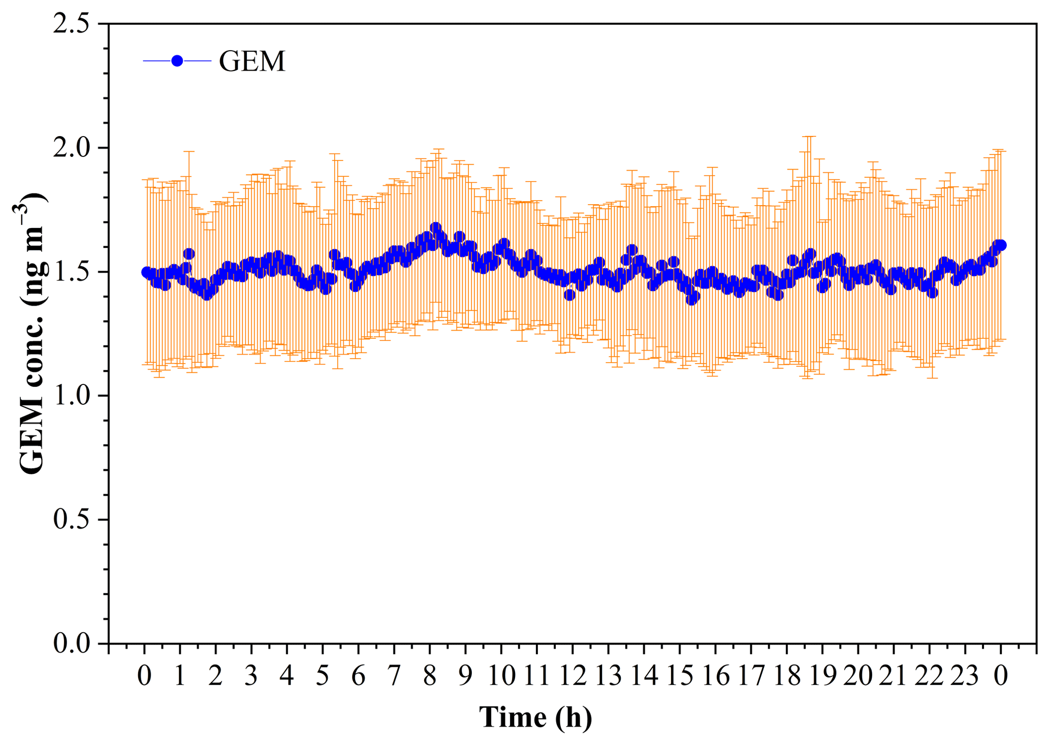
3.4.1 Diurnal variation of GEM

The diurnal variation of GEM concentration during the whole study period is illustrated in Fig. 6. It was notable that there was no significant variability of the mean (± SD) GEM concentration in a whole day during this study period, and the GEM concentration dominantly fell in the range of 1.3–1.7 ng m⁻³ (Fig. 6). The statistical result showed that the mean GEM concentration in the daytime (06:00–18:00) (1.49±0.06 pg m⁻³) was comparable to that in the nighttime (1.51±0.06 pg m⁻³) (t test, p > 0.05). The lower GEM concentrations and smaller variability over the SCS further revealed that the SCS suffered less influence of fresh emissions.

Figure 6 Diurnal variation of GEM concentration (mean ± SD) over the SCS.

3.4.2 Daily variation of RGM

The average RGM concentrations in the daytime and nighttime are illustrated in Fig. 7. Firstly, we found that RGM showed a diurnal variation with higher concentrations in the daytime and lower concentrations in the nighttime during the whole study period. The mean RGM concentration in the daytime (8.0±5.5 pg m⁻³) was significantly and considerably higher than that in the nighttime (2.2±2.7 pg m⁻³) (t test, p < 0.001). This diurnal pattern was in line with the previous studies (Laurier and Mason, 2007; Liu et al., 2007; Engle et al., 2008; Cheng et al., 2014). This is due to the fact that the oxidation of GEM in the MBL must be photochemical, which has been shown by the diurnal cycle of RGM (Laurier and Mason, 2007). Another reason was that there was more Br (gas phase) production during daytime (Sander et al., 2003). Figure S3 showed that the RGM concentration in the nighttime was lower than those in the corresponding forenoon and afternoon, except for the measurements in the PRE. This further indicated that (1) the RGM originated from the photo-oxidation of Hg⁰ in the atmosphere and (2) the transfer of RGM to Hg^P due to higher RH and lower air temperature in nighttime (Rutter and Schauer, 2007; Lee et al., 2016).

Figure 7 Daily variation of RGM concentration over the SCS.

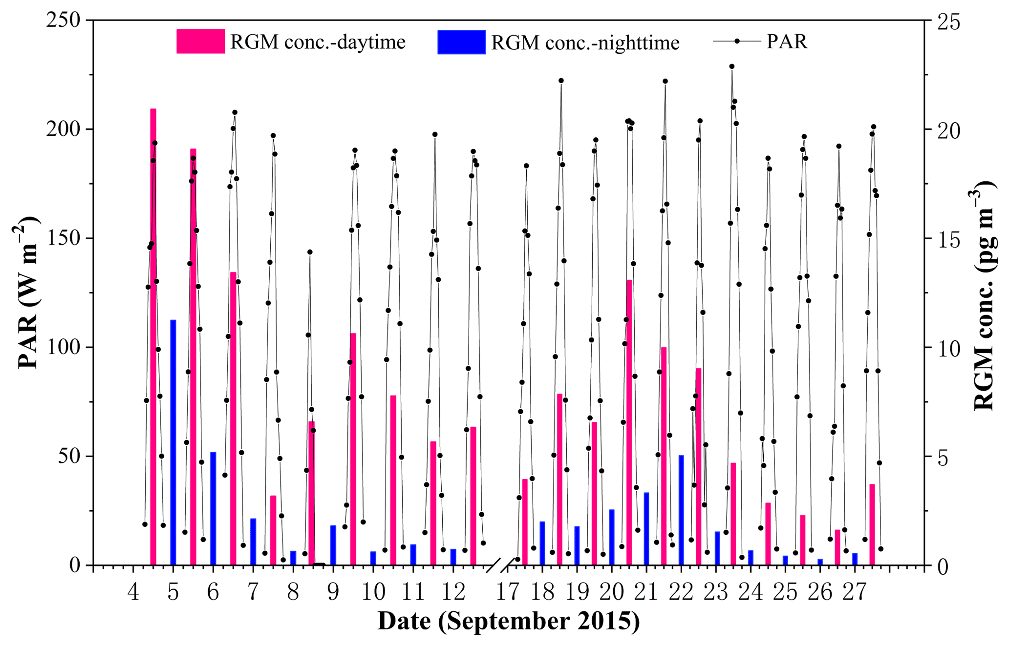
In addition, we found that the difference in RGM concentration between day and night in the SCS was higher than those in the BS and YS (Wang et al., 2016b), and one possible reason was that the solar radiation and air temperature over the SCS were stronger and higher compared to those over the BS and YS (Wang et al., 2016b) as a result of the specific location of the SCS (tropical sea) and the different sampling season (the SCS: September 2015; the BS and YS: April–May and November 2014). Secondly, we found that the higher the RGM concentrations in the daytime, the higher the RGM concentrations in the nighttime, but the concentrations in daytime were higher than that in the corresponding nighttime throughout the sampling period (see Figs. 7 and S3). This is partly because the higher RH and lower air temperature in nighttime were conducive to the removal of RGM (Rutter and Schauer, 2007; Amos et al., 2012). Thirdly, we found that the difference in RGM concentration between different days was large, though there was no significant difference in PAR values (Fig. 7). However, here again are two kinds of cases: the first kind of circumstance was that the higher RGM in the PRE (day and night) presumably mainly originated from the surrounding human activities (i.e., 4–5 September 2015), and the second scenario was that RGM in open waters mainly originated from the in situ oxidation of GEM in the MBL (Soerensen et al., 2010a; Sprovieri et al., 2010). The main reason for the large difference in RGM concentration between different days was that there was a large difference in wind speed and RH between different days (see Fig. 2), and the discussion can be found in the following paragraphs.

3.4.3 Daily variation of Hg${}_{\mathrm{2.5}}^{\mathrm{P}}$

Figure 8 shows the Hg${}_{\mathrm{2.5}}^{\mathrm{P}}$ concentrations in the daytime and nighttime during the entire study period. The Hg${}_{\mathrm{2.5}}^{\mathrm{P}}$ value in the daytime (3.4±1.9 pg m⁻³, n=20) was slightly but not significantly higher than that in the nighttime (2.4±0.9 pg m⁻³, n=19) (t test, p > 0.1), and this pattern was consistent with the result of our previous study conducted in the open waters of the YS (Wang et al., 2016b). The elevated Hg${}_{\mathrm{2.5}}^{\mathrm{P}}$ concentrations in the PRE and nearshore area of Hainan (Figs. 4 and 8) indicated that the nearshore areas were readily polluted due to the anthropogenic Hg emissions, while the low Hg${}_{\mathrm{2.5}}^{\mathrm{P}}$ level in the open sea further suggested that the open areas of the SCS suffered less anthropogenic Hg^P. Therefore, we speculated that the Hg${}_{\mathrm{2.5}}^{\mathrm{P}}$ over the open SCS mainly originated from the in situ formation.

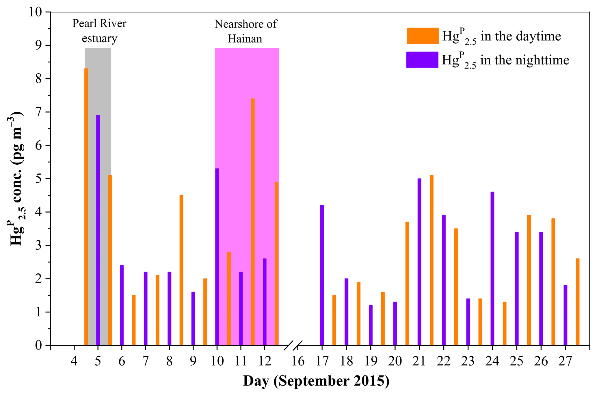
Figure 8 Daily variation of Hg${}_{\mathrm{2.5}}^{\mathrm{P}}$ in the MBL of the SCS. The light gray area represents the data in the PRE, while the light magenta area represents the data in the nearshore area of Hainan.

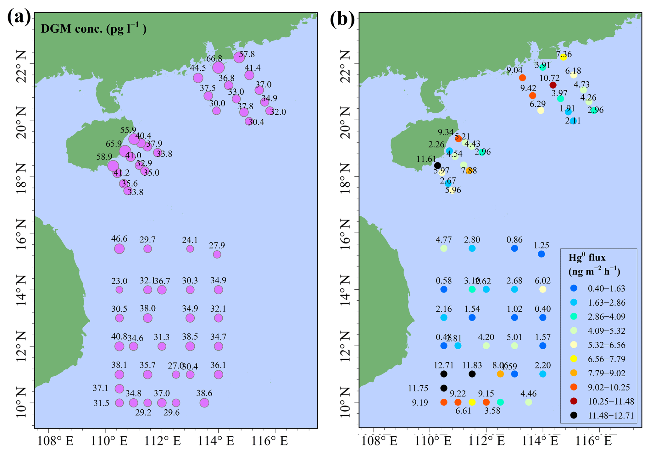
Figure 9 DGM concentrations (a) and sea–air exchange flux of Hg⁰ (b) in the SCS.

During the cruise in the western SCS (16–28 September 2015), we found elevated Hg${}_{\mathrm{2.5}}^{\mathrm{P}}$ concentrations when the RGM concentrations were high at lower wind speed (e.g., 20–22 September 2015: it was sunny on all these days) (see Figs. 2, 7, and 8). This is probably due to the transferal of RGM from the gas to the particle phase. In contrast, we found that the Hg${}_{\mathrm{2.5}}^{\mathrm{P}}$ concentrations were elevated when the RGM concentrations were low at higher wind speed (e.g., 25–27 September 2015: it was cloudy on these days, and there was a transitory drizzle on 26 September 2015) (see Figs. 2, 7, and 8). On the one hand, high wind speed may increase the levels of halogen atoms (Br, Cl, etc.) and sea-salt aerosols in the marine atmosphere, which in turn were favorable for the production of RGM and formation of Hg${}_{\mathrm{2.5}}^{\mathrm{P}}$ (Auzmendi-Murua et al., 2014). On the other hand, high wind speed was favorable for the removal of RGM and Hg${}_{\mathrm{2.5}}^{\mathrm{P}}$ in the atmosphere; this was probably the reason for lower RGM and Hg${}_{\mathrm{2.5}}^{\mathrm{P}}$ concentrations during 25–27 September as compared to those observed during 20–22 September (see Figs. 2, 7, and 8).

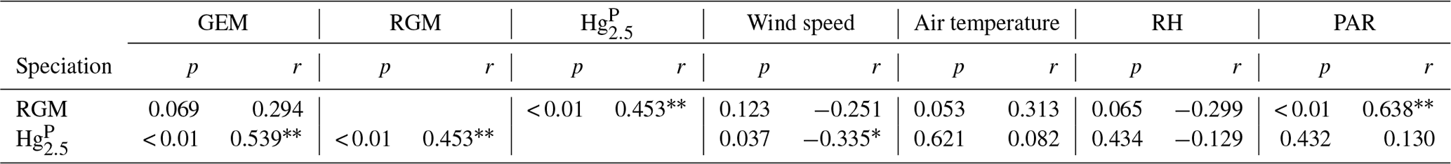
Table 2 Correlation coefficients for speciated atmospheric Hg and meteorological parameters (one asterisk denotes significant correlation in p < 0.05, and double asterisks denote significant correlation in p < 0.01).

3.5 Relationship between atmospheric Hg and meteorological parameters

Pearson's correlation coefficients were calculated between speciated Hg and meteorological parameters to identify the relationships between them (Table 2). According to the correlation analysis, the Hg${}_{\mathrm{2.5}}^{\mathrm{P}}$ was significantly positively correlated with RGM. Part of the reason was that RGM could be adsorbed by particulate matter under high RGM concentrations and then enhanced the Hg^P concentrations. Similarly, the Hg${}_{\mathrm{2.5}}^{\mathrm{P}}$ had a significantly positive correlation with GEM. On the one hand, GEM and Hg^P probably originated from the same sources (including but not limited to anthropogenic and oceanic sources), especially in the PRE and nearshore areas. On the other hand, it was probably due to the fact that GEM could be oxidized to form RGM and then Hg^P, which might be the reason for the positive but not significant correlation between RGM and GEM since a higher GEM level may result in a higher RGM level in daytime.

The correlation analysis showed that the Hg${}_{\mathrm{2.5}}^{\mathrm{P}}$ and RGM were all negatively correlated with wind speed and RH (Table 2), and the higher wind speed was favorable for the removal of Hg${}_{\mathrm{2.5}}^{\mathrm{P}}$ over the RGM. This is because the high wind speed might increase the RH levels and then elevated wind speed and RH may accelerate the removal of Hg${}_{\mathrm{2.5}}^{\mathrm{P}}$ and RGM (Cheng et al., 2014; Wang et al., 2016b). Moreover, both the air temperature and PAR were positively correlated with RGM and Hg${}_{\mathrm{2.5}}^{\mathrm{P}}$. However, the significantly positive correlation between PAR and RGM indicated that the role of solar radiation played in the production of RGM was more obvious than that in the formation of Hg${}_{\mathrm{2.5}}^{\mathrm{P}}$, which was consistent with the previous study at coastal and marine sites (Mao et al., 2012).

3.6 Sea–air exchange of Hg⁰ in the SCS

The spatial distributions of DGM and Hg⁰ fluxes in the SCS are illustrated in Fig. 9. The DGM concentrations in the nearshore area (40–55 pg L⁻¹) were about twice as high as those in the open sea, and this pattern was similar to our previous study conducted in the ECS (Wang et al., 2016c). The DGM concentration in this study varied from 23.0 to 66.8 pg L⁻¹ with a mean value of 37.1±9.0 pg L⁻¹ (Fig. 9a and Table S3), which was higher than those in other open oceans, such as the Atlantic Ocean (11.6±2.0 pg L⁻¹, Anderson et al., 2011) and South Pacific Ocean (9−21 pg L⁻¹, Soerensen et al., 2014), but considerably lower than that in Minamata Bay (116±76 pg L⁻¹, Marumoto and Imai, 2015). The mean DGM concentration in the northern SCS (41.3±10.9 pg L⁻¹) was significantly higher than that in the western SCS (33.5±5.0 pg L⁻¹) (t test, p < 0.01). The reason was that DGM concentrations in the nearshore areas of the PRE and Hainan were higher than those in the western open sea (see Fig. 9a). The DGM in surface seawater of the SCS was supersaturated, with a saturation of 501 % to 1468 % with a mean value of 903±208 %, which was approximately two-thirds of that measured in the ECS (Wang et al., 2016c). The result indicated that (1) the surface seawater in the SCS was supersaturated with gaseous Hg and (2) Hg⁰ evaporated from the surface seawater to the atmosphere during our study period.

The sea–air exchange fluxes of Hg⁰ at all stations were presented in Table S3, including GEM, DGM, PAR, surface seawater temperature, wind speed, and saturation of Hg⁰. Sea–air exchange fluxes of Hg⁰ in the SCS ranged from 0.40 to 12.71 ng m⁻² h⁻¹ with a mean value of 4.99±3.32 ng m⁻² h⁻¹ (Fig. 9b and Table S3), which was comparable to the previous measurements obtained in the Mediterranean Sea, northern SCS, and western Atlantic Ocean (Andersson et al., 2007; Fu et al., 2010; Soerensen et al., 2013) but lower than those in polluted marine environments, such as Minamata Bay, Tokyo Bay, and the YS (Narukawa et al., 2006; Ci et al., 2011; Marumoto and Imai, 2015), while higher than those in some open sea environments, such as the Baltic Sea, Atlantic Ocean, and South Pacific Ocean (Kuss and Schneider, 2007; Kuss et al., 2011; Andersson et al., 2011; Soerensen et al., 2014). Interestingly, we found that the Hg⁰ flux near station 99 was higher than those in open water as a result of higher wind speed (Table S3).

In order to better understand the important role of the SCS, we relate the Hg⁰ flux in the SCS to the global estimation; an annual sea–air flux of Hg⁰ was calculated based on the assumption that there was no seasonal variation in Hg⁰ emission flux from the SCS. The annual emission flux of Hg⁰ from the SCS was estimated to be 159.6 t yr⁻¹ assuming the area of the SCS was 3.56×10¹² m² (accounting for about 1.0 % of the global ocean area), which constituted about 5.5 % of the global Hg⁰ oceanic evasion (Strode et al., 2007; Soerensen et al., 2010b; UNEP, 2013). We attributed the higher Hg⁰ flux in the SCS to the specific location of the SCS (tropical sea) and the higher DGM concentrations in the SCS (especially in the northern area). Therefore, the SCS may actually play an important role in the global Hg oceanic cycle. Additionally, we found that the percentage of the annual dry deposition flux of atmospheric reactive Hg to the annual evasion flux of Hg⁰ was approximately 18 %–34 %, indicating that the dry deposition of atmospheric reactive Hg was an important pathway for the atmospheric Hg to the ocean.

4 Conclusions

During the cruise aboard the R/V Shiyan 3 in September 2015, GEM, RGM, and Hg^P were determined in the MBL of the SCS. The GEM level in the SCS was comparable to the background level over the global oceans due to the air masses dominantly originating from seas and oceans. GEM concentrations were closely related to the sources and movement patterns of air masses during this cruise. Moreover, the speciated atmospheric Hg level in the PRE was significantly higher than those in the open SCS due to the fresh emissions. The Hg^P concentrations in coarse particles were significantly higher than those in fine particles, and the coarse modal was the dominant size, although there were three peaks for the size distribution of Hg^P in PM₁₀, indicating that most of the Hg${}_{\mathrm{10}}^{\mathrm{P}}$ originated from in situ production. There was no significant difference in GEM and Hg${}_{\mathrm{2.5}}^{\mathrm{P}}$ concentrations between day and night, but RGM concentrations were significantly higher in daytime than in nighttime. RGM was positively correlated with PAR and air temperature but negatively correlated with wind speed and RH. The DGM concentrations in nearshore areas of the SCS were higher than those in the open sea, and the surface seawater of the SCS was supersaturated with respect to Hg⁰. The annual flux of Hg⁰ from the SCS accounted for about 5.5 % of the global Hg⁰ oceanic evasion, although the area of the SCS just represents 1.0 % of the global ocean area, suggesting that the SCS played an important role in the global Hg cycle. Additionally, the dry deposition of atmospheric reactive Hg was a momentous pathway for the atmospheric Hg to the ocean because it happens all the time.

Appendix A: List of acronyms and symbols.

Abbreviation	Full name
BS	Bohai Sea
YS	Yellow Sea
ECS	East China Sea
SCS	South China Sea
PRE	Pearl River estuary
MBL	Marine boundary layer
GEM	Gaseous elemental mercury
RGM	Reactive gaseous mercury
TAM	Total atmospheric mercury
Hg${}_{\mathrm{2.1}}^{\mathrm{P}}$	Particulate mercury in PM2.1
Hg${}_{\mathrm{2.5}}^{\mathrm{P}}$	Particulate mercury in PM2.5
Hg${}_{\mathrm{10}}^{\mathrm{P}}$	Particulate mercury in PM10
DGM	Dissolved gaseous mercury