the Creative Commons Attribution 4.0 License.
the Creative Commons Attribution 4.0 License.
 | 08 Jun 2018
Bifurcation of potential vorticity gradients across the Southern Hemisphere stratospheric polar vortex
Jonathan Conway
Greg Bodeker
Chris Cameron
The wintertime stratospheric westerly winds circling the Antarctic continent, also known as the Southern Hemisphere polar vortex, create a barrier to mixing of air between middle and high latitudes. This dynamical isolation has important consequences for export of ozone-depleted air from the Antarctic stratosphere to lower latitudes. The prevailing view of this dynamical barrier has been an annulus compromising steep gradients of potential vorticity (PV) that create a single semi-permeable barrier to mixing. Analyses presented here show that this barrier often displays a bifurcated structure where a double-walled barrier exists. The bifurcated structure manifests as enhanced gradients of PV at two distinct latitudes – usually on the inside and outside flanks of the region of highest wind speed. Metrics that quantify the bifurcated nature of the vortex have been developed and their variation in space and time has been analysed. At most isentropic levels between 395 and 850 K, bifurcation is strongest in mid-winter and decreases dramatically during spring. From August onwards a distinct structure emerges, where elevated bifurcation remains between 475 and 600 K, and a mostly single-walled barrier occurs at other levels. While bifurcation at a given level evolves from month to month, and does not always persist through a season, interannual variations in the strength of bifurcation display coherence across multiple levels in any given month. Accounting for bifurcation allows the region of reduced mixing to be better characterised. These results suggest that improved understanding of cross-vortex mixing requires consideration of the polar vortex not as a single mixing barrier but as a barrier with internal structure that is likely to manifest as more complex gradients in trace gas concentrations across the vortex barrier region.
- Article
(4266 KB) - Full-text XML
- BibTeX
- EndNote


The polar vortex is the defining dynamical feature of the stratosphere during winter and early spring. The steep gradients in trace gas concentrations and in dynamical tracers such as potential vorticity (PV) across the vortex boundary region indicate a dynamical barrier to the mixing of air between the mid-latitude and the high-latitude stratosphere (e.g. Schoeberl et al., 1992; Hoskins et al., 1985; Plumb and Ko, 1992). In the Southern Hemisphere, during winter and spring, the barrier isolates the cold stratospheric air that develops during the polar night from warmer mid-latitude air. The polar stratospheric clouds that form in this region provide the conditions needed for the heterogenous chemical reactions that create the halogen radicals that go on to deplete ozone (Solomon, 1999 and references therein). In springtime, the barrier prevents ozone-depleted air within the Southern Hemisphere polar vortex from mixing with ozone-rich air that accumulates in the downward branch of the Brewer–Dobson circulation equatorward of the vortex. By defining the location of the polar vortex in equivalent latitude (EL) coordinates (Butchart and Remsberg, 1986), the temporal evolution of the size and strength of this dynamical containment of ozone depletion can be assessed (e.g. Bodeker et al., 2002) and periodic mixing of air masses into and out of the vortex can be identified (e.g. Schoeberl and Newman, 1995; Paparella et al., 1997; Ajtic et al., 2004, Manney et al., 2005). Providing a quantitative description of the vortex barrier also allows for the representation of the polar vortex in coupled chemistry–climate models to be evaluated (e.g. Struthers et al., 2009).
The centre of the vortex boundary region is most often defined as (i) the EL of the maximum gradient of PV with respect to EL (herein referred to as PV gradient), with the caveat that the true peak is also located in the region of the maximum westerly jet (e.g. Nash et al., 1996), or (ii) the EL of the maximum of the PV gradient times the average wind speed (e.g. Bodeker et al., 2002; Manney et al., 2007). The inner and outer edges of the vortex boundary region can be assessed using the change in the curvature of the vortex definition function (PV gradient or PV gradient times wind speed). Because there is a one-to-one correspondence between PV values and EL (see Fig. 1a of Nash et al., 1996), the PV values corresponding to the vortex boundary region can be used to map the size and location of the vortex in latitude–longitude coordinates. Methods to map the vortex in two dimensions often use climatological PV values corresponding to the vortex boundary (e.g. Waugh and Randel, 1999; Manney and Lawrence, 2016) because PV gradients exhibit large temporal variability and because the vortex is sometimes poorly defined. Analyses using climatological PV values can represent interannual variations in vortex attributes well, but may not represent the size of the Southern Hemisphere polar vortex well during the spring, as the PV value associated with the strongest PV gradients changes (e.g. Waugh and Randel, 1999). Besides diagnostics using PV gradients, the vortex boundary can also be defined using maximum wind speed in longitudinal bins (e.g. Rummukainen et al., 1994), maximum kinetic energy (e.g. Paparella et al., 1997), concentrations of long-lived trace gases (e.g. McDonald and Smith, 2013), Lagrangian metrics such as Lyapunov exponents or function M (e.g. Garny et al., 2007; Smith and McDonald, 2014; Serra et al., 2017), the complexity of tracer gradients through effective diffusivity (e.g. Haynes and Shuckburgh, 2000), or a combination of different metrics (e.g. Manney and Lawrence, 2016; Lawrence and Manney, 2018). Because of the minimal computational requirements and its basis as a dynamical constraint on mixing, the PV gradient is an attractive method to define the vortex boundary region.
The increased resolution of recent reanalyses (Fujiwara et al., 2017) now allows us to resolve the structure of PV gradients in EL coordinates around the polar vortex in much finer detail than was available when the Nash et al. (1996) definition was proposed. This paper investigates PV gradients during late winter and spring over the altitude range where the highest rates of Southern Hemisphere ozone depletion occur (mid-stratosphere). The aim of this paper is to characterise, in detail, PV gradients across the Southern Hemisphere polar vortex dynamical barrier within the mid-stratosphere, including the vertical and latitudinal structure, seasonal evolution and internal structure of the vortex boundary region.
2.1 Data sets
The primary data set used in this paper is the ERA-Interim reanalysis (Dee et al., 2011) produced by the European Centre for Medium-Range Weather Forecasting (ECMWF). This reanalysis uses a 4-D variational assimilation system to combine observed climate variables in a dynamically consistent fashion. Zonal and meridional wind speed, and Ertel PV data were downloaded on nine potential temperature (Θ) levels (350, 370, 395, 430, 475, 530, 600, 700, 850 K) from the ECMWF online archive on a regular latitude–longitude grid with a resolution of 0.75∘ in both dimensions at a 6-hourly time step for the period 1979–2016. To ensure that features observed in ERA-Interim are not unique to a single reanalysis, data from the National Centers for Environmental Prediction (NCEP) Climate Forecast System Reanalysis (CFSR; Saha et al., 2010) and its continuation, the Climate Forecast System version 2 (CFSv2; Saha et al., 2014), were also analysed. For simplicity, the combination of these two NCEP data sets are referred to here as CFSR, though we note slight changes in model parameterisations between CFSR and CFSv2 (see Saha et al., 2014). Zonal and meridional wind speed, temperature and Ertel PV fields from CFSR were downloaded on six Θ levels (350, 400, 450, 550, 650, 850 K) on a 0.5∘ regular latitude–longitude grid at a 6-hourly time step for the period 1979–2016. The ERA-Interim reanalysis has a higher vertical resolution than CFSR in the lower and middle stratosphere, so we focus on results from this reanalysis, rather than present all the results using both reanalyses.
To facilitate comparison of PV gradients on different Θ levels, PV was scaled to have a similar range of values throughout the stratosphere using the scaling factor (Lait, 1994), with a reference level (Θ0) of 350 K. For ease, PV is also presented here in PVU (106 K m2 kg−1 s−1), referred to as sPVU when PV has been scaled according to Lait (1994). Note this scaling is similar to that of Dunkerton and Delisi (1986), used in other studies (e.g. Manney and Lawrence, 2016), but that the scaled values are of a different magnitude.
2.2 Detection of bifurcated PV gradient
Profiles of PV gradient as a function of EL were calculated by first determining the one-to-one relationship between PV and EL for each time step and vertical level in the reanalyses. Here, EL was calculated for 181 PV values that were determined using percentile steps between the maximum and minimum PV at each time step. Each hemisphere is treated separately and in the Southern Hemisphere, PV values are multiplied by −1 to ensure a common treatment with the Northern Hemisphere. Of the 181 steps, 174 are linearly spaced between the minimum and 99th percentile, while 7 increasingly small percentile steps capture the extreme tail of the PV distribution (percentiles: 99.5, 99.75, 99.875, 99.9375, 99.96875, 99.984375 and 100). Percentile steps were used to avoid spurious zero PV gradient values that can occur when using equally spaced PV steps: when no PV data fall between two equally spaced PV steps, both PV steps are assigned the same EL and a spurious zero PV gradient value occurs. As well as reducing spurious zero-gradient values, percentile steps reduce ringing in the derivative of PV gradient that can occur when using equally spaced PV steps. Like any other method, using percentile steps to interrogate the PV–EL relationship results in a different coordinate mapping from day to day and level to level. While the PV spacing is non-uniform, the resulting EL spacing is close to uniform as we take an a priori guess at a regular EL spacing (by assuming all grid points have the same area), rather than choosing equally spaced PV values to arrive at the same gradients. We have checked that the PV gradients are not dependent on our choice of the percentile method (not shown).
To characterise the bifurcation of the vortex barrier, an algorithm was developed to detect secondary peaks in profiles of PV gradient as a function of EL as follows (see also Fig. 1a):
-
The primary peak is identified by the largest value of PV gradient between −40 and −80∘ EL.
-
A secondary peak is identified as a local maximum in PV gradient that exceeds a fraction (peak ratio) of the primary peak, which is located a sufficient distance (separation) from the primary peak. In addition, the PV gradient between the two peaks must decrease by a fraction (dip fraction) of the secondary peak in PV gradient.
In order to only capture peaks at times and locations where the vortex is well developed enough to analyse, we introduce a minimum zonal wind speed of +15.2 m s−1 (Nash et al., 1996) and a requirement for the PV gradient to be significantly above average (c.f. Manney and Lawrence, 2016), for both primary peak and secondary peaks. The minimum PV gradient (sPVU) varies between levels (395 K = 0.331, 430 K = 0.375, 475 K = 0.466, 530 K = 0.534, 600 K = 0.552, 700 K = 0.558, 850 K = 0.480) and is defined as the mean plus two times the standard deviation of the PV gradient using data between −5 and −80∘ EL for all time periods from 1979 to 2016.
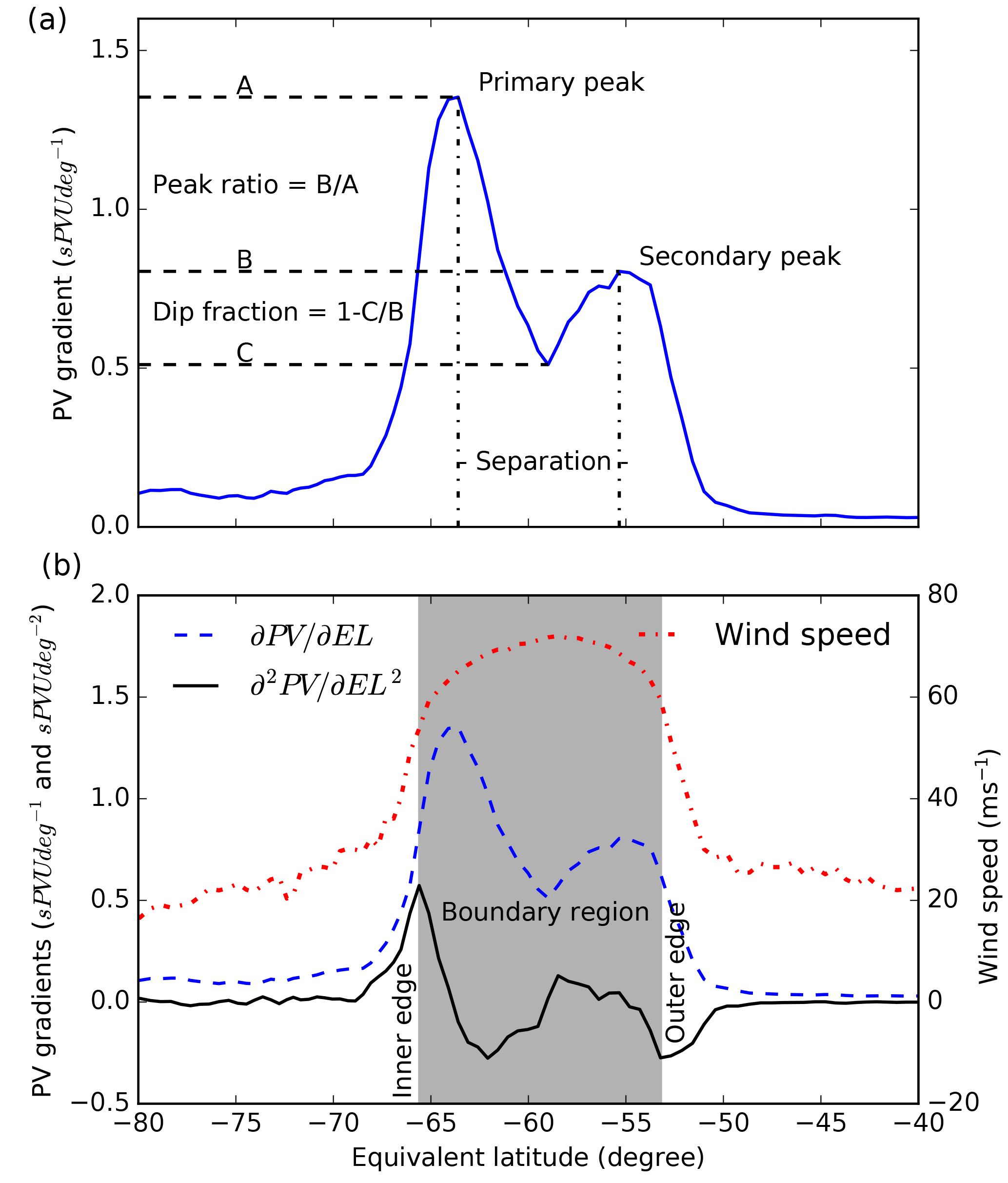
Figure 1Example of (a) the calculation of the peak ratio, dip fraction and separation from a meridional profile of PV gradient (∂PV ∕ ∂EL) and (b) the calculation of inner and outer edges of the vortex boundary region from ∂2PV ∕ ∂EL2 (sPVU ∘−2), with wind speed (m s−1) and ∂PV ∕ ∂EL (sPVU ∘−1) also shown for reference. This example is a profile at 530 K on 1 September 2007 from ERA-Interim.
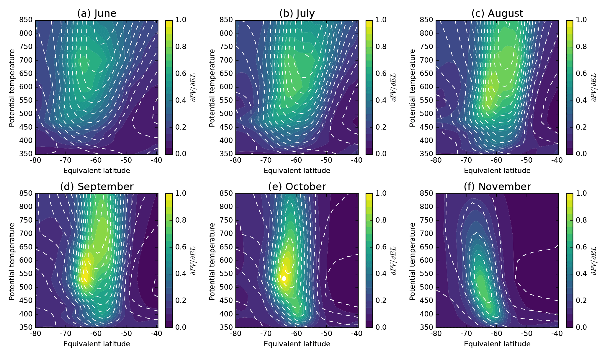
Figure 2Monthly mean PV gradient (colours; sPVU ∘−1) and wind speed (dashed lines; in 10 m s−1 steps) in 0.5∘ bins at ERA-Interim levels between 350 and 850 K, for selected months, 1979–2016.
A bifurcation index (BI) is derived using combinations of peak ratio and dip fraction that are increasingly restrictive as shown in Table 1. Single peaks are denoted as BI = 0 when the peak ratio is less than 0.5 or the dip fraction is less than 0.05. The threshold values used for determining BI were chosen to capture clearly bifurcated profiles after extensive visual inspection of PV gradients – hence only peaks with at least half the PV gradient of the main peak are considered bifurcated. In the same way, more than a 5 % dip is required between two peaks, to avoid misclassifying a “shoulder” on the main peak or noise in the PV gradient as a second peak. The two thresholds increase at the same time so that strong bifurcation requires both a similarly sized secondary peak and a very clear dip between them. Without a strong dip, a second peak of similar magnitude more likely represents a wide area of strong PV gradient rather than a distinct peak in its own right. For this reason, the dip fraction has a stronger influence on BI than peak ratio. The analysed values of dip fraction closely follow the threshold values used to define BI, whereas large peak ratios occur in profiles assessed with both small and moderate BI (not shown). Profiles assessed with small to moderate BI can range from two closely matched peaks with only a small interstitial dip to a much smaller secondary peak on the shoulder of the primary peak. Two choices of separation (2 and 5∘) were analysed for all results. Apart from the expected increase in the fraction of bifurcated profiles detected and smaller average BI for the 2∘ separation, the results do not change substantially. The more restrictive 5∘ separation is used hereafter to highlight the structure of moderate to strong bifurcation.
Table 1Threshold values of peak ratio and dip fraction used to define the bifurcation index (BI).
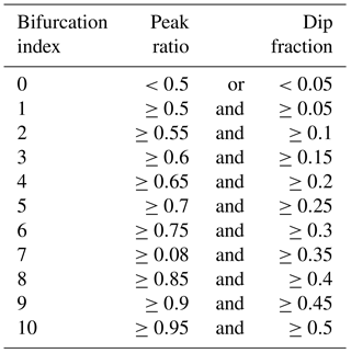
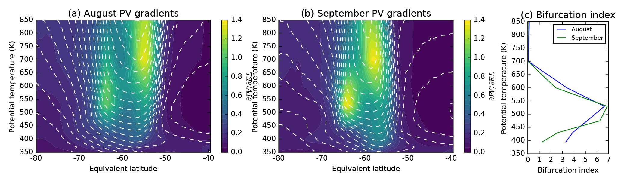
Figure 3Monthly mean PV gradient (colours; sPVU ∘−1) and wind speed (dashed lines; in 10 m s−1 steps) in 0.5∘ bins during (a) August and (b) September 2007 at ERA-Interim levels between 350 and 850 K. Also shown is (c) mean BI at each level for each month.
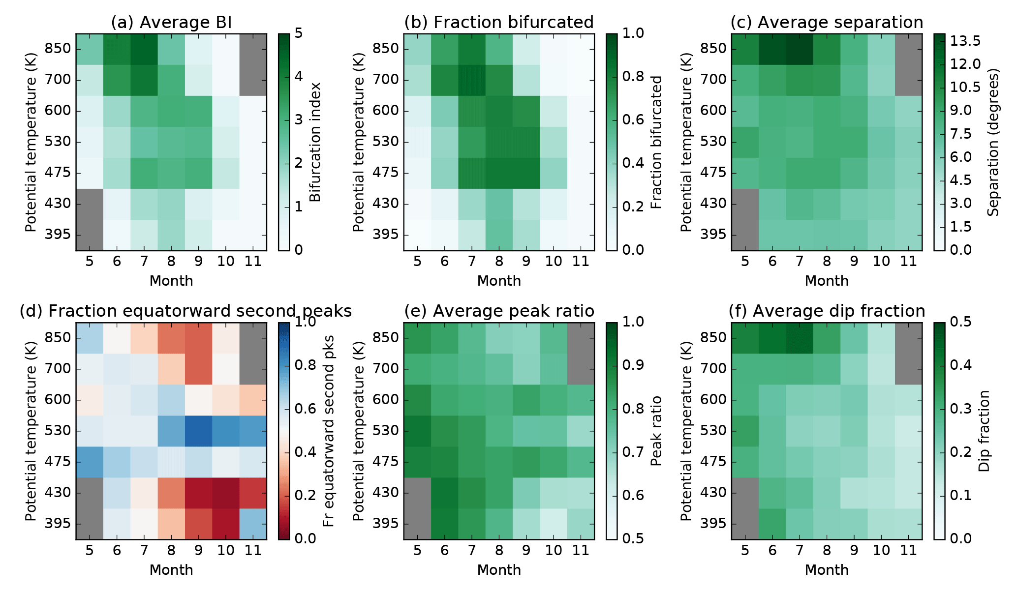
Figure 4Climatological structure and seasonal evolution of bifurcation metrics derived at ERA-Interim levels between 395 and 850 K, 1979–2016. Months/levels with less than 1 % of bifurcated profiles are shaded in grey.
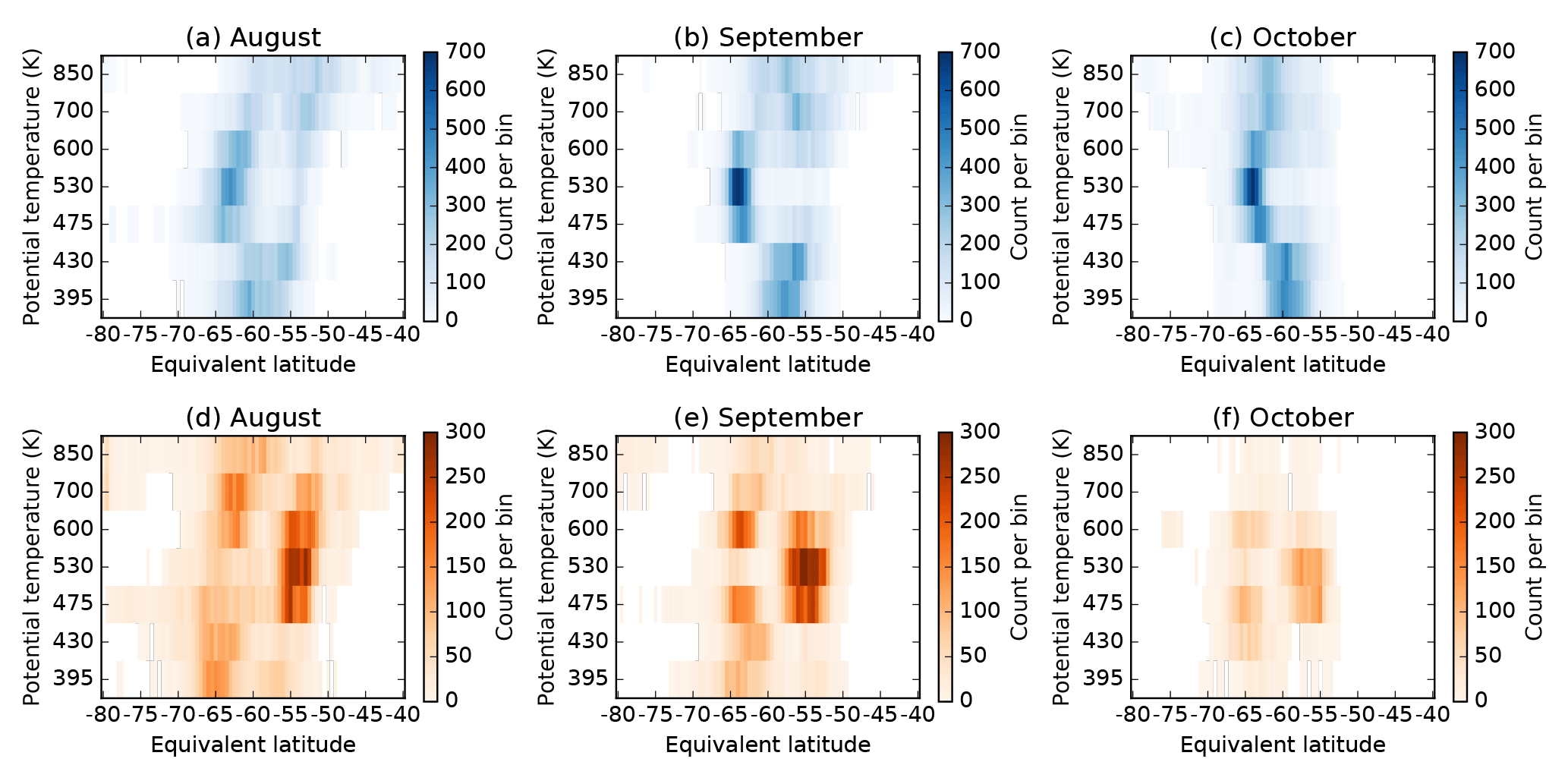
Figure 5Locations of (a–c) primary and (d–f) secondary peaks in PV gradient at ERA-Interim levels between 395 and 850 K, 1979–2016. Peaks are selected using a minimum separation of 5∘ and the colour scale shows the number of times that peaks occurred in each 0.5∘ bin.
The inner and outer edges of the vortex boundary region were calculated following Nash (1996); the inner and outer edges are evaluated as the local maximum and minimum in the second derivative of PV with respect to EL around the location of the peak in PV gradient, respectively (Fig. 1b). Note that the sign of the second derivative is opposite to the description in Nash et al. (1996) because of the negative sign convention for EL in the Southern Hemisphere. For bifurcated profiles, we nuance the Nash et al. (1996) definition by evaluating the inner edge around the poleward peak and outer edge around the equatorward peak.
3.1 Structure of meridional PV gradients in ERA-Interim
Figure 2 shows the climatological mean (1979–2016) structure of PV gradients across the polar vortex during the winter and spring. Large PV gradients generally align with the region of enhanced wind speed, which is largest at high levels during mid-winter. In August and September, PV gradients intensify in concert with the region of strong wind speed becoming predominately confined to latitudes poleward of −50∘. While increased climatological PV gradients occur over a broad region, at lower levels these are nearer the poleward edge of the wind speed jet, while at higher levels these are nearer the equatorward edge of the jet (Fig. 2c, d). As spring progresses, the vortex barrier region narrows and by the end of October only a narrow region of elevated PV gradient remains.
Considering individual years, the bifurcation of PV gradients with respect to EL becomes more apparent. The characteristic evolution of the bifurcated structure is clearly illustrated during the year 2007 (Fig. 3). The PV gradient displays two distinct peaks – one aligned with the transition to steep wind speed gradients on the equatorward side of the jet and a second peak in a similar position on the poleward flank of the jet. Between these peaks, near the region at the maximum wind speed at mid-levels, are notably reduced PV gradients. The bifurcation of PV gradients is not mirrored in the wind speed, which displays only a single broad region of maximum wind speed. Moderate to high BI occurs at mid-levels during winter and intensifies at 475 K during September (Fig. 3c).
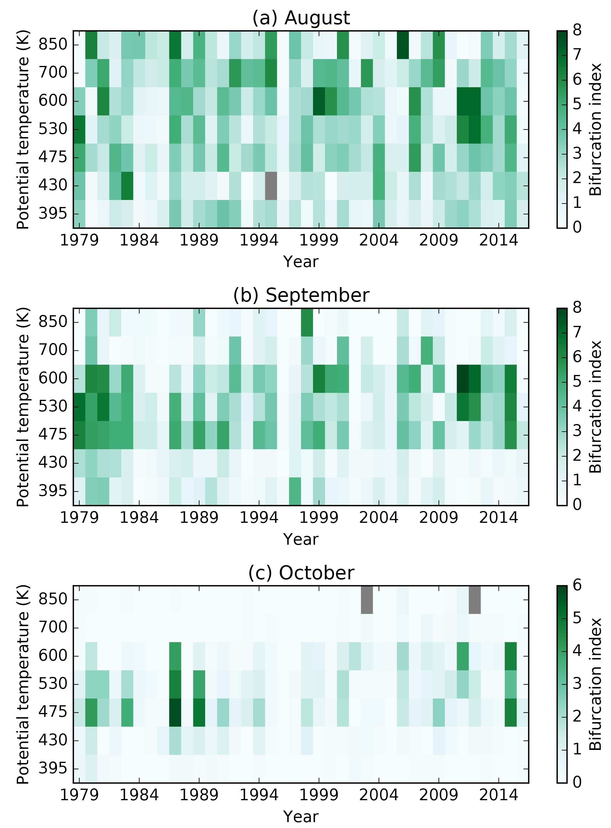
Figure 6Time series of monthly average BI at ERA-Interim levels between 395 and 850 K, 1979–2016. Grey colours indicate months with greater than 50 % of profiles that do not meet the minimum wind speed and PV gradient criteria.
3.2 Bifurcation metrics
Generally, the magnitude of BI and the frequency of bifurcation increases during the winter to peak in July or August (Fig. 4a), then decreases during spring. Low BI during October and November indicates that the vortex barrier has only a single peak, or is weakly bifurcated. At mid-levels (475 to 600 K), elevated BI remains through September, and, to a lesser extent, October. During September, the barrier is more often than not bifurcated at these levels (Fig. 4b). At all levels, the average separation between primary and secondary peaks decreases through the season from around 10∘ in June to around 5∘ in October (Fig. 4c). During the winter, there is only a slight tendency for secondary peaks to occur equatorward of primary peaks (Fig. 4d). From August onwards a more defined spatial structure develops; at mid-levels the secondary peak is most often equatorward of the primary peak. At other levels the secondary peak is more often poleward of the primary peak, though secondary peaks at these levels are not as common or strong as at mid-levels. During September, maximum values of peak ratio occur at 475 and 600 K, indicating that two peaks with similar magnitude occur frequently at these levels (Fig. 4e). The general decline in dip fraction over the season mirrors the decline in BI, showing its strong influence on BI (Fig. 4f).
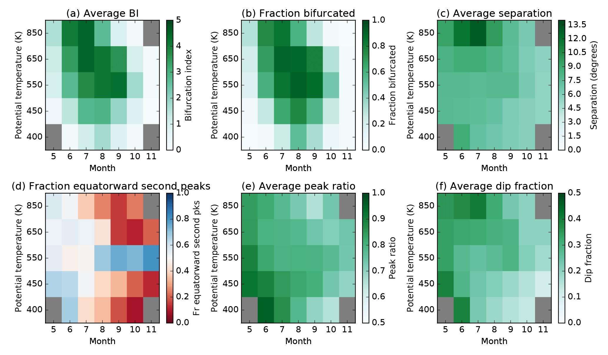
Figure 7Climatological structure and seasonal evolution of bifurcation metrics at CFSR levels between 400 and 850 K, 1979–2016. Months/levels with less than 1 % of bifurcated profiles are shaded in grey.

Figure 8Locations of (a–c) primary and (d–f) secondary peaks in PV gradient at CFSR levels between 400 and 850 K, 1979–2016. Peaks are selected using a minimum separation of 5∘ and the colour scale shows the number of times that peaks occurred in each 0.5∘ bin.
3.3 Location of primary and secondary peaks
The locations of primary and secondary peaks in PV gradient have a well-defined structure during late winter and early spring. At mid-levels (475 to 600 K), peaks in PV gradient occur in two preferred locations centred around −63 and −55∘ (Fig. 5), with primary peaks being most often in the poleward location, and secondary peaks in the equatorward location. At 700 and 850 K, the locations of primary peaks are spread across a wider range of latitude bins, especially in August. At lower levels (395 to 430 K), primary peaks are more tightly clustered around −60∘ and secondary peaks tend to be to poleward of primary peaks.
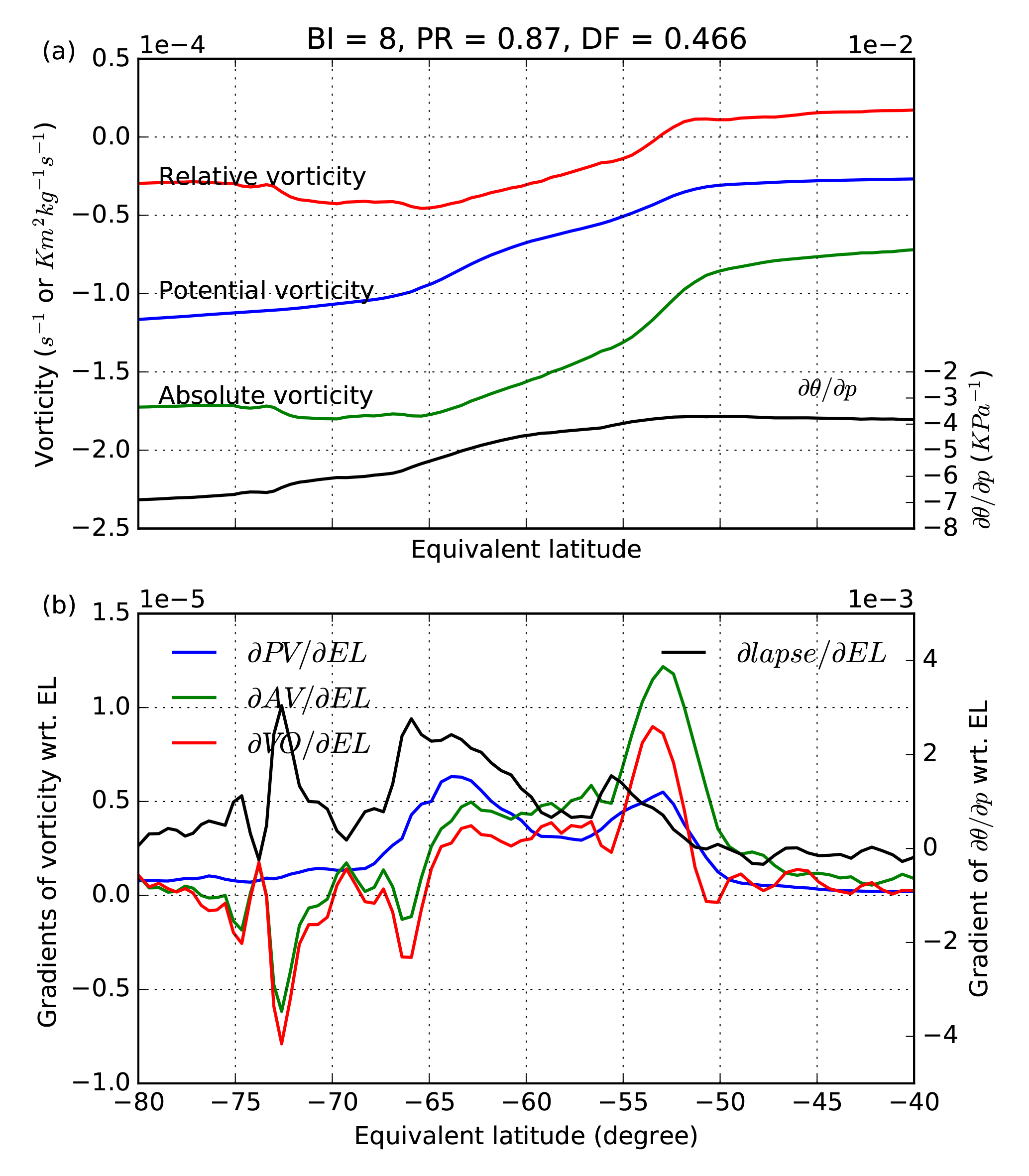
Figure 9Example meridional profile of (a) absolute (AV; green line; s−1), relative vorticity (VO; red line; s−1), and PV (blue line; K m2 kg−1 s−1) on the left axis and static stability (black line; K Pa−1) on the right axis, and (b) gradients with respect to EL (∂PV ∕ ∂EL (sPVU ∘−1)). All lines are averages at EL calculated from PV. This example is from 530 K on 1 September 2011 in ERA-Interim.
3.4 Interannual variability in bifurcation
Large interannual variations in BI display some coherence across multiple levels (Fig. 6). For example, during August, when bifurcation is common, anomalously low BI occurs simultaneously over multiple levels in a given year (e.g. 1996, 2005). During September, vertically coherent interannual variations in BI occur at mid-levels, with anomalies in BI that extend through multiple levels and weak BI above and below. During October, these anomalies persist in some years and are largely confined to 475 to 600 K. In November, the single-wall barrier predominates and bifurcation (monthly average BI >0.75) is only seen in two years (1987 at 475 and 530 K, and 2015 at 600 K).

Figure 10Gradients of PV, absolute vorticity and static stability with respect to EL for composites of years with elevated BI in selected months (a–c) July (1983, 1986, 1989, 1991, 2005), (d–f) August (1979, 2007, 2011, 2012, 2015) and (g–i) September (1980, 1981, 2011, 2012, 2015). See text for further explanation of method used to select years.
4.1 Comparison with CFSR
Average BI calculated from CFSR shows a very similar structure to that observed in ERA-Interim (Fig. 7). Bifurcation generally decreases during the spring, but remains strong at 550 and 650 K. The tendency for secondary peaks to occur equatorward of primary peaks is largely restricted to the 550 K layer, with 650 and 450 K layers displaying similar structure to those at 700 and 430 K in ERA-Interim, respectively. The average locations of primary and secondary peaks are similar, with the primary peaks at 550 K being most often in the poleward position (−63∘) during September (Fig. 8). At 650 and 450 K, primary peaks are most often situated at an equatorward location (around −55 to −58∘). The occurrence of bifurcation in a second reanalyses gives us confidence that the patterns observed are real phenomena and not artefacts of the production of a particular reanalysis data set.
4.2 Impacts of bifurcated PV gradients
The bifurcation of PV gradients across the Southern Hemisphere polar vortex represents a weakening in the rapid meridional decrease in PV that occurs across the vortex barrier. Even though PV gradients weaken between the poleward and equatorward peaks, they are still substantially larger than those in the mid-latitudes or the vortex interior. To examine the cause of bifurcation in PV gradients, we decomposed PV into its two components, absolute vorticity and static stability ( (K Pa−1)), then calculated gradients of these components with respect to EL. Absolute vorticity was calculated from relative vorticity fields downloaded from the ECMWF online archive and latitude at each grid point. Static stability was back-calculated from PV and absolute vorticity at each grid point using the equation for Ertel PV.
The gradients of vorticity and static stability at 530 K (Fig. 9) reveal the most rapid decreases in PV occur at the points where relative (and absolute) vorticity also display the most rapid decrease – in the transition from the positive vorticity associated with increasing wind speed on the outer flank of the vortex, and to the large negative vorticity associated with decreasing wind speed on the inner flank of the vortex. In addition, the gradient of static stability is greater on the inside flank of the vortex. Thus, bifurcation of PV gradients appears to be caused by the separation of two distinct zones of rapidly decreasing relative vorticity in concert with stronger gradients of static stability on the inner boundary of the vortex. During periods when the barrier is narrow, the two zones of enhanced vorticity gradient coalesce and only a single peak in PV gradient remains.
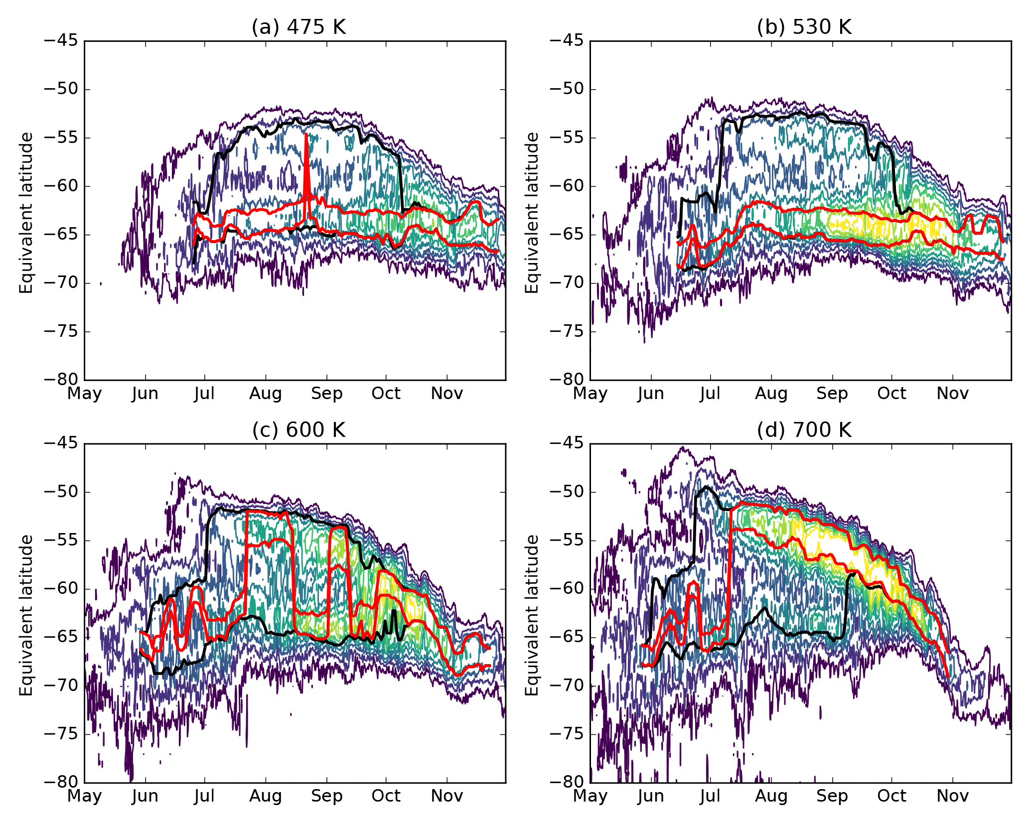
Figure 11Example showing evolution of PV gradient (coloured contours) and 7-day running average of inner and outer edges diagnosed using (red) the Nash et al. (1996) algorithm or (black) the BI algorithm presented here, during 2007 for four ERA-Interim heights. Where the black line is not visible, it is in the same position as the red line. Contours of PV gradient are given in 0.15 sPVU steps from 0.3 to 1.5 sPVU.
To extend this analysis further, we construct latitude–height composites of gradients in each component; for 1 July from 5 years with strong bifurcation at upper levels (700 and 800 K) and for 1 August and 1 September from 5 years with strong bifurcation at mid-levels (475 to 600 K). The composite analysis (Fig. 10) reinforces that bifurcation of PV gradients during August and September is associated with elevated vorticity gradients in two locations along with increased static stability gradients at the poleward location. A clear distinction in the location of maximum vorticity gradients is seen during bifurcation at mid-levels during August and September. During years with strong bifurcation at upper levels during July, the location of maximum absolute vorticity and pattern of static stability is less clear, suggesting that the location of bifurcated peaks is more dispersed, and/or the mechanism causing bifurcation at upper levels is more complex.

Figure 12Location of inner (cyan) and outer (yellow) edges of the vortex boundary region at ERA-Interim levels between 395 and 850 K, 1979–2016, defined using (a–c) the criteria of Nash et al. (1996) and (d–f) accounting for secondary peaks in PV gradient using the bifurcation algorithm presented here. The intensity of cyan and yellow represents the frequency of inner and outer boundaries in each 0.5∘ bin, respectively, with green colours indicating a mix of both inner and outer boundaries at different times. The frequency per bin is scaled with respect to a maximum count of 600 per bin.
The weakening of PV gradients within the vortex barrier during periods of bifurcation may increase mixing within the vortex boundary region, while still reducing the transport of material through the barrier as a whole. This could lead to more complex variations in trace gas concentrations across the barrier. With a single (narrower) barrier, there is less efficient mixing of air and steeper gradients in trace gas concentrations within the vortex barrier region would be expected.
Increased PV gradients observed at mid-levels during spring, on the inner flank of the vortex barrier (Fig. 5b), align with the outer limits of regions of enhanced ozone loss (Lee et al., 2001; Bodeker et al., 2002). This provides motivation for updated analyses of trends in vortex attributes, such as BI, to provide context for recent reports of trends in ozone concentrations observed during September (e.g. Solomon et al., 2016). Further work should investigate the dynamical links between ozone loss and PV gradients on the inner boundary of the vortex at mid-levels.
4.3 Redefining a vortex barrier region
If a single vortex “edge” is defined according to Nash et al. (1996), bifurcation can lead to spurious changes in the location of the vortex boundary region over time. In cases where the PV gradient has two peaks of similar magnitude, the location of the “edge” will flip-flop from one location to the other over the course of a few days, while clearly the vortex has not rapidly changed in size (Fig. 11). This challenges interpretations of the vortex “edge” that define a single location at the maximum PV gradient. By using the bifurcation algorithm described above to detect secondary peaks in the PV gradient, a more realistic and robust analysis of the location of the vortex barrier is made possible.
The Nash et al. (1996) definition of the vortex boundary region is also challenged by the bifurcated structure. The vortex boundary cannot be simply thought of as the region between the local maximum and local minimum in the second derivative of PV with respect to EL around the location of the primary peak in PV gradient. The presence of secondary peaks in PV gradient inside or outside the primary peak highlights that the region of limited mixing is, in fact, much wider than that analysed only around the primary peak.
When the bifurcation is taken into account, the width of the vortex boundary region becomes much larger than that analysed with the Nash et al. (1996) definition (Fig. 12). During August and September, a clear separation between inner and outer edges becomes apparent at mid-levels. The inner edge is predominately around −65∘, with the outer edge at around −52 to −54∘. At times, the outer edge is poleward of −60∘, but the inner edge is rarely equatorward of −60∘. At lower levels the boundary region is usually confined to a small area around the primary peak at −60∘, while at higher levels the location and width of the boundary region are much more variable. As spring progresses the boundary region coalesces at all levels.
This study suggests that there is a need to redefine the location of the vortex barrier as a boundary region in which mixing is reduced below some critical threshold, rather than as a single edge. This definition would demarcate only the inner and outer edges of the vortex boundary region, and would not be dependent on defining a single location for the vortex edge. If a single EL or PV value is needed to demarcate the vortex, then the average EL of the boundary region could still be calculated, but this value would be more robust against bifurcation than a single edge. The extension of the Nash et al. (1996) methodology shown here shows promise. Defining threshold values of PV gradient may also be a useful way to define the barrier region, though a formal comparison with other metrics of isentropic mixing (e.g. effective diffusivity, Lyapunov exponents) is warranted. This comparison would allow complementary values of each metric to demarcate the inner and outer edges to be inferred.
The strength of the dynamical isolation of high-latitude air caused by the Southern Hemisphere polar vortex has been analysed using gradients of potential vorticity along equivalent latitude coordinates for seven isentropic levels between 395 and 850 K in the ERA-Interim reanalysis for the years 1979–2016. Analyses presented here show that this barrier often displays a bifurcated structure where, rather than a single barrier to meridional mixing, a double-walled barrier exists. The bifurcated structure manifests as enhanced gradients of potential vorticity at two distinct equivalent latitudes – usually the inside and outside flanks of the region with enhanced wind speed.
Metrics quantifying the bifurcated nature of the vortex barrier have been developed and their variation in space and time has been analysed. While the height–latitude structure differs from year to year, bifurcation appears to be a persistent feature of the vortex barrier region. It was found that at most isentropic levels between 395 and 850 K, bifurcation is strongest in winter and reduces dramatically during spring as the barrier becomes more defined. From August onwards, a distinct structure emerges, with stronger bifurcation at mid-levels (475 to 600 K) and a mostly single-walled barrier at other levels. During September, peaks in PV gradient show a strong preference for two locations around −63 and −55∘ and primary peaks at 530 K are most often at the poleward location. While the strength of the bifurcation at a given level evolves from month to month and does not always persist through a season, interannual variations display coherence across multiple levels in any given month. Analysis of a second reanalysis, CFSR, shows very similar patterns. The detection of secondary peaks in PV gradient permits a more realistic view of the true region of weak mixing associated with the polar vortex.
The results presented above suggest that improved understanding of cross-vortex mixing requires consideration of the polar vortex not as a single mixing barrier but as a barrier with internal structure that is likely to manifest as more complex gradients in trace gas concentrations across the vortex boundary region. More work is needed to quantify relationships between PV gradients and other metrics of mixing (effective diffusivity, Lyapunov exponents) as well as identify the interactions between the structure of PV gradients, ozone and temperature. Analyses of trends in bifurcation should also be pursued to provide context to observed trends in ozone concentrations during springtime.
The ERA-Interim data set used in this paper is available from the ECMWF online archives: http://apps.ecmwf.int/datasets. The CFSR and CFSv2 data sets are available from https://rda.ucar.edu/datasets/ds093.0/ and https://rda.ucar.edu/datasets/ds094.0/, respectively.
JC developed and performed the analyses and prepared the manuscript with contributions from all co-authors.
The authors declare that they have no conflict of interest.
This research was funded by a Royal Society of New Zealand Marsden Fund
research grant titled “The permeability of the Antarctic vortex”, contract
number BDS1401.
Edited by: Timothy J. Dunkerton
Reviewed by: Gloria Manney
Ajtic, J., Connor, B. J., Lawrence, B. N., Bodeker, G. E., Hoppel, K. W., Rosenfield, J. E., and Heuff, D. N.: Dilution of the Antarctic ozone hole into southern midlatitudes, 1998–2000, J. Geophys. Res., 109, 1–9, https://doi.org/10.1029/2003JD004500, 2004. a
Bodeker, G. E., Struthers, H., and Connor, B. J.: Dynamical containment of Antarctic ozone depletion, Geophys. Res. Lett., 29, 1098, https://doi.org/10.1029/2001gl014206, 2002. a, b, c
Butchart, N. and Remsberg, E. E.: The area of the stratospheric polar vortex as a diagnostic for tracer transport on an isentropic surface, J. Atmos. Sci., 43, 1319–1339, https://doi.org/10.1175/1520-0469(1986)043<1319:TAOTSP>2.0.CO;2, 1986. a
Dee, D. P., Uppala, S. M., Simmons, A. J., Berrisford, P., Poli, P., Kobayashi, S., Andrae, U., Balmaseda, M. A., Balsamo, G., Bauer, P., Bechtold, P., Beljaars, A. C. M., van de Berg, L., Bidlot, J., Bormann, N., Delsol, C., Dragani, R., Fuentes, M., Geer, A. J., Haimberger, L., Healy, S. B., Hersbach, H., Hólm, E. V., Isaksen, L., Kållberg, P., Köhler, M., Matricardi, M., McNally, A. P., Monge-Sanz, B. M., Morcrette, J. J., Park, B. K., Peubey, C., de Rosnay, P., Tavolato, C., Thépaut, J. N., and Vitart, F.: The ERA-Interim reanalysis: configuration and performance of the data assimilation system, Q. J. Roy. Meteorol. Soc., 137, 553–597, https://doi.org/10.1002/qj.828, 2011. a
Dunkerton and Delisi: Evolution of Potential Vorticity in the winter Stratosphere of January-February 1979, J. Geophys. Res., 91, 1199–1208, https://doi.org/10.1029/JD091iD01p01199, 1986. a
Fujiwara, M., Wright, J. S., Manney, G. L., Gray, L. J., Anstey, J., Birner, T., Davis, S., Gerber, E. P., Harvey, V. L., Hegglin, M. I., Homeyer, C. R., Knox, J. A., Krüger, K., Lambert, A., Long, C. S., Martineau, P., Molod, A., Monge-Sanz, B. M., Santee, M. L., Tegtmeier, S., Chabrillat, S., Tan, D. G. H., Jackson, D. R., Polavarapu, S., Compo, G. P., Dragani, R., Ebisuzaki, W., Harada, Y., Kobayashi, C., McCarty, W., Onogi, K., Pawson, S., Simmons, A., Wargan, K., Whitaker, J. S., and Zou, C.-Z.: Introduction to the SPARC Reanalysis Intercomparison Project (S-RIP) and overview of the reanalysis systems, Atmos. Chem. Phys., 17, 1417–1452, https://doi.org/10.5194/acp-17-1417-2017, 2017. a
Garny, H., Bodeker, G. E., and Dameris, M.: Trends and variability in stratospheric mixing: 1979– 2005, Atmos. Chem. Phys., 7, 5611–5624, https://doi.org/10.5194/acp-7-5611-2007, 2007. a
Haynes, P. and Shuckburgh, E.: Effective diffusivity as a diagnostic of atmospheric transport: 1. Stratosphere, J. Geophys. Res.-Atmos., 105, 22777–22794, https://doi.org/10.1029/2000jd900093, 2000. a
Hoskins, B., McIntyre, M., and Robertson, A.: On the use and significance of isentropic potential vorticity maps, Q. J. Roy. Meteorol. Soc., 111, 877–946, https://doi.org/10.1002/qj.49711147002, 1985. a
Lait, L.: An alternative form of Potential Vorticity, J. Atmos. Sci., 51, 1754–1759, https://doi.org/10.1175/1520-0469(1994)051<1754:AAFFPV>2.0.CO;2, 1994. a, b
Lawrence, Z. D. and Manney, G. L.: Characterizing Stratospheric Polar Vortex Variability With Computer Vision Techniques, J. Geophys. Res.-Atmos., 123, 1510–1535, https://doi.org/10.1002/2017jd027556, 2018. a
Lee, A., Roscoe, H., Jones, A., Haynes, P., Shuckburgh, E., Morrey, M., and Pumphrey, H.: The impact of the mixing properties within the Antarctic stratospheric vortex on ozone loss in spring, J. Geophys. Res., 106, 3203–3211, https://doi.org/10.1029/2000JD900398, 2001. a
Manney, G. L. and Lawrence, Z. D.: The major stratospheric final warming in 2016: dispersal of vortex air and termination of Arctic chemical ozone loss, Atmos. Chem. Phys., 16, 15371–15396, https://doi.org/10.5194/acp-16-15371-2016, 2016. a, b, c, d
Manney, G. L., Sabutis, J. L., Allen, D. R., Lahoz, W. A., Scaife, A. A., Randall, C. E., Pawson, S., Naujokat, B., and Swinbank, R.: Simulations of Dynamics and Transport during the September 2002 Antarctic Major Warming, J. Atmos. Sci., 62, 690–707, https://doi.org/10.1175/JAS-3313.1, 2005. a
Manney, G. L., Daffer, W. H., Zawodny, J. M., Bernath, P. F., Hoppel, K. W., Walker, K. A., Knosp, B. W., Boone, C., Remsberg, E. E., Santee, M. L., Harvey, V. L., Pawson, S., Jackson, D. R., Deaver, L., McElroy, C. T., McLinden, C. A., Drummond, J. R., Pumphrey, H. C., Lambert, A., Schwartz, M. J., Froidevaux, L., McLeod, S., Takacs, L. L., Suarez, M. J., Trepte, C. R., Cuddy, D. C., Livesey, N. J., Harwood, R. S., and Waters, J. W.: Solar occultation satellite data and derived meteorological products: Sampling issues and comparisons with Aura Microwave Limb Sounder, J. Geophys. Res., 112, https://doi.org/10.1029/2007jd008709, 2007. a
McDonald, A. J. and Smith, M.: A technique to identify vortex air using carbon monoxide observations, J. Geophys. Res.-Atmos., 118, 12719–12733, https://doi.org/10.1002/2012jd019257, 2013. a
Nash, E. R., Newman, P. A., Rosenfield, J. E., and Schoeberl, M. R.: An objective determination of the polar vortex using Ertel's potential vorticity, J. Geophys. Res.-Atmos., 101, 9471–9478, https://doi.org/10.1029/96jd00066, 1996. a, b, c, d, e, f, g, h, i, j, k
Paparella, F., Babiano, A., Basdevant, C., Provenzale, A., and Tanga, P.: A Lagrangian study of the Antarctic polar vortex, J. Geophys. Res.-Atmos., 102, 6765–6773, https://doi.org/10.1029/96jd03377, 1997. a, b
Plumb, R. and Ko, M.: Interrelationships between mixing ratios of long-lived stratospheric constituents, J. Geophys. Res., 97, 10145–10156, https://doi.org/10.1029/92JD00450, 1992. a
Rummukainen, M., Knudsen, B., and von der Gathen, P.: Dynamical diagnostics of the edges of the polar vortices, Ann. Geophys., 12, 1114–1118, 1994. a
Saha, S., Moorthi, S., Pan, H.-L., Wu, X., Wang, J., Nadiga, S., Tripp, P., Kistler, R., Woollen, J., Behringer, D., Liu, H., Stokes, D., Grumbine, R., Gayno, G., Wang, J., Hou, Y.-T., Chuang, H.-Y., Juang, H.-M. H., Sela, J., Iredell, M., Treadon, R., Kleist, D., Van Delst, P., Keyser, D., Derber, J., Ek, M., Meng, J., Wei, H., Yang, R., Lord, S., Van Den Dool, H., Kumar, A., Wang, W., Long, C., Chelliah, M., Xue, Y., Huang, B., Schemm, J.-K., Ebisuzaki, W., Lin, R., Xie, P., Chen, M., Zhou, S., Higgins, W., Zou, C.-Z., Liu, Q., Chen, Y., Han, Y., Cucurull, L., Reynolds, R. W., Rutledge, G., and Goldberg, M.: The NCEP Climate Forecast System Reanalysis, Bulletin of the Am. Meteorol. Soc., 91, 1015–1057, https://doi.org/10.1175/2010bams3001.1, 2010. a
Saha, S., Moorthi, S., Wu, X., Wang, J., Nadiga, S., Tripp, P., Behringer, D., Hou, Y.-T., Chuang, H.-y., Iredell, M., Ek, M., Meng, J., Yang, R., Mendez, M. P., van den Dool, H., Zhang, Q., Wang, W., Chen, M., and Becker, E.: The NCEP Climate Forecast System Version 2, J. Climate, 27, 2185–2208, https://doi.org/10.1175/jcli-d-12-00823.1, 2014. a, b
Schoeberl, M. R. and Newman, P. A.: A multiple-level trajectory analysis of vortex filaments, J. Geophys. Res.-Atmos., 100, 25801–25815, https://doi.org/10.1029/95JD02414, 1995. a
Schoeberl, M. R., Lait, L. R., Newman, P. A., and Rosenfield, J. E.: The structure of the polar vortex, J. Geophys. Res.-Atmos., 97, 7859–7882, https://doi.org/10.1029/91JD02168, 1992. a
Serra, M., Sathe, P., Beron-Vera, F., and Haller, G.: Uncovering the Edge of the Polar Vortex, J. Atmos. Sci., 74, 3871–3885, https://doi.org/10.1175/jas-d-17-0052.1, 2017. a
Smith, M. L. and McDonald, A. J.: A quantitative measure of polar vortex strength using the functionM, J. Geophys. Res.-Atmos., 119, 5966–5985, https://doi.org/10.1002/2013jd020572, 2014. a
Solomon, S.: Stratospheric ozone depletion: a review of concepts and history, Rev. Geophys., 37, 275–316, https://doi.org/10.1029/1999RG900008, 1999. a
Solomon, S., Ivy, D. J., Kinnison, D., Mills, M. J., Neely, R. R., and Schmidt, A.: Emergence of healing in the Antarctic ozone layer, Science, 353, 269–274, https://doi.org/10.1126/science.aae0061, 2016. a
Struthers, H., Bodeker, G. E., Austin, J., Bekki, S., Cionni, I., Dameris, M., Giorgetta, M. A., Grewe, V., Lefèvre, F., Lott, F., Manzini, E., Peter, T., Rozanov, E., and Schraner, M.: The simulation of the Antarctic ozone hole by chemistry-climate models, Atmos. Chem. Phys., 9, 6363–6376, https://doi.org/10.5194/acp-9-6363-2009, 2009. a
Waugh, D. W. and Randel, W.: Climatology of Arctic and Antarctic Polar Vortices Using Elliptical Diagnostics, J. Atmos. Sci., 56, 1594–1613, https://doi.org/10.1175/1520-0469(1999)056<1594:COAAAP>2.0.CO;2, 1999. a, b