Climatological study of the Boundary-layer air Stagnation Index for China and its relationship with air pollution

The Air Stagnation Index (ASI) is a vital meteorological measure of the atmosphere's ability to dilute air pollutants. The original metric adopted by the US National Climatic Data Center (NCDC) is found to be not very suitable for China, because the decoupling between the upper and lower atmospheric layers results in a weak link between the near-surface air pollution and upper-air wind speed. Therefore, a new threshold for the ASI–Boundary-layer air Stagnation Index (BSI) is proposed, consisting of daily maximal ventilation in the atmospheric boundary layer, precipitation, and real latent instability. In the present study, the climatological features of the BSI are investigated. It shows that the spatial distribution of the BSI is similar to the ASI; that is, annual mean stagnations occur most often in the northwestern and southwestern basins, i.e., the Xinjiang and Sichuan basins (more than 180 days), and least over plateaus, i.e., the Qinghai–Tibet and Yunnan plateaus (less than 40 days). However, the seasonal cycle of the BSI is changed. Stagnation days under the new metric are observed to be maximal in winter and minimal in summer, which is positively correlated with the air pollution index (API) during 2000–2012. The correlations between the BSI and the concentration of fine particulate matter (PM_2.5) during January 2013 and November to December in 2015–2017 of Beijing are also investigated. It shows that the BSI matches the day-by-day variation of PM_2.5 concentration very well and is able to catch the haze episodes.

1 Introduction

Air pollution has attracted considerable national and local attention and become one of the top concerns in China (e.g., Chan and Yao, 2008; Guo et al., 2014; Huang et al., 2014; Peng et al., 2016). It is also a worldwide problem, shared by the US, Europe, India, etc. (e.g., Lelieveld et al., 2015; van Donkelaar et al., 2010; Lu et al., 2011). The initiation and persistence of air pollution episodes involve complex processes, including direct emissions of air pollutants, and secondary formation by atmospheric chemical reactions. Meteorological background is also significant for its ability to affect the accumulation and removal or dispersion of air pollutants (e.g., Tai et al., 2010; Chen and Wang, 2015; Dawson et al., 2014). A substantial number of studies have been carried out on the abnormal meteorological conditions during haze events. They suggested that a persistent or slow moving anti-cyclone synoptic system inclines to form a haze episode (Ye et al., 2016; Leibensperger et al., 2008; Liu et al., 2013; Yin et al., 2017). Besides the driving force from a synoptic scale, some local meteorological conditions are also favorable for heavy air pollution. Low atmospheric boundary layer (ABL) height can act as a lid to confine the vertical mixing of air pollutants (Zhang et al., 2010; Ji et al., 2012; Bressi et al., 2013). Light winds lack the ability to disperse air pollutants or transport them far away (Fu et al., 2014; Rigby and Toumi, 2008; Tai et al., 2010), and those pollutants blown by winds could directly contaminate the downwind zone (Wehner and Wiedensohler, 2003; Elminir, 2005). In addition, high relative humidity usually results in low visibilities through aerosol hygroscopic growth (Chen et al., 2012; Quan et al., 2011). Studies have shown that haze pollution in China occurs more frequently over recent decades, especially that in the eastern region (Wang and Chen, 2016; Pei et al., 2018). Apart from increased emissions of pollutants, climate change also plays an important role in air pollution intensification. Fewer cyclone activities and weakening East Asian winter monsoons (Pei et al., 2018; Yin et al., 2017) resulting from the decline of Arctic sea ice extent (Deser et al., 2010; Wang and Chen, 2016) and an expanded tropical belt (Seidel et al., 2008) are believed to bring about a more stable atmosphere in eastern China and cause more haze days (Wang et al., 2015). Hence, the analysis of meteorological background related to air pollution is of great importance.

Researchers have developed many indexes comprised of different meteorological variables to describe the ability of transport and dispersion of the atmosphere. For example, Cai et al. (2017) constructed a haze weather index with 500 and 850 hPa wind speeds and temperature anomalies between 850 and 250 hPa. Han et al. (2017) proposed an air environment carrying capacity index including air pollutant concentration, precipitation, and ventilation coefficient. Among these indexes, the Air Stagnation Index (ASI), consisting of upper- and lower-air winds and precipitation, has been in use till today. The US National Climatic Data Center (NCDC) has monitored monthly air stagnation days for the United States since 1973 to indicate the temporal buildup of ozone in the lower atmosphere (http://www.ncdc.noaa.gov/societal-impacts/air-stagnation/, last access: 30 May 2018). A given day is considered stagnant when the 10 m wind speed is less than 3.2 m s⁻¹ (i.e., near-surface wind is insufficient to dilute air pollutants), 500 hPa wind speed less than 13 m s⁻¹ (i.e., lingering anti-cyclones, indicating weak vertical mixing), and no precipitation occurs (i.e., no rain to wash out the pollutants) (Korshover, 1967; Korshover and Angell, 1982; Wang and Angell, 1999; Leung and Gustafson, 2005; Horton et al., 2014). Perturbation studies have proven that air stagnation positively correlates with ozone and particulate matter concentrations (e.g., Liao et al., 2006; Jacob and Winner, 2009).

Huang et al. (2017) followed the NCDC's metric of air stagnation and investigated the climatological mean features of it for China. It was found that the spatial distribution of annual mean stagnations is in good agreement with that of the air pollution index (API). Basins in Xinjiang and Sichuan provinces are reported to experience heavy air pollution most often (Wang et al., 2011, 2012; Chen and Xie, 2012; Li et al., 2015), and according to Huang et al. (2017), these two basins were identified as regions with the most frequent stagnation occurrence (50 % days per year). However, the seasonal variation pattern of air stagnation barely correlated with that of the API. Stagnations happen most frequently in summer and least in winter, whereas the API has the opposite seasonal pattern (Li et al., 2014). Why does the NCDC criterion fail to represent it? As the mid-tropospheric wind is the main driving force of air stagnations (Huang et al., 2017), we analyzed the 500 hPa wind speed on the most polluted days of Beijing when their API ranks in the 90th percentile or higher in the autumn and winter seasons of each year during 2000–2012 (Fig. 1). It is found that on 75 % of the most polluted days, the 500 hPa wind speed is stronger than 13 m s⁻¹. It suggests that air pollution does not necessarily link with weak upper-air wind speed, and thus weak 500 hPa wind speed is not an appropriate indicator of pollution occurrence.

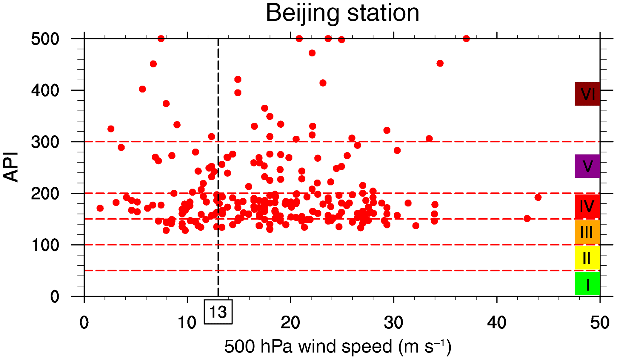
Figure 1 The relationship between the air pollution index (API) and 500 hPa wind speeds on most polluted days (i.e., days when the API ranks in the 90th percentile or higher) in the boreal winter half-year (October–March) during 2000–2012 of Beijing station. Air pollution is classified into six levels (I–VI), which mean excellent, good, lightly polluted, moderately polluted, heavily polluted, and severely polluted conditions, respectively.

In order to address this deficiency, Wang et al. (2017) tried to modify the ASI by taking 10 m wind speed, ABL height, and the occurrence of precipitation into consideration. Their air stagnation threshold is determined by a fitting equation which relates to PM_2.5 concentration, 10 m wind speed, and ABL height. This equation varies with locations and changes over time. In this study, we propose a new air stagnation identification–Boundary-layer air Stagnation Index (BSI). Instead of relating this index directly to air pollution monitoring data, we put the thresholds on a meteorological basis only and hope that the BSI is more universal and robust in principle. The BSI metric retains a no-precipitation threshold to exclude wet deposition, gives upper-air wind speed, replaces 10 m wind speed with ventilation in the ABL to represent both the horizontal dilution and vertical mixing scale of the atmosphere, and takes real latent instability of the surface atmosphere into consideration. The components of the BSI are introduced one by one in the following, except the precipitation threshold.

The depth of the ABL is of much concern in air pollution studies, since it acts as the vertical mixing confinement of air pollutants, and in turn determines surface concentrations of them. The ABL depth normally shows a diurnal cycle: a minimum at night and maximum in the afternoon (Stull, 1988). This is the vertical mixing extent of air pollutants. On the other hand, the strength of horizontal dilution (i.e., transport wind speed) is also significant in atmospheric dispersion and presents a similar diurnal pattern to ABL height. For the consideration of environmental capacity, mixing layer depth (MD) and transport wind in the afternoon are of great importance since they together represent the best dilution condition during the entire day (Holzworth, 1964; Miller, 1967). Therefore, ventilation in the maximum MD (referred to as ventilation hereinafter) is adopted in the BSI as a mixture to simultaneously indicate the largest extent of horizontal dilution and vertical mixing.

MD is not a quantity of routine meteorological observation (Liu and Liang, 2010). It is usually derived from profiles of the temperature and wind speed/direction as well as humidity from a local and short-term observation project or experiment (Seibert et al., 2000). The methods used to detect or estimated MD include observation of sodar (Beyrich, 1997; Lokoshchenko, 2002), lidar (Tucker et al., 2009), ceilometers (Eresmaa et al., 2006; van der Kamp and McKendry, 2010), and wind profilers (Bianco and Wilczak, 2002). Holzworth (1964, 1967) pioneered the work to obtain long-term, large area maximum MD (MMD) information by the “parcel method”, in which MMD is interpreted as the height above ground of dry-adiabatic intersection of the maximum surface temperature during the daytime with the vertical temperature profile from morning (12:00 UTC for China) radiosonde observation. Seidel et al. (2010) compared MMD results from the parcel method along with six other methods using long-term radiosonde observations, and concluded that climatological MMD based on the parcel method is warranted for air quality studies. Their further work (Seidel et al., 2012) compared the results derived from sounding data with other climate models, and provided a comparison of the MD characteristics between North America and Europe. These two studies lay the groundwork for the global climatology of MD. Since then, the climatological characteristics of MD over regional (e.g., for the Swiss plateau by Coen et al., 2014; for the Indian sub-continent by Patil et al., 2013) or global scales have been investigated (von Engeln and Teixeira, 2013; Ao et al., 2012; Xie et al., 2011; Jordan et al., 2010).

MMD derived from the parcel method is recommended for air pollution potential evaluation. However, in the presence of clouds, it agrees well with the depth of the cloud base (Seidel et al., 2010), which is lower than the actual magnitude of the vertical mixing extent of air pollutants. In order to compensate for this deficiency, we take the thermo-dynamical parameter convective available potential energy (CAPE) into consideration, implying the energy of ascension from the base to top of the cloud (Riemann-Campe et al., 2011). CAPE denotes the potential energy available to form cumulus convection and thus serves as an instability index (Blanchard, 1998). It is a measurement of the maximum kinetic energy per unit air mass achieves by rising freely from the level of free convection (LFC) and the level of neutral buoyancy (LNB) (i.e., bottom and top of the cloud), since the virtual temperature of the buoyant parcel is higher than that of its environment (Markowski and Richardson, 2011). Holton (1992) indicated that when buoyancy is the only force of an air parcel, CAPE corresponds to the upper limit for the vertical component of the velocity, as CAPE = $w_{\max }^{\mathrm{2}}/\mathrm{2}$. However, high values of CAPE do not necessarily lead to strong convection (Williams and Renno, 1993). Its opposing parameter convective inhibition (CIN) describes the energy needed by the rising air parcel to overcome the stable layer between the surface and LFC (Markowski and Richardson, 2011; Riemann-Campe et al., 2009). CAPE stored in the atmosphere is activated if the value of CAPE is larger than that of CIN, that is, under real latent instability conditions. Therefore, climatological study of CAPE and CIN provides an insight into the strength of atmospheric convection (Monkam, 2002).

In summary, unfavorable meteorological variables are critical to the occurrence of air pollution episodes. The ASI from NCDC is designed to evaluate the air dilution capability, but is found to be inappropriate for China. So we propose a new stagnation index, the BSI, instead. Our aim in the present work is to investigate the climatological features of the BSI, as well as its components, and examine the practicability of the BSI by studying its relationship with air quality monitoring data, i.e., API data during 2000–2012, and concentrations of fine particulate matter (PM_2.5) in January 2013 of Beijing.

2 Data and methodology

2.1 Data

2.1.1 Meteorological data

Radiosonde data are used to calculate the daily ventilation. Soundings from all the international exchange stations across China (95 stations) for the 30-year period (1985–2014) were obtained from the archive of the University of Wyoming (available at http://weather.uwyo.edu/upperair/sounding.html, last access: 30 May 2018). This dataset provides twice daily (00:00 and 12:00 UTC) atmospheric soundings, including the observed temperature, geopotential height, and wind speed data at pressure levels, as well as additionally derived variables CAPE and CIN.

Surface observational data are used to identify daily maxima of surface air temperature. We extracted hourly observations of surface air temperature during 1985 to 2014 from the Integrated Surface Database (ISD), provided by the NCDC. Data are accessible from FTP (ftp://ftp.ncdc.noaa.gov/pub/data/noaa, last access: 30 May 2018). The entire ISD archive has been previously processed through quality control procedures by the NCDC, including algorithms checking for extreme values and limits, consistency between parameters, and continuity between observations. More detailed information regarding the quality control process can be found at https://www.ncdc.noaa.gov/isd (last access: 30 May 2018).

Long-term (1985–2014) daily precipitation data were collected from the China Meteorological Administration (CMA). These data are available at http://data.cma.cn/data/detail/dataCode/SURF_CLI_CHN_MUL_DAY_CES_V3.0.html (last access: 30 May 2018).

For any investigation, we limited the study to the stations where all the quantities – radiosondes, surface temperature observations, and daily precipitation data – are available together. Therefore, air stagnations of 66 stations are analyzed in this study. Figure 2 shows that these 66 stations are fairly spread all over contiguous China, except that the Qinghai–Tibet Plateau, particularly western Tibet, is not well sampled.

We conducted a general survey of the availability of valid data (radiosonde data, daily maximum temperature, and daily precipitation are valid at the same time) for each of the 66 stations (Appendix A). It shows that among these 66 stations, datasets of 62 stations are available from January 1985 to December 2014, while datasets of the other 4 stations (Wenjiang, Jinghe, Chongqing, Shanghai) cover less than 30 years. The shortest duration is 9 years at Wenjiang station. The percentage of valid data are more than 96 % of each station. In conclusion, the datasets are sufficient for us to conduct a climatological study of the BSI on a countrywide basis.

2.1.2 Air quality data

To discuss the practical applicability of the BSI, daily API data (available at http://datacenter.mep.gov.cn, last access: 30 May 2018) of four representative stations (Harbin, Urumqi, Beijing, and Chongqing) during 2000–2012 are used. In order to exclude the influences of emission variations and chemical reactions to the greatest extent, and focus on the effects of meteorological conditions, we only analyse API data on those days when the primary pollutant is PM_2.5. The concentration of PM_2.5 is also used as another good metric for air pollution. We collected 24 h averaged PM_2.5 concentrations of Beijing during November to December in 2015–2017 from the Ministry of Environmental Protection (MEP) of China. The concentrations during January 2013 are not yet accessible from the MEP, so we obtained the hourly data from the US Embassy instead. With these concentrations, we conducted case studies and examined the ability of the BSI to track day-by-day variation of air pollution.

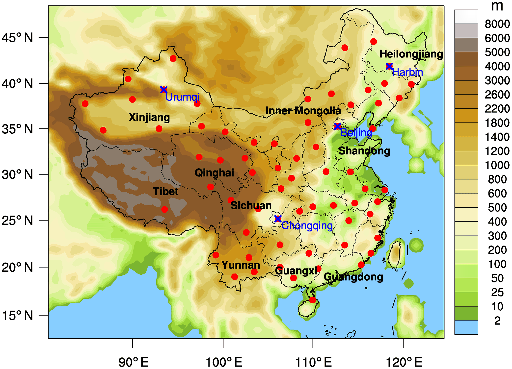
Figure 2 Topography of China and locations of 66 stations analyzed in this study. Cross marks indicate the four representative stations: Harbin, Urumqi, Beijing, and Chongqing.

2.2 Method

2.2.1 Daily MMD and ventilation

The parcel method (Holzworth, 1964) is used to calculate daily MMD. There are two steps in this calculation: (1) identify the daily maximum surface air temperature from hourly temperature data from 08:00 to 20:00 BJT (Beijing standard time; UTC+8); (2) starting from the maximal surface temperature, a dry-adiabatic line extends to intersect the temperature profile of morning sounding. Then the intersection height above ground level is MMD. Since the vertical resolution is coarse (10¹–10² m), the data of temperature from the radiosonde were interpolated linearly to height levels with 1 m vertical resolution. It is noticed that the parcel method may fail to determine the MMD sometimes when the temperature profile itself is close to a dry-adiabatic line (Lokoshchenko, 2002) or the height corresponding to the first valid value of the temperature is too high. These cases are treated as missing data and ignored.

Wind speeds at 12:00 UTC (i.e., 20:00 BJT) from radiosonde were also interpolated linearly to height levels with 1 m resolution, and ventilation is derived by integrating the wind speeds from the surface to the top of the maximum mixing layer:

$$\begin{array}{}\text{(1)}& {\displaystyle }{\displaystyle }\mathrm{vent}=\underset{\mathrm{0}}{\overset{\mathrm{MMD}}{\int }}u\left(z\right)\mathrm{d}z,\end{array}$$

where “vent” is short for ventilation, z is the elevation above the surface, and u(z) is the wind speed at z m above the ground. Ventilation is a direct measure of the dilution capacity of the atmosphere within the ABL. Higher values of ventilation indicate effective dilution.

From Eq. (1), the average value of the wind speed through the MMD, i.e., the transport wind speed (U_T), is written as

$$\begin{array}{}\text{(2)}& {\displaystyle }{\displaystyle }{U}_{\mathrm{T}}=\mathrm{vent}/\mathrm{MMD}.\end{array}$$

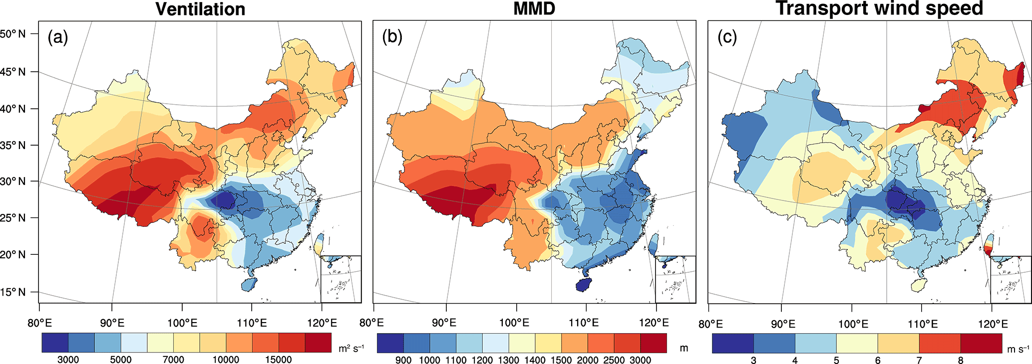
Figure 3 The spatial distribution of daily maximal ventilation (a), MMD (b), and transport wind speed (c) averaged over 30 years (1985–2014).

2.2.2 CAPE and CIN

The values of CAPE and CIN are taken directly from the sounding files provided by the University of Wyoming. Based on pseudo-adiabatic assumption, the formula for CAPE calculation (Murugavel et al., 2012) is

$$\begin{array}{}\text{(3)}& {\displaystyle }{\displaystyle }\mathrm{CAPE}=g\sum _{\mathrm{LFC}}^{\mathrm{LNB}}{\displaystyle \frac{\mathrm{\Delta }z\left(T_{\mathrm{vp}}-T_{\mathrm{ve}}\right)}{T_{\mathrm{ve}}}},\end{array}$$

where T_vp designates the virtual temperature of the lifted air parcel of the lowest 500 m of the atmosphere, T_ve is the virtual temperature of the environment, Δz is incremental depth, and g is the gravitation constant. Only values of CAPE calculated from 12:00 UTC (i.e., 20:00 BJT) profiles are considered for this analysis, representing the maximum convective potential energy of the day.

The value of CAPE is sensitive to the calculation method, such as the treatment of the freezing process (Williams and Renno, 1993; Tompkins and Craig, 1998; Frueh and Wirth, 2007). However, climatological mean features of CAPE are not sensitive to the calculation method if one particular method is applied throughout (Myoung and Nielsen-Gammon, 2010; Murugavel et al., 2012). Therefore, our results are assumed to be insensitive to the method of CAPE calculation.

CIN is calculated through

$$\begin{array}{}\text{(4)}& {\displaystyle }{\displaystyle }\mathrm{CIN}=-g\sum _{Z_{\mathrm{surface}}}^{\mathrm{LFC}}{\displaystyle \frac{\mathrm{\Delta }z\left(T_{\mathrm{vp}}-T_{\mathrm{ve}}\right)}{T_{\mathrm{ve}}}}.\end{array}$$

It should be noted that values of CIN in the following discussion all refer to the absolute values of CIN.

2.2.3 Criteria for the BSI

The BSI is designed to better describe the atmospheric dispersion capability in the ABL. A given day is considered stagnant when the value of daily maximum ventilation is less than 6000 m² s⁻¹ (Holzworth, 1972), the value of CAPE is less than that of CIN, and daily total precipitation is less than 1 mm (i.e., a dry day). The definition of an air stagnation case is retained: 4 or more consecutive air stagnant days are considered as one air stagnation case (Wang and Angell, 1999). In order to show the spatial distribution of stagnation days and cases over continental China, results of 66 stations have been interpolated in space on the 2^∘ × 2^∘ grid by cubic splines.

3 Climatology of the BSI components: ventilation, precipitation, and real latent instability

3.1 Ventilation climatology

The daily maximal ventilation condition is distributed with substantial regional heterogeneity (Fig. 3a). It is shown that ventilation might be the largest (more than 15 000 m² s⁻¹) over the Qinghai–Tibet Plateau, which is the world's highest plateau, with an average elevation exceeding 4500 m. The areas neighboring the plateau, the Yunnan Plateau and Inner Mongolian Plateau, also experience relative large ventilation (10 000–15 000 m² s⁻¹). However, the south of China, where the population and industry are dense, exhibits the most unfavorable atmospheric ventilation conditions, especially the Sichuan Basin, where the ventilation is lower than 4000 m² s⁻¹.

Figure 4 Annual cycle of ventilation, MMD, and transport wind speed of four representative stations (Harbin, Urumqi, Beijing, and Chongqing). Monthly mean values are given as horizontal bars in the middle, 25 and 75 % percentiles are shown as the boxes' lower and upper boundaries, and 10 and 90 % percentiles as lower and upper whiskers.

Figure 5 The spatial distribution of annual precipitation (a) and precipitation days (b) during 1985–2014.

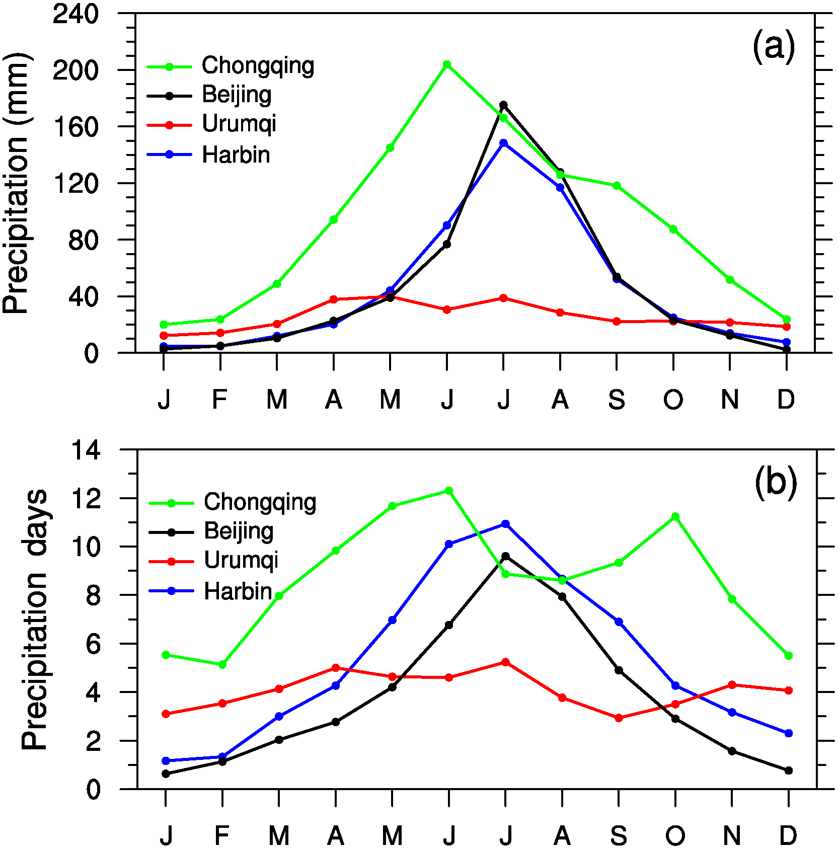
Figure 6 Annual cycle of precipitation (a) and precipitation days (b) of four representative stations (Harbin, Urumqi, Beijing, and Chongqing).

Ventilation is a combined response of both the MMD and transport wind speed. It is noticed that regions with high ventilation also experience relatively high MMD and strong transport wind, whereas regions with poor ventilation conditions also exhibit low MMD and weak transport wind (Fig. 3). First of all, large MMD (more than 2000 m) is observed over the Qinghai–Tibet–Yunnan Plateau, whereas low MMD (about 1000 m or less) is located in southeastern China (Fig. 3b). This distribution pattern is interpreted as the effect of terrain. High terrain elevation corresponds to thinner air and a lower value of aerosol optical thickness, less precipitable water vapor amount, and stronger solar radiation (Chen et al., 2014; Zhu et al., 2010), which enhance thermal convections and lead to high MMD. The results agree with the recent study of Liu et al. (2015). Secondly, the plateau is located right in the westerlies, and it can even break the jet stream into two branches surrounding the northern and southern edges of the plateau. Therefore, as Schiemann et al. (2009) revealed, the transport wind is strong (more than 6 m s⁻¹) over plateaus (Fig. 3c) because of the combined influence of westerly jet and elevated topography, and weak (less than 4 m s⁻¹) over the Xinjiang and Sichuan basins. Based on the analyses above, the results over the Tibetan Plateau are considered reasonable, although observation stations are sparse there.

Generally, most regions of China experience a good ventilation condition in spring (Fig. S1 in the Supplement). Specifically, different regions show different seasonal variation patterns. Four representative stations (Harbin, Urumqi, Beijing, and Chongqing, shown in Fig. 2 as crosses) are selected to analyze the monthly variation of ventilation, as well as the corresponding MMD and transport wind speed (Fig. 4). It is shown that patterns of the monthly variation of ventilation are different at different stations. Ventilations of Harbin and Beijing reach a peak in April, followed by a rapid fall to a low value in August. Subsequently, these values increase to a secondary peak in October and then decrease to the minima in January. Correspondingly, MMD and transport wind speed also show a bimodal distribution pattern with two peaks: one in spring and another in autumn. For North China, solar radiation is strong in summer, but significant rains and cloudy skies restrict the thermal convective processes and keep the MMD to a low value in the monsoon season. In addition, the wind speed is typically weaker in summer and stronger in winter (Frederick et al., 2012). However, the winter solar radiation is weak and constrains the development of the atmospheric boundary layer. Consequently, weak transport wind and poor ventilation are observed in both summer and winter. The seasonal behavior of ventilation conditions of Urumqi is different. The monthly mean value of ventilation presents a unimodal distribution with the mean value ranging from 788 m² s⁻¹ (January) to 15 544 m² s⁻¹ (June) through the year. The corresponding MMD and transport wind speed also show similar seasonal behavior, ranging from 334 m and 2.2 m s⁻¹ in January to 2406 m and 6.2 m s⁻¹ in June, respectively. This may be attributed to the unique local climate of northern Xinjiang, where the climate is considered semi-arid steppe (Peel et al., 2007). In Urumqi, short summer and long winter are the dominant seasons, while spring and autumn are only transitional ones (Domroes and Peng, 1988). Monthly precipitation averaged over the recent 30 years (1985–2014) ranged between 12.2 mm (January) and 39.9 mm (May), demonstrating the arid climate of Urumqi (shown later in Fig. 6). The lack of precipitation (especially in summer) may lead to a unimodal distributed MMD and ventilation condition in Urumqi. Apart from its one-peak pattern, the transport wind speed in Urumqi is weaker than that in Harbin and Beijing, owing to the block of the Qinghai–Tibet Plateau in the south. Chongqing, on the other hand, is an extreme example, where atmospheric ventilation is poor (lower than 10 000 m² s⁻¹) throughout the year. Along with this are low MMD (lower than 1500 m) and weak transport wind (weaker than 4 m s⁻¹). This natural situation may put large pressure on local air quality.

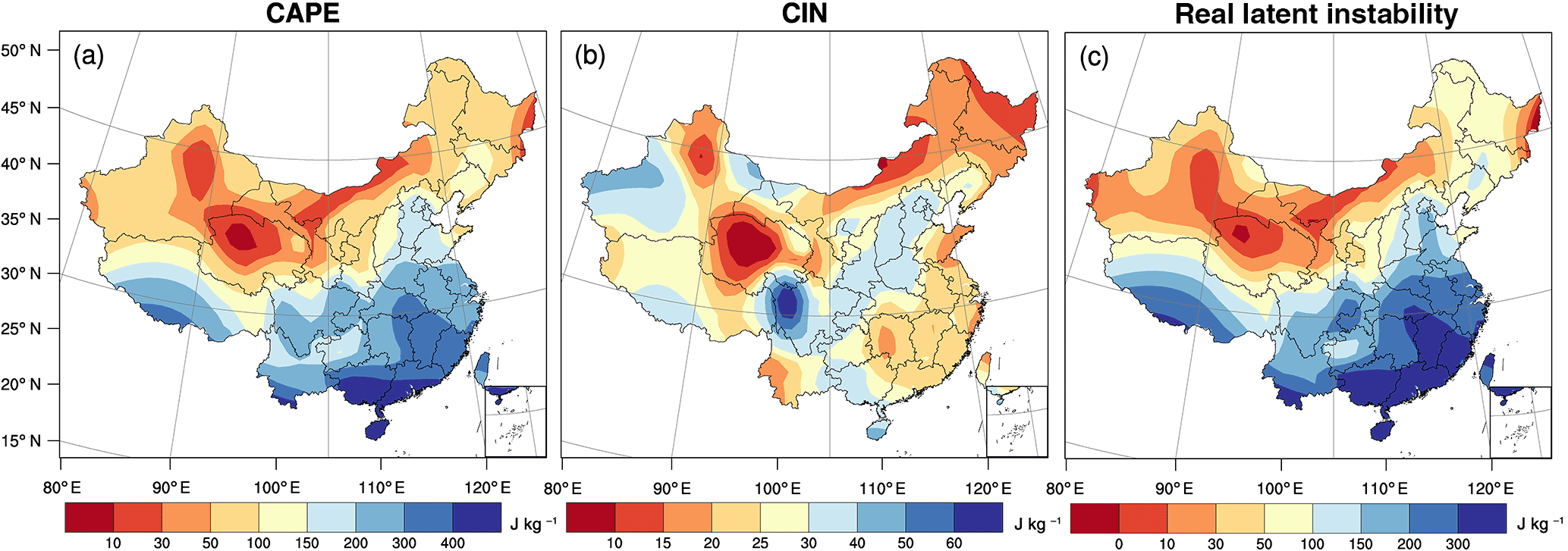
Figure 7 The spatial distribution of annual mean CAPE (a), CIN (b), and real latent instability (c) during 1985–2014.

3.2 Precipitation climatology

Another component for the BSI is precipitation, which is retained from the metric for the ASI. Figure 5 shows that the rainfall amount and rainy days are observed to be more significant over the southeast of China than inland areas due to the transport of moisture from the ocean by the summer monsoon (Fig. S2). Rainfall amount and rainy days of four representative stations (Harbin, Urumqi, Beijing, and Chongqing) are shown in Fig. 6. It is seen that generally, Chongqing experiences the largest annual rainfall amount and Urumqi the least (Fig. 6a). Seasonally, rainfall is abundant in the summer monsoon season and scarce in winter for Harbin, Beijing, and Chongqing. But for Urumqi, it maintains a low value throughout the year, illustrating the arid climate in the northwest of China. As for the rainy days, Harbin and Beijing experience most of them in the summer monsoon season, sharing the similar unimodal pattern with their monthly rainfall amount. Rainy days of Urumqi maintain a low value all the year round, the same as the pattern of its rainfall amount. However, the variation of rainy days (Fig. 6b) of Chongqing shows two distinct peaks: one is seen in May and June (about 12 days) and another in October (about 11 days). It indicates that autumn in Chongqing is characterized by moderate rain with more frequency.

3.3 CAPE and CIN climatology

Apart from the actual rainfall to wash out air pollutants, CAPE is also important since it relates to convection initiations and thermodynamic speed limits (Markowski and Richardson, 2011). Larger values of CAPE with CIN deducted (referred to as CAPE_CIN hereinafter) mean a higher probability in the destabilization of the atmosphere and genesis of stronger wet convection.

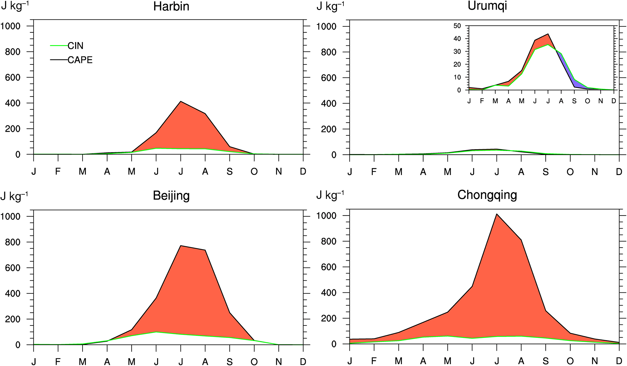
Figure 8 Annual cycle of CAPE (black line) and CIN (green line) values of four representative stations (Harbin, Urumqi, Beijing, and Chongqing). The orange filled area indicates values of CAPE with CIN deducted, i.e., real latent instability.

Annual mean values of CAPE (Fig. 7a) generally increase from south to north, following the spatial distribution of the near-surface specific humidity and temperature (Riemann-Campe et al., 2009, and their Fig. 2). The maxima occur in the southern coastal areas (larger than 300 J kg⁻¹), where the surface temperature is high and moisture is abundant. There is also large CAPE stored in the atmosphere over the southern region of the Qinghai–Tibet Plateau. As the summer monsoon of southern Asia is established, warm moist air originating from the Bay of Bengal is blown to the Tibetan plateau (Romatschke et at., 2010), and hence a large value of CAPE exists. The minimal CAPE values are observed in the north, especially in the northwest i.e., the arid and relatively cold regions, where the value of CAPE is less than 30 J kg⁻¹. In contrast to relatively large values of CAPE, values of CIN over China range from 4 to 70 J kg⁻¹ (Fig. 7b). Smaller values of CIN occur in the same region, where smaller CAPE values are observed. Large CIN values are observed in the Sichuan basin, indicating the need for stronger forcing to overcome a stable atmospheric layer for the occurrence of a wet convection. As a variable indicating real latent instability, annual mean CAPE_CIN (Fig. 7c) is spatially distributed similarly to CAPE. In general, smaller values are observed in the northwest of China (less than 10 J kg⁻¹) and larger values occur in the southernmost part of the country and south of the Qinghai–Tibet Plateau (larger than 300 J kg⁻¹).

Generally, the value of CAPE_CIN is largest in summer (Fig. S3). The annual cycles of CAPE and CIN of four representative stations (Harbin, Urumqi, Beijing, and Chongqing) are investigated (Fig. 8). CAPE values present a unimodal distribution. They generally increase in spring, achieve maxima in summer months, then begin to decrease during the autumn season, and reach minima in winter. The annual cycle of CIN of Harbin, Beijing, and Chongqing displays a similar distribution to that of CAPE, but is not as pronounced. As a result, CAPE of these three stations is much larger than the corresponding CIN during spring, summer, and autumn. Chongqing presents the largest value of CAPE and CAPE_CIN, indicating the largest probability of forming cumulus convection. In contrast, the CIN value of Urumqi is comparable to its CAPE. Both of them are very small, ranging from 0 to 50 J kg⁻¹. In addition, the value of CIN is less than or almost equal to CAPE in the autumn and winter months. Under such circumstances, destabilization will not occur, even if the layer has been lifted sufficiently.

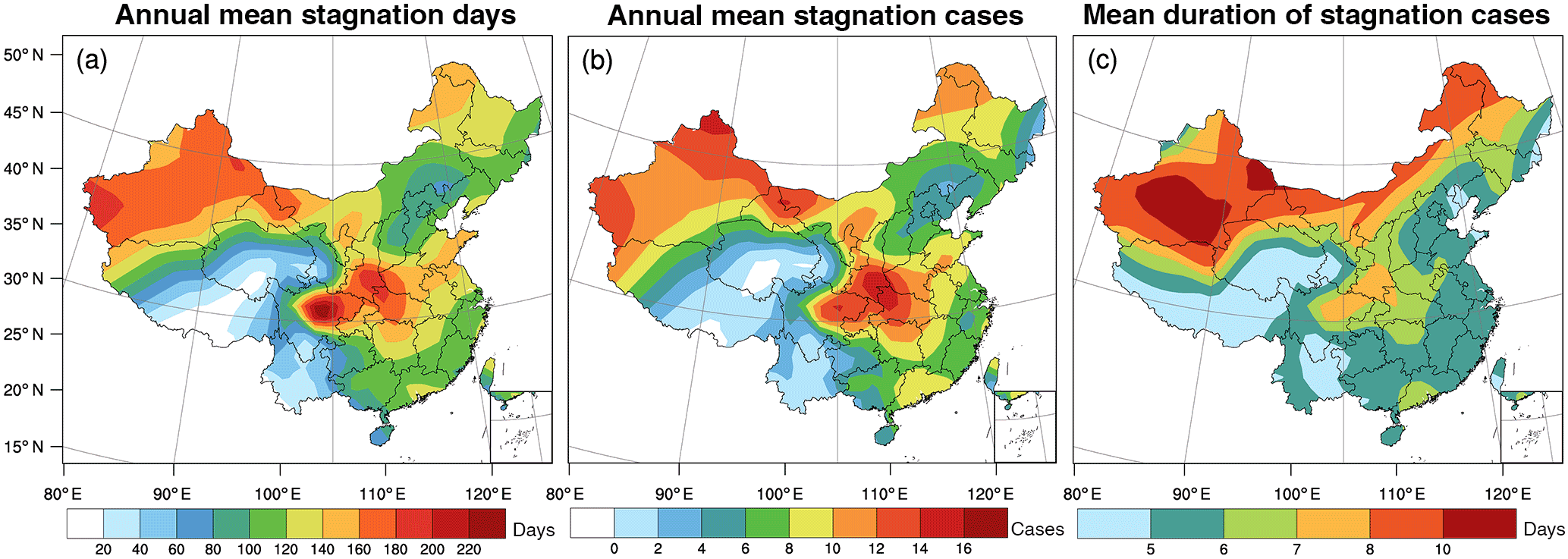
Figure 9 The spatial distribution of annual mean stagnation days (a), stagnation cases (b), and duration of stagnation cases (c) under new metrics.

4 Climatological results of the BSI

The national distribution of the annual mean of the BSI during 1985–2014 is displayed in Fig. 9. Results show that the spatial distributions of boundary-layer air stagnation days and cases are basically consistent with the old ones displayed in Huang et al. (2017). The new stagnation days and cases are still prevalent over the Xinjiang and Sichuan basins (more than 180 days and 14 cases per year) and barely occur over the Qinghai–Tibet and Yunnan plateaus (less than 40 days and two cases per year). However, the distribution pattern of the duration of one stagnation case is changed under new criteria. Air stagnation cases persist longer in the northern part of China (more than 8 days) and then the central part (about 7 days). The longest duration is observed in the northwestern region of China (more than 10 days), instead of the south of this country in the earlier study (Huang et al., 2017). The shortest duration occurs over the Qinghai–Tibet and Yunnan plateaus (less than 5 days).

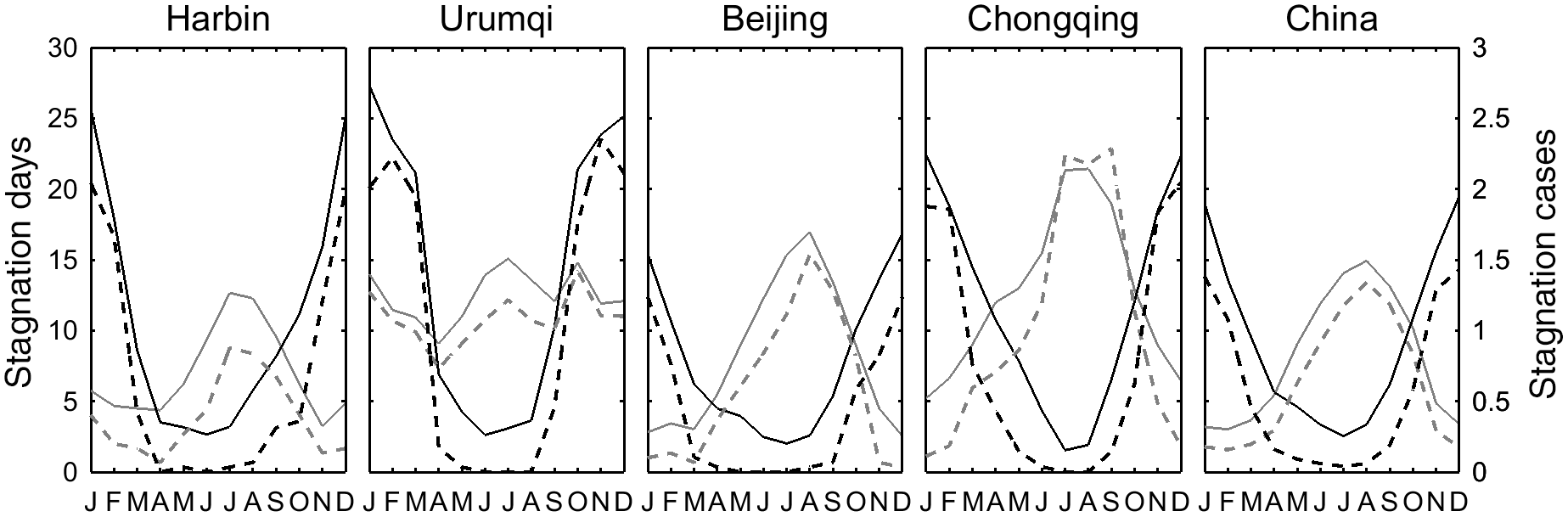
Figure 10 Annual cycles of air stagnation days and cases of four representative stations (Harbin, Urumqi, Beijing, and Chongqing), as well as the national average values. Black and grey lines indicate stagnation conditions under the BSI and ASI metrics, respectively. Solid and dash lines represent stagnation days and cases, respectively.

Much improved are the seasonal cycles of air stagnation days and cases. Generally, boundary-layer stagnant conditions occur most frequently in winter and least frequently in summer (Fig. S4). Results of monthly variations of four representative stations (Harbin, Urumqi, Beijing, and Chongqing), as well as the national averages, are displayed in Fig. 10. It is shown that stagnation days under the ASI metric are more in summer and less in winter. According to Huang et al. (2017), the behavior of upper-air wind speeds is the main driver of the ASI distribution. A weaker latitudinal pressure gradient at the upper layer of the atmosphere results in more air stagnation occurrences in summer. In contrast, the BSI is observed to be maximum in winter and minimum in summer. This behavior results from the cumulative responses of its components. We use standardized partial regression coefficients from multiple linear regression analysis to determine which variable is more important to BSI results (Table 1). It is shown that during the wintertime of Harbin, Urumqi, and Beijing, ventilation is the main driver of the BSI; precipitation contributes less; and cumulus convection barely plays a part in BSI results. In summer, however, ventilation and cumulus convection both contribute a lot. For Harbin, they play an almost equal role, with regression coefficients of 0.57 and 0.48, respectively. For Beijing, the contribution of CAPE outweighs that of ventilation by more than double. For Urumqi, which is in the semi-arid climate region, the ventilation is still the main driver of BSI behavior (β = 0.83), while precipitation and CAPE contribute equally (β = 0.36 and 0.4, respectively). The characteristics in Chongqing are different from the other three stations. With more convective energy stored in the atmosphere (Fig. 8), the seasonal variation of BSI relies more on CAPE: it is the second contributor during winter and spring (β = 0.36 and 0.38, respectively), and becomes the main contributor in summer and autumn (β = 0.75 and 0.68, respectively). Noticeably in summer, the BSI is dominated by cumulus convection, while the ventilation barely plays a role. The reason we add CAPE/CIN to the criteria is to make up for the deficiency of daily maximum mixing layer depth (MMD) derived from parcel method failing to describe the convection between the cloud base and cloud top. So it is expected that CAPE/CIN will play a more important role in summer.

Table 1 Dependence of BSI on its components, i.e., daily precipitation, ventilation and CAPE^*.

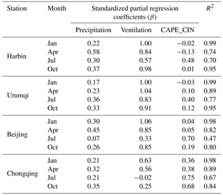
^* The relationships between monthly stagnation days and its corresponding components were derived by using multiple linear regression analysis. “Precipitation” stands for number of days with no precipitation; “Ventilation” for number of days when daily maximum ventilation is less than 6000 m² s⁻¹; “CAPE_CIN” for number of days when the value of CAPE is less than the absolute value of CIN.

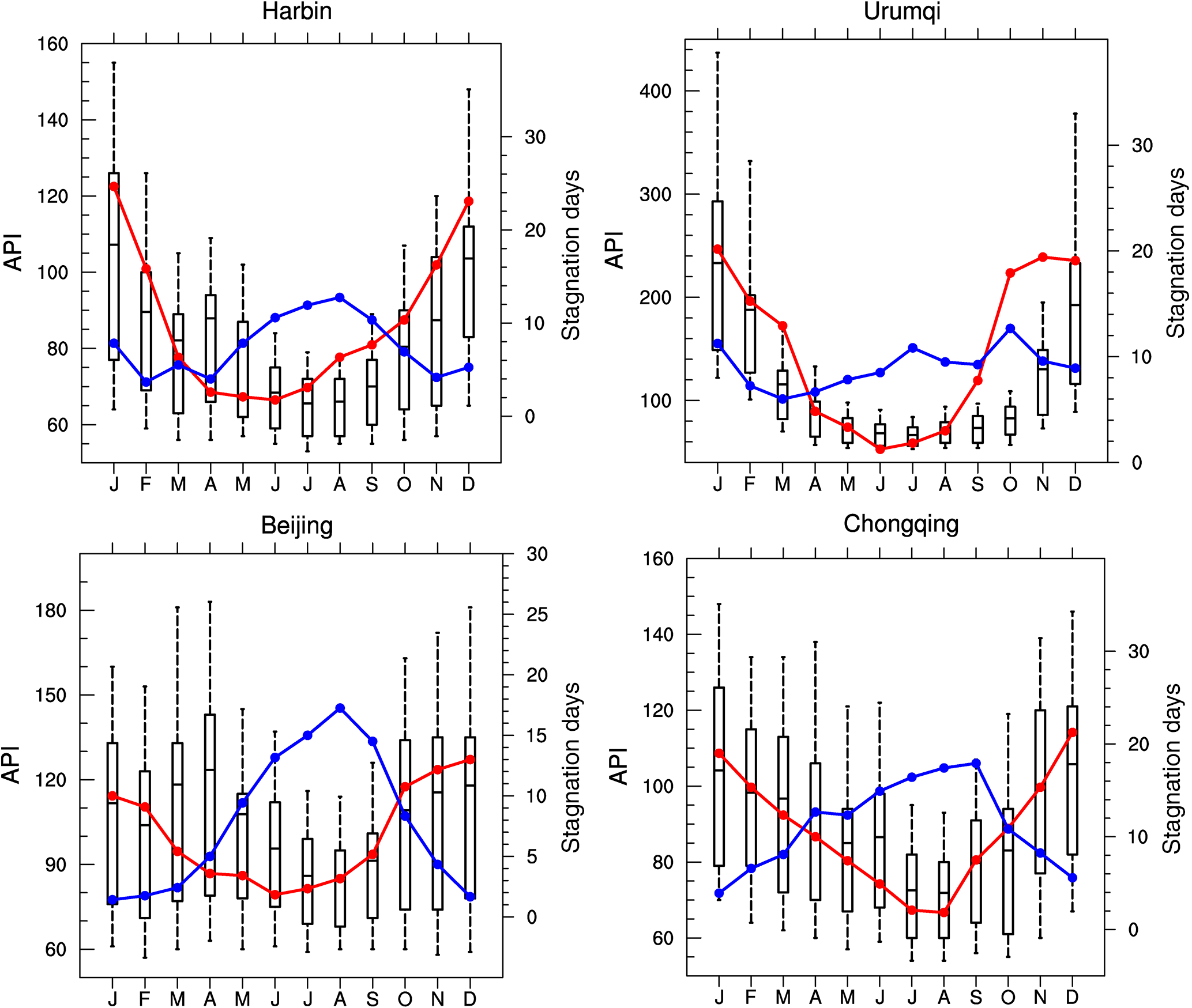
Figure 11 Monthly variations of the API averaged over 13 years (2000–2012), as well as the corresponding air stagnation days under the ASI and BSI criteria. Blue line: ASI; red line: BSI. Monthly mean values of the API are given as horizontal bars in the middle, 25 and 75 % percentiles are shown as boxes' lower and upper boundaries, and 10 and 90 % percentiles as lower and upper whiskers.

5 Correlations between the BSI and actual air pollution

The API as an indicator of air quality is used to testify the reasonability of the BSI. Figure 11 shows that monthly variations of the BSI can basically represent the annual cycles of the API. For all four representative stations, the annual cycle of boundary-layer air stagnation days reach maxima in winter and minima in summer, in agreement with the annual cycle of the API. However, there are two failures for the BSI to predict the API. One is the secondary peak of the API in spring for both Beijing and Harbin; the BSI cannot represent it. This is attributed to the influence of sand storms in spring in northern China. Sand storms usually result in a high level of particulate air pollution (high API), and are accompanied by strong winds and good ventilation conditions (low BSI). Another discrepancy is that the BSI during October to December of Urumqi is equally poor, whereas the corresponding API grows significantly during these 3 months. We cannot explain this discrepancy till now. The ASI is also shown in Fig. 11. Obviously, the BSI performs much better in indicating actual air pollution levels.

The correlations between monthly mean API and the total air stagnation days in this month are also investigated (Fig. 12). In order to exclude the impact of seasonal variation in source strengths, the investigation only covers data of the winter half-year (i.e., October–March) when domestic heating in northern China leads to more energy consumption and more serious air pollution pressure. With only data of the winter half-year analyzed, stagnation days under the BSI metric are generally larger than those under the ASI, since the occurrence of the BSI is more frequent in winter and less so in summer, while the ASI is the opposite (Fig. 10). Figure 12 shows that with the ASI criteria, monthly mean API has no evident correlation with monthly stagnation days, or even decreases with them (Chongqing), which is clearly irrational. Instead, with the BSI criteria, monthly mean API basically increases with the number of boundary-layer stagnation days, as we expected.

In addition, we have also explored the ability of the BSI to capture the air pollution days (Table 2). Every day during 2001–2012 is classified according to its API value. Then we calculated how many days in one category are considered air stagnation days under the ASI and BSI criteria. Results show that for moderate air quality with the API ranging from 50 to 100, the number of stagnation days that were identified by the BSI is almost the same as or even less than that by the ASI. For unhealthy air quality with the API ranging from 101 to 500, the percentage of identified air stagnation days with the BSI is basically more than that with the ASI; the former may even double or triple the latter in some situations. It suggests that the BSI has reduced the probability of misjudging an air pollution day and increased the chances of capturing the true one.

Table 2 How many days are identified as air stagnation days in each API category?

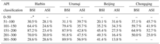
^* The result is ignored because there are fewer than 5 days falling into this category.

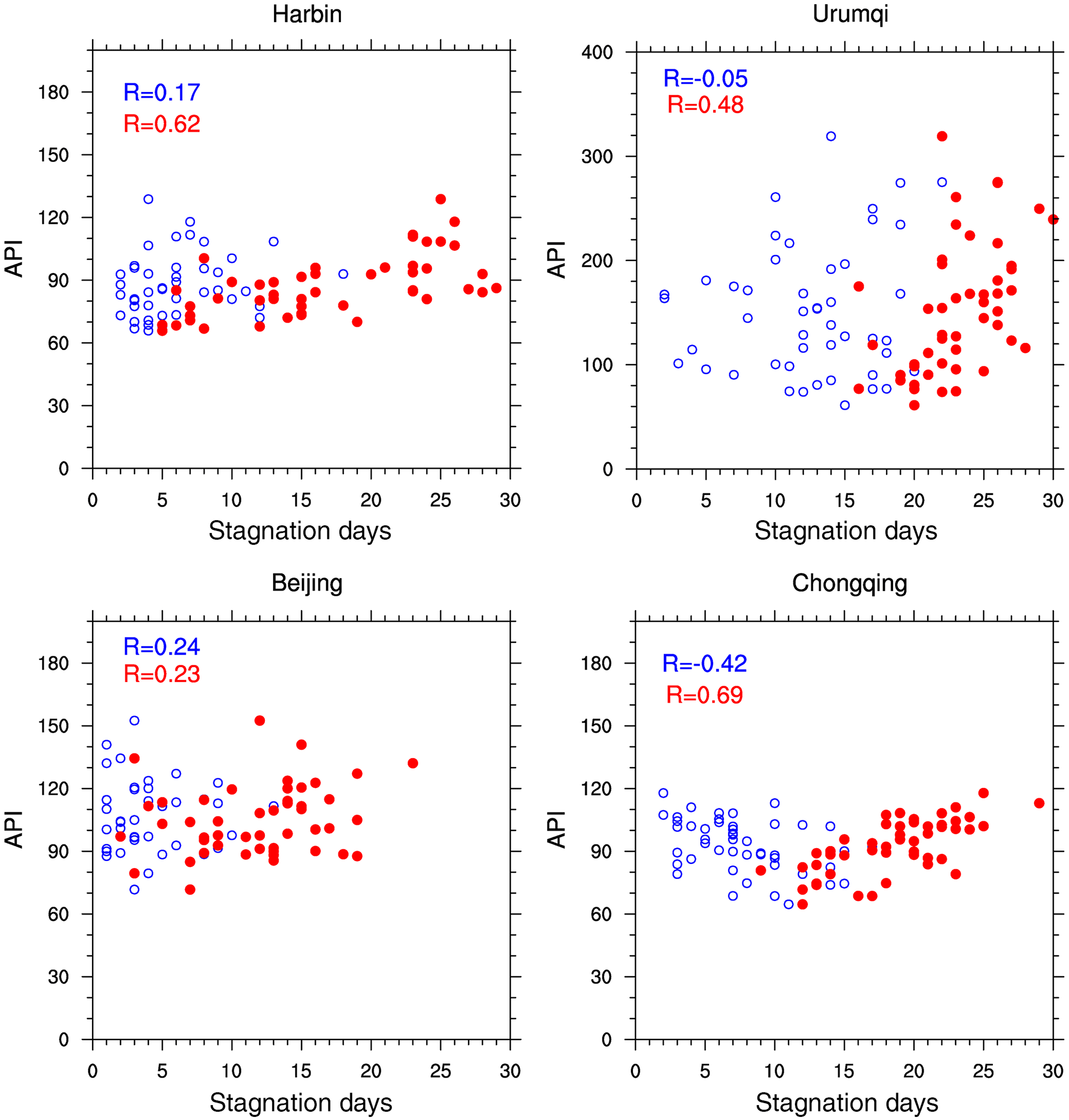
Figure 12 Correlations between monthly mean API and the total air stagnation days in the corresponding month in China winter half-year (October–March) during 2000–2012. R stands for correlation coefficient. Blue: ASI; red: BSI.

Apart from the statistical analysis of correlations between the API and BSI, we also conducted a case study about PM_2.5 concentrations and the BSI (Fig. 13). It is found that the BSI is able to track the day-by-day variation of an air pollution episode in January 2013 in Beijing which was characterized by continuous high PM_2.5 concentrations (Ji et al., 2014; Sun et al., 2014). The mean daily PM_2.5 concentration during that month ranged from 15.8 µg m⁻³ (1 January) to 568.6 µg m⁻³ (12 January). There were only 3 days when the PM_2.5 concentration reached the standard of less than 25 µg m⁻³ for the 24 h average suggested by the Air Quality Guidelines (AQG) of the World Health Organization (WHO; WHO, 2005), and only 7 days met the China National Ambient Air Quality Standards (CNAAQS; 75 µg m⁻³ for the 24 h average). In particular, the record-breaking hourly concentration of PM_2.5 reached as high as 886 µg m⁻³ at 19:00 LT (local time) on 12 January, exceeding more than 11 times the CNAAQS and 35 times the WHO AQG.

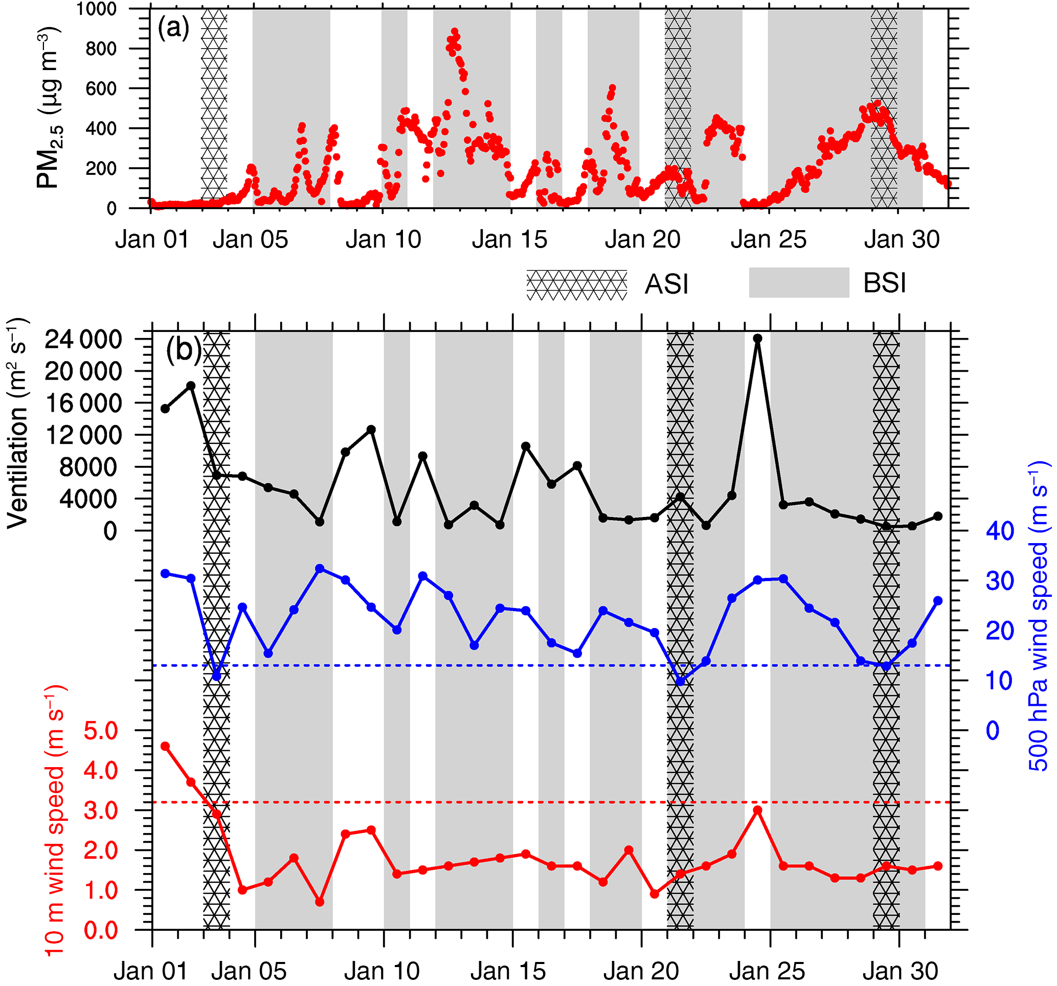
Figure 13 Time series of the ASI and BSI with hourly concentration of PM_2.5 during January 2013 of Beijing (a), and the corresponding variation of the main components of the ASI and BSI, i.e., daily ventilation and 500 hPa and 10 m wind speeds (b).

Ordinarily, emissions from one particular region remain constant over a short period. Therefore, the day-by-day variation of local air quality mainly depends on its weather conditions. Hourly concentration of PM_2.5 of Beijing and air stagnation days during January 2013 are presented in Fig. 13, as well as the components of both the ASI and BSI. According to weather records, no precipitation is reported in this month except on 20 and 31 January. In addition, the values of CAPE and CIN are nearly zero in the winter season, as mentioned above. Therefore, we only focus on the ventilation condition of the BSI, and 500 hPa and 10 m wind speeds of the ASI. It is seen that there are two long-duration haze episodes, i.e., 10–14 and 25–30 January, and some minor PM_2.5 concentration peaks on 6–7, 16, 18–19, and 21–23 January during this month. The ASI only successfully captures one heavy pollution on 29 January and one moderate pollution on 21 January. But it fails to capture other heavily polluted days, and misjudges a clean day (3 January) as a pollutant accumulation day. The reason is that although 10 m wind speed falls below the 3.2 m s⁻¹ standard since 3 January, 500 hPa wind speed – the dominant component in the ASI (Huang et al., 2017) – is generally above the 13 m s⁻¹ standard except for 3, 21, and 29 January. It verifies again that 500 hPa wind speed is not appropriate to be an ASI element. The boundary-layer air stagnation pattern matches the day-by-day variation of PM_2.5 concentration pretty well. The two major and four minor haze episodes are all successfully identified as boundary-layer air stagnation days, except 11 January. It should be reasonable since even though the daily mean concentration of PM_2.5 on 11 January was relatively high, its hourly concentration actually decreased throughout the day. Correspondingly, this day presents a good ventilation condition (9328 m² s⁻¹; Fig. 13b) and is identified as a non-stagnation day.

We also investigated the time series of daily PM_2.5 concentration in Beijing during November and December in 2015–2017, as well as the stagnation days under the ASI and BSI metrics (Fig. 14), to further demonstrate the performance of the BSI. It is shown that the BSI is a better metric for capturing the meteorological conditions conducive to poor air quality. Nearly all the peaks of PM_2.5 concentration or its accumulating processes correspond to boundary-layer stagnant days. Compared to 2015 and 2016, PM_2.5 concentration during November and December in 2017 was significantly reduced. The 24-averaged PM_2.5 concentration was less than 50 µg m⁻³ on 70 % of the days and larger than 150 µg m⁻³ on only 3 days. Correspondingly, boundary-layer stagnant days were greatly reduced, especially stagnant cases. Fewer stagnant cases mean smaller meteorological potential for air pollutants to accumulate. As a result, air quality during the late autumn and early winter in 2017 was largely improved. Figure 15 shows that the averaged concentration of PM_2.5 during these 2 months in 2015–2017 negatively correlates with the number of boundary-layer stagnation days. It illustrates that an increase in the capacity of the atmospheric environment plays an important role in air quality improvement during November and December in 2017, and the BSI successfully represents this trend.

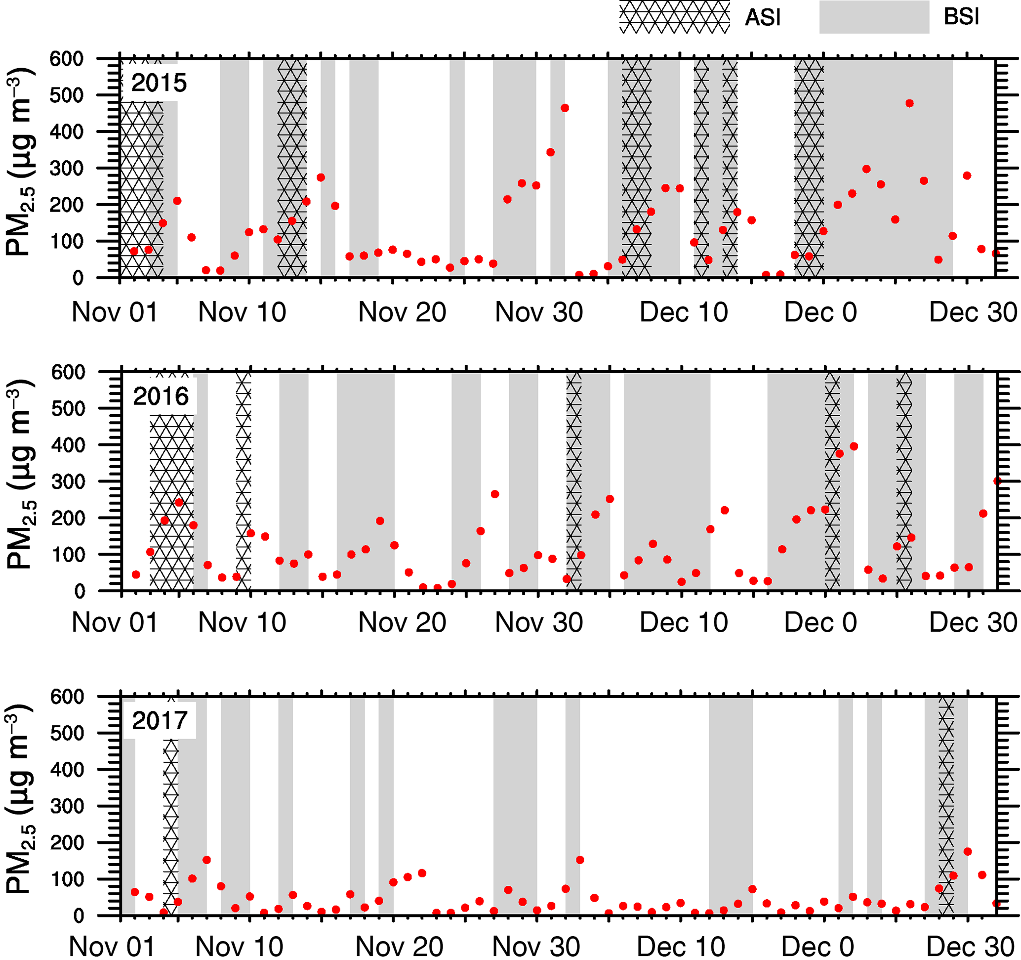
Figure 14 Time series of 24 h averaged concentration of PM_2.5 of Beijing from November to December during 2015–2017. Stagnation days under the ASI and BSI metrics are marked with stripes and grey colors, respectively.

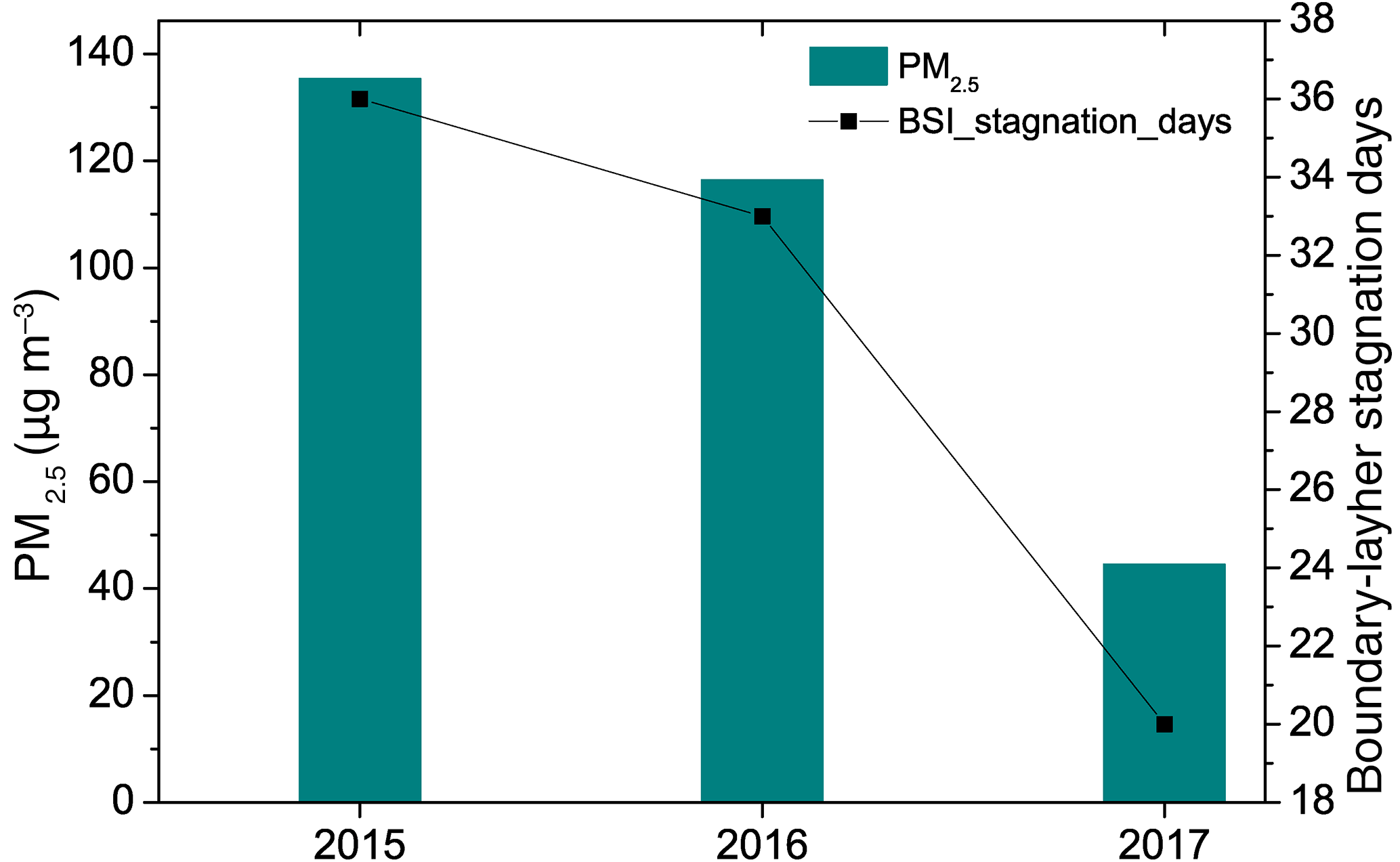
Figure 15 Averaged concentration of PM_2.5 during November and December in 2015–2017, and the corresponding number of boundary-layer stagnation days.

However, we do not expect that the BSI will perform well in capturing air pollution episodes in spring and summer. The reason is that this metric only indicates adverse meteorological conditions to air pollution, without the influences of emissions or chemical reactions in the atmosphere. In spring, air quality of Beijing is greatly deteriorated by frequent sand storms (He et al., 2001), which are often accompanied by strong winds and good ventilation conditions (low BSI). This results in great discrepancies between the BSI and actual air quality (Fig. 11). During summer, highly oxidative atmosphere and secondary formation of aerosols are the main problems (Fu et al., 2014; Ran et al., 2011). As a result, the BSI may not be able to track the actual air pollution episodes during these two seasons.

6 Conclusion

Meteorological background is critical to the occurrence of air pollution events, since it determines the accumulation or dilution of air pollutants. The United States adopts the Air Stagnation Index (ASI) to measure the meteorological state, taking 500 hPa and 10 m wind speeds, and precipitation into consideration. However, this metric is found to be not very adequate for China. Taking Beijing as an example, strong upper-level wind occurs on 75 % of most polluted days (the API ranks in the 90th percentile or higher). It means that strong upper-air winds do not necessarily drive the near-surface dispersion of air pollutants. In the present study, we proposed a new metric for the ASI–Boundary-layer air Stagnation Index (BSI), based on (i) daily maximal ventilation, indicating horizontal dilution and vertical mixing extent in the boundary layer, (ii) real latent instability, implying the convection between the layer of cloud base and cloud top, and (iii) precipitation, representing the washout effects of air pollutants.

Based on sounding data and hourly near-surface temperature observations, we firstly calculated daily maximum mixing layer depth during 1985–2014, and then estimated daily maximal ventilation in the boundary layer. Combined with daily precipitation and CAPE and CIN values, we derived results of the BSI of 66 stations across the country, and investigated the climatological features of them. It shows that the BSI maintains a similar spatial pattern in comparison with the ASI (Huang et al., 2017). Annual mean stagnation days under the BSI metric are most prevalent (more than 180 days) over the northwestern and southwestern basins, i.e., Xinjiang and Sichuan basins, and least (less than 40 days) over the Qinghai–Tibet and Yunnan plateaus. However, the annual cycle of the boundary-layer stagnation days is different, with the frequency of stagnation occurrences reaching a maximum in winter and minimum in summer, which is contrary to the ASI result. The seasonal variation of the BSI is the cumulative response of its components (ventilation, precipitation, and cumulus convection). It is dominated by the ventilation coefficient during winter and influenced by the combined results of all components in summer.

The annual cycle of boundary-layer stagnation days is consistent with the monthly variation of API during 2000–2012. Moreover, the BSI shows a positive correlation with API during the boreal winter half-year, and is found to be more efficient in identifying unhealthy air quality, with the API ranging from 101 to 500. In addition, the BSI also tracks the day-by-day variation of PM_2.5 concentration well during the record-breaking haze episodes in January 2013 in Beijing and successfully represents the improved air quality during November and December in 2017. Therefore, the BSI may act as a better indicator of atmospheric dispersion and dilution in air pollution research.

Appendix A

Table A1 The information of 66 stations used in this study. Date ranges are the periods when radiosonde data, daily precipitation, and daily maximum temperature are all available at the same time. The periods less than 30 years are highlighted in bold. The percentages of valid data are presented. Data periods of less than 30 years are highlighted in bold.

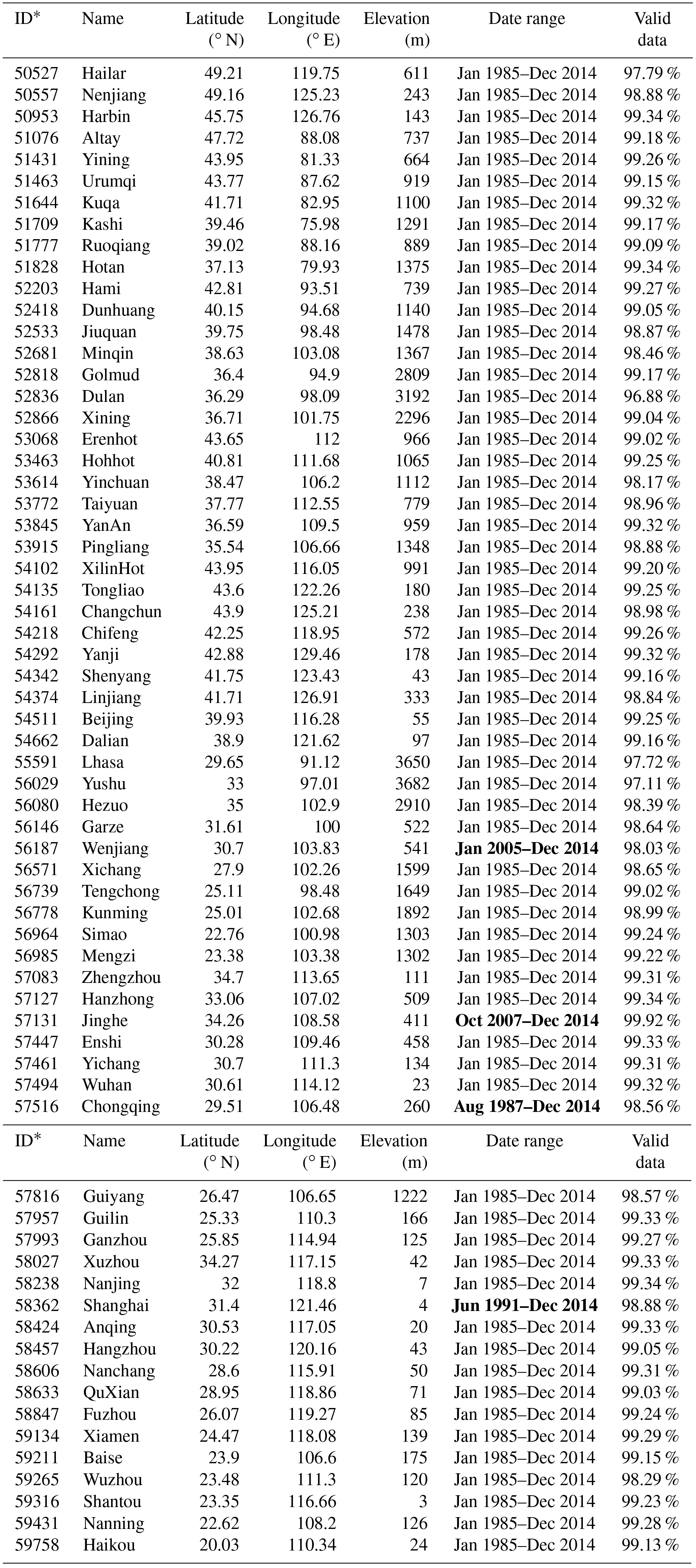
^* World Meteorological Organization Identification Number.