Simulation of fine organic aerosols in the western Mediterranean area during the ChArMEx 2013 summer campaign

The simulation of fine organic aerosols with CTMs (chemistry–transport models) in the western Mediterranean basin has not been studied until recently. The ChArMEx (the Chemistry-Aerosol Mediterranean Experiment) SOP 1b (Special Observation Period 1b) intensive field campaign in summer of 2013 gathered a large and comprehensive data set of observations, allowing the study of different aspects of the Mediterranean atmosphere including the formation of organic aerosols (OAs) in 3-D models. In this study, we used the CHIMERE CTM to perform simulations for the duration of the SAFMED (Secondary Aerosol Formation in the MEDiterranean) period (July to August 2013) of this campaign. In particular, we evaluated four schemes for the simulation of OA, including the CHIMERE standard scheme, the VBS (volatility basis set) standard scheme with two parameterizations including aging of biogenic secondary OA, and a modified version of the VBS scheme which includes fragmentation and formation of nonvolatile OA. The results from these four schemes are compared to observations at two stations in the western Mediterranean basin, located on Ersa, Cap Corse (Corsica, France), and at Cap Es Pinar (Mallorca, Spain). These observations include OA mass concentration, PMF (positive matrix factorization) results of different OA fractions, and ¹⁴C observations showing the fossil or nonfossil origins of carbonaceous particles. Because of the complex orography of the Ersa site, an original method for calculating an orographic representativeness error (ORE) has been developed. It is concluded that the modified VBS scheme is close to observations in all three aspects mentioned above; the standard VBS scheme without BSOA (biogenic secondary organic aerosol) aging also has a satisfactory performance in simulating the mass concentration of OA, but not for the source origin analysis comparisons. In addition, the OA sources over the western Mediterranean basin are explored. OA shows a major biogenic origin, especially at several hundred meters height from the surface; however over the Gulf of Genoa near the surface, the anthropogenic origin is of similar importance. A general assessment of other species was performed to evaluate the robustness of the simulations for this particular domain before evaluating OA simulation schemes. It is also shown that the Cap Corse site presents important orographic complexity, which makes comparison between model simulations and observations difficult. A method was designed to estimate an orographic representativeness error for species measured at Ersa and yields an uncertainty of between 50 and 85 % for primary pollutants, and around 2–10 % for secondary species.

1 Introduction

The Mediterranean basin is subject to multiple emission sources; anthropogenic emissions that are transported from adjacent continents or are produced within the basin, local or continental biogenic and natural emissions among which the dust emissions from northern Africa can be considered as an important source (Pey et al., 2013; Vincent et al., 2016). All these different sources, the geographic particularities of the region favoring accumulation of pollutants (Gangoiti et al., 2001), and the prevailing meteorological conditions favorable to intense photochemistry and thus secondary aerosol formation, make the Mediterranean area a region experiencing a heavy burden of aerosols (Monks et al., 2009; Nabat et al., 2012). In the densely populated coastal areas, this aerosol burden constitutes a serious sanitary problem considering the harmful effects of fine aerosols on human health (Martinelli et al., 2013). In addition, studies have shown that the Mediterranean area could be highly sensitive to future climate change effects (Giorgi, 2006; Lionello and Giorgi, 2007). This could affect aerosol formation processes, but in turn the aerosol load also affects regional climate (Nabat et al., 2013). These interactions, the high aerosol burden in the area, and its health impact related to the high population density situated around the basin make this region particularly important to study.

The aforementioned primary emissions can be in the form of gaseous species, as particulate matter, or as semi-volatile species distributed between both phases (Robinson et al., 2007). In the atmosphere, they can subsequently undergo complex chemical processes lowering their volatility, which leads to the formation of secondary particles. These processes are not entirely elucidated especially for the formation of SOAs (secondary organic aerosols) for example (Kroll and Seinfeld, 2008), starting from initially emitted biogenic or anthropogenic VOCs (volatile organic compounds) and SVOCs (semi-volatile organic compounds).

The chemical composition of aerosols has been studied in detail in the eastern Mediterranean area (Lelieveld et al., 2002; Bardouki et al., 2003; Sciare et al., 2005, 2008; Koçak et al., 2007; Koulouri et al., 2008) and to a lesser extent in the western part (Sellegri et al., 2001; Querol et al., 2009; Minguillón et al., 2011; Ripoll et al., 2014; Menut et al., 2015; Arndt et al., 2017). Little focus has been given to the formation of organic aerosol (OA) over the western Mediterranean even if OA can play a significant role in both local and global climate (Kanakidou et al., 2005) and can affect health (Pöschl, 2005; Mauderly and Chow, 2008). Its contribution has been calculated in studies to be nearly 30 % in PM₁ for the eastern Mediterranean area during the FAME 2008 campaign (i.e., Hildebrandt et al., 2010). It is also important to know the contribution of different sources (biogenic, anthropogenic) to the total concentration of OA in the western part of the basin. Such studies have been performed for the eastern Mediterranean basin (e.g., Hildebrandt et al., 2010), while for the western part of the basin, they have been in general restricted to coastal cities such as Marseilles and Barcelona (El Haddad et al., 2011; Mohr et al., 2012; Ripoll et al., 2014).

The ChArMEx (the Chemistry Aerosol Mediterranean Experiment; http://charmex.lsce.ipsl.fr, last access: 17 August 2016) project was organized in this context, with a focus over the western Mediterranean basin during the period of 2012–2014, in order to better assess the sources, formation, transformation, and mechanisms of transportation of gases and aerosols. During this project, detailed measurements were acquired not only for the chemical composition of aerosols but also for a large number of gaseous species from both ground-based and airborne platforms. The project ChArMEx is divided into different sub-projects, each with a different goal; among those, the SAFMED (Secondary Aerosol Formation in the MEDiterranean) project aimed at understanding and characterizing the concentrations and properties of OA in the western Mediterranean (for example Nicolas, 2013; Di Biagio et al., 2015; Chrit et al., 2017; Arndt et al., 2017; Freney et al., 2017). To reach these goals, two intense ground-based and airborne campaigns were organized during July–August of 2013 and also summer of 2014. The focus of the present study is on the SAFMED campaign in summer of 2013, since detailed measurements on the formation of OA and precursors were obtained during this period, namely at Ersa (Corsica) and Es Pinar (Mallorca). Other ChArMEx sub-projects and campaigns included the TRAQA (Transport et Qualité de l'Air) campaign in summer 2012, set up to study the transport and impact of continental air on atmospheric pollution over the basin (Sič et al., 2016), and the ADRIMED (Aerosol Direct Radiative Impact on the regional climate in the MEDiterranean, June–July 2013) campaign aimed at understanding and assessing the radiative impact of various aerosol sources (Mallet et al., 2016).

Modeling of aerosol processes and properties is a difficult task. Aside from the lack of knowledge of aerosol formation processes, the difficulty lies in the fact that OAs present an amalgam of thousands of different species that cannot all be represented in a 3-D chemistry–transport model (CTM) due to limits in computational resources. Therefore a small number of lumped species with characteristics that are thought to be representative of all the species in each group are used instead. There are many different approaches that can be used in creating representative groups for OAs (e.g., which characteristics to use to group the species, which species to lump together, physical processes that should be presented for their simulation). It is therefore necessary to test these different simulation schemes for OAs in different regions and compare the results to experimental data to check for their robustness. For example, Chrit et al. (2017) modeled SOA formation in the western Mediterranean area during the ChArMEx summer campaigns, with a surrogate scheme that also contains ELVOCs (extremely low-volatility organic compounds). The simulated concentrations and properties (oxidation and affinity with water) of OAs agree well with the observations performed at Ersa (Corsica), after they had included the formation of extremely low-volatility OAs and organic nitrate from monoterpene oxidation in the model.

The present study focuses on the comparison of different OA formation schemes implemented in the CHIMERE chemistry–transport model for simulation of OA over the western Mediterranean area. Different configurations of the volatility basis set (VBS; Donahue et al., 2006; Robinson et al., 2007; Shrivastava et al., 2013) and the base parameterization of the CHIMERE 3-D model (Bessagnet et al., 2008; Menut et al., 2013) are used for this purpose. Our work takes advantage of the extensive experimental data pool obtained during the SAFMED campaign. This enables us to perform model–observation comparisons with unprecedented detail over this region, including not only the OA concentration but also its origin (¹⁴C analyses) and its oxidation state (positive matrix factorization (PMF) method results). In addition, a comparison for meteorological parameters and gaseous or particulate species which could affect the production of OA or could help analyze the robustness of the used schemes has been performed. Moreover, because of the orographic complexity of one of the sites (Ersa, Cap Corse) explored in this work, a novel method is designed to calculate the orographic representativeness error of different species. To the best of our knowledge, this is the first time that the concentrations of precursors, intermediary products, and OA concentrations and properties have been simulated for different OA simulation schemes and compared for each scheme to multiple series of measurements at different stations for the western Mediterranean area. For OA schemes, the paper aims at assessing the robustness of each scheme with regard to different criteria as mass, fossil, and modern fraction and volatility. Section 2 describes the model and the inputs used for the simulations. Also, the evaluated schemes are explained in this section in more detail. The experimental data used for simulation–observation comparisons are discussed in Sect. 3. An overall validation of the model is presented in Sect. 4, together with comparisons of different gaseous and particulate species and meteorological parameters to observations. In Sect. 5, comparison of implemented schemes to measurements regarding concentration, oxidation state, and origin of OA is presented. In Sect. 6, the contribution of different sources to the OA present in the whole basin is explored, before the conclusion in Sect. 7.

2 Model setup

The CHIMERE model (Menut et al., 2013; http://www.lmd.polytechnique.fr/chimere, last access: 9 August 2016) is an offline regional CTM which has been tested rigorously for Europe and France (Zhang et al., 2013; Petetin et al., 2014; Colette et al., 2015; Menut et al., 2015; Rea et al., 2015). It is also widely used in both research and forecasting activities in France, Europe, and other countries (Hodzic and Jimenez, 2011). In this work, a slightly modified version of the CHIMERE 2014b configuration is used to perform the simulations. The modifications concern an updated description of the changes in aerosol size distribution due to condensation and evaporation processes (Mailler et al., 2017). Four domains are used in the simulations: a coarse domain covering all of Europe and northern Africa with a 30 km resolution, and three nested domains inside the coarse domain with resolutions of 10, 3, and 1 km (Fig. 1). The 10 km resolved domain covers the western Mediterranean area and the two smaller domains are centered on the Cap Corse, where the main field observations in SAFMED were performed. Such highly resolved domains are necessary to resolve the complex orography of the Cap Corse ground-based measurement site, which will be discussed in Sect. 4, while for the flatter Es Pinar site, a 10 km resolution is sufficient. The simulations for each domain contain 15 vertical levels starting from 50 m to about 12 km above sea level (a.s.l.) with an average vertical resolution of 400 m within the continental boundary layer and 1 km above. The CHIMERE model needs a set of gridded data as mandatory input: meteorological data, emission data for both biogenic and anthropogenic sources, land use parameters, boundary and limit conditions, and other optional inputs such as dust and fire emissions. Given these inputs, the model produces the concentrations and deposition fluxes for major gaseous and particulate species and also intermediate compounds. The simulations presented in this article cover the period of 1 month from 10 July to 9 August.

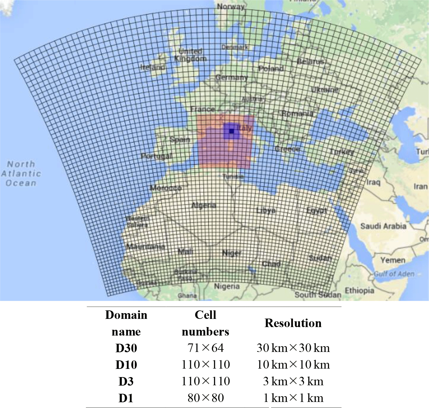
Figure 1 The four domains used in simulations (D30, D10, D3, D1). The resolution for each domain is given in the table below the image.

Meteorological inputs are calculated with the WRF (Weather Research Forecast) regional model (Wang et al., 2015) forced by NCEP (National Centers of Environmental Predictions) reanalysis meteorological data (http://www.ncep.noaa.gov, last access: 11 September 2016) with a base resolution of 1^∘. Slightly larger versions of each domain with the same horizontal resolutions (Fig. 1) are used for the meteorological simulations. The WRF configuration used for this study consists of the single-moment 5 class microphysics scheme (Hong et al., 2004), the Rapid Radiative Transfer model (RRTMG) radiation scheme (Mlawer et al., 1997), the Monin–Obukhov surface layer scheme (Janjic, 2003), and the NOAA Land Surface Model scheme for land surface physics (Chen et al., 2001). Sea surface temperature update, surface grid nudging (Liu et al., 2012; Bowden et al., 2012), ocean physics, and topographic wind options are activated. Also, the feedback option is activated, meaning that the simulation of the nested domains can influence the parent domain. Some observation–simulation comparisons are presented for meteorological parameters in Sect. 4.

Anthropogenic emissions for all but shipping SNAP (Selected Nomenclature for Air Pollution) sectors come from the HTAP-V2 (Hemispheric Transport of Air Pollution; http://edgar.jrc.ec.europa.eu/htap_v2/index.php, last access: 21 August 2016) inventory. The shipping sector in this inventory was judged to overestimate ship traffic around the Cap Corse area, especially on the shipping lines between Marseilles and Corsica, due to overweighing ferries with respect to cargos (Van der Gon, personal communication). This could be explained by the fact that the boat traffic description is based on voluntary information. Therefore HTAP-V2 shipping emissions were replaced by those of the MACC-III inventory (Kuenen et al., 2014). The base resolution of the HTAP inventory is 10 km × 10 km and that of the MACC-III inventory is 7 km × 7 km. For both inventories the emissions for the year 2010 were used since this year was the latest common year in the two inventories.

Biogenic emissions are calculated using MEGAN (Model of Emissions of Gases and Aerosols from Nature; Guenther et al., 2006) including isoprene, limonene, α-pinene, β-pinene, ocimene, and other monoterpenes with a base horizontal resolution of 0.008^∘ × 0.008^∘. The land use data come from GlobCover (Arino et al., 2008) with a base resolution of 300 m × 300 m. Initial and boundary conditions of chemical species are taken from the climatological simulations of LMDz-INCA3 (Hauglustaine et al., 2014) for gaseous species and GOCART (Chin et al., 2002) for particulate matter.

The chemical mechanism used for the baseline gas-phase chemistry is the MELCHIOR2 scheme (Derognat et al., 2003). This mechanism has around 120 reactions to describe the whole gas-phase chemistry. The reaction rates used in MELCHIOR are constantly updated (last update in 2015); however, the reaction scheme itself has not been updated since 2003. Some reactions have been added to it by Bessagnet et al. (2009) regarding the oxidation of OA precursors, but they do not affect gas-phase chemistry. Also, MELCHIOR has been compared to SAPRC-07A, a more recent scheme (Carter, 2010), and the results show acceptable differences between the two schemes; for example, when compared to EEA (European Economic Area) ozone measurements, both produce a correlation coefficient of 0.71. These comparisons are presented in Menut et al. (2013) and Mailler et al. (2017).

The CHIMERE aerosol module is responsible for the simulation of physical and chemical processes that influence the size distribution and chemical speciation of aerosols (Bessagnet et al., 2008). This module distributes aerosols in a number of size bins; here 10 bins range from 40 nm to 40 µm, in a logarithmic sectional distribution, each bin spanning over a size range of a factor of 2 (40–20, 20–10 µm, etc.). The module also addresses coagulation, nucleation, condensation, and dry and wet deposition processes. The basic chemical speciation includes elemental carbon (EC), sulfate, nitrate, ammonium, SOA, dust, salt, and PPM (primary particulate matter other than ones mentioned above).

2.1 Organic aerosol simulation

The SOA particles are divided, depending on their precursors, into two groups: ASOA (anthropogenic SOA) and BSOA (biogenic SOA). Four schemes were tested to simulate their formation; more detail on each scheme is presented below.

2.1.1 CHIMERE standard scheme

The SOA simulation scheme in CHIMERE (Bessagnet et al., 2008) consists of a single-step oxidation process in which VOC lumped species are directly transformed into SVOCs with yields that are taken from experimental data (Odum et al., 1997; Griffin et al., 1999; Pun and Seigneur, 2007). These SVOC species are then distributed into gaseous and particulate phases (Fig. 2a) following the partitioning theory of Pankow (Pankow, 1987). The precursors for this scheme are presented in the Supplement (Sect. SI1). A number of 11 semi-volatile surrogate compounds are formed from these precursors, which include six hydrophilic species, three hydrophobic species, and two surrogates for isoprene oxidation. The sum of all 11 species results in the concentration of simulated SOA in this scheme.

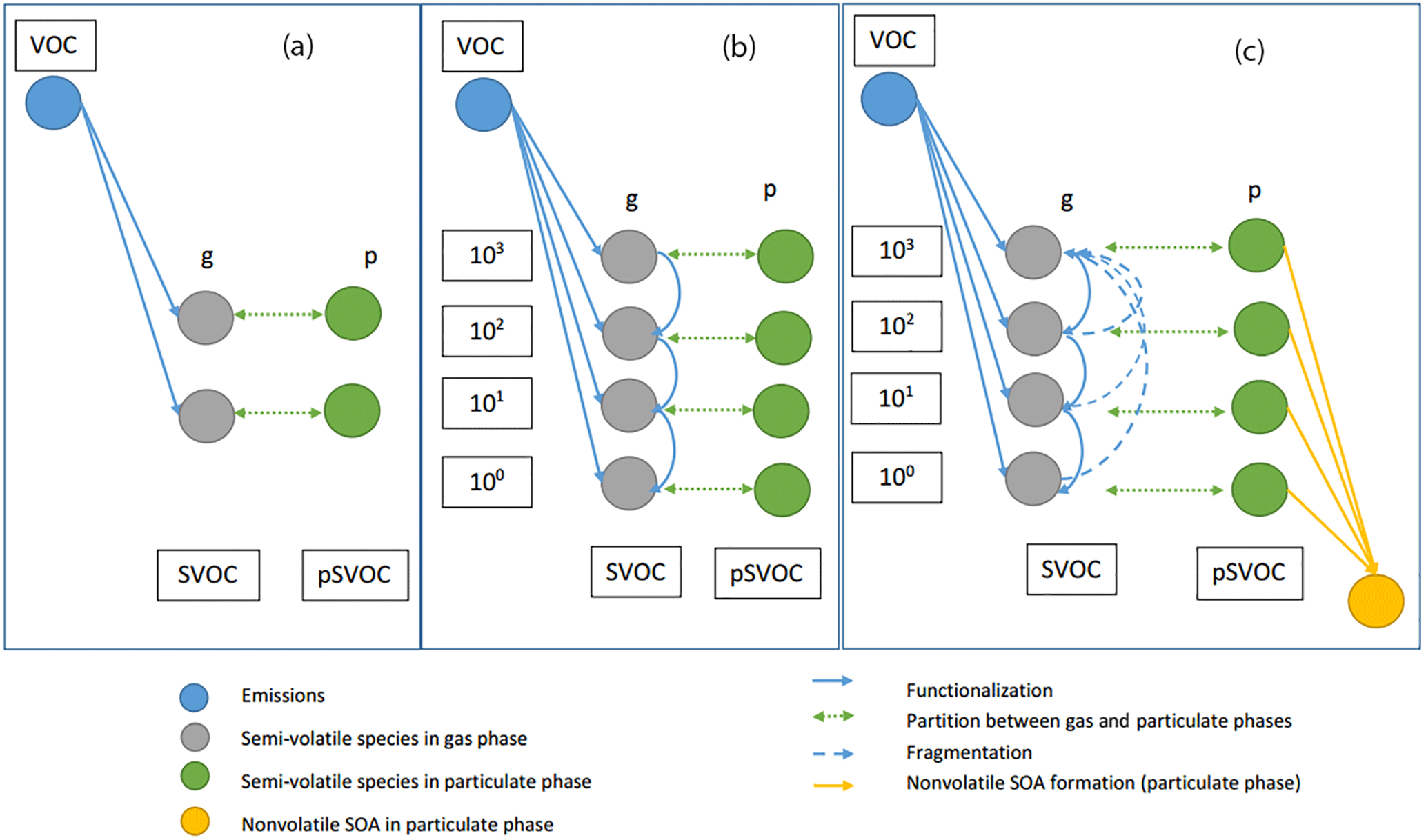
Figure 2 Organic aerosol simulation schemes. (a) CHIMERE standard scheme (Bessagnet et al., 2008): from a parent volatile organic compound (VOC), different semi-volatile organic compounds (SVOCs) (only one represented) are formed in a single step by oxidation; they are in equilibrium between gas and aerosol phases (pSVOC); (b) VBS standard scheme (Robinson et al., 2007): from a parent VOC, SVOCs with regularly spaced volatility ranges are formed and are in equilibrium with the aerosol phase. Aging of SVOC by functionalization is included by passing species to classes with lower volatility; (c) modified VBS scheme (Shrivastava et al., 2015): here SVOC aging also includes fragmentation, leading to transfer of species to classes with higher volatility. In addition, semi-volatile aerosol can be irreversibly transformed into nonvolatile aerosol (yellow-filled circle). For each bin, saturation concentration is shown in micrograms per cubic meter. Note that this schematic represents BSOA and ASOA (biogenic and anthropogenic secondary organic aerosol) where four bins are used; for SVOC and IVOC (semi-volatile and intermediate-volatility organic compounds, where nine bins are used) a schematic is presented in Supplement Sect. SI1.

2.1.2 VBS scheme

As an alternative to single-step schemes like the one in CHIMERE, the VBS approach was developed. In these types of schemes, SVOCs are divided into volatility bins regardless of their chemical characteristics, but only depending on their saturation concentration. Therefore it becomes possible to add aging processes in the simulation of OA by adding reactions that shift species from one volatility bin to another (Donahue et al., 2006). This scheme was implemented and tested in CHIMERE for Mexico City (Hodzic and Jimenez, 2011) and the Paris region (Zhang et al., 2013). The volatility profile used for this scheme consists of nine volatility bins with saturation concentrations in the range of 0.01 to 10⁶ µg m⁻³ (convertible to saturation pressure using atmospheric standard conditions), across which the emissions of SVOCs and IVOCs are distributed, following a specific aggregation table (Robinson et al., 2007). Four volatility bins are used for ASOA and BSOA ranging from 1 to 1000 µg m⁻³. SOA yields are taken from the literature (Lane et al., 2008; Murphy and Pandis, 2009) using low-NO_x conditions (VOC ∕ NO_x>10 ppbC ppb⁻¹). The SVOC species can age, by decreasing their volatility by one bin independent of their origin with a given constant rate. SVOC species are either directly emitted or formed from anthropogenic or biogenic VOC precursors. Fragmentation processes and the production of nonvolatile SOAs are ignored in this scheme. In the basic VBS scheme, the BSOA aging processes are usually ignored since they tend to result in a significant overestimation of BSOA (Lane et al., 2008). Although physically present, their kinetic constants for this aging process are considered the same as anthropogenic compounds and seem to be overestimated. However, in Zhang et al. (2013), including BSOA aging was necessary to explain the observed experimental data. Therefore, in this work, the VBS scheme is evaluated both with and without including the BSOA aging processes. Figure 2b shows a simplified illustration for ASOA and BSOA, while the partition for SVOC is presented in the Supplement (Sect. SI2). For all bins, regardless of their origin, the partitioning between gaseous and the particulate phases is performed following Raoult's law and depends on total OA concentration. Under normal atmospheric conditions, SVOC with the volatility range of 0.01 to 10³ µg m⁻³ can form aerosols. In total, the sum of 24 species in the model (with 10 size distribution bins each, i.e., 240 species in total) makes up the total concentration of SOA simulated by this scheme.

2.1.3 Modified VBS scheme

The basic VBS scheme does not include fragmentation processes, corresponding to the breakup of oxidized OA compounds in the atmosphere into smaller and thus more volatile molecules (Shrivastava et al., 2011). It also does not include the formation of nonvolatile SOA, where SOA can become nonvolatile after formation (Shrivastava et al., 2015). In this work, these two processes were added to the VBS scheme presented above and tested for the Mediterranean basin. The volatility bins for the VBS model were not changed (ranges presented in the previous section). SOA yields were kept as in the standard VBS scheme; however, instead of using the low-NO_x or the high-NO_x regimes, an interpolation between the yields of these two regimes was added to the model. For this purpose, a parameter is added to the scheme, which calculates the ratio of the reaction rate of RO₂ radicals with NO (high-NO_x regime) with respect to the sum of reaction rates of the reactions with HO₂ and RO₂ (low-NO_x regime). For this purpose, a parameter (α) is added to the scheme, which calculates the ratio of the reaction rate of RO₂ radicals with NO (ν_NO; high-NO_x regime) with respect to the sum of reaction rates of the reactions with HO₂ (${\mathit{\nu }}_{{\mathrm{HO}}_{\mathrm{2}}})$ and RO₂ (${\mathit{\nu }}_{{\mathrm{RO}}_{\mathrm{2}}}$; low-NO_x regime). The parameter α is expressed as follows:

$$\begin{array}{}\text{(1)}& {\displaystyle }\mathit{\alpha }={\displaystyle \frac{{\mathit{\nu }}_{\mathrm{NO}}}{{\mathit{\nu }}_{\mathrm{NO}}+{\mathit{\nu }}_{{\mathrm{HO}}_{\mathrm{2}}}+{\mathit{\nu }}_{{\mathrm{RO}}_{\mathrm{2}}}}}.\end{array}$$

This α value represents the part of RO₂ radicals reacting with NO (which leads to applying “high NO_x yields”). It is calculated for each grid cell by using the instantaneous NO, HO₂, and RO₂ concentrations in the model. Then, the following equation is used to calculate an adjusted SOA yield using this α value (Carlton et al., 2009).

$$\begin{array}{}\text{(2)}& {\displaystyle }Y=\mathit{\alpha }\times Y_{{\mathrm{highNO}}_x}+(\mathrm{1}-\mathit{\alpha })\times Y_{{\mathrm{lowNO}}_x}\end{array}$$

The fragmentation processes for the SVOC start after the third generation of oxidation because fragmentation is favored with respect to functionalization for more oxidized compounds. Therefore, three series of species in different volatility bins were added to present each generation, similar to the approach setup in Shrivastava et al. (2013). For biogenic VOC, fragmentation processes come into effect starting from the first generation, as in Shrivastava et al. (2013), because the intermediate species are considered to be more oxidized. A fragmentation rate of 75 % (with 25 % left for functionalization) is used in this work for each oxidation step following Shrivastava et al. (2015). The formation of nonvolatile SOA is performed by moving a part of each aerosol bin to nonvolatile bins with a reaction constant corresponding to a lifetime of 1 h, similar to Shrivastava et al. (2015). Figure 2c shows a scheme of the modified VBS for the VOC. In total, 40 species (with 10 size distribution bins each, i.e., 400 species in total) are added together to calculate the total concentration of SOA simulated by this scheme. The resulting model has a total of 740 species in the output files (including gas-phase chemistry), which makes this scheme the most time consuming among the tested schemes. In Sect. 5 of this paper, the results from the three schemes introduced above will be compared to observations.

3 Experimental data set

During the SAFMED sub-project, measurements were made at two major sites, the Ersa, Cap Corse, station and the Cap Es Pinar, Mallorca, station. The geographical characteristics and the measurements performed at each site are presented in the following section.

3.1 ChArMEx measurements

The Ersa supersite ($\mathrm{42}{}^{\circ }{\mathrm{58}}^{\prime }{\mathrm{04.1}}^{\prime \prime }$, $\mathrm{9}{}^{\circ }{\mathrm{22}}^{\prime }{\mathrm{49.1}}^{\prime \prime }$) is located on the northern edge of Corsica, in a rural environment, at an altitude of 530 m a.s.l. The station is located on a crest that dominates the northern part of the cape. It has a direct view of the sea on the western, northern, and eastern sides. Measurements carried out in this station are reported in Table 1. More details about the instrumental setup in Ersa can be found in Michoud et al. (2017) and Arndt et al. (2017).

Table 1 Gas and aerosol and meteorological measurements used for this study.

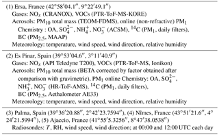
The Es Pinar supersite ($\mathrm{39}{}^{\circ }{\mathrm{53}}^{\prime }{\mathrm{04.6}}^{\prime \prime }$, $\mathrm{3}{}^{\circ }{\mathrm{11}}^{\prime }{\mathrm{40.9}}^{\prime \prime }$) is located on the northeastern part of Mallorca. The monitoring station was placed in the “Es Pinar” military facilities belonging to the Spanish Ministry of Defense. The environment is a non-urbanized area surrounded by pine forested slopes and is one of the most insulated zones on Mallorca, in between the Alcúdia and Pollença bays, but can still be influenced by local anthropogenic emissions. The site is located at an altitude of 20 m a.s.l. The location of the station and a list of available measurements are presented in Fig. 3 and Table 1, respectively.

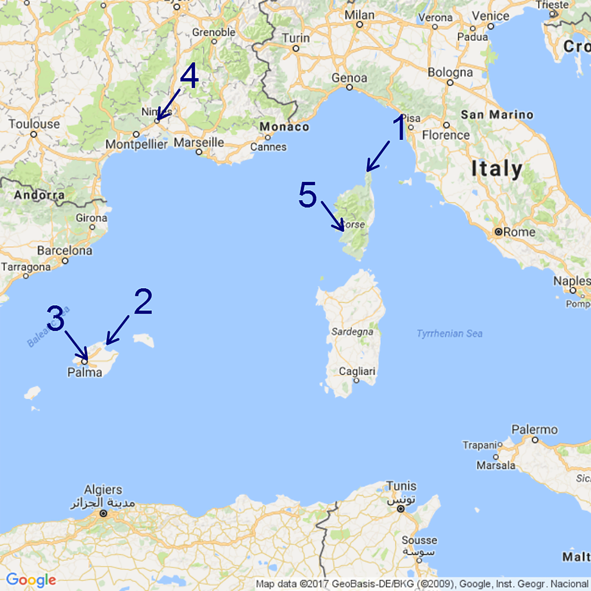
Figure 3 Experimental data sites, including in situ surface stations (1: Ersa, France; 2: Cap Es Pinar, Spain) and meteorological sounding stations (3: Palma, Spain; 4: Nîmes, France; 5: Ajaccio, France). More details about exact location and measurements performed can be found in Table 1.

At Ersa, NO_x (nitrogen oxides) were measured using a CraNOx analyzer using ozone chemiluminescence with a resolution of 5 min. The photolytic converter in the analyzer allows the conversion of direct measurements of NO₂ into NO in a selective way, thus avoiding interferences with other NO_y species. At Es Pinar, an API Teledyne T200 with molybdenum converter was used; therefore, the measurements are not specific to NO₂ and interferences of NO_y are possible for these measurements. VOCs were monitored at both supersites using a proton-transfer-reaction time-of-flight mass spectrometer (PTR-ToF-MS) (Kore^™ second generation at Ersa, and Ionikon^™ PTR-ToF-MS 8000 at Es Pinar). A detailed procedure of VOC quantification is provided in Michoud et al. (2017) for Ersa. Briefly, both instruments were calibrated daily using gas standard calibration bottles and blanks performed by means of a catalytic converter (stainless steel tubing filled with Pt wool held at 350 ^∘C).

A quadruple aerosol chemical speciation monitor (Q-ACSM, Aerodyne Research Inc.; Ng et al., 2011) was used for the measurements of the chemical composition of non-refractory submicron aerosol at Ersa with a time resolution of 30 min. This instrument has the same general structure of an AMS (aerosol mass spectrometer), with the difference that it was developed specifically for long-term monitoring. A high-resolution time-of-flight AMS (HR-ToF-AMS, Aerodyne Research Inc.; Decarlo et al., 2006) operated under standard conditions (i.e., temperature of the vaporizer set at 600 ^∘C, electronic ionization (EI) at 70 eV) was deployed with a temporal resolution of 8 min to determine the bulk chemical composition of the non-refractory fraction of the aerosol for the Es Pinar site. AMS data were processed and analyzed using the HR-ToF-AMS analysis software SQUIRREL (SeQUential Igor data RetRiEvaL) v.1.52L and PIKA (Peak Integration by Key Analysis) v.1.11L for the IGOR Pro software package (Wavemetrics, Inc., Portland, OR, USA). Q-ACSM and AMS source apportionment results discussed in this work are detailed in Michoud et al. (2017). For both sites, source contributions were obtained from PMF analysis (Paatero and Tapper, 1994) of Q-ACSM and AMS OA mass spectra. PMF was solved using the multi-linear engine algorithm (ME-2; Paatero, 1997), using the Source Finder toolkit (SoFi; Canonaco et al., 2013). For the Ersa site, the HOA (hydrocarbon-like organic aerosol) profile was constrained with a reference HOA factor using an a value of 0.1. The a value refers to the extent to which the output HOA factor is allowed to vary from the input HOA reference mass spectra (i.e., 10 % in this case; Canonaco et al., 2013). In such a remote environment, the HOA factor could not be extracted from the OA mass spectral matrix with a classic unconstrained PMF approach. Two other factors were extracted, without any constrains, including SVOOA (semi-volatile oxygenated organic aerosol) and LVOOA (low-volatility oxygenated organic aerosol). For the Es Pinar site, HOA has been constrained using an a value of 0.05. Three additional factors were retrieved, including an SVOOA and two LVOOA factors. In addition to HOA, three other factors have been extracted from the PMF analysis: one SVOOA and two LVOOA factors. Differences between these two LVOOA factors are mainly linked to air mass origins and to the probable influence of marine emissions. For the marine LVOOA factor at both sites, a correlation coefficient (R²) of 0.43 and 0.47 with the main fragment derived from methane sulfonic acid (MSA, fragment ${\mathrm{CH}}_{\mathrm{3}}{\mathrm{SO}}_{\mathrm{2}}^{+}$) was found for Es Pinar and Ersa, respectively. For the sake of clarity and for the purpose of intercomparison with the model outcomes, we merge the two LVOOA factors into one LVOOA for the Cap Es Pinar site to be compared to the Ersa site results. Online aerosol chemical characterization was complemented by an Aethalometer (AE33, MAGEE; Drinovec et al., 2015) at Es Pinar and a multiangle absorption photometer (MAAP5012, Thermo) for the quantification of black carbon (BC) at Ersa. PM₁₀ total mass measurements were taken from TEOM-FDMS (tapered element oscillating microbalance filter dynamic measurement system) at Es Pinar and corrected by a factor obtained after comparison to gravimetric measurements. Finally, daily PM₁ aerosol samples were collected onto 150 mm quartz fiber filters (Tissuquartz, Pall) at both sites. A total of 18 and 8 samples were selected for Ersa and Es Pinar, respectively, for a subsequent analysis of radiocarbon performed on both organic carbon (OC) and EC fractions following the method developed in Zhang et al. (2012).

3.2 Other measurements

For the validation of meteorological parameters, along with the meteorological surface measurements performed at ChArMEx stations, radiosonde data for three stations in the western Mediterranean basin were used for simulation–observation comparisons for meteorological parameters. The radiosondes are performed by Météo France at the two stations of Ajaccio, France ($\mathrm{41}{}^{\circ }{\mathrm{55}}^{\prime }{\mathrm{5}}^{\prime \prime }$, $\mathrm{8}{}^{\circ }{\mathrm{47}}^{\prime }{\mathrm{38}}^{\prime \prime }$), and Nîmes, France ($\mathrm{43}{}^{\circ }{\mathrm{51}}^{\prime }{\mathrm{22}}^{\prime \prime }$, $\mathrm{4}{}^{\circ }{\mathrm{24}}^{\prime }{\mathrm{22}}^{\prime \prime }$), and by AEMet at Palma, Spain ($\mathrm{39}{}^{\circ }{\mathrm{36}}^{\prime }{\mathrm{21}}^{\prime \prime }$, $\mathrm{2}{}^{\circ }{\mathrm{42}}^{\prime }{\mathrm{24}}^{\prime \prime }$). Each day two balloons at about 00:00 and 12:00 UTC are available for each station; a total of 96 balloons are included in the comparisons. Ajaccio and Palma are coastal stations, but Nîmes is farther from the coast compared to the other two stations. Each day two balloons were launched at about 00:00 and 12:00 UTC at each station, and a total of 96 balloons are included in the comparisons for an altitude between the surface and 10 km.

4 Model validation

The CHIMERE model has been previously validated for different parts of the world (Hodzic and Jimenez, 2011; Solazzo et al., 2012; Borrego et al., 2013; Berezin et al., 2013; Petetin et al., 2014; Rea et al., 2015; Konovalov et al., 2015; Mallet et al., 2016). The data set presented in Sect. 3 is used for model validation. First, a representativeness error within simulations is calculated for a list of pollutants, which is necessary to distinguish between uncertainties due to limitations in model resolution and due to other reasons. Then a validation for the meteorological parameters is presented, before comparison of simulation results to gaseous and aerosol measurements.

4.1 Orographic representativeness of Cap Corse simulations

As explained before, during the ChArMEx campaign, an important number of observations were made at Ersa, Cap Corse. In order to use this data set for model evaluation, potential discrepancies due to a crude representation of the complex orography of Cap Corse need to be minimized and quantified since the measurements were performed on the crest line.

For the 10 km domain (D10), we noticed that there was an inconsistency between simulated and real altitude of the cell where the Ersa site is located, altitude being simulated at 360 m a.s.l. below the real altitude of measurements (530 m a.s.l.). Therefore, 1 km horizontally resolved simulations were performed for the inner domain. However, even for the 1 km simulations the simulated altitude remains too low (365 m a.s.l.). This error occurs because the altitude of each cell in CHIMERE is calculated using the average of altitudes of points inside the cell; therefore if the altitude of the ground surface inside a cell happens to vary greatly, the average would be lower than the higher points seen in the cell (which corresponds in our case to the Ersa site located on the crest). In addition, the average of the marine boundary layer height is typically around 500 m (Stull, 1988); therefore a discrepancy in the simulated altitude could cause significant errors in the simulations. These two reasons make it important to explore the representativeness of the simulations regarding this station.

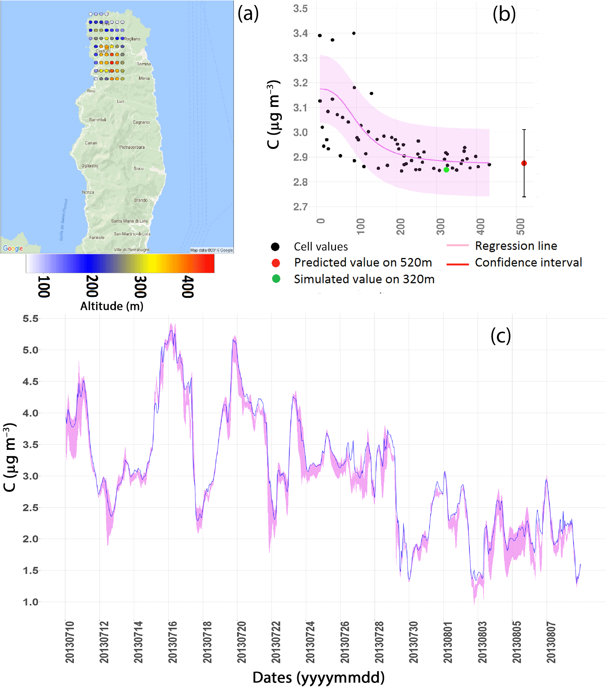
Figure 4 Orographic representativeness error. (a) Neighboring cells used in the orographic representativeness test; (b) an example of nonlinear regressions performed on one time step for organic aerosol (OA, one point corresponds to one grid cell); (c) results from all hourly simulations for OA. In (b) and (c), the purple ribbon shows the confidence interval of the regression results. In (c), the blue line shows the simulations at the nominal Ersa site grid cell.

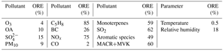
This led us to perform an orographic representativeness test on the 1 km domain (D1) at the Ersa site. A matrix of neighboring cells around the grid cell covering the Ersa station (up to 5 km distance) was taken (Fig. 4a), and species concentrations were plotted against the variation of the altitude of these different cells. The highest altitude reached by one of the cells is about 450 m. Then, the concentration on the exact altitude (530 m) was extrapolated using a nonlinear regression between the altitude and the concentration of the selected cells with several different equations for each time step. In total, nine nonlinear equations were tested, among which only five were finally used for the calculation of the representativeness error. For the other four equations, convergence problems occurred and no stable solution could be found for some of the hourly time steps (see Supplement Sect. SI3 for details). Regressions were performed separately for each of the 720 hourly time steps of the 1-month simulations. An example of this regression for OAs for one time step and one of the equations is shown in Fig. 4b (Eq. 1 from SI3). The results were filtered using two criteria (convergence of regression for each time step and a correlation coefficient between fitted and simulated points of higher than a threshold) depending on statistical values of the regressions (see Supplement Sect. SI3 for details) and only regressions conforming to these criteria were retained. If at least two converging regressions were not retained for a given time step, the results for that time step were not further used. Figure 4c shows the compiled results for all equations and all simulation times in one time series for total OA concentration. Note that model output was generated with an hourly time step. Using these results, for a list of different species, an orographic representativeness error was calculated using the average of the difference of the upper and lower confidence intervals for all equations. As an example, carbon monoxide, which is a well-mixed and a more stable component in the atmosphere, presents the lowest error among the tested species (2 %). Ozone also presents one of the lowest errors (4 %) and nitrogen oxides one of the highest (75 %). OA, of particular interest for this study, shows a moderate error of 10 %. In terms of meteorological parameters, relative humidity appears more affected (relative orographic representativeness error of 18 %) than temperature (the relative orographic representativeness error is calculated on values of T in ^∘C). A summary of results of this test is shown in Table 2.

Table 2 Calculated relative orographic representativeness error (ORE) for a list of species and meteorological parameters. MACR+MVK presents the sum of methyl vinyl ketone and methacrolein.

A general conclusion is that secondary pollutants with higher atmospheric lifetimes appear to be well represented from a geographic point of view. Conversely, model–observation comparisons for more reactive primary and secondary pollutants with short lifetimes (primary such as NO_x and reactive secondary such as methyl vinyl ketone and methacrolein, MVK+MACR) should be performed with caution keeping in mind the fact that the simulated altitude is not representative of the orography for this specific station. This is due to the fact that short-lived primary species have not yet had the chance to vertically mix, if emission sources happen to be nearby (which is the case here). Vertical layering of these concentrations then results in significant sensitivity to the simulated altitude of a site. Conversely, secondary species, which have partly been transported from the continental boundary layer, are believed to be better mixed vertically. For those species, differences in the simulated versus observed altitude lead to relatively smaller errors.

The question of which domain should be used for model–measurement comparisons remains. As seen above, D10, despite having a sufficiently fine resolution for most continental areas, is not capable of representing the complex orography of Cap Corse; therefore the D1 simulation results have been used for comparisons, except for meteorological parameters, where all possible domains (and resolutions) are compared. The Es Pinar station does not have the same intense altitudinal gradient seen at Ersa; therefore the aforementioned test was not performed for this station and the D10 simulations are used for comparisons for Es Pinar.

In the following section, the confidence intervals representing the orographic representativeness error derived in this section are considered for the model–observation comparisons.

4.2 Meteorology evaluation

Meteorological output of the mesoscale WRF model at different resolutions has been used as input to the CHIMERE CTM. The meteorological data used by CHIMERE were compared to various meteorological observations such as radiosondes and surface observations at the measurement sites. Detailed results of these comparisons are given in the Supplement (Sect. SI4). Here, a short overview of the results and the implications for the model ability to simulate transport to the measurement sites is given.

Comparisons for temperature, a basic variable to control the quality of meteorological simulations, show a good correlation for radiosonde comparisons (typically from 0.60 to 0.85 for hourly values) and a low bias (typically from −1.16 to −0.39 ^∘C) for the three sites of Palma, Nîmes, and Ajaccio. Wind speed shows a good correlation at higher altitudes, and also near the surface for Nîmes and Palma for radiosonde stations, while for the Ajaccio station the sea–land breezes are probably not well represented in the model. For Es Pinar, the coastal feature of the site is difficult to take into account in a 10 km horizontally resolved simulation and leads to larger errors. Ground-based meteorological measurements were also compared at both sites (SI4). At Ersa, the correlation in finer domains is better than that of D10 for wind speed (typically around 0.66 versus around 0.60). For the E-OBS network (surface data sets provided by European Climate Assessment and Dataset, ECAD) project for monitoring and analyzing climate extremes, (Haylock et al., 2008; Hofstra et al., 2009) comparisons (SI4) also show a good correlation and a low bias for temperature (correlation of 0.79 with a bias of −0.54 ^∘C for mean temperature observed for 71 stations in D10 domain), while the daily minima seem to be underestimated (bias of −3 ^∘C observed for 71 stations).

While the general comparison between the hourly meteorological fields used as input for CHIMERE simulations and observations is in general already satisfying, the correlation becomes higher and the bias lower when daily averages representative for different meteorological conditions are compared instead of hourly values.

4.3 Gaseous species

Among all the gaseous species available in the observations, four were chosen in this study: nitrogen oxides (NO_x), isoprene (C₅H₈), monoterpenes, and the sum of methacrolein and methyl vinyl ketone (hereafter called MACR+MVK). These four species were chosen since isoprene and monoterpenes are the principal precursors for biogenic SOA, MACR+MVK are formed during isoprene oxidation, and NO_x is a good tracer for local pollution. The comparisons for the Ersa and Es Pinar stations are shown in Fig. 5, and statistics of the comparison are shown in Table 3. For Ersa, the orographic representativeness errors derived in Sect. 4.1 are also shown. In all comparisons, the results for the simulations with the modified VBS scheme are used, but the choice of the OA scheme only slightly affects the simulation of gaseous species (mainly via heterogeneous reactions on aerosol surfaces included within CHIMERE).

Table 3 Statistical data for time series shown in Fig. 5; Mean_obs shows the average of observations. Values in parentheses for Es Pinar NO_x statistics show the comparison of NO_y simulations to NO_x measurements.

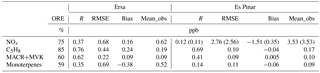
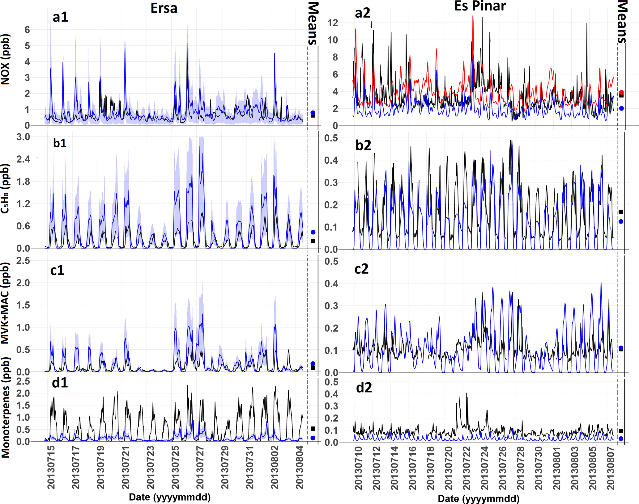
Figure 5 Time series showing the comparison of simulated (in blue) and measured (in black) gaseous species during the ChArMEx/SAFMED campaign period. (a) Nitrogen oxides (time series in red for Es Pinar represents NO_y concentrations); (b) isoprene; (c) MACR+MVK (methyl vinyl ketone+methacrolein); (d) monoterpenes. Statistical data for these comparisons are given in Table 2. The ribbon around Ersa simulations presents the orographic representativeness error. On the right side of each time series, two points are shown presenting the average of simulations (blue circle) and observations (black square).

Results show that there is a good correspondence between the averages of simulated and observed nitrogen oxides at Ersa (Fig. 5a1). The low correlation for nitrogen oxides at Ersa might be partly explained by the high representativeness error (75 %) for this component. This is because the altitude in the simulations is lower and therefore the emission sources are closer in the model than they are in reality. At Es Pinar (Fig. 5a2), since the measurements are not specific to NO₂, the NO_y time series are added to the figure as well. As a consequence, if the model had no error, the NO_x observations would be expected to lie between NO_x and NO_y simulations. This is the case because NO_x observations are on average 40 % higher than the NO_x simulations and 9 % lower than the NO_y simulations.

For isoprene (Fig. 5b1 and b2), a good correlation (0.76, 0.71) between simulations and observations appears at both sites. However there is an important overestimation (by a factor of 2.5) in the simulations for the Ersa site, which could also be linked to the high orographic representativeness error (85 %), and also to the fact that local emissions sources may not be correctly taken into account in the MEGAN emission model. Conversely, at Es Pinar isoprene is underestimated by about 25 %. The sum of MACR+MVK (Fig. 5c1 and c2) is overestimated by about a factor of 2 at Ersa, following the pattern of overestimation of isoprene at this site, while the bias is small at Es Pinar. Monoterpenes (Fig. 5d1 and d2) show an underestimation by about 70 % at both sites, observations being about 5 times larger at Ersa than at Es Pinar. Again, this could be related to the orographic representativeness error at Ersa and to local vegetation that was not accounted for at both sites.

Daily correlations of 0.35, 0.87, 0.85, and 0.58 (instead of 0.37, 0.76, 0.62, and 0.35 hourly values) are seen at Ersa for nitrogen oxides, isoprene, MACR+MVK, and monoterpenes, respectively. These values change to 0.16, 0.51, 0.72, and 0.10 for daily comparisons (instead of 0.12, 0.69, 0.41, and 0.14 when correlating hourly values) at Es Pinar. Improvements in correlation for daily averages could be related to those in meteorological parameters, at least for Ersa. They show the difficulty to correctly simulate short-term (hourly) variations both in meteorological parameters and chemical species.

A drawback of the comparisons for isoprene, and monoterpenes, contributing respectively to 40 and 60 % of SOA simulated with the modified VBS scheme in the western Mediterranean region, is the measurements' representativeness restricted to local scales. A more regional evaluation of these precursor species would have been necessary since SOA simulated and observed at Ersa and El Pinar was partly formed far away from these sites.

As mentioned before (Sect. 2), isoprene and terpene emissions in our work are generated by the MEGAN model (Guenther et al., 2006). Zare et al. (2012) evaluated isoprene emissions derived from the MEGAN model coupled to the hemispheric DEHM CTM against measurements. On average over 2006, they found a simulated isoprene overestimation at four European sites (between a factor of 2 and 10), good agreement (within ±30 %) at two sites, and an underestimation at two sites (also between factors of 2 and 10). However, none of the sites were located close to the Mediterranean Sea. Curci et al. (2010) performed an inverse modeling study to correct European summer (May to September) 2005 MEGAN isoprene emissions from formaldehyde vertical column OMI measurements (given that isoprene is a major formaldehyde precursor). For the western Mediterranean area, they found an isoprene emissions underestimation using MEGAN of 40 % over Spain, a tendency for an underestimation but with regional differences over Italy, and only small differences over France. This comparison globally lends confidence to MEGAN-derived isoprene emissions. Unfortunately, to our best knowledge, no comparable studies exist in order to validate monoterpene emissions. For the Rome area in Italy, Fares et al. (2013) concluded for a variety of typical Mediterranean tree and vegetation species mix, that MEGAN correctly simulated (within 10 % error) mean observed monoterpene fluxes over the last 2 weeks of August 2007 for a variety of Mediterranean tree and vegetation species mix, as long as a canopy model was included (as in our study).

4.4 Particulate species

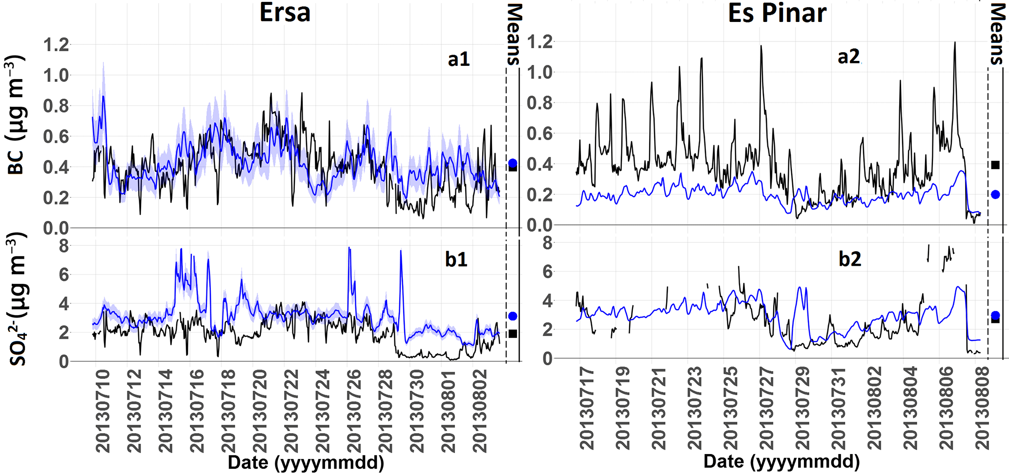
Figure 6 As for Fig.  5, but for particulate matter. (a) Black carbon (BC); (b) sulfate particles. Statistical data for these comparisons are given in Table 4.

Table 4 Statistical data for time series shown in Fig. 6; Mean_obs column shows the average of observations.

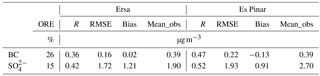
Figure 6 shows the comparison between observations and simulations for particulate sulfate and BC in PM₁. These two species are chosen as two important fine aerosol components, before the comparison of OA in Sect. 5. The left panel shows the comparison for Ersa and the right one for Es Pinar. Statistical information for these species is given in Table 4. There is an overestimation for sulfate particles (Fig. 6b1 and b2) by about 45 %, well beyond the representativeness error for this species (15 %). In addition, the short and sharp decreases in the measurements of sulfates correspond to low clouds passing at the level of the station, which are not simulated by the model. Cloud scavenging processes are already taken into account in the model. However, because of the unique geographical characteristics mentioned before for this site, the meteorological inputs did not simulate these fog events and therefore cloud scavenging was not activated in the simulation. Since these decreases concern only a small percentage of the observations, they do not have a major effect on the outcome of these comparisons. While this effect is very visible for sulfates, it is less pronounced for other particulate species such as BC and OA. A large sulfate peak simulated in the morning of 29 July is not present in the observations; it originates in the model from an air mass arriving from Marseille, which is both a busy harbor and an important industrial area with large SO₂ emissions. This is probably due to small errors in the wind fields. In addition, there are two periods of overestimation of this species in the simulations: the period of 18 to 20 July and the period of 29 July to the night of 1 August. During the second period, the ACSM PM₁ observations show concentrations of close to zero, which are consistent with PM₁₀ particle-into-liquid sampler ion chromatography (PILS-IC) sulfate measurements. For this period elevated southerly winds are observed in the Corsica area, and the absence of strong SO₂ sources in this sector might explain the lower concentrations that are seen not only for sulfate but also for BC. The constant overestimation of sulfates during this period may suggest an overestimation of boundary conditions for these species.

A moderate correlation (0.36) between the model and the observations is seen for BC (Fig. 6a1 and a2), but the representativeness error is important for this species (26 %), since one of its primary origins is emission of ships passing nearby the coasts of Cap Corse. The local emissions due to shipping activities at Ersa and anthropogenic activities at Es Pinar are visible in the observations as frequent narrow (in time) peaks. These activities are also visible in the simulations at Ersa. However, at Es Pinar the model does not succeed in simulating them, as already observed to an even larger extent for NO_x. The slight overestimation of BC (5 %) in the model for the Ersa site could be explained by the orographic representativeness error. The same cloud effect seen for the sulfate particles at Ersa is visible to a lesser extent for BC for the Ersa site as well. Correlation between daily observations and the simulations was also calculated. R² is 0.51 and 0.56 for the Ersa station (instead of 0.36 and 0.42 for hourly values) and 0.81 and 0.65 for the Es Pinar station (instead of 0.47 and 0.52 for hourly values) for sulfate and BC, respectively. Similar to meteorological parameters, the model can reproduce the daily concentration changes for these two species better than the hourly changes.

5 Organic aerosol simulation

A description of each of the four schemes for the simulation of OAs tested within the CHIMERE model for the Mediterranean area has been given in Sect. 2. These four schemes are the CHIMERE standard scheme, the VBS scheme with BSOA aging (noted as Standard VBS_ba), the VBS scheme without BSOA aging (noted as Standard VBS_nba), and the modified VBS (noted as modified VBS) scheme, which includes fragmentation and formation of nonvolatile OA. For each scheme, four domains were used: one coarse domain and three others nested inside the coarse one with increasing resolutions. As before, the simulations from the finest domain are used for the comparisons. The domain with the finest resolution (1 km) was used for the representativeness tests. For each scheme, meteorological and boundary conditions are the same; hence only the simulation of OAs and subsequently the aggregation of anthropogenic PM emissions differ among simulations.

5.1 Comparison of PM₁ total organic aerosols concentration

Figure 7 Compared time series of total PM₁ organic aerosol (OA) concentration at Ersa (top) and Es Pinar (bottom) – black: observations; green: modified VBS; brown: standard VBS without BSOA (biogenic secondary organic aerosol) aging; blue: CHIMERE standard; red: standard VBS with BSOA aging. For each site the average of simulations is shown with circles in corresponding colors and the observations with black squares. Shaded area for Ersa presents the orographic representativeness error. Statistical data are shown in Table 5.

Table 5 Statistical data for hourly time series shown in Fig. 7. R is the correlation coefficient between model and measurements, RMSE is the root mean square error, mean_sim and mean_obs show the average, and SD_sim and SD_obs show the standard deviation of simulations and observations, respectively.

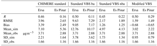
Figure 7 shows the time series of comparison of OAs for these four schemes with the measurements at Ersa and Es Pinar. The circles beside each plot show the average concentration for different time series; in addition Table 5 shows the statistical parameters corresponding to these time series. The observed OA concentration at the Ersa site measured by the ACSM in the PM₁ fraction has an average of 3.71 µg m⁻³ and that of the Es Pinar site measured by the AMS in the PM₁ fraction a somewhat lower average of 2.88 µg m⁻³. The difference between the two sites may be attributed to the fact that Cap Corse is closer to both local and transported (continental) biogenic sources than Es Pinar. The VBS scheme with BSOA aging greatly overestimates the OA with a bias of more than a factor of 3. As mentioned before, the aging of biogenic aerosols in the VBS scheme usually results in an overestimation in OAs (Lane et al., 2008). With the BSOA aging option turned off, the standard VBS scheme comes much closer to the average of total OA concentration measured at both sites (relative biases of below 50 %). The CHIMERE standard scheme also overestimates the mass concentration of OAs, but to a lesser extent compared to the VBS scheme with BSOA aging (bias of a bit less than a factor of 2). The modified VBS scheme corresponds much better to observations (negative biases about 20 %). The model results agree for both stations in this regard. At Ersa, biases of +244, +91, +34, and −18 %, respectively, are observed for the VBS standard scheme with BSOA aging, the CHIMERE scheme, the standard VBS scheme without BSOA aging, and the VBS modified scheme. The corresponding numbers are of +218, +98, +43, and −23 % for Es Pinar.

The daily correlation for the modified VBS scheme is 0.63 and 0.51 for Ersa and Es Pinar, respectively (instead of 0.50 and 0.29 for hourly values). This shows, again, that the model represents day-to-day changes better than hourly variations. While the concentrations of both the modified VBS scheme and the standard VBS scheme without BSOA aging correspond well with the experimental data, other aspects such as origins of the formed OA and its oxidation state have to be considered before reaching any conclusion about the robustness of these schemes.

The overestimation of secondary OA with the CHIMERE standard scheme is a new feature, not apparent in previous studies (Bessagnet et al., 2008; Hodzic and Jimenez, 2011; Petetin et al., 2014). A previous comparison of CHIMERE with OA simulations using the same scheme and coupled to MEGAN biogenic emissions resulted in a good comparison or underestimation with OC observations over Europe from the CARBOSOL project (Gelencsér et al., 2007) for summer 2003, when biogenic SOA was dominant. However, this comparison included only one site close to the western Mediterranean basin (Montelibretti, Italy). The overestimation of BSOA in the VBS scheme when the BSOA aging is activated was documented for the USA on several occasions (Robinson et al., 2007; Lane et al., 2008). Ultimately, it cannot be excluded that the OA overestimation with both schemes at Ersa and Es Pinar is also due to biogenic VOC (BVOC) overestimation. However, the available material does not support this hypothesis: (i) OA overestimation is observed at two independent, distant sites, (ii) local monoterpene underestimation is observed at both these sites, and (iii) no evidence for MEGAN monoterpene overestimation is available in literature and MEGAN isoprene overestimation over the western Mediterranean area was ruled out by satellite observations (Curci et al., 2010).

5.2 Total carbonaceous particle origins based on ¹⁴C measurements

The results of ¹⁴C measurements in carbonaceous aerosol filter samples for the PM₁ fraction at the Ersa and Es Pinar sites were used in order to better discriminate between the modern and mostly biogenic versus fossil and anthropogenic origin of OAs, and to compare it to simulations with different OA schemes tested. It must be noted that in the simulations, species are not separated automatically into fossil and nonfossil parts; therefore these fractions need to be calculated as a posttreatment of simulations, affecting each relevant particulate species to both fractions. ASOA is considered to be in the fossil fraction and BSOA in the nonfossil fraction. For carbonaceous aerosol, residential or domestic uses are considered as nonfossil as they are mostly related to wood burning (Sasser et al., 2012). Therefore, they are attributed to the nonfossil bin (3.6 % for BC and 12.3 % for OC; Sasser et al., 2012). The nonfossil contribution of ASOA and primary OA (POA) due to biofuel usage is ignored here, as it is minor (< 5 %). No major biomass burning events were seen in the period of this study, but minor contributions of this source cannot be excluded. It should also be mentioned that the ¹⁴C measurements show the mass of carbonaceous particles in each filter and therefore have a unit of µgC m⁻³, while the simulations show the total OAs in µg m⁻³. In the comparisons that follow, it is pertinent to use an organic matter (OM) ∕ OC conversion factor to be able to compare the ¹⁴C measurements to simulations. For this purpose, an average OM ∕ OC factor of 2 is used for the secondary aerosol fraction (both for the LVOOA and SVOOA factors), while a factor of 1.3 is used for HOA according to Aiken et al. (2008). However, the choice of the OM ∕ OC factor has a small effect on the outcome of general comparisons since HOA values are marginal compared to other factors and we are only interested in the relative contribution of fossil and nonfossil factors.

Figure 8a for Ersa and 8b for Es Pinar show the average of all filters for each scheme compared to the observations, while Fig. 9a and b show the relative distribution of fossil and nonfossil sources at both sites. Among these total averages, the distribution at Ersa is 81 % ± 1.5 % nonfossil and 19 % ± 1.5 % fossil, and 67 % ± 3 % nonfossil versus 33 % ± 3 % fossil at Es Pinar. Apparently, biogenic contributions to OA are dominant at both sites, but larger for the Ersa site.

Figure 8 Comparison of simulations to ¹⁴C measurements – (a) comparison of filters to four schemes for Ersa; (b) comparison of filters to four schemes for Es Pinar. For both figures from outer ring to inner ring: observations, modified VBS, standard VBS with BSOA (biogenic secondary organic aerosol) aging, standard VBS without BSOA aging, and CHIMERE standard scheme.

While the comparison of averages for all schemes with Ersa measurements shows that the modified VBS scheme is the closest in fossil and nonfossil partitioning (19 %∕81 % ± 1 %), the CHIMERE standard scheme also performs well when looking at the percentage of distribution for each source (20 %∕80 % ± 1 %). The VBS scheme with BSOA aging shows an underestimation in the percentage of fossil carbons (16 %∕84 % ±  0.7 %), which can be due to the overestimation of biogenic aging of SOAs in this scheme; conversely, the VBS scheme without BSOA aging shows an important overestimation of the fossil percentage (34 %∕66 % ± 2 %).

A distribution of 33 %∕67 % ± 3 % of the fossil and nonfossil fractions is observed at Es Pinar. As for the Ersa site, the modified VBS scheme is the closest to the observations (32 %∕68 % ± 2.5 %). The CHIMERE standard scheme shows an underestimation of the fossil contribution with a distribution of 28 %∕72 % ± 3 %. The standard VBS scheme with BSOA aging underestimates the fossil contribution with a distribution of 21 %∕79 % ± 1.5 %, while the standard VBS scheme without BSOA aging largely overestimates the fossil contribution (42 %∕58 % ± 2 %). These results show that the two sites differ greatly when taking into account nearby sources and geographical conditions; the Ersa site is an elevated rural station at the interface between the marine boundary layer and the residual boundary layer, and the Es Pinar site is a seaside station closer to anthropogenic sources. These differences should normally be represented in the percentage of fossil carbon concentrations in both observations and simulations. Although this difference is noticeable in observations, and also in the modified VBS scheme, it is less emphasized in the CHIMERE standard scheme and in the VBS standard scheme with either parameterization of aging.

A more detailed look at individual filters for the modified VBS scheme for the Ersa and Es Pinar sites is presented in Fig. 9a and b, respectively. The tendencies from one day to another are in most cases not reproduced correctly for both sites. Therefore while the average mass repartition of modern and fossil sources is well represented by this scheme, the day-to-day variability is not fully consistent with the measurements. This inconsistency is also seen in the other tested schemes.

Figure 9 Comparison of simulations to ¹⁴C measurements – (a) Ersa individual filters; (b) Es Pinar individual filters. For each filter, measurements are on the left and modified VBS simulations are on the right. Dark or light brown shows fossil and dark or light green shows nonfossil sources.

5.3 Volatility and oxidation state comparison with PMF results

The PMF results of the ACSM/AMS measurements give us the chance to learn more about the oxidation state of the OAs (Michoud et al., 2017, for Ersa). The PMF analysis allows us to divide PM₁ OA measurements into different groups with distinctive mass spectra corresponding to distinctive oxidation state (Lanz et al., 2010). The most common retrieved factors of such an analysis are HOA, SVOOA, and LVOOA. However, it does not give direct information about the volatility distribution of each group. This makes the PMF output difficult to compare with our model results, which give the volatility distribution of OA but not its oxidative state. Here, we first compare volatility distributions obtained with the four aerosol schemes, and then try to attribute the simulated aerosol to the three factors HOA, SVOOA, and LVOOA, in order to compare it to the observed distributions. The three schemes based on the VBS scheme already distribute aerosols in volatility bins (Robinson et al., 2007). The distribution to LVOOA and SVOOA for these three schemes was performed mainly by taking into account the saturation concentration, with the threshold chosen as a saturation concentration C^* ≥ 1 µg m⁻³ for SVOOA and C^* ≤ 0.1 µg m⁻³ for LVOOA (Donahue et al., 2012). Primary OAs were considered to be in the HOA factor regardless of their saturation concentration. For the CHIMERE standard scheme, each surrogate species is associated with a saturation vapor pressure, which was used to calculate the saturation concentration for each component at ambient temperature.

The observations show that at Ersa, the LVOOA factor dominates the PMF results (88 %), with 10 % SVOOA and a minor (only 2 %) contribution of HOA. For the Es Pinar site the contribution of LVOOA drops to 75 % and the contribution of SVOOA and HOA becomes somewhat larger (21 % and 4 %, respectively). As mentioned before, the Es Pinar site is more influenced by local anthropogenic sources. Therefore, more local OA emissions are expected, which corresponds to the increase in the HOA percentage seen in the observations. These emissions are oxidized locally to form SVOCs that fall in the SVOOA group, explaining the rise in the percentage of this group.

Figure 10a and b show the relative distribution of all OAs in seven volatility bins for all tested schemes for the Ersa and Es Pinar sites, respectively, and for all tested schemes. For each scheme, the average for the total period of the simulations was used to calculate the percentage in each bin. The bins shown are in the range of 10⁻³–10³ µg m⁻³; all the aerosols with a volatility higher or lower than the extremes are put in the last high or low bin, respectively.

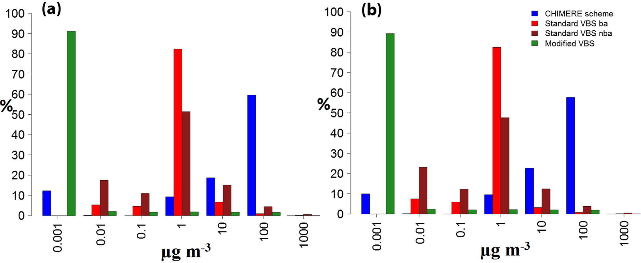
Figure 10 Distribution of simulated organic aerosol (OA) in volatility bins – (a) Ersa volatility bins; (b) Es Pinar volatility bins.

These figures show that the percentage of aerosols in each volatility bin for the two different sites is relatively similar. The CHIMERE standard scheme distributes most of the aerosol in the three bins in 1–100 µg m⁻³ volatility ranges, which falls into the SVOOA group obtained with PMF. This is due to the initial distribution of volatilities of surrogate SVOC species used that best fit chamber measurements, and the fact that there is no aging mechanism in this scheme to make the aerosols less volatile. The 100 µg m⁻³ volatility bin corresponds to SVOCs produced from isoprene and monoterpene oxidation and presents the highest percentage for this scheme. The standard scheme also produces 16 % of OAs in the LVOOA range (volatilities corresponding to a C^* between 0.001 and 0.1 µg m⁻³). The standard VBS scheme with BSOA aging has only a small fraction of aerosol in the LVOOA range (from SVOC emission aging) since, by construction of the scheme, the most aged BSOA and ASOA aerosols fall in the 1 µg m⁻³ volatility bin, which is actually the bin with the highest percentage of OA. The standard VBS scheme without BSOA aging presents relatively similar results to the scheme with biogenic aging, with as expected larger percentages for higher volatilities in the absence of aging. It also shows a larger LVOOA fraction, probably because the lower total OA concentration favors the contribution of lower-volatility SVOCs to the aerosol phase. On the whole, the two schemes yield much too low LVOOA fractions as compared to observations. The modified VBS scheme has a more realistic distribution into the three oxidation groups. In this scheme, the highest percentage of OA falls in the 10⁻³ µg m⁻³ volatility bin, which is in the LVOOA range. The rest of the aerosols are distributed almost equally in volatility bins between 10⁻² and 10² µg m⁻³ with a slight decrease in percentage in the higher-volatility bins. The percentage in higher-volatility bins at Ersa are slightly lower than the ones at Es Pinar, which could be explained by the stronger local sources at the Es Pinar site with stronger primary SVOC emissions.

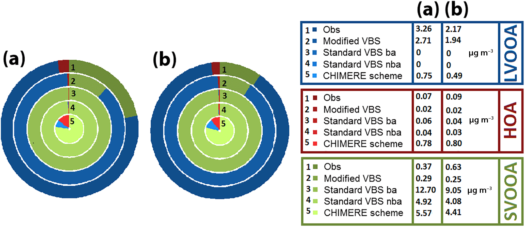
Figure 11 Comparison to PMF results – (a) comparison of observed PMF factors to those derived from four schemes for Ersa and (b) for Es Pinar. For both figures from outer ring to inner ring: observations, modified VBS, standard VBS with BSOA aging, standard VBS without BSOA (biogenic secondary organic aerosol) aging, and CHIMERE standard scheme. LVOOA refers to low-volatility oxidized organic aerosol, SVOOA to semi-volatile oxidized organic aerosol, and HOA to hydrocarbon-like organic aerosol.

Figure 11a and b show the calculated HOA, LVOOA, and SVOOA groups in simulations compared to the ones in observations at Ersa and at Es Pinar, respectively. At Ersa, the results of the modified VBS scheme are consistent with the observations with a slight underestimation of HOAs, which is more visible at Es Pinar. The standard CHIMERE scheme leads to higher, overestimated HOA values, as primary OA emissions are considered nonvolatile. Only the modified VBS scheme succeeds in reproducing the major contribution of LVOOAs at both sites. However, while staying close to observations at Ersa, it seems to overestimate the formation of LVOOAs at Es Pinar. The standard VBS schemes with or without BSOA aging greatly underestimate the formation of LVOOAs, and as a counterpart overestimate the formation of SVOOAs. Therefore, among the tested schemes, only the modified VBS scheme allows us to represent the distribution of the different PMF factors in a satisfying way.

6 Budget of organic aerosols

In Sect. 5, we have highlighted the best performance of the modified VBS scheme for OA simulation amongst the tested schemes by comparison to observational data at two different sites in the western Mediterranean basin. In the present section, we use this scheme in order to simulate the OA distribution and its anthropogenic and biogenic origins over the western Mediterranean basin during the SAFMED campaign.

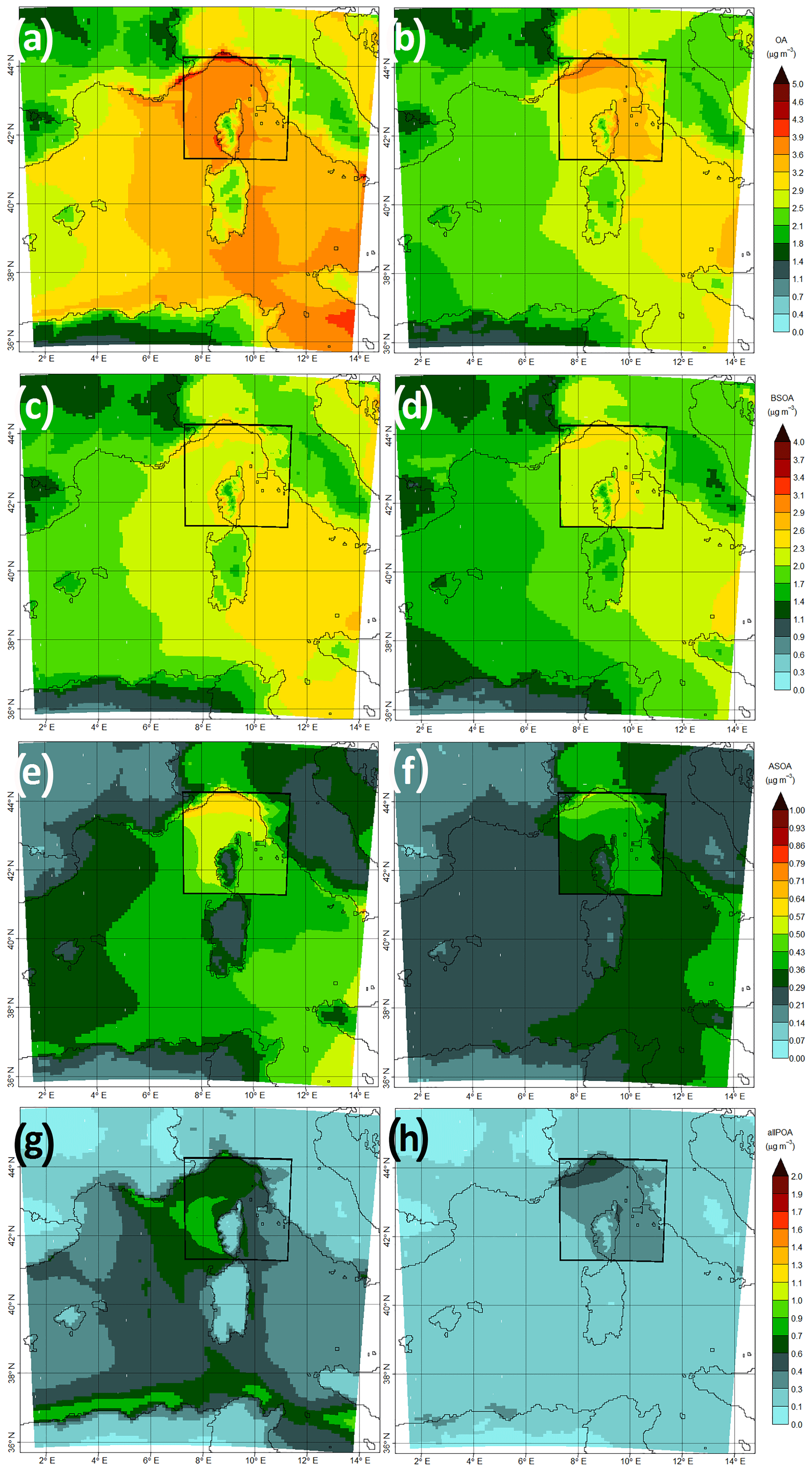
Figure 12 Average organic aerosol (OA) concentrations over the western Mediterranean basin simulated from 10 July to 9 August 2013 with the modified VBS scheme. The left column is near the surface, and the right column is for an altitude between 300 and 450 m a.s.l. From top to bottom: (a–b) total organic aerosol concentration (µg m⁻³); (c–d) BSOA (biogenic secondary OA) concentration (µg m⁻³); (e–f) total ASOA (anthropogenic secondary OA) concentration (µg m⁻³); (g–h) sum of POA (primary OA) and its subsequent oxidation products (µg m⁻³). Results are from the D3 simulation (3 km horizontal resolution) within the framed area and from the D10 simulation outside the framed area (10 km resolution).

Figure 12 shows a series of figures in which the left column always corresponds to simulations near the surface, and the right column shows the same concentration at an altitude of between 300 and 450 m (for marine grid cells; called for simplicity boundary layer, BL). Each row shows a different component, with the first row corresponding to OA concentrations, second row to biogenic OA concentrations, and third row to anthropogenic OA concentrations; the last row presents the sum of POA and all its subsequent oxidation products. The larger part of each figure corresponds to D10 simulations, while the part inside the black rectangle shows the D3 simulations, both showing the average of the OAs for the whole simulation period (1 month from 10 July to 9 August). Figure 13 shows the same type of figures for the percentage of contribution of biogenic OAs, anthropogenic OAs, and the sum of POAs (that is POA and POA oxidation products). The small differences at the interface of the two domains is because the CHIMERE model is a one-way chemistry–transport model: the simulations for the parent domain influence the simulations for the nested domain; however, the inverse is not applied; therefore any concentrations observed in the nested domain will not change the concentrations seen in the parent domain.

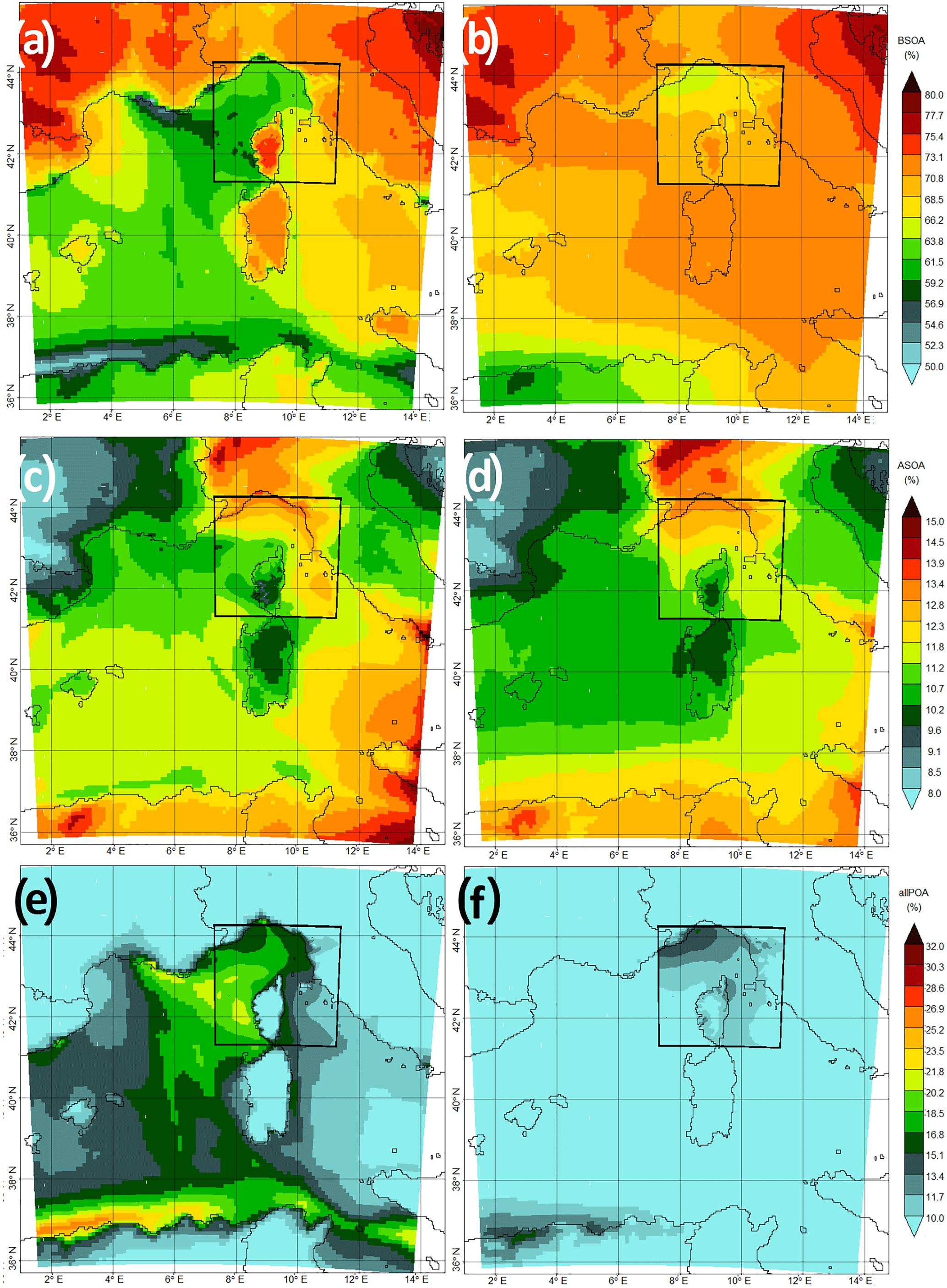
Figure 13 As Fig. 12 but for relative contributions of BSOA, ASOA, and POA to total OA (%). From top to bottom: (a–b) biogenic secondary organic aerosol (BSOA); (c–d) anthropogenic secondary organic aerosol (ASOA); (e–f) POA and its subsequent oxidation products.

Examining figures corresponding to OA concentrations (Fig. 12a and b), at the surface level there is a region of high concentration of OA in the Gulf of Genoa (between Genoa and Corsica) reaching nearly 4 µg m⁻³. The high concentration in this area is less pronounced in the BL (Fig. 12b). The concentration of biogenic OAs (Fig. 12c and d) is high over the basin as well as over Europe, and less important over North Africa. The percentage of contribution of this type of aerosol to the overall OA concentration is shown in Fig. 13a and b. As expected from looking at the total concentration of biogenic OAs, their contribution stays on average around 70 % over the basin, but is lower in the Gulf of Genoa (about 60 % at surface, nearly 70 % at altitude). In this area the secondary anthropogenic OAs show a bit higher contributions compared to their contribution to the rest of the domain (around 14 % instead of 12 %); also, the contribution of POAs (and their subsequent oxidations) is also quite high in this region (around 20 %). The areas between Corsica and Marseilles and also the northern coast of Africa are main shipping routes in the western Mediterranean basin, with high amounts of shipping related emissions. They affect POA and its semi-volatile oxidation products as shown in Fig. 12g and h, with concentrations as high as 0.9 µg m⁻³ around Corsica and near the African coast. This corresponds to a contribution of around 22 % over Corsica and 25 % over the coast of Africa (Fig. 13e and f). These values may actually be upper limits since shipping primary SVOC and IVOC emissions were treated as those from other activity sectors (see Sect. 2.2.3), and recent chamber study data suggest lower SOA yields from shipping emissions (Pieber et al., 2016) than are used here. The influence of shipping emissions is not visible in the BL because vertical mixing within the marine boundary layer is weak, thus in the 300 to 400 m layer the contribution of biogenic OA becomes dominant for the whole basin. Still, in the Gulf of Genoa, some effects of anthropogenic influences are visible in the BL, which could be linked to emissions originating from industrial sites and the harbor of Genoa area, which are apparently better mixed vertically over the continental convective boundary layer (in the coastal region with strong orography). These anthropogenic emissions are visible in figures corresponding to anthropogenic OA, formed from anthropogenic VOCs and especially aromatic compounds (Fig. 12e and f for absolute concentrations and Fig. 13c and d for relative percentages). While the average concentration of anthropogenic OAs stay relatively low over the western Mediterranean basin (an average of 0.30 µg m⁻³ near the surface), they become more pronounced around the Gulf of Genoa and the eastern part of the domain both near the surface and in the BL. A contribution of about 12–15 % both near the surface and in the BL is seen for this component above the Gulf of Genoa and over the highly industrialized and densely populated Po Valley.

7 Conclusion and discussion

Three schemes for the simulation of OA were implemented and tested along with the standard scheme in the CHIMERE chemistry–transport model. The simulations from each of the four schemes were compared to detailed experimental data obtained from two different stations in the western Mediterranean area during the ChArMEx campaign in summer 2013. The simulations were performed over 1 month in the summer of 2013 on four nested domains with increasing resolutions, the largest one covering Europe and northern Africa with a 30 km horizontal resolution, to the smallest one focused on the Cap Corse area with a 1 km horizontal resolution.

For the comparisons of OA simulated with different schemes to observations, we explored three different aspects: mass concentration, distribution with respect to volatility and oxidative state of OA classes derived using PMF, and ¹⁴C measurements discriminating fossil or nonfossil origin. Results show that the modified VBS scheme (i.e., including the fragmentation and formation of nonvolatile OAs), better corresponds to the observations at both sites, and this for all three aspects. The modified VBS scheme succeeds at simulating the average concentration of OA for the 1-month campaign period with low bias (about −20 % at both sites), even if the hourly variability is not perfectly displayed (as for other aerosol components). Comparisons for OA precursors (isoprene and terpenes) and isoprene oxidation products (sum of methyl vinyl ketone and methacroleine) were performed and showed significant differences, which do not, however, necessarily affect the model ability to form BSOA because the BVOC measurements are representative for a local scale, while BSOA formation occurs on a larger regional scale. Chrit et al. (2017) used a two-step surrogate scheme for the simulation of the Ersa site measurements. They found that their modified SOA simulation scheme corresponds well with the data, with a correlation of 0.67 and a mean fractional bias of −0.15 for daily values of the period between June and August 2013. For the period of July to August 2013 for daily values, we find a correlation of 0.52 and a mean fractional bias of −0.03 for the modified VBS scheme, which shows that both these schemes work reasonably well for the simulated area.

Furthermore, the fossil–nonfossil distribution of OA was explored in our different schemes. The modified VBS scheme corresponds better to available data in this regard as well. It is also the only scheme among the four tested that represents the distribution of the different PMF factors in a satisfying way attributing the major OA fraction to LVOOA (but slightly overestimating this part). The differences between the sites, especially the more local anthropogenic character of the Es Pinar site (larger ¹⁴C fossil fuel origin, larger SVOOA fraction, higher NO_x concentration, which is a good tracer for anthropogenic pollution) and the lower OA concentration at this site are qualitatively simulated well with this scheme. While the standard VBS scheme without BSOA aging is as close to mass and origin comparisons as the modified VBS scheme, by construction, it does not include the formation of LVOOA, resulting in an important overestimation of the SVOOA at both sites.

A closer look at OA sources over the western Mediterranean basin simulated with the modified VBS scheme, selected because of its good results (at least for the summer of 2013 period and for this given region), shows that the OA with biogenic origins is dominant in the whole basin. In areas between Corsica and Marseilles, the Gulf of Genoa and also the northern coast of Africa, the contribution of biogenic OAs is less than for other parts. This fact points to the influence of shipping emissions for the areas between Marseilles and Corsica and also the northern coast of Africa, which can be seen in the contribution of POA and their oxidation products to the formation of OA over the basin, even if this part may be overestimated in the current simulations. For the Gulf of Genoa, a slightly higher contribution of anthropogenic OAs was observed compared to other parts of the domain. However, at a higher altitude, the contribution of the biogenic sources becomes dominant in the whole basin, with a significant drop in the contribution of POA over the basin and leaving only a small trace of anthropogenic contribution in the Gulf of Genoa. This contribution is attributed to ASOA rather than POA for the industrial area in northern Italy, which is a persistent source of ASOA both near the surface and at higher altitudes.

It would be useful to compare the precursor components for the formation of OA such as isoprene and monoterpenes to multiple stations rather than only two since the measurements for these species tend to have a more local representativeness rather than a regional one; therefore multiple stations spread in the domain would give the needed regional aspect of the comparisons. Longer periods of simulations with comparisons to observations are also necessary since processes leading to the formation of OA can change in other seasons and especially in winter when the biogenic contribution is much lower. Since airborne measurements for OA and biogenic gas-phase precursors were also performed during the summer of 2014 in the SAFMED+ campaign over different forested areas, it would be useful to continue the simulations for this year to compare the results to in situ measurements and airborne measurements at the same time.