the Creative Commons Attribution 4.0 License.
the Creative Commons Attribution 4.0 License.
 | 09 May 2018
Radiative effects of ozone waves on the Northern Hemisphere polar vortex and its modulation by the QBO
Vered Silverman
Nili Harnik
Katja Matthes
Sandro W. Lubis
Sebastian Wahl
The radiative effects induced by the zonally asymmetric part of the ozone field have been shown to significantly change the temperature of the NH winter polar cap, and correspondingly the strength of the polar vortex. In this paper, we aim to understand the physical processes behind these effects using the National Center for Atmospheric Research (NCAR)'s Whole Atmosphere Community Climate Model, run with 1960s ozone-depleting substances and greenhouse gases. We find a mid-winter polar vortex influence only when considering the quasi-biennial oscillation (QBO) phases separately, since ozone waves affect the vortex in an opposite manner. Specifically, the emergence of a midlatitude QBO signal is delayed by 1–2 months when radiative ozone-wave effects are removed. The influence of ozone waves on the winter polar vortex, via their modulation of shortwave heating, is not obvious, given that shortwave heating is largest during fall, when planetary stratospheric waves are weakest. Using a novel diagnostic of wave 1 temperature amplitude tendencies and a synoptic analysis of upward planetary wave pulses, we are able to show the chain of events that lead from a direct radiative effect on weak early fall upward-propagating planetary waves to a winter polar vortex modulation. We show that an important stage of this amplification is the modulation of individual wave life cycles, which accumulate during fall and early winter, before being amplified by wave–mean flow feedbacks. We find that the evolution of these early winter upward planetary wave pulses and their induced stratospheric zonal mean flow deceleration is qualitatively different between QBO phases, providing a new mechanistic view of the extratropical QBO signal. We further show how these differences result in opposite radiative ozone-wave effects between east and west QBOs.
- Article
(14384 KB) - Full-text XML
- BibTeX
- EndNote


Chemistry–climate models (CCMs), which calculate ozone interactively and therefore include asymmetric ozone effects, have existed since the early 2000s (CCMVal, 2010). Due to their large numerical cost, CCMs have mostly been used to study stratospheric processes, and only in recent years have they been coupled to an interactive ocean for the purpose of performing multidecadal climate simulations, air pollution, and aerosol studies. There is still an ongoing debate whether interactive atmospheric chemistry, which is computationally very expensive to run for long-term climate integrations, is required in order to generate an appropriate climate signal. The majority of the fifth Coupled Model Intercomparison Project (CMIP5) models (Taylor et al., 2012) do not use interactive atmospheric chemistry; instead, they prescribe a zonal mean monthly mean ozone field, thus neglecting the effects of zonal asymmetries in the ozone field (ozone waves). In the upcoming CMIP6 exercise (Eyring et al., 2016), more climate models will perform simulations which will include atmospheric chemistry; however, a majority will still use prescribed ozone fields. One of the main processes missing from simulations with prescribed ozone fields is the formation and interaction of ozone zonal asymmetries (ozone waves). In order to compare and evaluate the performance of models using either interactive chemistry (including ozone waves) or prescribed zonal mean ozone (neglecting ozone waves), it is crucial to understand the impact of ozone waves on stratospheric dynamics.
Albers and Nathan (2012) suggested two pathways through which ozone waves can affect the stratosphere. First, by affecting ozone advection through wave-ozone flux convergence, the zonal mean heating rate changes, consequently affecting the zonal mean temperature and wind. Second, the radiative effect of ozone waves impacts the temperature waves, and correspondingly the damping and propagation properties of planetary waves, and their Eliassen–Palm (EP) flux. Albers and Nathan (2012) further showed that the latter radiative effect reduces the planetary wave drag and modifies the wave amplitudes in a one-dimensional Holton–Mass model (Holton and Mass, 1976) coupled to a simplified ozone equation. These result in a colder upper stratosphere and a stronger polar vortex. In our paper, we will focus on the second pathway – the direct radiative effect of ozone waves.
The radiative effects of ozone waves can be formulated as an effective change in the Newtonian damping rate of temperature waves (the rate at which temperature waves are relaxed towards the mean state from which they deviate; Hartmann, 1981). This stems from the correlations between ozone and temperature perturbations. A correlation between ozone and temperature is expected both because temperature directly affects ozone destruction processes, and because advection is a main contributor to both ozone and temperature anomalies (Douglass et al., 1985b). Depending on the sign of the spatial correlation of ozone and temperature perturbations, the Newtonian damping rate can be enhanced or weakened. For example, when both ozone and temperature perturbations are positive, there is an increase in shortwave ozone heating due to its higher concentration, effectively reducing the damping of the temperature perturbation.
Several approaches have been used to assess the effect of ozone waves in GCMs. Some studies included the climatological ozone waves, either constant or seasonally varying, in their specified ozone fields (Gabriel et al., 2007; Crook et al., 2008; Peters et al., 2015). These studies found a significant effect of including ozone waves; however, they do not include any interactions between the ozone waves and the wind and temperature wave fields. A more direct approach to assessing the radiative effect of ozone waves has been to compare a full model simulation with one in which ozone is fully interactive but only the zonally symmetric part of the ozone field is passed onto the radiative transfer calculation. Such studies found that including the radiative effects of ozone waves resulted in a weaker and warmer northern winter polar vortex (Gillett et al., 2009; McCormack et al., 2009), stronger planetary wave drag, and a higher frequency of sudden stratospheric warmings (McCormack et al., 2009; Albers et al., 2013; Peters et al., 2015), though the timing and strength of these effects were different between the studies. For example, McCormack et al. (2009) found the weakening of the polar vortex to occur in mid-January–February, while Gillett et al. (2009) found the weakening to occur earlier in November–December. We will discuss a possible explanation for this in the summary.
Considering the seasonal evolution and spatial structure of solar radiative forcing and stratospheric waves, the above radiative effect of ozone waves on the mid-winter polar vortex is not obvious. While solar radiative forcing is expected to be strongest in summer and at lower latitudes, the planetary waves on which this forcing acts are strongest in winter and at high latitudes. It is clear that the significant change in the mid-winter polar vortex stems from an amplification of the direct radiative influence of ozone waves; however, it is not clear if it is an amplification of a weak early fall radiative modification of the weak fall waves, or whether a radiative effect on the subtropical flank of the stronger midwinter waves is what gets amplified. To answer this question, we first need to quantify the radiative influence of ozone waves on the overall thermal wave damping, and then to examine how this direct radiative effect gets amplified via wave–mean flow interactions to modify the polar vortex. This has not been explicitly examined using a CCM before.
In other contexts of a solar influence on the polar vortex, like the 11-year and 27-day solar cycles, the solar effect is strongly dependent on the phase of the quasi-biennial oscillation (QBO; e.g., Labitzke and Van Loon, 1988; Labitzke et al., 2006; Matthes et al., 2010; Ruzmaikin et al., 2005; Garfinkel et al., 2012). For example, during the westerly phase of the QBO, solar maximum conditions correlate with a weak and warm polar vortex, while during the easterly phase, solar maximum conditions correlate with a stronger polar vortex. Another way to view this connection is that the solar forcing modulates the midlatitude effect of the QBO (a stronger wave deceleration of the polar vortex during east QBO), with the midlatitude QBO signal being different during the solar maximum and solar minimum. It is thus also plausible that the radiative effect of ozone waves on the polar vortex depends on the phase of the QBO and can be understood as a modulation of the midlatitude QBO signal.
The QBO affects the propagation of waves in the stratosphere, resulting in a weaker and warmer winter polar vortex in the Northern Hemisphere during east QBO conditions (the Holton–Tan effect) (Holton and Tan, 1980). Several studies have suggested mechanisms to explain this relationship. Holton and Tan (1980) suggested that the poleward position of the subtropical zero-wind line focuses the planetary wave activity to the polar vortex region during east QBO conditions. This was recently supported by Watson and Gray (2014), who analyzed the short-term transient response to imposed nudging towards easterly QBO tropical winds. On the other hand, Ruzmaikin et al. (2005) and Garfinkel et al. (2012) found that the subtropical meridional circulation of the QBO in the upper stratosphere is responsible for increased EP flux convergence in the polar vortex region. Gray et al. (2001) found that not only lower stratospheric tropical winds (which define the QBO phase) but also upper stratospheric tropical winds influence the polar night jet. The Holton–Tan effect in observations is found to be robust starting in early winter (Holton and Tan, 1980; Watson and Gray, 2014), though in some models it appears only later in the season (e.g., Watson and Gray, 2014). The late winter QBO signal is generally attributed to a modulation of the formation of sudden stratospheric warmings (Anstey and Shepherd, 2014), while the early winter signal has not been discussed so much. Recently, White et al. (2016) suggested that the early winter planetary waves propagate differently and are more non-linear under east QBO conditions.
In this paper, we will concentrate on the early winter midlatitude QBO signal and its modification by the radiative effect of ozone waves. To do this, we will take a synoptic approach and analyze the life cycles of individual upward-propagating wave events during fall, when the westerlies just get established in the stratosphere and planetary waves start propagating up from the troposphere. Besides illuminating the role or radiative ozone-wave effects, this approach also provides a new look at how the tropical winds affect the polar vortex and the seasonal development of winter.
We will start by describing our model setup and output terms (Sect. 2). We will then show and quantify the direct radiative ozone-wave effects in terms of a modulation of the radiative damping (Sect. 3.1), and their corresponding influence on the atmospheric circulation (Sect. 3.2). Section 3.3 will discuss the modulation of the seasonal cycle of the QBO and the Holton–Tan effect. Conclusions will be discussed in the last section. Radiative ozone-wave effects during summer are discussed in the Appendix.
2.1 The WACCM model
The model simulations were run with the National Center for Atmospheric Research (NCAR)'s Community Earth System Model (CESM) version 1.0.2, consisting of atmosphere (WACCM), ocean (POP), land (CLM), and sea ice (CICE) components, based on the Community Climate System Model (CCSM4; Gent et al., 2011). The atmospheric component used for our experiments is the Whole Atmosphere Community Climate Model (WACCM) version 4 (Marsh et al., 2013) which has a horizontal resolution of 1.9∘ × 2.5∘ (latitude, longitude), 66 levels up to about 140 km, and interactive chemistry (MOZART version 3). The chemistry module includes a total of 59 species, such as Ox, NOx, HOx, ClOx, BrOx, and CH4, and 217 gas-phase chemical reactions (Marsh et al., 2013). The model has a nudged QBO. The nudging is done by relaxation of the tropical zonal winds between 22∘ S and 22∘ N, from 86 to 4 hPa towards an averaged QBO cycle including a relaxation zone to the north and south. The QBO nudging is based on two idealized east QBO and west QBO phases based on observational (rocketsonde) data; see further details in Matthes et al. (2010). Having a QBO in the model is important for a realistic representation of the interaction between the tropical and extratropical regions. The solar cycle is prescribed as spectrally resolved daily variations following (Lean et al., 2005).
Table 1The model setup for the 3DO3 and ZMO3 experiments. SST indicates sea surface temperature.
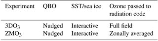
In our model experiments, we kept greenhouse gases (GHGs) and ozone-depleting substances (ODSs) fixed at 1960s concentration levels (pre-ozone hole) to get the cleanest signal possible for the ozone-wave effects. Each experiment is a freely running 100-year simulation (1955–2054) with interactive ocean and sea ice components. We run two 100-year simulations: one using the full ozone field when calculating the radiative heating rates (hereafter 3DO3 run), and one using the zonally averaged ozone field in the radiation code (hereafter ZMO3 run; see Table 1). We note that the zonal mean ozone field is used only in the radiation scheme, whereas the full 3-D ozone field is used in the ozone advection scheme. Therefore, while the ZMO3 runs exclude the radiative effect of ozone waves, they do still include the effect of ozone waves on the zonal mean ozone (and consequently on zonal mean temperature and winds) by a modification of the ozone fluxes (the second pathway described in Albers and Nathan, 2012). This formulation allows us to isolate the radiative effects of ozone waves. In the ZMO3 run, we use the full zonally varying ozone field above 1 hPa in the radiation code to avoid anomalous heating in the lower mesosphere due to the daily cycle (Gillett et al., 2009). We transition from zonally averaged ozone to a full ozone field between 2 and 1 hPa.
2.2 Diagnostics
To evaluate the different terms in the wave temperature budget, we explicitly output temperature time tendency terms from shortwave and longwave radiation, dynamics, and non-conservative processes. We use these terms to evaluate the direct ozone-wave radiative effect and compare it to other temperature time tendency terms, in particular dynamics (see the Appendix for details).
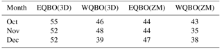
The radiative effects of ozone modulate the planetary waves and correspondingly their influence on the mean flow. These differences add up to a difference in the climatological mean. We find that the effects of ozone waves are QBO dependent. To understand the differences in planetary wave propagation depending on the phase of the QBO, and how ozone waves modulate them, we look at the life cycles of individual events of upward wave propagation from the troposphere to the stratosphere. The upward wave events are chosen based on the daily 100 hPa meridional heat flux (), averaged between 85 and 45∘ N. We chose the 100 hPa level since this is the region where the waves enter the stratosphere; however, repeating the analysis for events chosen using the 50 hPa level did not qualitatively change our results. We choose all days for which this heat flux index exceeds the 70th percentile, calculated for each calendar month from both ZMO3 and 3DO3 runs. We sort consecutive days into a single event, and events which are separated by less than 5 days are considered as single events. The central day of the event is considered as the day of the highest value. We classify the events for east/west QBOs according to the phase of the QBO. The number of events for each month and model configuration is listed in Table 2. Similar results were found for higher thresholds, but the number of events was smaller. We will mostly examine the upward wave events during the fall season, which has no negative heat flux events (no downward wave coupling). The phase of the QBO is chosen using the zonal mean zonal wind at 50–30 hPa, between 2.8∘ S and 2.8∘ N around the Equator (uQBO), where easterly and westerly QBO winters are chosen when and uQBO>5 m s−1, respectively, based on the value of winds during October each winter (choosing December made no difference). The statistical significance of the differences between two model runs (e.g., east–west QBO or 3DO3–ZMO3) is computed using a two-tailed t test, with differences exceeding the 5 % significance level marked by gray shading.
Table 2The number of positive heat flux events during east and west QBO phases (defined in Sect. 2.2), for October–December, in the 3DO3 and ZMO3 experiments.
In this section, we start with evaluating the influence of the direct radiative effect on temperature wave damping, and consequently on the wave–mean flow interaction, during autumn. We then examine the implication of these effects on the seasonal cycle of the autumn–winter season by inspecting the differences between our two simulations, with and without ozone waves passed onto the radiation code. We will see how the influence of ozone-wave effects depends on the propagation of planetary waves in the vertical and meridional directions, and how this depends on the phase of the QBO.
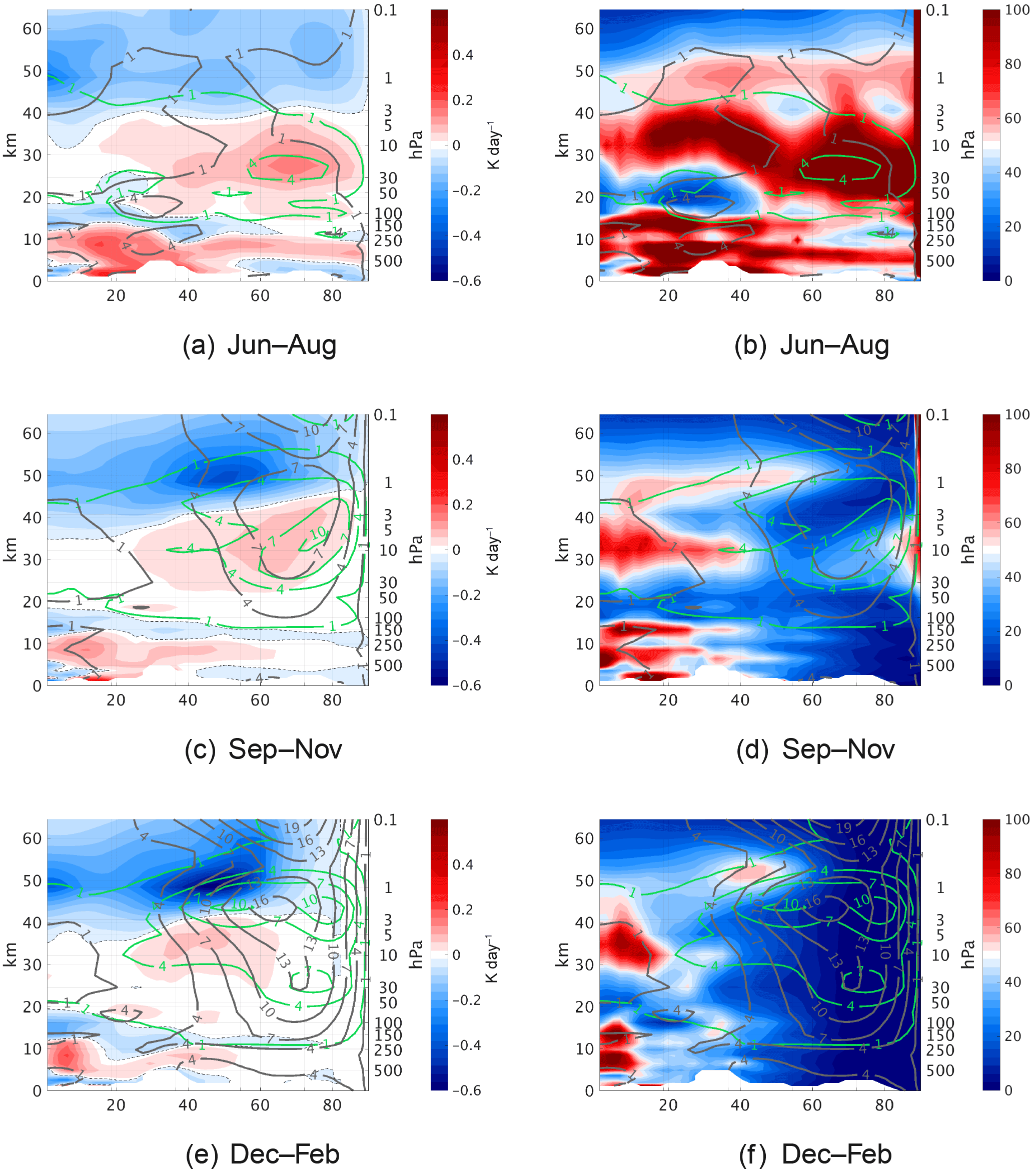
Figure 1Monthly mean temperature tendency from shortwave radiation of temperature zonal wave 1 amplitude (a, c, e), % (fraction of the tendency from shortwave radiation (SWR) of temperature zonal wave 1 amplitude compared to longwave radiation (LWR) (b, d, f), in the Northern Hemisphere during June–August (a, b), October–November (c, d), and December–February (e, f). Temperature (ozone) wave 1 amplitudes in K (10−7 kg kg−1) are shown in gray (green) contours.
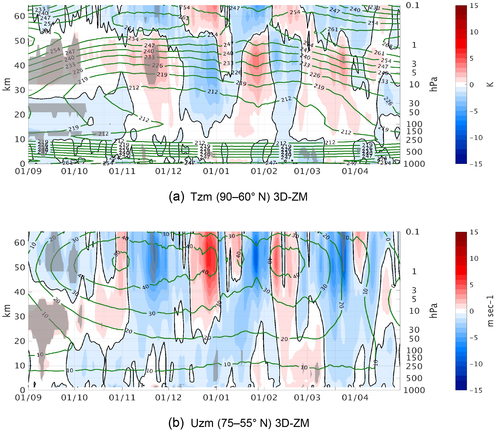
Figure 2Height–time differences between the 3DO3 and ZMO3 run for all years for zonal mean temperature, zonal wind, EP flux divergence, and temperature zonal wave 1 amplitude (from top to bottom). The differences between the 3DO3 and the ZMO3 model runs are indicated by the colored contours; the climatology of the 3DO3 run is shown by the green contours. Statistically significant areas are shown by gray shading.
3.1 The direct radiative effect
Ozone waves, via their influence on shortwave radiative heating, modulate the radiative damping of temperature waves (see the Appendix) in a way which depends on the spatial correlation between ozone and temperature waves (Craig and Ohring, 1958). In the photochemically controlled upper stratosphere (above 10 hPa), this correlation is negative, and in the transport-controlled lower stratosphere (below 10 hPa) the correlation is generally positive (Douglass et al., 1985a; Hartmann, 1981). The negative correlation in the photochemically controlled region follows naturally from the temperature dependence of ozone destruction (Craig and Ohring, 1958). The positive correlation in the dynamically controlled region is not as obvious, since it depends on the correlation between the ozone, and the meridional and vertical winds' wave perturbations, as well as on the vertical and meridional gradients of zonal mean ozone (e.g., Hartmann and Garcia, 1979). In our simulations, meridional advection of ozone is the dominant term, and correspondingly ozone wave 1 amplitudes peak where the meridional gradients of the zonal mean ozone are strongest (not shown).
The shortwave time tendencies of zonal wave 1 temperature amplitude are shown in Fig. 1, alongside the wave 1 temperature and ozone amplitudes for reference, for Northern Hemisphere summer (June–August), fall (September–November), and winter (December–February). The tendencies were calculated using Eq. (A2). The magnitude of the shortwave time tendency varies from ±0.1 to ±0.2 K day−1, while the total tendency is about ±0.5 K day−1 (not shown). It is generally positive in the lower stratosphere and negative in the upper stratosphere, with the zero line shifting from 5 hPa in the tropical region to 2–3 hPa at higher latitudes (Fig. 1a, c, e). The positive time tendency at lower levels is due to the spatial correlation of ozone and temperature being positive in this region (not shown) as a result of ozone being dynamically controlled there (Douglass et al., 1985b). The negative tendency at upper levels is due to the negative correlation between ozone and temperature due to ozone being chemically controlled at high altitudes (Douglass et al., 1985b). As predicted by previous theoretical studies, we find that ozone-wave radiative effects decrease (increase) the temperature wave damping where this correlation is positive (negative). This is also in agreement with Nathan and Cordero (2007) who found similar ozone-wave effects in a coupled ozone–chemistry Holton–Mass model. This is true for zonal waves 2–4 as well (not shown). During summer, although the wave amplitudes are small (around 1 K), the radiative effects coincide with the peak of the waves (Fig. 1b). This is also the case during fall, when the radiative effects are significant in the region where the temperature and ozone waves peak (around 7 K and kg kg−1, respectively, 80–60∘ N, 10–1 hPa). To get a sense of the importance of the shortwave effect on temperature wave amplitudes, we explicitly calculate the ratio between this term and the corresponding time tendency due to longwave radiation (the radiative damping term; Fig. 1b, d, f). We find that the shortwave time tendency reaches 40 % of the longwave time tendency (Fig. 1d). Later in winter, when the waves are stronger (around 16 K and kg kg−1, 80–50∘ N, 10–1 hPa), the radiative effects are weak at the peak of the temperature waves (around 10 %; Fig. 1f), because the radiation is weak at higher latitudes. These results are consistent with Nathan and Li (1991) who showed that ozone-wave effects are strongest during September and weakest during January due to the large solar zenith angle.
We further quantify the total wave-weighted time tendency ratio, for each calendar month separately, as follows:
where , with the subscripts tend1 and tend2 denoting two different time tendency terms, calculated from daily wave 1 temperature amplitude time tendencies, averaged over 80–50∘ N, 70–3 mb. The ratios between the different time tendency terms are shown in Table 3. We find that the relative shortwave contribution (columns 1–2) is strongest during fall (September–October) when there is enough radiation and the waves start to increase (about 19 % of the longwave cooling and 8 % of the dynamical time tendency terms during October). By November, the relative shortwave contribution decreases by 50 %, while the total radiative contribution increases compared to dynamics (third column) due to a stronger decay of the wave through longwave radiation (fourth column). We thus expect the direct ozone-wave effect to have the strongest influence during September–October. In December, the dynamics play a larger relative role, indicating the waves are becoming more non-linear. We will show in Sect. 3.4 how these radiative effects during fall modify the QBO signal at high latitudes and the mid-winter polar vortex.
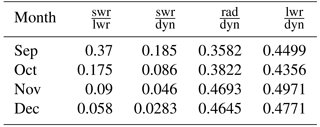
Table 3The seasonal development (October–December) of the integrated values of the following: , where , and tend1 and tend2 denote two different time tendency terms for the wave 1 temperature amplitude, averaged over 80–40∘ N, 50–0.5 mb, for the 3DO3 run. The terms shown are the time tendency terms due to shortwave and longwave radiation, and dynamics.
3.2 Radiative ozone-wave effects on the atmospheric circulation
In this section, we examine the differences in the circulation between the model run with full ozone fields passed to the radiation code (3DO3) and the run with the zonal mean ozone passed onto the radiation code (ZMO3), as described in Sect. 2.1. The shortwave radiative forcing of temperature waves in the 3DO3 model run (shown for wave 1 in Fig. 1) constitutes the primary difference in wave forcing between the two runs. Thus, we expect the 3DO3 run to have weaker temperature wave damping in the lower to middle stratosphere, and stronger wave damping in the upper stratosphere.

Figure 3September mean differences between the 3DO3 and ZMO3 run for all years for temperature wave 1 amplitude tendency from shortwave radiation (SWR) (a), temperature zonal wave 1 amplitude (b), EP flux divergence (c), and zonal wind (d). In panel (c), the gray line in the upper stratosphere indicates the height where ozone and temperature zonal wave 1 correlation changes from positive to negative. Statistically significant areas are shown by gray shading.
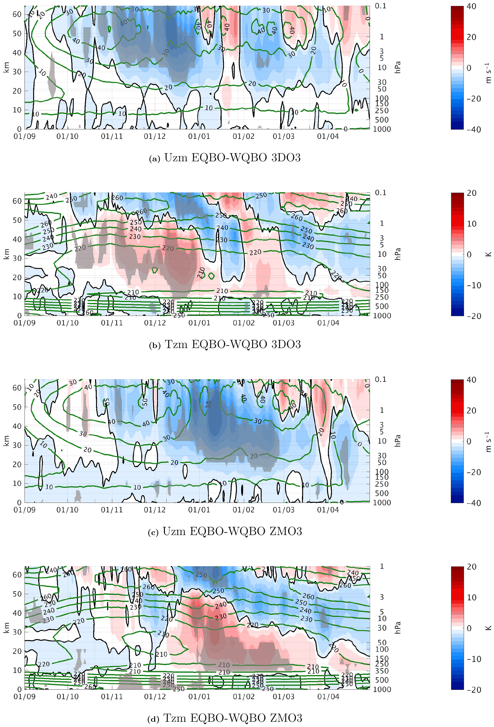
Figure 4Daily climatology differences between east and west QBO phases of the zonal mean zonal wind averaged over 75–55∘ N for the 3DO3 (a) and ZMO3 (c) runs, and the zonal mean temperature, averaged over 90–66∘ N for the 3DO3 (b) and ZMO3 (d) runs, for September–March. Statistically significant areas are shown by gray shading.
The differences in the seasonal cycle of the polar cap temperature and the polar vortex strength (the zonal mean zonal wind averaged over 75–55∘ N) between the 3DO3 and the ZMO3 runs are shown in Fig. 2 (gray shading shows regions of statistical significance at 5 % significance level). We see a significant effect during fall, when both the waves and radiation are strong enough (Sect. 3.1) and the vortex is established (green contours in Fig. 2b). The polar night jet is stronger in the lower stratosphere and weaker in the upper stratosphere in the 3DO3 run, with the upper stratospheric effect lasting until November (Fig. 2b). This is consistent with a weaker wave damping and thus stronger waves in the lower stratosphere, and stronger wave damping and thus weaker waves in the upper stratosphere (Fig. 1c). Correspondingly, the westerly jet is stronger in the lower stratosphere and weaker in the upper stratosphere as a result of an upward shift of the wave-absorption region (see next paragraph).
The above results suggest that the radiative effects of ozone waves are most robust during September–October, (Fig. 2), when the winter vortex begins to be established, solar radiation reaches high latitudes, and the waves are strong enough to be radiatively affected, while still weak enough for dynamics not to dominate completely. Under these conditions, the direct thermal damping of temperature waves by ozone waves has the largest influence. To understand how the ozone effects translate to dynamical changes, we examine the latitude–height structure of zonal wave 1 temperature and its shortwave radiative time tendency, the zonal mean zonal wind, and the EP flux convergence during September (Fig. 3). We find that the temperature wave 1 amplitude is stronger throughout the stratosphere due to the weaker damping in the lower stratosphere (Fig. 3b), resulting in an upward displacement of the EP flux convergence region where the waves decelerate the mean flow (Fig. 3c). Explicitly, there is decreased EP flux convergence in the polar stratosphere, where the wave damping is reduced (note the gray line marking where the shortwave radiative damping changes sign), and increased EP flux convergence in the upper stratosphere/lower mesosphere where the wave damping is stronger. The EP flux convergence also increases at lower latitudes, where more wave activity reaches due to the reduced high-latitude convergence (Fig. 3a). This causes the polar night jet to strengthen in the lower stratosphere and weaken in the upper stratosphere (with a poleward tilt; Fig. 3d), with the upper stratospheric deceleration lasting until November (Fig. 3d). The above robust direct radiative effect disappears after November (Fig. 2), most likely as a result of the seasonal reduction in shortwave radiation and the strengthening of the dynamical processes. Nathan and Li (1991) found that when the waves peak in the region where ozone and temperature are positively correlated, the main ozone-wave effect is to strengthen the waves due to the weaker radiative damping, whereas when the waves peak higher in the region of negative ozone–temperature correlation, the dominant ozone-wave effect is the increased radiative damping. In our model, we see the dominant effect is to increase wave amplitudes throughout the midlatitude stratosphere. Apart from the obvious model differences (1-D vs. CCM), it is possible this is also due to the fact that, in the ZMO3 run, we zonally average the ozone field only in the stratosphere, in order to avoid large biases from tides in the mesosphere.
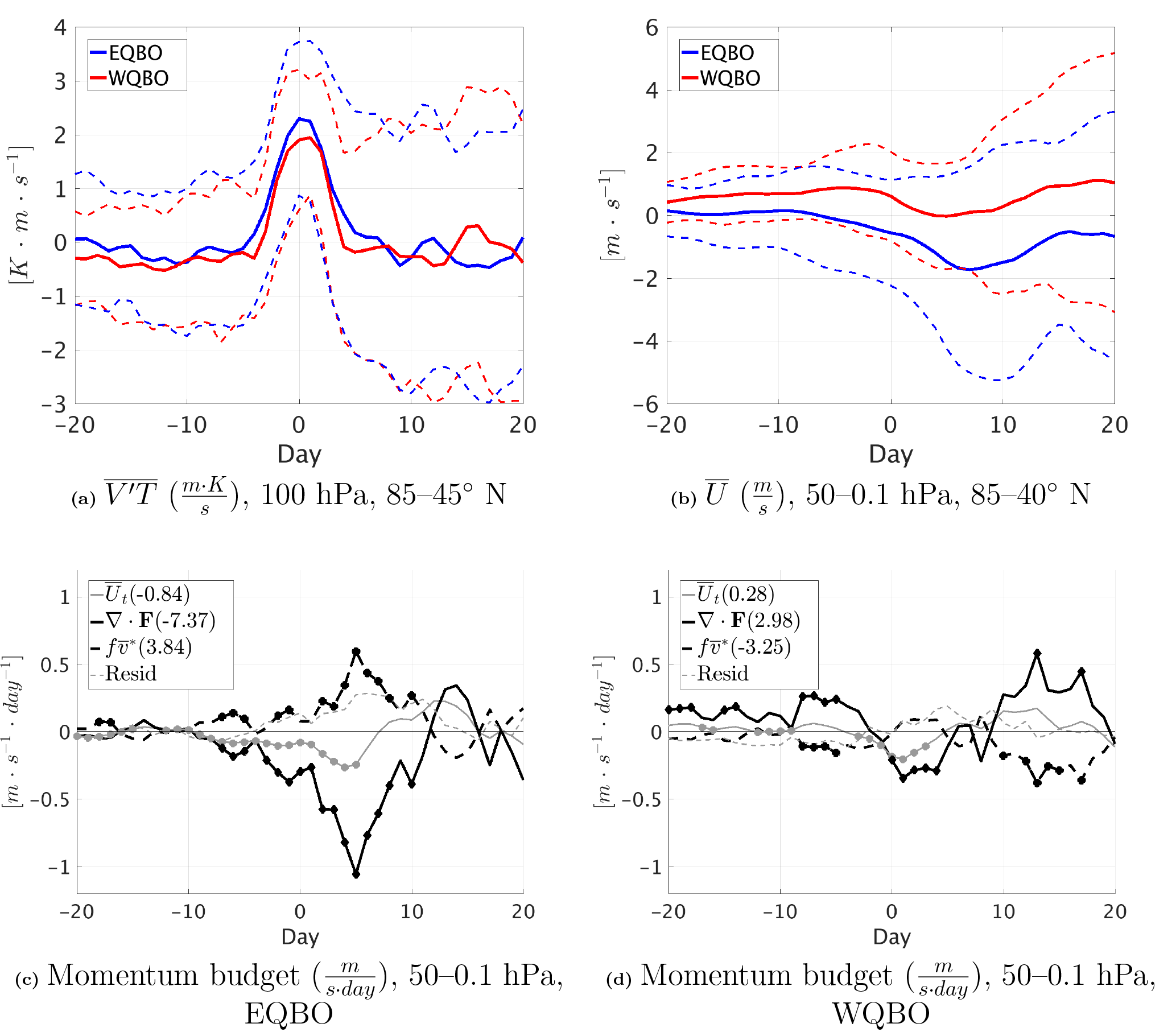
Figure 5Time lag composites for the upward wave pulse events during October in the 3DO3 run. (a) averaged over 85–45∘ N at 100 mb. (b)–(d) The extratropical stratospheric averages (50–0.1 mb, 85–40∘ N, marked by the green rectangle in Fig. 6a of (b); dashed lines show ±1 standard deviation. (c)–(d) Momentum budget terms for east and west QBO events, respectively. Shown are the total time tendency (thin gray), (dashed black), and the residual (gray dashed) with their integrated value from days −10 to 20 denoted in the figure legend.
The results shown in Fig. 2 appear to suggest that the winter midlatitude stratosphere is not sensitive to the inclusion of radiative ozone-wave effects. While there is a significant radiative effect during fall, it seems to disappear later on. In the next section, we will show, however, that this lack of a response is due to the response being oppositely signed between east and west QBO phases, so that there is a cancellation when all years are considered.

Figure 6Time lag composite of the zonal mean zonal wind anomalies for east QBO (a), west QBO (b), and the difference between them (c) for the positive heat flux events from the 3DO3 run of October. The green box in row (a) shows the area of averaging for Fig. 5b–d.
3.3 The onset of the midlatitude QBO signal in fall and its modulation by ozone waves
The influence of the tropical QBO phenomenon on the extratropical region, known as the Holton–Tan effect, consists of a weaker and warmer polar night vortex during the easterly phase of the QBO. Figure 4 shows the east–west QBO seasonally varying polar vortex strength and polar cap temperatures, alongside the climatological seasonal cycle based on all years, for the 3DO3 and ZMO3 runs. In the 3DO3 run, the Holton–Tan effect starts in October, with a weaker vortex (Fig. 4a) and a warmer polar cap (Fig.4b) during the easterly QBO phase. In the ZMO3 run (Fig. 4c–d), the Holton–Tan effect is delayed, with the robust signal starting about 2 months later, in January instead of November. The calculation of the statistical significance for the difference between Fig. 4a and d is described in Appendix A1.
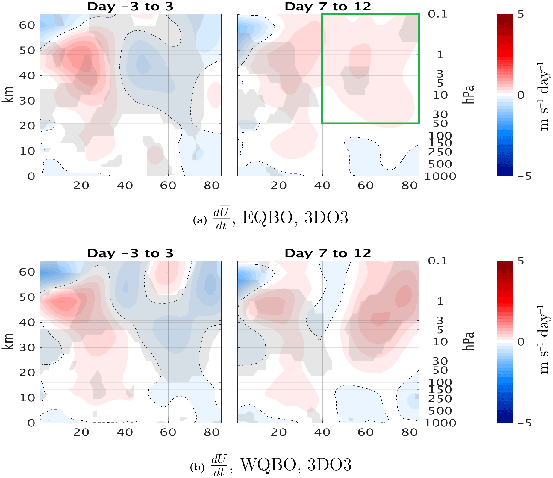
In order to understand the different seasonal development of the midlatitude QBO signal between 3DO3 and ZMO3 runs, we examine the life cycles of upward-propagating wave pulses entering the stratosphere during October, when the midlatitude QBO effect starts, and compare them between the two QBO phases. We take the strongest 30 % of 100 hPa 85–45∘ N mean heat flux events1 and divide them according to the phase of the QBO. Figure 5 shows heat flux pulses (Fig. 5a), which induce a deceleration of the jet a few days after the peak 100 hPa heat flux pulse (Fig. 5b), followed by an acceleration which partly reverses it. We see that while the heat flux pulses are quite similar in magnitude and length, the wave-induced deceleration is stronger, and the subsequent acceleration is weaker, during east QBO. More specifically, during east QBO the winds do not accelerate back to the values before the wave pulse, while during west QBO the acceleration completely reverses the deceleration, leaving the vortex with similar strength. Since the anomalies are based on a climatology of the full run, we see part of the east–west QBO difference already at negative time lags, but this difference grows with each upward wave pulse. This is more clearly illustrated in latitude–height composites of the zonal mean zonal wind at different stages of the wave life cycle for east and west QBO phases (Fig. 6). The tropical QBO signal is evident, as well as a small but significant midlatitude QBO signal of opposite signs. This midlatitude signal is evident between 40 and 60∘ N at all stages, even at negative time lags. During the peak of the event (days −3 to 3), we see a weakening of the zonal wind anomalies at high latitudes and all levels, but this weakening is much clearer during east QBO. At later stages, on the other hand, the winds strengthen back, essentially spreading the initial anomaly between 60 and 40∘ N to polar latitudes. The strengthening of the midlatitude QBO signal over the life cycle is seen clearly when looking at the differences between the east and west composites (Fig. 7c). To isolate the effect of the wave pulse from the preexisting QBO signal, we composite the zonal mean zonal wind time tendency (Fig. 7). We see a clear deceleration of the vortex during the peak of the event (days 3 to −3) for both QBO phases, with a slightly stronger deceleration during east QBO. The largest difference is during the end of the life cycle (days 7 to 12); while there is a very weak acceleration during east QBO, the acceleration is comparable in magnitude to the deceleration during west QBO.
To better understand the polar vortex evolution, we composite the zonal momentum budget (see Andrews et al., 1987, Eq. 3.5.2a) (Fig. 5c–d). During east QBO events, the deceleration is driven by a clear EP flux convergence which is counteracted by the Coriolis term, while during west QBO, these terms are much weaker. This is quantified more clearly by time integrating the different time tendency terms over the life cycle (days −10 to 20; values indicated in the figure legend). In particular, the time-integrated represents the reversibility of the wave life cycle. In particular, the positive value for the west QBO events (Fig. 5d) indicates the wave-induced deceleration is more reversible, while the negative value of the east QBO events (Fig. 5c) shows that a significant part of the wave-induced deceleration of the mean flow remains after the life cycle has ended.
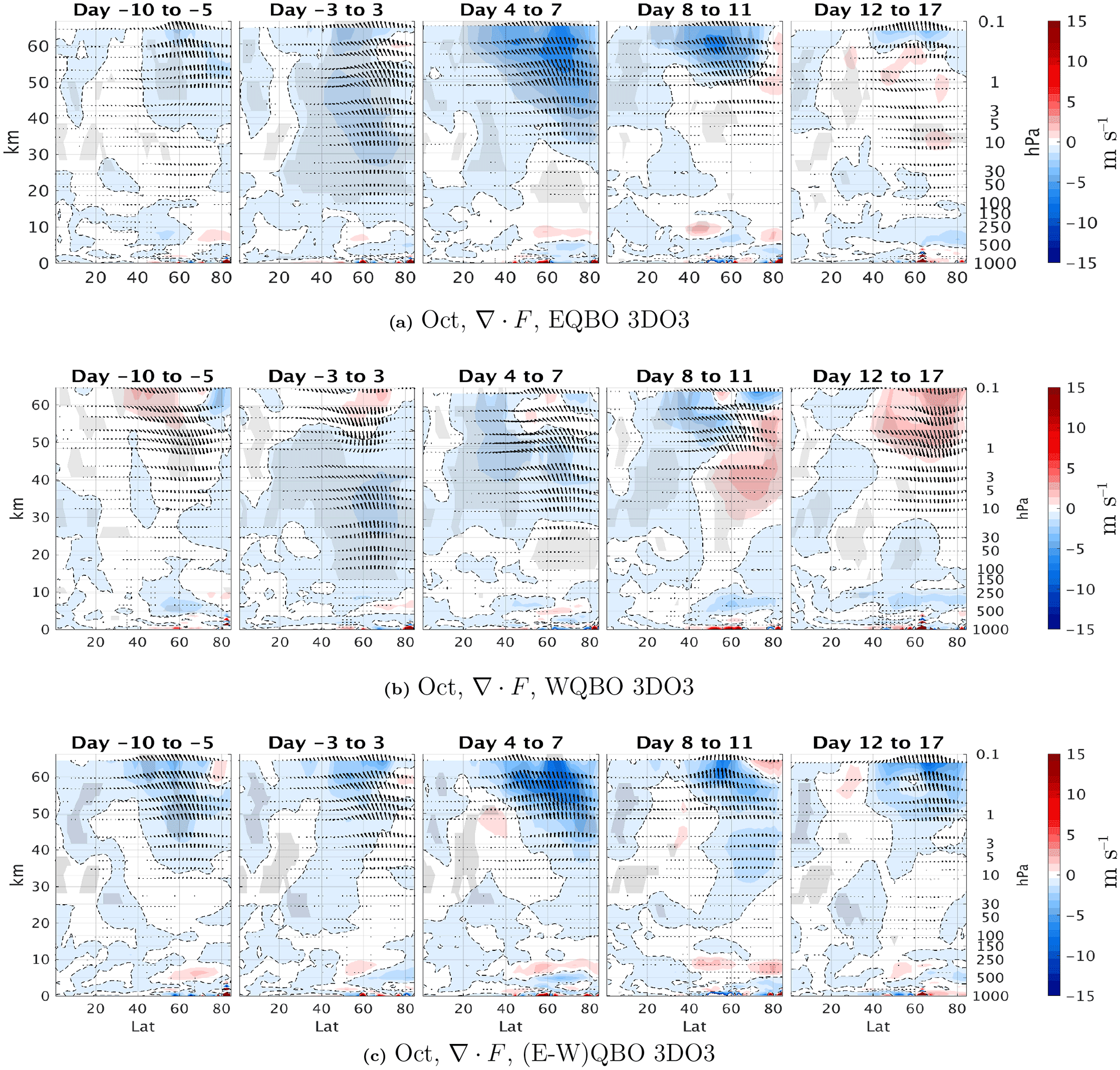
Figure 8Latitude–height time lag composites of EP flux divergence (anomalies from the climatology) for the positive heat flux events (70th percentile of at 100 mb, 85–45∘ N) for east (a), west (b), and the their differences (c) for October events for the 3DO3 run. Statistically significant areas are shown by gray shading.
To understand why the life cycle of west QBO events is more reversible, we look at the latitude–height daily time lag composites of EP flux divergence anomalies (Fig. 8). There is stronger convergence (more negative values) at the high-latitude upper stratosphere during east QBO events at days −3 to 7 (Fig. 8a, c), while during west QBO events, there is increased convergence in the subtropical region (Fig. 8b, c). This suggests the waves propagate up along the polar vortex and break in the upper polar stratosphere during east QBO, while they refract equatorwards in the middle stratosphere during west QBO. This difference in wave propagation can be explained when examining the index of refraction just prior to the upward wave pulse events (days −5 to −10; Fig. 9). The index of refraction is stronger in the high-latitude upper stratosphere during east QBO and stronger in the midlatitude subtropics during west QBO. A separation into vertical and meridional wavenumbers (see Harnik and Lindzen, 2001) suggests the main contribution to these changes comes from the vertical wavenumber. This is consistent with the waves propagating to the upper polar stratosphere during east QBO and more equatorwards during west QBO. At later stages of the wave life cycle (days 8–17), during west QBO, there is a significant anomalous EP flux divergence, indicative of anomalous acceleration. This is consistent with a wave packet trailing-edge acceleration, expected to occur under non-acceleration conditions of linear inviscid waves (Andrews et al., 1987). During east QBO, we see no such EP flux divergence region. This suggests the following picture: during fall, after the westerly winds get established and planetary waves start propagating up to the stratosphere, the waves are weak enough to be linear in the lower–middle stratosphere. Under these conditions, only waves which propagate up the polar vortex to the upper stratosphere/mesosphere grow enough (due to the density effect) to break non-linearly. This happens during east QBO, and the deceleration induced by the breaking waves is irreversible in large part. During west QBO, the waves refract to the Equator before reaching levels where they become significantly non-linear; thus, they decelerate the vortex when propagating up and accelerate it when refracting equatorwards. The strong acceleration is enabled due to non-acceleration conditions being satisfied. 2
To explicitly examine the degree to which non-acceleration conditions are satisfied, we inspect the enstrophy budget and see how the different terms balance during these heat flux events. Following Eq. (3) from Smith (1983), for the enstrophy balance, we get
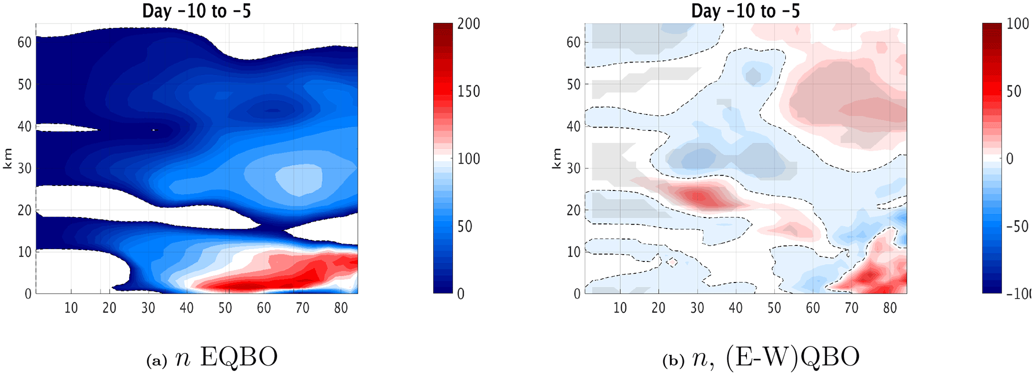
Figure 9Index of refraction ; see Eq. (C2,5) in Harnik and Lindzen (2001) at days −10 to −5 for (a) east QBO and (b) the difference between east and west QBOs in the 3DO3 run.
Primes denote the deviation from the zonal mean, q is the quasi-geostrophic potential vorticity (QGPV), and D′ is the temperature time tendency from diabatic heating:
where Q′ is the temperature time tendency from radiation, both short- and longwave. On the right-hand side of Eq. (1), the first term is the wave–mean flow interaction, equivalent to the EP flux divergence multiplied by the meridional gradient of the zonal mean potential vorticity (), the second and third terms are the non-linear terms, the fourth and fifth terms are the diabatic terms from shortwave and longwave radiation, and the last term is the residual of the total time tendency minus all the terms on the right-hand side. Large non-linear, damping, and residual terms indicate a violation of non-acceleration conditions (Andrews et al., 1987).
Figure 10 shows the time-lagged composites of the different enstrophy budget terms of Eq. (1), averaged over 70–40∘ N, 50–1 hPa. The averaging area was chosen based on an examination of latitude–height composites. We see that during both QBO phases, the enstrophy time tendency (blue lines in Fig. 10) is driven by the linear term (black lines in Fig. 10) and slightly damped by thermal damping (magenta lines in Fig. 10), but the non-linear (red lines in Fig. 10) and residual terms (gray lines in Fig. 10) are large and significant during east QBO, and are much smaller during west QBO. This is consistent with White et al. (2016) who used reanalysis data to study the different seasonal cycles between east and west QBOs, and found that non-linear interactions are stronger during November–January of east QBO years. These results suggest that the dynamics during west QBO are more reversible (closer to non-acceleration). We note, however, that during east QBO, the non-linear terms act to reduce wave enstrophy, while the residual acts to increase it. The cancellation is quite large, and in fact, the sum of the non-linear and residual terms gives a slightly negative value which is only slightly more negative during east QBO. The residual terms, however, are very noisy, while the non-linear terms have a coherent spatial structure, so that this cancellation only occurs when we take a latitude–height average. The large residual may be an artifact of our having daily, rather than shorter, timescale output, and further examination is needed to better understand the role of non-linearities.
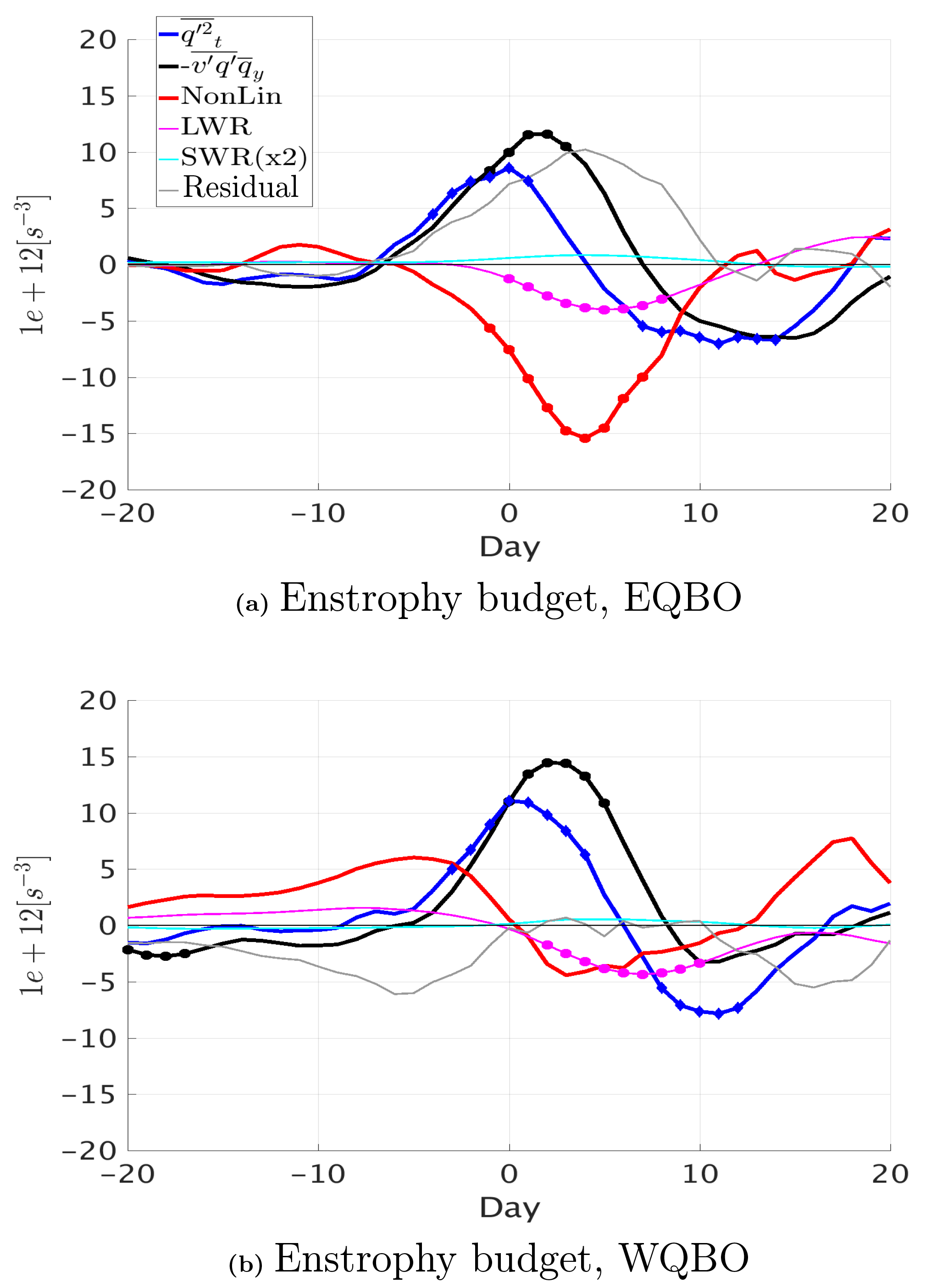
Figure 10Time lag composite of the enstrophy budget terms (1×10¹² s−3) for east (a) and west (b) QBOs, averaged over 70–40∘ N, 50–0.1 mb, for the positive heat flux events from the 3DO3 run of October.
We now turn to examining the role of ozone waves by repeating the analysis for the ZMO3 run. Figure 11 shows the time-lagged composites of the EP flux and its divergence (compare to Fig. 8). The main point to note is the lack of strong anomalous EP flux convergence at positive time lags during west QBO, which for the 3DO3 run made the west QBO wave-induced deceleration reversible. This weaker trailing-edge acceleration for the ZMO3 run is consistent with a stronger radiative damping of the waves in the lower–middle stratosphere as a result of removing the tendency of ozone waves to weaken the radiative damping in these regions (Fig. 1c). In addition, during east QBO, there is weaker EP flux divergence in the upper stratosphere on days 4 to 7, consistent with a weaker wave damping as a result of removing the tendency of ozone waves to increase radiative damping there (Fig. 1c).

Figure 11Latitude–height time lag composites of EP flux divergence anomalies from the climatology for the positive heat flux EQBO (a), WQBO (b), and the difference between them (c) for October events (70th percentile of at 100 mb, 85–45∘ N) of the ZMO3 run. Statistically significant areas are shown by gray shading.
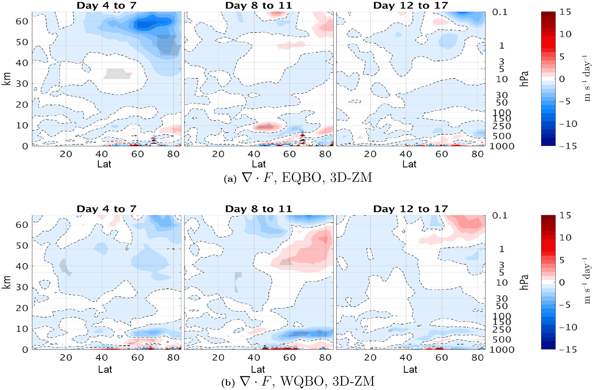
Figure 12Latitude–height time lag composites differences of the 3DO3 and ZMO3 runs of the EP flux divergence (colors) for east QBO years (a) and west QBO years (b) for October events (70th percentile of at 100 mb, 85–45∘ N). Dashed contours indicate negative values. Statistically significant areas are shown by gray shading.
The above results suggest that ozone waves affect the total wave-life-cycle mean EP flux divergence in an opposite sense between east and west QBO phases – they decrease it during west QBO and increase it during east QBO. A closer examination shows that this is due to the differences in wave propagation and damping patterns, which causes the ozone-wave damping to affect the EP flux divergence during different times of the wave life cycle during the two QBO phases (Fig. 12). During east QBO, the EP flux divergence is stronger in the upper stratosphere during the peak of the deceleration (days 4–7) in the 3DO3 run, consistent with the waves being damped more strongly in the upper stratosphere. During west QBO, there is a significant EP flux anomalous convergence in the upper stratosphere at late stages of the life cycle in the 3DO3 run, which is absent in the ZMO3 run, consistent with a weaker ozone-induced damping strengthening the trailing edge effect.
Besides a difference due to changes in wave propagation pattern, it is also possible that the shortwave thermal forcing itself varies between east and west QBOs due to changes in the amplitude of ozone waves and the correlations between ozone and temperature anomalies. An examination of the wave 1 ozone budget shows weaker ozone waves during east QBO due to weaker meridional gradients of zonal mean ozone during east QBO. This weakening of the ozone waves is accompanied by a reduction of the shortwave damping in the lower to middle stratosphere and a strengthening of the total radiative wave damping. The temperature wave amplitude, however, is still stronger during east QBO, suggesting the effects of changes in zonal mean ozone gradients are of second order.
3.4 The subsequent seasonal evolution of ozone-wave effects
As seen in Sect. 3.1, the direct radiative ozone-wave effect starts very early on in September, when the waves just emerge from the troposphere and are not yet affected by the phase of the QBO. The main effect is to increase the EP flux convergence in the upper stratosphere (Fig. 3c) and slightly weaken the vortex (Fig. 3c). During October, when the waves grow a bit, we see that individual wave life cycles are significantly affected by the phase of the QBO, so that the wave-induced deceleration is slightly stronger during east QBO compared to west QBO. The ozone-wave radiative interaction affects individual life cycles in an opposing manner between east and west QBO phases, which strengthens the east–west QBO differences. This was shown explicitly only for October life cycles, but we find similar life cycle behavior during November as well. As a result, the stronger EP flux convergence during east QBO strengthens and descends lower down as the winter evolves (not shown), resulting in a weaker polar vortex by November during east QBO years (Fig. 13a, green line).

Figure 13Daily climatology of EQBO (a) and WQBO (b) years (defined by October) averaged over 10–0.1 mb, 85–45∘ N. The EP flux divergence is shown for the 3DO3 run (black), the ZMO3 run (blue), and their difference (red), with the difference between 3-D and ZM runs of the zonal mean zonal wind shown in green. Gray and blue shading indicated ±1 standard deviation from the mean of the 3DO3 and ZMO3 runs, respectively. Statistical significance is indicated by a thick line.
Later in the winter, the waves become stronger and more non-linear, and shortwave radiation decreases. As a result, the direct effect of ozone waves is strongly reduced and a modulation of wave–mean flow interaction takes over the midlatitude QBO signal in the form of a polar night jet oscillation (Kuroda and Kodera, 2001), which arises because changes in the vortex strength affect the strength of the waves and their induced deceleration, while changes in the waves affect their deceleration of the vortex. This is evident from Fig. 13, which shows the daily climatology and the interannual range of the EP flux divergence, integrated over 85–45∘ N and 10–0.1 hPa, for the 3DO3 (black) and ZMO3 (blue) runs and their difference (red). Also shown is the difference in the vortex-integrated zonal mean wind for 3DO3–ZMO3 runs (green) for east (Fig. 13a) and west (Fig. 13b) QBO years. We see the ozone-wave influence described in the previous two sections – a very small but significant weakening of the vortex for 3DO3 compared to ZMO3 for both QBO phases during September, which strengthens in October for the east QBO but reverses sign in October of west QBO. This preconditioning of the winter vortex initiates an oscillation between the anomalies of EP flux divergence and zonal mean zonal wind, similar to that which gives rise to the “polar night jet oscillation” (Kuroda and Kodera, 2001): less wave-induced deceleration leads to a weaker jet, which in turn reduces the amount of waves propagating up the vortex, allowing the vortex to strengthen from mid-December. We note, however, that although the anomalies in EP flux divergence and zonal mean winds are much larger during mid-winter compared to fall, they are not statistically significant over most of the winter (Fig. 13a, red and green lines). This is due to the large interannual variability (wide gray shading region) and the occurrence of occasional sudden stratospheric warmings. During west QBO, these cycles start in the opposite phase compared to east QBO, with stronger EP flux divergence, followed by a stronger vortex, which is followed by more waves propagating up the vortex, and subsequent deceleration (Fig. 13b, red and green lines). These induced changes in the circulation cause a dynamical cooling (heating) during December (January) in the lower stratosphere, and heating (cooling) during December (January) in the upper stratosphere/lower mesosphere (not shown). We note that only the latter part of the cycle is statistically significant, suggesting the radiative effects of ozone waves are less robust during the west, compared to the east, QBO, with the most robust signal showing up in their difference.
We also find statistically significant 3DO3–ZMO3 anomalies of zonal mean ozone concentration of about 6–8 % in the polar mid-stratosphere, starting from September (not shown). Consistently, the zonal mean shortwave radiation heating anomalies reach up to 10 % of the climatological time tendency in early winter (0.05 K day−1 in September–October), though they are much weaker later in mid-winter (not shown). These changes are much weaker in the west QBO phase (about half the magnitude) during October and are not statistically significant during November. These changes may provide feedback on the ozone-wave radiative effects through modulation of the ozone-wave amplitudes and might be an additional cause to the east–west QBO differences in the winter march. This is different from Albers et al. (2013), who noted that zonal mean ozone variations were negligible.
In this study, we examined the radiative effects of ozone waves on the midlatitude polar vortex using a set of CESM-WACCM model runs in which a control simulation with a nudged QBO is compared to a run where only the zonal mean part of the ozone field is passed on to the radiative heating code. We find a weak but significant effect during September, when the westerly polar vortex just starts getting established, which is not dependent on the phase of the QBO (Fig. 3).
Later on, in October, ozone-wave heating affects the life cycles of upward-propagating waves, and since the wave life cycle is different for east and west QBOs, the ozone-wave effect is also different and opposite. As a result, it is only significant when considering each QBO phase separately (Fig. 4). Moreover, in the 3DO3 run, the midlatitude effect of the QBO starts earlier in the season, in October, compared to December in the ZMO3 run (Fig. 4). This shortwave radiative influence of the waves only occurs during fall when the waves are still weak (compared to mid-winter) and radiation is still strong, yet the individual wave-life-cycle effects accumulate to a significant preconditioning which influences the subsequent development of the mid-winter polar jet.
It is interesting to compare our results to previous studies. We find that ozone waves weaken the zonal mean winds most robustly during fall (with a peak in November; Fig. 2). These results are consistent with Gillett et al. (2009) who found an ozone-wave-induced weakening during October to December. McCormack et al. (2009), on the other hand, found a response in January–February; however, they ran a pair (an ensemble of pairs) of December–March simulations with similar initial conditions, while Gillett et al. (2009) used a 40-year simulation of the entire seasonal cycle, with a spontaneously produced realistic QBO in their model (Scinocca et al., 2008). This suggests that the inclusion of a full seasonal cycle allows the ozone-wave influence to appear in fall and to be less significant later in the winter when internal variability takes over. Moreover, the existence of a realistic QBO in our runs masks the signal in mid-winter if the analysis is done averaging both QBO phases together – it will be interesting to see how the analysis of Gillett et al. (2009) would change if the results are stratified by the phase of the QBO. Starting the simulation in mid-winter (December), with similar initial conditions for the 3DO3 and ZMO3 runs (as in McCormack et al., 2009), helps get a cleaner ozone-wave signal in late winter, despite the weaker shortwave radiation and stronger waves. It is also interesting to compare our results to the more simplified 1-D model Nathan and Cordero (2007) used for mid-winter conditions. Their results are most comparable to our results during fall (September) – they found decreased EP flux convergence in the lower stratosphere where ozone waves reduce the radiative damping on temperature waves (they find a reduction of ∼ 25 %, while we find ∼ 10 %), and an increase in EP flux convergence is 2 times stronger in the upper stratosphere where ozone waves increase the radiative damping (while we find ∼ 10 %).
The dependence of the radiative ozone-wave effects on the phase of the QBO during early winter was examined by compositing individual wave life cycles during October for east and west QBOs separately. We find that the life cycle during west QBO is more reversible (Fig. 5d), allowing the polar night jet to recover from the deceleration which an upward-propagating wave pulse induces (Fig. 5b). The small differences of single wave events add up, and the cumulative effect is consistent with the known Holton–Tan effect resulting in a stronger polar vortex during west QBO years. We further showed that this difference occurs a month earlier in the 3DO3 run (Fig. 4). In the east QBO events, there is stronger EP flux convergence at the upper levels (Fig. 8a), which is further increased in the 3DO3 run in early winter. As winter progresses, the deceleration is extended poleward and downward. During west QBO, ozone waves weaken the wave damping in the lower stratosphere and render the dynamics more reversible. In particular, the acceleration at the trailing edge of the waves, which is responsible for this reversibility, is stronger in the 3DO3 run, resulting in an earlier Holton–Tan signal. This synoptic-type life cycle analysis, done separately for the different QBO phases, provides an additional mechanism to understand the Holton–Tan effect. For example, Watson and Gray (2014) did not find a fall–early winter Holton–Tan effect (as is found in the observations). While they suggest their delayed response has to do with the response timescale to tropical wind anomalies, it is also possible that their use of zonal mean ozone in the radiative code of their model also contributes to this delay. It is not clear, however, if the strengthening of the Holton–Tan effect by ozone waves is unique to our model, or if it holds for other models as well. It is also possible that a lack of ozone-wave effects may explain the weak Holton–Tan effect produced by climate forecast models (Smith et al., 2016) and might improve the predictability if included (Scaife et al., 2014). Our results may also help understand the influence of the 11-year solar cycle on the polar vortex and its dependence on the QBO phase (e.g., Labitzke and Van Loon, 1988; Garfinkel et al., 2015). For example, it is possible that the solar cycle modulates the strength of the ozone-wave radiative forcing.
Finally, our model setup used fixed GHGs and ODSs at 1960s levels. Under this configuration, ozone waves are weaker compared to the 1990s (not shown); thus, we expect the ozone-wave effects to be stronger in runs with present-day forcings, and it remains to be examined how these effects might change in the future.
The CESM(WACCM) model data requests should be addressed to Katja Matthes (kmatthes@geomar.de).
A1 Statistical significance of Fig. 4
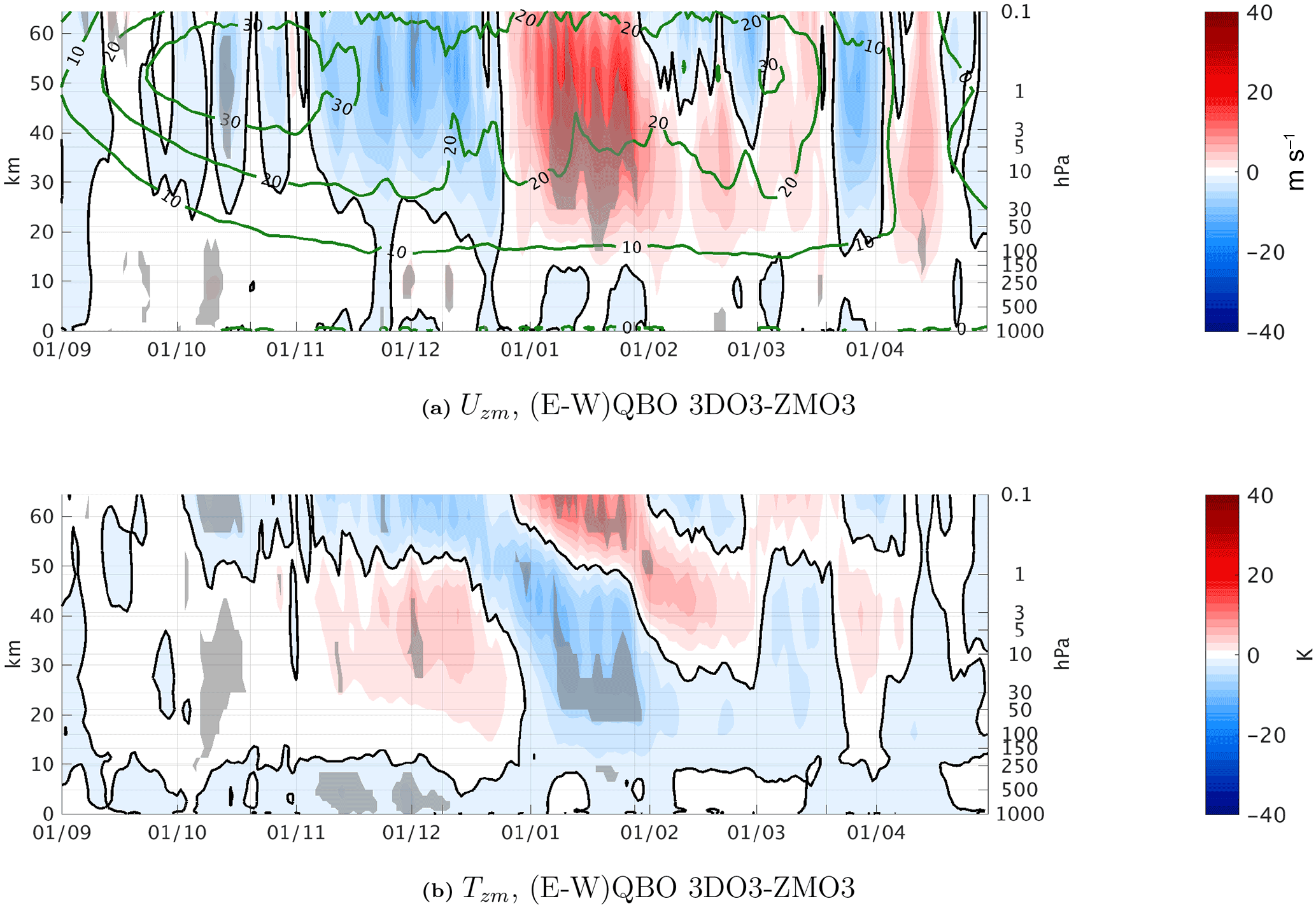
Figure A1Daily climatology east–west QBO differences between the 3DO3 and ZMO3 model runs of the zonal mean zonal wind averaged over 75–55∘ N (a) and the zonal mean temperature averaged over 90–66∘ N for the 3DO3 (b) for September–March. Statistically significant areas are shown by gray shading.
To calculate the statistical significance of the difference between these two figures, we need to have any realizations of each model run. Since this is not possible, we do the following:
-
We take all years of the two simulations – a total of 200 years.
-
We randomly choose a set for two groups of years according to the number of east/west QBO years in each run (two groups for 3DO3 and two for the ZMO3 run).
-
We then average each group and take the difference between then as an east–west mean for each simulation.
-
We repeat this 1000 times.
We now have 1000 differences of random years for each run. Statistical significance of the 3-D(E–W) and ZM(E–W) is calculated similarly but checking if the difference of the E–W (3-D–ZM) is bigger/smaller than the 97.5/2.5 percentile of the difference between the two distributions we got.
The result of this calculation is shown in Fig. A1 for the zonal mean zonal wind (top) and zonal mean temperature (bottom). In the zonal mean zonal winds, the negative/positive values in early/late winter indicate that the E–W difference in the 3DO3 run is stronger/weaker than the E–W difference in the ZMO3 run, corresponding to a delay in the Holton–Tan (HT) signal. The differences are statistically significant. The delayed HT signal in the zonal mean temperature is statistically significant as well.
A2 Estimating the direct ozone effect (wave 1 amplitude tendencies)
We focus on zonal wave number 1 since it is the most dominant in the stratosphere. The main balance of temperature time tendency is given by
For the zonal wavenumber 1 amplitude balance, we use the equations above, apply Fourier transform, and take the first wave component. After that, we have the following complex terms for temperature wave balance (s1 denoting first Fourier component):
To estimate the time tendency of the temperature wave amplitude from each term in each time step, we use the following procedure:
-
Calculate the complex of the next time step from each term: , where “term” is either advection (total or one component), residual, or each of the tendencies from the model/reanalysis.
-
Calculate the change in amplitude: , where is the amplitude tendency from a specific term.
It is important to note that this calculation implies the amplitude tendencies from each term do not add up to the total time tendency; however, it represents best how each process “attempts” to the change the wave amplitude.
A3 Radiative ozone-wave effects on the atmospheric circulation during summer
In Sect. 3.1–3.2, we showed the direct radiative effect of ozone waves on the circulation during September. Here, we examine the differences between 3DO3 and ZMO3 runs during summer to verify that the September anomalies are not simply carried over from summer. In particular, an examination of the 3DO3–ZMO3 zonal mean shortwave heating during summer (Fig. A2c) reveals a thin band of stronger heating in the 3DO3 run, right at the levels where the model changes back to using 3-D ozone in the radiation code in the upper stratosphere which persists into fall. Though this region is significantly reduced to a very small latitude range in early winter (less than 5∘ in the subtropical region), we need to verify that it is not the source of differences between the 3DO3 and ZMO3 fields during fall and winter.
We find a few indications that this is not the case. First, looking at the zonal mean temperature and the contribution of dynamics to the temperature time tendency, we find small but significant differences in the zonal mean temperature (Fig. A2a). The polar stratosphere is warmer above 20 hPa and colder below in the 3DO3 run during May–August by about 1 K. Similar differences are found in Gillett et al. (2009) (Fig. 3d). These differences are dynamically driven as indicated by the zonal mean temperature time tendency from dynamics (Fig. A2b). It is possible, however, that the source of differences in the dynamical time tendencies is this anomalous band of shortwave heating. Fig. A3 shows the 3DO3–ZMO3 differences of different terms in the zonal mean zonal wind time tendency equation. The zonal mean zonal wind of the 3DO3 run is more westerly in the subtropical lower stratosphere in July, extending upward and poleward until August (Fig. A3a). There is a vertical displacement of the EP flux convergence height, with decreased convergence in the lower stratosphere and increased convergence above 30 mb (Fig. A3b), well below the region of negative ozone–temperature correlation (indicated by the gray line in the figures). This demonstrates that the vertical displacement of the convergence region is due to the waves reaching higher due to their stronger amplitudes. The total time tendency and the related zonal mean zonal wind anomalies are governed by these changes only during August–September. Earlier in summer, the time tendency is controlled by the tendency from the Coriolis torque term () above 30 mb (Fig. A3c) and by the EP flux convergence below.
Finally, in addition to the runs described in this paper, we conducted four 40-year time slice experiments, for which we specified constant east or west QBO phases, for 3DO3 and ZMO3. While the summer heating bands also appeared during summer in these runs, the differences in the Holton–Tan effect between 3DO3 and ZMO3 runs during fall and winter were not found. An examination of October upward wave pulses showed that in both runs there is a stronger EP flux divergence during the late stages of the wave life cycles in the west compared to the east QBO phases, but this acceleration is due to non-linear wave–mean flow interactions rather than to a linear trailing edge acceleration. Correspondingly, the waves are stronger at 100 mb in the time slice experiments during October (we are still examining the reasons for these differences). Nonetheless, this suggests that summer heating band is not the source of differences between the 3DO3 and ZMO3 runs found in fall and winter in our time-varying QBO 100-year experiments.
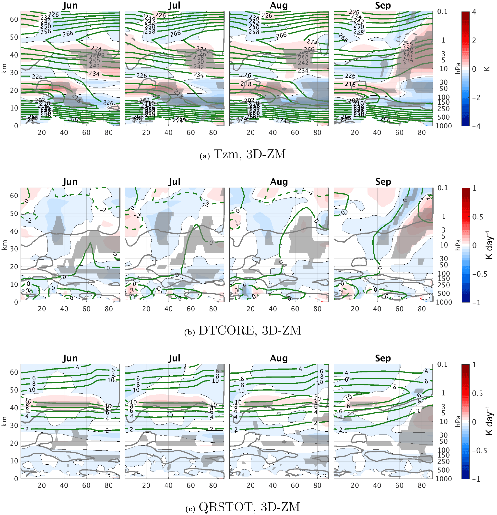
Figure A2Monthly climatology differences between 3-D and ZM ozone runs during summer, June–September of the zonal mean temperature (a), zonal mean temperature tendency from dynamics (b), and shortwave radiation (c). Statistically significant areas are shown by gray shading.
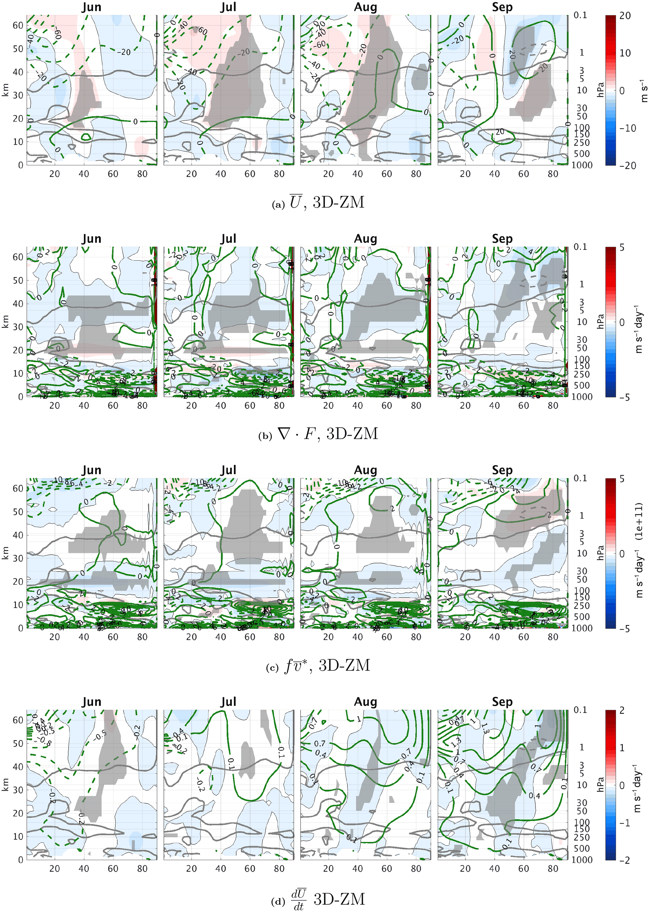
Figure A3Monthly climatology differences between 3-D and ZM ozone runs during summer, June–September of the zonal mean zonal wind (a), zonal mean zonal wind tendency from EP flux convergence (b), the time tendency from the Coriolis term (c), and the total time tendency (d). Statistically significant areas are shown by gray shading.
The authors declare that they have no conflict of interest.
We wish to thank the anonymous reviewers for their useful comments. We also wish to thank Chaim Garfinkel for our fruitful discussions.
This work is supported by the German-Israeli Foundation for Scientific Research and Development, under grant GIF1151-83.8/2011, and by the Israel Science Foundation (grants 1537/12 and 1685/17). This work has also been partially performed within the Helmholtz University Young Investigators Group NATHAN funded by the Helmholtz Association through the Presidents Initiative and Networking Fund and the GEOMAR – Helmholtz Centre for Ocean Research Kiel, Germany. The model simulations were performed at the German Climate Computing Centre (Deutsches Klimarechenzentrum, DKRZ) in Hamburg, Germany.
Part of the work of Nili Harnik was done while on sabbatical at Stockholm University, and supported by a Rossby Visiting Fellowship from the International Meteorological Institute of Stockholm.
We also acknowledge GOAT (Geophysical Observation Analysis Tool; http://www.goat-geo.org) for the data storage organization.
We acknowledge the Israeli Atmospheric and Climatic Data Center, supported by
the Israeli Ministry of Science, Technology and Space, for assisting with the
data handling.
Edited by: William
Ward
Reviewed by: two anonymous referees
Albers, J. R. and Nathan, T. R.: Pathways for communicating the effects of stratospheric ozone to the polar vortex: Role of zonally asymmetric ozone, J. Atmos. Sci., 69, 785–801, 2012. a, b, c
Albers, J. R., McCormack, J. P., and Nathan, T. R.: Stratospheric ozone and the morphology of the northern hemisphere planetary waveguide, J. Geophys. Res.-Atmos., 118, 563–576, 2013. a, b
Andrews, D. G., Holton, J. R., and Leovy, C. B.: Middle atmosphere dynamics, vol. 40, Academic press, 1987. a, b, c
Anstey, J. A. and Shepherd, T. G.: High-latitude influence of the quasi-biennial oscillation, Q. J. Roy. Meteor. Soc., 140, 1–21, 2014. a
CCMVal: SPARC Report on the Evaluation of Chemistry-Climate Models, edited by: Eyring, V., Shepherd, T. G., and Waugh, D. W., Tech. rep., SPARC Report, 2010. a
Craig, R. A. and Ohring, G.: The temperature dependence of ozone radiational heating rates in the vicinity of the mesopeak, J. Meteorol., 15, 59–62, 1958. a, b
Crook, J., Gillett, N., and Keeley, S.: Sensitivity of Sounthern Hemisphere climate to zonal asymmetry in ozone, Geophys. Res. Lett., 32, L07806, 10.1029/2007GL032698, 2008. a
Douglass, A., Rood, R., and Stolarski, R.: Interpretation of ozone temperature correlations: 2. Analysis of SBUV ozone data, J. Geophys. Res.-Atmos., 90, 10693–10708, 1985a. a
Douglass, A. R., Rood, R. B., and Stolarski, R. S.: Interpretation of ozone temperature correlations: 2. Analysis of SBUV ozone data, J. Geophys. Res.-Atmos., 90, 10693–10708, 1985b. a, b, c
Eyring, V., Bony, S., Meehl, G. A., Senior, C. A., Stevens, B., Stouffer, R. J., and Taylor, K. E.: Overview of the Coupled Model Intercomparison Project Phase 6 (CMIP6) experimental design and organization, Geosci. Model Dev., 9, 1937–1958, https://doi.org/10.5194/gmd-9-1937-2016, 2016. a
Gabriel, A., Peters, D., Krichner, I., and Graf, H.: Effect of zonally asymmetric ozone on stratospheric temperature and planetary wave propagation, Geophys. Res. Lett., 34, L06807, https://doi.org/10.1029/2006GL028998, 2007. a
Garfinkel, C., Silverman, V., Harnik, N., Haspel, C., and Riz, Y.: Stratospheric response to intraseasonal changes in incoming solar radiation, J. Geophys. Res.-Atmos., 120, 7648–7660, 2015. a
Garfinkel, C. I., Shaw, T. A., Hartmann, D. L., and Waugh, D. W.: Does the Holton-Tan mechanism explain how the quasi-biennial oscillation modulates the arctic polar vortex?, J. Atmos. Sci., 69, 1713–1733, 2012. a, b
Gent, P. R., Danabasoglu, G., Donner, L. J., Holland, M. M., Hunke, E. C., Jayne, S. R., Lawrence, D. M., Neale, R. B., Rasch, P. J., Vertenstein, M., and Worley, P. H.: The community climate system model version 4, J. Climate, 24, 4973–4991, 2011. a
Gillett, N., Scinocca, J., Plummer, D., and Reader, M.: Sensitivity of climate to dynamically-consistent zonal asymmetries in ozone, Geophys. Res. Lett., 36, L10809, https://doi.org/10.1029/2009GL037246, 2009. a, b, c, d, e, f, g
Gray, L., Phipps, S., Dunkerton, T., Baldwin, M., Drysdale, E., and Allen, M.: A data study of the influence of the equatorial upper stratosphere on Northern-Hemisphere stratospheric sudden warmings, Q. J. Roy. Meteor. Soc., 127, 1985–2003, 2001. a
Harnik, N. and Lindzen, R. S.: The effect of reflecting surfaces on the vertical structure and variability of stratospheric planetary waves, J. Atmos. Sci., 58, 2872–2894, 2001. a, b
Hartmann, D.: Some aspects of the coupling between radiation, chemistry, and dynamics in the stratosphere, J. Geophys. Res., 86, 9631–9640, 1981. a, b
Hartmann, D. and Garcia, R.: A Mechanistic Model of Ozone Transport by Planetary Waves in the Stratosphere, J. Atmos. Sci., 36, 350–364, 1979. a
Holton, J. and Mass, C.: Stratospheric Vacillation Cycles, J. Atmos. Sci., 33, 2218–2225, 1976. a
Holton, J. R. and Tan, H.-C.: The influence of the equatorial quasi-biennial oscillation on the global circulation at 50 mb, J. Atmos. Sci., 37, 2200–2208, 1980. a, b, c
Kuroda, Y. and Kodera, K.: Variability of the polar night jet in the Northern and Southern Hemispheres, J. Geophys. Res.-Atmos., 106, 20703–20713, 2001. a, b
Labitzke, K. and Van Loon, H.: Associations between the 11-year solar cycle, the QBO and the atmosphere. Part I: the troposphere and stratosphere in the northern hemisphere in winter, J. Atmos. Terr. Phys., 50, 197–206, 1988. a, b
Labitzke, K., Kunze, M., and Brönnimann, S.: Sunspots, the QBO and the stratosphere in the North Polar Region–20 years later, Meteorol. Z., 15, 355–363, 2006. a
Lean, J., Rottman, G., Harder, J., and Kopp, G.: SORCE contributions to new understanding of global change and solar variability, in: The Solar Radiation and Climate Experiment (SORCE), Springer, 27–53, 2005. a
Marsh, D. R., Mills, M. J., Kinnison, D. E., Lamarque, J.-F., Calvo, N., and Polvani, L. M.: Climate change from 1850 to 2005 simulated in CESM1 (WACCM), J. climate, 26, 7372–7391, 2013. a, b
Matthes, K., Marsh, D. R., Garcia, R. R., Kinnison, D. E., Sassi, F., and Walters, S.: Role of the QBO in modulating the influence of the 11 year solar cycle on the atmosphere using constant forcings, J. Geophys. Res.-Atmos., 115, D18110, https://doi.org/10.1029/2009JD013020, 2010. a, b
McCormack, J., Nathan, T., and Cordero, E.: The effect of zonally asymmetric ozone heating on the Northern Hemisphere winter polar stratosphere, Geophys. Res. Lett., 38, L03802, https://doi.org/10.1029/2010GL045937, 2009. a, b, c, d, e
Nathan, T. R. and Cordero, E. C.: An ozone-modified refractive index for vertically propagating planetary waves, J. Geophys. Res.-Atmos., 112, D02105, https://doi.org/10.1029/2006JD007357, 2007. a, b
Nathan, T. R. and Li, L.: Linear stability of free planetary waves in the presence of radiative–photochemical feedbacks, J. Atmos. Sci., 48, 1837–1855, 1991. a, b
Peters, D. H., Schneidereit, A., Bügelmayer, M., Zülicke, C., and Kirchner, I.: Atmospheric circulation changes in response to an observed stratospheric zonal ozone anomaly, Atmos. Ocean, 53, 74–88, 2015. a, b
Ruzmaikin, A., Feynman, J., Jiang, X., and Yung, Y.: Extratropical signature of the quasi-biennial oscillation, J. Geophys. Res, 110, D11111, https://doi.org/10.1029/2004JD005382, 2005. a, b
Scaife, A. A., Athanassiadou, M., Andrews, M., Arribas, A., Baldwin, M., Dunstone, N., Knight, J., MacLachlan, C., Manzini, E., Müller, W. A., Pohlmann, H., Smith, D., Stockdale, T., and Williams, A.: Predictability of the quasi-biennial oscillation and its northern winter teleconnection on seasonal to decadal timescales, Geophys. Res. Lett., 41, 1752–1758, 2014. a
Scinocca, J. F., McFarlane, N. A., Lazare, M., Li, J., and Plummer, D.: Technical Note: The CCCma third generation AGCM and its extension into the middle atmosphere, Atmos. Chem. Phys., 8, 7055–7074, https://doi.org/10.5194/acp-8-7055-2008, 2008. a
Smith, A. K.: Observation of wave-wave interactions in the stratosphere, J. Atmos. Sci., 40, 2484–2496, 1983. a
Smith, D. M., Scaife, A. A., Eade, R., and Knight, J. R.: Seasonal to decadal prediction of the winter North Atlantic Oscillation: emerging capability and future prospects, Q. J. Roy. Meteor. Soc., 142, 611–617, 2016. a
Taylor, K. E., Stouffer, R. J., and Meehl, G. A.: An overview of CMIP5 and the experiment design, B. Am. Meteorol. Soc., 93, 485–498, 2012. a
Watson, P. A. and Gray, L. J.: How does the quasi-biennial oscillation affect the stratospheric polar vortex?, J. Atmos. Sci., 71, 391–409, 2014. a, b, c, d
White, I. P., Lu, H., and Mitchell, N. J.: Seasonal evolution of the QBO-induced wave forcing and circulation anomalies in the northern winter stratosphere, J. Geophys. Res.-Atmos., 121, 10411–10431, https://doi.org/10.1002/2015JD024507, 2016. a, b
We only show results for positive heat flux events since we did not find negative heat flux events during October.
Strictly speaking, the non-acceleration conditions apply to the wave activity equation (the enstrophy equation divided by the potential vorticity (PV) gradient and density, so we are assuming the PV gradient is not zero over the domain and time periods we are examining. Also, non-acceleration conditions apply to a statistical steady state. Here, we are interested in the net deceleration over the wave life cycle, and can assume quite safely that the time-averaged (over the wave life cycle) enstrophy time tendency vanishes over the wave life cycle.