the Creative Commons Attribution 4.0 License.
the Creative Commons Attribution 4.0 License.
 | 26 Apr 2018
Global evaluation and calibration of a passive air sampler for gaseous mercury
David S. McLagan
Carl P. J. Mitchell
Alexandra Steffen
Hayley Hung
Cecilia Shin
Geoff W. Stupple
Mark L. Olson
Winston T. Luke
Paul Kelley
Dean Howard
Grant C. Edwards
Peter F. Nelson
Hang Xiao
Guey-Rong Sheu
Annekatrin Dreyer
Haiyong Huang
Batual Abdul Hussain
Ying D. Lei
Ilana Tavshunsky
Passive air samplers (PASs) for gaseous mercury (Hg) were deployed for time periods between 1 month and 1 year at 20 sites across the globe with continuous atmospheric Hg monitoring using active Tekran instruments. The purpose was to evaluate the accuracy of the PAS vis-à-vis the industry standard active instruments and to determine a sampling rate (SR; the volume of air stripped of gaseous Hg per unit of time) that is applicable across a wide range of conditions. The sites spanned a wide range of latitudes, altitudes, meteorological conditions, and gaseous Hg concentrations. Precision, based on 378 replicated deployments performed by numerous personnel at multiple sites, is 3.6 ± 3.0 %1, confirming the PAS's excellent reproducibility and ease of use. Using a SR previously determined at a single site, gaseous Hg concentrations derived from the globally distributed PASs deviate from Tekran-based concentrations by 14.2 ± 10 %. A recalibration using the entire new data set yields a slightly higher SR of 0.1354 ± 0.016 m3 day−1. When concentrations are derived from the PAS using this revised SR the difference between concentrations from active and passive sampling is reduced to 8.8 ± 7.5 %. At the mean gaseous Hg concentration across the study sites of 1.54 ng m−3, this represents an ability to resolve concentrations to within 0.13 ng m−3. Adjusting the sampling rate to deployment specific temperatures and wind speeds does not decrease the difference in active–passive concentration further (8.7 ± 5.7 %), but reduces its variability by leading to better agreement in Hg concentrations measured at sites with very high and very low temperatures and very high wind speeds. This value (8.7 ± 5.7 %) represents a conservative assessment of the overall uncertainty of the PAS due to inherent uncertainties of the Tekran instruments. Going forward, the recalibrated SR adjusted for temperature and wind speed should be used, especially if conditions are highly variable or deviate considerably from the average of the deployments in this study (9.89 ∘C, 3.41 m s−1). Overall, the study demonstrates that the sampler is capable of recording background gaseous Hg concentrations across a wide range of environmental conditions with accuracy similar to that of industry standard active sampling instruments. Results at sites with active speciation units were inconclusive on whether the PASs take up total gaseous Hg or solely gaseous elemental Hg primarily because gaseous oxidized Hg concentrations were in a similar range as the uncertainty of the PAS.
- Article
(1074 KB) - Full-text XML
-
Supplement
(3344 KB) - BibTeX
- EndNote


Article 19 of the Minamata Convention requests that “parties endeavour to cooperate to develop and improve … geographically representative monitoring of mercury (Hg) levels in environmental media … [and gain] … information on the environmental cycle, transport (including long-range transport and deposition), transformation and fate of mercury and mercury compounds” (UNEP, 2013). Given the atmosphere represents the primary pathway for the global distribution of mercury (Schroeder and Munthe, 1998; Selin, 2009; Driscoll et al., 2013), highly accurate and precise atmospheric monitoring of Hg is paramount in attaining these goals. Existing atmospheric Hg monitoring networks, such as the Global Mercury Observation System (GMOS), the Atmospheric Monitoring Network (AMNet), and the Environment and Climate Change Canada Atmospheric Mercury Monitoring (ECCC-AMM) network, have greatly improved the understanding of atmospheric Hg (Li and Lee, 2014) and the ability to develop and evaluate global atmospheric distribution models (Lin et al., 2006) such as GEOS-Chem, GLEMOS, GEM-MACH-Hg, and ECHMERITRADM (Travnikov et al., 2017). However, the spatial scope of these networks is limited, especially in the southern hemisphere (Li and Lee, 2014), leading to considerable gaps in the understanding of atmospheric Hg cycling. It is widely acknowledged that further network expansion will be required (Pirrone et al., 2013; Sprovieri et al., 2017).
The principal constraints limiting the spatial expansion of atmospheric Hg measurements are high costs and dependence on electricity, compressed gases, and technical training (McLagan et al., 2016a; Pirrone et al., 2013; Huang et al., 2014). Passive air samplers (PASs) operate without these constraints and have the potential to complement existing approaches and greatly improve the spatial resolution of measurements (McLagan et al., 2016a; Pirrone et al., 2013; Huang et al., 2014). One successful example of such a combined approach is the Global Atmospheric Passive Sampling (GAPS) network for persistent organic pollutant (POP) monitoring. Shortly after the implementation of the Stockholm Convention on POPs, the GAPS network was established to “complement high-volume, active air sampling activities in assessing the presence of POPs in the atmosphere and in evaluating their global distribution and long-range transport” (Pozo et al., 2006). The network now includes over 40 sites across all seven continents (Pozo et al., 2006; Shunthirasingham et al., 2010; Herkert et al., 2018).
McLagan et al. (2016b) calibrated a PAS for measuring gaseous Hg in the atmosphere that utilizes a Radiello® diffusive barrier and a sulfur-impregnated activated carbon sorbent. The sampler's replicate precision (2 %) is excellent (McLagan et al., 2016b). Also the variability of its sampling rate (SR; volume of air effectively stripped of gaseous Hg per unit time) caused by meteorological parameters is small, increasing slightly with both temperature and wind speed across ranges relevant to outdoor deployments (McLagan et al., 2017b). However, testing thus far has been restricted to deployments in laboratory settings and at only one outdoor location. To better understand the PAS's overall uncertainty, its performance under variable geographical, meteorological, and gaseous Hg concentrations must be evaluated.
In this study, we seek to assess the accuracy of the McLagan et al. (2016b) PAS by comparing ambient Hg concentrations derived from the PAS to those measured with established active sampling techniques. PASs were deployed at sites with ongoing active monitoring instruments in North America, Asia, Australia, and Europe. These sites cover a wide range of meteorological conditions and some variation in gaseous Hg concentrations. In addition to quantifying the overall uncertainty of the PAS, this study also allowed for the refinement of the previously calibrated SR using a much larger pool of data. Furthermore, some of the selected sites recorded the speciation of atmospheric Hg, making it possible to investigate whether gaseous oxidized Hg (GOM) is being taken up by the PAS.
2.1 Passive air sampling
The PAS used in this study has been described in detail by McLagan et al. (2016b). Briefly, a stainless-steel mesh cylinder filled with sulfur-impregnated activated carbon (HGR-AC; Calgon Carbon Corporation) is placed inside a white Radiello® diffusive barrier (Sigma Aldrich). This barrier is protected from wind and precipitation by attachment to the inside of a protective shield, which also serves as a storage and shipping container. The sampler works by diffusive uptake and accumulation of gaseous Hg onto the sorbent. Following deployment, the sampler is retrieved, the sorbent contents are analyzed on an automated thermal combustion atomic absorbance instrument (McLagan et al., 2016b), and the time-averaged gaseous Hg concentration is calculated using a previously calibrated sampling rate (see Sect. 2.5).
The term gaseous Hg is used to describe the sorbed analyte because it has not been confirmed whether this PAS takes up gaseous elemental Hg (GEM) or TGM (total gaseous Hg; both GEM and GOM). It is, however, unlikely that the highly reactive nature of GOM allows it to pass through the pores of the diffusive barrier. The most recent modelling estimations suggest that the “effective lifetime” of GEM is around 6 months (Corbitt et al., 2011; Horowitz et al., 2017). The atmospheric lifetime of GOM due to reduction and deposition is on the order of days to weeks (Ariya et al., 2015; Horowitz et al., 2017; Shah et al., 2016). Although uncertainties remain, the shorter atmospheric lifetime and higher deposition fluxes of GOM translate to GEM making up the majority of TGM in most places (typically > 95 %; Cole et al., 2014; Driscoll et al., 2013; Rutter et al., 2009; Slemr et al., 2015). As such any uncertainty related to the uptake of GOM by the PASs is likely small.
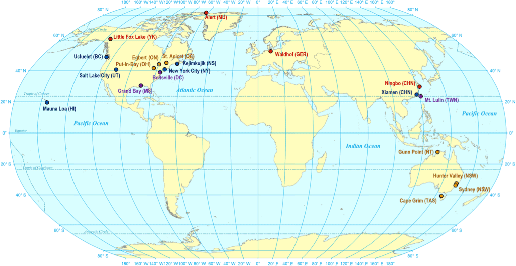
Figure 1Sampling sites for passive air sampler accuracy testing. Sampling sites are coloured by intensity of PAS deployments: high (monthly, seasonal, half yearly, and yearly deployments), medium (seasonal, half yearly, and yearly deployments), low (half yearly and yearly deployments), and very low (yearly deployments).
For this study, PASs and standard operating procedures (see Sect. S1 in the Supplement) were sent from Toronto to 20 sampling sites on four continents (Fig. 1) using Canada Post or international couriers. The PAS were deployed for a period of 1 year at each site during the time between 2015 and 2017. Accessibility of AMNet and ECCC-AMM networks resulted in a greater number of sites in North America than in other global regions. Temporal resolution of sampling ranged from monthly, quarterly, biannual to annual deployments. The number of deployments varied between sites. Four sites with a deployment intensity categorized as “high” were sampled with monthly, quarterly, biannual, and annual resolution. Six “moderate” deployment intensity sites had quarterly, biannual, and annual resolution. Seven “low” deployment intensity sites had biannual and annual resolution and three “very low” deployment intensity sites had year-long deployments. Exact numbers, lengths, and dates of deployments at each site are shown in Tables S2.1, S2.2, and S2.3 in the Supplement. After deployments, PASs were stored at each site until the last PAS had been retrieved, at which point they were returned to Toronto by courier for analysis of the sorbent content. In total, there were 142 triplicated deployments (426 samplers) across all sites. Field blanks were obtained by transporting PASs to each site, removing the Teflon tape and solid cap, attaching an open cap with mesh screen, holding it up to a deployment position for 10 s, and then immediately taking it down, closing, and sealing it as described above. Temperature and wind speed for each deployment period, as recorded by weather stations at or near the sampling sites, are listed in Table S2.3.
2.2 Active air sampling
TGM and GEM concentrations were measured with Tekran 2537 series cold-vapour atomic fluorescence spectrometer (CVAFS) systems. Details of instrument setup are given in Landis et al. (2002), Steffen et al. (2008), Cole et al. (2013), and NADP (2015). Concisely, the instrument consists of a 2 µm Teflon filter (47 mm diameter) at the inlet of a heated sampling line (of variable length; site dependent) and a second filter at the instrument inlet. Australian sites did not use the outer filter or a heated inlet and are therefore likely to only sample GEM. Ambient air is pulled through the sampling line at a flow rate of 1 to 1.5 L min−1 (depending on site and network protocols) with concentrations normalized to the specific rate at each site. Continuous, 5 min resolution concentrations are produced by alternating collection and analysis on one of the two gold traps within the instrument. The analysis phase is initiated by heating a gold trap to ≈ 500 ∘C, releasing the sorbed Hg into pure argon gas, and detecting mercury by atomic florescence spectrometry. Routine internal (permeation source) and external (injections) calibrations were performed at each site. All data were quality controlled using the Research Data Management and Quality Assurance System (RDMQ™; McMillan et al., 2000; Steffen et al., 2012). Differences in sampling methods may result in slight inconsistences in the sampled species among sites.
Tekran 1130 and 1135 speciation units paired with a Tekran 2537 CVAFS were deployed at Alert, Mauna Loa, Salt Lake City, Beltsville, and Grand Bay. Again, full details are provided elsewhere (Landis et al., 2002; Steffen et al., 2008; Cole et al., 2013). In brief, ambient air enters these systems through an impactor inlet (to remove particles > 2.5 µm) before passing through a potassium chloride denuder to trap GOM, a particle filter to collect particulate bound Hg, and finally into the Tekran 2537 for analysis of GEM. The typically low concentrations of GOM and particulate bound Hg require a higher flow rate (10 L min−1) and a lower temporal resolution (1 to 3 h) to collect sufficient analyte for analysis by the Tekran 2537. The GEM component is continuously measured at 5 min resolution in the same manner described for the Tekran 2537 series samplers above. It has been hypothesized that GOM may make a greater proportion of TGM than previously thought (Ambrose et al., 2013; Gustin et al., 2015; Huang et al., 2013b). Nonetheless, the incipient GOM measurement techniques (based on ion exchange membranes or nylon filters) used have produced inconclusive results and, similar to the conventional sampling methodologies (based on particle impact filters and annular denuders), they are subject to sampling artefacts that may skew results (Cheng and Zhang, 2016; Ariya et al., 2015). Thus, the GOM measurements made at these sites using Tekran speciation analyzers may still aid in elucidating whether the samplers sorb solely GEM or TGM.
Information on the percentage data coverage across the deployment periods of the active measurement systems and PASs (successful samples/deployments out of actual samples/deployments) is shown in Table S2.2. The 5 min TGM and GEM data from the Tekran 2537 series instruments or the Tekran 2537 component of the speciation units were compared with the concentrations derived from the PASs. For Alert station, which operates both a Tekran 2537X sampler and a Tekran 1130 or 1135 speciation unit, data from the former were used for comparison.
Given that TGM is generally dominated by GEM at most sites (typically > 95 %; Cole et al., 2014; Driscoll et al., 2013; Rutter et al., 2009; Slemr et al., 2015), differences between the two concentrations are likely to be small. To ensure consistency with the nomenclature used for the PASs, the analyte sampled by non-speciating Tekran 2537 instruments is referred to as gaseous Hg. The PAS-derived concentrations were compared with the speciated data available for Alert, Mauna Loa, Salt Lake City, Beltsville, and Grand Bay to ascertain whether the PASs accumulate GOM.
Mauna Loa (3397 m a.s.l.) and Mt. Lulin (2862 m a.s.l.) are high-altitude sites and required active concentrations to be adjusted for pressure. At Mt. Lulin, to obtain a volumetric flow rate of 10 L min−1, the mass flow rate was lowered by a factor of 0.6900, which is the ratio of the average atmospheric pressures at this site (70.00 kPa) and at sea level (101.325 kPa). The gaseous Hg concentrations reported for Mauna Loa were multiplied by 0.6716, which is the ratio of the mean air pressure during the deployments (68.05 ± 0.04 kPa) and at sea level.
2.3 Data reporting
The uncertainty of all reported values is given by one standard deviation. The standard errors of regression coefficients were also converted to standard deviations. Uncertainties are reported to one significant digit unless the first non-zero digit is a 1, in which case there are two significant digits (e.g. 5.43 ± 0.17; Hughes and Hase, 2010). All data are written with one extra digit beyond the appropriate significant digits to avoid rounding errors when using the PAS in the future. The extra digit is written in subscript (i.e. 0.3450 ± 0.0034 or 5.429 ± 0.17). The exception to the use of the added digit is the reporting of gaseous Hg concentrations, which will follow standard reporting methods used in the atmospheric Hg literature: measurements corrected to the nearest 0.01 ng m−3.
2.4 Analysis for total Hg
All PASs were analyzed at the University of Toronto Scarborough for the total mass of Hg using an AMA254 (Leco Instruments Ltd.) by means of thermal combustion, amalgamation, and atomic absorption spectroscopy in pure oxygen carrier gas (USEPA method 7473; USEPA, 2007). To prevent sulfur poisoning of the instrument's catalyst by the high sulfur sorbent (S = 8–15 wt %), sodium carbonate was added to the end of the catalyst tube (≈ 5 g) and directly on top all analyzed samples, standards, and reference materials (≈ 0.2 g; McLagan et al., 2017a). The entire mass of sorbent in each sample (0.73 ± 0.04 g) was analyzed in two aliquots of up to 0.45 g to remove uncertainty related to the heterogeneity of sorbed Hg throughout the sorbent matrix. During analysis, samples were dried at 200 ∘C for 30 s then combusted at 750 ∘C for 330 s. After reduction by the system catalyst, which was continually heated to 550 ∘C, GEM was trapped on a gold amalgamator. After combustion, a 60 s purge ensured the removal of all pyrolysis gases from the system. Heating the amalgamator to 900 ∘C for 12 s released the trapped Hg into a cuvette where absorption was measured by dual detector cells for high and low absolute amounts of Hg at 253.65 nm wavelength.
The instrument was calibrated via the addition of diluted Hg liquid standard (1000 ± 5 mg L−1; in 10 % w∕w HCl; Inorganic Ventures) to ≈ 0.22 g of clean (unexposed) HGR-AC sorbent. The low and high cells were calibrated using standards of 0, 1, 2.5, 5, 10, 15, and 20 ng and 25, 50, 100, 250, and 500 ng, respectively (uncertainty in autopipette is 1 ± 0.004 ng). As the response is not linear near each cell's upper limit (≈ 20–25 ng for the low cell and 500 ng for the high cell), calibration curves were fitted with quadratic relationships.
Quality assurance and quality control
Analytical blanks, i.e. clean (unexposed) HGR-AC sorbent, were analyzed regularly and had a mean concentration of 0.309 ± 0.147 ng g−1 (n= 33). The mean concentrations in field blanks, i.e. unexposed samplers undergoing the same transport as regular PAS (for detail see Sect. S1), are listed in Table S2.4 for each sampling site. All PAS deployments were blank adjusted by subtracting the mean field blank Hg concentration (ng g−1) at each site multiplied by the mass of HGR-AC in the sample, from the mass of Hg in the sample. Analytical precision was examined by analyzing 5, 10, 50, and 100 ng Hg liquid standards added to ≈ 0.22 g of clean (unexposed) HGR-AC approximately every 10–15 samples. Recoveries of the Hg liquid standards were 99.95 ± 1.1 % (n= 215). Accuracy was monitored via alternating analysis of a high sulfur, bituminous coal standard reference material, NIST 2685c (S = 5 wt %; National Institute of Standards and Technology) and our own in-house reference material RM-HGR-AC1 (powdered HGR-AC sorbent loaded with Hg by exposure to air for 4 months then homogenized; 23.1 ± 0.8 ng g−1 based on 198 analytical runs) approximately every 10–15 samples. Recoveries for the NIST 2685c and RM-HGR-AC1 were 98.4 ± 2.7 % (n= 57) and 98.8 ± 3.6 % (n= 86), respectively.
2.5 Calculation of air concentration from the amount taken up by the PAS
Gaseous Hg concentrations in the atmosphere, C (ng m−3), are calculated from the mass of sorbed Hg, m (ng), according to Eq. (1):
where SR is the sampling rate of the PAS (McLagan et al., 2016b) and t is the deployment time of the sampler (day). In this study, three sets of air concentrations were derived from the measured m. The first set was derived by using the original, published SR of 0.1210 m3 day−1 (hence termed original SR) obtained during a year-long calibration of the PAS on the campus of the University of Toronto Scarborough (McLagan et al., 2016b).
The second set of air concentrations was calculated by using a recalibrated SR obtained from the data generated in this study plus the data from the original calibration experiment (hence termed recalibrated SR). This recalibrated SR was calculated using the slope method as described by Restrepo et al. (2015) and McLagan et al. (2016b). Rearranging Eq. (1), we can derive a SR for individual deployments from the mass of sorbed Hg, m, in a PAS and the gaseous Hg concentration, CA, measured by an active instrument during that PAS's deployment period:
In this method, SR is calculated as the slope of a linear regression of m against (C⋅t).
The third set of air concentrations was calculated using the recalibrated SR with adjustments for the mean temperature, Texp (∘C), and wind speed, WSexp (m s−1) (hence termed adjusted SR), during each deployment using factors previously determined in controlled laboratory experiments (Eq. 3; McLagan et al., 2017b):
where SRcal is the recalibrated SR (m3 day−1).
The three sets of air concentrations derived from the PAS, CPAS (ng m−3), were compared with the actively derived gaseous Hg concentrations, CACT (ng m−3), and in each case a mean normalized difference (MND) was calculated.
where n is the number of comparisons. Deployments were included in the MND calculation if at least one PAS was successfully deployed and analyzed and successful active sampling data covered at least 25 % of the PAS`s deployment period. To determine if passive concentrations were improved by the temperature and wind speed adjusted SR the MND of the recalibrated SR and adjusted SR were compared by means (one-tailed pairwise t test) and variance (Levene's test). For sites with active speciation measurements, MNDs based on active–passive comparisons of GEM and TGM concentration data were compared for both the recalibrated SR and adjusted SR at each site (two-tailed pairwise t test) to determine which data set is a better fit with the passive concentrations. The mean relative standard deviation (RSD; standard deviation divided by the mean multiplied by 100) of replicates from individual deployments was used to assess the precision-based uncertainty of the sampler.
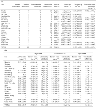
Table 1Mean passive and active air sampler data at each sampling location. (a) Replicate relative standard deviation, uptake rate, original sampling rate (SR), recalibrated SR, and adjusted SR adjusted for the measured temperature and wind speed at each sampling site (Eq. 3). (b) Gaseous Hg concentrations (conc.) and uncertainty (mean normalized error; MND) when calculated with three different sampling rates.
3.1 Replicate precision of the passive air sampler
Few PAS samples were lost during deployment, transport, or analysis. Reasons for losses were poorly sealed samplers, errors in recording of deployment time and dates, loss during analysis (e.g. catalyst failure), and a hail storm (Hunter Valley site). Of 142 triplicated PAS deployments, 93 % (132 deployments, 378 samplers) and 89 % (129 deployments, 375 samplers) had at least one and two successfully analyzed PAS, respectively. The precision-based uncertainty of the PAS calculated from the successful replications was 3.6 ± 3.0 % (Table 1), which is slightly worse than was reported for the original outdoor calibration experiment (2 ± 1 %) in Toronto, Canada (McLagan et al., 2016b). The slight decrease in precision is to be expected as the samplers were deployed by different individuals at each location whose only training were written and video-recorded standard operating procedures (see Sect. S1). Nonetheless, the precision of the sampler remains high, especially in comparison to other PAS for Hg, the best of which had a reported precision of 7.7 % (Skov et al., 2007). Others had deviations between replicates in excess of 10 % or precision was not reported at all (Brown et al., 2012; Gustin et al., 2011; Huang et al., 2012; Zhang et al., 2012). These results confirm the excellent reproducibility that can be achieved with this PAS even when used by newly and informally trained personnel.
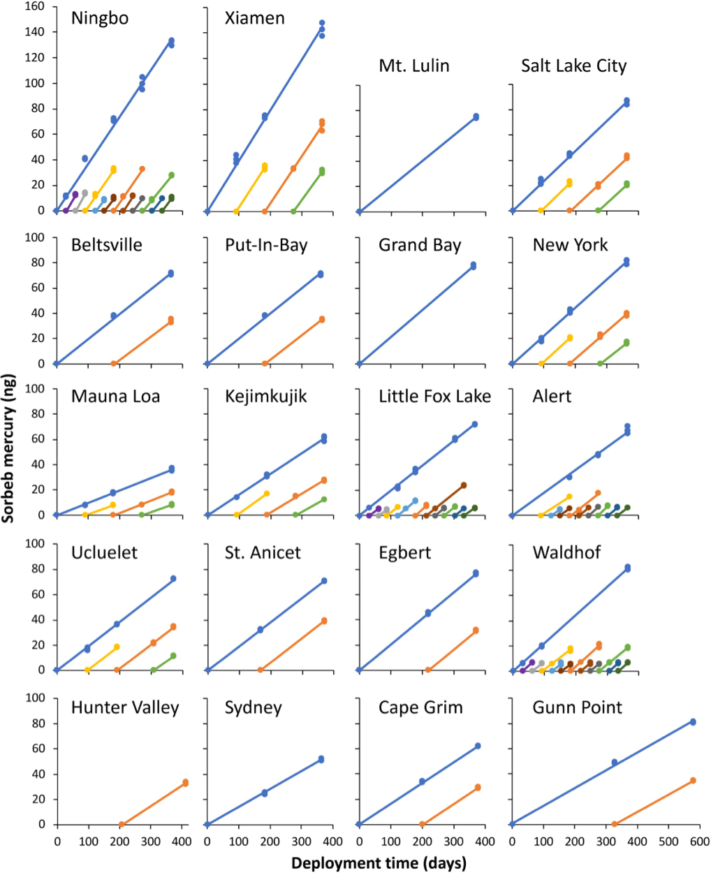
Figure 2Uptake curves and individual deployments of passive air samplers across all 20 sampling locations. 0 ng points mark the beginning of deployments. All samples on the same line are for deployments that began at the same time. All axes are scaled the same. Deployments of the same colour cover equivalent deployments periods (i.e. orange is 7–12-month deployment at all sites).
3.2 Passive air sampler uptake curves
The amount of mercury quantified in each individual sampler is plotted against the deployment time in Fig. 2. These uptake curves are highly linear over 12 months at all sites, confirming that the PASs do not approach a limit to their uptake capacity throughout all deployments. At Xiamen and Ningbo, sites with the highest uptake rates, i.e. the mass of Hg sorbed per unit time, and hence the highest ambient gaseous Hg concentrations (Table 1), 144 and 133 ng of Hg, respectively, were taken up over a 12-month period. This is almost double the mass of Hg taken up in the original uptake experiment (McLagan et al., 2016b) and indicates the maximum deployment time of the sampler is at least 1 year even under the elevated concentrations observed in East Asia. The high uptake capacity of the HGR-AC sorbent for gaseous Hg is due to a large surface area to volume ratio and the affinity of gaseous Hg to the impregnated sulfur (McLagan et al., 2016a; Suresh Kumar Reddy et al., 2013; Zhang et al., 2012).
Uptake rates can be derived from the slopes of the curves in Fig. 2. Uptake rates of PASs deployed at the same site (comparing slopes within each panel in Fig. 2) are very uniform. The greatest relative variability in uptake rate between samples at any one site occurred at Alert (Table 1) and was low (< 25 % RSD; Table 1). This attests to the stability of both (i) the SR and (ii) the gaseous Hg concentrations at each site over the length of the PAS deployments (1 month or longer). The time-averaged nature of the concentrations measured by the PASs conceals much of the variability that generally occurs at shorter time resolution. The higher variability in uptake rates and gaseous Hg concentrations at Alert and Ningbo (Table 1) can be attributed to springtime atmospheric Hg depletion events (Steffen et al., 2008) and seasonal variability in the elevated East Asian background concentrations, respectively. The differences in uptake rates between sites (comparing slopes among different panels in Fig. 2) were caused by different gaseous Hg concentrations at each location as evidenced by the significant correlation between uptake rate and active gaseous Hg concentration data (p < 0.001).
3.3 Sampling rates and differences between active- and passive-derived gaseous Hg concentrations
The Tekran 2537 active monitoring instruments successfully recorded Hg concentrations during 59 % of all deployment periods. Data gaps were caused by instrument failures, power outages, or removal of poor-quality data during RDMQ™ processing. The PASs covered a greater percentage of the deployment periods across all sites, indicating its high reliability and ease of use. A comparison of active and passive sampling was considered meaningful if an active instrument had recorded data during at least a quarter of a PAS's deployment time. This was the case in 113 of 142 deployments (80 %). 107 of these 113 deployments (306 samplers) had at least one successful PAS data point and therefore were used in the comparison of actively and passively derived gaseous Hg concentrations (Table 1). Because the sites in Sydney, Hunter Valley, and Xiamen did not have adequate data coverage for any of the deployments, the comparison included 17 of the 20 total sites.
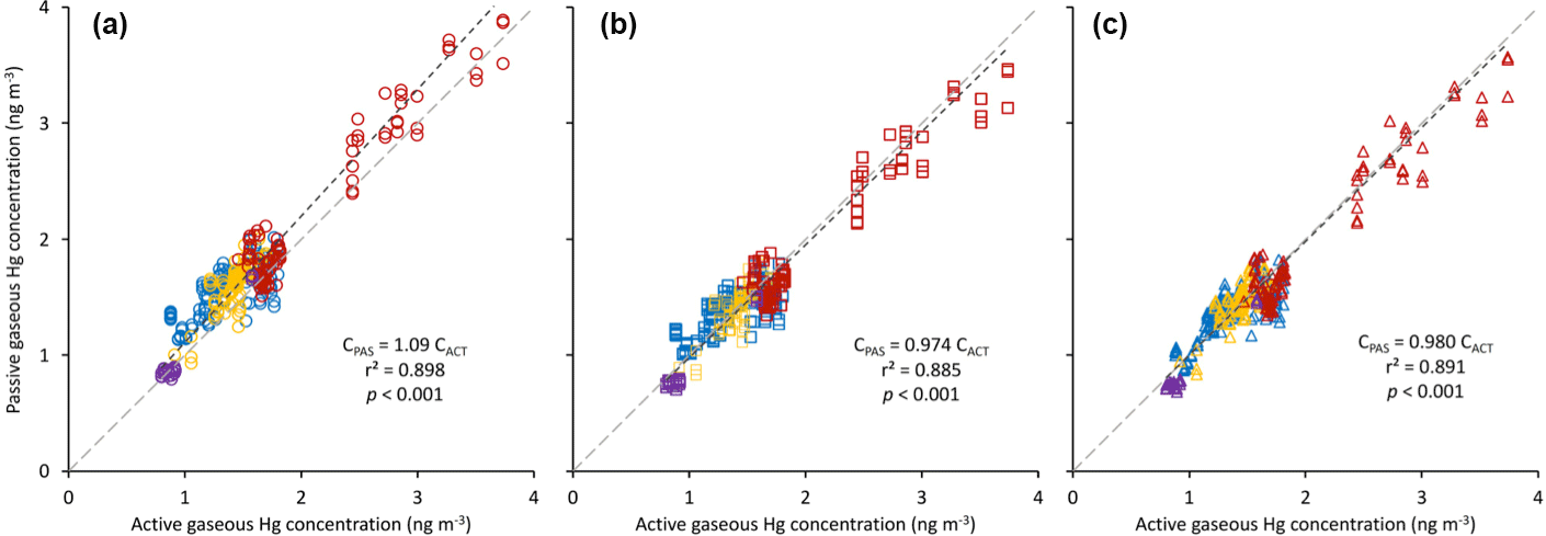
Figure 3Comparison of active (CACT; x axis) and passive (CPAS; y axis) gaseous Hg concentrations derived from the original sampling rate (SR; circles in a), recalibrated SR (squares in b), and adjusted SR (triangles in c). Dotted lines represent the trend line for each dataset. Grey dashed line is the 1:1 relationship. Markers are coloured according to site type: red – urban sites; blue – rural sites; purple – high-altitude sites; and yellow – northern/Arctic sites. Fitted relationships are for all data combined.
The gaseous Hg concentrations calculated from the PAS using the original SR of 0.1210 ± 0.005 m3 day−1 (McLagan et al., 2016b) deviated from the active air concentrations on average by 14.2 ± 10 %. The PASs were, in general, overestimating the gaseous Hg concentrations (most data points and the linear regression line between active and passively determined concentration are above the 1:1 line in Fig. 3a), which suggested the original SR was biased low. Laboratory experiments on the effects of meteorological parameters on the SR also suggested the original SR was low (McLagan et al., 2017b). The original SR was based on only 37 samples at one sampling location in Toronto (McLagan et al., 2016b). The limited data set and range of conditions is the likely reason for much of this bias.
The recalibrated SR based on 343 passive samplers deployed at 17 sites with collocated active samplers (37 samples from McLagan et al., 2016a, and 306 samples from this study) was 0.1354 ± 0.016 m3 day−1 (see Fig. S2.1 in the Supplement for plot of m against C⋅t for all samples). Because of the broad range of latitudes, meteorological conditions, deployment times, and altitudes across these sites, we recommend using the recalibrated SR of 0.1354 ± 0.016 m3 day−1 as the baseline SR for the PAS.
McLagan et al. (2016b) theoretically estimated the SR of the PAS based on the molecular diffusivity of elemental Hg and an estimated effective diffusion distance. Using an air-side boundary layer thickness of 15 mm, which has been recommended for outdoor deployments with the protective shield (McLagan et al., 2016b) and the mean temperature across all deployments in this study (9.89 ∘C), this approach predicts a SR of 0.1306 m3 day−1. This modelled SR is only 3.5 % lower than the recalibrated SR, which provides further confidence in the mechanistic understanding of the uptake process of Hg within this PAS.
When the recalibrated SR is used for the derivation of air concentrations from the PAS, the MND compared to active instrument-derived concentrations is significantly (p < 0.001) reduced to 8.8 ± 7.3 %. When the air concentrations for the PAS are derived using the adjusted SR, the MND is 8.7 ± 5.7 % (Table 1). While this value is not significantly lower than that obtained using the recalibrated SR (p= 0.581), passive and active gaseous Hg concentrations are more highly correlated when the adjusted SRs were applied (r2 reported in Fig. 3). Moreover, the variance in the discrepancy is significantly lower (Levene's test; p= 0.046), which can be linked to smaller discrepancies when the adjusted SR was applied at some of the sites with extreme wind speed and/or temperature conditions. For example, without adjustment the gaseous Hg concentrations at the Cape Grim site were overestimated by the PAS as the recalibrated SR (unadjusted) is too low for the strong westerly wind at this site (mean: 10.2 m s−1 substantially higher than at any other site, Table S2.3). Not surprisingly, at locations with conditions closer to the mean temperature (9.89 ∘C) and wind speed (3.41 m s−1) of the adjusted SR calculation, differences between active and passive sampler-derived concentrations were very similar when the recalibrated SR or the adjusted SR was applied (Table 1). We also calculated gaseous Hg concentrations for the PAS using the recalibrated SR adjusted solely for temperature and solely for wind speed. In neither case did these individually adjusted SRs significantly reduce the discrepancies or their variance (p > 0.05) relative to the use of the unadjusted recalibrated SR.
Additionally, deployment length had no significant effect on the MND of samples for either the recalibrated SR (p= 0.082) or the adjusted SR (p= 0.298). Thus, neither the recalibrated nor adjusted SRs nor the uncertainty of the sampler is dependent upon the length of deployment at background concentrations over deployments lasting 1 to 12 months (Fig. S3.1). Nine-month deployments were not considered in this analysis as there were only two deployments of this length at Alert and Little Fox Lake.
3.4 Placing the PAS performance into context
It is important to acknowledge that this is not a fully independent evaluation of the performance of the sampler, as the same data were used in the derivation of the recalibrated SR and in the determination of the air concentrations from the PAS. However, we stress that data from all sites were used to derive a single recalibrated SR that was used for all sites; i.e. the fitting involved was not site-specific. For example, the Little Fox Lake site contributed the most data points to the recalibration (n= 49), but those data only represented 14 % of the whole data set.
Our precision estimate (3.6 ± 3.0 %), calculated as the average of the standard deviation of the results for replicated deployments of the passive air sampler, is a measure of random error only. Quantifying the systematic error would require knowledge of the true gaseous concentration of mercury during a PAS's deployment. Because that concentration is not known, we instead use the MND between the concentration obtained with the PAS and the Tekran systems as an estimate of the potential systematic uncertainty of the PAS (8.7 ± 5.7 % when the adjusted SR is applied). On the one hand, this MND overestimates the uncertainty of the PAS by attributing all of the discrepancy to it, even though part of the discrepancy is surely attributable to the Tekran. By sampling with two collocated Tekran 2537A instruments, Temme et al. (2007) estimated a measurement uncertainty of 8.8 %. Aspmo et al. (2005) describe the uncertainty of the same system in the range of 5–10 %. Based on a review of several intercomparisons involving Tekran 2537 instruments, Slemr et al. (2015) estimated a systematic uncertainty of ≈ 10 %, but warn this can expand up to 20 % in extreme cases. Even if the Tekran systems were to yield true values of the concentrations, the MND can be partly attributed to data gaps in the active instrument measurements (see Table S2.2) that if successfully analyzed would have altered the active concentration at that site in some way. On the other hand, there is also the possibility that the MND underestimates the systematic error of the PAS, namely if most or all of the Tekran systems in our study were biased similarly low (or high). Because the same TEKRAN data are used for both the sampling rate calibration and the calculation of the MND, this bias would be “inherited” by the PAS and therefore not be apparent in the MND. If, however, some Tekran data are biased high and some are biased low, this would be unlikely to lead to an underestimation of the uncertainty of the PAS.
In summary, we judge the overall uncertainty of the PAS to be higher than the precision based uncertainty (3.6 ± 3.0 %), because of the potential for systematic bias, but also not higher on average than the MND obtained with the adjusted SR (8.7 ± 5.7 %), because that discrepancy is not solely attributable to systematic bias by the PAS. Even this conservative assessment of PAS accuracy is in line with active instruments' uncertainty and qualifies the device as appropriate for background monitoring of gaseous Hg.
The performance of the PAS using either the recalibrated or adjusted SR represents a substantial improvement over all existing gaseous Hg PAS designs to date, especially those with sufficiently low detection limits to monitor background concentrations (as summarized in a review on gaseous Hg PASs by McLagan et al., 2016a). While the accuracy-based uncertainty of the 3M PAS by McCammon and Woodfin (McCammon and Woodfin, 1977) was similar (8 ± 7 %), this device was only tested in the range of 25 000–300 000 ng m−3 gaseous Hg concentrations over an 8 h period, making it unsuitable for background monitoring. Of the PASs that have sufficiently low detection limits to monitor background concentrations the lowest overall uncertainties were 19 ± 14 (Huang et al., 2012) and 22 ± 15 % (Guo et al., 2014; Zhang et al., 2012). Other designs had uncertainties greater than 30 % (Brown et al., 2012; Nishikawa et al., 1999), reported only replicate precision (Brumbaugh et al., 2000; Skov et al., 2007), or reported no uncertainty estimate at all (Gustin et al., 2011).
3.5 Site-specific analysis
Plots comparing active instrument-derived gaseous Hg concentrations with passive concentrations determined using the original, recalibrated, and adjusted SRs for each sampling site are presented in Sect. S4 (Figs. S4.1–S4.17). The data in Fig. 3 are colour coded by site categorization (urban, rural, altitude, northern/Arctic).
3.5.1 Urban sites
Of the 20 sampling locations from the current study, five were classified as urban (Xiamen, Ningbo, Salt Lake City, New York City, and Sydney). Additionally, the previous calibration study site in Toronto was included in recalibrations and uncertainty assessments. Overall, there was good agreement between active and passive concentrations using the recalibrated (MND: 8.5 ± 4.7 %) and adjusted SRs (MND: 8.5 ± 5.2 %) for those five sites. Both Xiamen and Ningbo sites were selected due to the elevated gaseous Hg concentrations typically observed in East Asia (Wan et al., 2009; Xu et al., 2015; Zhu et al., 2012). Unfortunately, the majority of active sampling data at Xiamen and nearly half the data at Ningbo were lost due to active instrument malfunctions, limiting active–passive comparisons to 10 deployments at Ningbo. The mean temperature and wind speed during deployments at this site (Table S2.3) varied little from the mean values across all sites, which resulted in little difference between passive concentrations derived from recalibrated and adjusted SRs (Table 1; Fig. S4.7). The active data recorded in Sydney, Australia, were also insufficient across any of the deployments for comparison with passive concentrations. Mean gaseous Hg concentrations calculated using the adjusted SR for all PAS deployments were 2.53 ± 0.28 in Xiamen and 0.91 ± 0.28 ng m−3 in Sydney.
Salt Lake City may experience elevated GOM concentrations and atmospheric Hg reactivity in general due to the increased presence of atmospheric halogenated species in the atmosphere around the Great Salt Lake (Gay et al., 2013; Peterson and Gustin, 2008; Stutz et al., 2002). Only one of the seven deployments in Salt Lake City had sufficient actively measured speciation data for comparison. The mean GOM concentration for that deployment was 0.014 ng m−3, which represents < 1 % of the mean active GEM concentration for the same period (1.67 ng m−3). Hence, we are unable to use this data to infer the mercury species sampled by the PAS. Discrepancies between active instrument-derived concentrations and concentrations derived using recalibrated and adjusted SRs over this single deployment were not significantly different (p= 0.280).
Concentrations derived from PASs deployed in New York City using recalibrated (8.6 ± 4.6 %) and adjusted SRs (7.7 ± 4.6 %) deviated to a similarly small extent from the active concentrations (p= 0.271; Table 1; Fig. S4.4). While mean temperatures during deployment were higher than the overall mean, wind speeds were lower, cancelling out their respective effects (Table S2.3). Differences between active and passive derived concentrations at Toronto from the previous study were also similar using both recalibrated and adjusted SRs (10.2 ± 4.4 and 10.6 ± 5.2 %, respectively). A full discussion of those results can be found in McLagan et al. (2016b).
Good agreement between active and passive concentrations both at typical hemispheric and elevated East Asian background concentrations using either the recalibrated or adjusted SR (uncertainties not significantly different; p= 0.381) demonstrates that the SRs are not concentration dependent, which is essential for effective gaseous Hg monitoring.
3.5.2 Rural sites
Eleven sites (Beltsville, Put-in-Bay, Grand Bay, Kejimkujik, Ucluelet, St. Anicet, Egbert, Waldhof, Hunter Valley, Cape Grim, and Gunn Point) were located in rural settings. Put-In-Bay is situated on South Bass Island on the Ohio (USA) side of Lake Erie. Temperatures at the site were similar to the mean of all sites, but wind speeds were high. Nonetheless, differences from active concentrations were small using either recalibrated or adjusted SR, i.e. were not significantly reduced by adjusting the SR for wind speed and temperature (p= 0.082). Grand Bay (on the Gulf of Mexico in Mississippi, USA) experiences relatively high temperatures and moderate wind speed (Table S2.3). Using the adjusted SR significantly reduced the discrepancy (p= 0.013) from the active data compared to the use of the recalibrated SR (Fig. S4.2). Two sites are situated in the very north and south of Australia; Gunn Point is a hot, windy location at the top of the Northern Territory and Cape Grim is located on the mild, but exceptionally windy west coast of Tasmania (Table S2.3). Consequently, these more extreme conditions resulted in the calculation of the highest mean adjusted SR values of any of the sites (0.1572 ± 0.0006 and 0.1572 ± 0.0020 m3 day−1, respectively). The concentrations derived from the adjusted SR were substantially reduced relative to those calculated using the recalibrated SR (Figs. S4.9 and S4.10, respectively), which resulted in a significantly better agreement with the active concentrations at both Cape Grim (p < 0.001) and Gunn Point (p= 0.019). Significant improvements in passive concentration data at three of the four sites with high temperatures and/or wind speeds demonstrate the need for adjusting the SR during similar deployments. While there was some seasonal variability in conditions at Beltsville, Kejimkujik, St. Anicet, Ucluelet, and Waldhof, mean temperature and wind speeds at each site were, in general, similar to the mean values for all sites. As such, there were no significant differences between MNDs with either the recalibrated or adjusted SRs (p > 0.05; Table 1; Figs. S4.1, S4.6, S4.13, S4.14, and S4.15, respectively) at these locations.
At both Beltsville and Grand Bay, the proportion of GOM in TGM measurements was < 1 % for all deployments. Hence, no information on the sampled analyte could be derived from these data.
3.5.3 High-altitude sites
The two high-altitude sampling sites at Mt. Lulin and Mauna Loa provided a unique opportunity to not only examine the PAS's functionality under relatively low atmospheric pressure conditions, but also to test its performance in a likely more dynamic zone of atmospheric chemistry at or above the planetary boundary layer (Bieser et al., 2017; Carbone et al., 2016). Lower atmospheric pressure has the potential to affect the PAS in two ways: (i) increasing the SR because diffusivity coefficients are inversely proportional to pressure (Armitage et al., 2013; Klánová et al., 2008; Seethapathy et al., 2008) and (ii) decreasing the SR as there is less mass per volume of air. While the use of mixing ratios would prevent the latter effects, they are not the preferred method of reporting atmospheric Hg measurements (Weigelt et al., 2016). These two effects should theoretically cancel each other out, and hence we would expect passive concentrations to align with pressure-adjusted active concentrations. At Mt. Lulin the MNDs were low for both the recalibrated (5.3 ± 1.2 %) and adjusted (6.7 ± 1.2 %) SRs and not significantly different (p= 0.118; Fig. S4.8). There was also no significant improvement in MND (p= 0.693) using the adjusted SR (12.2 ± 4.6 %) over the recalibrated SR (11.7 ± 4.5 %) at Mauna Loa (Fig. S4.17). While the MNDs were higher at Mauna Loa than at Mt. Lulin, these values are relative to the observed gaseous Hg concentrations, which were low at Mauna Loa (Table 1). In absolute terms, the mean differences between active and recalibrated and adjusted passive concentrations at Mauna Loa were 0.11 ± 0.04 and 0.10 ± 0.04 ng m−3, respectively.
Active GOM concentrations measured by the Tekran speciation unit were elevated at Mauna Loa and made up 9.5 ± 2.9 % of TGM concentrations measured by the same system. Adding GOM concentrations to the 5 min resolution GEM measurements used in the active–passive comparisons significantly increased MNDs for both the recalibrated SR (p < 0.001, TGM: 20.4 ± 2.9 %; GEM: 11.9 ± 4.5 %) and adjusted SR (p < 0.001, TGM: 20.7 ± 2.8 %; GEM: 12.2 ± 2.6 %). These data, considered in isolation, suggest the PAS is not taking up GOM.
3.5.4 Northern/Arctic sites
Two sites from Canada's north were included in the study: Alert (Fig. S4.16), in the high Arctic, and Little Fox Lake (Fig. S4.11), which is north of Whitehorse in the Yukon territory. Both sites had high temporal resolution data, except for the first 4 months of sampling (October to February) at Alert, when PAS data were lost due to poorly sealed samplers and contaminated field blanks. While wind speeds were moderate and not excessively variable across deployments at either site, the mean temperatures of each deployment ranged over 27.4 K at Little Fox Lake and 20.5 K at Alert (Table S2.3). Despite the larger range of temperatures at these sites, mean temperatures across all deployments were not excessively low (Alert: 5.9 ∘C; Little Fox Lake: 2.2 ∘C) as northern summer temperatures were relatively high at both sites. Little Fox Lake, the site with the greatest temperature range, had a significant improvement in the MND using the adjusted SR (p= 0.027), whereas Alert did not (p= 0.454). Although the reduction in MND between active and passive derived concentrations at the northern/Arctic site with the greatest temperature range (Little Fox Lake) highlights the benefit of adjusting SR under extreme conditions, at both sites the MND for either the recalibrated or adjusted SR was low (< 7 %).
The Alert site also employed a Tekran speciation system. The mean GOM concentrations at Alert across the different PAS deployments represented 4.7 ± 6.5 % of the TGM measured by the speciation unit. The high variability in the GOM proportion is associated with springtime atmospheric Hg depletion events; the mean proportion of GOM in TGM was 13.7 ± 13 % during the spring (March, April, and May) deployments. When we consider the data from just these deployments (n= 6) there was no significant difference between MNDs based on the recalibrated SR (p= 0.280; TGM: 14.0 ± 9.3 %; GEM:21.1 ± 12 %) or the adjusted SR (p= 0.140; TGM: 13.7 ± 8.8 %; GEM: 22.8 ± 11 %). When all the data from Alert were considered (n= 36), there again was no significant difference between MNDs based on the recalibrated SR (p= 0.097; TGM: 6.8 ± 6.7 %; GEM: 9.9 ± 8.8 %) or the adjusted SR (p= 0.065; TGM: 7.0 ± 6.0 %; GEM: 10.2 ± 8.4 %). Taken on its own these data cannot confirm whether the PASs are taking up solely GEM or both GEM and GOM (TGM).
From this much larger data set of collocated active and passive measurements of gaseous Hg we were able to revise our original SR, which we determined to be overestimating concentrations, to a recalibrated SR of 0.1354 m−3 day−1. The variability of the maximum uncertainty of the PAS (8.7 ± 5.7 %) was improved by the application of a temperature and wind speed adjusted SR (Eq. 3) recommended by McLagan et al. (2017b). This is in the same range as uncertainties attributed to active measurement instruments (Aspmo et al., 2005; Slemr et al., 2015; Temme et al., 2007) and is unprecedented in gaseous Hg passive air sampling (McLagan et al., 2016a). As such, we recommend the use of the wind- and temperature-adjusted SR but, in the absence of available meteorological data, conclude that the recalibrated SR can be used with a high level of confidence, especially at sites not expected to have excessively high or low temperatures and wind speed. With substantially more data and with very minimal training of personnel, the precision of the instrument remains excellent (3.6 ± 3.0 %). Furthermore, the PASs, with minimal upkeep under some relatively harsh conditions, are considerably less prone than active instruments to issues resulting in data gaps. Overall, results are indicative of the PAS's potential as a tool for monitoring background gaseous Hg concentrations across a wide range of environmental conditions.
This study also attempted to address the exact nature of the analyte being taken up by the sampler. At Mauna Loa, where overall GOM made up the greatest proportion of TGM, PAS results were significantly improved when using active GEM data over TGM data, which agrees with the hypothesis that GOM is removed by the diffusive barrier. Data at Alert were inconclusive as there were no significant differences with the PAS results using either active data for GEM or TGM for either the atmospheric Hg depletion event period or the whole dataset. While the Mauna Loa data do suggest the PAS is taking up solely GEM, the same results were not apparent at Alert, and hence we cannot yet conclude with certainty that GEM is indeed the sole analyte sorbed by the PASs. Furthermore, in all cases, the proportion of GOM (TGM minus GEM) in TGM measurements was close to the level of PAS uncertainty, which further reduces the strength of the conclusions that can be drawn. The deployment of samplers in controlled chambers with a point source of GOM or isotopic analysis of the sorbed Hg may yield more definitive findings.
McLagan et al. (2016a) outlined three key rationales behind the development and use of a gaseous Hg PAS: (i) background concentration monitoring, especially at remote sites, (ii) measuring gaseous Hg gradients with high spatial resolution deployments, and (iii) personal exposure sampling. Results of this study indicate the PAS is a highly precise and accurate tool that can complement and even replace existing monitoring techniques in certain circumstances across the three aforementioned rationales. Additionally, their small size, low cost, non-electrical operation, and applicability across a range of conditions ascribe to their versatility and with consideration may unlock a number of additional deployment scenarios that were not previously viable or even considered with only active monitoring instruments.
All data used in calculations are available in the Supplement. Any additional data can be provided upon request to the corresponding author.
Supplement information includes graphical, written, (linked) video standard operating procedures, all concentration data, and active–passive concentration comparisons for each site.
The supplement related to this article is available online at: https://doi.org/10.5194/acp-18-5905-2018-supplement.
Several of the authors have recently signed a licensing agreement between the University of Toronto and a private corporation concerning the sampler used in the present study. It is possible that this could eventually lead to the commercialization of the sampler.
We would like to sincerely thank all the site technicians and members of AMNET, ECCC-AMM Hg monitoring network, and those at sites outside of these networks that assisted in the deployment
and collection of the PASs and the retrieval and upkeep of active samplers.
These individuals are Dylan Nordin, Rob Tordon, Martin Pilote, Corrine Schiller, Helena Dryfhout-Clark, Kevin Rawlings, Melody Fraser,
Matthew Hirsch, Ronald Cole, Justin Chaffin, Andy Hale, Larry Scrapper, Nash Kobayashi, Da-Wei Lin, and JinSheng Chen. We also acknowledge funding from
Strategic Project Grant no. 463265-14 by the Natural Sciences and
Engineering Research Council of Canada (NSERC) and an NSERC Alexander Graham
Bell Canada Graduate Scholarship. Alexandra Steffen acknowledges funding
from the Northern Contaminants Program of Indigenous and Northern Affairs
Canada for atmospheric Hg monitoring at Alert and Little Fox Lake.
Edited by: Aurélien Dommergue
Reviewed by: three anonymous referees
Ambrose, J. L., Lyman, S. N., Huang, J., Gustin, M. S., and Jaffe, D. A.: Fast time resolution oxidized mercury measurements during the Reno Atmospheric Mercury Intercomparison Experiment (RAMIX), Environ. Sci. Technol., 47, 7285–7294, 2013.
Ariya, P. A., Amyot, M., Dastoor, A., Deeds, D., Feinberg, A., Kos, G., Poulain, A., Ryjkov, A., Semeniuk, K., and Subir, M.: Mercury physicochemical and biogeochemical transformation in the atmosphere and at atmospheric interfaces: A review and future directions, Chem. Rev., 115, 3760–3802, 2015.
Armitage, J. M., Hayward, S. J., and Wania, F.: Modeling the uptake of neutral organic chemicals on XAD passive air samplers under variable temperatures, external wind speeds and ambient air concentrations (PAS-SIM), Environ. Sci. Technol., 47, 13546–13554, 2013.
Aspmo, K., Gauchard, P.-A., Steffen, A., Temme, C., Berg, T., Bahlmann, E., Banic, C., Dommergue, A., Ebinghaus, R., and Ferrari, C.: Measurements of atmospheric mercury species during an international study of mercury depletion events at Ny-Ålesund, Svalbard, spring 2003. How reproducible are our present methods?, Atmos. Environ., 39, 7607–7619, 2005.
Bieser, J., Slemr, F., Ambrose, J., Brenninkmeijer, C., Brooks, S., Dastoor, A., DeSimone, F., Ebinghaus, R., Gencarelli, C. N., Geyer, B., Gratz, L. E., Hedgecock, I. M., Jaffe, D., Kelley, P., Lin, C.-J., Jaegle, L., Matthias, V., Ryjkov, A., Selin, N. E., Song, S., Travnikov, O., Weigelt, A., Luke, W., Ren, X., Zahn, A., Yang, X., Zhu, Y., and Pirrone, N.: Multi-model study of mercury dispersion in the atmosphere: vertical and interhemispheric distribution of mercury species, Atmos. Chem. Phys., 17, 6925–6955, https://doi.org/10.5194/acp-17-6925-2017, 2017.
Brown, R. J. C., Burdon, M. K., Brown, A. S., and Kim, K.-H.: Assessment of pumped mercury vapour adsorption tubes as passive samplers using a micro-exposure chamber, J. Environ. Monitor., 14, 2456–2463, 2012.
Brumbaugh, W. G., Petty, J. D., May, T. W., and Huckins, J. N.: A passive integrative sampler for mercury vapor in air and neutral mercury species in water, Chemosphere, 2, 1–9, 2000.
Carbone, F., Gencarelli, C. N., and Hedgecock, I. M.: Lagrangian statistics of mesoscale turbulence in a natural environment: The Agulhas return current, Phys. Rev. E, 94, 063101, https://doi.org/10.1103/PhysRevE.94.063101, 2016.
Cheng, I. and Zhang, L.: Uncertainty Assessment of Gaseous Oxidized Mercury Measurements Collected by Atmospheric Mercury Network, Environ. Sci. Technol., 855–862, https://doi.org/10.1021/acs.est.6b04926, 2016.
Cole, A. S., Steffen, A., Pfaffhuber, K. A., Berg, T., Pilote, M., Poissant, L., Tordon, R., and Hung, H.: Ten-year trends of atmospheric mercury in the high Arctic compared to Canadian sub-Arctic and mid-latitude sites, Atmos. Chem. Phys., 13, 1535–1545, https://doi.org/10.5194/acp-13-1535-2013, 2013.
Cole, A. S., Steffen, A., Eckley, C. S., Narayan, J., Pilote, M., Tordon, R., Graydon, J. A., St Louis, V. L., Xu, X., and Branfireun, B. A.: A Survey of Mercury in Air and Precipitation across Canada: Patterns and Trends, Atmosphere, 5, 635–668, 2014.
Corbitt, E. S., Jacob, D. J., Holmes, C. D., Streets, D. G., and Sunderland, E. M.: Global source–receptor relationships for mercury deposition under present-day and 2050 emissions scenarios, Environ. Sci. Technol., 45, 10477–10484, 2011.
Driscoll, C. T., Mason, R. P., Chan, H. M., Jacob, D. J., and Pirrone, N.: Mercury as a global pollutant: sources, pathways, and effects, Environ. Sci. Technol., 47, 4967–4983, 2013.
Gay, D. A., Schmeltz, D., Prestbo, E., Olson, M., Sharac, T., and Tordon, R.: The Atmospheric Mercury Network: measurement and initial examination of an ongoing atmospheric mercury record across North America, Atmos. Chem. Phys., 13, 11339–11349, https://doi.org/10.5194/acp-13-11339-2013, 2013.
Guo, H., Lin, H., Zhang, W., Deng, C., Wang, H., Zhang, Q., Shen, Y., and Wang, X.: Influence of meteorological factors on the atmospheric mercury measurement by a novel passive sampler, Atmos. Environ., 97, 310–315, 2014.
Gustin, M. S., Lyman, S. N., Kilner, P., and Prestbo, E.: Development of a passive sampler for gaseous mercury, Atmos. Environ., 45, 5805–5812, 2011.
Gustin, M. S., Amos, H. M., Huang, J., Miller, M. B., and Heidecorn, K.: Measuring and modeling mercury in the atmosphere: a critical review, Atmos. Chem. Phys., 15, 5697–5713, https://doi.org/10.5194/acp-15-5697-2015, 2015.
Herkert, N. J., Spak, S. N., Smith, A., Schuster, J. K., Harner, T., Martinez, A., and Hornbuckle, K. C.: Calibration and evaluation of PUF-PAS sampling rates across the Global Atmospheric Passive Sampling (GAPS) network, Environ. Sci. Process. Impact., https://doi.org/10.1039/C7EM00360A, 2018.
Horowitz, H. M., Jacob, D. J., Zhang, Y., Dibble, T. S., Slemr, F., Amos, H. M., Schmidt, J. A., Corbitt, E. S., Marais, E. A., and Sunderland, E. M.: A new mechanism for atmospheric mercury redox chemistry: implications for the global mercury budget, Atmos. Chem. Phys., 17, 6353–6371, https://doi.org/10.5194/acp-17-6353-2017, 2017.
Huang, J., Choi, H.-D., Landis, M. S., and Holsen, T. M.: An application of passive samplers to understand atmospheric mercury concentration and dry deposition spatial distributions, J. Environ. Monitor., 14, 2976–2982, https://doi.org/10.1039/c2em30514c, 2012.
Huang, J., Miller, M. B., Weiss-Penzias, P., and Gustin, M. S.: Comparison of gaseous oxidized Hg measured by KCl-coated denuders, and nylon and cation exchange membranes, Environ. Sci. Technol., 47, 7307–7316, https://doi.org/10.1021/es4012349, 2013.
Huang, J., Lyman, S. N., Hartman, J. S., and Gustin, M. S.: A review of passive sampling systems for ambient air mercury measurements, Environ. Sci. Process. Impact., 16, 374–392, https://doi.org/10.1039/C3EM00501A, 2014.
Hughes, I. and Hase, T.: Measurements and their uncertainties: a practical guide to modern error analysis, Oxford University Press, 2010.
Klánová, J., Èupr, P., Kohoutek, J., and Harner, T.: Assessing the Influence of Meteorological Parameters on the Performance of Polyurethane Foam-Based Passive Air Samplers, Environ. Sci. Technol., 42, 550–555, 2008.
Landis, M. S., Stevens, R. K., Schaedlich, F., and Prestbo, E. M.: Development and characterization of an annular denuder methodology for the measurement of divalent inorganic reactive gaseous mercury in ambient air, Environ. Sci. Technol., 36, 3000–3009, 2002.
Li, J. and Lee, S. M.: Progress of Global Atmospheric Mercury Field Observations, J. Clean Energ. Technol., 2, 252–258, https://doi.org/10.7763/JOCET.2014.V2.135, 2014.
Lin, C.-J., Pongprueksa, P., Lindberg, S. E., Pehkonen, S. O., Byun, D., and Jang, C.: Scientific uncertainties in atmospheric mercury models I: model science evaluation, Atmos. Environ., 40, 2911–2928, 2006.
McCammon, C. S. and Woodfin, J. W.: An evaluation of a passive monitor for mercury vapor, Am. Ind. Hyg. Assoc. J., 38, 378–386, 1977.
McLagan, D. S., Mazur, M. E. E., Mitchell, C. P. J., and Wania, F.: Passive air sampling of gaseous elemental mercury: a critical review, Atmos. Chem. Phys., 16, 3061–3076, https://doi.org/10.5194/acp-16-3061-2016, 2016a.
McLagan, D. S., Mitchell, C. P. J., Huang, H., Lei, Y. D., Cole, A. S., Steffen, A., Hung, H., and Wania, F.: A High-Precision Passive Air Sampler for Gaseous Mercury, Environ. Sci. Tech. Let., 3, 24–29, 2016b.
McLagan, D. S., Huang, H., Lei, Y. D., Wania, F., and Mitchell, C. P. J.: Application of sodium carbonate prevents sulphur poisoning of catalysts in automated total mercury analysis, Spectrochim. Acta B, 133, 60–62, 2017a.
McLagan, D. S., Mitchell, C. P. J., Huang, H., Abdul Hussain, B., Lei, Y. D., and Wania, F.: The effects of meteorological parameters and diffusive barrier reuse on the sampling rate of a passive air sampler for gaseous mercury, Atmos. Meas. Tech., 10, 3651–3660, https://doi.org/10.5194/amt-10-3651-2017, 2017b.
McMillan, A., MacIver, D., and Sukloff, W.: Atmospheric environmental information – an overview with Canadian examples, Environ. Modell. Softw., 15, 245–248, 2000.
NADP: Atmospheric Mercury Network (AMNet) Site Operations Manual, Version 1.2, National Atmospheric Deposition Network (NADP), available at: http://nadp.sws.uiuc.edu/lib/manuals/AMNet_Operations_Manual_v1-4.pdf (last access: 23 April 2018), Champaign, USA, 2015.
Nishikawa, M., Shiraishi, H., Yanase, R., and Tanida, K.: Examination of an improved passive sampler for gaseous mercury on the landfill site, J. Environ. Chem., 9, 681–684, 1999.
Peterson, C. and Gustin, M.: Mercury in the air, water and biota at the Great Salt Lake (Utah, USA), Sci. Total Environ., 405, 255–268, 2008.
Pirrone, N., Aas, W., Cinnirella, S., Ebinghaus, R., Hedgecock, I. M., Pacyna, J., Sprovieri, F., and Sunderland, E. M.: Toward the next generation of air quality monitoring: mercury, Atmos. Environ., 80, 599–611, 2013.
Pozo, K., Harner, T., Wania, F., Muir, D. C. G., Jones, K. C., and Barrie, L. A.: Toward a Global Network for Persistent Organic Pollutants in Air:? Results from the GAPS Study, Environ. Sci. Technol., 40, 4867–4873, 2006.
Restrepo, A. R., Hayward, S. J., Armitage, J. M., and Wania, F.: Evaluating the PAS-SIM model using a passive air sampler calibration study for pesticides, Environ. Sci. Process. Impacts, 17, 1228–1237, 2015.
Rutter, A. P., Snyder, D. C., Stone, E. A., Schauer, J. J., Gonzalez-Abraham, R., Molina, L. T., Márquez, C., Cárdenas, B., and de Foy, B.: In situ measurements of speciated atmospheric mercury and the identification of source regions in the Mexico City Metropolitan Area, Atmos. Chem. Phys., 9, 207–220, https://doi.org/10.5194/acp-9-207-2009, 2009.
Schroeder, W. H. and Munthe, J.: Atmospheric mercury – an overview, Atmos. Environ., 32, 809–822, 1998.
Seethapathy, S., Górecki, T., and Li, X.: Passive sampling in environmental analysis, J. Chromatogr. A, 1184, 234–253, 2008.
Selin, N. E.: Global biogeochemical cycling of mercury: a review, Annu. Rev. Env. Resour., 34, 43–63, 2009.
Shah, V., Jaeglé, L., Gratz, L. E., Ambrose, J. L., Jaffe, D. A., Selin, N. E., Song, S., Campos, T. L., Flocke, F. M., Reeves, M., Stechman, D., Stell, M., Festa, J., Stutz, J., Weinheimer, A. J., Knapp, D. J., Montzka, D. D., Tyndall, G. S., Apel, E. C., Hornbrook, R. S., Hills, A. J., Riemer, D. D., Blake, N. J., Cantrell, C. A., and Mauldin III, R. L.: Origin of oxidized mercury in the summertime free troposphere over the southeastern US, Atmos. Chem. Phys., 16, 1511–1530, https://doi.org/10.5194/acp-16-1511-2016, 2016.
Shunthirasingham, C., Oyiliagu, C. E., Cao, X., Gouin, T., Wania, F., Lee, S.-C., Pozo, K., Harner, T., and Muir, D. C.: Spatial and temporal pattern of pesticides in the global atmosphere, J. Environ. Monitor., 12, 1650–1657, 2010.
Skov, H., Sørensen, B. T., Landis, M. S., Johnson, M. S., Sacco, P., Goodsite, M. E., Lohse, C., and Christiansen, K. S.: Performance of a new diffusive sampler for Hg0 determination in the troposphere, Environ. Chem., 4, 75–80, 2007.
Slemr, F., Angot, H., Dommergue, A., Magand, O., Barret, M., Weigelt, A., Ebinghaus, R., Brunke, E.-G., Pfaffhuber, K. A., Edwards, G., Howard, D., Powell, J., Keywood, M., and Wang, F.: Comparison of mercury concentrations measured at several sites in the Southern Hemisphere, Atmos. Chem. Phys., 15, 3125–3133, https://doi.org/10.5194/acp-15-3125-2015, 2015.
Sprovieri, F., Pirrone, N., Bencardino, M., D'Amore, F., Angot, H., Barbante, C., Brunke, E.-G., Arcega-Cabrera, F., Cairns, W., Comero, S., Diéguez, M. D. C., Dommergue, A., Ebinghaus, R., Feng, X. B., Fu, X., Garcia, P. E., Gawlik, B. M., Hageström, U., Hansson, K., Horvat, M., Kotnik, J., Labuschagne, C., Magand, O., Martin, L., Mashyanov, N., Mkololo, T., Munthe, J., Obolkin, V., Ramirez Islas, M., Sena, F., Somerset, V., Spandow, P., Vardè, M., Walters, C., Wängberg, I., Weigelt, A., Yang, X., and Zhang, H.: Five-year records of mercury wet deposition flux at GMOS sites in the Northern and Southern hemispheres, Atmos. Chem. Phys., 17, 2689–2708, https://doi.org/10.5194/acp-17-2689-2017, 2017.
Steffen, A., Douglas, T., Amyot, M., Ariya, P., Aspmo, K., Berg, T., Bottenheim, J., Brooks, S., Cobbett, F., Dastoor, A., Dommergue, A., Ebinghaus, R., Ferrari, C., Gardfeldt, K., Goodsite, M. E., Lean, D., Poulain, A. J., Scherz, C., Skov, H., Sommar, J., and Temme, C.: A synthesis of atmospheric mercury depletion event chemistry in the atmosphere and snow, Atmos. Chem. Phys., 8, 1445–1482, https://doi.org/10.5194/acp-8-1445-2008, 2008.
Steffen, A., Scherz, T., Olson, M., Gay, D., and Blanchard, P.: A comparison of data quality control protocols for atmospheric mercury speciation measurements, J. Environ. Monitor., 14, 752–765, 2012.
Stutz, J., Ackermann, R., Fast, J. D., and Barrie, L.: Atmospheric reactive chlorine and bromine at the Great Salt Lake, Utah, Geophys. Res. Lett., 29, 18.1–18.4, https://doi.org/10.1029/2002GL014812, 2002.
Suresh Kumar Reddy, K., Al Shoaibi, A., and Srinivasakannan, C.: Elemental mercury adsorption on sulfur-impregnated porous carbon – A review, Environ. Technol., 35, 1–9, 2013.
Temme, C., Blanchard, P., Steffen, A., Banic, C., Beauchamp, S., Poissant, L., Tordon, R., and Wiens, B.: Trend, seasonal and multivariate analysis study of total gaseous mercury data from the Canadian atmospheric mercury measurement network (CAMNet), Atmos. Environ., 41, 5423–5441, 2007.
Travnikov, O., Angot, H., Artaxo, P., Bencardino, M., Bieser, J., D'Amore, F., Dastoor, A., De Simone, F., Diéguez, M. D. C., Dommergue, A., Ebinghaus, R., Feng, X. B., Gencarelli, C. N., Hedgecock, I. M., Magand, O., Martin, L., Matthias, V., Mashyanov, N., Pirrone, N., Ramachandran, R., Read, K. A., Ryjkov, A., Selin, N. E., Sena, F., Song, S., Sprovieri, F., Wip, D., Wängberg, I., and Yang, X.: Multi-model study of mercury dispersion in the atmosphere: atmospheric processes and model evaluation, Atmos. Chem. Phys., 17, 5271–5295, https://doi.org/10.5194/acp-17-5271-2017, 2017.
UNEP: Minamata Convention on Mercury: Text and Annexes, United Nations Environmental Programme, Geneva, Switzerland, 67, 2013.
USEPA: Method 7473: Mercury in solids and solutions by thermal decomposition, amalgamation, and atomic absorption spectrophotometry, United States Environmental Protection Agency, Washington, 17, 2007.
Wan, Q., Feng, X., Lu, J., Zheng, W., Song, X., Han, S., and Xu, H.: Atmospheric mercury in Changbai Mountain area, northeastern China I. The seasonal distribution pattern of total gaseous mercury and its potential sources, Environ. Res., 109, 201–206, 2009.
Weigelt, A., Ebinghaus, R., Pirrone, N., Bieser, J., Bödewadt, J., Esposito, G., Slemr, F., van Velthoven, P. F. J., Zahn, A., and Ziereis, H.: Tropospheric mercury vertical profiles between 500 and 10 000 m in central Europe, Atmos. Chem. Phys., 16, 4135–4146, https://doi.org/10.5194/acp-16-4135-2016, 2016.
Xu, L., Chen, J., Yang, L., Niu, Z., Tong, L., Yin, L., and Chen, Y.: Characteristics and sources of atmospheric mercury speciation in a coastal city, Xiamen, China, Chemosphere, 119, 530–539, 2015.
Zhang, W., Tong, Y., Hu, D., Ou, L., and Wang, X.: Characterization of atmospheric mercury concentrations along an urban–rural gradient using a newly developed passive sampler, Atmos. Environ., 47, 26–32, 2012.
Zhu, J., Wang, T., Talbot, R., Mao, H., Hall, C. B., Yang, X., Fu, C., Zhuang, B., Li, S., Han, Y., and Huang, X.: Characteristics of atmospheric Total Gaseous Mercury (TGM) observed in urban Nanjing, China, Atmos. Chem. Phys., 12, 12103–12118, https://doi.org/10.5194/acp-12-12103-2012, 2012.
Subscripted numbers are not significant, but are reported to reduce rounding errors in subsequent studies (see Sect. 2.3 for details).