the Creative Commons Attribution 4.0 License.
the Creative Commons Attribution 4.0 License.
 | 12 Dec 2018
Comprehensive organic emission profiles for gasoline, diesel, and gas-turbine engines including intermediate and semi-volatile organic compound emissions
Quanyang Lu
Yunliang Zhao
Emissions from mobile sources are important contributors to both primary and secondary organic aerosols (POA and SOA) in urban environments. We compiled recently published data to create comprehensive model-ready organic emission profiles for on- and off-road gasoline, gas-turbine, and diesel engines. The profiles span the entire volatility range, including volatile organic compounds (VOCs, effective saturation concentration –1011 µg m−3), intermediate-volatile organic compounds (IVOCs, –106 µg m−3), semi-volatile organic compounds (SVOCs, –102 µg m−3), low-volatile organic compounds (LVOCs, µg m−3) and non-volatile organic compounds (NVOCs). Although our profiles are comprehensive, this paper focuses on the IVOC and SVOC fractions to improve predictions of SOA formation. Organic emissions from all three source categories feature tri-modal volatility distributions (“by-product” mode, “fuel” mode, and “lubricant oil” mode). Despite wide variations in emission factors for total organics, the mass fractions of IVOCs and SVOCs are relatively consistent across sources using the same fuel type, for example, contributing 4.5 % (2.4 %–9.6 % as 10th to 90th percentiles) and 1.1 % (0.4 %–3.6 %) for a diverse fleet of light duty gasoline vehicles tested over the cold-start unified cycle, respectively. This consistency indicates that a limited number of profiles are needed to construct emissions inventories. We define five distinct profiles: (i) cold-start and off-road gasoline, (ii) hot-operation gasoline, (iii) gas-turbine, (iv) traditional diesel and (v) diesel-particulate-filter equipped diesel. These profiles are designed to be directly implemented into chemical transport models and inventories. We compare emissions to unburned fuel; gasoline and gas-turbine emissions are enriched in IVOCs relative to unburned fuel. The new profiles predict that IVOCs and SVOC vapour will contribute significantly to SOA production. We compare our new profiles to traditional source profiles and various scaling approaches used previously to estimate IVOC emissions. These comparisons reveal large errors in these different approaches, ranging from failure to account for IVOC emissions (traditional source profiles) to assuming source-invariant scaling ratios (most IVOC scaling approaches).
- Article
(4101 KB) - Full-text XML
-
Supplement
(1587 KB) - BibTeX
- EndNote


Atmospheric particulate matter imposes health risks (Di et al., 2017) and influences climate (Kanakidou et al., 2005). Organic aerosol (OA) contributes 20 %–90 % of submicron atmospheric fine particulate matter mass (Jimenez et al., 2009). OA is commonly classified as primary OA (POA), which is directly emitted by sources, or secondary OA (SOA), which is formed in the atmosphere through photo-oxidation gas-phase organics. Both POA and SOA concentrations depend on the gas-particle partitioning of a complex mixture of organics that span a broad range of volatility (Hallquist et al., 2009; Kroll and Seinfeld, 2008). Mobile sources contribute about one-third of the anthropogenic organic emissions in the 2014 EPA National Emission Inventory (NEI); they are an important source of POA and SOA precursor gases especially in urban environments (Gentner et al., 2017; USEPA-OAQPS, 2015).
Traditional emissions inventories such as the NEI account for emissions of gas-phase volatile organic compounds (VOCs, typically smaller than C12) and non-volatile particulate matter (PM). These emissions are speciated for use in chemical transport models using source-specific emission profiles. Robinson et al. (2007) and Shrivastava et al. (2008) argued that this is an overly simplistic representation of organic emissions.
First, multiple studies have demonstrated that a large fraction of POA is semi-volatile with dynamic gas-particle partitioning while traditional inventories and models treat it as non-volatile (Fujitani et al., 2012; Kuwayama et al., 2015; Li et al., 2016; May et al., 2013a, b, c; Robinson et al., 2007). Semi-volatile POA concentrations depend on the gas-particle partitioning of the emissions, which is determined by their volatility distribution and atmospheric conditions. In addition, source tests are often conducted at unrealistically high OA loading, which biases POA emission factor compared to more dilute, atmospheric conditions (Fujitani et al., 2012; Lipsky and Robinson, 2006). Second, most traditional inventories do not account for emissions of lower volatility organic gases, including intermediate-volatile organic compounds (IVOCs, effective saturation concentration –106 µg m−3) and semi-volatile organic compounds (SVOCs, –102 µg m−3). Laboratory experiments indicate that IVOCs and SVOCs form SOA efficiently (Chan et al., 2009; Presto et al., 2010), but quantifying their emissions requires sorbents which are not routinely used for source testing (Kishan et al., 2008). Neglecting SOA production from IVOCs and SVOCs can lead to substantial underprediction of atmospheric SOA production (Hodzic et al., 2010; Woody et al., 2016). The net effect of these two issues is to cause chemical transport models to overestimate POA emissions and underestimate SOA production, leading to errors in the predicted OA composition and concentrations (Baker et al., 2015; Ensberg et al., 2014; Woody et al., 2016). Accounting for these two issues improves model-measurement agreement (Jathar et al., 2017; Murphy et al., 2017; Woody et al., 2016).
IVOC and SVOC emissions have not been routinely implemented in models because of lack of the mass and chemical composition of total IVOCs and SVOCs (Shrivastava et al., 2008). Although many studies report emissions of individual IVOC and SVOC species (typically polycyclic aromatic hydrocarbon or n-alkanes) (Schauer et al., 1999a, b, 2002; Siegl et al., 1999; Zielinska et al., 1996), the vast majority of the IVOC/SVOC mass cannot be resolved at the molecular level using traditional gas-chromatography-based techniques (Goldstein and Galbally, 2007; Zhao et al., 2014).
Recent studies have reported comprehensive IVOC, SVOC and/or low-volatile organic compound (LVOC, µg m−3) emissions and gas-particle partitioning on POA emissions from mobile sources (May et al., 2014; Presto et al., 2011; Zhao et al., 2015, 2016). Zhao et al. (2015, 2016) characterized the total emissions and chemical composition of IVOCs and SVOCs from a fleet of on- and off-road gasoline and diesel sources. Cross et al. (2013, 2015) reported total IVOC and/or SVOC emission from an aircraft and diesel engine. Presto et al. (2011) and Drozd et al. (2012) reported IVOC and SVOC emissions for two gas-turbine engines. Gentner et al. (2012) and Isaacman et al. (2012a) report molecular and mass spectrum information for IVOC and SVOC in liquid fuel and quartz filter samples. May et al. (2013a, b), Kuwayama et al. (2015), and Li et al. (2016) also investigated the gas-particle partitioning of on-road vehicle POA in dynamometer and tunnel studies. However, only limited comparisons have been made between source categories and the data have not been compiled into model ready profiles.
In this paper, we report comprehensive organic emission profiles for mobile sources by integrating recently published data of organic emissions based on their volatility, including IVOCs and SVOCs, to improve model predictions of SOA formation. We compare our new profiles to traditional source profiles and unburned fuel, focusing on the volatility distribution and SOA precursors. We then use the new profiles to evaluate different scaling approaches previously used to incorporate IVOC emissions into inventories and models. Finally, we present box model calculations of SOA formation to demonstrate the importance to implement the new profiles in SOA modelling.
2.1 Datasets
This paper combines previously published measurement data of organic emissions (Gordon et al., 2013; May et al., 2014; Presto et al., 2011; Zhao et al., 2015, 2016) from gasoline, gas-turbine and diesel engines to create comprehensive model-ready source profiles. All tests used the same procedures to characterize IVOC and SVOC emissions to create a self-consistent dataset for low-volatile organics, but slightly different sampling media (Tedlar bags and/or canisters) and levels of speciation were used to characterize VOC emissions. In the results and discussion sections, we compare these data to other recently published measurements made using different techniques.
We present two types of data: (i) emission factors of total organics and (ii) speciation profiles. We present total organic emissions factors for all tested engines: 64 gasoline vehicles, 5 diesel trucks, 6 off-road gasoline engines, 1 off-road diesel engine and 1 gas-turbine engine. We define total organic emissions as the sum of non-methane organic gases (NMOGs) measured by flame ionization detection plus 1.2 times organic carbon (OC) measured using thermal optical analysis of a quartz filter sample (the factor of 1.2 is the organic-mass-to-organic-carbon ratio, which accounts for the contribution of non-carbonaceous species in the organic, Turpin and Lim, 2001). We define the NMOG as THC (measured with FID) minus CH4 plus carbonyls. We define POA as organics collected by a bare quartz filter analysed by thermal–optical analysis. We converted measured pollutant concentrations to fuel-based emission factors (EF, mg kg−1 fuel) using the carbon-mass-balance approach and the measured mass fraction of carbon in fuel (0.82 for gasoline, 0.86 for jet fuel and 0.85 for diesel) (May et al., 2014; Presto et al., 2011).
We derive speciation profiles from gas-chromatography-based analyses of filter, adsorbent tubes and Tedlar bag/canister samples. Details on the analytical procedures are described by Zhao et al. (2015, 2016). The speciation profiles are based the subset of tests with complete data (all three media): VOCs, IVOCs, SVOCs, and LVOCs. This included 29 gasoline vehicles, 4 diesel trucks, 3 off-road gasoline engines, 1 off-road diesel engine and 1 gas-turbine engine (Table S1 in the Supplement). A detailed description of experimental set-up, sampling and chemical analysis is provided in the original articles (Gordon et al., 2013; May et al., 2014; Presto et al., 2011; Zhao et al., 2015, 2016). Only a brief description is provided here.
Emissions samples were collected from diluted exhaust. Gasoline and diesel source emissions were collected from a constant volume sampler (CVS) that diluted the exhaust with ambient air treated by high-efficient particulate air (HEPA) filters (Gordon et al., 2013; May et al., 2014). Gas-turbine engine exhaust was sampled from a rake inlet installed 1 m downstream of the engine exit plane (Presto et al., 2011). Sources were tested using standard test cycles (Gordon et al., 2013; May et al., 2014; Presto et al., 2011). On-road gasoline vehicles were tested on both cold-start and hot-start unified cycles. On-road diesel vehicles were tested in both lower-speed (creep and idle) and high-speed operation modes. Gas-turbine engine was operated on 4 % and 85 % engine thrust. Off-road engines were operated on certification cycles.
A suite of complementary sampling media was employed to characterize emissions across the entire volatility range. Tedlar bags (for gasoline and diesel sources) or canisters (for the gas-turbine source) were collected and analysed by GC-FID and GC-MS to determine CH4 and VOC hydrocarbon emissions up to C12 compounds (May et al., 2014; Presto et al., 2011). Carbonyls (up to C6) were sampled using 2,4-dinitrophenylhydrazine (DNPH) impregnated cartridges and analysed by high-performance liquid chromatography (HPLC) (May et al., 2014). Quartz filters followed by two Tenax TA adsorbent tubes collected low-volatility organics that were analysed by GC-MS equipped with a thermal desorption and injection system (Gerstel) (Zhao et al., 2015, 2016). The filter samples were also analysed using a thermal–optical carbon analyser for total organic carbon (OC) (May et al., 2014). The adsorbent tubes collect IVOCs and some SVOCs; SVOCs and even lower volatility organics were collected on quartz filters (Zhao et al., 2015, 2016). Except for the gas-turbine engine tests, total hydrocarbon (THC) emissions were determined by FID analysis of Tedlar bag samples (Gordon et al., 2013; May et al., 2014).
All adsorbent tubes and quartz filters were analysed following the same procedure. Total (speciated and unspeciated) mass of IVOCs, SVOCs and LVOCs was determined by Zhao et al. (2015, 2016). The analysis quantified 57 individual IVOCs, which together contributed less than 10 % of the total IVOC mass. The residual IVOCs, SVOCs and LVOCs commonly appear as an unresolved complex mixture (UCM); they were quantified into 29 lumped group (C12–C38) based on the retention time of n-alkanes (each group corresponds to the mass that elutes between two sequential n-alkanes). Each IVOC lumped group (C12–C22) was further subdivided into two chemical classes (unspeciated branched and cyclic compounds) based on their mass spectra. NVOCs are determined as the difference between the thermal optical analysis (1.2⋅OC) and the GC/MS analysis (IVOC + SVOC + LVOC) of the quartz filter samples.
Different levels of speciation were performed on the canister or Tedlar bag samples, depending on source category. The Tedlar bag samples of gasoline exhaust were analysed for 192 individual VOCs and 10 IVOCs; gas turbine exhaust was analysed for 81 individual VOCs and 5 IVOCs; diesel exhaust was analysed for 47 individual VOCs, 2 IVOCs and 11 Kovats lumped groups in the VOC range (organics with a GC retention time between the nth and n+1th n-alkanes). Given the different levels of VOC characterization, we supplemented our gas-turbine and diesel VOC data with existing speciation profiles (SPECIATE profile nos. 4674 and 5565). The method for combining the VOC data is described in the Supplement.
2.2 Mapping organics into volatility basis sets
Gas-phase organic emissions must be speciated for use in chemical mechanisms such as SAPRC (Carter, 2010) or Carbon Bond (CB). These mechanisms typically group individual VOCs into a set of lumped compounds based on reactivity or other chemical properties. We compared gas-phase organic emissions using the lumping specified by the SAPRC mechanism; we also compare gas- and particle-phase emissions using the volatility basis set (VBS). The VBS framework lumps organics into logarithmically spaced bins of saturation concentrations (C*) at 298 K. It is designed for representing the emissions and atmospheric evolution of lower volatility organics (C12 and larger) in chemical transport models (Donahue et al., 2006). It is also useful visualizing and comparing emissions data across the entire volatility space; the VBS is not intended to replace chemical mechanisms used to represent VOCs in models. Figure S1 shows the overall processes of mapping speciated and unspeciated compounds data collected on sampling medias to volatility basis set (VBS).
To map emissions into the VBS, we assigned C* values to individual compounds and lumped groups of unspeciated organics. For each speciated compound (i.e. individual VOCs and IVOCs), C* values are calculated as
where Mi is the molecular weight (g mol−1), ζi is the activity coefficient of compound i in the condensed phase (assumed to be 1), is the liquid vapour pressure (Torr) of compound i, R is the ideal gas constant ( m3 atm mol−1 K−1), and T is temperature (K). values are from EPA Suite data at 298 K (USEPA, 2012). Although experimental and/or predicted vapour pressure values are uncertain (Komkoua Mbienda et al., 2013), the factor of 10 spacing of the volatility bins in the VBS reduces the chance of misclassification errors.
For unspeciated organics, C* values were assigned to lumped groups using the retention time of n-alkanes as reference species. In the VOC range, Kovats groups are assigned the mean of log C* value of the two n−alkanes in each group (Presto et al., 2012). For IVOCs, SVOCs and LVOCs, the C* value of the n-alkane in each bin is used to represent the UCM that elutes around that n-alkane. IVOCs, SVOCs and LVOCs correspond to the retention time range of C12 to C22, C23 to C32, and C33 to C36 n-alkanes, respectively. Although calibrating C* using n-alkanes can overestimate the volatility of PAHs and aromatic oxygenates (Presto et al., 2012), these compounds are expected to contribute only a small fraction of the total low-volatile organics. In addition, the VBS volatility bins are a factor of 10 apart, which reduces the chance of misclassification errors.
After assigning C* values, we compile all species into the VBS volatility distribution. Each volatility bin of µg m−3 covers the volatility range from to µg m−3 in a logarithmic space with n varying from −2 to 11.
One challenge is that the Tedlar bags/canister samples were collected in parallel to the filter/adsorbent tubes, which creates concerns about double counting. We assessed this issue by comparing volatility of organics measured by both approaches. Three IVOC species were measured in both the Tedlar bags and adsorbent samples: n-pentyl-benzene ( µg m−3), n-dodecane ( µg m−3) and naphthalene ( µg m−3). Figure S2a–c compares the emissions of these species measured using the two approaches (Supporting Information). For the most volatile of these species, n-pentyl-benzene, the Tedlar bag measured, on average, 5.2 times more than the adsorbent tubes. Both approaches measured essentially the same amount of n-dodecane (ratio of 0.85 and R2 of 0.9. For naphthalene (the least volatile of these species), the adsorbent tubes measured about 5 times more than the Tedlar bag, which we attribute to wall losses in the bag (Wang et al., 1996).
The comparisons indicate that the filter/adsorbent tube sampling train quantitatively collects all organics less volatile than n-dodecane ( µg m−3) while the bag/canister quantitatively collects all more volatile organics. N-dodecane falls within the 106 µg m−3 volatility bin. The upper bound of this bin is 3×10⁶ µg m−3, which is close to the C* of n-dodecane. We therefore use 3×10⁶ µg m−3 as the boundary between the adsorbent tube and Tedlar bag samples. To avoid double counting, we discarded all organics measured using the bag/canister/cartridge that are less volatile than 3×10⁶ µg m−3 and discarded all species measured in the adsorbent tube more volatile than 3×10⁶ µg m−3. Therefore, emissions in the to 1011 µg m−3 bins are based on the bag/canister/cartridge data and that the emissions in the to 106 µg m−3 bins are based on the filter and adsorbent tube data. NVOCs are assigned to a non-volatile bin. The adsorbent tubes may underestimate the speciated emissions in C* between 1.9×10⁶ (n-dodecane) and 3×10⁶ µg m−3; however, they still measured, on average, 3.3 times organics in this range to the Tedlar bags (Fig. S2d).
A final issue is whether our sampling and analytical methods capture and recover all emitted organics. We evaluated this by comparing the sum of total characterized organics (integrated organics from bag, adsorbent tube and filter measurements) to our estimate of total organics by bulk measurements (NMOG + 1.2 *OC). The sum of the characterized organics includes the VOCs, IVOCs, SVOCs, and LVOCs determined from the GC-based analysis of the bags/canister, cartridges, adsorbent tubes and filters. This includes both individual species and lumped groups of unspeciated material.
Figure S3 indicates good mass closure for the on-road gasoline and diesel vehicle tests. The two estimated results agree within ±10 % for more than 90 % of non-DPF-equipped diesel engine tests (DPF = diesel particulate filter). For all LDGV (light-duty gasoline vehicle) tests, total characterized organics are 82±21 % of the total organics by bulk measurements. We suspect that most of the missing organics from the LDGV tests could be VOCs since the VOC analysis only quantified a list of targeted compounds (Zhao et al., 2017). There was relatively poor mass closure for the off-road engine and DPF-equipped diesel tests. For the off-road engine emissions, the sum of total characterized organics was less than 50 % of the bulk measurement. Comparisons with literature data (Gabele, 1997; Volckens et al., 2008) suggests that our speciated VOC groups to NMOG ratios are low (Fig. S4). The cause of this bias is not known, but we attribute it to measurement error. We used a linear regression to the literature results to rescale our VOC data for off-road engines (see Supplement). For DPF-equipped diesel vehicles, the sum of speciated organics is up to 7 times the bulk measurement of total organics. The DPF-equipped diesel emissions are quite low and this discrepancy is likely due to uncertainty in background corrections (Zhao et al., 2015).
Traditionally, there are three standard ways to treat these residual emissions – the difference between sum of characterized emissions and the total/bulk emissions (frequently called unknown or UNK): (1) assume it is inert and therefore ignored in models, (2) renormalizing the residual emissions to the known composition which assumes that the composition of the unspeciated material is the same as the speciated mass, or (3) by assigning a custom profile to the residual mass based on a representative list of compounds (Carter, 2015). The standard default profile for (3) was derived from the all-profile-average carbon number >6, molecular weight >120 compounds in SPECIATE database (Adelman et al., 2005). Therefore, it lacks comprehensive IVOC and SVOC data.
In the following discussion, we normalize the residual/uncharacterized organics to the known composition, assuming that the residual unknown organics have the same volatility and chemical characteristics as the total characterized organics. Since there was not an independent measurement of NMOG during the gas-turbine engine tests (Presto et al., 2011), we assume the supplemented speciated VOCs plus the sorbent and filter data are the total emitted organics.
2.3 Box model for SOA yield calculation
The overall SOA yield of gas-phase emissions (mass of SOA produced/mass of NMOG emissions) can be calculated as
where fgas, i is the mass fraction of SOA precursor i in NMOG; and Yi is the SOA mass yield of compound i at OA=10 µg m−3 (a typical urban OA level).
SOA mass yields for each VOCs are based on SAPRC groups and are taken from CMAQ 5.1 (USEPA, 2016a). The complete VOC composition for the new source profiles are listed in the Table S3. SOA mass yields for IVOCs are calculated using the mechanism of Zhao et al. (2015). The gas-phase SVOCs are assumed to have a SOA mass yield of 1 (Presto et al., 2010). Equation (2) omits the OH reaction rates and therefore represents the ultimate SOA yield from NMOG emissions. The relative contribution of IVOCs and VOCs to SOA varies with time because IVOCs generally react faster with OH than VOCs (Zhao et al., 2016). Therefore, the ultimate yield approach (Eq. 2) provides a lower bound estimate of the contribution of IVOCs to SOA.
Figure 1 shows the volatility distribution of the total characterized organic emissions for a typical gasoline (Fig. 1a) and diesel (Fig. 1b) test classified by collection media. It underscores the importance of using adsorbents (in addition to filters and Tedlar bags) to comprehensively characterize all of the organic emissions. The Tenax adsorbent tubes collect almost all of the IVOCs (>90 % for gasoline and >97 % for diesel), with the balance being collected by the quartz filter, presumably as adsorption artifact (Zhao et al., 2015, 2016). The Tenax adsorbent collects 5.2 % and 54.8 % of the total organic emissions from the gasoline and diesel engines, respectively. Since the vast majority of source testing does not employ adsorbents, IVOCs are not quantitatively accounted for in most emission profiles (Pye and Pouliot, 2012). In comparison to the adsorbent samples, the bag/canister collected only 12.9 % and 4.0 % of IVOCs for gasoline and diesel sources, respectively. We have discarded this component to avoid double counting, as discussed in the methods section.
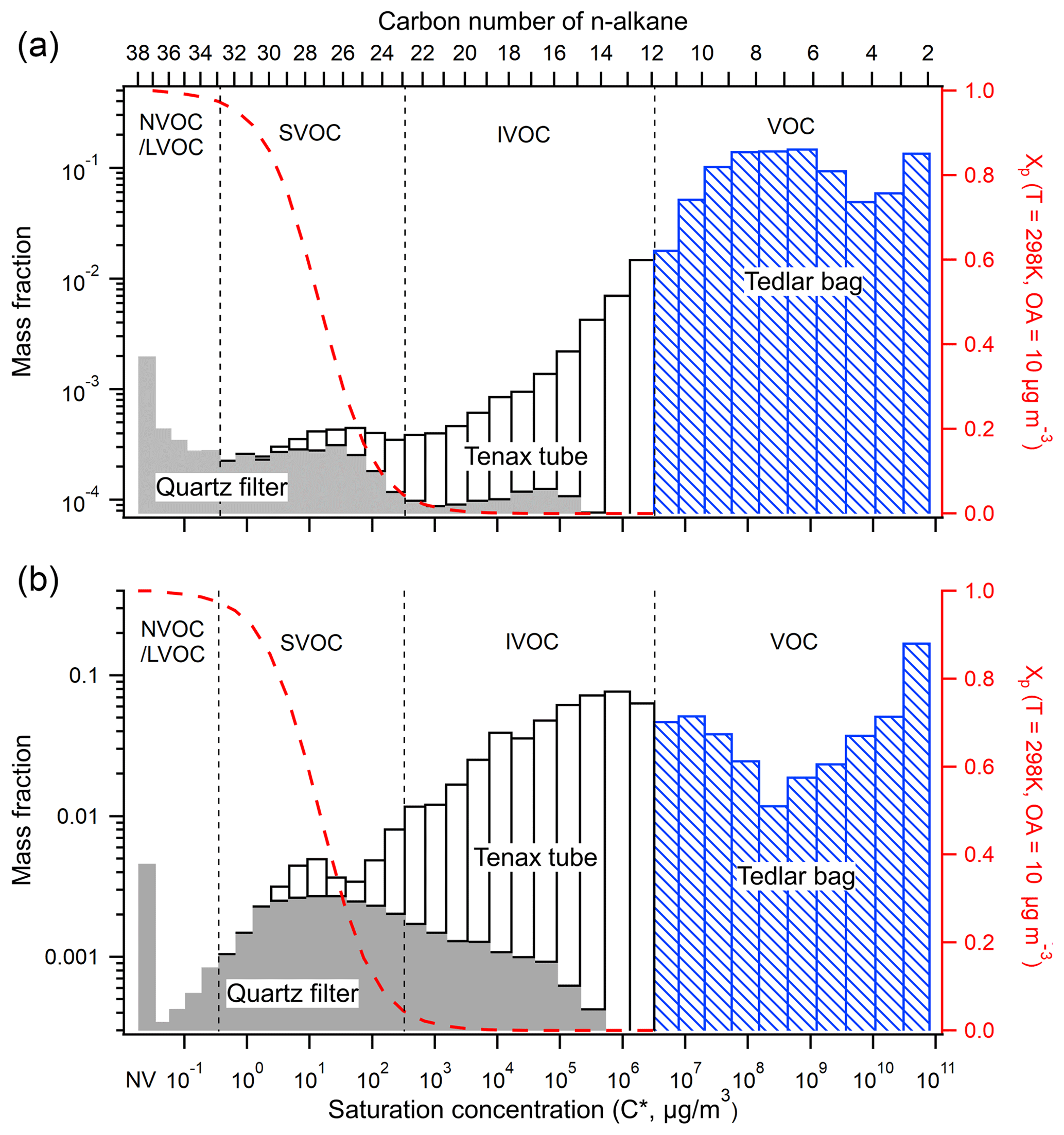
Figure 1Volatility distribution of organic emissions for a typical (a) gasoline (b) diesel vehicle. The emissions are classified by sampling media (line 1: Tedlar bag, line 2: bare quartz filter followed by two Tenax tubes). The red dashed line indicates the particle fraction assuming the emissions form a quasi-ideal solution at a COA of 10 µg m−3 and temperature of 298 K.
Figure 1 also shows the particle fraction (Xp) calculated assuming all organics form a quasi-ideal solution to illustrate gas-particle partitioning at typical atmospheric conditions (T=298 K, OA=10 µg m−3). At these conditions, IVOCs exist essentially exclusively in the gas phase, while SVOCs exist in both phases. To illustrate the changes in gas-particle partitioning of IVOCs and SVOCs across a wide range of atmospheric conditions, Fig. S5 shows the equilibrium particle fraction (Xp) for T between 273 and 320 K and OA concentration from 1 to 10 µg m−3. IVOCs are essentially exclusively in the gas phase (>99 %) except at very low temperature (T=273 K) and high OA loading (OA=10 µg m−3) conditions, when about 6 % of the lowest bin ( µg m−3) partitions to the particle phase. In contrast, SVOCs are always present in both gas and particle phases, in both hot and dilute (T=320 K and OA=1 µg m−3) or cold and high OA loading (T=273 K and OA=10 µg m−3) conditions.
Figure 1 indicates there is also substantial breakthrough of SVOCs from the quartz filter during mobile source certification testing (e.g. 2007 CFR 86), which requires maintaining a filter temperature of 47 ∘C. In our experiments, these SVOCs are collected by the downstream Tenax tubes. This breakthrough is denoted by the white bars in the SVOC range in Fig. 1; the SVOC breakthrough corresponds to, on average, 37 % of the total SVOC emissions from gasoline vehicles, 52 % for non-DPF diesel and 89 % for DPF diesel (Zhao et al., 2015, 2016). Therefore, quantitatively accounting for all gas-phase SVOCs requires using adsorbents. This is needed to improve predictions of POA concentrations and SOA production.
We compared the sum of NVOCs, LVOCs and SVOCs to the quartz-filter POA measurements. A linear regression of the on-road gasoline vehicle data yields a slope of 1.4 (Fig. S6a), which indicates that the quartz-filter-based POA emission factors should be multiplied by 1.4 to account for missing gas-phase SVOC emissions. This factor would be larger if the quartz filter did not collect some IVOC vapours as an adsorption artifact (Fig. 1). For off-road gasoline sources, a linear regression yields a slope of 1.1 (Fig. S6b), indicating a larger fraction of the SVOCs are collected on quartz filters compared to on-road gasoline vehicles. This is presumably due to shifts in gas-particle partitioning towards the particle phase at the high OA concentrations in the off-road source tests. For diesel sources, a linear regression yields a slope of 0.9 (Fig. S6c). This lower ratio is due to that filter-measured POA also including a positive adsorption artifact from IVOCs, which more than offsets the gas-phase SVOC breakthrough (Fig. 1b).
3.1 Emission factors
Figure 2a compares the total organics emission factors (NMOG +1.2 *OC) for on- and off-road gasoline vehicles, including LDGV, two-stroke small off-road engines (SORE-2S), and four-stroke small off-road engines (SORE-4S); gas-turbine engines; and on- and off-road diesel sources, including DPF-equipped engines. We subdivided the LDGV data based on emissions certification standard: pre-LEV (U.S. Tier0), LEV (California Low Emission Vehicle), and ULEV (California Ultra-Low Emission Vehicle).
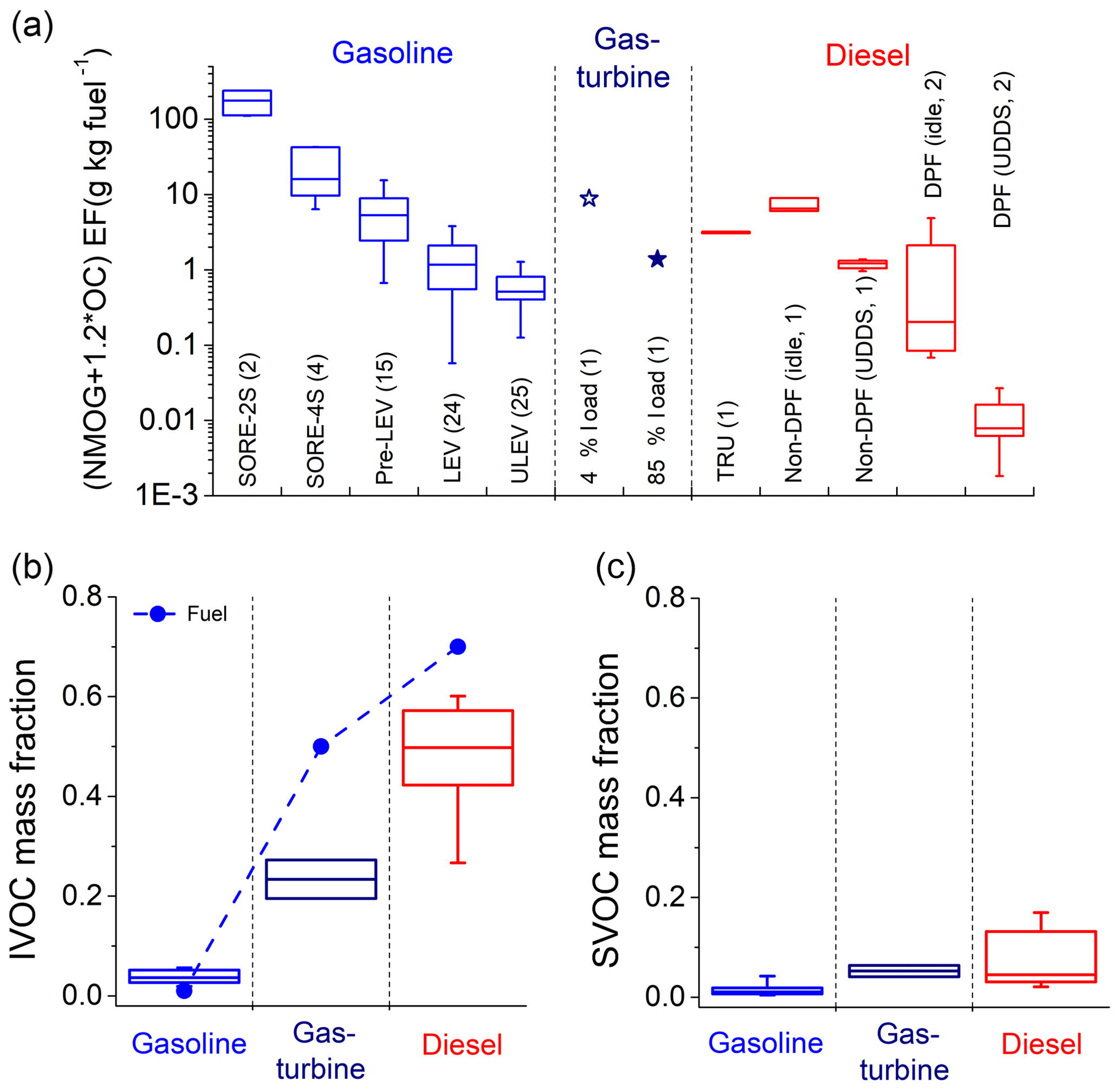
Figure 2(a) Emission factors for total organics (NMOG + 1.2 *OC) for different source categories. The number in parentheses indicates the number of unique sources tested in each category. Mass fraction of (b) IVOCs and (c) SVOCs in total organics for each source category. This figure only shows cold-start and off-road gasoline engine emissions. Box-whisker plot represents the range of emission for each category: 25th–75th percentiles and 10th–90th percentiles.
Although there is source-to-source variability within a given source category (e.g. pre-LEV gasoline or DPF-equipped diesel), there are distinct trends in total organic emissions. Gasoline small off-road engines (SORE) have the highest emissions, with SORE-2S having, on average, 1 order of magnitude higher emissions than SORE-4S (Gordon et al., 2013). This is due to less stringent regulations for off-road engine emissions (Cao et al., 2016a), and the unburned fuel mixing in exhaust due to the two-stoke design in SORE-2S. The LDGV emissions decrease with tightening emission standards (Gentner et al., 2017; May et al., 2014). For example, relative to the median Pre-LEV, there is a 78 % reduction in total organic emissions to the median LEV and 90 % to the median ULEV. Although not shown here, total organic emission factors are dramatically higher during cold-start than during hot-stabilized operations after the catalytic converter has reached its operating temperature (Saliba et al., 2017). Gas-turbine engine emissions show strong load dependence; idle (4 % thrust) emission is comparable to pre-LEV vehicles, and about an order of magnitude higher than high loads (85 % thrust) emission. Diesel emissions show strong dependence on both after-treatment devices and test cycle. DPF-equipped diesel vehicles have the lowest emission factors among all tested engine types. Lower emission factors are measured for high speed transient operations (e.g. UDDS cycle) compared to idle/low speed operations. The trends in gas-turbine and diesel emissions are qualitatively consistent with Cross et al. (2013, 2015) who showed similar load-dependent trend of decreasing THC or IVOC emission factors of gas-turbine and diesel engines with higher loads.
As expected, Fig. 2a indicates there is source-to-source variation in total organic emission for a given category (e.g. pre-LEV or ULEV). This variability reflects the effects of difference of engine design, engine calibration, after-treatment system, vehicle age, and maintenance history on emissions. However, the previously described trends in total organic emission among the different source categories are clear even with this variability.
3.2 Volatility and chemical composition distributions
Figure 3 shows the median volatility distributions of the emissions for three different source categories: gasoline (cold-start), gas-turbine and non-DPF diesel. For gas-turbine engine category, we plot the idle load (4 % thrust) emission.

Figure 3Median volatility distribution of organic emissions for (a) cold-start on-road gasoline, (b) gas-turbine (idle) and (c) on-road non-DPF diesel engines. The color shading indicates composition. Shaded area indicated by dashed indicate distribution for unburned fuel; dots indicate traditional source profiles from EPA SPECIATE database. The y axis has a broken scale to amplify the least volatile emissions.
Figure 3 indicates that the organic emissions from all three source categories have tri-modal volatility distributions. The dominant mode is the middle one, with a peak at µg m−3 for gasoline sources, µg m−3 for gas-turbine sources, and µg m−3 for diesel sources. For each source category, this mode has a similar volatility distribution and chemical composition as unburned fuel (Fig. S7). We therefore call it the “fuel mode”.
The fuel mode contributes 72.6 % (66.5 %–77.6 % as 10th to 90th percentile, same hereafter) of the total organic emissions in gasoline engine exhaust, 63.1 % (48.9 %–84.4 %) in diesel engine exhaust, and 37.5 %–38.5 % in gas-turbine source emissions. The widely varying contribution of this mode to diesel emissions is due, in part, to after-treatment and duty-cycle effects. For example, low-speed operation (creep and idle) test results show higher mass fractions in the fuel mode, 79.7 % (62.2 %–83.0 %), compared to high speed operations. The size of the fuel mode to DPF diesel vehicles is highly variable, 54.2 % (29.3 %–79.9 %), which is likely due in part to higher uncertainty associated with measuring very low emission rates.
Figure 3 highlights how the changes in fuel composition create systematic differences in volatility distribution of the emissions among the three source categories. Specifically, the “fuel” mode of the exhaust shifts towards lower volatility from gasoline to diesel sources mirroring the trend in fuel volatility. Although the chemical composition of the fuel mode is also similar to that of unburned fuel (Fig. S7), there are some important differences indicating that combustion and removal efficiencies vary by compound class, which are discussed in Sect. 3.4.
Emissions from each source have a low-volatility mode, comprised of SVOCs and even less-volatile organics. For all three source categories, this low-volatility mode peaks at µg m−3, which is in the middle of the SVOC range. Therefore, some of the organics in the low-volatility mode partition into the particle phase in the atmosphere to form POA, while the rest exist as vapours. The volatility distribution of this mode is similar to that of lubricating oil (May et al., 2013a, b; Worton et al., 2014); we therefore refer to the low-volatility mode as the “oil mode”. For diesel, the low-volatility and fuel modes blend together. The oil mode contributes 1.4 % (0.6 %–4.2 %) of the total organic emissions for gasoline sources, 4.2 %–12.1 % for the gas-turbine source, and 5.9 % (3.1 %–17.7 %) for diesel sources.
The size of the LDGV “oil mode” varies with certification standard, with median values of 0.8 % in Pre-LEV, 1.4 % in LEV and 2.2 % in ULEV. This trend indicates that improvements in after-treatment technology more effectively remove NMOG emission compared to POA emissions. The wide range of SVOC emissions from gas-turbine and diesel sources reflects the effects of changes in engine load/after-treatment: at 85 % engine load, 12.1 % of gas-turbine emissions are in the “oil mode” vs only 4.2 % at 4 % load. DPF-equipped vehicles show 14.8 % (10.1 %–30.6 %) of the emissions for on high-speed cycles vs a much lower fraction 2.1 % (1.7 %–5.7 %) at low-speed operations.
The third mode is the most volatile one, peaking at a or 1011 µg m−3. It contributes 25.9 % (21.1 %–31.0 %) of the total organics in gasoline emissions, 26.9 % (9.4 %–40.6 %) in diesel sources emissions, and 50.5 %–57.3 % in gas-turbine engine emissions. It is comprised of the smallest compounds, such as C2–C5 alkanes, alkenes and carbonyls, produced from the incomplete combustion and breakdown of fuel molecules (May et al., 2014). It also contains other compounds such benzene in the µg m−3. We therefore call it the “combustion by-product” mode. The composition of this mode varies modestly by source class.
The majority of the IVOC emissions are found in the lower volatility end of the fuel mode. For gasoline sources, IVOCs are in the lowest volatility tail of this mode. For the LDGV tested using cold-start unified cycle, IVOCs contribute 4.5 % (2.4 %–9.6 %) of the total organic emissions. This includes both heavily controlled and low emitting ULEV and less controlled and higher emitting pre-LEVs. IVOCs contribute a similar fraction to the organic emissions from largely uncontrolled and high emitting SOREs (Fig. 2). However, IVOCs contribute a larger fraction, 18.1 % (5.8 %–31.1 %) for organic emissions from LDGV operated over the hot-start unified cycle (Zhao et al., 2016). This suggests that catalytic converters may be less effective at removing lower volatility organics such as IVOCs, which is also consistent with the trends in SVOC data discussed above. However, only four vehicles were tested using the hot-start unified cycle and the IVOC faction varied widely. More research is needed to understand the effects of hot-operations and duty cycle in general on IVOC emissions.
For sources operating on less volatility fuel, IVOCs contribute a larger fraction of the emissions. For example, they contribute 20 %–27 % of gas-turbine engine emissions at idle and 85 % loads. This is somewhat larger than data from Cross et al. (2013), who reported that 10 %–20 % of NMHC emissions are IVOCs at idle load. The difference could be due to multiple factors, including differences in collection techniques (cryogenic vs adsorbent) and/or differences in fuel composition (Corporan et al., 2009). Diesel sources emit the highest fraction of IVOCs, with a median value of 51.3 % (28.7 %–61.5 %). Non-DPF-diesel emissions have a more consistent IVOC fraction of 57.1 % (46.3 %–66.4 %) than DPF-diesel emissions (40.1 %; 17.2 %–55.5 %). Finally, the contribution of IVOCs qualitatively mirrors the fuel composition: 1 % of unburned gasoline is comprised of IVOCs, ∼50 % for JP-8, and ∼70 % for diesel (Corporan et al., 2009; Gentner et al., 2012; May et al., 2014).
Figure 2c indicates that the contribution of SVOCs also differs by source type. For gasoline engines, SVOCs contribute 1.1 % (0.4 %–3.6 %) of the total organic emission. This variability is, in part, associated with the effects of tightening emissions certification standards as discussed above. For gas-turbines, SVOCs contribute 3.6 %–4.6 % of total organic emissions. For diesel source, SVOCs contribute 4.6 % (2.3 %–16.1 %) of the total organic emission; the wide range reflects effects of duty cycle and after-treatment as discussed above. There are no SVOCs in unburned gasoline and jet fuel, and less than 2 % for diesel fuel. The SVOCs in the emissions are likely predominantly from lubricating oil (Worton et al., 2014).
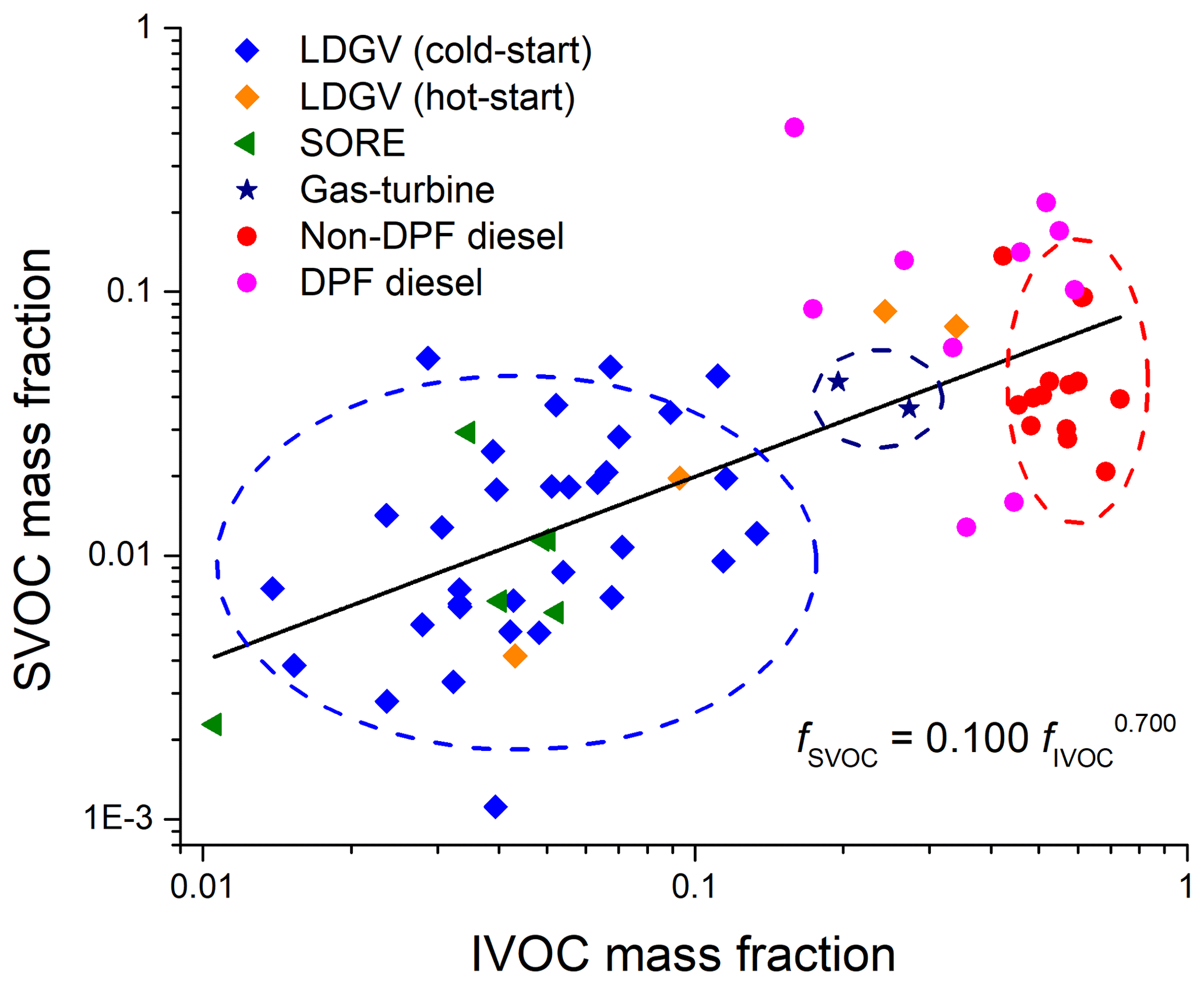
Figure 4Two-dimensional visualization of volatility distributions (x axis: IVOC mass fraction, y axis: SVOC mass fraction) of all tested sources. Dashed circles indicate clusters by fuel type. Blue cluster: gasoline (cold-start), navy: gas-turbine, red: non-DPF diesel source.
Given that the total organic emissions vary by more than 5 orders of magnitude (Fig. 2a), the volatility distribution (and emissions profiles) are relatively consistent across sources using the same fuel type (Fig. 3). As discussed previously, for a given fuel type, after-treatment technology (e.g. LDGV emission certification standard) and test cycle can also influence the volatility distribution, but their influence is much less than that of fuel. We therefore use the median distributions to represent the properties of the aggregate emissions from a large number of sources with a given source category. There is always source-to-source variability, but for inventories we need to define representative profiles for distinct categories (we use medians as opposed to averages to reduce the influence of outliers).
An important question is the number of distinct source categories. To investigate this question, Fig. 4 compares the volatility distributions of different sources in a two-dimensional space of IVOC vs SVOC mass fractions. These are important SOA precursors, so this framework highlights differences in SOA formation potential. There are three distinct clusters in Fig. 4, one for each fuel type (gasoline, diesel and jet). Therefore, these source categories require different profiles. For example, the on-road (cold-start) and off-road gasoline source emissions cluster, with median mass IVOC and SVOC fractions of 4.5 % and 1.1 %, respectively, indicating similar volatility distributions between on- and off-road gasoline sources. Figure 4 also suggests two additional categories, but these distinctions are not as strong given the variability of the data. First, hot-start LDGV emissions have much higher IVOC and SVOC fractions than cold-start emissions (18.1 % vs 4.5 %, 4.7 % vs 1.1 %). This implies a roughly 4 times higher SOA yield for hot-start on-road gasoline emissions. Therefore, separate profiles should be used to represent cold-start and hot-operation emissions when constructing emission inventories for gasoline vehicles. Second, DPF and non-DPF-equipped diesel sources also show significant different volatility distributions, especially in SVOC mass fraction (12.2 % vs 3.8 %). To account for these differences, we present five emission profiles in Table S3: gasoline (cold-start and off-road), gasoline (hot-start), diesel (non-DPF), diesel (DPF) and gas-turbine engines. Interestingly, the SVOC and IVOC mass fractions are strongly positive-correlated across all sources, with an exponential fit between SVOC and IVOC mass fraction of . One could certainly define additional source categories to, for example, account for trends in SVOC fraction with emission certification of LDGVs, but it is not clear that those difference are large enough to improve model performance vs using an aggregate profile to represent all gasoline vehicles.
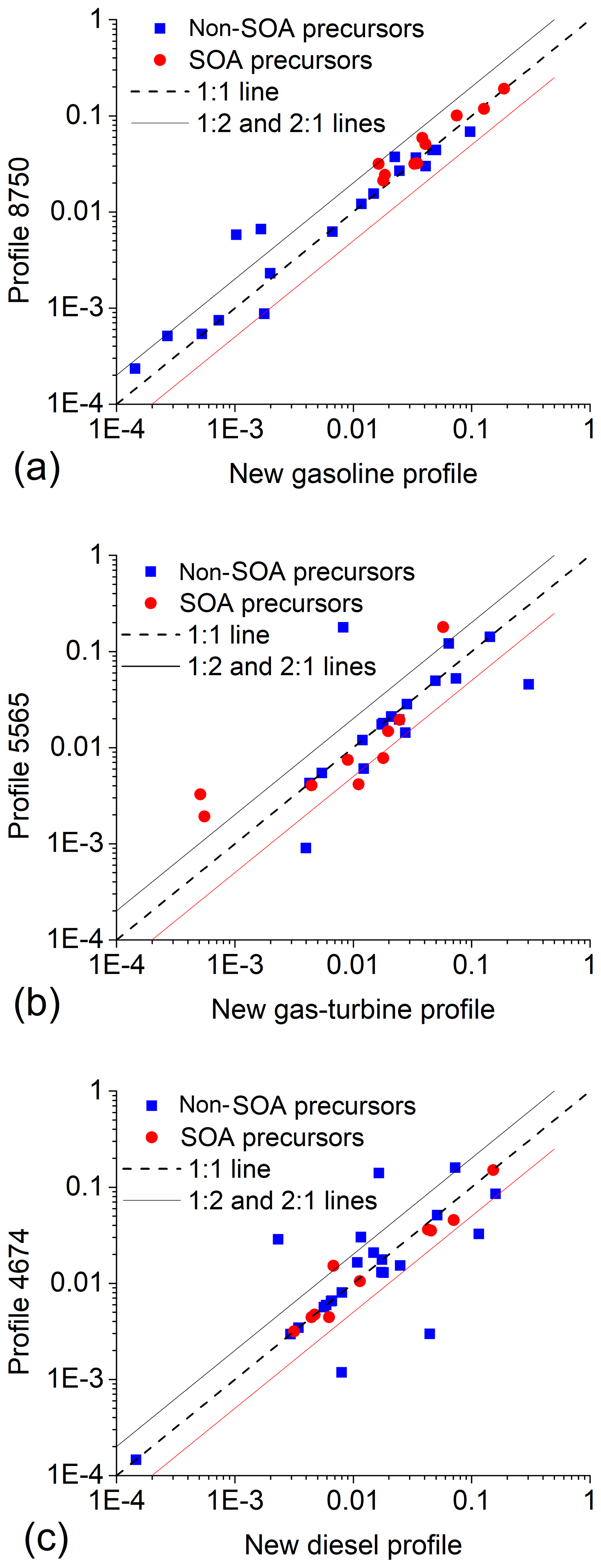
Figure 5Scatter plot of VOC groups in the SAPRC mechanism in the new profiles and in the SPECIATE database for (a) on-road gasoline, and cold-start (b) gas-turbine and (c) non-DPF diesel sources, demonstrating consistency between traditional and new profiles in VOC speciation.
3.3 New vs traditional source profiles
Figure 3 also compares our new comprehensive source profiles to traditional profiles used to construct the emission inventory to simulate air quality in the Los Angeles region during the 2010 CALNEX campaign (Baker et al., 2015). Our new profiles are the median value of the measured emission for gasoline (separate for cold-start and hot-operations), gas turbine, non-DPF and DPF-diesel sources; they are listed in Table S3 (Supporting Information). The traditional profiles are from the EPA SPECIATE database (USEPA, 2016b) – profile #4674 for diesel, #8750a for gasoline, and #5565 for gas turbine sources with the POA fraction (NVOC) calculated using MOVES (USEPA, 2014).
There is good agreement between our new and traditional profiles in the VOC range, with both having similar chemical compositions and volatility distributions containing both by-product and fuel modes (Fig. 3). For example, Fig. 5 demonstrates the strong agreement for SARPC-lumped VOC groups between the new and traditional profiles for all three source categories, with more than 90 % of the SAPRC groups for the gasoline sources agreeing within a factor of 2. We recommend using our new profiles for VOC composition because they have enhanced VOC speciation from combining the existing SPECIATE profiles with our new experimental data.
However, the traditional profiles dramatically underestimate IVOCs and SVOCs, which are important classes of SOA precursors. As illustrated in Fig. 1, this is a consequence of the limitations of traditional source characterization techniques to quantitatively collect and analyse IVOCs. For example, the traditional LDGV emission profile only attributes 0.2 % of the total organics to IVOCs vs 4.6 % in our new cold-start profile. The traditional gas-turbine engine emission profile attributes 13 % of the organics to IVOCs vs 27 % IVOCs in our new profile. For diesel vehicle emissions, the traditional profile attributes 10 % of total organic emission to IVOCs vs 54.2 % of organics for non-DPF diesel in our new profile. The traditional diesel source profile does contain about 20 % unknown organics (UNK), part of which are likely IVOCs, as the collection and chemical analysis efficiency decrease towards lower-volatility bins such as 103 and 104 µg m−3 (Fig. 3). However, most UNK are not represented as IVOCs in models, as discussed in Sect. 2.2.
3.4 Exhaust vs unburned fuel and IVOC enrichment factors
Figure 3 highlights the large contribution of unburned fuel to the exhaust, but careful examination of the data reveals that the combustion process and/or removal efficiency by the after-treatment device are compound dependent. For example, gasoline and gas-turbine emission are both enriched in IVOCs compared to fuel (e.g. µg m−3 for gasoline, and µg m−3 for gas-turbine). The difference suggests higher combustion efficiency of more volatile fuel components.
Figure S8 compares the chemical composition of the exhaust to unburned fuel. Overall, straight and branched alkanes (speciated and unspeciated) contribute a smaller fraction to the exhaust than in the fuel, with the median mass fractions decreasing from 46.6 % (fuel) to 34.3 % (exhaust) for gasoline sources, 50.0 % to 9.8 % for gas-turbine sources, and 30.3 % to 11.2 % for diesel sources. In comparison the fractions of aromatic and cyclic compounds (speciated and unspeciated) are consistent between fuel and exhaust: for example, 37.2 % (exhaust) vs 36.1 % (exhaust) for gasoline sources and 58.7 % to 60.2 % for diesel sources. This comparison implies higher combustion efficiencies of n-/b-alkanes than cyclic/aromatic compounds in internal combustion engines, which could partly be explained by the flash points of different hydrocarbons. The mass fraction of alkenes, alkynes and carbonyls increase, indicating they are important products of incomplete combustion. For example, they increase from 3.5 % (fuel) to 28.6 % (exhaust) for gasoline sources, and from 0 % to 54.5 % and 24 % for gas-turbine and diesel sources, respectively. Gasoline emissions have the highest single-ring aromatics fraction (∼30 %), compared to 5.5 % in gas-turbine and 17 % in diesel emissions. This mirrors fuel composition – unburned gasoline fuel had the highest aromatic content (26.7 %) of the fuels tested here.
We are especially interested in the enrichment or depletion of SOA precursors in the exhaust compared to fuel, including IVOCs and single-ring aromatics. To quantify enrichment, we normalized SOA precursors in both the fuel and exhaust to C8 to C10 n-alkanes, a tracer for the unburned fuel. As shown in Figs. S7 and S9, some SOA precursors are enriched, and others depleted relative to fuel. Benzene and total IVOCs in gasoline and toluene and C8 aromatics in diesel exhaust are enriched by more than a factor of 2 relative to unburned fuel. Enrichment of single-ring aromatics are likely due to pyrolysis of larger aromatic molecules (Akihama et al., 2002; Brezinsky, 1986). In contrast, total IVOCs (normalized to the C8 to C10 n-alkanes) are depleted in diesel exhaust compared to fuel (enrichment factors less than 1).
Figure 6 shows box-whisker plots of the total IVOC enrichment factors. Sources using more volatile fuel have higher IVOC enrichment factors. For example, relative to C8–10 n-alkanes, gasoline engine exhaust has a median total IVOC enrichment factor of 8.5 vs modest depletion (enrichment factor <1) in diesel source exhaust, with gas turbine exhaust in between. There are several possible explanations for this trend. IVOCs may be less efficiently combusted in the engines. Recent research also shows that fewer IVOCs are removed by catalytic converters compared to VOCs (Pereira et al., 2018). Figure S10 plots the IVOC enrichment factors of Pre-LEV, LEV and ULEV vehicle exhaust. Due to the different removal efficiency between IVOCs and VOCs, median ULEV vehicles show an even higher (>10) IVOC enrichment factor. Lubricating oil decomposition products may also contribute to the IVOC emissions (May et al., 2013a; Worton et al., 2014). Finally, the IVOC fraction in fuel may be underestimated due to limitations in techniques used commonly to characterize fuel composition (Gentner et al., 2012).

Figure 6IVOC mass enrichment factors as a function of IVOC content in fuel, . The box-whisker plots indicate variability in ratio within a given source class: 25th–75th percentiles and 10th–90th percentiles.
Table 1List of different estimates of IVOC emissions and SOA yield for mobile sources shown in Fig. 7.
aFrom Koo et al. (2014).
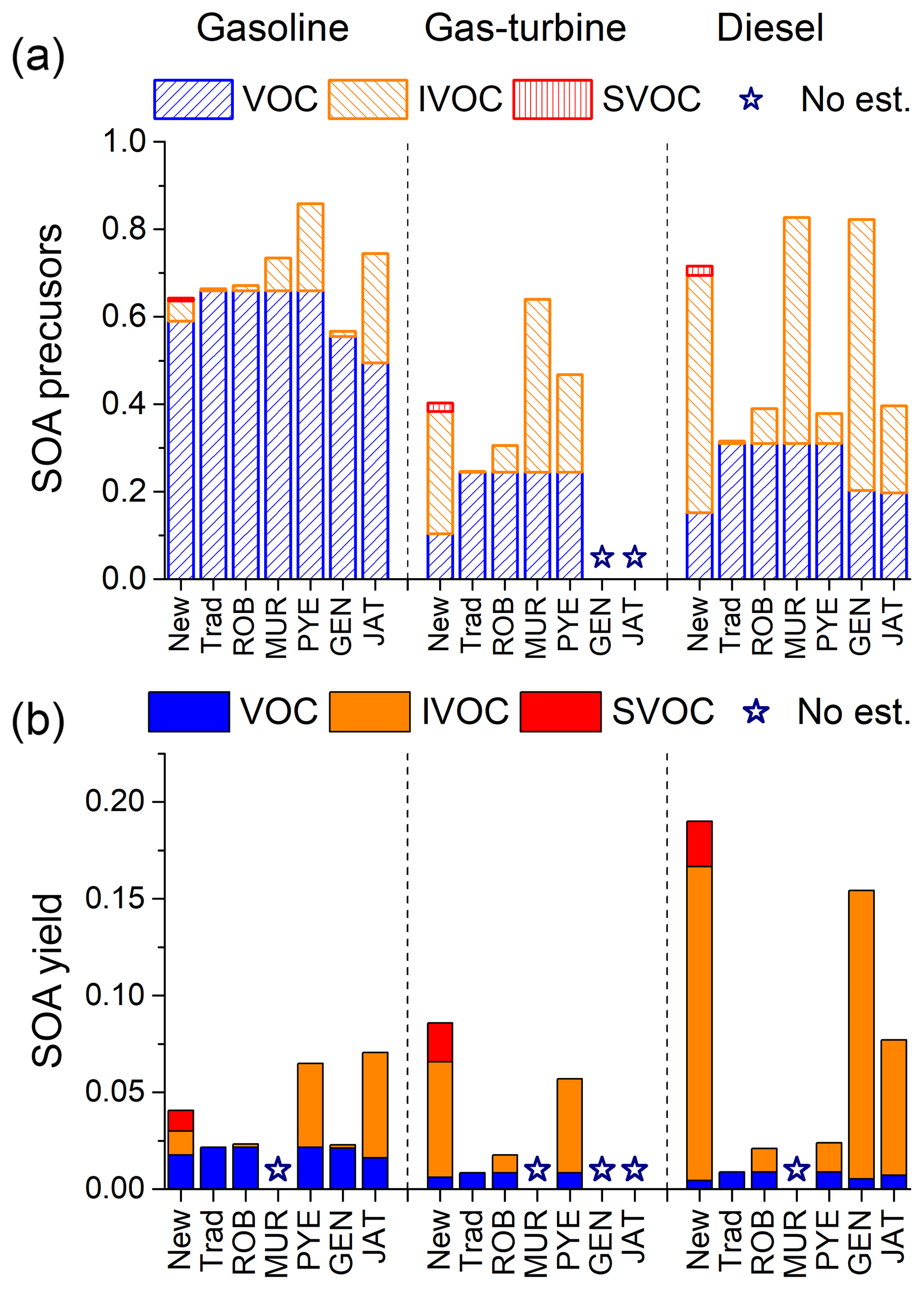
Figure 7Comparison of (a) mass fraction of SOA precursors in total NMOG emissions and (b) calculated total SOA yields of NMOG emissions from mobile sources based on the different estimation approaches listed in Table 1. Star denotes no estimate available.
An important goal of this work is to develop emission profiles required to improve model predictions of SOA formation. Simulation of ambient OA concentrations requires accurate representation of both emissions and SOA yields for SVOCs and IVOCs. Given the lack of IVOC data in traditional source profiles (Fig. 3), previous modelling studies have used different scaling approaches, most commonly based on POA (Koo et al., 2014; Murphy et al., 2017; Robinson et al., 2007; Woody et al., 2016) but also using NMOG (Jathar et al., 2014, 2017) and naphthalene (Pye and Seinfeld, 2010). Finally, Gentner et al. (2012) used unburned fuel surrogate to estimate IVOC emissions. These estimates are then combined with SOA yield data.
In this section, we use our new data to evaluate these different scaling approaches for estimating IVOC emissions to better understand their strengths and limitations for simulating ambient OA concentrations. Table 1 lists the different approaches we evaluated: (1) New – new profiles developed in this paper; (2) Trad – traditional profiles (SPECIATE no. 8750a for gasoline, no. 5565 for gas-turbine and no. 4674 for diesel source emissions); (3) ROB: traditional profiles POA as IVOCs (Robinson et al., 2007); (4) MUR: traditional profiles POA as IVOCs (Murphy et al., 2017); (5) PYE: traditional profiles naphthalene as IVOCs (Pye and Seinfeld, 2010); (6) GEN: using unburned fuel composition as surrogate (Gentner et al., 2012); (7) JAT: 20 % of NMOG of gasoline emission and 25 % of diesel emissions are IVOCs (Jathar et al., 2014).
Figure 7 compares our new data to the six previous estimates. Figure 7a shows the mass fraction of different classes of SOA precursors (VOC, IVOC and SVOC) in the NMOG emissions. Figure 7b shows the overall SOA yields of the total NMOG emissions for the different models (SOA mass/mass of NMOG emissions).
As shown in Fig. 7a, all estimates have similar VOC SOA precursor mass fractions, but widely divergent amounts of IVOCs. Our new profiles (1) and estimates (6) and (7) have modestly lower VOC SOA precursors, due to the inclusion of IVOCs and gas-phase SVOC within NMOG emissions, while approaches (3)–(5) add additional IVOCs to the existing NMOG emissions. Since FID-based NMOG is a measure of all non-methane organic gases, we think IVOCs and gas-phase SVOCs are largely accounted for in existing NMOG emission factors for the types of sources measured here (see discussion of mass closure between bulk measurements and speciated measurements in Sect. 2.2 and Fig. S3). However, traditional source profiles do not correctly attribute these emissions to IVOCs ∕ SVOCs in all sources.
The most common approach to incorporate IVOCs in models has been to scale POA emissions as defined by the organic mass collected on a quartz filter. The scaling ratios (e.g. IVOC-to-POA) were estimated from very limited data (a single or small number of sources) and the same ratio has typically been applied to all source categories. Our data indicate that scaling with POA is not a robust approach because IVOC-to-POA ratios vary by source category. For example, the average IVOC-to-POA ratios for gasoline engine exhaust are 6.2±4.4 (cold-start) vs 12±7 (non-DPF-equipped) and 31 (DPF-equipped) for diesel exhaust (Zhao et al., 2015, 2016). In addition, these values are much larger than the widely used scaling factor of IVOC-to-POA of 1.5 (ROB in Fig. 7) (Robinson et al., 2007), which grossly underestimates the IVOC emissions from the types of internal combustion engines considered here, while the IVOC-to-POA ratio of 9.6 by Murphy et al. (2017) (MUR in Fig. 7) overestimates IVOC emissions from gasoline and gas-turbine sources, but underestimates it from diesel sources.
However, even if one uses source-specific IVOC-to-POA scaling factors, we do not think that scaling POA provides a robust estimate of IVOC emissions from internal combustion engines. POA emissions are dominated by lubricant oil (Worton et al., 2014), while IVOC emissions appear to mainly arise from unburned fuel (Fig. 2). In addition, quartz filter measurements are subject to sampling artifacts and partitioning biases (May et al., 2013a, b, c). As a result, IVOC-to-POA ratios vary not only by source type (e.g. gasoline vs diesel), but also by operating conditions (Zhao et al., 2015).
Zhao et al. (2015, 2016) reported stronger correlations between IVOC and total NMOG emissions than with POA over a range of operating conditions (R2=0.96 vs 0.90 for gasoline and R2=0.99 vs 0.91 for diesel sources, Fig. S11). This is not surprising given that both NMOG and IVOC emissions arise from fuel and are controlled by similar processes. This suggests that IVOC emissions should be estimated using source-specific scaling factors of NMOG, not POA.
Jathar et al. (2014, 2017) estimated IVOC emissions by scaling NMOG. They also used different ratios for gasoline and diesel sources. However, they did not directly measure IVOCs. Instead they inferred IVOC-to-NMOG ratios using a combination of unspeciated emissions and inverse modelling of SOA production measured in a smog chamber. Using this approach, they attributed 25 % of NMOG emission from gasoline engine and 20 % from diesel engines to IVOCs. These values are very different than those reported here, which are based on direct measurements. A detail on the ratios of Jathar et al. (2014) is that they were derived to be used in combination with their empirically derived SOA yields. When used together they explain SOA yield production measured in smog chamber experiments with dilute exhaust. Therefore, one cannot simply replace IVOC-to-NMOG of Jathar et al. (2014) with the ones reported here without also using different SOA yields.
Pye and Seinfeld (2010) estimated IVOC emissions by scaling naphthalene using the same IVOC-to-naphthalene ratio for all sources. Our data indicate that naphthalene is not a good indicator of IVOCs, due to the large variation in fuel aromatic content. For example, there is four times more naphthalene in gasoline engine exhaust (0.4 %) and fuel (0.13 %) compared to diesel engine exhaust (0.1 %) and fuel (0.04 %). Therefore, the approach of Pye and Seinfeld (2010) generates much higher estimates of IVOC emissions from gasoline than diesel sources, which is opposite of the actual emissions data (Fig. 2). In principle, this problem can be overcome with source specific IVOC-to-naphthalene ratios, but even with source-specific ratios, individual organics are likely a less robust scaler for IVOCs than total NMOG because fuel composition (e.g. aromatic content) varies by location and season.
A final approach to estimate IVOC emissions is to use unburned fuel as a surrogate for the SOA production of exhaust. Gentner et al. (2012) used this approach to estimate the IVOC fraction, as well as the SOA yield of gasoline and diesel engine exhaust. This approach works for diesel, but not for gasoline given the enrichment of IVOCs in the exhaust (Fig. 6).
In Fig. 7b, we combine the different emissions estimates with SOA yield data to calculate the SOA yield of the NMOG emissions for each source category, assuming complete oxidation of all precursors. Our new profiles predict that IVOCs and SVOC vapours contribute substantially to SOA production, especially for sources using lower-volatility fuels (e.g. diesel). For gasoline sources, we predict that IVOCs and SVOCs contribute as much SOA as traditional VOC precursors (mainly single-ring aromatics). Accounting for IVOCs in gasoline exhaust almost doubles the predicted SOA production compared to the traditional profile. For gas-turbine and diesel sources, IVOCs and SVOC vapours combined contribute factors of 13 and 44 more SOA than VOCs, respectively.
Figure 7b also compares the SOA yields of NMOG emissions for all the different approaches (2)–(7). The differences in effective yields are primarily due to differences in IVOC ∕ SVOC emissions. Traditional profiles and ROB underpredicts SOA production from all three source categories because they underestimate IVOC emissions. As discussed in Sect. 3.4, IVOCs are enriched in gasoline emissions compared to unburned fuel; therefore, GEN underpredicts the SOA yield of gasoline emissions. However, fuel composition provides a reasonable estimate for SOA production from diesel emissions, except for the lack of SVOCs potentially produced from the usage of lubricant oil. The approaches of PYE and JAT overpredict the overall SOA production from gasoline emissions, due to their overestimation of IVOC emissions, but both underestimate the overall SOA production for diesel emissions.
To conclude, none of the previous modelling approaches provide a robust estimate of the IVOC fraction in the exhaust for all three source categories. Figure 7 shows that traditional profiles either completely omit IVOCs or incorrectly lumped them to VOC chemical mechanism groups, which greatly underestimate the overall SOA formation potential. Approaches (3)–(5) apply scaling factors to certain species, such as POA and naphthalene, but these factors vary by source and fuel composition, which may lead to significant bias for different sources. Using unburned fuel composition as a surrogate in estimation (6) only works for sources that use lower volatility fuel, such as diesel.
In addition to better representing gas-phase SOA precursor emissions, the new profiles also account for the semi-volatile character of POA. Partitioning calculations predict that 40 % to 50 % of traditionally defined POA mass evaporates at typical atmospheric conditions (T=298 K and OA=10 µg m) (May et al., 2013a, b).
Figure 7 highlights the importance of including IVOC and SVOC emissions in models and inventories to improve predictions of SOA formation. This paper facilitates this by providing model-ready profiles that include direct measurements of IVOCs and SVOCs. They are designed to be applied to existing inventories of POA and NMOG emissions. These profiles (Table S3) are normalized to total organic emissions (VOC, IVOC, SVOC, LVOC plus NVOC), and therefore should be applied to the sum of gas- and particle-phase organic emissions. Since current emission inventories report gas- (NMOG or VOC) and particle-phase (PM or POA) emissions separately, the comprehensive profile can be separated into two parts: gas-phase (VOC and IVOC) and particle-phase (SVOC and less volatile components) profiles. These sub-profiles would be renormalized and then applied to the existing NMOG or POA emissions. With this approach, one needs to correct the POA data for missing SVOC vapours not collected during vehicle certification testing (the factor of 1.4 for LDGV discussed at the beginning of Sect. 3).
Our new profiles intentionally do not define the phase state of the emissions. Phase state is not a property of the emissions, but determined by the combination of the volatility distribution of the emissions and atmospheric conditions because gas-particle partitioning depends on the concentration of organic aerosol and temperature. The profiles specify the volatility distribution of the emissions, which can then be used to calculate the gas-particle partitioning (phase state) for any atmospheric condition (Robinson et al., 2010). This approach is critical to correctly predict POA concentrations for sources that have substantial SVOC emissions, such as the sources tested here and biomass smoke (May et al., 2013c).
The three types of sources considered here account for 98.2 % of the mobile source emissions in the 2014 US EPA National Emission Inventory. For other liquid-fuel internal combustion engine sources, we recommend interpolating based on fuel composition and applying the IVOC enrichment factor estimated from fuel volatility (Fig. 6). For sources profiles that only contain speciated VOCs and unknown residual, we recommend not normalizing to known species, as this will likely misattribute low-volatility organics to VOCs.
The emission profiles described here (except for gas turbines) are based on experiments conducted using sources recruited from the California in-use fleet, at typical California summertime temperatures (10–25 ∘C) and using California commercial summertime fuels. Therefore, the data are most directly relevant to California summertime conditions. Ambient temperature can have a large influence on emissions. For example, George et al. (2015) measured about 10 times higher non-methane hydrocarbon (NMHC) emission rates during testing at −7 ∘C vs 24 ∘C. The VOC composition also changed with temperature, with the fraction of C9+ aromatics almost doubling at low temperature. These data suggest that winter emissions may have a higher content of larger aromatics (C9+ aromatics) and IVOCs, due to incomplete combustion or lower efficiency of catalytic converter. Our profiles therefore likely represent lower bounds to winter vehicle emission in terms of aromatics and IVOC contents. As discussed in Sect. 3.2, unburned fuel is an important contributor to the emissions. Therefore, variations in fuel composition by, for example, season and/or location will influence the composition of the emissions. From an SOA formation perspective, we are most interested in changes in fuel IVOC and aromatic content. Figure S12 compares our new VOC profiles with data from China (Cao et al., 2016b; Yao et al., 2015). There is good agreement for many compounds, but not all.
Future research needs the following.
-
IVOC and SVOC emissions data from vehicles operated over a wider range of conditions. Comprehensive emissions data are needed for a wider range of fuel compositions, test cycles (hot operations), and seasons (especially winter). However, given their major contribution to SOA formation, we recommend using our new profiles even for studies outside of California if the only other option is to use traditional profiles that don't include IVOC and SVOC data.
-
IVOC and SVOC emissions data for non-mobile sources. Recent research has demonstrated that IVOCs and SVOCs are important contributors to biomass burning, oil sands, oil production, and volatile chemical product emissions (de Gouw et al., 2011; Hatch et al., 2017; Hunter et al., 2017; Liggio et al., 2016). More comprehensive, model-ready profiles that account for the full spectrum of organic emissions are needed for these and other source categories (McDonald et al., 2018).
-
Inclusion of IVOCs in air quality models and inventories. Our new profiles are designed to directly incorporate IVOCs into models and inventory. Since they are based on direct measurements, they do not have the large uncertainties associated with the previously developed scaling approaches.
-
Improved chemical composition of IVOCs and SVOCs. Although we have quantified the total IVOC emissions, the majority of these emissions were not resolved at the molecular level. Since the SOA yield of compounds depend on both molecular structure and volatility (Tkacik et al., 2012; Ziemann, 2011), future studies are needed to more fully speciate IVOCs and SVOCs in order to identify the class of compounds that needed for photo-oxidation experiments (Chan et al., 2013; Cross et al., 2015; Isaacman et al., 2012b).
-
Measurements and source apportionment of atmospheric IVOCs ∕ SVOCs. Ambient measurements of IVOCs ∕ SVOCs are needed to identify other important sources of atmospheric IVOCs ∕ SVOCs. This will help future studies to prioritize which sources to characterize.
Measurement data for on-road vehicles are documented in May et al. (2014). Measurement data for off-road engines are documented in Gordon et al. (2013). Measurement data for gas-turbine engine are available in Presto et al. (2011). Measurement data for IVOCs and SVOCs are available in Zhao et al. (2015, 2016). Normalized volatility distributions derived in this work can be found in Table S7 in the Supplement.
The supplement related to this article is available online at: https://doi.org/10.5194/acp-18-17637-2018-supplement.
QL, YZ and ALR designed the research. QL and YZ analysed the data. QL, YZ and ALR wrote the paper.
The authors declare that they have no conflict of interest.
This publication was developed as part of the Center for Air, Climate, and
Energy Solutions (CACES), which is supported under Assistance Agreement No.
RD83587301 awarded by the U.S. Environmental Protection Agency. It has not
been formally reviewed by EPA. The views expressed in this document are
solely those of authors and do not necessarily reflect those of the Agency.
EPA does not endorse any products or commercial services mentioned in this
publication. The authors would like to thank Albert Presto, Timothy Gordon
and Andrew May for their help in providing detailed datasets information. The
authors would also like to thank Benjamin Murphy and Havala Pye for helpful
comments on this manuscript and valuable discussion on missing SVOC scaling
approach.
Edited by: Qiang
Zhang
Reviewed by: two anonymous referees
Adelman, Z., Vukovich, J., and Carter, W.: Integration of the SAPRC Chemical Mechanism in the SMOKE Emissions Processor for the CMAQ/Models – 3 Airshed Model, available at: https://escholarship.org/uc/item/928332x8 (last access: 12 July 2018), 2005.
Akihama, K., Takatori, Y., and Nakakita, K.: Effect of hydrocarbon molecular structure on diesel exhaust emissions, Toyota Central R&D Labs., Inc., Nagakute, Japan, 37, 46–52, 2002.
Baker, K. R., Carlton, A. G., Kleindienst, T. E., Offenberg, J. H., Beaver, M. R., Gentner, D. R., Goldstein, A. H., Hayes, P. L., Jimenez, J. L., Gilman, J. B., de Gouw, J. A., Woody, M. C., Pye, H. O. T., Kelly, J. T., Lewandowski, M., Jaoui, M., Stevens, P. S., Brune, W. H., Lin, Y.-H., Rubitschun, C. L., and Surratt, J. D.: Gas and aerosol carbon in California: comparison of measurements and model predictions in Pasadena and Bakersfield, Atmos. Chem. Phys., 15, 5243–5258, https://doi.org/10.5194/acp-15-5243-2015, 2015.
Brezinsky, K.: The high-temperature oxidation of aromatic hydrocarbons, Prog. Energy Combust. Sci., 12, 1–24, https://doi.org/10.1016/0360-1285(86)90011-0, 1986.
Cao, T., Durbin, T. D., Russell, R. L., Cocker, D. R., Scora, G., Maldonado, H., and Johnson, K. C.: Evaluations of in-use emission factors from off-road construction equipment, Atmos. Environ., 147, 234–245, https://doi.org/10.1016/j.atmosenv.2016.09.042, 2016a.
Cao, X., Yao, Z., Shen, X., Ye, Y., and Jiang, X.: On-road emission characteristics of VOCs from light-duty gasoline vehicles in Beijing, China, Atmos. Environ., 124, 146–155, https://doi.org/10.1016/j.atmosenv.2015.06.019, 2016.
Carter, W. P. L.: Development of the SAPRC-07 chemical mechanism, Atmos. Environ., 44, 5324–5335, https://doi.org/10.1016/j.atmosenv.2010.01.026. 2010.
Carter, W. P. L. L.: Development of a database for chemical mechanism assignments for volatile organic emissions, J. Air Waste Manage. Assoc., 65, 1171–1184, https://doi.org/10.1080/10962247.2015.1013646, 2015.
Chan, A. W. H., Kautzman, K. E., Chhabra, P. S., Surratt, J. D., Chan, M. N., Crounse, J. D., Kürten, A., Wennberg, P. O., Flagan, R. C., and Seinfeld, J. H.: Secondary organic aerosol formation from photooxidation of naphthalene and alkylnaphthalenes: implications for oxidation of intermediate volatility organic compounds (IVOCs), Atmos. Chem. Phys., 9, 3049–3060, https://doi.org/10.5194/acp-9-3049-2009, 2009.
Chan, A. W. H., Isaacman, G., Wilson, K. R., Worton, D. R., Ruehl, C. R., Nah, T., Gentner, D. R., Dallmann, T. R., Kirchstetter, T. W., Harley, R. A., Gilman, J. B., Kuster, W. C., De Gouw, J. A., Offenberg, J. H., Kleindienst, T. E., Lin, Y. H., Rubitschun, C. L., Surratt, J. D., Hayes, P. L., Jimenez, J. L., and Goldstein, A. H.: Detailed chemical characterization of unresolved complex mixtures in atmospheric organics: Insights into emission sources, atmospheric processing, and secondary organic aerosol formation, J. Geophys. Res.-Atmos., 118, 6783–6796, https://doi.org/10.1002/jgrd.50533, 2013.
Corporan, E., Edwards, T., Shafer, L., DeWitt, M. J., Klingshirn, C., Zabarnick, S., West, Z., Striebich, R., Graham, J., and Klein, J.: Chemical, thermal stability, seal swell and emissions characteristics of jet fuels from alternative sources, 11th Int. Conf. Stability, Handl. Use Liq. Fuels, 2, 973–1014, 2009.
Cross, E. S., Hunter, J. F., Carrasquillo, A. J., Franklin, J. P., Herndon, S. C., Jayne, J. T., Worsnop, D. R., Miake-Lye, R. C., and Kroll, J. H.: Online measurements of the emissions of intermediate-volatility and semi-volatile organic compounds from aircraft, Atmos. Chem. Phys., 13, 7845–7858, https://doi.org/10.5194/acp-13-7845-2013, 2013.
Cross, E. S., Sappok, A. G., Wong, V. W., and Kroll, J. H.: Load-Dependent Emission Factors and Chemical Characteristics of IVOCs from a Medium-Duty Diesel Engine, Environ. Sci. Technol., 49, 13483–13491, https://doi.org/10.1021/acs.est.5b03954, 2015.
Di, Q., Wang, Y., Zanobetti, A., Wang, Y., Koutrakis, P., Choirat, C., Dominici, F., and Schwartz, J. D.: Air Pollution and Mortality in the Medicare Population, N. Engl. J. Med., 376, 2513–2522, https://doi.org/10.1056/NEJMoa1702747, 2017.
Donahue, N. M., Robinson, A. L., Stanier, C. O., and Pandis, S. N.: Coupled Partitioning, Dilution, and Chemical Aging of Semivolatile Organics, Environ. Sci. Technol., 40, 2635–2643, https://doi.org/10.1021/es052297c, 2006.
Drozd, G. T., Miracolo, M. A., Presto, A. A., Lipsky, E. M., Riemer, D. D., Corporan, E., and Robinson, A. L.: Particulate Matter and Organic Vapor Emissions from a Helicopter Engine Operating on Petroleum and Fischer–Tropsch Fuels, Energ. Fuel., 26, 4756–4766, https://doi.org/10.1021/ef300651t, 2012.
Ensberg, J. J., Hayes, P. L., Jimenez, J. L., Gilman, J. B., Kuster, W. C., de Gouw, J. A., Holloway, J. S., Gordon, T. D., Jathar, S., Robinson, A. L., and Seinfeld, J. H.: Emission factor ratios, SOA mass yields, and the impact of vehicular emissions on SOA formation, Atmos. Chem. Phys., 14, 2383–2397, https://doi.org/10.5194/acp-14-2383-2014, 2014.
Fujitani, Y., Saitoh, K., Fushimi, A., Takahashi, K., Hasegawa, S., Tanabe, K., Kobayashi, S., Furuyama, A., Hirano, S., and Takami, A.: Effect of isothermal dilution on emission factors of organic carbon and n-alkanes in the particle and gas phases of diesel exhaust, Atmos. Environ., 59, 389–397, https://doi.org/10.1016/j.atmosenv.2012.06.010, 2012.
Gabele, P.: Exhaust Emissions from Four-Stroke Lawn Mower Engines, J. Air Waste Manage. Assoc., 47, 945–952, https://doi.org/10.1080/10473289.1997.10463951, 1997.
Gentner, D. R., Isaacman, G., Worton, D. R., Chan, A. W. H., Dallmann, T. R., Davis, L., Liu, S., Day, D. A., Russell, L. M., Wilson, K. R., Weber, R., Guha, A., Harley, R. A., and Goldstein, A. H.: Elucidating secondary organic aerosol from diesel and gasoline vehicles through detailed characterization of organic carbon emissions, P. Natl. Acad. Sci. USA, 109, 18318–18323, https://doi.org/10.1073/pnas.1212272109, 2012.
Gentner, D. R., Jathar, S. H., Gordon, T. D., Bahreini, R., Day, D. A., El Haddad, I., Hayes, P. L., Pieber, S. M., Platt, S. M., de Gouw, J., Goldstein, A. H., Harley, R. A., Jimenez, J. L., Prévôt, A. S. H., and Robinson, A. L.: Review of Urban Secondary Organic Aerosol Formation from Gasoline and Diesel Motor Vehicle Emissions, Environ. Sci. Technol., 51, 1074–1093, https://doi.org/10.1021/acs.est.6b04509, 2017.
Goldstein, A. H. and Galbally, I. E.: Known and Unexplored Organic Constituents in the Earth's Atmosphere, Environ. Sci. Technol., 41, 1514–1521, https://doi.org/10.1021/es072476p, 2007.
Gordon, T. D., Tkacik, D. S., Presto, A. A., Zhang, M., and Shantanu, H.: Primary Gas- and Particle-Phase Emissions and Secondary Organic Aerosol Production from Gasoline and Diesel Off-Road Engines, Environ. Sci. Technol., 47, 14137–14146, https://doi.org/10.1021/es403556e, 2013.
de Gouw, J. A., Middlebrook, A. M., Warneke, C., Ahmadov, R., Atlas, E. L., Bahreini, R., Blake, D. R., Brock, C. A., Brioude, J., Fahey, D. W., Fehsenfeld, F. C., Holloway, J. S., Le Henaff, M., Lueb, R. A., McKeen, S. A., Meagher, J. F., Murphy, D. M., Paris, C., Parrish, D. D., Perring, A. E., Pollack, I. B., Ravishankara, A. R., Robinson, A. L., Ryerson, T. B., Schwarz, J. P., Spackman, J. R., Srinivasan, A., and Watts, L. A.: Organic Aerosol Formation Downwind from the Deepwater Horizon Oil Spill, Science, 331, 1295–1299, 2011.
Hallquist, M., Wenger, J. C., Baltensperger, U., Rudich, Y., Simpson, D., Claeys, M., Dommen, J., Donahue, N. M., George, C., Goldstein, A. H., Hamilton, J. F., Herrmann, H., Hoffmann, T., Iinuma, Y., Jang, M., Jenkin, M. E., Jimenez, J. L., Kiendler-Scharr, A., Maenhaut, W., McFiggans, G., Mentel, Th. F., Monod, A., Prévôt, A. S. H., Seinfeld, J. H., Surratt, J. D., Szmigielski, R., and Wildt, J.: The formation, properties and impact of secondary organic aerosol: current and emerging issues, Atmos. Chem. Phys., 9, 5155–5236, https://doi.org/10.5194/acp-9-5155-2009, 2009.
Hatch, L. E., Yokelson, R. J., Stockwell, C. E., Veres, P. R., Simpson, I. J., Blake, D. R., Orlando, J. J., and Barsanti, K. C.: Multi-instrument comparison and compilation of non-methane organic gas emissions from biomass burning and implications for smoke-derived secondary organic aerosol precursors, Atmos. Chem. Phys., 17, 1471–1489, https://doi.org/10.5194/acp-17-1471-2017, 2017.
Hodzic, A., Jimenez, J. L., Madronich, S., Canagaratna, M. R., DeCarlo, P. F., Kleinman, L., and Fast, J.: Modeling organic aerosols in a megacity: potential contribution of semi-volatile and intermediate volatility primary organic compounds to secondary organic aerosol formation, Atmos. Chem. Phys., 10, 5491–5514, https://doi.org/10.5194/acp-10-5491-2010, 2010.
Hunter, J. F., Day, D. A., Palm, B. B., Yatavelli, R. L. N., Chan, A. W. H., Kaser, L., Cappellin, L., Hayes, P. L., Cross, E. S., Carrasquillo, A. J., Campuzano-Jost, P., Stark, H., Zhao, Y., Hohaus, T., Smith, J. N., Hansel, A., Karl, T., Goldstein, A. H., Guenther, A., Worsnop, D. R., Thornton, J. A., Heald, C. L., Jimenez, J. L., and Kroll, J. H.: Comprehensive characterization of atmospheric organic carbon at a forested site, Nat. Geosci., 10, 748–753, https://doi.org/10.1038/ngeo3018, 2017.
Isaacman, G., Chan, A. W. H., Nah, T., Worton, D. R., Ruehl, C. R., Wilson, K. R., and Goldstein, A. H.: Heterogeneous OH oxidation of motor oil particles causes selective depletion of branched and less cyclic hydrocarbons, Environ. Sci. Technol., 46, 10632–10640, https://doi.org/10.1021/es302768a, 2012a.
Isaacman, G., Wilson, K. R., Chan, A. W. H., Worton, D. R., Kimmel, J. R., Nah, T., Hohaus, T., Gonin, M., Kroll, J. H., Worsnop, D. R., and Goldstein, A. H.: Improved resolution of hydrocarbon structures and constitutional isomers in complex mixtures using gas chromatography-vacuum ultraviolet-mass spectrometry, Anal. Chem., 84, 2335–2342, https://doi.org/10.1021/ac2030464, 2012b.
Jathar, S. H., Gordon, T. D., Hennigan, C. J., Pye, H. O. T., Pouliot, G., Adams, P. J., Donahue, N. M., and Robinson, A. L.: Unspeciated organic emissions from combustion sources and their influence on the secondary organic aerosol budget in the United States, P. Natl. Acad. Sci. USA, 111, 10473–10478, https://doi.org/10.1073/pnas.1323740111, 2014.
Jathar, S. H., Woody, M., Pye, H. O. T., Baker, K. R., and Robinson, A. L.: Chemical transport model simulations of organic aerosol in southern California: model evaluation and gasoline and diesel source contributions, Atmos. Chem. Phys., 17, 4305–4318, https://doi.org/10.5194/acp-17-4305-2017, 2017.
Jimenez, J. L., Canagaratna, M. R., Donahue, N. M., Prevot, A. S. H., Zhang, Q., Kroll, J. H., DeCarlo, P. F., Allan, J. D., Coe, H., Ng, N. L., Aiken, A. C., Docherty, K. S., Ulbrich, I. M., Grieshop, A. P., Robinson, A. L., Duplissy, J., Smith, J. D., Wilson, K. R., Lanz, V. A., Hueglin, C., Sun, Y. L., Tian, J., Laaksonen, A., Raatikainen, T., Rautiainen, J., Vaattovaara, P., Ehn, M., Kulmala, M., Tomlinson, J. M., Collins, D. R., Cubison, M. J., Dunlea, J., Huffman, J. A., Onasch, T. B., Alfarra, M. R., Williams, P. I., Bower, K., Kondo, Y., Schneider, J., Drewnick, F., Borrmann, S., Weimer, S., Demerjian, K., Salcedo, D., Cottrell, L., Griffin, R., Takami, A., Miyoshi, T., Hatakeyama, S., Shimono, A., Sun, J. Y., Zhang, Y. M., Dzepina, K., Kimmel, J. R., Sueper, D., Jayne, J. T., Herndon, S. C., Trimborn, A. M., Williams, L. R., Wood, E. C., Middlebrook, A. M., Kolb, C. E., Baltensperger, U., and Worsnop, D. R.: Evolution of Organic Aerosols in the Atmosphere, Science, 326, 1525–1529, 2009.
Kanakidou, M., Seinfeld, J. H., Pandis, S. N., Barnes, I., Dentener, F. J., Facchini, M. C., Van Dingenen, R., Ervens, B., Nenes, A., Nielsen, C. J., Swietlicki, E., Putaud, J. P., Balkanski, Y., Fuzzi, S., Horth, J., Moortgat, G. K., Winterhalter, R., Myhre, C. E. L., Tsigaridis, K., Vignati, E., Stephanou, E. G., and Wilson, J.: Organic aerosol and global climate modelling: a review, Atmos. Chem. Phys., 5, 1053–1123, https://doi.org/10.5194/acp-5-1053-2005, 2005.
Kishan, S., Burnette, A., and Fincher, S.: Kansas City PM Characterization Study Final Report, 1–462, available at: https://nepis.epa.gov/Exe/ZyPDF.cgi?Dockey=P1007D5P.pdf (last access: 12 July 2018), 2008.
Komkoua Mbienda, A. J., Tchawoua, C., Vondou, D. A., and Mkankam Kamga, F.: Evaluation of vapor pressure estimation methods for use in simulating the dynamic of atmospheric organic aerosols, Int. J. Geophys., 2013, 13 pp., https://doi.org/10.1155/2013/612375, 2013.
Koo, B., Knipping, E., and Yarwood, G.: 1.5-Dimensional volatility basis set approach for modeling organic aerosol in CAMx and CMAQ, Atmos. Environ., 95, 158–164, https://doi.org/10.1016/j.atmosenv.2014.06.031, 2014.
Kroll, J. H. and Seinfeld, J. H.: Chemistry of secondary organic aerosol: Formation and evolution of low-volatility organics in the atmosphere, Atmos. Environ., 42, 3593–3624, https://doi.org/10.1016/j.atmosenv.2008.01.003, 2008.
Kuwayama, T., Collier, S., Forestieri, S., Brady, J. M., Bertram, T. H., Cappa, C. D., Zhang, Q., and Kleeman, M. J.: Volatility of Primary Organic Aerosol Emitted from Light Duty Gasoline Vehicles, Environ. Sci. Technol., 49, 1569–1577, https://doi.org/10.1021/es504009w, 2015.
Li, X., Dallmann, T. R., May, A. A., Tkacik, D. S., Lambe, A. T., Jayne, J. T., Croteau, P. L., and Presto, A. A.: Gas-Particle Partitioning of Vehicle Emitted Primary Organic Aerosol Measured in a Traffic Tunnel, Environ. Sci. Technol., 50, 12146–12155, https://doi.org/10.1021/acs.est.6b01666, 2016.
Liggio, J., Li, S., Hayden, K., Taha, Y. M., Stroud, C., Darlington, A., Drollette, B. D., Gordon, M., Lee, P., Liu, P., Leithead, A., Moussa, S. G., Wang, D., Brien, J. O., Mittermeier, R. L., Osthoff, H. D., Makar, P. A., Zhang, J., Brook, J. R., Lu, G., Staebler, R. M., Han, Y., Travis, W., Plata, D. L., and Gentner, D. R.: Oil sands operations as a large source of secondary organic aerosols, Nature, 534, 1–16, https://doi.org/10.1038/nature17646, 2016.
Lipsky, E. M. and Robinson, A. L.: Effects of Dilution on Fine Particle Mass and Partitioning of Semivolatile Organics in Diesel Exhaust and Wood Smoke, Environ. Sci. Technol., 40, 155–162, https://doi.org/10.1021/es050319p, 2006.
May, A. A., Presto, A. A., Hennigan, C. J., Nguyen, N. T., Gordon, T. D., and Robinson, A. L.: Gas-particle partitioning of primary organic aerosol emissions: (1) Gasoline vehicle exhaust, Atmos. Environ., 77, 128–139, https://doi.org/10.1016/j.atmosenv.2013.04.060, 2013a.
May, A. A., Presto, A. A., Hennigan, C. J., Nguyen, N. T., Gordon, T. D., and Robinson, A. L.: Gas-particle partitioning of primary organic aerosol emissions: (2) diesel vehicles, Environ. Sci. Technol., 47, 8288–8296, https://doi.org/10.1021/es400782j, 2013b.
May, A. A., Levin, E. J. T., Hennigan, C. J., Riipinen, I., Lee, T., Collett, J. L., Jimenez, J. L., Kreidenweis, S. M., and Robinson, A. L.: Gas-particle partitioning of primary organic aerosol emissions: 3. Biomass burning, J. Geophys. Res.-Atmos., 118, 11327–11338, https://doi.org/10.1002/jgrd.50828, 2013c.
May, A. A., Nguyen, N. T., Presto, A. A., Gordon, T. D., Lipsky, E. M., Karve, M., Gutierrez, A., Robertson, W. H., Zhang, M., Brandow, C., Chang, O., Chen, S., Cicero-Fernandez, P., Dinkins, L., Fuentes, M., Huang, S. M., Ling, R., Long, J., Maddox, C., Massetti, J., McCauley, E., Miguel, A., Na, K., Ong, R., Pang, Y., Rieger, P., Sax, T., Truong, T., Vo, T., Chattopadhyay, S., Maldonado, H., Maricq, M. M., and Robinson, A. L.: Gas- and particle-phase primary emissions from in-use, on-road gasoline and diesel vehicles, Atmos. Environ., 88, 247–260, https://doi.org/10.1016/j.atmosenv.2014.01.046, 2014.
McDonald, B. C., de Gouw, J. A., Gilman, J. B., Jathar, S. H., Akherati, A., Cappa, C. D., Jimenez, J. L., Lee-Taylor, J., Hayes, P. L., McKeen, S. A., Cui, Y. Y., Kim, S.-W., Gentner, D. R., Isaacman-VanWertz, G., Goldstein, A. H., Harley, R. A., Frost, G. J., Roberts, J. M., Ryerson, T. B., and Trainer, M.: Volatile chemical products emerging as largest petrochemical source of urban organic emissions, Science, 359, 760–764, https://doi.org/10.1126/science.aaq0524, 2018.
Murphy, B. N., Woody, M. C., Jimenez, J. L., Carlton, A. M. G., Hayes, P. L., Liu, S., Ng, N. L., Russell, L. M., Setyan, A., Xu, L., Young, J., Zaveri, R. A., Zhang, Q., and Pye, H. O. T.: Semivolatile POA and parameterized total combustion SOA in CMAQv5.2: impacts on source strength and partitioning, Atmos. Chem. Phys., 17, 11107–11133, https://doi.org/10.5194/acp-17-11107-2017, 2017.
Pereira, K. L., Dunmore, R., Whitehead, J., Alfarra, M. R., Allan, J. D., Alam, M. S., Harrison, R. M., McFiggans, G., and Hamilton, J. F.: Technical note: Use of an atmospheric simulation chamber to investigate the effect of different engine conditions on unregulated VOC-IVOC diesel exhaust emissions, Atmos. Chem. Phys., 18, 11073-11096, https://doi.org/10.5194/acp-18-11073-2018, 2018.
Presto, A. A, Miracolo, M. A., Donahue, N. M., and Robinson, A. L.: Secondary Organic Aerosol Formation from High-NOx Photo-Oxidation of Low Volatility Precursors?: n-Alkanes, Environ. Sci. Technol., 44, 2029–2034, https://doi.org/10.1021/es903712r, 2014.
Presto, A. A., Nguyen, N. T., Ranjan, M., Reeder, A. J., Lipsky, E. M., Hennigan, C. J., Miracolo, M. A., Riemer, D. D., and Robinson, A. L.: Fine particle and organic vapor emissions from staged tests of an in-use aircraft engine, Atmos. Environ., 45, 3603–3612, https://doi.org/10.1016/j.atmosenv.2011.03.061, 2011.
Presto, A. A., Hennigan, C. J., Nguyen, N. T., and Robinson, A. L.: Determination of Volatility Distributions of Primary Organic Aerosol Emissions from Internal Combustion Engines Using Thermal Desorption Gas Chromatography Mass Spectrometry, Aerosol Sci. Technol., 46, 1129–1139, https://doi.org/10.1080/02786826.2012.700430, 2012.
Pye, H. O. T. and Seinfeld, J. H.: A global perspective on aerosol from low-volatility organic compounds, Atmos. Chem. Phys., 10, 4377–4401, https://doi.org/10.5194/acp-10-4377-2010, 2010.
Pye, H. O. T. and Pouliot, G. A.: Modeling the Role of Alkanes, Polycyclic Aromatic Hydrocarbons, and Their Oligomers in Secondary Organic Aerosol Formation, Environ. Sci. Technol., 46, 6041–6047, https://doi.org/10.1021/es300409w, 2012.
Robinson, A. L., Donahue, N. M., Shrivastava, M. K., Weitkamp, E. A, Sage, A. M., Grieshop, A. P., Lane, T. E., Pierce, J. R., and Pandis, S. N.: Rethinking Organic Aerosols?, Science, 315, 1259–1262, https://doi.org/10.1126/science.1133061, 2007.
Robinson, A. L., Grieshop, A. P., Donahue, N. M., and Hunt, S. W.: Updating the Conceptual Model for Fine Particle Mass Emissions from Combustion Systems, J. Air Waste Ma., 60, 1204–1222, https://doi.org/10.3155/1047-3289.60.10.1204, 2010.
Saliba, G., Saleh, R., Zhao, Y., Presto, A. A., Lambe, A. T., Frodin, B., Sardar, S., Maldonado, H., Maddox, C., May, A. A., Drozd, G. T., Goldstein, A. H., Russell, L. M., Hagen, F., and Robinson, A. L.: Comparison of Gasoline Direct-Injection (GDI) and Port Fuel Injection (PFI) Vehicle Emissions: Emission Certification Standards, Cold-Start, Secondary Organic Aerosol Formation Potential, and Potential Climate Impacts, Environ. Sci. Technol., 51, 6542–6552, https://doi.org/10.1021/acs.est.6b06509, 2017.
Schauer, J. J., Kleeman, M. J., Cass, G. R., and Simoneit, B. R. T.: Measurement of Emissions from Air Pollution Sources. 1. C1 through C29 Organic Compounds from Meat Charbroiling, Environ. Sci. Technol., 33, 1566–1577, https://doi.org/10.1021/es980076j, 1999a.
Schauer, J. J., Kleeman, M. J., Cass, G. R., and Simoneit, B. R. T.: Measurement of Emissions from Air Pollution Sources. 2. C1 through C30 Organic Compounds from Medium Duty Diesel Trucks, Environ. Sci. Technol., 33, 1578–1587, https://doi.org/10.1021/es980081n, 1999b.
Schauer, J. J., Kleeman, M. J., Cass, G. R., and Simoneit, B. R. T.: Measurement of Emissions from Air Pollution Sources. 5. C1−C32 Organic Compounds from Gasoline-Powered Motor Vehicles, Environ. Sci. Technol., 36, 1169–1180, https://doi.org/10.1021/es0108077, 2002.
Shrivastava, M. K., Lane, T. E., Donahue, N. M., Pandis, S. N., and Robinson, A. L.: Effects of gas particle partitioning and aging of primary emissions on urban and regional organic aerosol concentrations, J. Geophys. Res.-Atmos., 113, 1–16, https://doi.org/10.1029/2007JD009735, 2008.
Siegl, W. O., Hammerle, R. H., Herrmann, H. M., Wenclawiak, B. W., and Luers-Jongen, B.: Organic emissions profile for a light-duty diesel vehicle, Atmos. Environ., 33, 797–805, https://doi.org/10.1016/S1352-2310(98)00209-X, 1999.
Turpin, B. J. and Lim, H. J.: Species contributions to PM2.5 mass concentrations: Revisiting common assumptions for estimating organic mass, Aerosol Sci. Tech., 35, 602–610, https://doi.org/10.1080/02786820119445, 2001.
USEPA: Estimation Programs Interface Suite™ for Microsoft® Windows v 4.11, available at: https://www.epa.gov/tsca-screening-tools/epi-suitetm-estimation-program-interface (last access: 12 July 2018), 2012.
USEPA: CMAQv5.1 SOA Update, Community Model. Anal. Syst. Wiki, available at: https://www.airqualitymodeling.org/index.php/CMAQv5.1_SOA_Update (last access: 12 July 2018), 2016a.
USEPA: SPECIATE Version 4.5 Database Development Documentation, September, available at: https://www.epa.gov/sites/production/files/2016-09/documents/speciate_4.5.pdf (last access: 12 July 2018), 2016b.
USEPA: MOVES 2014a, available at: https://www.epa.gov/moves/moves2014a-latest-version-motor-vehicle-emission-simulator-moves#manuals (last access: 12 July 2018), 2014.
USEPA-OAQPS: 2011 National Emissions Inventory Data & Documentation, available at: https://www.epa.gov/air-emissions-inventories/2014-national-emissions-inventory-nei-data (last access: 12 July 2018), 2015.
Volckens, J., Olson, D. A., and Hays, M. D.: Carbonaceous species emitted from handheld two-stroke engines, Atmos. Environ., 42, 1239–1248, https://doi.org/10.1016/j.atmosenv.2007.10.032, 2008.
Wang, Y., Raihala, T. S., Jackman, A. P., and St. John, R.: Use of Tedlar Bags in VOC Testing and Storage: Evidence of Significant VOC Losses, Environ. Sci. Technol., 30, 3115–3117, https://doi.org/10.1021/es950582y, 1996.
Woody, M. C., Baker, K. R., Hayes, P. L., Jimenez, J. L., Koo, B., and Pye, H. O. T.: Understanding sources of organic aerosol during CalNex-2010 using the CMAQ-VBS, Atmos. Chem. Phys., 16, 4081–4100, https://doi.org/10.5194/acp-16-4081-2016, 2016.
Worton, D. R., Isaacman, G., Gentner, D. R., Dallmann, T. R., Chan, A. W. H., Ruehl, C., Kirchstetter, T. W., Wilson, K. R., Harley, R. A., and Goldstein, A. H.: Lubricating Oil Dominates Primary Organic Aerosol Emissions from Motor Vehicles, Environ. Sci. Technol., 48, 3698–3706, https://doi.org/10.1021/es405375j, 2014.
Zhao, Y., Hennigan, C. J., May, A. A., Tkacik, D. S., De Gouw, J. A., Gilman, J. B., Kuster, W. C., Borbon, A., and Robinson, A. L.: Intermediate-volatility organic compounds: A large source of secondary organic aerosol, Environ. Sci. Technol., 48, 13743–13750, https://doi.org/10.1021/es5035188, 2014.
Zhao, Y., Nguyen, N. T., Presto, A. A., Hennigan, C. J., May, A. A., and Robinson, A. L.: Intermediate Volatility Organic Compound Emissions from On-Road Diesel Vehicles: Chemical Composition, Emission Factors, and Estimated Secondary Organic Aerosol Production, Environ. Sci. Technol., 49, 11516–11526, https://doi.org/10.1021/acs.est.5b02841, 2015.
Zhao, Y., Nguyen, N. T., Presto, A. A., Hennigan, C. J., May, A. A., and Robinson, A. L.: Intermediate Volatility Organic Compound Emissions from On-Road Gasoline Vehicles and Small Off-Road Gasoline Engines, Environ. Sci. Technol., 50, 4554–4563, https://doi.org/10.1021/acs.est.5b06247, 2016.
Zhao, Y., Saleh, R., Saliba, G., Presto, A. A., Gordon, T. D., Drozd, G. T., Goldstein, A. H., Donahue, N. M., and Robinson, A. L.: Reducing secondary organic aerosol formation from gasoline vehicle exhaust, P. Natl. Acad. Sci. USA, 114, 6984–6989, https://doi.org/10.1073/pnas.1620911114, 2017.
Zielinska, B., Sagebiel, J. C., Harshfield, G., Gertler, A. W., and Pierson, W. R.: Volatile organic compounds up to C20 emitted from motor vehicles; measurement methods, Atmos. Environ., 30, 2269–2286, https://doi.org/10.1016/1352-2310(95)00116-6, 1996.