The impact of multi-species surface chemical observation assimilation on air quality forecasts in China

An ensemble Kalman filter data assimilation (DA) system has been developed to improve air quality forecasts using surface measurements of PM₁₀, PM_2.5, SO₂, NO₂, O₃, and CO together with an online regional chemical transport model, WRF-Chem (Weather Research and Forecasting with Chemistry). This DA system was applied to simultaneously adjust the chemical initial conditions (ICs) and emission inputs of the species affecting PM₁₀, PM_2.5, SO₂, NO₂, O₃, and CO concentrations during an extreme haze episode that occurred in early October 2014 over East Asia. Numerical experimental results indicate that ICs played key roles in PM_2.5, PM₁₀ and CO forecasts during the severe haze episode over the North China Plain. The 72 h verification forecasts with the optimized ICs and emissions performed very similarly to the verification forecasts with only optimized ICs and the prescribed emissions. For the first-day forecast, near-perfect verification forecasts results were achieved. However, with longer-range forecasts, the DA impacts decayed quickly. For the SO₂ verification forecasts, it was efficient to improve the SO₂ forecast via the joint adjustment of SO₂ ICs and emissions. Large improvements were achieved for SO₂ forecasts with both the optimized ICs and emissions for the whole 72 h forecast range. Similar improvements were achieved for SO₂ forecasts with optimized ICs only for the first 3 h, and then the impact of the ICs decayed quickly. For the NO₂ verification forecasts, both forecasts performed much worse than the control run without DA. Plus, the 72 h O₃ verification forecasts performed worse than the control run during the daytime, due to the worse performance of the NO₂ forecasts, even though they performed better at night. However, relatively favorable NO₂ and O₃ forecast results were achieved for the Yangtze River delta and Pearl River delta regions.

1 Introduction

Predicting and simulating air quality remains a challenge in heavily polluted regions (Wang et al., 2014; Ding et al., 2016). Chemical data assimilation (DA), which combines observations and model simulations, is recognized as one effective method to improve air quality forecasts. It has been widely used to assimilate aerosol measurements from both ground-based and spaceborne platforms, including surface PM₁₀ observations (Jiang et al., 2013; Pagowski et al., 2014), surface PM_2.5 observations (Li et al., 2013; Zhang et al., 2016), lidar observations (Yumimoto et al., 2007, 2008), aerosol optical depth products from AERONET (the AErosol RObotic NETwork) (Schutgens et al., 2010a, b, 2012), and various satellites (Sekiyama et al., 2010; Liu et al., 2011; Dai et al., 2014). These studies indicate that assimilating observations can substantially improve the spatiotemporal variations of aerosol in the simulation and forecasts.

Aerosols are not only primarily emitted; a larger portion of them is also formed secondarily through reactions with several gaseous-phase precursors and oxidants in the atmosphere (Huang et al., 2014; Nie et al., 2014; Xie et al., 2015). So, observations of trace gases are also useful in assimilating data for aerosol simulations and forecasts. Efforts to assimilate atmospheric-composition observations – like O₃, SO₂, NO, NO₂, CO, and NH₃ – have also been made. For example, Elbern et al. (1997, 2000, 2007) and Elbern and Schmidt (1999, 2001) developed a 4D-VAR (four-dimensional variational) system to assimilate surface measurements of O₃, SO₂, NO, and NO₂ to improve air quality forecasts with the joint adjustment of initial conditions (ICs) and emission rates. Later, van Loon et al. (2000) assimilated O₃ in the transport chemistry model LOTOS, based on an ensemble Kalman filter (EnKF). Heemink and Segers (2002) attempted to reconstruct NO_x and volatile organic compound (VOC) emissions for O₃ forecasting by assimilating O₃. Carmichael et al. (2003, 2008a, b) developed 4D-VAR and EnKF systems to assimilate O₃ and NO₂ to improve ICs and emission sources for O₃ forecasting. Hakami et al. (2005) constrained black carbon (BC) emissions during the Asian Pacific Regional Aerosol Characterization Experiment. Henze et al. (2007, 2009) estimated SO_x, NO_x, and NH₃ emissions based on a 4D-VAR method by assimilating surface sulfate and nitrate aerosol observations. Other studies have estimated the NO_x (van der A et al., 2006, 2017; Mijling and van der A, 2012; Mijling et al., 2009, 2013; Ding et al., 2015) and SO₂ emissions (van der et A al., 2017) based on an extended Kalman filter by assimilating SO₂ and NO₂ retrievals from SCIAMACHY (SCanning Imaging Absorption spectroMeter for Atmospheric CHartographY) and OMI (Ozone Monitoring Instrument). Barbu et al. (2009) applied an EnKF to optimize the emissions and conversion rates using surface measurements of SO₂ and sulfate. McLinden et al. (2016) constrained SO₂ emissions using space-based observations.

In recent years, severe haze pollution episodes have begun to occur more frequently in China, especially in the megacity clusters of eastern China (e.g., Parrish and Zhu, 2009; Sun et al., 2015; Zhang et al., 2015). Thus, regional haze, especially when accompanied by extremely high PM_2.5 concentrations, has drawn significant research interest. However, there are large uncertainties involved in the numerical prediction of atmospheric aerosols. During severe haze pollution episodes, air quality models often underestimate the extreme peak mass concentration of particulate matter (Wang et al., 2014). Previous studies have revealed that the assimilation of atmospheric-composition observations can improve air quality forecasts by constraining the uncertainties of both the chemical ICs and emissions (Tang et al., 2010, 2011, 2013, 2016; Miyazaki and Eskes, 2013; Miyazaki et al., 2012, 2014). Peng et al. (2017) demonstrated that significant improvements in forecasting PM_2.5 can be achieved via the joint adjustment of ICs and source emissions using an EnKF to assimilate surface PM_2.5 observations.

In 2013, China launched an atmospheric environmental monitoring system that provides real-time and online atmospheric chemical observations, including PM₁₀, PM_2.5, SO₂, NO₂, O₃, and CO (http://113.108.142.147:20035/emcpublish/, last access: 26 November 2018). This dataset provides an opportunity to improve air quality forecasts using DA. However, such fruitful observations are less used in air quality forecasting even though a large discrepancy exists between the forecasts and observations. But it is now possible to estimate the impact on forecast improvement of simultaneously assimilating various surface observations. Thus, we developed an EnKF system that can simultaneously assimilate surface measurements of PM₁₀, PM_2.5, SO₂, NO₂, O₃, and CO to correct WRF-Chem (Weather Research and Forecasting model with Chemistry) forecasts using the Goddard Chemistry Aerosol Radiation and Transport (GOCART) aerosol scheme. As an extension to Peng et al. (2017), the impact of simultaneously assimilating various surface aerosol and chemical observations was investigated.

Sections 2 and 3 briefly describe the DA system and observations used in this study, respectively. The experimental design is introduced in Sect. 4. Finally, the assimilation results are presented in Sect. 5, before a brief summary in Sect. 6.

Table 1 WRF-Chem model configurations in this study.

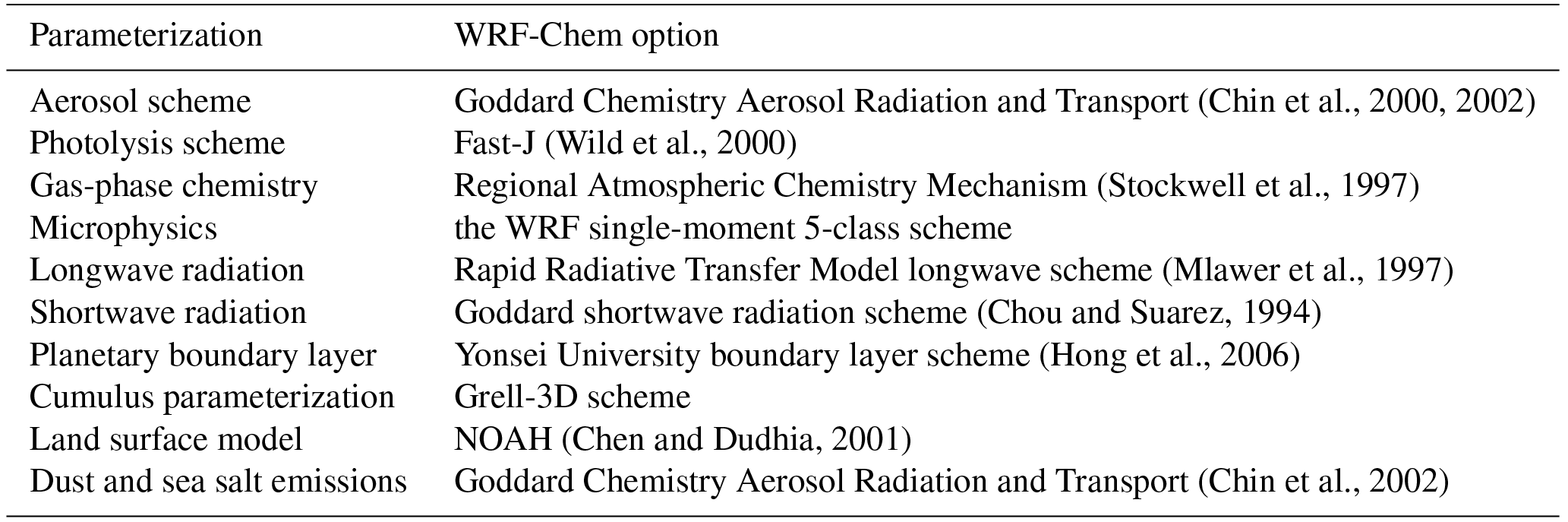
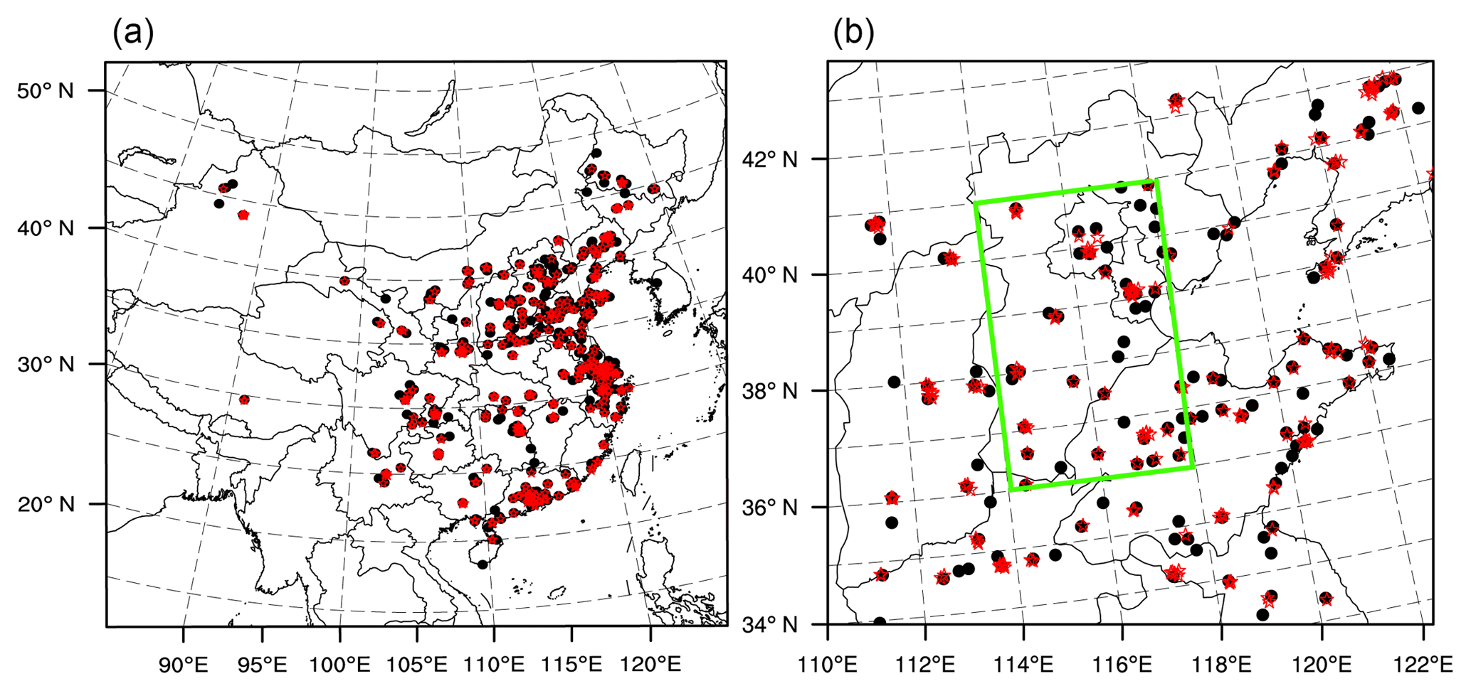
Figure 1 The model domain (a) and the North China Plain (b). Black dots are the observational sites used for assimilation, and red stars are the observational sites used for validation. The green frame marks the Beijing–Tianjin–Hebei region.

2 DA system

The DA system in this study was the same as the one used in Peng et al. (2017). It can simultaneously analyze the chemical ICs and emissions with the assimilation of surface PM_2.5 observations. A brief summary of the DA system is introduced here.

In every DA cycle, the ensemble emission scaling factors λ^f are first calculated by the forecast model of scaling factors M_SF (see details of M_SF in Sect. 2.2). Then, the ensemble forecast emissions E^f are calculated using the following equation:

$$\begin{array}{}\text{(1)}& E_{i,t}={\mathit{\lambda }}_{i,t}{E}_t^{\mathrm{p}},(i=\mathrm{1},\mathrm{\dots },N),\end{array}$$

where $E_t^{\mathrm{p}}$ is the prescribed anthropogenic emission. The ensemble members of chemical fields C^f are forecasted using WRF-Chem, forced by the forecast emissions E^f whose ICs are previously analyzed concentration fields. Now, the background of the joint vector, ${\mathit{x}}^{\mathrm{f}}={\left[C^{\mathrm{f}},{\mathit{\lambda }}^{\mathrm{f}}\right]}^{\mathrm{T}}$, has been produced. Then, the analyzed state vector, ${\mathit{x}}^{\mathrm{a}}={\left[C^{\mathrm{a}},{\mathit{\lambda }}^{\mathrm{a}}\right]}^{\mathrm{T}}$, is optimized using an ensemble square root filter (EnSRF). Finally, the assimilated emissions E^a can be obtained using Eq. (1). It is noted that the optimized emissions are only the results of a mathematical optimum by utilizing observations. If the optimized emissions used in the EnSRF experiment run with pure concentrations as state vectors are identical to the emissions obtained from the joint EnSRF experiment run with concentrations and emission factors (representing emissions) as state vectors, identical results may be obtained.

2.1 WRF-Chem model

The model used to simulate the transport of aerosols and chemical species was the WRF-Chem (Grell et al., 2005). As in Peng et al. (2017), we used version 3.6.1; the physical and chemical parameterization options are listed in Table 1. The model computational domain covered almost the whole of China, and the horizontal resolution was 40.5 km. Figure 1b shows our area of interest, the North China Plain (NCP). The model included 57 vertical levels, and the model top was 10 hPa.

The hourly prior anthropogenic emissions were based on the Multi-resolution Emission Inventory for China (MEIC) (Li et al., 2014) for October 2010, instead of the regional emission inventory in Asia (Zhang et al., 2009) for the year 2006 in Peng et al. (2017). The reason we chose the MEIC-2010 was that the total emissions are reasonable for cities over the NCP (Zheng et al., 2015). The original resolution of the MEIC-2010 is $\mathrm{0.25}{}^{\circ }\times \mathrm{0.25}{}^{\circ }$, but it has been processed to match the model resolution (40.5 km) (Chen et al., 2016). No time variation was added to maintain objectivity in the prior anthropogenic emissions.

2.2 Forecast model of scaling factors

In this work, the primary sources to be optimized were the emissions of PM₁₀, PM_2.5, SO₂, NO, NH₃, and CO. The sources of NH₃ were analyzed because they also impact greatly on the aerosols distribution. Thus, the emission scaling factors ${\mathit{\lambda }}_{i,t}^{\mathrm{f}}=({\mathit{\lambda }}_{{\mathrm{PM}}_{\mathrm{2.5}}}^{\mathrm{f}},{\mathit{\lambda }}_{{\mathrm{PM}}_{\mathrm{10}}}^{\mathrm{f}},{\mathit{\lambda }}_{{\mathrm{SO}}_{\mathrm{2}}}^{\mathrm{f}},{\mathit{\lambda }}_{\mathrm{NO}}^{\mathrm{f}},{\mathit{\lambda }}_{{\mathrm{NH}}_{\mathrm{3}}}^{\mathrm{f}},{\mathit{\lambda }}_{\mathrm{CO}}^{\mathrm{f}})$ were prepared by the forecast model of scaling operator M_SF before WRF-Chem integration.

We used the same persistence forecast operator M_SF to forecast ${\mathit{\lambda }}_{i,t}^{\mathrm{f}}$ as in Peng et al. (2017). The forecast operator was developed by using the ensemble forecast chemical fields. Thus,

$$\begin{array}{}\text{(2)}& {\displaystyle }{\displaystyle }{\mathit{\kappa }}_{i,t}={\displaystyle \frac{C_{i,t}^{\mathrm{f}}}{\stackrel{\mathrm{‾}}{\stackrel{\mathrm{‾}}{C_t^f}}}},(i=\mathrm{1},\mathrm{\dots },N)\end{array}$$

$$\begin{array}{ll}\text{(3)}& {\displaystyle }& {\displaystyle }({\mathit{\kappa }}_{i,t}{)}_{\inf }=\mathit{\beta }\left({\mathit{\kappa }}_{i,t}-\stackrel{\mathrm{‾}}{{\mathit{\kappa }}_t}\right)+\stackrel{\mathrm{‾}}{{\mathit{\kappa }}_t},(i=\mathrm{1},\mathrm{\dots },N)\text{(4)}& {\displaystyle }& {\displaystyle }{\mathit{\lambda }}_{i,t}^{\mathrm{p}}=({\mathit{\kappa }}_{i,t}{)}_{\inf }\text{(5)}& {\displaystyle }& {\displaystyle }{\mathit{\lambda }}_{i,t}^{\mathrm{f}}={\displaystyle \frac{\mathrm{1}}{\mathrm{4}}}\left({\mathit{\lambda }}_{i,t-\mathrm{3}}^{\mathrm{a}}+{\mathit{\lambda }}_{i,t-\mathrm{2}}^{\mathrm{a}}+{\mathit{\lambda }}_{i,t-\mathrm{1}}^{\mathrm{a}}+{\mathit{\lambda }}_{i,t}^{\mathrm{p}}\right),{\displaystyle }& {\displaystyle }(i=\mathrm{1},\mathrm{\dots },N),\end{array}$$

where $C_{i,t}^{\mathrm{f}}$ is the ith ensemble member of the chemical fields at time t, and $\stackrel{\mathrm{‾}}{C_t^{\text{f}}}=\frac{\mathrm{1}}{N}\sum _{i=\mathrm{1}}^N{C}_{i,t}^{\mathrm{f}}$ is the ensemble mean; κ_i,t is the ensemble concentration ratios and $\stackrel{\mathrm{‾}}{{\mathit{\kappa }}_t}$ is the ensemble mean of κ_i,t with values of 1; β is the inflation factor to keep the ensemble spreads of κ_i,t at a certain level; and ${\mathit{\lambda }}_{i,t-\mathrm{1}}^{\mathrm{a}}$, ${\mathit{\lambda }}_{i,t-\mathrm{2}}^{\mathrm{a}}$, and ${\mathit{\lambda }}_{i,t-\mathrm{3}}^{\mathrm{a}}$ are the previous assimilated emission scaling factors. It is noted that ${\mathit{\lambda }}_{i,t}^{\mathrm{f}}$ are spatially varying because they are calculated by using the spatially varying variables, the forecast chemical fields $C_{i,t}^{\mathrm{f}}$. Furthermore, there are very few negative values for (κ_i,t)_inf after inflation. A quality control procedure is performed for (κ_i,t)_inf before further appliance. All these negative data were set as 0 in this work. Then (κ_i,t)_inf were re-centered to ensure the ensemble mean values of (κ_i,t)_inf were all 1. Furthermore, another quality control procedure is performed for ${\mathit{\lambda }}_{i,t}^{\mathrm{a}}$ to keep them positive. Thus, all ${\mathit{\lambda }}_{i,t}^{\mathrm{f}}$ and ${\mathit{\lambda }}_{i,t}^{\mathrm{a}}$ could be positive.

In this study, the ensemble forecast chemical fields of PM₂₅, PM₁₀, SO₂, NO, NH₃, and CO of the previous assimilation cycle are respectively used to calculate the emission scaling factors $({\mathit{\lambda }}_{{\mathrm{PM}}_{\mathrm{2.5}}}^{\mathrm{f}},{\mathit{\lambda }}_{{\mathrm{PM}}_{\mathrm{10}}}^{\mathrm{f}},{\mathit{\lambda }}_{{\mathrm{SO}}_{\mathrm{2}}}^{\mathrm{f}},{\mathit{\lambda }}_{\mathrm{NO}}^{\mathrm{f}},{\mathit{\lambda }}_{{\mathrm{NH}}_{\mathrm{3}}}^{\mathrm{f}},{\mathit{\lambda }}_{\mathrm{CO}}^{\mathrm{f}})$. Previous works (Peng et al., 2015, 2017) showed that reasonable results can be obtained when the ensemble spread of the emission scaling factors range from 0.1 to 1. In order to keep the ensemble spread of the scaling factors at this level in most model area, β is chosen as 1.3, 1.4, 1.3, 1.2, 1.2, and 1.4 for the ensemble concentration ratios of P_2.5, P₁₀, SO₂, NO, NH₃, and CO, respectively, in Eq. (3).

Then, the sources $E_{i,t}^{\mathrm{f}}$ = $(E_{{\text{PM}}_{\mathrm{2.5}}}^{\mathrm{f}}$, $E_{{\text{PM}}_{\mathrm{10}}}^{\mathrm{f}}$, $E_{{\mathrm{SO}}_{\mathrm{2}}}^{\mathrm{f}}$, $E_{\mathrm{NO}}^{\mathrm{f}}$, $E_{{\mathrm{NH}}_{\mathrm{3}}}^{\mathrm{f}}$, $E_{\mathrm{CO}}^{\mathrm{f}})$ are calculated using Eq. (1).

From the perspective of PM_2.5 emissions, these include the unspeciated primary sources of PM_2.5 $E_{{\text{PM}}_{\mathrm{2.5}}}$, sulfate $E_{{\mathrm{SO}}_{\mathrm{4}}}$, and nitrate $E_{{\mathrm{NO}}_{\mathrm{3}}}$. We updated $E_{{\text{PM}}_{\mathrm{2.5}}}$, $E_{{\mathrm{SO}}_{\mathrm{4}}}$, and $E_{{\mathrm{NO}}_{\mathrm{3}}}$ (including the nuclei and accumulation modes) following Peng et al. (2017).

2.3 DA algorithm

The assimilation algorithm employed was the EnSRF proposed by Whitaker and Hamill (2002). The EnKF proposed by Evensen (1994) needs perturbations of observations in practice. Compared to the original EnKF, the EnSRF obviates the need to perturb the observations and avoids additional sampling errors introduced by perturbing observations.

We used the same EnSRF as in Schwartz et al. (2012, 2014). The ensemble member was chosen as 50. The localization radius was chosen as 607.5 km, so EnSRF analysis increments were forced to zero 607.5 km away from an observation (Gaspari and Cohn, 1999). The posterior (after assimilation) multiplicative inflation factor was chosen as 1.2 for all the concentration analysis.

Table 2 State vectors in the data assimilation system.

2.4 State variables

The DA system provides joint analysis of ICs and emissions following Peng et al. (2017). Among them, 16 WRF-Chem/GOCART aerosol variables are included as the state variables. Furthermore, chemical species,such as SO₂, NO₂, and O₃ are also included because they are the most important gas-phase precursors or oxidants of the secondary inorganic aerosols. CO is also assimilated because CO is an important tracer of combustion sources, as well as a precursor of O₃ beyond NO₂ (Parrish et al., 1991). The state variables of the emission scaling factors are $\mathit{\lambda }=({\mathit{\lambda }}_{{\text{PM}}_{\mathrm{2.5}}},{\mathit{\lambda }}_{{\text{PM}}_{\mathrm{10}}},{\mathit{\lambda }}_{{\mathrm{SO}}_{\mathrm{2}}},{\mathit{\lambda }}_{\mathrm{NO}},{\mathit{\lambda }}_{{\mathrm{NH}}_{\mathrm{3}}}{\mathit{\lambda }}_{\mathrm{CO}})$.

Similar to weak-coupling DA, the DA system simultaneously updates both the ICs and the emissions, but with no cross-variable update, in order to avoid the effects of spurious multivariate correlations in the background error covariance that may develop due to the limited ensemble size and errors in both the model and observations (Miyazaki et al., 2012).

For the PM_2.5 observations, the observation operator is expressed as (Schwartz et al., 2012)

$$\begin{array}{ll}\text{(6)}& {\displaystyle }{y}_{{\text{PM}}_{\mathrm{2.5}}}^{\mathrm{f}}=& {\displaystyle }{\mathit{\rho }}_{\mathrm{d}}\left[P_{\mathrm{2.5}}+\mathrm{1.375}S+\mathrm{1.8}\left({\mathrm{OC}}_{\mathrm{1}}+{\mathrm{OC}}_{\mathrm{2}}\right)\right.{\displaystyle }& {\displaystyle }\left.+{\mathrm{BC}}_{\mathrm{1}}+{\mathrm{BC}}_{\mathrm{2}}+D_{\mathrm{1}}+\mathrm{0.286}{D}_{\mathrm{2}}+S_{\mathrm{1}}+\mathrm{0.942}{S}_{\mathrm{2}}\right],\end{array}$$

where ρ_d is the dry-air density; P₂₅ is the fine unspeciated aerosol contributions; S represents sulfate; OC₁ and OC₂ are hydrophobic and hydrophilic organic carbon, respectively; BC₁ and BC₂ are hydrophobic and hydrophilic black carbon, respectively; D₁ and D₂ are dusts with effective radii of 0.5 and 1.4 µm, respectively; and S₁ and S₂ are sea salts with effective radii of 0.3 and 1.0 µm, respectively. In fact, PM_2.5 observations were only used to analyze P_2.5, S, OC₁, OC₂ BC₁, BC₂, D₁, D₂, S₁, S₂, and ${\mathit{\lambda }}_{{\text{PM}}_{\mathrm{2.5}}}$. Since we had no NH₃ observations, PM_2.5 observations were also used to analyze ${\mathit{\lambda }}_{{\mathrm{NH}}_{\mathrm{3}}}$ (see Table 2). For other control variables, PM_2.5 observations were not allowed to alter them.

For the PM₁₀ observations, the PM₁₀ observation operator is expressed as (Jiang et al., 2013)

$$\begin{array}{ll}\text{(7)}& {\displaystyle }{y}_{{\mathrm{PM}}_{\mathrm{10}}}^{\mathrm{f}}=& {\displaystyle }{\mathit{\rho }}_{\mathrm{d}}\left[P_{\mathrm{10}}+P_{\mathrm{2.5}}+\mathrm{1.375}S+\mathrm{1.8}\left({\mathrm{OC}}_{\mathrm{1}}+{\mathrm{OC}}_{\mathrm{2}}\right)\right.{\displaystyle }& {\displaystyle }+{\mathrm{BC}}_{\mathrm{1}}+{\mathrm{BC}}_{\mathrm{2}}+D_{\mathrm{1}}+\mathrm{0.286}{D}_{\mathrm{2}}+D_{\mathrm{3}}+\mathrm{0.87}{D}_{\mathrm{4}}\\ {\displaystyle }& {\displaystyle }\left.+S_{\mathrm{1}}+\mathrm{0.942}{S}_{\mathrm{2}}+S_{\mathrm{3}}\right].\end{array}$$

Thus,

$$\begin{array}{}\text{(8)}& y_{{\text{PM}}_{\mathrm{10}-\mathrm{2.5}}}^{\mathrm{f}}={\mathit{\rho }}_{\mathrm{d}}\left[P_{\mathrm{10}}+D_{\mathrm{3}}+\mathrm{0.87}{D}_{\mathrm{4}}+S_{\mathrm{3}}\right],\end{array}$$

meaning that, in the assimilation experiments, we did not use the PM₁₀ observations directly. In Eqs. (13) and (14), P₁₀ denotes the coarse-mode unspeciated aerosol contributions; D₃ and D₄ are dusts with effective radii of 2.4 and 4.5 µm, respectively; and S₃ is sea salt with an effective radius of 3.25 µm. We used the PM_10−2.5 observations (the differences between the PM₁₀ observations and the PM_2.5 observations, $y_{{\text{PM}}_{\mathrm{10}-\mathrm{2.5}}}^{\mathrm{o}}=y_{{\mathrm{PM}}_{\mathrm{10}}}^{\mathrm{o}}-y_{{\mathrm{PM}}_{\mathrm{10}}}^{\mathrm{o}})$ to analyze P₁₀, D₃, D₄, S₃, and ${\mathit{\lambda }}_{{\text{PM}}_{\mathrm{10}}}$. In addition, PM_10−2.5 observations were used to analyze D₅ and S₄, since they are coarse-mode mineral dust and sea salt aerosols. PM_10−2.5 observations were not allowed to impact other control variables.

Moreover, as shown in Table 2, SO₂ observations were used to analyze the SO₂ concentration and ${\mathit{\lambda }}_{{\mathrm{SO}}_{\mathrm{2}}}$. NO₂ observations were used to estimate the NO, NO₂ concentration and λ_NO. CO observations were used to analyze the CO concentration and λ_CO. And finally, O₃ observations were only used to analyze the O₃ concentration.

3 Observations and errors

The surface chemical observations used in this study were obtained from the Ministry of Ecology and Environment of China. Altogether, there were 876 observational sites over the model domain (Fig. 1). At most sites, one measurement was selected randomly for the assimilation experiment on a $\mathrm{0.1}{}^{\circ }\times \mathrm{0.1}{}^{\circ }$ grid. Altogether, 355 stations were kept for the model domain, where 133 assimilation stations were located on the NCP and 40 stations were located in the Beijing–Tianjin–Hebei (BTH) region. Other stations were used for verification purposes: 167 independent stations were located on the NCP, and 47 in the BTH region.

The observation error covariance matrix R included measurement errors and representation errors. We assumed that R is a diagonal matrix (without observation correlation).

Following Elbern et al. (2007), the measurement error ε₀ is defined as

$$\begin{array}{}\text{(9)}& {\mathit{\epsilon }}_{\mathrm{0}}=a+b\times {\mathrm{\Pi }}_{\mathrm{0}},\end{array}$$

where Π₀ represents the measurements for PM_2.5, PM_10−2.5, SO₂, NO₂, CO, or O₃ (units: µg m⁻³). Values of a=1.5 and b=0.0075 were chosen for PM_2.5, PM_10−2.5, SO₂, and NO₂. For CO, a=10 and b=0.0075.

The representativeness error is defined as

$$\begin{array}{}\text{(10)}& {\mathit{\epsilon }}_{\text{r}}=r{\mathit{\epsilon }}_{\mathrm{0}}\sqrt{\mathrm{\Delta }x}/\mathrm{L},\end{array}$$

where r=0.5, Δx=40.5 km (the model resolution), and L=3 km due to the lack of the information of the station type (Elbern et al., 2007).

Finally, the total error (ε_t) is defined as

$$\begin{array}{}\text{(11)}& {\mathit{\epsilon }}_{\mathrm{t}}=\sqrt{{\mathit{\epsilon }}_{\mathrm{0}}^{\mathrm{2}}+{\mathit{\epsilon }}_{\text{r}}^{\mathrm{2}}}.\end{array}$$

In order to ensure data reliability, the observations were subjected to quality control before DA. Data values larger than a certain threshold were classified as unrealistic and were not assimilated. The threshold values were chosen as 700, 800, 300, 300, 400, and 4000 µg m⁻³ for PM_2.5, PM_10−2.5, SO₂, NO₂, O₃, and CO, respectively. In addition, observations leading to innovations exceeding a certain value were also omitted. These threshold values were chosen as 70 µg m⁻³ for PM_2.5, PM_10−2.5, SO₂, NO₂, and O₃. Also, 1500 µg m⁻³ was chosen for CO.

Figure 2 Time series of prior ensemble mean RMSE (blue line) and total spread (black line) for PM_2.5, PM₁₀, SO₂, NO₂, CO, and O₃ concentrations aggregated over all observations over the Beijing–Tianjin–Hebei region. Units for all these variables: µg m⁻³.

4 Experimental design

The DA experiment followed that of Peng et al. (2017), in which the assimilation of pure surface PM_2.5 measurements with the EnKF was performed to correct finer aerosol variables and associated emissions. The experiment focused on an extreme haze event that occurred in October 2014 over northern China.

The 50-member ensemble spin-up forecasts were first performed from 1 to 4 October 2014 using the perturbed meteorological ICs, lateral boundary conditions (LBCs), and emissions. The perturbed meteorological ICs and LBCs are created by adding Gaussian random noise (Torn et al., 2006) to the temperature, water vapor, velocity, geopotential height, and dry surface pressure fields of the products of the National Centers for Environmental Prediction Global Forecast System (GFS) by WRFDA. The perturbed emissions were generated also by adding Gaussian random noise with a standard deviation of 10 % of the corresponding anthropogenic emissions. The aerosol ICs were zero, and the aerosol LBCs were idealized profiles embedded within the WRF-Chem model; neither of them was perturbed (Peng et al., 2017).

Then, the observed PM₁₀, PM_2.5, SO₂, NO₂, O₃, and CO data starting from 5 to 16 October were assimilated hourly to adjust the ICs and the corresponding emissions. The ICs were the subject of analysis of the previous DA cycle. The meteorological LBCs were perturbed. The anthropogenic emissions – $E_{{\text{PM}}_{\mathrm{2.5}}}$, $E_{{\text{PM}}_{\mathrm{10}}}$, $E_{{\mathrm{SO}}_{\mathrm{2}}}$, E_NO, $E_{{\mathrm{NH}}_{\mathrm{3}}}$, E_CO, $E_{{\mathrm{SO}}_{\mathrm{4}}}$, and $E_{{\mathrm{NO}}_{\mathrm{3}}}$ – are calculated by using the forecast emission scaling factors. Other species, such as the organic compounds E_org and elemental compounds E_BC, are perturbed by adding Gaussian random noise. Since the emissions are calculated by Eq. (1), their background uncertainties and the spatial correlations are completely dependent on those of the corresponding emission factors. The forecast scaling factors are calculated by Eqs. (2)–(5). And no other perturbations are added to the scaling factors; no other correlations are assumed for the scaling factors.

After that, two sets of 72 h forecasts were performed, each at 00:00 UTC from 6 to 15 October 2014, with hourly forecasting outputs for the assimilation experiment. These two sets of forecasting experiments were conducted using the ensemble mean of the concentration analysis as the ICs. One set of the experiments was forced by the optimized emissions (denoted as fcICsEs), and the other was forced by the prescribed anthropogenic emissions (denoted as fcICs). The aim was to use the difference between the fcICsEs and fcICs to indicate the impact of the optimized emissions.

Moreover, we also ran a control experiment. The ICs were based on the ensemble mean of the spin-up forecasts at 00:00 UTC on 5 October 2014. The emissions were the prescribed emissions.

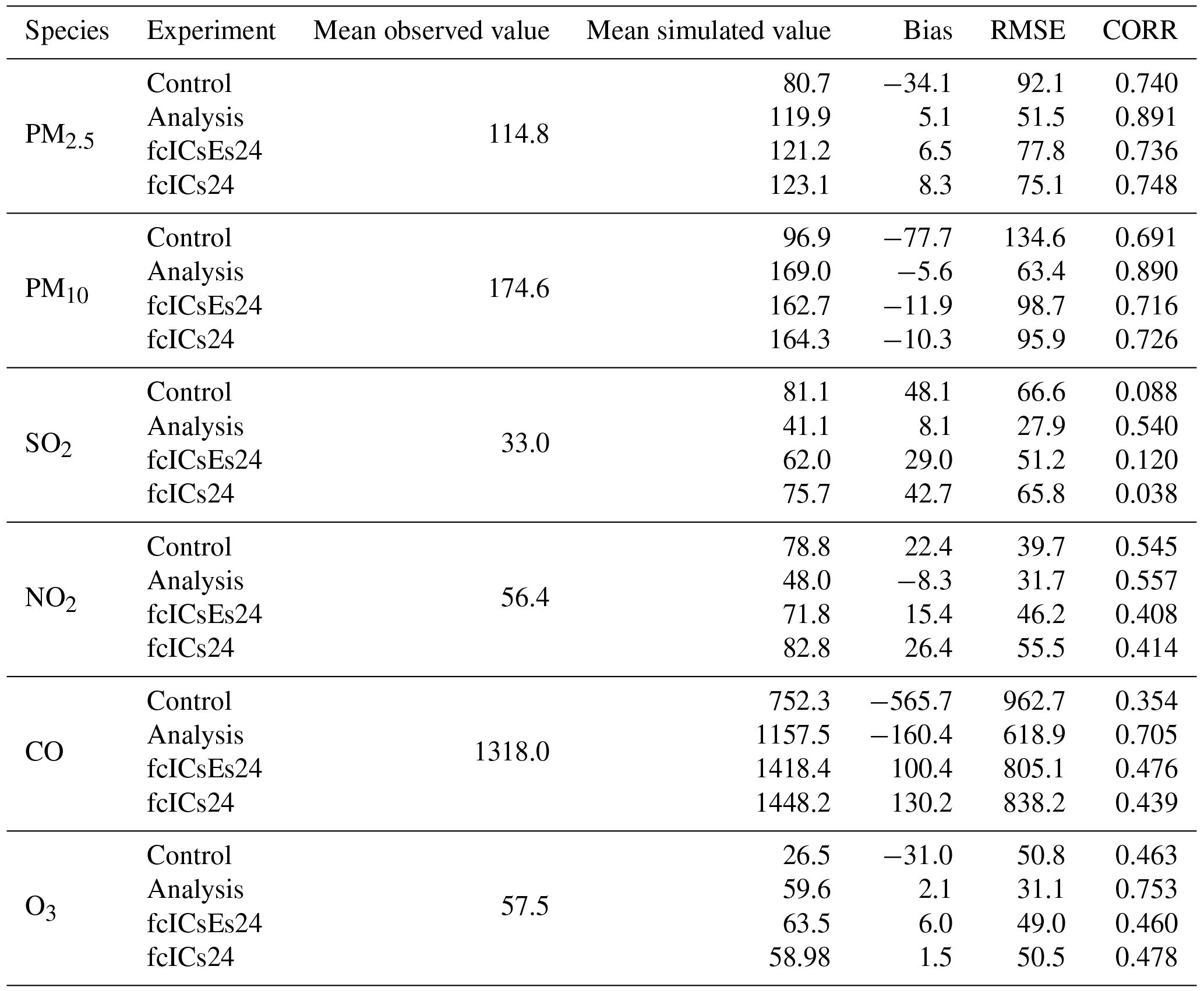
Table 3 Comparison with observations of the surface PM_2.5 mass concentrations in the Beijing–Tianjin–Hebei region from the control experiment, the assimilation experiment, and the first-day forecast, over all analysis times from 6 to 16 October 2014. Units: µg m⁻³.

5 Results

5.1 Ensemble performance

We begin by assessing the ensemble performance for the DA system. Figure 2 shows the time series of the prior total spreads and the prior root-mean-square errors (RMSEs) for PM_2.5, PM₁₀, and the four trace gases calculated against all observations in the BTH region. It shows that the magnitudes of the total spreads were close to the RMSEs, indicating that the DA system was well calibrated (Houtekamer et al., 2005).

Figure 3 shows the area-averaged time series extracted from the ensemble spread of the six emission scaling factors (${\mathit{\lambda }}_{{\text{PM}}_{\mathrm{2.5}}}^{\mathrm{f}}$, ${\mathit{\lambda }}_{{\text{PM}}_{\mathrm{10}}}^{\mathrm{f}}$, ${\mathit{\lambda }}_{{\mathrm{SO}}_{\mathrm{2}}}^{\mathrm{f}}$, ${\mathit{\lambda }}_{\mathrm{NO}}^{\mathrm{f}}$, ${\mathit{\lambda }}_{{\mathrm{NH}}_{\mathrm{3}}}^{\mathrm{f}}$, and ${\mathit{\lambda }}_{\mathrm{CO}}^{\mathrm{f}})$ in the BTH region. It shows that the ensemble spread of all the scaling factors were very stable throughout the ∼10-day experiment period, which indicates that M_SF can generate stable artificial data to generate the ensemble emissions. The value of the emission scaling factors ranged from 0.2 to 0.6, indicating that the uncertainty of the assimilated emissions was about 20 %–60 %.

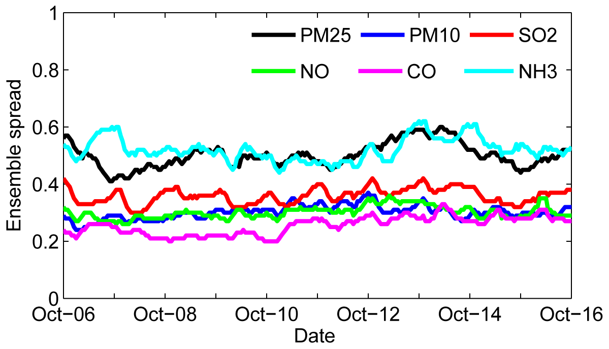
Figure 3 Time series of the area-averaged ensemble spread for the emission scaling factors over the Beijing–Tianjin–Hebei region.

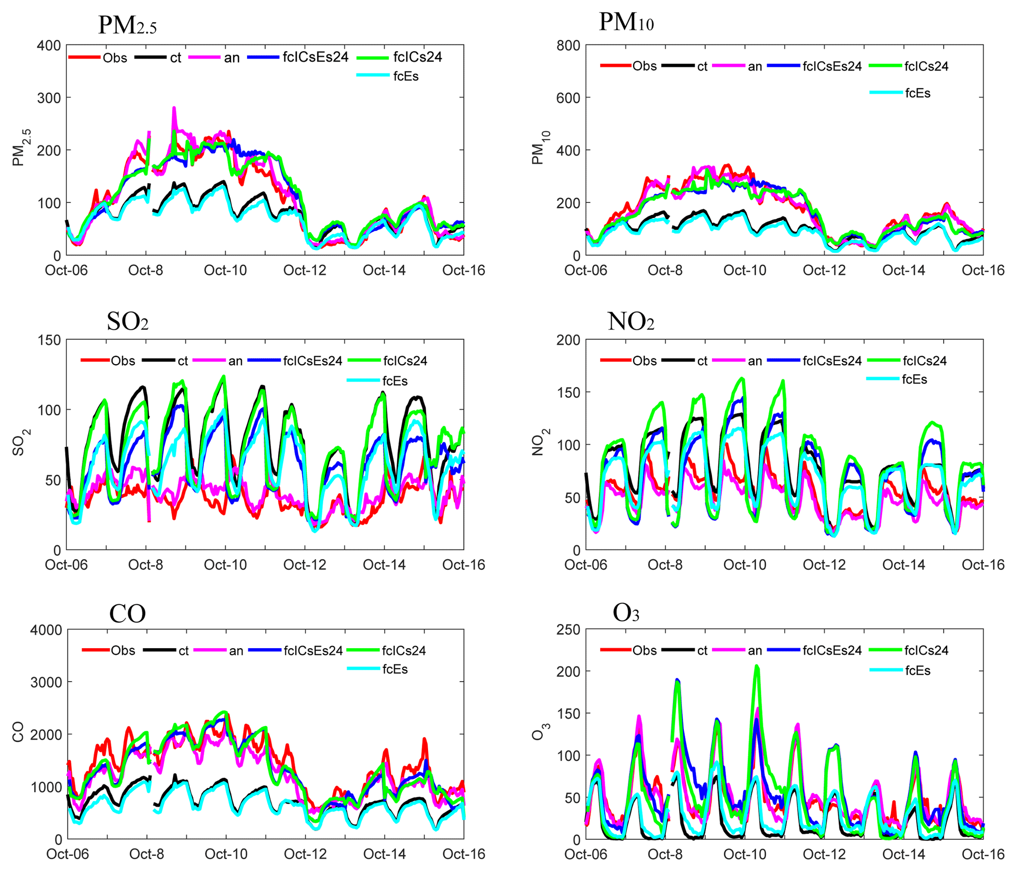
Figure 4 Time series of the hourly pollutant concentrations in the Beijing–Tianjin–Hebei (BTH) region obtained from observations (red line), the control run (black line), the analysis (pink line), the first-day forecast from fcICsEs (fcICsEs24, blue line), and the first-day forecast from fcICs (fcICs24, blue line). The observations were obtained from the 47 independent sites in the BTH region. The modeled time series were interpolated to the 47 independent sites using the spatial bilinear interpolator method. The shaded backgrounds indicate the distribution of the observations, where the top edge represented the 90th percentile and the bottom edge the 10th percentile. Units: µg m⁻³.

5.2 Forecast improvements

In order to evaluate the overall performance of the DA system, time series of the hourly pollutant concentrations from the control run, the analysis, and the first-day forecast of the two forecasting experiments were compared with the independent observations in the BTH region (Fig. 4). Furthermore, model evaluation statistics (Table 3) were calculated against independent observations from 6 to 16 October 2014. In addition, biases and RMSEs were presented as a function of forecast range for the control, analysis, and forecast experiments (Figs. 5–7).

The control run did not perform very well, although it was able to capture the synoptic variability and reproduce the overall pollutant levels when there was a severe haze event. The statistics show that there were larger systematic biases and RMSEs and a smaller correlation coefficient (CORR) for the control (see Table 3). The biases were −34.1, −77.7, −565.7, and −31 µg m⁻³ for PM_2.5, PM₁₀, CO, and O₃, respectively, from 6 to 16 October – about 29.7 %, 44.5 %, 42.9 %, and 53.9 % lower than the corresponding observed concentrations. During the severe haze episode from 8 to 10 October in particular, when observed PM_2.5 were larger than 200 µg m⁻³, the biases reached −90.5, −143.1, −911.8, and −39.1µg m⁻³, respectively – about 44.4 %, 51.9 %, 49.2 % and 55.7 % lower than the corresponding observed concentrations, suggesting a significant systematic underestimation of the WRF-Chem simulation. Additionally, a significant overestimation of 48.1 µg m⁻³ was obtained for SO₂ – about 145.8 % higher than the observed concentrations. As for the NO₂ simulation, WRF-Chem was able to realistically describe the diurnal and synoptic evolution of NO₂ concentrations. The model bias was 22.4 µg m⁻³, which was about 39.7 % higher than the observed NO₂. These results were similar to the simulations of Chen et al. (2016). Most of the WRF-Chem settings used here were the same as those used in Chen et al. (2016), except that they used CBMZ (Carbon Bond Mechanism, version Z) and MOSAIC (Model for Simulating Aerosol Interactions and Chemistry) as the gas-phase and aerosol chemical mechanisms.

Figure 5 Bias of surface PM_2.5, PM₁₀, SO₂, NO₂, CO, and O₃ as a function of forecast range calculated against all the independent observations over the Beijing–Tianjin–Hebei region shown in Fig. 1. The 72 h forecasts were performed at each 00:00 UTC from 6 to 14 October 2014, and the statistics were computed from 6 to 14 October. Units: µg m⁻³.

After the assimilation of surface observations, the time series of the hourly pollutant concentrations from the analysis showed much better agreement with observations than those from the control. The magnitudes of the bias and the RMSEs decreased, and the CORRs increased for all six species. The biases were 5.1, −5.6, 8.1, −8.3, −160.4, and 2.1 µg m⁻³ for PM_2.5, PM₁₀, SO₂, NO₂, CO, and O₃, respectively – about 4.4 %, −3.2 %, 24.5 %, −14.7 %, −12.17 %, and 3.7 % of the corresponding observed concentrations, indicating that the analysis fields were very close to the observations. The RMSEs were 51.5, 63.4, 27.9, 31.7, 618.9, and 31.1 µg m⁻³, respectively – about 44.1 %, 52.9 %, 58.1 %, 20.2 %, 35.7 %, and 38.78 % lower than the RMSEs of the control run. The CORRs reached 0.891, 0.890, 0.540, 0.557, 0.705, and 0.753, respectively. These statistics indicate that the DA system was able to adjust the chemical ICs efficiently.

The PM_2.5, PM₁₀, and CO concentrations from both sets of forecasting experiments benefitted substantially from the DA procedure, as expected. Smaller biases and RMSEs were obtained for almost the entire 72 h forecast range (see Figs. 5–7), as compared with the control run. For the first-day forecast in particular, the model performed almost perfectly. It faultlessly captured the diurnal and synoptic variability of the pollutant (see Fig. 4), in a manner that was very close to that of the analysis. The overall biases were 6.5, −11.9, and 100.4 µg m⁻³ for PM_2.5, PM₁₀, and CO, respectively, and the RMSEs were 77.8, 98.7, and 805.1 µg m⁻³, respectively, in fcICsEs24 (see Table 3). In fcICs24, the biases were 8.3, −10.3, and 130.2 µg m⁻³, respectively, and the RMSEs were 75.1, 95.9, and 838.2 µg m⁻³, respectively (see Table 3). However, with longer-range forecasts, the impact of DA quickly decayed. The relative reductions in RMSE mostly ranged from 30 % to 5 % for the second- and third-day forecast. From the perspective of the impact of the assimilated emissions, fcICs performed similarly to fcICsEs for PM_2.5, PM₁₀, and CO, indicating that ICs play key roles in aerosol and CO forecasts during severe haze episodes, while the impact of assimilated emissions seems negligible.

Figure 6 As in Fig. 5 but for RMSE. Units: µg m⁻³.

For the SO₂ verification forecast, however, fcICsEs performed much better than both fcICs and the control run. Smaller biases and RMSEs were obtained for almost the entire 72 h forecast range. At nighttime in particular (from 18 to 23 h, 42 to 47 h, and 66 to 73 h), when there was significant systematic overestimation in the control run, both the biases and the RMSEs in fcICsEs were about 30 % lower than those of the control run. During the daytime (from 0 to 9 h, 24 to 33 h, and 48 to 57 h), fcICsEs still performed slightly better, although the control run did a near-perfect job. As for fcICs, smaller biases and RMSEs were obtained for only the first 3 h. Then, the performance was the same as the control run, indicating that the impact of the ICs had disappeared. These results demonstrate the superiority of the assimilated emissions, and that the joint adjustment of SO₂ ICs and emissions is an efficient way to improve the SO₂ forecast.

The NO₂ DA results for the independent sites showed really poor performance (see Figs. 5–7). Smaller biases were gained in the daytime of the experiment trials. At nighttime, however, when the simulated NO₂ deviated considerably from the observations in the control run, the biases of both sets of the validation forecasts became even larger. Furthermore, almost all the RMSEs of both sets of the validation forecasts were always larger than those of the control run.

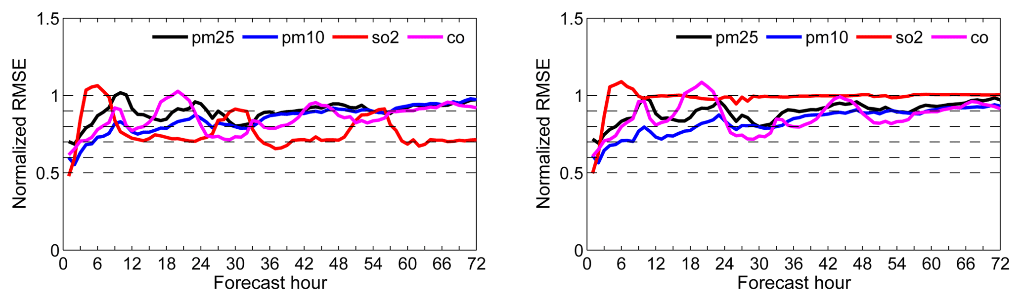
Figure 7 Normalized RMSE (assimilation divided by control) for fcICsEs and fcICs for PM_2.5, PM₁₀, SO₂, and CO.

The O₃ DA results were dependent on the NO₂ DA results in the daytime, due to chemical transformation. Both the biases and the RMSEs were larger, as compared with those of the control run (see Figs. 5–7). However, at nighttime, when there was significant systematic underestimation in the control run, the biases in fcICsEs had very similar values to those of the analysis. Also, the biases in fcICs ranged between the analysis and the control run, and the RMSEs of both sets of forecasting experiments were about 10 % smaller than those of the control run. All these results indicate that the DA system performed well at night.

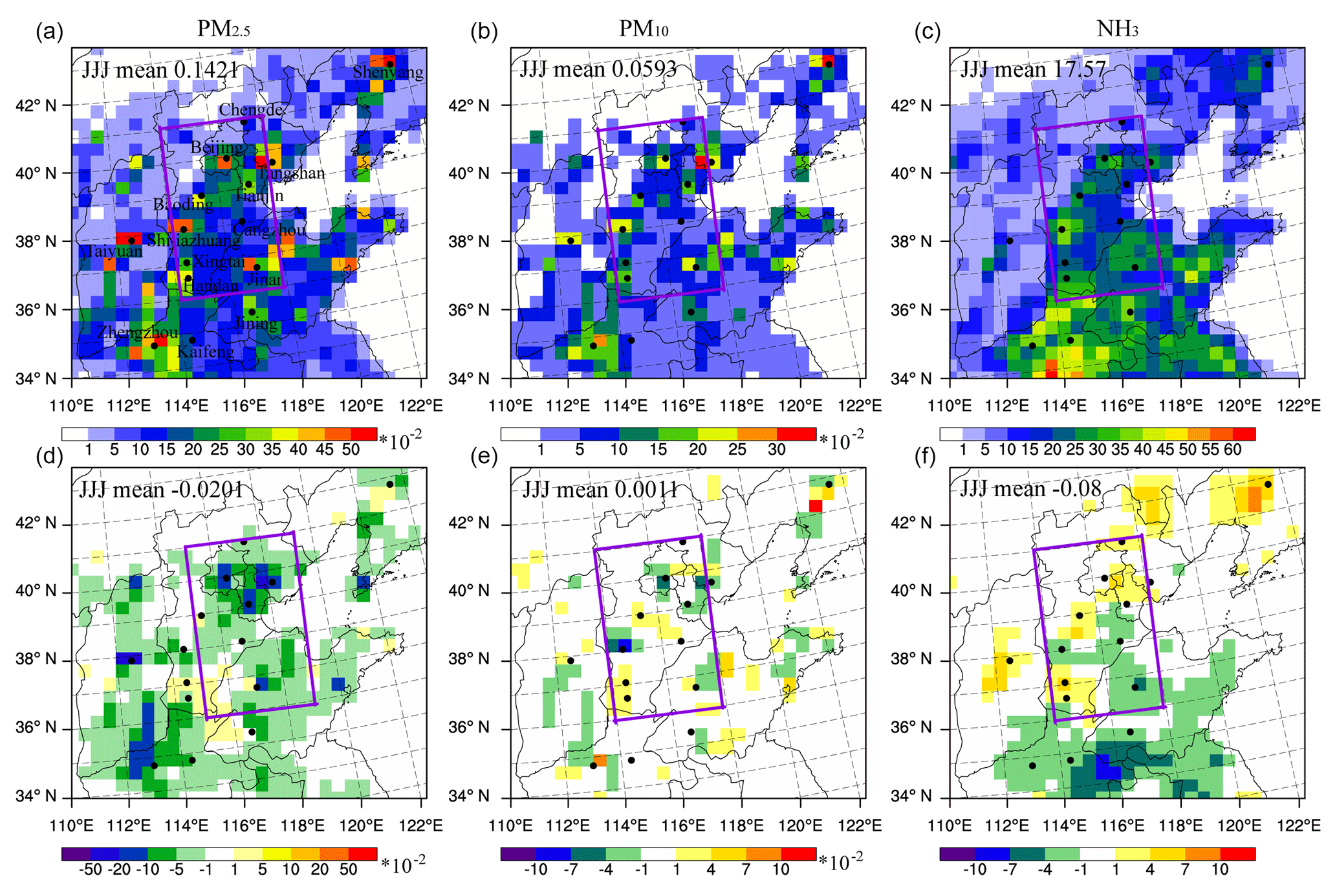
Figure 8 Spatial distribution of the prescribed emissions (top panels) of PM_2.5 (a, d), PM₁₀ (b, e), and NH₃ (c, f) and the corresponding time-averaged differences between the ensemble mean analysis and the prescribed values at the lowest model level averaged over all hours from 6 to 16 October 2014 in the NCP region. Units for PM_2.5 and PM₁₀ emissions: µg m⁻² s⁻¹; units for NH₃ emissions: mol km⁻² h⁻¹.

5.3 Emission optimization results

Besides improved pollutant forecasts, improved estimates of emissions were expected from the joint DA procedure. The MEIC-2010 was constructed on the basis of annual statistical books in which the data were often 2–3 years older than the actual year (Chen et al., 2016). However, consistent efforts aimed at reducing and managing anthropogenic emissions have been made over the past decade to mitigate air pollution. Thus, there was a large difference between the emission year and our simulation year. Furthermore, the spatial allocations of these emissions over small spatial scales, and the monthly allocations, will also lead to some uncertainties. Lastly, the emissions inventory cannot fully capture the day-to-day variability or the actual daily variations, though its differentiation in terms of working days and weekend days, plus the daily variations, can be taken into account in practical applications. However, in this assimilation procedure, the differentiation in terms of working days and weekend days, plus the daily variations, was ignored. Therefore, the prescribed anthropogenic emissions were subject to large uncertainties.

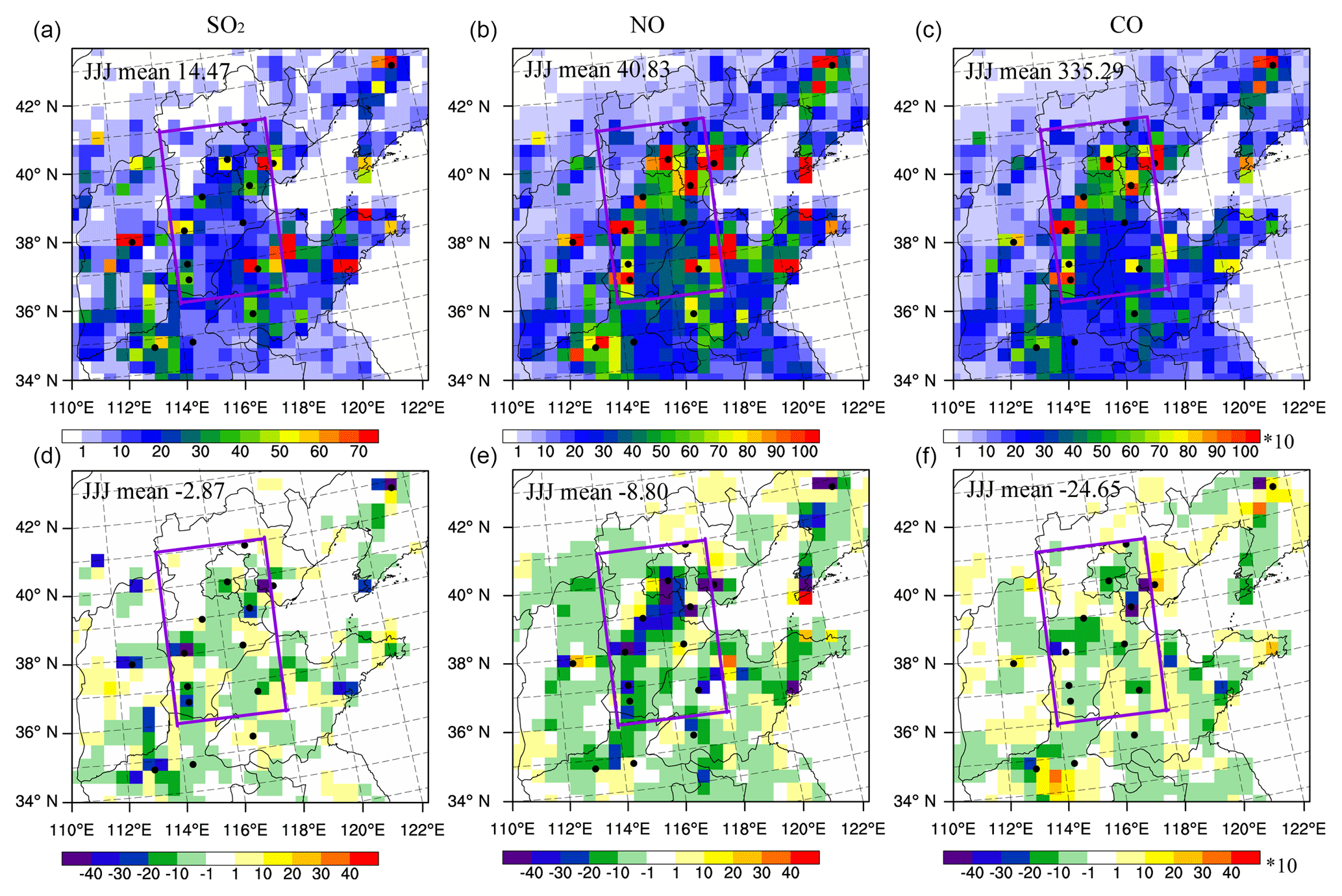
Figure 9 As in Fig. 8 but for SO₂ (a, d), NO (b, e), and CO (c, f). Units for SO₂, NO, and CO emissions: mol km⁻² h⁻¹.

Figures 8 and 9 display the spatial distribution of the prescribed emission rates and the differences between the analysis and the prescribed emission rates of PM_2.5, PM₁₀, NH₃, SO₂, NO, and CO averaged over all hours from 6 to 16 October 2014 in the NCP region. The assimilated emission rates of PM_2.5, SO₂, NO, and CO were lower than the prescribed emissions on the whole. In the BTH region especially, the differences reached −0.02 µg m⁻² s⁻¹, −2.9, −8.8, and −24.65 mol km⁻² h⁻¹, which was a reduction of about 10 %–20 % of the prescribed emissions. For PM₁₀ emissions, the assimilated values were very close to the prescribed ones, indicating that the prescribed PM₁₀ emissions had small uncertainties for the NCP region. For NH₃ emissions, the assimilated values were a little larger than the prescribed emissions in large industrial cities like Beijing, Tianjin, Baoding, Xingtai, Handan, and Taiyuan. However, they were smaller than the prescribed emissions in agricultural regions, especially in Shandong and Henan provinces. However, in the BTH region, the assimilated NH₃ emissions were very close to the prescribed emissions on the whole.

Figure 10 shows the time series of the emission scaling factors and the emissions. As concluded in Peng et al. (2017), the forecast emission scaling factors changed with the analyzed emission scaling factors due to the use of the time-smoothing operator. Furthermore, although the prescribed emissions were constant when designing the assimilation experiment, the analyzed emission scaling factors showed obvious variation with time, as did the analyzed emissions. For the assimilated SO₂ and NO emissions in particular, the diurnal variations were perfect. In addition, the difference between the assimilated emissions and the prescribed emissions were consistent with those in Figs. 8 and 9. The assimilated emissions of PM_2.5, SO₂, NO, and CO were apparently lower than the corresponding prescribed emissions, whereas the values of the assimilated emissions of PM₁₀ and NH₃ were very close to their corresponding prescribed emissions.

In order to investigate the impact of optimized emissions on chemical simulations, a simulation (fcEs) using the optimized emissions was performed from 5 to 16 October 2014. Just as in the control run, the ICs were the ensemble mean of the spin-up forecasts at 00:00 UTC on 5 October 2014. Thus the difference between the fcEs and the control run is the anthropogenic emissions. The results showed that the fcEs performed very similarly to the control run on the whole in the BTH region. For PM_2.5, PM₁₀, and CO, the values of the fcEs were a little smaller than those of the control run, which were consistent with the difference of the anthropogenic emissions. For SO₂ and NO₂, fcEs performed much better than the control run most of the time, though significant systematic overestimation still existed during the nighttime. For O₃, minor improvements were also gained due to the better simulation in fcEs for NO₂.

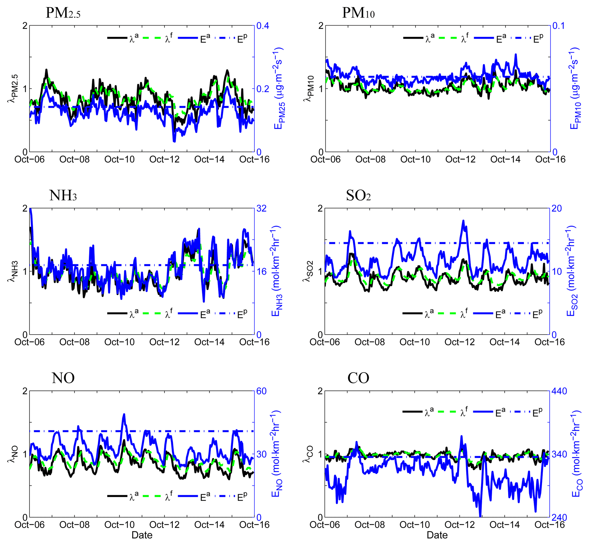
Figure 10 Hourly area-averaged time series extracted from the analyzed emission scaling factors (black line), the forecast emission scaling factors (green dashed line), the analyzed emissions (blue line), and the prescribed emissions (blue dashed line) in the Beijing–Tianjin–Hebei region. Units for PM_2.5 and PM₁₀ emissions: µg m⁻² s⁻¹; units for NH₃, SO₂, NO, and CO emissions: mol km⁻² h⁻¹.

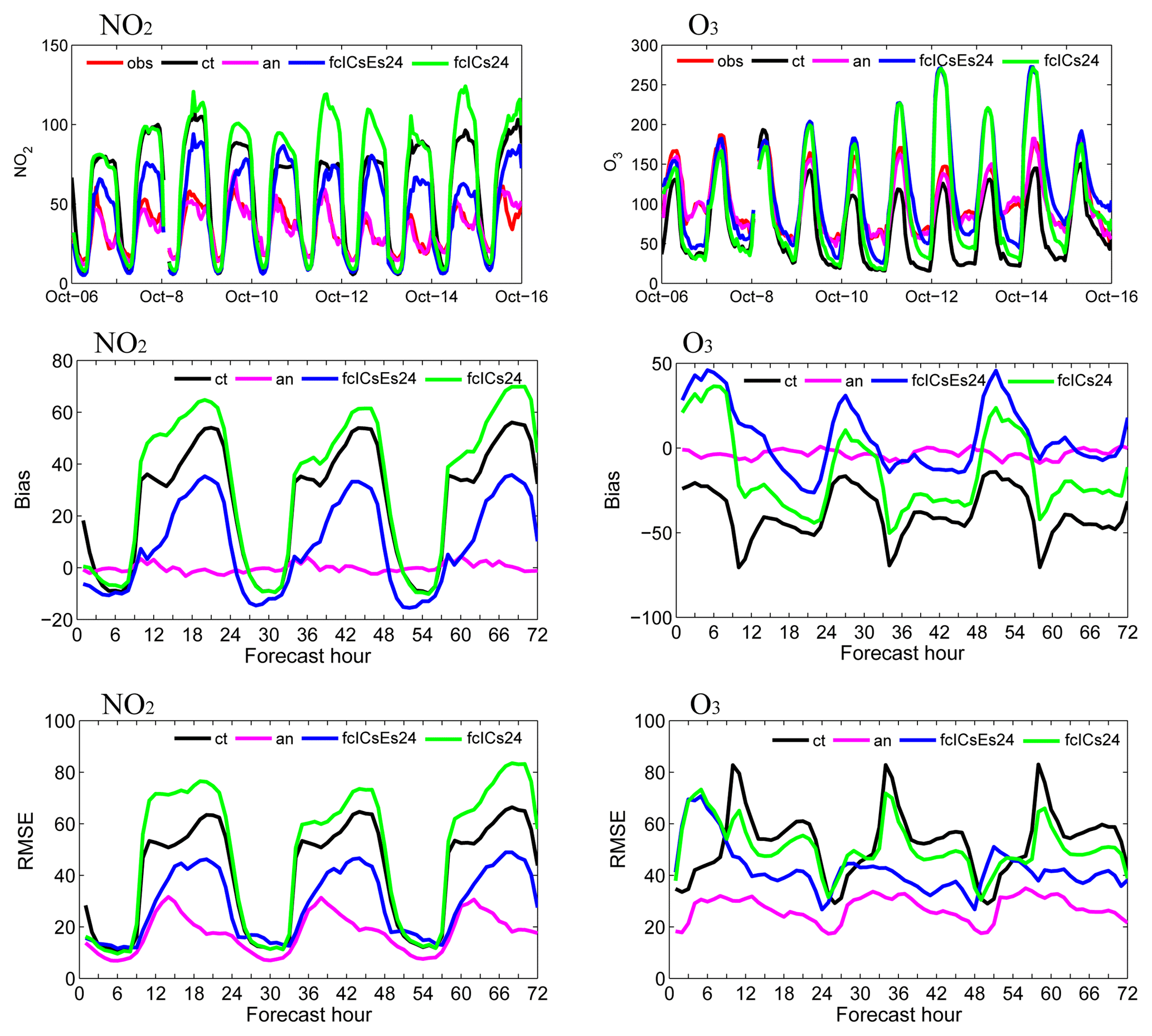
Figure 11 NO₂ and O₃ time series of the hourly pollutant concentrations in the Pearl River delta region (PRD; 21–24^∘ N, 112.5–115^∘ E) obtained from observations (referred to as “obs”, red line), the control run (referred to as “ct”, black line), the analysis (referred to as “an”, pink line), the first-day forecast from fcICsEs (referred to as “fcICs24”, blue line), and the first-day forecast from fcICs (referred to as “fcICs24”, blue line). The bias and RMSEs of surface NO₂ and O₃ as a function of forecast range calculated against all the independent observations (34 sites) over the PRD region. Units: µg m⁻³.

5.4 Discussion

From the results presented above, it is clear that improvements were achieved for almost all the 72 h verification forecasts using the optimized ICs and emissions for PM_2.5, PM₁₀, SO₂, and CO concentrations in the BTH region. However, the 72 h NO₂ verification forecasts performed much worse than the control run, due to the assimilation. Plus, the 72 h O₃ verification forecasts performed worse than the control run during the daytime, due to the worse performance of the NO₂ forecasts, although they did perform better at night. However, relatively favorable NO₂ and O₃ forecast results were gained for the Yangtze River delta and Pearl River delta (PRD) regions (see Fig. 11). In the PRD region, during the daytime, the three NO₂ forecasts (i.e., the control run, the fcICsEs, and the fcICs) performed similarly and had relatively small biases and RMSEs. At nighttime, when there was significant systematic overestimation in the control run, the biases and the RMSEs in fcICsEs were much smaller than those in the control run. For the O₃ 72 h verification forecasts, fcICsEs performed much better than the control run, except for the first 8 h. Also, fcICs improved the O₃ forecasts to some extent in the 9–72 h forecast range. These results indicate that DA is still an effective way to improve NO₂ and O₃ forecasts.

Regarding the failure to improve the NO₂ and O₃ forecasts in the BTH region, there are three likely factors. Certainly, NO₂ and O₃ forecasts in other areas are also facing similar challenges.

Firstly, there are still some limitations for the EnKF method. EnKF assimilation is influenced greatly by model errors and observation errors. There are many sources of uncertainties in air quality forecasts that were not directly considered in this study (such as chemical schemes and parameterizations, meteorology, and emissions). And it is very difficult to accurately evaluate the uncertainties of models, though the covariance inflation technique was simply applied for all state variables to roughly compensate for model errors. Therefore, we can only obtain suboptimal results through EnKF assimilation. Furthermore, short-lived chemical reactive species, such as NO₂ and O₃, undergo highly complex nonlinear photochemical reactions, even on timescales of hours, such that the forecast accuracy is largely dependent on the chemical process as well as the physical transportation process, the ICs, and the emissions. However, those complex photochemical reaction processes are not precisely described in current chemical mechanisms, e.g., heterogeneous reactions (Yang et al., 2015), the photolysis of nitrous acid and ClNO₂ during daytime (Zhang et al., 2017), and so on. Therefore, on the one hand, there are still large uncertainties for NO₂ and O₃ forecasts, while, on the other hand, it is very difficult for NO₂ and O₃ DA to accurately estimate the model errors with a limited ensemble size. Thus, NO₂ and O₃ assimilations do not perform well (Elbern et al., 2007; Tang et al., 2016). However, for SO₂ and CO, which are representative of long-lived chemical reactive species, the chemical reaction process does not work on timescales of hours, meaning that to some extent hourly chemical DA has the potential to improve their forecasts. For CO in particular, due to its inertness, we might be able to obtain high-quality ICs and emissions through DA. The primary sources of aerosol are the dominant part of the atmospheric aerosol concentration. So, 72 h aerosol forecasts may perform similarly to CO, although there are large uncertainties in the chemical model.

Secondly, as stated in the above paragraph, the analysis ICs and emissions are only a mathematical optimum under the existing conditions. In addition, only part of the chemical ICs and emissions are involved in the DA experiment; VOC ICs and emissions, which may greatly influence the NO₂ and O₃ forecasts, were not included here because of the absence of VOC measurements. Although we carried out two DA sensitivity experiments to adjust the VOC ICs and emissions through the use of NO₂ or O₃ measurements, we were still unable to gain improved NO₂ and O₃ forecasts in the BTH region in both DA experiments. VOC measurements are needed to reduce uncertainties of VOC ICs and emissions. In addition, almost all available data were observed in cities, and no observation stations were located in rural areas. Thus, the atmospheric environmental monitoring system was still spatially heterogeneous.

Another important point is that there are still limitations to the current chemical mechanisms used in our model, such as the treatment of model error. NO is the primary species of NO_x emissions in city areas and reacts directly with O₃ to form NO₂ ($\mathrm{NO}+{\mathrm{O}}_{\mathrm{3}}\to {\mathrm{NO}}_{\mathrm{2}}+{\mathrm{O}}_{\mathrm{2}}$). Thus, O₃ concentrations may inversely correlate with NO₂ concentrations at night. Consequently, air quality models may systematically underestimate O₃ concentrations. Currently, DA can only revise the ICs and the emissions in this work. It cannot change the model performance, especially when there are certain uncertainties for the meteorological simulation.

6 Summary

In this study, we developed an EnKF system to simultaneously assimilate surface measurements of PM₁₀, PM_2.5, SO₂, NO₂, O₃, and CO via the joint adjustment of ICs and source emissions. This system was applied to assimilate hourly pollution data while modeling an extreme haze event that occurred in early October 2014 over northern China. In order to evaluate the impact of DA, two sets of 72 h verification forecasts were performed. One was conducted with the optimized ICs and emissions, and the other with only optimized ICs and the prescribed emissions. A control experiment without DA was also performed for comparison.

The results showed that both verification forecasts performed much better than the control simulations for PM_2.5, PM₁₀, and CO. Obvious improvements were achieved for almost the entire 72 h forecast range. For the first-day forecast especially, near-perfect forecasts results were achieved. However, with longer-range forecasts, the impact of DA quickly decayed. In addition, the forecasts with only optimized ICs and the prescribed emissions performed similarly to those with the optimized ICs and emissions, indicating that ICs play key roles in PM_2.5, PM₁₀, and CO forecasts during severe haze episodes.

Also, large improvements were achieved for SO₂ forecasts with both the optimized ICs and emissions for the whole 72 h forecast range. However, similar improvements were achieved for SO₂ forecasts with the optimized ICs only for the first 3 h, and then the impact of the ICs decayed quickly to zero. This demonstrates that the joint adjustment of SO₂ ICs and emissions is an efficient way to improve SO₂ forecasts.

Even though we failed to improve the NO₂ and O₃ forecasts in the BTH region, relatively favorable NO₂ and O₃ forecast results were gained in other areas. Also, the forecasts with both the optimized ICs and emissions performed much better than the forecasts with only optimized ICs and the prescribed emissions. These results indicate that there is still potential to improve NO₂ and O₃ forecasts via the joint adjustment of SO₂ ICs and emissions.

However, only one case was investigated in this work. Thus it is uncertain if the conclusions about different performance of forecasts for various species would hold in a general. Therefore, more case studies are needed to obtain general conclusions in future works.