the Creative Commons Attribution 4.0 License.
the Creative Commons Attribution 4.0 License.
 | 17 Oct 2018
Seasonal evaluation of tropospheric CO2 over the Asia-Pacific region observed by the CONTRAIL commercial airliner measurements
Hidekazu Matsueda
Yousuke Sawa
Yosuke Niwa
Toshinobu Machida
Lingxi Zhou
Measurement of atmospheric carbon dioxide (CO2) is indispensable for top-down estimation of surface CO2 sources/sinks by an atmospheric transport model. Despite the growing importance of Asia in the global carbon budget, the region has only been sparsely monitored for atmospheric CO2 and our understanding of atmospheric CO2 variations in the region (and thereby that of the regional carbon budget) is still limited. In this study, we present climatological CO2 distributions over the Asia-Pacific region obtained from the CONTRAIL (Comprehensive Observation Network for TRace gases by AIrLiner) measurements. The high-frequency in-flight CO2 measurements over 10 years reveal a clear seasonal variation in CO2 in the upper troposphere (UT), with a maximum occurring in April–May and a minimum in August–September. The CO2 mole fraction in the UT north of 40∘ N is low and highly variable in June–August due to the arrival of air parcels with seasonally low CO2 caused by the summertime biospheric uptake in boreal Eurasia. For August–September in particular, the UT CO2 is noticeably low within the Asian summer monsoon anticyclone associated with the convective transport of strong biospheric CO2 uptake signal over South Asia. During September as the anticyclone decays, a spreading of this low-CO2 area in the UT is observed in the vertical profiles of CO2 over the Pacific Rim of continental East Asia. Simulation results identify the influence of anthropogenic and biospheric CO2 fluxes in the seasonal evolution of the spatial CO2 distribution over the Asia-Pacific region. It is inferred that a substantial contribution to the UT CO2 over the northwestern Pacific comes from continental East Asian emissions in spring; but in the summer monsoon season, the prominent air mass origin switches to South Asia and/or Southeast Asia with a distinct imprint of the biospheric CO2 uptake. The CONTRAIL CO2 data provide useful constraints to model estimates of surface fluxes and to the evaluation of the satellite observations, in particular for the Asia-Pacific region.
- Article
(9535 KB) - Full-text XML
- BibTeX
- EndNote


Actions for mitigating climate change require accurate knowledge of global budgets of greenhouse gases. It has been estimated that approximately one-half of CO2 emissions had remained in the atmosphere during the period 1959–2010, with the rest taken up by land and ocean sinks (Ballantyne et al., 2012). With a rapidly growing economy in recent decades, Asia has become increasingly important in the global carbon budget. China is now the world's largest CO2 emitter, and India, Japan, and the Republic of Korea are all in the world's top 10 emitting nations (Boden et al., 2016). At the same time, Asia has gone through significant land use and land cover changes, impacting the magnitude and the spatial distribution of terrestrial carbon fluxes (e.g., Calle et al., 2016; Cervarich et al., 2016). However, there are still large uncertainties in the estimates of every component of the Asian carbon budget.
To estimate surface CO2 fluxes, atmospheric transport models have been conventionally constrained by various surface measurement networks (e.g., Gurney et al., 2002; Patra et al., 2008). But due to the sparseness of the surface measurement sites in Asia, an increasing number of modeling studies that have focused on the Asian carbon budget (e.g., Patra et al., 2011; Niwa et al., 2012; Zhang et al., 2014; Jiang et al., 2014, 2016) in recent years started to incorporate CO2 data taken by commercial airliners, such as CARIBIC (Civil Aircraft for the Regular Investigation of the atmosphere Based on an Instrument Container; Brenninkmeijer et al., 2007) and CONTRAIL (Comprehensive Observation Network for TRace gases by AIrLiner; Machida et al., 2008). It has been demonstrated that by incorporating the CARIBIC and CONTRAIL data, model estimates of the Asian CO2 fluxes have been significantly improved (Patra et al., 2011; Niwa et al., 2012; Shirai et al., 2017).
The dominant seasonally varying atmospheric circulation regime that has an important influence on the variations in atmospheric trace gases throughout the troposphere over Asia is the monsoon circulation (e.g., Lawrence and Lelieveld, 2010). Seasonal variations in trace gases observed at ground stations, as well as in the upper troposphere (UT), have been found to be influenced by the monsoon circulation (Xiong et al., 2009; Park et al., 2009; Randel et al., 2010; Schuck et al., 2010). In this study, we focus on some of the less well studied features of the CO2 distribution that are associated with the Asian monsoon. In this respect, measurements from commercial airliners that fly in the UT are analyzed to provide invaluable insight into the seasonality of the vertical dynamical connection between atmospheric CO2 and the surface flux.
The CONTRAIL project has obtained high-frequency CO2 measurements along flight tracks, as well as vertical profiles during the ascent and descent over airports, providing a more comprehensive time-dependent three-dimensional spatial distribution of atmospheric CO2. Analyses of seasonal variations and meridional transport of CO2 in the free troposphere (FT; including the UT) and in the lowermost stratosphere using data from CONTRAIL have been presented by Sawa et al. (2008, 2012). Sawa et al. (2012) analyzed the CONTRAIL CO2 data for the period 2005–2010; the number of flights used in the study exceeded 5000, giving nearly 3 million CO2 measurement values. By the end of 2015, we have more than doubled the amount of measurement values, allowing us not only to update their results but also to explore additional spatiotemporal CO2 variations. The present study addresses climatological CO2 distributions over the Asia-Pacific region and the influence of Asian surface fluxes under varying seasonal atmospheric conditions, as well as to provide a baseline for future optimal use of the CONTRAIL CO2 data. In Sect. 2, we describe the CONTRAIL CO2 measurements, as well as data analysis procedures, and model simulations to aid in the interpretation of the observations. In Sect. 3, we evaluate seasonal distributions of CO2 in both observation and model data. In Sect. 4, we discuss three interesting features found by our measurements: the summertime low CO2 associated with the Asian summer monsoon, another zone of low CO2 originating in the boreal summer biospheric uptake, and the springtime high CO2 observed in East Asia. Concluding remarks are given in Sect. 5.
2.1 Experimental
The CONTRAIL project (http://www.cger.nies.go.jp/contrail/, last access: 7 October 2018) deploys two types of instruments on board aircraft: continuous CO2 measuring equipment (CME) and automatic air sampling equipment (ASE). We refer to Machida et al. (2008) for details, and only a brief description of the CME is given here. The CME measures CO2 mole fractions on board the aircraft using a non-dispersive infrared gas analyzer (NDIR; LI-840, LI-COR Biogeosciences). As of May 2018, installation of the CME is certified for eight Boeing 777-200ER and two Boeing 777-300ER aircraft of Japan Airlines (JAL). Once installed, the CME is operated automatically using the aircraft's flight navigation data until it is unloaded from the aircraft 2 months later. The CME samples air from the air conditioning system on the aircraft. The flow rate and the absolute pressure of the sample air in the NDIR cell are maintained at a constant level to minimize signal drift. The measured sample values are compared with two working standard gases (CO2 in air) in high-pressure cylinders (2 L) installed inside the CME and the measurements are traceable to the NIES 09 CO2 scale (National Institute for Environmental Studies). The mole fraction of CO2 in dry synthetic air in µmol mol−1 is reported in ppm in this paper. The latest results from the round robin intercomparison experiment show that the NIES-09 CO2 scale differs from the WMO-CO2-X2007 scale by less than 0.1 ppm (http://www.esrl.noaa.gov/gmd/ccgg/wmorr/wmorr_results.php, last access: 7 October 2018). The standard gases are currently introduced into the NDIR cell every 14 min during the ascent/descent portion of the flight and every 62 min during the constant altitude portion of the flight (cruise) typically at 8–12 km, i.e., during the ascent/descent and cruise measurement cycles, sample air is measured for 12 and 60 min, respectively, then standards 1 and 2 are measured for 1 min each. These standard gas intervals were initially 10 min during ascent/descent and 20 min during cruise until December 2005; the 20 min interval was then changed to 40 min until October–November 2011. The CME data are recorded as 10 s averaged measurements during ascent/descent (∼100 m intervals in altitude) and at 1-min intervals during cruise (∼15 km intervals horizontally). The data are rejected for 40 s after switching the gas stream and also when a standard deviation for the average period exceeds 3 ppm and when any failure in pressure or flow control is observed in the CME data record. To avoid heavy pollution around airports, the CME is not operated within 2000 ft (609.6 m) of the ground surface (this altitude was initially set to 1200 ft until March–June 2007). The overall analytical precision of the CME is estimated to be <0.2 ppm.

Figure 1(a) A map showing flight tracks of the aircraft carrying the CME during 2005–2015. Airports highlighted in this study are shown by open squares with airport codes (Table 1). The colored bins are climatological annual average ΔCO2 values in the UT; note that the color scale is different from that in Fig. 3 and the annual averages were calculated only for bins where the monthly values are available for the all months. (b) Number of monthly vertical profiles taken over each airport. The airports are ordered north to south according to latitude (top to bottom).
For the 10-year period from 2005 to 2015, we collected >7 million CO2 data points from >12 thousand flights all over the world. The CME measurements over the Asia-Pacific region are shown in Fig. 1. Flights from Japan to Southeast Asia (Bangkok, BKK; Singapore, SIN; and Jakarta, CGK) provide measurements over the East China Sea, the South China Sea, the Indochinese Peninsula, and the Maritime Continent. These measurement areas are substantially overlapped by flights to continental East Asia (Incheon, ICN; Shanghai, SHA; and Hong Kong, HKG) and to Taipei (TPE). Flights to Delhi (DEL) provide a unique opportunity for observations over continental Asia. In addition, extensive measurements from Japan to the north, to the east, and to the south are achieved from flights to Europe, to North America and Hawaii, and to Australia, respectively. The major airports where CONTRAIL CME measurements in Asia are made, along with the number of vertical profile measurements of CO2 over each airport, are listed in Table 1. Vertical profile data with less than 10 CO2 data points are not used in this study. As indicated in the table, the largest number of CO2 data has been obtained over the Tokyo Narita (NRT) airport with over 7000 vertical profiles, followed by Tokyo Haneda (HND) with over 3600 profiles. Figure 1b shows the number of monthly vertical profiles taken over the airports listed in Table 1. As seen in this figure, the CME measurements have acquired over 30 vertical profiles per month (colored red; i.e., at least one or multiple ascent/descent flights every day on average) over NRT and HND. Although measurements over other airports are less regular, data from sites where a substantial number of vertical profiles have been taken and cover much of the year are included in this study.
Table 1List of the major airports of the CONTRAIL CO2 measurements in the Asia-Pacific region. Vertical profile data taken over neighboring airports (listed with two airport codes) were merged for data analysis; note that the airport locations for the first airport code are shown throughout the manuscript. Numbers of vertical profiles are as of December 2015.
2.2 Data analysis
In this study, we focus on CO2 variations in the troposphere. Observations in the UT are, however, quite often influenced by stratospheric air that has distinct characteristics in atmospheric composition (e.g., Hoor et al., 2002; Sawa et al., 2004, 2008, 2015). These data are excluded from the dataset based on potential vorticity (PV) values. PV at the location and time of each CO2 measurement taken by CONTRAIL is calculated from the JCDAS (Onogi et al., 2007) and the JRA-55 (Kobayashi et al., 2015) reanalysis datasets (the latter being used since 2014), and any data accompanied by PV values of >2 PVU (1 PVU = 10−6 m2 s−1 K kg−1) are excluded. It has been found that the 2-PVU criteria is relatively robust in separating out the CO2 measurements in the UT that are stratospherically influenced from those that are not (Sawa et al., 2008, 2015). In total, 33 % of the CONTRAIL CME CO2 data points collected at altitudes >8 km have been identified as stratospheric, although this fraction varies with altitude, latitude, and season (i.e., flight routes). In this study, the UT is defined as the region at altitudes of >8 km and with PV of <2 PVU. Note that most commercial airliners cruise at altitudes of 9–12 km, and that this cruising altitude region is deemed in large part stratospheric at higher latitudes (e.g., 86 % and 64 % of the data taken at >40∘ N was stratospheric in January and July, respectively), whereas it mostly resides in the UT at lower latitudes (<10 % of the data at <30∘ N was stratospheric throughout the year).
To calculate climatological distributions of CO2 in the troposphere, we apply a method similar to Sweeney et al. (2015). (1) The long-term trend of the flask-based CO2 mole fraction data at Mauna Loa (MLO; 19.54∘ N, 155.58∘ W; 3397 m a.s.l.), Hawaii, obtained from NOAA/ESRL/GMD (National Oceanic and Atmospheric Administration/Earth System Research Laboratory/Global Monitoring Division; available at ftp://aftp.cmdl.noaa.gov/data/, last access: 11 October 2018) is calculated using a digital filtering technique (Nakazawa et al., 1997). The dataset goes to the end of 2015. In general, the long-term CO2 trend at MLO is representative of the large-scale clean atmosphere and thus has been used as a reference site (Sweeney et al., 2015). (2) Deviations of individual CO2 data points from the long-term trend (ΔCO2) are calculated as
where lat, long., alt, and t are latitude, longitude, altitude, and time of individual CONTRAIL CME data points, respectively, and “Trend CO2 at MLO” is the long-term trend curve derived as described above. The CONTRAIL CO2 data over 12 airports in Asia, color coded by altitude, are presented in Fig. 2, together with the MLO CO2 data and the calculated long-term trend. In this study, we present results from the statistical analysis of the ΔCO2 data (i.e., deviations of the individual data points from the black line in each panel of Fig. 2) for the years 2005–2015.
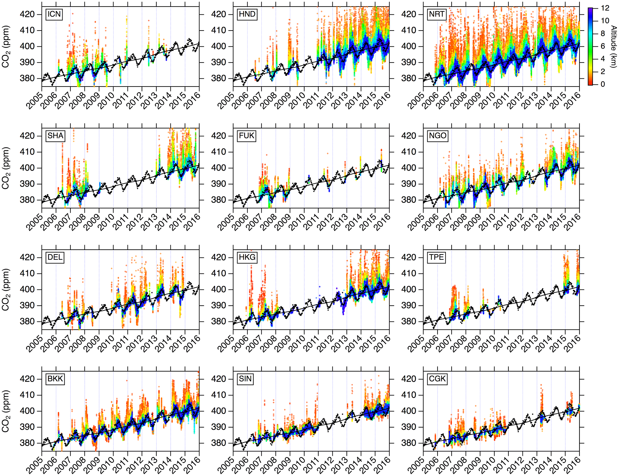
Figure 2Temporal variations in CO2 over various airports in Asia. See Table 1 and Fig. 1 for the airport codes. Individual CO2 data points are colored by altitude. The CO2 data over the two Shanghai airports (SHA and PVG) are merged and designated as SHA, and same for ICN (ICN and GMP) and TPE (TPE and TSA). Also shown in each panel for comparison are the flask-based CO2 data (black circles) and the long-term trend (black line) at the Mauna Loa Observatory (MLO; 19.54∘ N, 155.58∘ W; 3397 m above sea level; data obtained from the NOAA/ESRL/GMD).
2.3 Model simulation
To better understand processes that generate the observed tropospheric distribution of CO2 over the Asia-Pacific region, we analyze CO2 simulated by the model NICAM-TM (Nonhydrostatic Icosahedral Atmospheric Model-based Transport Model; Satoh et al., 2014). Details of the NICAM-TM CO2 simulation and the evaluation of its performance have been presented by Niwa et al. (2011, 2012). The atmospheric CO2 transport is calculated using the 6-hourly meteorological data nudged to the JRA-55 reanalysis. The horizontal model grid interval is about 240 km and the number of vertical model layers is 40. For CO2 simulation, fossil fuel (FF) emissions are obtained from the CDIAC (Carbon Dioxide Information Analysis Center) database (version 2013; Andres et al., 2013), while fire emissions are from the GFED (Global Fire Emission Database version 3.1; van der Werf et al., 2010). A priori terrestrial biospheric (BIO) fluxes are derived from the CASA (Carnegie-Ames-Stanford Approach) model (Randerson et al., 1997). The air–sea exchange is based on the JMA (Japan Meteorological Agency) ocean flux data (Iida et al., 2015). The BIO fluxes are optimized in the NICAM-TM model inversion by using the GLOBALVIEW data (http://www.esrl.noaa.gov/gmd/ccgg/globalview/, last access: January 2012) and the CONTRAIL data in the FT (Niwa et al., 2012). Thus, the simulated atmospheric CO2 is obtained from the optimized fluxes. We also examine simulated CO2 fields driven by two different emission fluxes: one by FF and the other by BIO (hereafter referred to as FF CO2 and BIO CO2, respectively). For comparison, the simulated data are sampled at times and locations coincident with the individual CONTRAIL CME data points, and processed in the same manner; stratospheric data are excluded by the model PV values; all CO2 data points are detrended by the MLO long-term trend in the model.

Figure 3(Left) Monthly climatological CO2 mole fraction (ΔCO2) in the UT over the Asia-Pacific region. The CO2 data taken at altitudes >8 km are averaged in each 5∘ × 5∘ bin. The CO2 data influenced by stratospheric air (PV >2 PVU) were excluded. Also shown are monthly averaged wind vectors at 250 hPa from the JCDAS/JRA-55 reanalysis data (averaged for the observation years). (Right) Histograms of ΔCO2 in each 5∘ latitude bands color coded in the same manner as in the left panels. Every histogram is normalized by maximum frequency.
3.1 Seasonal cycle of CO2 in the UT over the Asia-Pacific region
Figure 3 presents monthly averaged distributions of the UT ΔCO2 over the Asia-Pacific region (left panels) along with histograms in the respective 5∘ latitude bands (right panels). In the left panels, the black arrows indicate monthly averaged horizontal wind at 250 hPa pressure surface from the JCDAS reanalysis. We note that monthly CO2 distributions from the CONTRAIL data previously presented by Sawa et al. (2012) were calculated as averages in 20∘ (longitude) × 10∘ (latitude) bins. In this study we were able to increase the spatial resolution to 5∘ × 5∘ since we have more data. As seen in Fig. 3, the UT ΔCO2 undergoes a clear seasonal cycle that varies significantly with latitude and longitude.
In January–February, the UT ΔCO2 is relatively uniform in space (Fig. 3a and c), except in regions >35∘ N where the histograms show occurrences of higher ΔCO2 values (Fig. 3b and d). In March, high ΔCO2 values are apparent in regions >30∘ N over northern Japan and downwind (Fig. 3e), where a significantly increased frequency of high ΔCO2 up to 6 ppm is observed (Fig. 3f). This feature becomes more pronounced in April (Fig. 3h) with expanded areas of high ΔCO2 around Japan (Fig. 3g). By May, regions with high ΔCO2 extend to >20∘ N (Fig. 3i and j).
By June, the observed high ΔCO2 values over Japan and the northwestern Pacific nearly disappear (Fig. 3k). A significant fraction of the low ΔCO2 values down to −6 ppm and lower is observed at latitudes >35∘ N (Fig. 3l). Due to these low-CO2 values appearing at northern latitudes, the latitudinal gradient of UT ΔCO2 starts to reverse (i.e., northward positive to negative) after June, aided by moderately elevated CO2 observed at 15–30∘ N. In July, we begin to see very low ΔCO2 values below −6 ppm in high latitude regions (>40∘ N), particularly over boreal Eurasia (Fig. 3m and n). To the south, only very small spatial gradients are observed.
In August, we see the CO2 decrease broadly at all latitudes over the Asia-Pacific region, with distinctly low ΔCO2 values forming over South Asia to Southeast Asia (Fig. 3o). The UT wind field shows an anticyclonic wind circulation pattern over this region. This wind structure is coincident with the distinct low ΔCO2 observed over the continent, indicating that the low-CO2 air mass is confined within the UT anticyclone. This clear CO2 spatial structure associated with the anticyclone is for the first time depicted by the improved spatial resolution of the CONTRAIL data since Sawa et al. (2012). It is noted that such distinct low-CO2 structure does not appear until July, despite the fact that the anticyclonic wind pattern starts in June (Fig. 3k and m).
Moving into September, we see a further decrease in ΔCO2 across the wider Asia-Pacific region (Fig. 3q and r). The persistent UT anticyclonic structure is still observable in both ΔCO2 and wind fields, but the sharp boundary along the East Asian coast that was seen in August (i.e., longitudinal gradient or contrast between the continent and the ocean) is now to some degree blurred (see also Fig. 7a). In October, the anticyclonic low-ΔCO2 feature diminishes and ΔCO2 is now relatively uniform in the observation region. Thereafter ΔCO2 increases as a whole during the winter until the return of the spring.
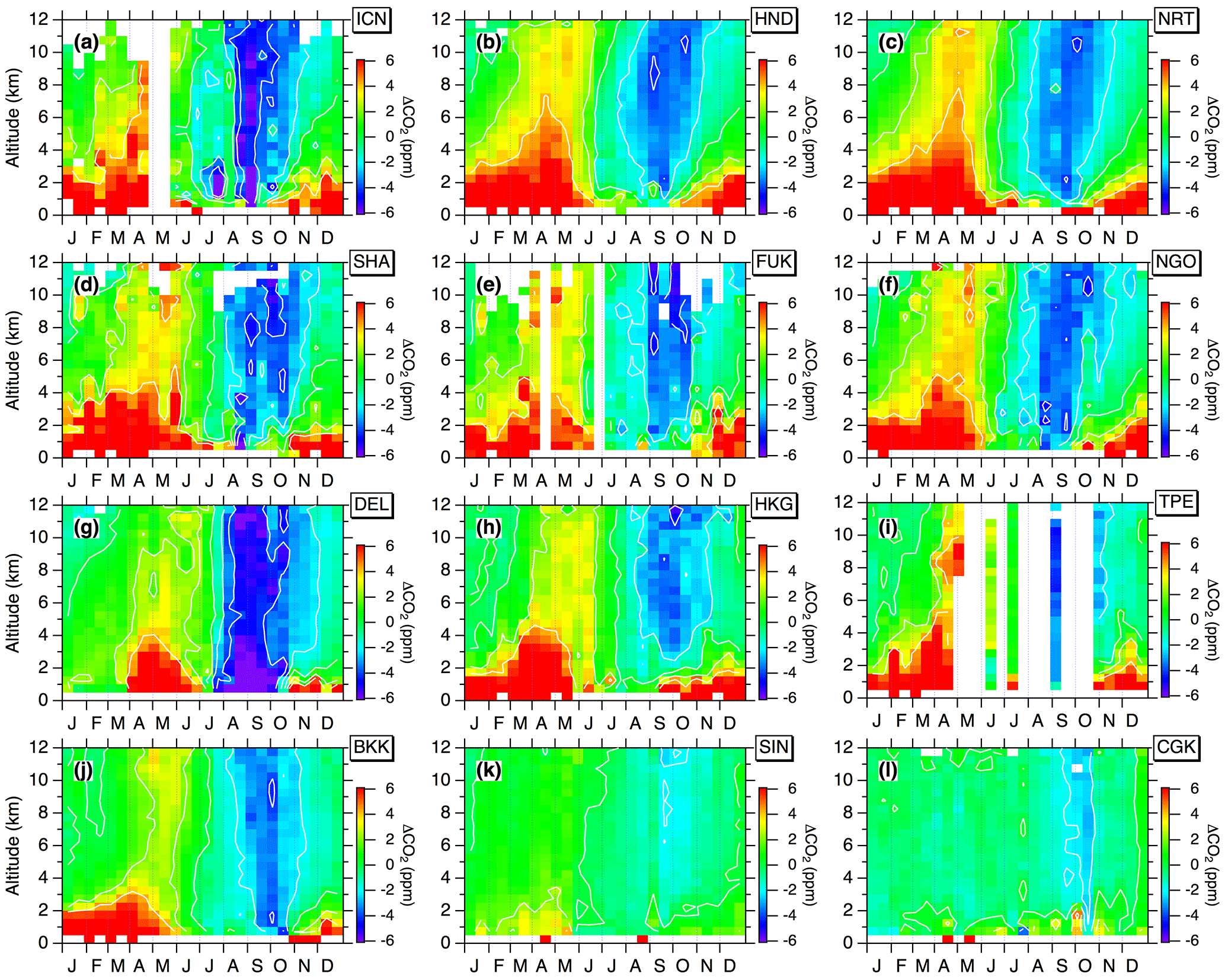
Figure 4Seasonal variations in vertical profiles of ΔCO2 over (a) ICN, (b) HND, (c) NRT, (d) SHA, (e) FUK, (f) NGO, (g) DEL, (h) HKG, (i) TPE, (j) BKK, (k) SIN, and (l) CGK. The airport codes are listed in Table 1. The CO2 data over some airports are merged, as described in Fig. 2. Vertical and horizontal bins are 500 m and 14-day intervals, respectively. White lines indicate isolines of ΔCO2.
3.2 Vertical gradients of CO2 over Asian cities
Figure 4 presents a climatology of seasonal variations and vertical profiles of ΔCO2 over 12 airports in Asia, as uniquely obtained by CONTRAIL observation. We consider these figures to represent large-scale (regional) features in the FT as a result of detrending and binning of the data (500 m altitude and 14-day averages from multiple-year data). At lower altitudes, relatively local features can be visible due to boundary layer (BL) processes and flight route biases near the airports, but examining such smaller-scale phenomena in detail is beyond the scope of this study. We also calculate for each airport, altitude variation in the standard deviation (SD) of ΔCO2 calculated for each 2-week and 500 m bin (Fig. 5), as an extended update of Shirai et al. (2012) who addressed synoptic-scale CO2 variability over NRT. This type of analysis is made possible due to CONTRAIL's high-frequency measurements during ascent/descent over the airports.
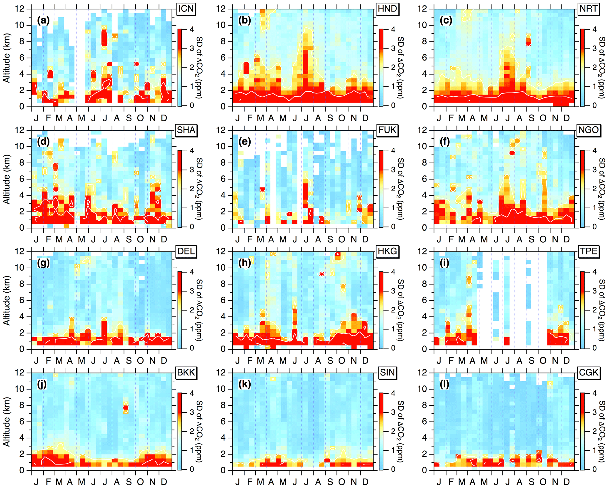
Figure 5Same as in Fig. 4 but for standard deviations of ΔCO2 in each bin. The standard deviation is calculated only when the bin has >5 data points.
Stephens et al. (2007) compiled CO2 data from flask-based aircraft observations at 12 sites around the world for comparison with model simulations. Flask CO2 data at 16 sites from the NOAA/ESRL aircraft program were reported by Sweeney et al. (2015), including some of the data analyzed by Stephens et al. (2007). The measurements by Sweeney et al. (2015) have revealed climatological CO2 variations over North America, whereas the present study focuses on Asia with more frequent in-flight observations. Since vertical profile measurements are relatively scarce over Asia (see supporting online material by Stephens et al., 2007), CONTRAIL observations provide greater spatiotemporal insight into regional carbon cycling processes. One of the remarkable features found in vertical CO2 profiles from other regions is the dramatic decrease in CO2 toward the ground in the summer period at mid-continental sites of the Northern Hemisphere (see Fig. S3 of Stephens et al., 2007 and Fig. 5 of Sweeney et al., 2015). Below we show that the vertical CO2 profiles and their seasonal changes observed by CONTRAIL in Asia are interestingly different from those reported by the previous measurements in other regions.
The seasonal CO2 cycles with spring maxima and summer minima, typical for the northern hemispheric troposphere (Stephens et al., 2007; Sweeney et al., 2015), are to some degree obvious across regions over the 12 airports (Fig. 4) in Asia. However, a clear difference from those outside Asia is the general absence of a dramatic decrease in CO2 near the ground in the summer. In other words, the contoured low ΔCO2 in the summer is apparently “floating” in the FT and not connected to the ground, implying that the observed vertical profiles in the summer are not dictated by overwhelming uptake underneath. This feature is observed at all airports except DEL. It is noteworthy that our measurement sites are all located in coastal areas except DEL, while previous measurements at inland sites generally showed more pronounced decreases of CO2 near the ground in the summer (Stephens et al., 2007; Sweeney et al., 2015). In contrast, the springtime maximum ΔCO2 extends from the ground to the UT, indicating that the surrounding or upwind regions of most airports are strong sources of CO2 during that season.
It is likely that some features shown in Fig. 4, especially in the BL, are due to the influence of nearby CO2 emissions. Indeed, at some airports, large elevations of CO2 values have been observed frequently in the BL. In order to reduce possible bias due to such pollution events, we did redraw Fig. 4 with median ΔCO2 values, instead of averaged values. We found no clear visual difference in the overall features discussed below. In fact, differences between average and median are mostly <1 ppm even below 2 km at all airports, except SHA and HKG where the value is ∼1.5 ppm on yearly average. Although pollution events are observed frequently over these two airports (as described below), we consider such “airport bias” in the climatological vertical profiles to be small within the scope of this study. Influence of nearby city emissions on the CONTRAIL observations will be addressed in our future publication.
NRT and HND, Japan, are the two airports over which the largest number of CO2 measurements have been collected by the CONTRAIL CME, giving relatively smooth climatology of ΔCO2 (Fig. 4b and c). Seasonal and vertical characteristics of CO2 over HND and NRT are quite similar to each other. In the FT, ΔCO2 reaches its seasonal maximum in the spring (April–May) and minimum in the late summer to early autumn (September–October), with the seasonal amplitude in general decreasing with altitude. We also find substantially enhanced SD below ∼2 km over HND and NRT in the winter (November–April) and summer (June–August) (Fig. 5b and c). The high summer variability propagates up to higher altitudes (∼6 km), presumably associated with enhanced vertical mixing in the summer. The vertical gradient in CO2 is small (<2 ppm) during the summer period (June–September), but a clear gradient is detectable for the rest of the year. These features are commonly observed over the other two Japanese airports Nagoya (NGO; ∼260 km west of Tokyo) and Fukuoka (FUK; ∼880 km west-southwest of Tokyo and ∼850 km east-northeast of Shanghai). Also notable is that, in September, CO2 decreases with altitude, this feature being observed widely over these four Japanese cities. ΔCO2 undergoes a seasonal cycle with spring maximum and summer minimum also over ICN (∼570 km northwest of FUK; Fig. 4a), but the minimum occurs in late August to early September, about a month earlier than observed over the aforementioned Japanese airports. The low ΔCO2 in the BL is a characteristic that is not observed over Japan.
Along the east coast of continental East Asia, measurements are obtained over three cities: SHA, HKG, and TPE (Fig. 4d, h, and i, respectively). ΔCO2 increases from September until May when it reaches a seasonal maximum. The seasonal minimum in the UT appears in September–October, lagging the lower troposphere (LT) minimum by about a month. We see remarkably high ΔCO2 values in the BL over SHA and HKG, these phenomena being particularly pronounced over SHA where we frequently observe ΔCO2 enhancements of >20 ppm below 1 km. The elevated ΔCO2 in the winter season (November–April) is also characterized by high variability (Fig. 5d and h). Although the seasonal and vertical characteristics of CO2 over TPE appear to be essentially similar to those over SHA and HKG; our measurements are sparse during May–October.
ΔCO2 over DEL shows a unique seasonal variation. We note that DEL is the only inland site, whereas the all other sites presented in this study are located near the coast. Prominent is the strong CO2 drawdown throughout the troposphere in August–September, with very little vertical gradient in the FT due to vigorous vertical mixing (Fig. 4g). Another interesting feature is the relatively low ΔCO2 in the BL ( km) during January–March. This wintertime CO2 stagnation over DEL was recently attributed to uptake by crops (mainly wheat) grown in the winter season in the surrounding region (Umezawa et al., 2016).
Clear seasonal CO2 variations are also visible over BKK (Fig. 4j). The seasonal maximum happens in March–April in the LT and propagates upward. These 2 months correspond to a period of enhanced ΔCO2 variability near the ground (Fig. 5j). Over SIN in Southeast Asia, ΔCO2 exhibits measurable seasonal variation (Fig. 4k). The seasonal variation in the FT over SIN is similar in phase with that observed over BKK, but with comparatively reduced magnitude. It should be also noted that, over SIN, the vertical gradient of ΔCO2 is small throughout the year. A maximum vertical ΔCO2 difference is only ∼2 ppm observed in the boreal spring. Lastly, for CGK in tropical Asia (Fig. 4l), the observed seasonality in ΔCO2 in the LT is hard to characterize due to relatively large variability. But interestingly, the seasonal phases are apparently different below and above 2.5 km. Below that height, relatively high ΔCO2 values appear during August–October, while, over the same period, ΔCO2 in the FT decreases until the October minimum.

Figure 6Comparison of the observed and simulated distributions of CO2 in the UT. Column 1 shows ΔCO2 observed by CONTRAIL CME. Columns 2–4 show ΔCO2, ΔFF CO2, and ΔBIO CO2 simulated by NICAM-TM. The CONTRAIL data are simply averaged for each grid, and the NICAM-TM data are sampled at locations and times corresponding to the observation data and analyzed in the same manner. Also shown are the simulated monthly distributions of CO2 at 250 hPa pressure surface in 2011 (column 5). Solid lines in white and black in column 5 indicate CO2 isolines and geopotential height at 250 hPa pressure surface, respectively.
3.3 Simulated CO2 distributions in the UT over the Asia-Pacific region
In Fig. 6, simulated (second column) monthly CO2 distributions in the UT are compared to the observations (first column). The model outputs are sampled at a location and time coincident with the observation and analyzed in the same manner as the measurements. The third and fourth column of panels show the simulated FF CO2 and BIO CO2, respectively. We do not present a contribution from biomass burning, since it is relatively minor (though not negligible) in evaluating the seasonal variation. Also shown are monthly CO2 distributions at 250 hPa pressure surface for 2011 (last column). We have chosen the model year 2011 as a representative year whose seasonal CO2 distribution patterns are not exceptional, although the simulated CO2 exhibits interannual variation due to year-by-year changes in meteorology and CO2 fluxes. Note that the model data in the last column are simple monthly averages at model resolutions; thus, both the UT and stratospheric model data are included and avoids sampling bias that might result from data availability as in the observations. However, the similarity in the features between the model and observed results, together with the model monthly averages, attests to the fact that the CME-based CO2 distribution is representative of the seasonal CO2 climatology in the UT.
By comparing with the observations, we see that NICAM-TM (second column) is able to reproduce the overall general seasonal features of the observed CO2 distribution pattern in the UT over the Asia-Pacific region. The model simulation (second column) shows seasonal CO2 elevations centered at 20–40∘ N in April–June, depletion of CO2 over boreal Eurasia starting from June, and a distinct decrease in CO2 over South Asia to Southeast Asia in August–September, all of which are in agreement with the observation (first column). In Sect. 4, we discuss how these features constitute the large-scale seasonal CO2 distributions, as depicted in the last column. One notable feature that is not well reproduced by the model is the high ΔCO2 values observed over northern Japan in April, the cause of which is yet to be determined.
4.1 Summertime CO2 drawdown
In Sect. 3.1, we presented two major features in the CO2 distribution in the UT over the Asia-Pacific region in the boreal summer: (1) the distinct low-CO2 values associated with the monsoon anticyclone over South Asia to Southeast Asia during August–September and (2) the highly variable low-CO2 values at northern latitudes (>40∘ N) during June–August (Fig. 3). These summertime low-CO2 phenomena are hereafter referred to as the “monsoon low CO2” and “boreal low CO2”, respectively.
4.1.1 Monsoon low CO2
In August, a distinct circular-shaped distribution of low CO2 over the Asian continent is prominent in both the observed and simulated ΔCO2 (Fig. 6u and v). The model reproduces the observation well in terms of the location of the spatially minimum CO2 (i.e., the low-CO2 over South Asia and northern Southeast Asia). Although the CONTRAIL data are not available over inland China (in particular over the Tibetan Plateau), the model simulation (Fig. 6y) offers a complete picture of the UT low-CO2 distribution associated with the monsoon anticyclone. Interestingly, the anticyclonic CO2 pattern is mainly composed of low BIO CO2 (Fig. 6x). The region of lowered CO2 in the monsoon anticyclone expands until September, as the confinement of the low CO2 in the anticyclone becomes less distinct than in August as a region-wide decrease in CO2 occurs (Fig. 6z, aa, and ad). The simulation indicates spreading of low BIO CO2 to the northwestern Pacific from the anticyclone. In October, the UT CO2 becomes nearly uniform again over the entire Asia-Pacific region (Fig. 6ae, af, and ai).
As described above, the monsoon low CO2 in the UT anticyclone is seasonally most distinct in August (Figs. 3 and 6), which is in fact coincident with the dynamical development of the summer monsoon anticyclone. Previous studies have shown that dynamical strengths of the monsoon anticyclone and convective activity reach their seasonal maxima in July–August (Randel and Park, 2006; Garny and Randel, 2013), and that, consequently, the confinement of the air mass within the UT anticyclone is seasonally strongest in August (Rauthe-Schöch et al., 2016). The CONTRAIL flights have only DEL where vertical profiles inside the monsoon low CO2 could be collected (see Fig. 3o). The DEL measurements clearly illustrate well-mixed CO2 in the FT with a pronounced decrease in the BL (Fig. 4g). This feature is consistent with the interpretation that the neighboring region of DEL (i.e., northwestern India) is part of the vertical conduit core that effectively transports surface flux signals upward to the upper tropospheric part of the summer monsoon anticyclone (Bergman et al., 2013). Our simulation shows that the BIO uptake in South Asia plays a dominant role in lowering the UT CO2 (Fig. 6). In this connection, model studies have demonstrated that aircraft data within the anticyclone have a significant impact in constraining surface CO2 fluxes in South Asia (Patra et al., 2011; Niwa et al., 2012). In August, over other Asian cities such as SIN, BKK, HKG, and SHA, the summertime ΔCO2 values are not as low as those in the monsoon anticyclone (Fig. 3o), which means that these cities are outside the monsoon vertical conduit.
In September, the vertical profiles over DEL (i.e., the core of the monsoon low CO2) retain vertically well-mixed low-CO2 mole fractions as in August (Fig. 4g). This is indicative of strong BIO CO2 uptake, as reflected in the optimized flux (see Fig. 5d of Niwa et al., 2012). At the same time, we see a region-wide CO2 decrease, as the August sharp CO2 gradient at the edge of the UT anticyclone becomes blurred (Fig. 3q). This implies a broad propagation of the monsoon low CO2 in the UT, as the anticyclonic confinement weakens (Garny and Randel, 2013; Rauthe-Schöch et al., 2016). The expansion of the monsoon low CO2 in the UT (Fig. 3q) is reflected in the vertical CO2 profiles over HKG and SHA where substantial CO2 decreases are observed in the UT in September (i.e., the vertical gradients of CO2 over both cities increase from August to September; see Fig. 4). A similar, but less pronounced, feature is observed further downwind over cities in Japan (FUK, NGO, NRT, and HND), as it is advected by strong westerly winds to the western Pacific in October. The decreasing CO2 with altitude in the late summer is unique over the Asia-Pacific region where outflow from the monsoon low CO2 in the UT is a significant contributing factor. The same process involving the Asian summer monsoon anticyclone can be invoked to explain the elevated methane (CH4) values of South Asian origin observed in the UT over the western Pacific in the summer (Umezawa et al., 2012). The high CH4 values in the Asian summer monsoon anticyclone, its formation mechanism, and outflow from the anticyclone were recently discussed by Chandra et al. (2017).
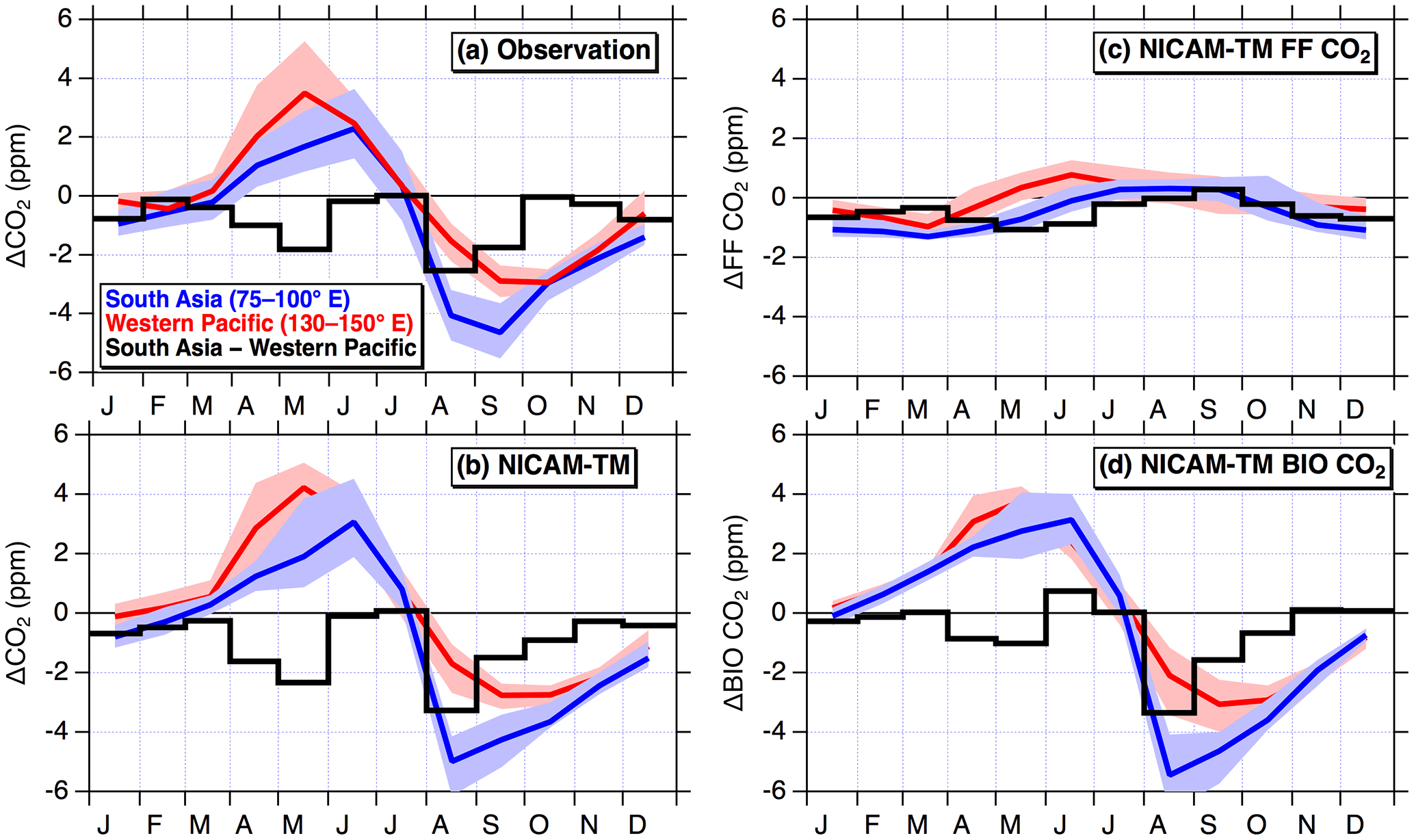
Figure 7(a) Seasonal variations in ΔCO2 in the UT over South Asia (blue; 20–30∘ N, 75–100∘ E) and western Pacific (red; 20–30∘ N, 130–150∘ E). Lines and shades are monthly medians, and 25th and 75th percentiles, respectively. Black solid line shows monthly difference of ΔCO2 between the two areas (South Asia – western Pacific, i.e., longitudinal gradient). (b) Same as in (a), but for the NICAM-TM simulated data. (c) Same as in (b), but for FF CO2 in the model. (d) Same as in (b), but for BIO CO2 in the model.
Figure 7a compares seasonal variations in ΔCO2 in the UT over the South Asian continent (75–100∘ E) and the western Pacific Ocean (130–150∘ E) at latitudes 20–30∘ N. Here we define longitudinal gradient as the difference in ΔCO2 between these two continental and oceanic areas (black line). The observed longitudinal gradient is nearly zero in July, increasing rapidly to 2.5 ppm in August, decreasing to 1.8 ppm in September, and then disappearing in October. This seasonal change is reproduced well by the NICAM-TM simulation (Fig. 7b). We also show a break down of the longitudinal gradient into BIO and FF CO2 contributions. Clearly, BIO CO2 is the predominant driver of the seasonal CO2 variation in the UT over both areas and contributes to the longitudinal gradient in August–September due to the monsoon anticyclone. Over South Asia, seasonal maximum contribution of BIO CO2 to the summertime decrease is seen in August. This effect is not observed until September over the western Pacific, a lag on the order of a month.
It is interesting to note the difference in the timing between the CO2 drawdown and the accumulation of other pollutants inside the UT monsoon anticyclone. As clearly seen in Fig. 3m, no enhancement/depletion in CO2 is observed in the UT monsoon anticyclone in July. This is in contrast to studies that have indicated an elevation of pollutant species within the monsoon anticyclone starting in June to July (e.g., Park et al., 2009; Xiong et al., 2009; Schuck et al., 2010; Randel et al., 2010). The difference between atmospheric CO2 and other pollutants lies in the fact that these “other pollutants” are mostly of anthropogenic origins that essentially have no seasonal cycle. The observed enhancement of these pollutants are therefore driven mostly by the anticyclone dynamics (Randel and Park, 2006; Park et al., 2009; Bergmann et al., 2013), and not by the seasonal variation in the surface emission, as in CO2. Therefore, the absence of the anticyclonic structure in CO2 in July is attributable to its surface flux characteristics. In July, the region's terrestrial biosphere might still be in transition from overwhelming respiration (net source) to photosynthesis (net sink) (Niwa et al., 2012; Patra et al., 2013), since substantial precipitation arrives 1–2 months after the onset of the monsoon (i.e., prevailing southwest wind) in June (India Meteorological Department at http://imd.gov.in/pages/monsoon_main.php, last access: 23 May 2018). From August to September, strong biospheric CO2 uptake in South Asia takes place (Niwa et al., 2012), giving rise to the observed monsoon low CO2 in the UT (Fig. 6) that is simulated well in our model.
4.1.2 Boreal low CO2
In July, a prominent feature that is common in the CONTRAIL measurements and the NICAM-TM simulation (Fig. 6p and q) is a sharp north–south CO2 gradient at 40–50∘ N, with low values to the north and relatively uniform CO2 to the south. In the NICAM-TM simulation, much of the BIO CO2 uptake in boreal Eurasia propagates to the Northern Pacific (Fig. 6s).
The boreal low CO2 (i.e., the deeper drawdown of CO2 and its earlier phase at higher latitudes) in the UT has been understood in the context of BIO CO2 uptake propagating from mid- to high latitudes (Tanaka et al., 1988; Nakazawa et al., 1991; Matsueda and Inoue, 1996; Matsueda et al., 2002). It is estimated that a substantial CO2 uptake by boreal biosphere starts in June and peaks in July to early August (e.g., Randerson et al., 1999; Saeki et al., 2013; Zhang et al., 2014), therefore the occurrence of the boreal low CO2 in the UT is consistent in phase with the atmospheric propagation of boreal BIO uptake. Sawa et al. (2012) showed that, in summer, convective uplift of surface low-CO2 air lowers CO2 in the FT at the Northern Hemisphere mid- to high latitudes. As clearly seen in Fig. 3, we observed the large CO2 variability (the wide spread of the histograms, see panels l, n, and p) in the UT north of 40∘ N in June–August. This large CO2 variability can be explained most likely by sporadic occurrences of convection over boreal Eurasia, as well as to a lesser extent by seasonally strongest and heterogeneous BIO CO2 uptake; such an example from the CONTRAIL measurement flights has been presented in Fig. 5 of Sawa et al. (2012). Miyazaki et al. (2008) pointed out that the boreal low CO2 in the summer is isolated from the lower latitudes due to slow mean meridional circulation and weak cyclonic activity during the season. This can be seen in the CONTRAIL data (Fig. 6p, see also Fig. 6 of Sawa et al., 2012) and the NICAM-TM simulation (Fig. 6q). It is also noted that the spread of the histogram over boreal Eurasia decreases in September (Fig. 3r), implying that the convective activity and BIO CO2 uptake over the continent seasonally weakens and the UT resumes “background” CO2 after the summer period of large fluctuations.
The extent to which the boreal low CO2 is advected has a significant impact on the observed seasonal cycles of CO2 in the LT over East Asian cities. As described earlier, the seasonal CO2 minimum over ICN occurs about a month earlier than over Japan at similar latitudes (Fig. 4). Based on the NICAM-TM model analysis of the ICN measurements (Niwa et al., 2017), it is found that air masses observed in the LT over ICN in the summer are influenced by surface fluxes in boreal Eurasia. As mentioned earlier, the boreal BIO CO2 uptake peaks in July, earlier than at midlatitudes. Accordingly, larger contributions of air masses from the north in the early summer would lower atmospheric CO2, shifting earlier the occurrence of the seasonal CO2 minimum at midlatitudes.
4.2 Seasonally elevated and highly variable CO2 in spring
We have shown in Sect. 3 that seasonally elevated CO2 is observed throughout the whole troposphere over the East Asia region in April–May (Figs. 3 and 4). This elevated CO2 is accompanied by an increased spread of ΔCO2 values in the UT north of 30∘ N in March–April (Fig. 3f and h). As shown by the NICAM-TM simulation, seasonally high CO2 can be explained mostly by the BIO emission fluxes, but a significant portion of the associated variability is due to enhanced synoptic-scale meteorological variability.
One of the most likely factors in meteorology is the active passage of eastward-tracking synoptic systems. In East Asia, cyclonic activity is most frequent in the spring (Chen et al., 1991; Adachi and Kimura, 2007). In association with the eastward moving springtime cyclonic activity, two major transport pathways have been suggested for pollutant outflow from the continental East Asia to different tropospheric layers over the northwestern Pacific. (1) The first mechanism involves the advection of polluted BL air behind the cyclonic cold front as it moves eastward over the East Asian continent out to the Pacific (Liu et al., 2003; Sawa et al., 2007). Consequently, periodic passages of cyclones produce episodic variations in anthropogenic trace gases in the BL across the northwestern Pacific (Liu et al., 1997; Liang et al., 2004; Sawa et al., 2007; Tohjima et al., 2010, 2014). (2) The second mechanism involves frontal uplift of air in front of a moving cold front, in what is called the warm conveyor belt. The uplift frequently takes place over south and central China and the plume travels northeastward along the warm conveyor belt to the northwestern Pacific (Bey et al., 2001; Liu et al., 2003; Miyazaki et al., 2003; Liang et al., 2004). Convective uplift along a frontal zone over central China and Southeast Asia also transports BL air to the FT (Miyazaki et al., 2003; Oshima et al., 2004). In addition to the above transport processes associated with cyclones, orographic forcing over south and central China has also been observed to uplift the BL air to the FT (Liu et al., 2003). Once in the FT, the plume can be easily exported to the Pacific by the midlatitude westerly winds (Bey et al., 2001; Liu et al., 2003).
In summary, periodic and episodic cyclonic uplifting of BL air over continental East Asia, with strong surface CO2 emissions, could explain the seasonal maximum level of CO2 and increased variability in the FT in the spring (Fig. 3). Using the CONTRAIL data, Shirai et al. (2012) also showed that the observed synoptic-scale variability in the FT CO2 over NRT increases in the spring, as air influenced by the continental East Asian CO2 emissions is advected towards Japan.
We have presented spatiotemporal variations in tropospheric CO2 over the Asia-Pacific region observed uniquely by the CONTRAIL commercial airliner measurements. High-frequency in-flight CO2 measurements by the CONTRAIL CME cover large parts of the Asia-Pacific region and contribute to an enhanced characterization and understanding of the climatological distribution of CO2 over the region. Some of the highlights in this study are summarized as follows.
In summer, the region-wide low CO2 across the Asia-Pacific region is primarily due to the CO2 drawdowns in two distinct regions: the monsoon low CO2 and the boreal low CO2. The monsoon low CO2 reflects South Asian biospheric CO2 uptake and its propagation in the UT in association with the development and decay of the Asian summer monsoon anticyclone. This process contributes significantly to the observed horizontal and vertical variations in CO2 over the Asia-Pacific region. The monsoon outflow increases in September as the anticyclone decays, delivering low CO2 (from the South Asian biosphere) to the UT over the northwestern Pacific. In contrast, the boreal low CO2 is driven by boreal terrestrial biospheric uptake. Heterogeneous spatial distributions of the biospheric flux, combined with the sporadic convective vertical transport over the Eurasian continent, cause seasonally large variability in the UT CO2 north of 40∘ N.
In spring, active passages of the eastward-tracking synoptic system sweep continental East Asia and transport the region's CO2 emissions up to the UT, elevating atmospheric CO2 over the northwestern Pacific. These synoptic systems also increase variability in CO2. Given the high-density CONTRAIL measurements over Asia, and in particular around Japan, the CONTRAIL data provide a promising opportunity for diagnosing detailed transport processes by midlatitude cyclones of CO2 emitted from continental East Asia.
The CONTRAIL commercial airliner measurements over the Asia-Pacific region can be exploited in constraining emissions of various trace gases from East Asia and South Asia, particularly in the context of the role of the Asian summer monsoon. Also, given the unique spatiotemporal measurements along the high-altitude cruise and vertical profiles, the CONTRAIL data can be used to evaluate emerging greenhouse gas data obtained by satellites.
The CONTRAIL CME data are available on the Global Environmental Database of the Center for Global Environmental Studies of NIES (https://doi.org/10.17595/20180208.001, last access: 7 October 2018). The data are also available from the ObsPack data product (http://www.esrl.noaa.gov/gmd/ccgg/obspack/, last access: 26 September 2018).
TU, HM and TM conceived and designed the study. TU performed the data analysis and wrote the paper. YS and TM ensured quality of the CONTRAIL CME CO2 data. YS formatted the JCDAS/JRA-55 reanalysis data for the data analysis. YN performed the NICAM-TM simulations and provided the model data. TM, HM, YS and LZ managed the project within the focus region of this study. All co-authors contributed to the text.
The authors declare that they have no conflict of interest.
This article is part of the special issue “The 10th International Carbon Dioxide Conference (ICDC10) and the 19th WMO/IAEA Meeting on Carbon Dioxide, other Greenhouse Gases and Related Measurement Techniques (GGMT-2017) (AMT/ACP/BG/CP/ESD inter-journal SI)”. It is a result of the 10th International Carbon Dioxide Conference, Interlaken, Switzerland, 21–25 August 2017.
We are grateful to engineers and staff of the Japan Airlines, JAL
Foundation, and JAMCO Tokyo for supporting the CONTRAIL project. We also
thank Keiichi Katsumata, Hisayo Sandanbata, and Eri Matsuura (NIES) for
technical support. We thank Ed Dlugokencky for the NOAA's flask-based
CO2 data at Mauna Loa. We acknowledge efforts by NICAM developers of
Atmosphere and Ocean Research Institute of the University of Tokyo, Japan
Agency for Marine-Earth Science and Technology, and RIKEN. We thank Kaz
Higuchi (York University, Canada) for his comments to improve the
manuscript. We also thank two anonymous referees for helpful comments. The
CONTRAIL observation was financially supported by the research fund by
Global Environmental Research Coordination System and by Environment
Research and Technology Development Funds (2-1401 and 2-1701) from the Ministry
of the Environment, Japan, and the Environmental Restoration and Conservation
Agency.
Edited by: Rachel Law
Reviewed by: two anonymous referees
Adachi, S. and Kimura, F.: A 36-year Climatology of Surface Cyclogenesis in East Asia Using High-resolution Reanalysis Data, SOLA, 3, 113–116, https://doi.org/10.2151/sola.2007?029, 2007.
Andres, R. J., Boden, T. A., and Marland, G.: Monthly Fossil-Fuel CO2 Emissions: Mass of Emissions Gridded by One Degree Latitude by One Degree Longitude, Carbon Dioxide Information Analysis Center, Oak Ridge National Laboratory, U. S. Department of Energy, Oak Ridge, Tenn., USA, https://doi.org/10.3334/CDIAC/ffe.MonthlyMass.2013, 2013.
Ballantyne, A. P., Alden, C. B., Miller, J. B., Tans P. P., and White, J. W. C.: Increase in observed net carbon dioxide uptake by land and oceans during the past 50 years, Nature, 488, 70–72, https://doi.org/10.1038/nature11299, 2012.
Bergman, J. W., Fierli, F., Jensen, E. J., Honomichl, S., and Pan, L. L.: Boundary layer sources for the Asian anticyclone: Regional contributions to a vertical conduit, J. Geophys. Res.-Atmos., 118, 2560–2575, https://doi.org/10.1002/jgrd.50142, 2013.
Bey, I., Jacob, D. J., Logan, J. A., and Yantosca, R. M.: Asian chemical outflow to the Pacific in spring: Origins, pathways, and budgets, J. Geophys. Res., 106, 23097–23113, https://doi.org/10.1029/2001JD000806, 2001.
Boden, T. A., Marland, G., and Andres, R. J.: Global, Regional, and National Fossil-Fuel CO2 Emissions. Carbon Dioxide Information Analysis Center, Oak Ridge National Laboratory, U.S. Department of Energy, Oak Ridge, Tenn., USA, https://doi.org/10.3334/CDIAC/00001 V2016, 2016.
Brenninkmeijer, C. A. M., Crutzen, P., Boumard, F., Dauer, T., Dix, B., Ebinghaus, R., Filippi, D., Fischer, H., Franke, H., Frieß, U., Heintzenberg, J., Helleis, F., Hermann, M., Kock, H. H., Koeppel, C., Lelieveld, J., Leuenberger, M., Martinsson, B. G., Miemczyk, S., Moret, H. P., Nguyen, H. N., Nyfeler, P., Oram, D., O'Sullivan, D., Penkett, S., Platt, U., Pupek, M., Ramonet, M., Randa, B., Reichelt, M., Rhee, T. S., Rohwer, J., Rosenfeld, K., Scharffe, D., Schlager, H., Schumann, U., Slemr, F., Sprung, D., Stock, P., Thaler, R., Valentino, F., van Velthoven, P., Waibel, A., Wandel, A., Waschitschek, K., Wiedensohler, A., Xueref-Remy, I., Zahn, A., Zech, U., and Ziereis, H.: Civil Aircraft for the regular investigation of the atmosphere based on an instrumented container: The new CARIBIC system, Atmos. Chem. Phys., 7, 4953–4976, https://doi.org/10.5194/acp-7-4953-2007, 2007.
Calle, L., Canadell, J. G., Patra, P., Ciais, P., Ichii, K., Tian, H., Kondo, M., Piao, S., Arneth, A., Harper, A. B., Ito, A., Kato, E., Koven, C., Sitch, S., Stocker, B. D., Vivoy, N., Wiltshire, A., Zaehle, S., and Poulter, B.: Regional carbon fluxes from land use and land cover change in Asia, 1980–2009, Environ. Res. Lett., 11, 074011, https://doi.org/10.1088/1748-9326/11/7/074011, 2016.
Cervarich, M., Shu, S., Jain, A. K., Arneth, A., Canadell, J., Friedlingstein, P., Houghton, R. A., Kato, E., Koven, C., Patra, P., Poulter, B., Sitch, S., Stocker, B., Viovy, N., Wiltshire, A., and Zeng, N.: The terrestrial carbon budget of South and Southeast Asia, Environ. Res. Lett., 11, 105006, https://doi.org/10.1088/1748-9326/11/10/105006, 2016.
Chandra, N., Hayashida, S., Saeki, T., and Patra, P. K.: What controls the seasonal cycle of columnar methane observed by GOSAT over different regions in India?, Atmos. Chem. Phys., 17, 12633–12643, https://doi.org/10.5194/acp-17-12633-2017, 2017.
Chen, S.-J., Kuo, Y.-H., Zhang, P.-Z., and Bai, Q.-F.: Synoptic climatology of cyclogenesis over East Asia, 1958–1987, Mon. Weather Rev., 119, 1407–1418, https://doi.org/10.1175/1520-0493(1991)119<1407:SCOCOE>2.0.CO;2, 1991.
Garny, H. and Randel, W. J.: Dynamic variability of the Asian monsoon anticyclone observed in potential vorticity and correlations with tracer distributions, J. Geophys. Res.-Atmos., 118, 13421–13433, https://doi.org/10.1002/2013JD020908, 2013.
Gurney, K. R., Law, R. M., Denning, A. S., Rayner, P. J., Baker, D., Bousquet, P., Bruhwiler, L., Chen, Y.-H., Ciais, P., Fan, S., Fung, I. Y., Gloor, M., Heimann, M., Higuchi, K., John, J., Maki, T., Maksyutov, S., Masarie, K., Peylin, P., Prather, M., Pak, B. C., Randerson, J., Sarmiento, J., Taguchi, S., Takahashi, T., and Yuen, C.-W.: Towards robust regional estimates of CO2 sources and sinks using atmospheric transport models, Nature, 415, 626–630, https://doi.org/10.1038/415626a, 2002.
Hoor, P., Fischer, H., Lange, L., Lelieveld, J., and Brunner, D.: Seasonal variations of a mixing layer in the lowermost stratosphere as identified by the CO-O3 correlation from in situ measurements, J. Geophys. Res., 107, 4044, https://doi.org/10.1029/2000JD000289, 2002.
Iida Y., Kojima, A., Takatani, Y., Nakano T., Midorikawa, T., and Ishii, M.: Trends in pCO2 and sea-air CO2 flux over the global open oceans for the last two decades, J. Oceanogr., 71, 637–661, https://doi.org/10.1007/s10872-015-0306-4, 2015.
Jiang, F., Wang, H. M., Cheu, J. M., Machida, T., Zhou, L. X., Ju, W. M., Matsueda, H., and Sawa, Y.: Carbon balance of China constrained by CONTRAIL aircraft CO2 measurements, Atmos. Chem. Phys., 14, 10133–10144, https://doi.org/10.5194/acp-14-10133-2014, 2014.
Jiang, F., Chen, J. M., Zhou, L., Ju, W., Zhang, H., Machida, T., Ciais, P., Peters, W., Wang, H., Chen, B., Liu, L., Zhang, C., Matsueda, H., and Sawa, Y.: A comprehensive estimate of recent carbon sinks in China using both top-down and bottom-up approaches, Sci. Rep., 6, 22130, https://doi.org/10.1038/srep22130, 2016.
Kobayashi, S., Ota, Y., Harada, Y., Ebita, A., Moriya, M., Onoda, H., Onogi, K., Kamahori, H., Kobayashi, C., Endo, H., Miyaoka, K., and Takahashi, K.: The JRA-55 reanalysis: general specifications and basic characteristics, J. Meteorol. Soc. Jpn., 93, 1, 5–48, https://doi.org/10.2151/jmsj.2015-001, 2015.
Lawrence, M. G. and Lelieveld, J.: Atmospheric pollutant outflow from southern Asia: a review, Atmos. Chem. Phys., 10, 11017–11096, https://doi.org/10.5194/acp-10-11017-2010, 2010.
Liang, Q., Jaeglé, L., Jaffe, D. A., Weiss-Penzias, P., Heckman, A., and Snow, J. A.: Long-range transport of Asian pollution to the northeast Pacific: Seasonal variations and transport pathways of carbon monoxide, J. Geophys. Res., 109, D23S07, https://doi.org/10.1029/2003JD004402, 2004.
Liu, C.-M., Buhr, M., and Merrill, J. T.: Ground-based observation of ozone, carbon monoxide, and sulfur dioxide at Kenting, Taiwan, during the PEM-West B campaign, J. Geophys. Res., 102, 28613–28625, https://doi.org/10.1029/96JD02980, 1997.
Liu, H., Jacob, D. J., Bey, I., Yantosca, R. M., Duncan, B. N., and Sachse, G. W.: Transport pathways for Asian pollution outflow over the Pacific: Interannual and seasonal variations, J. Geophys. Res., 108, 8786, https://doi.org/10.1029/2002JD003102, 2003.
Machida, T., Matsueda, H., Sawa, Y., Nakagawa, Y., Hirotani, K., Kondo, N., Goto, K., Ishikawa, K., Nakazawa, T., and Ogawa, T.: Worldwide measurements of atmospheric CO2 and other trace gas species using commercial airlines, J. Atmos. Oceanic Technol., 25, 1744–1754, https://doi.org/10.1175/2008JTECHA1082.1, 2008.
Machida, T., Sawa, Y., Matsueda, H., and Niwa, Y.: Atmospheric CO2 mole fraction data of CONTRAIL-CME, https://doi.org/10.17595/20180208.001, 2018.
Matsueda, H. and Inoue, H. Y.: Measurements of atmospheric CO2 and CH4 using a commercial airliner from 1993 to 1994, Atmos. Environ., 30, 10–11, 1647–1655, https://doi.org/10.1016/1352-2310(95)00374-6, 1996.
Matsueda, H., Inoue, H. Y., and Ishii M.: Aircraft observation of carbon dioxide at 8–13 km altitude over the western Pacific from 1993 to 1999, Tellus, 54B, 1–21, https://doi.org/10.1034/j.1600-0889.2002.00304.x, 2002.
Miyazaki, K., Patra, P. K., Takigawa, M., Iwasaki, T., and Nakazawa, T.: Global-scale transport of carbon dioxide in the troposphere, J. Geophys. Res., 113, D15301, https://doi.org/10.1029/2007JD009557, 2008.
Miyazaki, Y., Kondo, Y., Koike, M., Fuelberg, H. E., Kiley, C. M., Kita, K., Takegawa, N., Sachse, G. W., Flocke, F., Weinheimer, A. J., Singh, H. B., Eisele, F. L., Zondlo, M., Talbot, R. W., Sandholm, S. T., Avery, M. A., and Blake, D. R.: Synoptic-scale transport of reactive nitrogen over the western Pacific in spring, J. Geophys. Res., 108, 8788, https://doi.org/10.1029/2002JD003248, 2003.
Nakazawa, T., Miyashita, K., Aoki, S., and Tanaka, M.: Temporal and spatial variations of upper tropospheric and lower stratospheric carbon dioxide, Tellus, 43B, 106–117, https://doi.org/10.1034/j.1600-0889.1991.t01-1-00005.x, 1991.
Nakazawa, T., Ishizawa, M., Higuchi, K., and Trivett, N. B. A.: Two curve fitting methods applied to CO2 flask data, Environmetrics, 8, 197–218, https://doi.org/10.1002/(SICI)1099-095X(199705)8:3<197::AID-ENV248>3.0.CO;2-C, 1997.
Niwa, Y., Patra, P. K., Sawa, Y., Machida, T., Matsueda, H., Belikov, D., Maki, T., Ikegami, M., Imasu, R., Maksyutov, S., Oda, T., Satoh, M., and Takigawa, M.: Three-dimensional variations of atmospheric CO2: aircraft measurements and multi-transport model simulations, Atmos. Chem. Phys., 11, 13359–13375, https://doi.org/10.5194/acp-11-13359-2011, 2011.
Niwa, Y., Machida, T., Sawa, Y., Matsueda, H., Schuck, T. J., Brenninkmeijer, C. A. M., Imasu, R., and Satoh, M.: Imposing strong constraints on tropical terrestrial CO2 fluxes using passenger aircraft based measurements, J. Geophys. Res., 117, D11303, https://doi.org/10.1029/2012JD017474, 2012.
Niwa, Y., Tomita, H., Satoh, M., Imasu, R., Sawa, Y., Tsuboi, K., Matsueda, H., Machida, T., Sasakawa, M., Belan, B., and Saigusa, N.: A 4D-Var inversion system based on the icosahedral grid model (NICAM-TM 4D-Var v1.0) – Part 1: Offline forward and adjoint transport models, Geosci. Model Dev., 10, 1157–1174, https://doi.org/10.5194/gmd-10-1157-2017, 2017.
Onogi, K., Tsutsui, J., Koide, H., Sakamoto, M., Kobayashi, S., Hatsushika, H., Matsumoto, T., Yamazaki, N., Kamahori, H., Takahashi, K., Kadokura, S., Wada, K., Kato, K., Oyama, R., Ose, T., Mannoji, N., and Taira, R.: The JRA-25 Reanalysis, J. Meteorol. Soc. Jpn., 85, 369–432, https://doi.org/10.2151/jmsj.85.369, 2007.
Oshima, N., Koike, M., Nakamura, H., Kondo, Y., Takegawa, N., Miyazaki, Y., Blake, D. R., Shirai, T., Kita, K., Kawakami, S., and Ogawa, T.: Asian chemical outflow to the Pacific in late spring observed during the PEACE-B aircraft mission, J. Geophys. Res., 109, D23S05, https://doi.org/10.1029/2004JD004976, 2004.
Park, M., Randel, W. J., Emmons, L. K., and Liversey, N. J.: Transport pathways of carbon monoxide in the Asian summer monsoon diagnosed from MOZART, J. Geophys. Res., 114, D08303, https://doi.org/10.1029/2008JD010621, 2009.
Patra, P. K., Law, R. M., Peters, W., Rödenbeck, C., Takigawa, M., Aulagnier, C., Baker, I., Bergmann, D. J., Bousquet, P., Brandt, J., Bruhwiler, L., Cameron-Smith, P. J., Christensen, J. H., Delage, F., Denning, A. S., Fan, S., Geels, C., Houweling, S., Imasu, R., Karstens, U., Kawa, S. R., Kleist, J., Krol, M. C., Lin, S.-J., Lokupitiya, R., Maki, T., Maksyutov, S., Niwa, Y., Onishi, R., Parazoo, N., Pieterse, G., Rivier, L., Satoh, M., Serrar, S., Taguchi, S., Vautard, R., Vermeulen, A. T., and Zhu, Z.: TransCom model simulations of hourly atmospheric CO2: Analysis of synoptic-scale variations for the period 2002–2003, Global Biogeochem. Cy., 22, GB4013, https://doi.org/10.1029/2007GB003081, 2008.
Patra, P. K., Niwa, Y., Schuck, T. J., Brenninkmeijer, C. A. M., Machida, T., Matsueda, H., and Sawa, Y.: Carbon balance of South Asia constrained by passenger aircraft CO2 measurements, Atmos. Chem. Phys., 11, 4163–4175, https://doi.org/10.5194/acp-11-4163-2011, 2011, 2011.
Patra, P. K., Canadell, J. G., Houghton, R. A., Piao, S. L., Oh, N.-H., Ciais, P., Manjunath, K. R., Chhabra, A., Wang, T., Bhattacharya, T., Bousquet, P., Hartman, J., Ito, A., Mayorga, E., Niwa, Y., Raymond, P. A., Sarma, V. V. S. S., and Lasco, R.: The carbon budget of South Asia, Biogeosciences, 10, 513–527, https://doi.org/10.5194/bg-10-513-2013, 2013.
Randel, W. J. and Park, M.: Deep convective influence on the Asian summer monsoon anticyclone and associated tracer variability observed with Atmospheric Infrared Sounder (AIRS), J. Geophys. Res., 111, D12314, https://doi.org/10.1029/2005JD006490, 2006.
Randel, W. J., Park, M., Emmons, L., Kinnison, D., Bernath, P., Walker, K. A., Boone, C., and Pumphrey, H.: Asian Monsoon Transport of Pollution to the Stratosphere, Science, 328, 611–613, https://doi.org/10.1126/science.1182274, 2010.
Randerson, J. T., Thompson, M. V., Conway, T. J., Fung, I. Y., and Field, C. B.: The contribution of terrestrial sources and sinks to trends in the seasonal cycle of atmospheric carbon dioxide, Global Biogeochem. Cy., 11, 535–560, https://doi.org/10.1029/97GB02268, 1997.
Randerson, J. T., Field, C. B., Fung, I. Y., and Tans, P. P.: Increases in early season ecosystem uptake explain recent changes in the seasonal cycle of atmospheric CO2 at high northern latitudes, Geophys. Res. Lett., 26, 2765–2768, https://doi.org/10.1029/1999GL900500, 1999.
Rauthe-Schöch, A., Baker, A. K., Schuck, T. J., Brenninkmeijer, C. A. M., Zahn, A., Hermann, M., Stratmann, G., Ziereis, H., van Velthoven, P. F. J., and Lelieveld, J.: Trapping, chemistry, and export of trace gases in the South Asian summer monsoon observed during CARIBIC flights in 2008, Atmos. Chem. Phys., 16, 3609–3629, https://doi.org/10.5194/acp-16-3609-2016, 2016.
Saeki, T., Maksyutov, S., Sasakawa, M., Machida, T., Arshinov, M., Tans, P., Conway, T. J., Saito, M., Valsala, V., Oda, T., Andres, R. J., and Belikov, D.: Carbon flux estimation for Siberia by inverse modeling constrained by aircraft and tower CO2 measurements, J. Geophys. Res.-Atmos., 118, 1100–1122, https://doi.org/10.1002/jgrd.50127, 2013.
Satoh, M., Tomita, H., Yashiro, H., Miura, H., Kodama, C., Seiki, T., Noda, A. T., Yamada, Y., Goto, D., Sawada, M., Miyoshi, T., Niwa, Y., Hara, M., Ohno, T., Iga, S., Arakawa, T., Inoue, T., and Kubokawa, H.: The Non-hydrostatic Icosahedral Atmospheric Model: description and development, Prog. Earth Planet. Sci., 1, 1–32, https://doi.org/10.1186/s40645-014-0018-1, 2014.
Sawa, Y., Matsueda, H., Makino, Y., Inoue, H. Y., Murayama, S., Hirota, M., Tsutsumi, Y., Zaizen, Y., Ikegami, M., and Okada, K.: Aircraft Observation of CO2, CO, O3 and H2 over the North Pacific during the PACE-7 Campaign, Tellus, 56B, 2–20, https://doi.org/10.1111/j.1600-0889.2004.00088.x, 2004.
Sawa, Y., Tanimoto, H., Yonemura, S., Matsueda, H., Wada, A., Taguchi, S., Hayasaka, T., Tsuruta, H., Tohjima, Y., Mukai, H., Kikuchi, N., Katagiri, S., and Tsuboi, K.: Widespread pollution events of carbon monoxide observed over the western North Pacific during the East Asian Regional Experiment (EAREX) 2005 campaign, J. Geophys. Res., 112, D22S26, https://doi.org/10.1029/2006JD008055, 2007.
Sawa, Y., Machida, T., and Matsueda, H.: Seasonal variations of CO2 near the tropopause observed by commercial aircraft, J. Geophys. Res., 113, D23301, https://doi.org/10.1029/2008JD010568, 2008.
Sawa, Y., Machida, T., and Matsueda, H.: Aircraft observation of the seasonal variation in the transport of CO2 in the upper atmosphere, J. Geophys. Res., 117, D05305, https://doi.org/10.1029/2011JD016933, 2012.
Sawa, Y., Machida, T., Matsueda, H., Niwa, Y., Tsuboi, K., Murayama, S., Morimoto, S., and Aoki, S.: Seasonal changes of CO2, CH4, N2O, and SF6 in the upper troposphere/lower stratosphere over the Eurasian continent observed by commercial airliner, Geophys. Res. Lett., 42, 2001–2008, https://doi.org/10.1002/2014GL062734, 2015.
Schuck, T. J., Brenninkmeijer, C. A. M., Baker, A. K., Slemr, F., van Velthoven, P. F. J., and Zahn, A.: Greenhouse gas relationships in the Indian summer monsoon plume measured by the CARIBIC passenger aircraft, Atmos. Chem. Phys., 10, 3965–3984, https://doi.org/10.5194/acp-10-3965-2010, 2010.
Shirai, T., Machida, T., Marsueda, H., Sawa, Y., Niwa, Y., Maksyutov, S., and Higuchi, K.: Relative contribution of transport/surface flux to the seasonal vertical synoptic CO2 variability in the troposphere over Narita, Tellus, 64B, 19138, https://doi.org/10.3402/tellusb.v64i0.19138, 2012.
Shirai, T., Ishizawa, M., Zhuravlev, R., Ganshin, A., Belikov, D., Saito, M., Oda, T., Valsala, V., Gomez-Pelaez, A. J., Langenfelds, R., and Maksyutov, S.: A decadal inversion of CO2 using the Global Eulerian–Lagrangian Coupled Atmospheric model (GELCA): sensitivity to the ground-based observation network, Tellus B, 69, 1291158, https://doi.org/10.1080/16000889.2017.1291158, 2017.
Stephens, B. B., Gurney, K. R., Tans, P. P., Sweeney, C., Peters, W., Bruhwiler, L., Ciais, P., Ramonet, M., Bousquet, P., Nakazawa, T., Aoki, S., Machida, T., Inoue, G., Vinnichenko, N., Lloyd, J., Jordan, A., Heimann, M., Shibistova, O., Langenfelds, R. L., Steele, L. P., Francey, R. J., and Denning, A. S.: Weak northern and strong tropical land carbon uptake from vertical profiles of atmospheric CO2, Science, 316, 1732–1735, doi:10.1126/science.1137004, 2007.
Sweeney, C., Karion, A., Wolter, S., Newberger, T., Guenther, D., Higgs, J. A., Andrews, A. E., Lang, P. M., Neff, D., Dlugokencky, E., Miller, J. B., Montzka, S. A., Miller, B. R., Masarie, K. A., Biraud, S. C., Novelli, P. C., Crotwell, M., Crotwell, A. M., Thoning, K., and Tans, P. P.: Seasonal climatology of CO2 across North America from aircraft measurements in the NOAA/ESRL Global Greenhouse Gas Reference Network, J. Geophys. Res.-Atmos., 120, 5155–5190, https://doi.org/10.1002/2014JD022591, 2015.
Tanaka, M., Nakazawa, T., Aoki, S., and Ohshima, H.: Aircraft measurements of tropospheric carbon dioxide over the Japanese islands, Tellus, 40B, 16–22, https://doi.org/10.1111/j.1600-0889.1988.tb00209.x, 1988.
Tohjima, Y., Mukai, H., Hashimoto, S., and Patra, P. K.: Increasing synoptic scale variability in atmospheric CO2 at Hateruma Island associated with increasing East-Asian emissions, Atmos. Chem. Phys., 10, 453–462, https://doi.org/10.5194/acp-10-453-2010, 2010.
Tohjima, Y., Kubo, M., Minejima, C., Mukai, H., Tanimoto, H., Ganshin, A., Maksyutov, S., Katsumata, K., Machida, T., and Kita, K.: Temporal changes in the emissions of CH4 and CO from China estimated from CH4∕CO2 and CO/CO2 correlations observed at Hateruma Island, Atmos. Chem. Phys., 14, 1663–1677, https://doi.org/10.5194/acp-14-1663-2014, 2014.
Umezawa, T., Machida, T., Ishijima, K., Matsueda, H., Sawa, Y., Patra, P. K., Aoki, S., and Nakazawa, T.: Carbon and hydrogen isotopic ratios of atmospheric methane in the upper troposphere over the Western Pacific, Atmos. Chem. Phys., 12, 8095–8113, https://doi.org/10.5194/acp-12-8095-2012, 2012.
Umezawa, T., Niwa, Y., Sawa, Y., Machida, T., and Matsueda, H.: Winter crop CO2 uptake inferred from CONTRAIL measurements over Delhi, India, Geophys. Res. Lett., 43, 11859–11866, https://doi.org/10.1002/2016GL070939, 2016.
van der Werf, G. R., Randerson, J. T., Giglio, L., Collatz, G. J., Mu, M., Kasibhatla, P. S., Morton, D. C., DeFries, R. S., Jin, Y., and van Leeuwen, T. T.: Global fire emissions and the contribution of deforestation, savanna, forest, agricultural, and peat fires (1997–2009), Atmos. Chem. Phys., 10, 11707–11735, https://doi.org/10.5194/acp-10-11707-2010, 2010.
Xiong, X., Houweling, S., Wei, J., Maddy, E., Sun, F., and Barnet, C.: Methane plume over south Asia during the monsoon season: satellite observation and model simulation, Atmos. Chem. Phys., 9, 783–794, https://doi.org/10.5194/acp-9-783-2009, 2009.
Zhang, H. F., Chen, B. Z., van der Laan-Luijk, I. T., Machida, T., Matsueda, H., Sawa, Y., Fukuyama, Y., Langenfelds, R., van der Schoot, M., Xu, G., Yan, J. W., Cheng, M. L., Zhou, L. X., Tans, P. P., and Peters, W.: Estimating Asian terrestrial carbon fluxes from CONTRAIL aircraft and surface CO2 observations for the period 2006–2010, Atmos. Chem. Phys., 14, 5807–5824, https://doi.org/10.5194/acp-14-5807-2014, 2014.