Cloud vertical structure over a tropical station obtained using long-term high-resolution radiosonde measurements

Cloud vertical structure, including top and base altitudes, thickness of cloud layers, and the vertical distribution of multilayer clouds, affects large-scale atmosphere circulation by altering gradients in the total diabatic heating and cooling and latent heat release. In this study, long-term (11 years) observations of high-vertical-resolution radiosondes are used to obtain the cloud vertical structure over a tropical station at Gadanki (13.5^∘ N, 79.2^∘ E), India. The detected cloud layers are verified with independent observations using cloud particle sensor (CPS) sonde launched from the same station. High-level clouds account for 69.05 %, 58.49 %, 55.5 %, and 58.6 % of all clouds during the pre-monsoon, monsoon, post-monsoon, and winter seasons, respectively. The average cloud base (cloud top) altitudes for low-level, middle-level, high-level, and deep convective clouds are 1.74 km (3.16 km), 3.59 km (5.55 km), 8.79 km (10.49 km), and 1.22 km (11.45 km), respectively. Single-layer, two-layer, and three-layer clouds account for 40.80 %, 30.71 %, and 19.68 % of all cloud configurations, respectively. Multilayer clouds occurred more frequently during the monsoon with 34.58 %. Maximum cloud top altitude and cloud thickness occurred during the monsoon season for single-layer clouds and the uppermost layer of multiple-layer cloud configurations. In multilayer cloud configurations, diurnal variations in the thickness of upper-layer clouds are larger than those of lower-layer clouds. Heating and cooling in the troposphere and lower stratosphere due to these cloud layers are also investigated and peak cooling (peak warming) is found below (above) the cold-point tropopause (CPT) altitude. The magnitude of cooling (warming) increases from single-layer to four- or more-layer cloud occurrence. Further, the vertical structure of clouds is also studied with respect to the arrival date of the Indian summer monsoon over Gadanki.

1 Introduction

Clouds are vital in driving the climate system as they play an important role in radiation budget, general circulation, and the hydrological cycle (Ramanathan et al., 1989; Rossow and Lacis, 1990; Wielicki et al., 1995; Li et al., 1995; Stephens, 2005; Yang et al., 2010; Huang, 2013). By interacting with both shortwave and longwave radiation, clouds play a crucial role in the radiative budget at the surface, within, and at the top of the atmosphere (Li et al., 2011; Ravi Kiran et al., 2015; George et al., 2018). Clouds result from water vapour transport and cooling by atmospheric motions. The forcing for atmospheric circulation is significantly modified by vertical and horizontal gradients in the radiative and latent heat fluxes induced by clouds (Chahine et al., 2006; Li et al., 2005). The complexity of the processes involved, the vast amount of information needed, including vertical and spatial distribution, and the uncertainty associated with the available data all add difficulties to determining how clouds contribute to climate change (e.g. Heintzenberg and Charlson, 2009). In particular, knowledge about cloud type is very important because the overall impact of clouds on the Earth's energy budget is difficult to estimate, as it involves two opposite effects depending on cloud type (Naud et al., 2003). Low, highly reflective clouds tend to cool the surface, whereas high, semi-transparent clouds tend to warm it because they let much of the shortwave radiation through but are opaque to the longwave radiation. Deep convective clouds (DCCs) neither warm nor cool the surface because their cloud greenhouse and albedo forcings nearly balance. However, DCCs produce fast vertical transport, redistribute water vapour and chemical constituents, and influence the thermal structure of the upper troposphere and lower stratosphere (UTLS) (Biondi et al., 2012; Uma et al., 2012).

Changes in the cloud vertical structure (locations of cloud top and base, number and thickness of cloud layers) affect atmospheric circulations by modifying the distribution of radiative and latent heating rates within the atmosphere (e.g. Slingo and Slingo, 1988, 1991; Randall et al., 1989; Wang and Rossow, 1998; Li et al., 2005; Chahine et al., 2006; Cesana and Chepfer, 2012; Rossow and Zhang, 2010; Rossow et al., 2005; Wang et al., 2014b). The effects of cloud vertical structure (CVS) on atmospheric circulation have been described using atmospheric models (e.g. Rind and Rossow, 1984; Crewell et al., 2004). Crewell et al. (2004) underlined the importance of clouds in multiple scattering and absorption of sunlight, processes that have a significant impact on diabatic heating in the atmosphere. The vertical gradients of diabatic heating in cloud distribution were more important to the circulation strength than horizontal gradients (Rind and Rossow, 1984). These complex phenomena are not yet fully understood and are subject to large uncertainties. In fact, the assumed or computed vertical structure of cloud occurrence in general circulation models (GCMs) is one of the main reasons for the differences in modelled projections of future climate. For example, most GCMs underestimate cloud cover, while only a few overestimate it (Xi et al., 2010). Therefore, to improve the understanding of cloud-related processes and then to increase the predictive capabilities of large-scale models (including global circulation models), better and more accurate observations of CVS are needed. The present work reports the diurnal and seasonal variations in CVS over Gadanki using long-term high-vertical-resolution radiosonde observations.

Ground-based instruments (e.g. Warren et al., 1988; Hahn et al., 2001), active sensor satellites (e.g. Stephens et al., 2008; Winker et al., 2007), and upper-air measurements from radiosondes (Wang et al., 2000) are usually applied to observe the CVS. Ground-based instruments such as lidar, cloud radar, and ceilometers provide cloud measurements with continuous temporal coverage. Lidars and ceilometers are very efficient in detecting clouds and can locate the bottom of cloud layer precisely, but cannot usually detect the cloud top due to attenuation of the beam within the cloud. The vertically pointing cloud radar is able to detect the cloud top, although signal artefacts can cause difficulties during precipitation (Nowak et al., 2008). On the other hand, passive-sensor satellite data, such as from ISCCP (the International Satellite Cloud Climatology Project) and MODIS (the Moderate Resolution Imaging Spectroradiometer), have some limitations in using the analyses presented in this study. For example, thin clouds are indistinguishable from aerosols in ISCCP when optical thickness is less than 0.3–0.5) (Rossow and Garder, 1993); both ISCCP and MODIS underestimate low-level clouds and overestimate middle-level cloud (Li et al., 2006; Naud and Chen, 2010). Hence, conventional passive-sensor satellite measurements largely miss comprehensive information on the vertical distribution of cloud layers. The precipitation radar and TRMM Microwave Imager on-board the Tropical Rainfall Measuring Mission (TRMM) satellite are helpless in observing small-size particles despite its capability to penetrate rainy cloud and obtain internal three-dimensional information, and only larger rainfall particles can be observed due to the limitations of its working broadband. On the other hand, active sensors such as the cloud profiling radar (CPR) on CloudSat and the Cloud–Aerosol Lidar with Orthogonal Polarization (CALIOP) aboard CALIPSO (Cloud Aerosol Lidar and Infrared Pathfinder Satellite Observation) are achieving notable results by including a vertical dimension to traditional satellite data. CPR is a 94 GHz nadir-looking radar that is able to penetrate optically thick clouds, while CALIOP is able to detect tenuous cloud layers that are below the detection threshold of radar. In other words, it has the ability to detect shallow clouds. Therefore, an accurate location of the cloud top and complete vertical structure information on the cloud can be obtained by the combined use of CPR and CALIOP, because of their unique complementary skills. Previous studies have shown that CloudSat–CALIPSO data have better accuracy compared with ISCCP and ground observation data (Sassen and Wang, 2008; Naud and Chen, 2010; Kim et al., 2011; Noh et al., 2011; Jiang et al., 2011). However, because the repeat time of these polar-orbiting satellites for any particular location is very large, the time resolution of such observations is low (L'Ecuyer and Jiang, 2010; Qian et al., 2012). Both ground-based and space-based measurements have the problem of overlapping cloud layers that hide each other.

Some other methods have also been developed to detect cloud top heights from passive sensors. The CO₂-slicing method uses CO₂ differential absorption in the thermal infrared spectral range (Rossow and Schiffer, 1991; King and Vaughan, 2012; Platnick et al., 2003). Ultraviolet radiances can also be used as rotational Raman scattering causes depletion or filling of solar Fraunhofer lines in the UV spectrum, depending on the Rayleigh scattering above the cloud (Joiner and Bhartia, 1995; de Beek et al., 2001). Similarly, the polarization of reflected light, at visible shorter wavelength due to Rayleigh scattering, carries information on cloud top height (Goloub et al., 1994; Knibbe et al., 2000). Finally, cloud top height can also be retrieved by applying geometrical methods to stereo observations (Moroney et al., 2002; Seiz et al., 2007; Wu et al., 2009). Global Navigation Satellite System (GNSS) radio occultation (RO) profiles were used to detect convective cloud top heights (Biondi et al., 2013). Recently, Biondi et al. (2017) used GNSS RO profiles to detect the top altitude of volcanic clouds and analysed their impact on the thermal structure of UTLS. Multi-angle and bi-spectral measurements in the O₂ A band were used to derive the cloud top altitude and cloud geometrical thickness (Merlin et al., 2016 and references therein). However, this method is restricted to homogeneous plane-parallel clouds. For heterogeneous clouds or when aerosols lay above the clouds the spectra of reflected sunlight in the O₂ A band become modified.

An indirect way to perform estimations of CVS is by using atmospheric thermodynamic profiles measured by radiosondes. Radiosondes can penetrate atmospheric (and cloud) layers to provide in situ data. The profiles of temperature, relative humidity, and pressure measured by radiosondes provide information about the CVS by identifying saturated levels in the atmosphere (Zhang et al., 2010). In fact, radiosonde measurements are probably the best measurements for deriving CVS from the ground (Wang et al., 2000; Eresmaa et al., 2006; Zhang et al., 2010). Very recently, George et al. (2018) provided CVS over India during depression and non-depression events during the south-west monsoon season (July 2016) using 1 month of campaign data. However, detailed CVS in all the seasons including diurnal variation over the Indian region has not been made so far to the best of our knowledge.

The objective of this study is to examine the temperature structure of the UTLS region during the occurrence of single-layer and multilayer clouds over the Gadanki location (13.5^∘ N, 79.2^∘ E). In the first, we focus on reporting the CVS using long-term (11 years) high-vertical-resolution radiosonde observations. The paper is organized as follows: data and methodology are described in Sect. 2. In Sect. 3, background weather conditions during the period of analysis are described. Results and discussion are given in Sect. 4. Finally, the summary and major conclusions drawn from the present study are provided in Sect. 5.

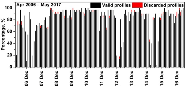
Figure 1 Monthly percentage of radiosonde data available during April 2006–May 2017 at Gadanki. The percentage of discarded profiles in each month is also shown in red.

2 Data and methodology

2.1 Data

In this study, long-term (11 years) observations of high-vertical-resolution radiosonde (Vaisälä RS-80, RS-92; Meisei RS-01GII, RS-6G, RS-11G, IMS-100) data are used to analyse CVS over a tropical station, Gadanki. There is no significant change in the accuracies of the meteorological parameters from these different radiosondes. Most of these radiosondes were launched around 17:30 local time (LT = UT + 05:30 h). In general, the balloons are not launched during moderate to heavy rain conditions. However, we have done a visual inspection of each radiosonde profile. The RH profiles which show continuous saturation with height were discarded. Figure 1 shows the monthly percentage of radiosonde data available from April 2006 to May 2017. In total, 3313 launches were made, out of which 98.9 % and 86.6 % reached altitudes greater than 12.5 and 20 km, respectively. The data which have a balloon-burst altitude less than 12.5 km (1.1 %) are discarded. Also, we have put a condition on the number of profiles in a month, which should be more than seven to represent that month. After applying these two conditions the total number of profiles was 3251. In addition, to study the diurnal variations in CVS over Gadanki, we made use of radiosonde observations taken from Tropical Tropopause Dynamics (TTD) campaigns (Venkat Ratnam et al., 2014b) conducted during the Climate and Weather of Sun Earth Systems (CAWSES) India Phase II programme (Pallamraju et al., 2014). During these campaigns, radiosondes were launched every 3 h for three continuous days in each month from December 2010 to March 2014 except in December 2012 and January, February, and April 2013.

2.2 Methodology

Several methods are employed to determine the CVS from the profiles of radiosonde data (Poore et al., 1995; Wang and Rossow, 1995; Chernykh and Eskridge, 1996; Minnis et al., 2005; Zhang et al., 2010). Poore et al. (1995) estimated the cloud base and cloud top using temperature-dependent dew-point depression thresholds. First, the dew-point depression must be calculated at every radiosonde level. According to Poore et al. (1995), a given atmospheric level has a cloud if ΔT_d<1.7 ^∘C at T>0 ^∘C, ΔT_d<3.4 ^∘C at 0>T>−20 ^∘C, and ΔT_d<5.2 ^∘C at T<−20 ^∘C.

Wang and Rossow (1995) used temperature, pressure, and RH profiles and computed RH with respect to ice instead of liquid water for the levels with temperatures lower than 0 ^∘C. To this new RH profile they have applied two RH thresholds (min RH = 84 % and max RH = 87 %). In addition, if RH at the base (top) of the moist layer is lower than 84 %, an RH jump exceeding 3 % must exist from the underlying (above) level. According to the Chernykh and Eskridge (1996) method, the necessary condition for the existence of clouds in a given atmospheric level is that the second derivatives with respect to height (z) of temperature and RH are positive and negative, respectively, i.e. $T^{\prime \prime }\left(z\right)\ge \mathrm{0}$ and ${\mathrm{RH}}^{\prime \prime }\left(z\right)\le \mathrm{0}$. Minnis et al. (2005) provided an empirical parameterization that calculates the probability of the occurrence of a cloud layer using RH and air temperature from radiosondes. First, RH values must be converted to RH with respect to ice when temperature is less than −20 ^∘C. Second, the profile has to be interpolated every 25 hPa up to the height of 100 hPa. An expression to estimate the cloud probability (Pcld) as a function of temperature and RH is then applied. In this expression, RH is given the maximum influence as it is the most important factor in cloud formation. Finally, a cloud layer is set wherever Pcld ≥ 67 %. The Zhang et al. (2010) method is an improvement on the Wang and Rossow (1995) method. Instead of a single RH threshold, Zhang et al. (2010) applied altitude-dependent thresholds without the requirement of the 3 % RH jump at the cloud base and top.

Costa-Suros et al. (2014) compared the CVS derived from these five methods described above by using 193 radiosonde profiles acquired at the Atmospheric Radiation Measurement (ARM) Southern Great Plains site during all seasons of the year 2009. The performance of the five methods has been assessed by comparing with Active Remote Sensing of Clouds (ARSCL) data taken as a reference. Costa-Suros et al. (2014) concluded that three of the methods (Poore et al., 1995; Wang and Rossow, 1995; Zhang et al., 2010) perform reasonably well, giving perfect agreement for 50 % of the cases and approximate agreements for 30 % of the cases. The other methods gave poor results (lower perfect and/or approximate agreement and higher false positive, false negative, or not coincident detections). Among the three methods, the Zhang et al. (2010) method is the most recent version of the treatment initially proposed in Poore et al. (1995) and Wang and Rossow (1995), and it provides good results (a perfect agreement of 53.9 % and an approximate agreement of 29.5 %). Thus, the algorithm of Zhang et al. (2010) is used for detecting cloud layers in our analysis.

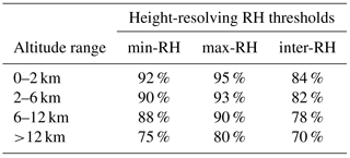
Cloud layers are associated with high RH values above some threshold as the radiosonde penetrates through them. The cloud detection algorithm of Zhang et al. (2010) employs three height-resolving RH thresholds to determine cloud layers: minimum and maximum RH thresholds in cloud layers (min-RH and max-RH) and minimum RH thresholds within the distance of two adjacent layers (inter-RH). The height-resolving thresholds of max-RH, min-RH, and inter-RH values are specified in Table 1. The algorithm begins by converting RH with respect to liquid water to RH with respect to ice at temperatures below 0 ^∘C (see example in Fig. 2). The accuracy of RH measurement is less than 5 % up to the altitude 12.5 km and hence the RH profile is examined from the surface to 12.5 km (∼200 hPa) of altitude to find cloud layers in seven steps: (1) the base of the lowest moist layer is determined as the level at which RH exceeds the min-RH corresponding to this level; (2) above the base of the moist layer, contiguous levels with RH over the corresponding min-RH are treated as the same layer; (3) the top of the moist layer is identified when RH decreases to below the corresponding min-RH or RH is over the corresponding min-RH but the top of the profile is reached; (4) moist layers with bases lower than 500 m a.g.l. (above ground level) and thickness less than 400 m are discarded; (5) the moist layer is classified as a cloud layer if the maximum RH within this layer is greater than the corresponding max-RH at the base of this moist layer; (6) two contiguous layers are considered as a one-layer cloud if the distance between these two layers is less than 300 m or the minimum RH within this distance is more than the maximum inter-RH value within this distance; and (7) clouds are discarded if their thicknesses are less than 100 m.

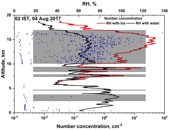
Figure 2 Results from a flight of RS-11G radiosonde and cloud particle sensor (CPS) sonde on the same balloon launched at 02:00 IST on 4 August 2017 at Gadanki, India. Profiles of RH estimated with respect to water (solid black line), ice (when temperatures are less than 0 ^∘C, solid red line), and number concentration (filled blue circles) from CPS sonde profile are shown. Detected cloud-layer boundaries are shown by the filled gray rectangular boxes. The increase in the number concentration within the detected cloud layers indicates that the cloud-layer boundaries detected in the present study are accurate.

Table 1 Summary of height-resolving RH thresholds.

At the measurement location, we have boundary-layer lidar (BLL) and Mie lidar. When there is an occurrence of multilayer configuration, BLL does not give an accurate cloud base altitude for higher layers. Mie lidar gives the vertical structure of cirrus clouds (usually occurring at higher altitude). Here, CVS is examined only up to 12.5 km of altitude as the accuracy of RH measurements is poor at higher altitudes. Also, Mie lidar is operated mostly during cloud-free conditions (only during cirrus cloud or clear sky conditions). Further, the timings of radiosonde and lidar measurements are different. Therefore, we did not compare with the ground-based lidar measurements. On the other hand, CloudSat–CALIPSO overpasses of the experiment location are around 02:00 and 14:00 LT, whereas regular radiosonde launches are around 17:30 LT. Therefore, we did not compare the CVS derived from regular radiosonde and CloudSat–CALIPSO measurements. However, we have 3-hourly radiosonde observations for three continuous days in every month during TTD campaigns. We did not get collocated (space and time) measurements from CloudSat–CALIPSO and radiosonde during these campaigns.

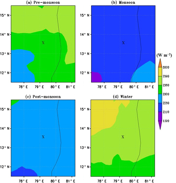
Figure 3 Seasonal mean distribution of OLR around the Gadanki location observed during (a) pre-monsoon, (b) monsoon, (c) post-monsoon, and (d) winter seasons averaged during 2006–2017. The symbol “X” indicates the location of Gadanki.

Before proceeding further, it is desired to verify whether the identified layers of clouds are correct or not with independent observations. For that we have launched cloud particle sensor (CPS) sonde (Fujiwara et al., 2016) at Gadanki, which provides a profile of cloud number concentration. Results from a flight of RS-11G radiosonde and cloud particle sensor (CPS) sonde on the same balloon launched at 02:00 LT on 4 August 2017 at Gadanki, India, are shown in Fig. 2. A sudden increase in the cloud number concentration within the detected cloud layers indicates that the cloud-layer boundaries detected in the present study are in good agreement.

The drawback of using the radiosonde data for detecting the CVS at a given location is the radiosonde horizontal displacement due to the drift produced by the wind. However, irrespective of the season, the maximum horizontal drift of radiosonde when it reaches the 12.5 km of altitude is always less than 20 km (Venkat Ratnam et al., 2014a). One may expect different background features within this 20 km, particularly localized convection, that may influence the CVS. In order to assess this aspect, we used outgoing longwave radiation (OLR) as a proxy for tropical convection. Figure 3a–d show the seasonal mean distribution of OLR (from KALPANA-1 satellite) around the Gadanki location obtained during the pre-monsoon, monsoon, post-monsoon, and winter seasons averaged during 2006–2017. It can be noted that irrespective of the season, homogeneous cloudiness prevailed for more than a 50 km radius around the Gadanki location. Hence, the CVS detected from the radiosonde can be treated as representative of the Gadanki location.

The methodology described in Sect. 2.2 to detect CVS is applied on high-vertical-resolution radiosonde data acquired during April 2006 to May 2017 from Gadanki, as well as special radiosondes launches during TTD campaigns from December 2010 to March 2014. Results are presented in Sect. 4. Before going further, it is desirable to examine the background meteorological conditions prevailing over Gadanki during different seasons.

3 Background meteorological conditions

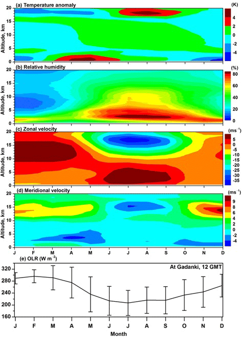
Figure 4 Time–altitude cross sections of monthly mean (a) temperature anomaly, (b) relative humidity, (c) zonal wind, and (d) meridional wind observed over Gadanki using radiosonde observations during April 2006 to May 2017. (e) Monthly mean outgoing longwave radiation (OLR) over Gadanki obtained using KALPANA-1 data during April 2006 to May 2017 along with standard deviation (vertical bars).

The National Atmospheric Research Laboratory (NARL) at Gadanki is located about 120 km north-west of Chennai (Madras) on the east coast of the southern Indian peninsula. This station is surrounded by hills with a maximum altitude of 350–400 m above the station, and the station is at an altitude of 375 m a.m.s.l. (hereinafter all altitudes are mentioned above mean sea level). The local topography is complex with a number of small hillocks around and a high hill of ∼1 km about 30 km from the balloon launching site in the north-east direction. The detailed topography of Gadanki is shown in Basha and Ratnam (2009). Gadanki receives about 53 % of the annual rainfall during the south-west monsoon (June to September) and 33 % of the annual rainfall during the north-east monsoon (October to December) (Rao et al., 2008a). The rainfall during the south-west monsoon occurs predominantly from the evening to midnight period. About 66 % of total rainfall is convective in nature, while the remaining rain is widespread stratiform in character (Rao et al., 2008a).

Background meteorological conditions prevailing over the observational site are briefly described based on the radiosonde data collected during April 2006 to May 2017. The seasons are classified as winter (December–January–February), pre-monsoon (March–April–May), monsoon (June–July–August–September), and post-monsoon (October–November). The climatological monthly mean contours of the temperature anomalies, relative humidity, and zonal and meridional winds are shown in Fig. 4a–d, respectively. From the surface to 1 km of altitude, temperature anomalies show seasonal variability with warmer temperatures during pre-monsoon months and relatively lower temperatures during the winter season (Fig. 4a). Temperature anomalies do not show significant seasonal variation from 1 km of altitude to the middle troposphere, but significant seasonal differences are observed in the lower stratosphere. There are significant seasonal variations in the RH (Fig. 4b). During winter, RH is small (40–50 %) from the surface to ∼3 km of altitude and is almost negligible above. However, during the other seasons, particularly in the peak monsoon months (July and August), large RH values (60–70 %) are noticed up to 10 km of altitude.

During winter, easterlies are observed up to 4–6 km of altitude and westerlies above (Fig. 4c). There seem to be weak easterlies between 14 and 20 km of altitude during the pre-monsoon. During the monsoon season low-level westerlies exist below 7–8 km and easterlies above. The Tropical Easterly Jet (TEJ) is prevalent over this region in the SW monsoon season, with peak velocity sometimes reaching more than 40 m s⁻¹ (Roja Raman et al., 2009). There are large vertical shears during the monsoon in the zonal wind. Easterlies exist up to 20 km of altitude during the post-monsoon season. In general, meridional velocities are very small and northerlies are observed up to 8 km and southerlies above in all the seasons, except during the monsoon (Fig. 4d). During the winter and monsoon, relatively stronger southerlies and northerlies prevailed, respectively, between 12 and 15 km of altitude. A clear annual oscillation can be noticed in both zonal and meridional velocities. Similar variations are also observed by the MST radar located at the same site between 4 and 20 km (Venkat Ratnam et al., 2008; Basha and Ratnam, 2013; Nath et al., 2009). Monthly mean OLR around Gadanki at 17:30 LT is shown in Fig. 4e. Low values of OLR (<220 W m⁻²) around the Gadanki location indicate that the occurrence of very deep convection during the monsoon season, consistent with the occurrence of high RH values up to 10 km of altitude during the monsoon season (Fig. 4b).

4 Results

By adopting the methodology described in Sect. 2.2 we have detected a total of 4309 cloud layers from 3251 radiosonde launches at the Gadanki location during the period of data analysis. For each season, cloud layers during April 2006–May 2017 are averaged to obtain the composite picture of CVS. Seasonal variability in cloud layers is discussed in Sect. 4.2.

4.1 Diurnal variation of single-layer and multilayer clouds

There are studies on the diurnal variation of cloud layers outside the Indian region, for example over Porto Santo Island during the Atlantic Stratocumulus Transition Experiment (ASTEX) by Wang et al. (1999), over San Nicolas Island during the First ISCCP Regional Experiment (FIRE) by Blaskovic et al. (1990), and over Shouxian (32.56^∘ N, 116.78^∘ E) by Zhang et al. (2010). To the authors' knowledge there are no studies on the diurnal variability of cloud layers over the Indian region. For the first time over the Indian region, the diurnal variability of cloud layers is studied by using radiosonde observations taken from TTD campaigns. Figure 5a–d describe the diurnal variations of single-layer and multilayer clouds during the pre-monsoon, monsoon, post-monsoon, and winter seasons over the Gadanki region. As mentioned in Sect. 2.1, from December 2010 to March 2014, we have launched radiosondes every 3 h for three continuous days in every month except during December 2012 and January, February, April, 2013. The total number of profiles taken during the pre-monsoon, monsoon, post-monsoon, and winter seasons are 160, 254, 101, and 199, respectively. Among these the number of cloudy profiles are 93 in the pre-monsoon, 241 in the monsoon, 63 in the post-monsoon, and 96 in the winter season.

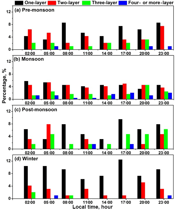
Figure 5 Diurnal variations of one-layer, two-layer, three-layer, and four- or more-layer clouds observed during (a) pre-monsoon, (b) monsoon, (c) post-monsoon, and (d) winter seasons.

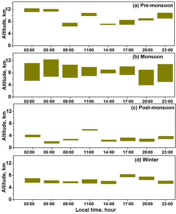
Figure 6 Diurnal variations of mean vertical locations (base and top) and thicknesses of one-layer clouds observed during (a) pre-monsoon, (b) monsoon, (c) post-monsoon, and (d) winter seasons.

Figure 7 Diurnal variations of mean vertical locations (base and top) and thicknesses of two-layer clouds observed during (a) pre-monsoon, (b) monsoon, (c) post-monsoon, and (d) winter seasons.

From Fig. 5a–d for four seasons, diurnal variations of cloud occurrence show a maximum between 23:00 and 05:00 LT and a minimum at 14:00 LT, except during the monsoon season. During the monsoon season, a minimum in cloud occurrence occurred at 11:00 LT. Using infrared brightness temperature data over the Indian region Gambheer and Bhat (2001), Zuidema (2003), and Reddy and Rao (2018) observed the maximum frequency of occurrence of clouds during late night to early morning hours. The percentage of occurrence of one-layer and multilayer clouds shows noticeable diurnal variations in all seasons except in the monsoon season. The maximum percentage of occurrence in one-layer clouds is at 08:00 LT in the pre-monsoon season and it is at 17:00 LT during the post-monsoon and winter seasons. For all the seasons, the maximum percentage of occurrence in multilayer clouds is between 20:00 and 05:00 LT. Figure 6a–d describe the mean vertical locations (base and top) and cloud thicknesses of one-layer clouds during the pre-monsoon, monsoon, post-monsoon, and winter seasons, respectively. During the monsoon season, the maximum in cloud top altitude is at 05:00 LT and the minimum is at 14:00 LT (Fig. 6b). In general, the cloud base of one-layer cloud occurs at higher altitude between 11:00 and 14:00 LT and it occurs at relatively low altitudes between 20:00 and 08:00 LT. Except during the post-monsoon season, single-layer clouds are high-level clouds with a base at greater than 5 km most of the time. During the post-monsoon season, single-layer clouds are low-level at 05:00 LT (cloud base altitude of 1.4 km) and middle-level clouds between 14:00 and 02:00 LT (Fig. 6c). During the pre-monsoon and monsoon seasons, the thickness of single-layer clouds reaches a maximum at 23:00 LT and a minimum at 14:00 LT (Fig. 6a, b). The minimum in one-layer cloud thickness at 14:00 LT is due to the increase in cloud base altitude and simultaneous decrease in cloud top altitude. There is not much variability in the thickness of one-layer clouds during the post-monsoon and winter seasons (Fig. 6c, d). Figure 7a–d and Fig. S1a–d in the Supplement are the same as Fig. 6a–d but for two-layer and three-layer clouds. Similar to one-layer cloud, the cloud base of the bottom layer of two-layer clouds shows a maximum between 11:00 and 14:00 LT and a minimum between 20:00 and 08:00 LT. The thickness of the top layer and bottom layer of two-layer clouds reaches a minimum value between 11:00 and 14:00 LT. The upper layer of two-layer clouds shows a maximum in thickness at 23:00 LT and minimum at 11:00 LT during the monsoon season (Fig. 7b).

Cloud maintenance and development are strongly modulated by diabatic processes, namely solar heating and longwave (LW) radiative cooling (Zhang et al., 2010). Near noontime (11:00–14:00 LT), solar heating is so strong that (1) evaporation of cloud drops may occur and (2) atmospheric stability may increase, thus suppressing cloud development. So near noontime, the vertical development of single-layer clouds and the vertical development of the uppermost layer of multiple layers of cloud are suppressed due to solar heating. This effect is predominant during the monsoon season for one-layer and two-layer clouds (Figs. 6b and 7b) and during the pre-monsoon and post-monsoon seasons for three-layer clouds (Fig. S1a, c). However, for lower layers of cloud in a multiple-layer cloud configuration, solar heating is greatly reduced because of the absorption and scattering processes of the upper layers of cloud. In general the maximum in surface temperature occurs around 15:20 LT (Reddy and Rao, 2018). The ground surface is warmer than any cloud layer so through the exchange of LW radiation, the cloud base gains more energy. This facilitates cloud development and leads to a maximum in cloud altitude and thickness between 14:00 and 17:00 LT (Figs. 7a, b, d, and S1a). This effect is predominant during the winter season for two-layer clouds (Fig. 7d) and during the pre-monsoon season for three-layer clouds (Fig. S1a). As the sun sets, LW radiative cooling starts to dominate over shortwave (SW) radiative warming. Cloud top temperatures begin to lower, which increases atmospheric instability and fuels the development of single-layer clouds and the uppermost layer of cloud in multiple-layer cloud configurations. At sunset, solar heating diminishes and LW cooling strengthens, which may explain why there is a peak between 20:00 and 23:00 LT in the thickness of one-layer clouds and the uppermost layer of two-layer cloud. This effect is clearly observed in the monsoon season (Figs. 6b, 7b, S1b). We conclude that diurnal variability in the base, top, and thickness for single-layer, two-layer, and three-layer clouds is significant. Hence there can be a bias in cloud vertical structure when we are studying the composite over a season by using polar satellites.

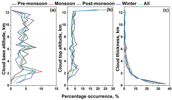
Figure 8 Percentage of occurrence of the (a) cloud base altitude, (b) cloud top altitude, and (c) cloud thickness observed during different seasons over Gadanki. Altitude bin size is 500 m.

In the next section, we show the seasonal variability in cloud layers using long-term (11 years) observations of high-vertical-resolution radiosonde over Gadanki. Note that most of these radiosondes were launched around 17:30 LT and hence there will be bias in the results due to the diurnal variability of cloud layers, which we have discussed above. Hence the results related to the seasonal variability of cloud layers are only representative of 17:30 LT.

4.2 Seasonal variability in the cloud layers

Figure 8a–c describe the percentage of occurrence of the base, top, and thickness of cloud layers observed during different seasons over Gadanki. The cloud base altitude shows a bimodal distribution in all seasons except during the pre-monsoon season (Fig. 8a). During the pre-monsoon season, the peak of cloud base altitude distribution is observed at ∼6.2 km (∼7.5 %). During the other three seasons (monsoon, post-monsoon, and winter), the first peak in cloud base altitude is observed between 2 and 3 km of altitude and the second peak is observed at ∼6.2 km. Using CloudSat observations over the Indian monsoon region, Das et al. (2017) also reported that the cloud base altitude over the Indian monsoon region shows a bimodal distribution. However, the first peak in cloud base altitude is observed at ∼14 km, while the second maximum is at 2 km.

The cloud top altitude increases above 12 km of altitude and has a maximum at 12.5 km in all seasons (Fig. 8b). Note that we restrict maximum altitude to 12.5 km due to limitation in providing reliable water vapour above that altitude from normal radiosondes. At lower altitudes, during the monsoon season the peak in cloud top altitude is at 2.9 km and it increases to 3.3 km during the post-monsoon season. However, we have also checked the cloud vertical structure until 18 km. There is no significant difference in the cloud base and cloud top altitude distribution (See Fig. S2). Das et al. (2017) reported that there are two peaks in the cloud top altitude: one at ∼17 km and other at ∼3 km. The peaks in cloud base and cloud top at higher altitudes as observed by Das et al. (2017) could be due to the occurrence of cirrus clouds.

Figure 9 Mean vertical locations (base and top), cloud thicknesses, and percentage of occurrence of (a) low-level clouds, (b) middle-level clouds, (c) high-level clouds, and (d) deep convective clouds observed during different seasons.

The cloud base altitude values are subtracted from the cloud top altitude for each cloud layer to extract the cloud thickness. Figure 8c describes the percentage of occurrence of cloud thickness observed during different seasons. The occurrence of thicker clouds decreases exponentially. The cloud thickness has a maximum below 500 m for all seasons, which constituted about 34.7 %, 26.5 %, 31.2 %, and 36.6 % of the total observed cloud layers during the pre-monsoon, monsoon, post-monsoon, and winter seasons, respectively. In general, for all seasons, more than 65 % of cloud layers have cloud thickness <2 km.

Different cloud types occurring at different height regions have a spectrum of effects on the radiation budget (Behrangi et al., 2012). Therefore, the clouds have been classified into four groups based on the cloud base altitude and their thickness (Lazarus et al., 2000; Zhang et al., 2010): (1) low-level clouds with bases lower than 2 km and thickness less than 6 km; (2) middle-level clouds with bases ranging from 2 to 5 km; (3) high-level clouds with bases greater than 5 km; and (4) deep convective cloud (hereafter called DCC) with a base less than 2 km and thicknesses greater than 6 km. These four types of clouds account for 11.97 %, 26.71 %, 59.36 %, and 1.95 % of all cloudy cases, respectively. Figure 9a–d describe the mean vertical locations (base and top), cloud thicknesses, and percentage of occurrence of low-, middle-, and high-level clouds and DCC observed during different seasons. At the Gadanki location, there is a distinct persistence of high-level clouds over all the seasons. The occurrence of high-level clouds is 69.05 %, 58.49 %, 55.5 %, and 58.6 % during the pre-monsoon, monsoon, post-monsoon, and winter seasons, respectively (Fig. 9c). In general, after the dissipation of deep convective clouds they spread large anvils and persist as high-level clouds for a longer duration. These high-level clouds could be due to in situ generated convective systems or propagated from the surrounding oceans. Zuidema (2003) reported that the deep convective systems generated over the central and western Bay of Bengal (BoB) advect toward the inland region of southern peninsular India and dissipate. In general, the high-level clouds follow background winds at those levels. Especially during the monsoon season due to the strong westerly winds in the upper levels, high-level clouds which originate from MCS over BoB advect into the Indian region and contribute to the high-level cloud occurrence. Hence the outflow caused by deep convective systems could be responsible for the higher percentage of occurrence of high-level clouds. Low-level (middle-level) clouds contribute about 3.74 %, 10.45 %, 16.27 %, and 20.89 % (27.04 %, 29.35 %, 24.28 %, and 18.67 %) of all cloudy cases during the pre-monsoon, monsoon, post-monsoon, and winter seasons, respectively (Fig. 9a, b).

The thicknesses of low-, middle-, and high-level clouds have minimum values during the winter season and maximum values in the monsoon season (Fig. 9a–c). DCCs have a minimum thickness in winter and a maximum in the pre-monsoon season (Fig. 9d). The average cloud base (cloud top) altitudes for low-, middle-, and high-level clouds and deep convective clouds are 1.74 km (3.16 km), 3.59 km (5.55 km), 8.79 km (10.49 km), and 1.22 km (11.45 km), respectively. Over the Indian summer monsoon region, Das et al. (2017) reported that the percentage of occurrence of high-level clouds is more than the other three cloud types. Over Shouxian (32.56^∘ N, 116.78^∘ E), Zhang et al. (2010) reported that the percentage of occurrence of low-, middle-, and high-level clouds and deep convective clouds is 20.1 %, 19.3 %, 59.5 %, and 1.1 %, respectively.

Figure 10 Percentage of occurrence of (a) one-layer, (b) two-layer, (c) three-layer, and (d) four- or more-layer clouds observed during different seasons.

4.2.1 Single-layer and multilayer clouds

By interacting with both shortwave and longwave radiation, clouds play a crucial role in the radiative budget at the surface, within, and at the top of the atmosphere. Over the tropics, the zonal mean net cloud radiative effect differences between multilayer clouds and single-layer clouds were positive and dominated by shortwave cloud radiative effect differences (Li et al., 2011). This is because multilayer clouds reflect less sunlight to the top of the atmosphere and transmit more to the surface and within the atmosphere than single-layer clouds as a whole. As a result, multilayer clouds warm the Earth–atmosphere system when compared to single-layer clouds (Li et al., 2011). In this study, we studied the occurrence of single-layer and multilayer clouds obtained during different seasons at the Gadanki location. The percentage of occurrence of single-layer, two-layer, three-layer, and four- or more-layer clouds during the pre-monsoon, monsoon, post-monsoon, and winter seasons is shown in Fig. 10a–d. Single-layer, two-layer, and three-layer clouds account for 40.80 %, 30.71 %, and 19.68 % of all cloud configurations, respectively. Despite the low frequency of occurrence of one-layer clouds over Gadanki, they exhibit pronounced seasonal variation in magnitude with very low frequency during the pre-monsoon season. This may be due to the strong warm and dry atmospheric conditions from the surface to the boundary-layer top (Fig. 4a, b). The percentage of occurrence of single-layer (multilayer) clouds during the pre-monsoon, monsoon, post-monsoon, and winter seasons is 7.7 %, 14.2 %, 8.48 %, and 10.42 % (7.93 %, 34.58 %, 10.83 %, and 5.86 %), respectively. There is a significant occurrence of multilayer clouds during the monsoon season compared to the other seasons, indicating that the development of multilayer clouds is favourable under warm and moist atmospheric conditions (Fig. 4a, b). Among the different cloud layers, two-layer clouds have a maximum percentage of occurrence (16.6 %) during the monsoon season (Fig. 10b). Luo et al. (2009) reported the occurrence of multilayer clouds over the Indian region during the summer season and attributed it to the complex cloud structure associated with the monsoon system. Zhang et al. (2010) reported that multilayer cloud occurrence frequency is relatively higher during summer months (June, July, and August) than autumn months (September, October, and November) over Shouxian. Recently, Using the 4 years of combined observations of CloudSat and CALIPSO, Subrahmanyam and Kumar (2017) reported the maximum frequency of occurrence of two-layer clouds over the Indian subcontinent during June, July, and August. This they attributed to the presence of Indian summer monsoon circulation over this region, which is dominated by the formation of various kinds of clouds such as cumulus, stratocumulus, and cirrus. Very recently, George et al. (2018) reported CVS using radiosonde launches during depression and non-depression events in the south-west monsoon season using 1 month of field campaign data over Kanpur, India.

Table 2 Mean base, top, and thicknesses of cloud layers of single-layer, two-layer, and three-layer clouds.

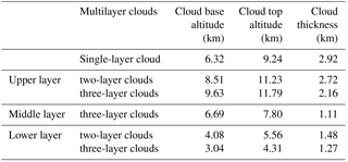
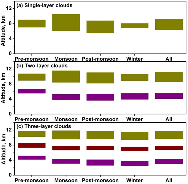
Figure 11 Mean vertical locations (base and top) and cloud thicknesses of (a) one-layer clouds, (b) two-layer clouds, and (c) three-layer clouds observed during different seasons.

Figure 11a–c describe the mean vertical locations (base and top) and cloud thicknesses of single-layer, two-layer, and three-layer clouds during different seasons. Except during the winter season, single-layer clouds are thicker than the layers forming multilayer clouds. Also, upper-layer clouds are thicker than lower-layer clouds in multilayer clouds. This could be due to the exchange of longwave radiation between the cloud base of the upper layer and the cloud top of the lower layer. As a result, there is a strong reduction in longwave radiation cooling at the top of the lower layer of cloud in the presence of upper layers of cloud (Zhang et al., 2010; Wang et al., 1999; Chen and Cotton, 1987).

Irrespective of the season, single-layer clouds are high-level clouds; i.e. the cloud base is >5 km (Fig. 11a). Maximum cloud top altitude and cloud thickness occurred during the monsoon season for single-layer clouds (Fig. 11a) and the uppermost layer of multilayer cloud configurations (Fig. 11b, c). This is consistent with the low OLR values (<220 W m⁻²) observed during the monsoon season (Fig. 4e). Except during the pre-monsoon season, the cloud base, cloud top, and cloud thickness values of the lower layer of multilayer clouds are the same during the monsoon, post-monsoon, and winter seasons. During the pre-monsoon season, the cloud base and cloud top of the lower layer of multilayer clouds occurred at relatively higher altitudes (Fig. 11b, c). Similarly, there are no significant variations in cloud thickness in the middle layer of three-layer clouds between the seasons. However, the cloud base and cloud top of the middle layer of three-layer clouds during the pre-monsoon season occurred at relatively higher altitudes than the other three seasons (Fig. 11c). Table 2 describes the mean base, top, and thicknesses of cloud layers of single-layer, two-layer, and three-layer clouds. In two-layer clouds, the thickness of the upper-level cloud layer is about the same as that of single-layer clouds. In three-layer clouds, the base and top heights of the lowest layer of cloud are similar to those of the lowest layer of cloud in two-layer clouds.

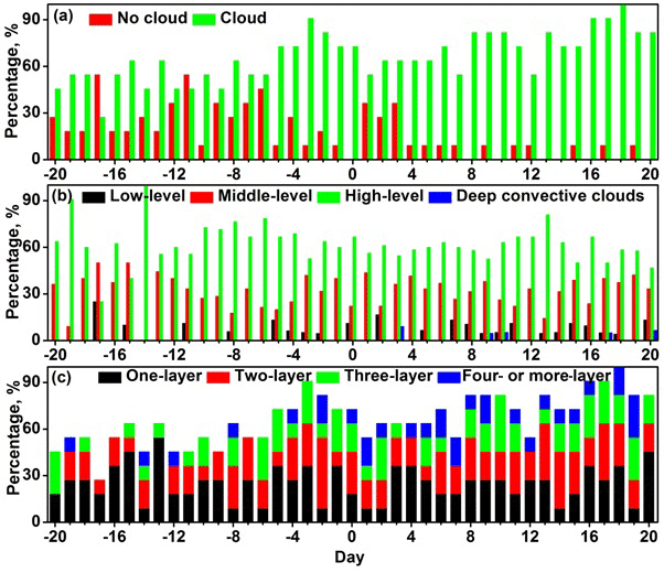
Figure 12 Composite (2006–2016) percentage of occurrence of (a) clear and cloud conditions, (b) low-level, middle-level, high-level, and deep convective cloud, and (c) one-, two-, three-, and four- or more-layer clouds observed with respect to the date of monsoon arrival over the Gadanki location. Zero on the x axis indicates the date of monsoon arrival over the Gadanki location.

4.3 Variability in CVS with respect to SW monsoon arrival over Gadanki

CVS plays an important role in the summer monsoon because it can significantly affect the atmospheric heat balance through latent heating caused by water phase changes and through the scattering of radiation. In this section we discuss the variability in different clouds with respect to the date of arrival of the south-west (SW) monsoon over Gadanki. SW monsoon onset occurs over the Kerala coast (south-west coast of India) during the last week of May or first week of June. In general, the climatological mean monsoon onset over Kerala (MOK) is on 1 June with ±7 days. It is to be noted that the climatological onset date is obtained from IMD long-term onset dates and the arrival date over Gadanki is picked up manually from the yearly onset date lines over the India map given by IMD.

Figure 12 shows the composite (2006–2016) percentage of occurrence of clear sky and cloud days (Fig. 12a), low-level, middle-level, high-level, and deep convective clouds (Fig. 12b), and one-, two-, three-, and four- or more-layer clouds (Fig. 12c) with respect to monsoon arrival date. Figure 13a and b describe the mean vertical locations (base and top) and cloud thicknesses of single-layer and two-layer clouds with respect to monsoon arrival date. Day zero in Figs. 12a, b and 13a, b indicates the date of monsoon arrival over the Gadanki location. The percentage of occurrence of clear sky conditions prior to the monsoon arrival over the Gadanki location decreases and reduces to zero on the date of monsoon arrival (Fig. 12a). This indicates that the estimated dates of monsoon arrival over the Gadanki location are correct. From day 4 onwards the cloudiness start increases and peaks on day 18 (Fig. 12a). The percentage of occurrence of middle-level clouds decreases until 5 days prior to the monsoon arrival (Fig. 12b). Subsequently, the middle-level cloud percentage increases and does not show significant variability after the monsoon arrival. There are no deep convective clouds prior to and during the monsoon arrival over the Gadanki location (Fig. 12b). They occurred on days 3, 9, 10, 17, and 20. During and after the arrival of the monsoon, the percentage of occurrence of multilayer clouds is always greater than the single-layer clouds except on days 3 and 4 (Fig. 12c). On day zero it is noted that single-layer clouds are high-level clouds and they are thicker with thickness ∼6.7 km (Fig. 13a). In two-layer clouds the bottom layer is middle-layer cloud and the top layer is high-level cloud (Fig. 13b). The bottom layer is thicker than the top layer. During deep convective clouds and middle-level clouds, single-layer clouds prevailed. The thickness of single-layer clouds shows large variability with thickness ranging from 300 m to 5 km during the first week after the arrival of the monsoon. In the second week, the thickness ranges from 2 to 5 km (Fig. 13a). After the arrival of the monsoon, the thickness of the bottom layer in two-layer cloud is relatively higher than the top layer (Fig. 13b). Thicker single-layer clouds and the bottom layer of two-layer clouds after the monsoon arrival over Gadanki is due to the increase in tropospheric water vapour.

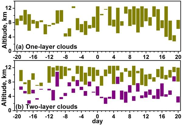
Figure 13 Composite (2006–2016) variations of mean vertical locations (base and top) and thicknesses of one-layer clouds and two-layer clouds observed with respect to the date of monsoon arrival over the Gadanki location. Zero on the x axis indicates the date of monsoon arrival over the Gadanki location.

5 Summary

Cloud vertical structure (CVS) is studied for the first time over India using long-term high-vertical-resolution radiosonde measurements at the Gadanki location obtained during April 2006 to May 2017. In order to obtain diurnal variation in CVS, we have used 3-hourly launched radiosondes for 3 days in each month during December 2010 to March 2014. CVS is obtained following Zhang et al. (2010) whereby it relies on height-resolved relative humidity thresholds. After obtaining the cloud layers they are segregated into low-, middle-, and high-level clouds depending upon their altitude of occurrence. Detected layers are verified using independent measurements from cloud particle sensor (CPS) sonde launched from the same location. A very good match between these two independent measurements is noticed.

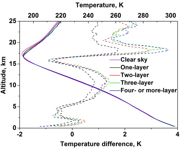
Figure 14 Composite (2006–2016) temperature profiles during clear sky, one-layer, two-layer, three-layer, and four- or more-layer cloud occurrences. The respective temperature difference profiles from clear sky conditions are shown with dashed lines.

First, the diurnal variations in CVS over Gadanki are studied using radiosonde observations taken from TTD campaigns conducted during the CAWSES India Phase II programme. During the pre-monsoon and monsoon seasons, the thickness of single-layer clouds reaches a maximum at 23:00 LT and a minimum at 14:00 LT. The upper layer of two-layer clouds shows a maximum in thickness at 23:00 LT and a minimum at 11:00 LT during the monsoon season. Radiosonde measurements around 17:30 LT were used to study the seasonal variability in CVS. After ascertaining the cloud layers they are segregated into different seasons to obtain the seasonal variation of CVS. High-level clouds account for 69.05 %, 58.49 %, 55.5 %, and 58.6 % of cloud layers identified during the pre-monsoon, monsoon, post-monsoon, and winter seasons, respectively, indicating that high cloud layers are most prevalent at the Gadanki location. Single-layer, two-layer, and three-layer clouds account for 40.80 %, 30.71 %, and 19.68 % of all cloud configurations, respectively. Multilayer clouds occurred more frequently during the monsoon with 34.58 %. Maximum cloud top altitude and cloud thickness occurred during the monsoon season for single-layer clouds and the uppermost layer of multilayer cloud configurations.

Further, we have discussed the variability in different clouds with respect to the date of arrival of the south-west (SW) monsoon over the Gadanki location. Prior to, during, and after the SW monsoon arrival over the Gadanki location, high-level cloud occurrence is more than the other cloud types. The middle-level cloud occurrence decreases until 5 days prior to the monsoon arrival and subsequently increases. There are no deep convective clouds prior to and during the monsoon arrival over the Gadanki location. The thickness of single-layer clouds shows large variability during the first week after the arrival of the monsoon. But it increases significantly between 8 and 11 days after the monsoon arrival. After the arrival of the monsoon, the thickness of the bottom layer in two-layer cloud is relatively higher than the top layer. Thicker single-layer clouds and the bottom layer of two-layer clouds after the monsoon arrival over Gadanki is due to the increase in tropospheric water vapour.

These cloud layers are expected to significantly affect the background temperature in the troposphere and lower stratosphere. The composite (2006–2016) temperature profiles during clear sky, one-layer, two-layer, three-layer, and four- or more-layer cloud occurrences are shown in Fig. 14. The temperature differences between the cloudy (single, two, three, four or more layers) and clear sky conditions are shown with dashed lines in Fig. 14. The striking result here is the occurrence of peak cooling (peak warming) below (above) the cold-point tropopause (CPT) altitude. The magnitude of cooling (warming) increases from single-layer to four- or more-layer cloud occurrence. The peak cooling and warming during four- or more-layer cloud occurrence are 0.9 K (at 15.7 km) and 3.6 K (at 18.1 km). Both single-layer and multilayer clouds show warming between 5 and 14.5 km of altitude. Peak warming of 0.8 K at 9.5 km for single-layer cloud and 1.3 K at 10.2 km for multilayer clouds is observed and these altitudes are close to the cloud top altitude of single-layer cloud and the top layer of multilayer clouds (Table 2). A detailed study on the impact of single-layer and multilayer clouds on UTLS dynamics and thermodynamics will be the subject of our subsequent article, including their radiative forcing.