Alkaline dust deposition to foliage surfaces likely enhances the dry deposition velocity of SO₂: an investigation in the Alberta Oil-Sands Region using the GEM-MACH air-quality model

We examine the potential impact of alkaline particle deposition on foliage and its influence on sulphur dioxide dry deposition velocities, using a new theoretical development, a high resolution air-quality model, and comparisons to observations. Our study domain encompasses the Athabasca Oil Sands Region, an industrial area where base cation-bearing fugitive dust from open-pit mining and forest fires coexists with elevated SO₂ emissions from large stacks. Our pH-modulated dry deposition scheme links thin aqueous films on foliage to local chemical conditions, including alkaline dust accumulation. We present the mechanism's theoretical basis, along with a simplified algorithm predicting foliage water pH and linked to SO₂ deposition velocities.

We predict enhanced SO₂ deposition, due to increased leaf surface pH from dust co-deposition near major dust sources, often by more than 1 cm s⁻¹. These result in dry deposition fluxes 2.5 to 10 times greater than in the absence of these effects – consistent with estimates from aircraft studies. The enhanced deposition reduces surface SO₂ concentrations by up to 60 % near sources, improves agreement with continuous monitoring data, and reduces the normalized mean bias at several stations. Taylor diagram statistics show improved model temporal variability performance. Further from sources of base-cation-containing dust, aqueous films on foliage remain acidic, reducing SO₂ deposition velocity and increasing concentrations.

We make specific recommendations for new observation data which would reduce formulation uncertainties. The findings have broad implications for global SO₂ budgets, given the significant role of wind-blown mineral dust and forest fire base cation emissions in influencing atmospheric acidity and trace gas removal.

1 Introduction

1.1 Phase 4 of the Air Quality Model Evaluation International Initiative

Recent intercomparisons between regional air-quality model predictions and observations in both North America and Europe under the AQMEII4 initiative (Makar et al., 2025) have shown that these regional models have a tendency towards positive biases in the concentrations of sulphur dioxide (SO₂) and particulate sulphate. One possible cause of these positive biases are underestimates in the deposition velocity of SO₂, which if corrected would result in lower SO₂ concentrations and hence reduced production of particulate sulphate via SO₂ oxidation. Enhanced deposition of SO₂ through its co-deposition with ammonia (NH₃) has been reported in the past (cf. Fowler et al., 2001; Flechard et al., 1999; Nemitz et al., 2001). However, in addition to ammonia, substantial deposition fluxes of other reactive base cations in the form of depositing dust have been recorded (Scheuvens et al., 2013; Wang et al., 2005; Avila et al., 1998; Rosas et al., 2025). These deposition fluxes may also influence the rate of SO₂ deposition. However, a detailed process description of this influence has been heretofore unavailable. We examine here the potential for simultaneous co-deposition of multiple base cations and acidic gases including SO₂, making use of a case study domain in the Athabasca Oil Sands Region, reporting the results as part of the AQMEII4 special issue on deposition.

1.2 Deposition in the Athabasca Oil Sands Region – Evidence for pH-modulation

The Athabasca Oil Sands Region (AOSR) in northeastern Alberta, Canada contains one of the world's largest bitumen reserves, spanning approximately 142 000 km² (Government of Alberta, 2025). It is well established that this region is a significant source of various gaseous and particulate emissions (You et al., 2024; Zhang et al., 2018a; Li et al., 2017). Among these, sulphur dioxide (SO₂) has drawn particular attention due to its known potential to adversely impact ecosystem health. SO₂ plays a central role in the development of acid rain (Irwin and Williams, 1988; Clarke and Radojevic, 1987) and acid fog (Pandis and Seinfeld, 1989; Munger et al., 1983), both of which have been implicated in widespread ecosystem degradation throughout the world (Hames et al., 2002; Cape, 1993; Cox et al., 1989; Schindler et al., 1989; Gilbert, 1986; Hutchinson and Whitby, 1977). An input of excess SO₂ and particle sulphate (SO${}_{\mathrm{4}}^{\mathrm{2}-}$) onto plant foliage can disrupt metabolic function (Rennenberg, 1984; Knabe, 1976), cause irreversible damage to guard cells that regulate stomatal activity (Knabe, 1976), and may lead to leaf necrosis or plant mortality in sensitive species (Hutchinson and Whitby, 1977; Gordon and Gorham, 1963).

Two recent measurement campaigns in the AOSR investigated dry deposition of oxidized sulphur. The first was an aircraft-based study (13 August to 7 September 2013; Hayden et al., 2021), which showed that dry deposition fluxes of total oxidized sulphur (SO₂ + particulate SO₄) decrease exponentially with increasing distance downwind from major AOSR sources. Their inferred deposition fluxes were 2 to 14 times higher than predicted by the GEM-MACH model (Makar et al., 2018), with inferred SO₂ deposition velocities ($V_{{\mathrm{a}}_{{\mathrm{SO}}_{\mathrm{2}}}}$) of 1.2 to 3.4 cm s⁻¹, compared to modelled values of 0.58 to 0.72 cm s⁻¹. Additional ground-based measurements at Fort McKay (6 to 8 June 2018) yielded even higher median $V_{{\mathrm{d}}_{{\mathrm{SO}}_{\mathrm{2}}}}$ values (median: 4.1 cm s⁻¹; range: 2.9 to 5.3 cm s⁻¹). Both the aircraft and Fort McKay tower data reflect daytime conditions. The second study (Gordon et al., 2023) involved continuous tower based SO₂ measurements from July to October 2021 at a forest site approximately 40 km north of Fort McMurray (located within the AOSR). Using the flux-gradient method, they reported inferred $V_{{\mathrm{d}}_{{\mathrm{SO}}_{\mathrm{2}}}}$ values of 2.1 to 5.9 cm s⁻¹ (mean: 4.6 cm s⁻¹), in agreement with the range reported by Hayden et al. (2021). These data may include both daytime and nighttime periods, although Gordon et al. (2023) acknowledge greater uncertainty during stable nighttime atmospheric conditions. Given the typically lower $V_{{\mathrm{d}}_{{\mathrm{SO}}_{\mathrm{2}}}}$ at night due to an increased aerodynamic resistance (Wu et al., 2018; Finkelstein et al., 2000), the reported range likely remains dominated by higher daytime deposition events.

To investigate the discrepancy in $V_{{\mathrm{d}}_{{\mathrm{SO}}_{\mathrm{2}}}}$ found between their observations and the model predictions from GEM-MACH, Hayden et al. (2021) performed a Monte Carlo simulation using five common inferential dry deposition algorithms (Wu et al., 2018; Makar et al., 2018). They employed this approach to study the importance of various parameters, including foliage pH. The Monte Carlo simulation demonstrated that $V_{{\mathrm{d}}_{{\mathrm{SO}}_{\mathrm{2}}}}$ can be highly sensitive to the choice of foliage pH assumed in an algorithm developed by Wesely (1989) for cuticular resistance calculation, which is used in GEM-MACH. For example, as the foliage pH is increased from 6.68 to 8.0, the $V_{{\mathrm{d}}_{{\mathrm{SO}}_{\mathrm{2}}}}$ predicted by the GEM-MACH algorithm shifted from 0.6 to 1.4 cm s⁻¹. However, the foliage pH in such algorithms is usually assumed to represent neutral or near-neutral conditions; in GEM-MACH, the foliage pH is assumed to be constant at 6.68 (Makar et al., 2018). Hayden et al. (2021) hypothesized that the deposition of anthropogenic dust to forests downwind of the AOSR might cause the pH of foliage water layers to become alkaline (higher pH levels), in turn leading to an increase in $V_{{\mathrm{d}}_{{\mathrm{SO}}_{\mathrm{2}}}}$ (see Sect. 3). To support this hypothesis, the remainder of this Introduction summarizes key processes influencing foliage surface pH, including canopy particle deposition, leaf water dynamics, and dust-gas interactions, which form the foundation for our modelling approach.

1.3 Foliage Surface pH and Alkaline Dust

The importance of leaf surface water pH on determining $V_{{\mathrm{d}}_{{\mathrm{SO}}_{\mathrm{2}}}}$ over wet foliage surfaces is cited in the development papers of some inferential dry deposition algorithms (Wesely, 1989; Erisman, 1994). Moreover, the effect of pH on $V_{{\mathrm{d}}_{{\mathrm{SO}}_{\mathrm{2}}}}$ has been demonstrated explicitly by wind tunnel measurements investigating the co-deposition of SO₂ and NH₃ into thin water layers (Adema and Heeres, 1995), by field observations of foliage water pH made after precipitation (Wu et al., 2016; Neirynck et al., 2011), and by a leaf-scale model that predicts the pH of foliage water layers to better simulate the dry deposition of NH₃ (Flechard et al., 1999). To the authors' knowledge, the impact of base cation co-deposition with SO₂ has remained unstudied in the literature.

The assumption of alkaline material on foliage surfaces in the forests downwind of the AOSR is supported by in-situ measurements of particulate matter (PM) obtained from the processing facilities. The AOSR emits substantial primary and secondary PM from multiple sources, including surface mining and quarrying, bitumen extraction and processing, vehicle-induced dust on haul roads, natural gas power generation and natural sources such as soil erosion and forest fires (Zhang et al., 2018a). Oil Sands processing is the dominant PM source (43 %– 60 %), with surface mining and haul-road dust contributing 22 % to 46 % (Wang et al., 2015; Mamun et al., 2021; Landis et al., 2019). Wang et al. (2015) analysed 27 dust samples from the AOSR and found (i) a significant amount of water-soluble Na⁺ originates from sodium hydroxide (NaOH) used during bitumen extraction (Tamiz Bakhtiari et al., 2015) and road salt, (ii) Ca mostly in ionic form, with an abundance of calcite (CaCO₃) and some dolomite (CaMg(CO₃)₂), and (iii) consistently basic dust, with ratios of measured of cations $/$ anions > 1.0. Similarly, Watson et al. (2014) found that without accounting for the carbonate ion (CO${}_{\mathrm{3}}^{\mathrm{2}-}$) in the charge balance equation, cations in AOSR dust were 11 to 12 times more abundant than anions on average. With CO${}_{\mathrm{3}}^{\mathrm{2}-}$ included, anions were about 55 % greater than cations on average. These studies confirm that AOSR dust is rich in base cations such as Ca²⁺, Mg²⁺, K⁺ and Na⁺.

The significance of alkaline dust towards deposition fluxes in the AOSR has also been demonstrated in throughfall measurements made in the boreal forest adjacent to the processing facilities. Watmough et al. (2019) found that within 3 km of open pit mines, deposition of Ca²⁺, Mg²⁺ and Na⁺ exceeded that of sulphur and nitrogen combined, with Ca²⁺ dominating base cation inputs. Similarly, Proemse et al. (2016) reported elevated calcium levels in ground Jack Pine needles collected at various distances downwind of Oil Sands facilities. Previous GEM-MACH modelling by Makar et al. (2018) indicated that base cations likely remain in excess up to 140 km downwind, suggesting that alkaline soil and foliage conditions may persist over this regional scale.

Outside of the AOSR, the impact of alkaline dust deposition on vegetation and soil health has been documented downwind of cement plants and limestone quarries. When moisture is present, dissolved cement-kiln dust can reach pH values of 10 to 13 due to high hydroxyl ion concentrations (Darley, 1966; Mandre and Tuulmets, 1997; Siqueira-Silva et al., 2016). Similarly, hydrated dust collected from foliage near a limestone quarry had pH values between 9 and 11 (Manning, 1971). Cement-kiln dust may contain up to 36 % acid-extractable base cations (Ca²⁺, K⁺, Na⁺) by mass (Darley, 1966), whereas AOSR-derived dust contains about 5 %–6 % ionic base cations, primarily as Ca²⁺, Mg²⁺, K⁺, and Na⁺ (Wang et al., 2015). Despite this lower concentration, the base cation content in AOSR dust is sufficient to neutralize the observed ∼ 2 % SO${}_{\mathrm{4}}^{\mathrm{2}+}$ content (Wang et al., 2015), suggesting a likely excess of alkaline species such as CaCO₃. Under moist conditions, this chemical composition can raise surface pH on foliage, paralleling effects observed near cement plants and limestone quarries. Supporting evidence comes from dew studies using inert surfaces (i.e., Teflon), which show that dew pH can exceed 8, and sometimes 10, in regions with significant alkaline dust deposition (Odeh et al., 2017; Beysens et al., 2017; Lekouch et al., 2010). In contrast, dew in regions without significant alkaline dust deposition has a pH typically ranging from 3 and 7 (Wisniewski, 1982; Pierson et al., 1986; Foster et al., 1990; Hughes and Brimblecombe, 1994; Beysens et al., 2006; Wentworth et al., 2016), with the most acidic values (i.e., pH < 4) reported downwind of major roadways due to acid deposition (Flückiger et al., 1978). We note here that the AOSR has sources of both anions and cations – the former from emissions of SO₂ and NO_x from large stacks and off-road vehicle fleets, and the latter from fugitive dust (Zhang et al., 2018a). Both acidifying and neutralizing deposition in the AOSR would thus be expected (Makar et al., 2018).

1.4 Particle and Gas Deposition and Foliage

Particulate matter, such as dust, is deposited onto foliage through “dry” physical processes, including gravitational sedimentation, Brownian diffusion, turbulent impaction and interception, but also through “wet” processes such as precipitation and fog (occult deposition). Dry deposition dominates PM accumulation on foliage outside of persistently wet regions, and to a first order approximation, wet deposition can be neglected in a simplified process model representation (Freer-Smith et al., 2005). In general, the dry deposition characteristic of a particle is strongly affected by its diameter (D_p) and velocity, and so these factors strongly impact the canopy collection efficiency of PM (Emerson et al., 2020). The canopy collection efficiency of particles is defined here as the fraction of particle dry deposition that is to the forest canopy as opposed to the ground surface under the canopy. For foliar deposition of ultrafine particles (D_p≤0.1 µm), Brownian diffusion is the most efficient dry deposition mechanism, while for particles in the PM₁₀ range ($\mathrm{0.1}<D_{\mathrm{p}}\le \mathrm{10}$ µm) interception and impaction dominate (Tiwary et al., 2006; Beckett et al., 2000). The sedimentation process becomes significant only for coarse particles (D_p>8 µm) (Beckett et al., 1998, 2000). Wind speed also enhances the rate of particle dry deposition by increasing particle velocity (Beckett et al., 2000; Hwang et al., 2011). More recent work by Emerson et al. (2020) compared observed deposition velocities as a function of size and vegetation classes, with a shift of the minimum deposition velocity to smaller sizes, and higher deposition velocities for the coarse mode. Once deposited, some PM may eventually become encapsulated into the leaf wax, especially when deposited onto newly expanding foliage, where it typically remains until leaf senescence (Przybysz et al., 2014).

Beyond particle specific properties, vegetation type plays a key role in determining the canopy PM collection efficiency. Coniferous species generally capture more PM than broadleaf species, particularly in the PM_2.5 size range ($\mathrm{0.1}<D_{\mathrm{p}}\le \mathrm{2.5}$ µm) due to their narrow needle-like foliage and associated aerodynamic properties (Emerson et al., 2020; Chen et al., 2017; Przybysz et al., 2014; Hwang et al., 2011; Freer-Smith et al., 2005). This difference is reflected in the Stokes number, which is higher for conifers (∼ 0.05) than for broadleaf species (∼ $\mathrm{1.2}\times {\mathrm{10}}^{-\mathrm{5}}$), and in the thickness of the leaf-boundary layer, which is thinner in conifers, enhancing the deposition efficiency (Beckett et al., 2000; Chen et al., 2017). The leaf-boundary layer is defined as the region of the atmosphere near the leaf surface where a reduction of the ambient wind speed occurs due to surface friction, impacting mass exchange (Schuepp, 1993; Grace and Wilson, 1976). At the leaf level, traits such as high surface roughness (i.e., wrinkles, ridges, furrows and folds), abundant leaf hairs and glandular secretions have all been correlated to an increased PM capture efficiency (Corada et al., 2021; Chen et al., 2017). While PM can deposit to both sides of leaf surfaces, it typically accumulates more on the upper side (Ottelé et al., 2010). However, when leaf hairs are present only on the underside, that surface can become the dominant location of PM deposition (Hwang et al., 2011). Canopy collection efficiencies of PM vary between 0.40 to 0.95, with higher values observed for coarse PM and dense forests (Emerson et al., 2020; Pryor et al., 2013; Grönholm et al., 2009; Donat and Ruck, 1999). Spatial variability within forests also matters: deposition is typically greater near forest edges than within the forest interior (Raynor et al., 1974; Draaijers et al., 1994; Ould-Dada et al., 2002; Wuyts et al., 2008).

In addition to PM, gaseous species are also deposited to foliage, but through a broader range of pathways. While PM typically deposits only to the external leaf surface (except perhaps ultrafine particles), gases and their chemical transformation products can also be accommodated onto the external surface (i.e., dry cuticles, drops and thin layers of dew water) or be assimilated by the leaf through the stomata. For example, over 80 % of HNO₃ is deposited to the external leaf surface and can be directly recovered via leaf washing (Cadle et al., 1991; Dasch, 1989). In contrast, SO₂ shows more variable behaviour; the percentage deposited to the external leaf surface can range from near 0 to greater than 40 %, with the remainder assimilated into the leaf interior via the stomata (Dasch, 1989; Taylor et al., 1983; Fowler and Unsworth, 1979).

1.5 Removal of Deposited Material from Foliage

Estimating leaf surface pH in the presence of exogenous substances requires accounting for the removal fluxes of deposited ions and gases from the foliage surfaces. Once deposited, any mass (i.e., particle or gas) not immobilized by leaf waxes can be removed from the foliage and transferred to the ground or lower canopy layers. Under dry conditions, strong winds can remove PM either by directly dislodging particles from the leaf surface or through branch movement (Zheng and Li, 2019; Ould-Dada and Baghini, 2001). However, outside of extremely arid regions, precipitation is the dominant removal process (Popek et al., 2019). During rainfall, soluble PM can dissolve in surface water and is typically washed off almost completely given sufficient runoff (Pullman, 2009; Chiwa et al., 2003; Hansen et al., 1994; Potter and Ragsdale, 1991; Fortmann and Johnson, 1984; Carlson et al., 1976). In contrast, insoluble PM may remain adhered to the leaf surface regardless of precipitation intensity, duration or amount (Xu et al., 2024; Zhang et al., 2018b; Xu et al., 2019; Cai et al., 2019; Weerakkody et al., 2018; Xu et al., 2017; Fortmann and Johnson, 1984). Fine and ultrafine insoluble particles, which often become embedded in leaf microstructures, are most likely to be retained despite precipitation (Xu et al., 2024; Weerakkody et al., 2018; Przybysz et al., 2014). Observations suggest precipitation washoff is governed more by the cumulative precipitation amount rather than precipitation intensity or precipitation pH (Xu et al., 2017; Fortmann and Johnson, 1984), although extremely intense rainfall can still mechanically dislodge PM (Zhang et al., 2019). On the scale of an individual tree, removal efficiency tends to be lowest near the inner crown, where less rainfall reaches the foliage (Kwak et al., 2023).

1.6 Foliage Surface Water

As noted earlier, the deposition of PM (i.e., alkaline dusts) and gases may influence the dry deposition characteristics of the forest through a pH feedback effect. However, pH is only defined in aqueous solutions (Pye et al., 2020), requiring the presence of water on leaf surfaces to estimate surface pH. This water may exist as small droplets or thin water layers, forming aqueous reservoirs for gas dissolution. The likelihood of water condensation and hence the formation of foliage water droplets or layers is increased in the presence of leaf hairs (Konrad et al., 2014). Meteorological conditions can directly encourage the development of water droplets or thin water layers on foliage, either through precipitation or the development of dew, fog, or guttation. Guttation is the process where water droplets form and appear at the edges or tips of healthy leaves, occurring mainly because of pressure generated in the roots. The roots absorb water from the soil due to differences in ion concentrations (osmosis) between soil water and the root cells. Living cells in the roots actively help push this water (along with dissolved minerals) up through special tubes called xylem; this pressure builds up forcing the water out through small pores at the leaf edges (Singh, 2016).

In addition to direct sources of water, hygroscopic particulate matter can deliquesce as it interacts with a combination of atmospheric water vapor and transpired water from the leaf stomata (Tredenick et al., 2022; Coopman et al., 2021; Katata and Held, 2021; Burkhardt et al., 2001, 1999; Eiden et al., 1994), as might be expected from the related chemical thermodynamics of salts found in PM (Miller et al., 2024). The presence of hygroscopic material can reduce the surface tension of the resulting droplet (El Haber et al., 2024; Dutcher et al., 2010), promoting a likelihood of initially isolated droplets spreading into a thin water layer. Further spreading (even over a hydrophobic surface) can be achieved if the deliquesced PM is able to act as a surfactant (e.g. Rafaï et al., 2002). Thus, the general result of hygroscopic aerosol deposition on plant foliage is the potential development of a thin (microscopic) water layer that can become quite concentrated (i.e., high ionic strength), as implied in studies from the observations of changes in electrical conductance in relation to relative humidity and the spreading behaviour of artificial salt deposits on leaf surfaces (Burkhardt and Eiden, 1990; Burkhardt et al., 2012). These water layers may make a connection with the substomatal cavity of the leaf, forming a “wick” that maintains the water layer even in hot and sunny meteorological conditions (Burkhardt, 2010; Burkhardt et al., 2009; Burkhardt, 1995). Furthermore, if the canopy is thick and the wind is weak, a substantial mass transfer barrier due to the leaf boundary layer may be present. This leaf boundary layer acts to limit moisture exchange near the leaf surface with the ambient atmosphere, keeping the relative humidity higher, and increasing the likely presence of thin water layers on the foliage (Burkhardt et al., 2001; Boulard et al., 2002). It is worth noting, however, whether this aqueous solution takes the form of droplets or a thin layer is not necessarily essential for determining the gas uptake rates. In a study of modelling dew chemistry for reactive uptake of gases (including SO₂) from ambient air, Chameides (1987) noted that only minor quantitative differences were obtained in the simulated results regardless of whether the same volume of dew water was assumed to exist as droplets or a thin layer covering the leaf surface.

1.7 Overview of the Current Analysis

The work described herein investigates how the emission of large quantities of base cations from atmospheric dust impacts the pH of foliage water layers in the forests downwind of the source, and how this, in turn, modulates $V_{{\mathrm{d}}_{{\mathrm{SO}}_{\mathrm{2}}}}$. While our air-quality model domain is focused on dust emissions from a major anthropogenic source in the AOSR, the co-deposition effects explored here are also applicable to other sources of particulate base cations, both anthropogenic (i.e., cement production) and natural (i.e., wind-blown topsoil and desert dust). Long-range transported dust, such as Saharan and Asian dust, often contains large fractions of CaCO₃ (>25 %) and CaSO₄ (Scheuvens et al., 2013; Wang et al., 2005), and has been shown to influence forest biogeochemistry through base cation deposition (Avila et al., 1998; Rosas et al., 2025). These examples illustrate that the pH-mediated modulation of SO₂ deposition via co-deposited alkaline particles may have a broader global relevance, beyond the AOSR.

The pH-modulation of $V_{{\mathrm{d}}_{{\mathrm{SO}}_{\mathrm{2}}}}$ results from a pH-driven term in the leaf cuticle resistance formula of the dry deposition algorithm (see Sect. 3), which is parameterized based on the effective Henry's law constant for SO₂ ($H_{{\mathrm{SO}}_{\mathrm{2}}}^{\ast }$). Hayden et al. (2021), using box modelling and a Monte-Carlo approach, hypothesized that alkaline foliage conditions in the AOSR could substantially increase $V_{{\mathrm{d}}_{{\mathrm{SO}}_{\mathrm{2}}}}$ by reducing the leaf cuticle resistance via this $H_{{\mathrm{SO}}_{\mathrm{2}}}^{\ast }$ dependence. We test this hypothesis through the development of a mechanistic foliage pH model that includes a thin water layer representation, embedded within the GEM-MACH regional chemical transport model. We find that the pH effect is sufficiently strong to account for the large observed SO₂ deposition velocities in this region, that including the co-deposition effect significantly improves model performance, supporting the hypothesis of Hayden et al. (2021), and that local changes in SO₂ concentrations due to this effect can be on the order of a factor of two.

The following methodology sections begins by describing the original deposition flux components used in GEM-MACH, starting with gaseous dry deposition, including how it may be influenced by the leaf surface pH, followed by particle dry deposition. We explain how the net deposition flux to leaf surfaces is calculated, and how this information is used to estimate the leaf surface pH, thereby introducing a feedback mechanism that modulates gas-phase deposition velocities and fluxes of soluble species. We then present results showing the predicted foliage pH and how the pH-dependent leaf cuticle resistance parametrization impacts $V_{{\mathrm{d}}_{{\mathrm{SO}}_{\mathrm{2}}}}$ and the SO₂ dry deposition flux. These results are evaluated against both surface monitoring and aircraft observations in the AOSR to assess model performance improvements. Finally, we discuss potential uncertainties and confounding factors, including precipitation-driven removal of deposited mass. The impact of the pH-modulation mechanism is demonstrated through a comparison with a Base Case assuming a fixed, near-neutral foliage pH of 6.68 (Makar et al., 2018).

2 The GEM-MACH model and model evaluation

2.1 Overview of GEM-MACH

The simulations reported herein were generated using a research version of the 3D deterministic Global Environmental Multiscale – Modelling Air-quality and CHemistry (GEM-MACH) numerical air-quality model (Makar et al., 2018; Moran et al., 2010, 2018). The underlying meteorological model is version 5.1.2 of the Global Environmental Multiscale (GEM) weather forecast model (Côté et al., 1998a, b; Caron et al., 2015; Milbrandt and Morrison, 2016; Morrison and Milbrandt, 2015). Updates to the chemistry module (MACH) since Makar et al. (2018) include new or updated processes representations for aerosol speciation, biogenic violatile organic compounds and nitrogen oxide emissions, cloud processing of gases and aerosols, gas-phase chemistry, forest fire smoke emissions, inorganic heterogeneous chemistry, major point source plume rise, NO₂ reactions on particle surfaces, particle and gas dry deposition, secondary organic aerosol formation and vehicle-induced turbulence (Makar et al., 2025 and references therein). In this study, we used GEM-MACH in a nested configuration, with an outer domain covering North America at a resolution of 0.09° (i.e., ∼ 10 km grid cell size). The rotated inner domain has a resolution of 0.0225° (i.e., ∼ 2.5 km grid cell size) and covers the entire Canadian provinces of Alberta and Saskatchewan as well as sections of British Columba, Manitoba, Northwest Territories, and the northwestern contiguous United States. The chemistry module is “fully coupled” to the meteorological model – this means that atmospheric aerosols can modulate the predicted meteorology through radiative transfer and cloud microphysics effects (Makar et al., 2015a, b; Gong et al., 2015; Makar et al., 2021). Simulations were carried out for May through August 2018, with a two-week spin-up period in April. The deposition algorithms are described in detail in Sect. 3 and the Supplement.

2.2 Model evaluation

To assess the performance of the pH-modulated dry deposition algorithm an evaluation is performed against two main sources of data: (1) the literature-reported values of $V_{{\mathrm{d}}_{{\mathrm{SO}}_{\mathrm{2}}}}$ from Hayden et al. (2021) and Gordon et al. (2023) made in the vicinity of the AOSR and (2) the Wood Buffalo environmental Association (WBEA) continuous monitoring station data that reported nearly continuous hourly observations of SO₂ during the period investigated in this work. The geographic locations of the 21 WBEA stations are shown in Fig. 1. SO₂ measurements made at a single point at a WBEA monitoring station may not necessarily be representative of the predicted grid cell mean because the GEM-MACH model predictions of SO₂ are representative of the 20 m level of an entire grid cell which has area of ∼ 6.25 km² (∼ 2.5 × 2.5 km grid cell size).

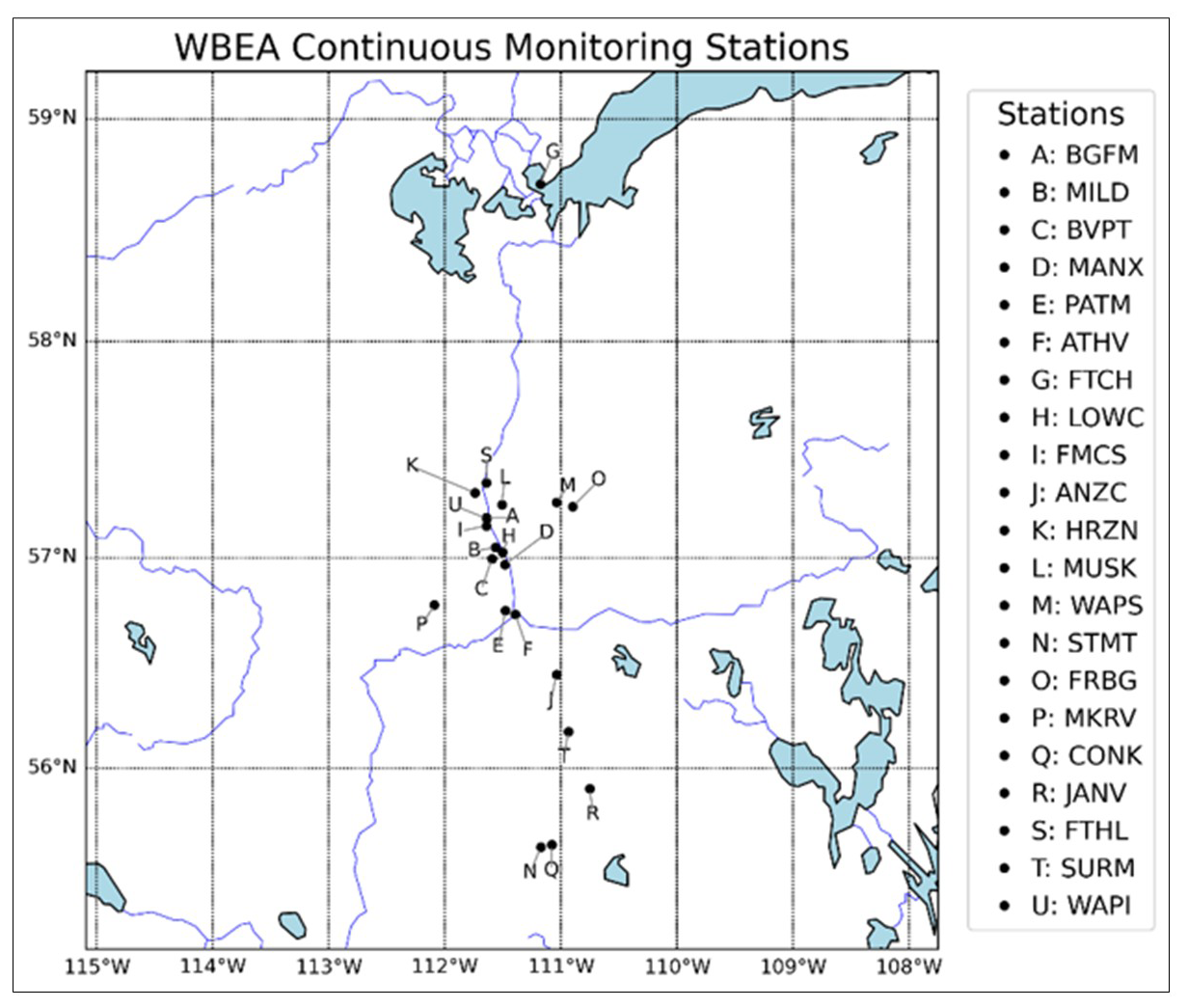
Figure 1 21 Wood Buffalo Environmental Association (WBEA) continuous monitoring stations with observations available during the period investigated in this work. These stations reported hourly (nearly continuous) observations of SO₂ in ppbv during this period.

3 Dry deposition algorithms

The dry deposition velocity (m s⁻¹) in GEM-MACH follows a “resistance model” approach (Erisman et al., 1994; Wesely, 1989; Baldocchi et al., 1987; Fowler, 1978; Wesely and Hicks, 1977; Garland, 1977), where the total deposition velocity for a grid cell is a land-use-fraction weighted sum, calculated as

$$\begin{array}{}\text{(1a)}& V_{{\mathrm{d}}_{\mathrm{gas}}}=\sum _{i=\mathrm{1}}^{\mathrm{nlus}}(v_{{\mathrm{d}}_i}\times f_i),\end{array}$$

where

$$\begin{array}{}\text{(1b)}& v_{{\mathrm{d}}_i}={\displaystyle \frac{\mathrm{1}}{r_{\mathrm{a}}+r_{\mathrm{b}}+r_{\mathrm{c}}}}.\end{array}$$

In Eq. (1a), f_i is the fractional land use (0.0 to 1.0) of land use type i (with a total of nlus land use categories). r_a is the gas-independent aerodynamic resistance between height z_r and the surface, r_b is the quasi-laminar sublayer resistance and r_c is the bulk surface resistance. The aerodynamic resistance depends on meteorological and land surface characteristics, while the r_b and r_c terms also depend on the gas being deposited. All resistance “r” terms have units of s m⁻¹. In GEM-MACH, the parametrization described in Wesely (1989) is used to calculate the bulk surface resistance r_c:

$$\begin{array}{}\text{(2)}& r_{\mathrm{c}}={\displaystyle \frac{\mathrm{1}}{\frac{\mathrm{1}-W_{\mathrm{st}}}{r_{\mathrm{s}}+r_{\mathrm{m}}}+\frac{\mathrm{1}}{r_{{\mathrm{cut}}_{\mathrm{zha}}}}+\frac{\mathrm{1}}{r_{\mathrm{conv}}+r_{\exp }}+\frac{\mathrm{1}}{r_{\mathrm{ac}}+r_{\mathrm{g}}}}},\end{array}$$

where r_m is the mesophyll resistance, r_s is the stomatal resistance with W_st=0 for no stomatal blockage and W_st=0.5 to account for the partial blockage of the stomata by water during precipitation and at high ambient relative humidity. r_cut is the leaf cuticular resistance, r_conv is the resistance of gas-phase transfer due to buoyant convection, r_exp is the resistance of leaves, twigs, bark and other exposed surfaces in the lower canopy (including buildings), r_ac is the in-canopy aerodynamic resistance (which depends on the canopy height and the canopy density) and r_g is the ground (soil) resistance. Details of the terms in the deposition algorithm are provided in the Supplement, Sect. S1.0. Three terms however include a dependence on the surface concentration of the hydrogen ion, through effective Henry's Law constants: r_m, r_cut, and r_exp: The formulae for these terms are, respectively (Makar et al., 2018; Clifton et al., 2023),

$$\begin{array}{}\text{(3)}& {\displaystyle }{r}_{\mathrm{m}}={\displaystyle \frac{\mathrm{1}}{\mathrm{LAI}\left(\frac{H_{\mathrm{sp}}^{\ast }}{\mathrm{3000}}+\mathrm{100}{x}_{{\mathrm{0}}_{\mathrm{sp}}}\right)}},\text{(4)}& {\displaystyle }{r}_{{\mathrm{cut}}_{\mathrm{zha}}}={\displaystyle \frac{r_{{\mathrm{cut}}_{\mathrm{0}}}}{\frac{H_{\mathrm{sp}}^{\ast }}{{\mathrm{10}}^{\mathrm{5}}}+x_{{\mathrm{0}}_{\mathrm{sp}}}}},\end{array}$$

and

$$\begin{array}{}\text{(5)}& r_{\exp }={\displaystyle \frac{\mathrm{1}}{\frac{H_{\mathrm{sp}}^{\ast }}{{\mathrm{10}}^{\mathrm{5}}{r}_{\exp ,{\mathrm{SO}}_{\mathrm{2}}}}+\frac{x_{{\mathrm{0}}_{\mathrm{sp}}}}{r_{\exp ,{\mathrm{O}}_{\mathrm{3}}}}}}.\end{array}$$

In these formulae, LAI is the single-sided leaf area index (m² leaf area per m² ground area), and the relative surface reactivity term $x_{{\mathrm{0}}_{\mathrm{sp}}}$ has been parameterized using half-redox potentials outlined in Zhang et al. (2002). $H_{\mathrm{sp}}^{\ast }$ is the species (sp) – dependent effective Henry's law constant, and $r_{\exp ,{\mathrm{SO}}_{\mathrm{2}}}$ and $r_{\exp ,{\mathrm{O}}_{\mathrm{3}}}$ are parameterized resistances which depend on the land use type.

Wesely's formulations for the cuticle, mesophyll, lower canopy and ground surface resistances all incorporate “parallel” resistance pathways for the removal of gases at each of these depositing surfaces via two chemical processes: (1) dissolution of soluble species, and (2) reactive destruction at the surface (making use of a chemical species-dependent parameter x₀). Wesely (1989) recognized that most direct observations of gas deposition fluxes are for the gases SO₂ and O₃ – the former being strongly influenced by the surface dissolution pathway, while the latter by the surface reactive destruction pathway. Hence the cuticle, mesophyll, lower canopy and ground surface resistance terms make use of ratios of the depositing specie's $H_{\mathrm{sp}}^{\ast }$ to that of SO₂, and x₀ is usually expressed to give a relative surface reactivity relative to that of O₃. Thus, in the Wesely formulation of r_c adopted in the GEM-MACH air quality model (Makar et al., 2018), $H_{\mathrm{sp}}^{\ast }$ is used in the terms describing r_m, $r_{{\mathrm{cut}}_{\mathrm{zha}}}$ and r_exp to “scale the rates of uptake by moist and wet surfaces relative to rates for SO₂ uptake” (Wesely, 1989). This scaling relative to SO₂ is the reason for division of $H_{\mathrm{sp}}^{\ast }$ by 10⁵ in the above formulae for $r_{{\mathrm{cut}}_{\mathrm{zha}}}$ and r_exp, because for neutral conditions $H_{\mathrm{sp}}^{\ast }$ for SO₂ ($H_{{\mathrm{SO}}_{\mathrm{2}}}^{\ast }$, where $H_{{\mathrm{SO}}_{{\mathrm{2}}_{\mathrm{neutral}}}}^{\ast }=H_{{\mathrm{SO}}_{{\mathrm{2}}_n}}^{\ast })\approx {\mathrm{10}}^{\mathrm{5}}$ M atm⁻¹; near-neutral conditions are presumed to be typical of water in plant sap and in the substomatal cavities of the leaves (Wesely, 1989). $H_{\mathrm{sp}}^{\ast }$ for chemical species which dissociate are usually functions of the concentration of hydrogen ions in the solution.

The formulae describing the [H⁺] dependence on H^∗ for key gas species are given in Table S1 in the Supplement, while other parameters for the deposition velocity calculations are provided in Table S2. $H_{\mathrm{sp}}^{\ast }$ for dissociating species will have a first or second-order inverse dependence on the hydrogen ion concentration (that is, $H_{\mathrm{sp}}^{\ast }\left(\left[{\mathrm{H}}^{+}\right]\right)\propto {\left[{\mathrm{H}}^{+}\right]}^{-\mathrm{1}}$ for a single dissociation stage, while species with two levels of dissociation will also have $H_{\mathrm{sp}}^{\ast }\left(\left[{\mathrm{H}}^{+}\right]\right)\propto {\left[{\mathrm{H}}^{+}\right]}^{-\mathrm{2}})$. Noting that $\mathrm{pH}=-{\log }_{\mathrm{10}}\left[{\mathrm{H}}^{+}\right]$, increases in pH (i.e. decreases in [H⁺]) will lead to increases in $H_{\mathrm{sp}}^{\ast }$, and hence resulting in decreases in the mesophyll, cuticle and lower canopy resistances (Eqs. 3–5), leading potentially to decreases in the surface resistance r_c (Eq. 2) and thus increases in the deposition velocity (Eq. 1).

A key point of the work described herein is that past work such as Wesely (1989) and many subsequent models use a constant value of $H_{\mathrm{sp}}^{\ast }$ or its equivalent metric, usually taken to represent a “neutral” solution at the surface of the different vegetation components as described in the earlier equations. In contrast, some chemical transport models employed an approach to use “climatological” soil pH categories indicated from geophysical data as the basis for changing the reference values of $r_{\mathrm{g},{\mathrm{SO}}_{\mathrm{2}}}$ spatially across the land surface (Ganzeveld et al., 1998; Kerkweg et al., 2006, 2009). However, the leaf surface pH may be perturbed quite dynamically by the recent deposition history of all depositing species, implying potentially higher or lower deposition conductances or net deposition velocities than predicted by assuming neutral conditions. To obtain $H_{\mathrm{sp}}^{\ast }$ for SO₂ as used in Wesely (1989) and Zhang et al. (2002), the solution pH of the surface must be 6.59, i.e., $\left[{\mathrm{H}}^{+}\right]=\mathrm{2.57}\times {\mathrm{10}}^{-\mathrm{7}}$ M, using the formula in Table S1 at a standard ambient temperature of 298 K. In this case, when $H_{{\mathrm{SO}}_{\mathrm{2}}}^{\ast }>H_{{\mathrm{SO}}_{{\mathrm{2}}_n}}^{\ast }$ (i.e., pH > 6.59) the impact of the $\frac{H_{\mathrm{sp}}^{\ast }}{{\mathrm{10}}^{\mathrm{5}}}$ term is to reduce the cuticular resistance ($r_{{\mathrm{cut}}_{\mathrm{zha}}}$), thereby decreasing the bulk surface resistance (r_c) and increasing the deposition velocity of SO₂ ($V_{{\mathrm{d}}_{{\mathrm{SO}}_{\mathrm{2}}}}$). The converse is true when $H_{{\mathrm{SO}}_{\mathrm{2}}}^{\ast }<H_{{\mathrm{SO}}_{{\mathrm{2}}_n}}^{\ast }$ (pH < 6.59) with an increase in r_c and hence a decrease in $V_{{\mathrm{d}}_{{\mathrm{SO}}_{\mathrm{2}}}}$. Thus, by allowing $H_{\mathrm{sp}}^{\ast }$ to vary with surface pH rather than assuming a neutral value, we see from the formulae of Table S1 that solution pH (i.e., within a water layer on a leaf surface) can directly impact the deposition of soluble gas species which dissociate or hydrate upon dissolution to give off H⁺, such as SO₂, HNO₃, HONO and NH₃. The linear dependence of the reactive gas uptake rate on $H_{\mathrm{sp}}^{\ast }$ was demonstrated in a formulation of multiphase chemical interactions between air and leaf-surface dew water by Chameides (1987) (see their Eqs. 14, 15, and 18) for a highly conceptual process-oriented study, where additional factors such as the chemical loss rate for depositing compounds within the dew, the total volume of dew water and its growth or shrinkage rate were also shown to control the gas uptake kinetics. Non-linearity in how these additional factors synergistically contribute to the rate of the gas uptake, hence the conductance for the gas deposition on the leaf surface, etc., is missing in the resistance formulations such as for $r_{{\mathrm{cut}}_{\mathrm{zha}}}$ in Eq. (4) despite allowance being made for the serial addition of the chemical reactivity term ($x_{{\mathrm{0}}_{\mathrm{sp}}}$) and will be a subject of our potential future studies.

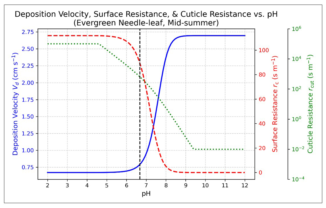
Figure 2 The variation in the deposition velocity (V_d, cm s⁻¹), bulk surface resistance (r_c, s m⁻¹) and the cuticular resistance (r_cut, s m⁻¹) of SO₂ as a function of foliage pH, calculated using the equation for $H_{{\mathrm{SO}}_{\mathrm{2}}}^{\ast }$ given in Table S1. The land use type was selected as an evergreen needleleaf forest in mid-summer, with an LAI = 3.5, $u_{\ast }=\mathrm{0.6}$ m s⁻¹, L=250 m, Q_p=450 W m⁻², T=22 °C, RH=62 % and [CO₂] = 425 ppm, representative of the AOSR during this time of year (Hayden et al., 2021). The black dashed line indicates a pH = 6.68, which is the current “near-neutral” pH assumed in GEM-MACH calculations of $H_{{\mathrm{SO}}_{\mathrm{2}}}^{\ast }$.

The “solution pH effect” is demonstrated for SO₂ in Fig. 2, for the GEM-MACH “evergreen needleleaf forest” land use category in mid-summer, using an LAI = 3.5, $u_{\ast }=\mathrm{0.6}$ m s⁻¹, a Monin–Obukhov length L=250 m, Q_p = 450 W m⁻², T=22 °C, RH = 62 % and [CO₂] = 425 ppm. These values are representative of mid-summer AOSR conditions (Hayden et al., 2021). Immediately obvious from Fig. 2 is the rapid variation in V_d with a unit change in the foliage pH; an increase in the pH from 7.0 to 8.0 increases V_d from about 1.0 to 2.4 cm s⁻¹, an increase of 140 % or a factor of 2.4×. The pH impact on $r_{{\mathrm{cut}}_{\mathrm{zha}}}$ (and hence V_d) is largely confined to the range between pH = 5.0 and pH = 9.0. Below pH = 5.0 and above pH = 9.0, r_c reaches an asymptote, regardless of whether $r_{{\mathrm{cut}}_{\mathrm{zha}}}$ is further increased or decreased respectively. Hence in this study, $r_{{\mathrm{cut}}_{\mathrm{zha}}}$ is bounded within the range between 0.01 and 99 999.9 s m⁻¹; for comparison this lower limit of 0.01 s m⁻¹ for $r_{{\mathrm{cut}}_{\mathrm{zha}}}$ is 2000 times smaller than the lower limit of 20 s m⁻¹ suggested by Zhang et al. (2002) (see Sect. 5.2).

4 Simulating foliage pH: Modifications to the dry deposition algorithm

Several considerations must be addressed in order to carry out the calculation of foliage pH for the purposes of deposition velocity estimation, in addition to incorporating the dependence of V_d on [H⁺], as described in Sect. 3. Choices must be made regarding which foliage types should be subject to pH-dependent deposition. The accumulation of previously deposited material must be tracked across time steps (since this will determine the pH of the foliage surface in the current time step). This tracking must include both deposition fluxes to the foliage and the removal of deposited material via precipitation (washoff). The amount of liquid water adhering to leaf surfaces must also be estimated, from both meteorological and thermodynamic sources. The pH calculation must take into account high-concentration thermodynamic chemistry, since the water amounts can be sufficiently small that non-ideal solution chemistry solvers must be employed. The formula representing deposition must make use of the resulting pH values, and account for varying types of foliage within each model grid cell; the extent to which deposition specifically to the foliage portion of the surface is resolved may depend on the algorithm (for example, the gas and particle deposition algorithms may differ in this respect). These aspects of the simulation of foliage pH are discussed in Sect. 4.1 through 4.5. Note that none of the pH calculations are employed in the Base Case simulations, which use the default pH value of 6.68.

4.1 Restricting the pH dependence to “Natural Vegetation”

In the GEM-MACH model, the deposition of a gaseous species to foliage has two main pathways: (1) to the leaf surface (leaf cuticle) and (2) to the leaf interior (trans-cuticular and stomatal deposition). The relative importance of the different pathways may depend on both the vegetation type and the identity of the gas. In this investigation, the fraction of gaseous deposition that occurs to the leaf surface in a grid cell is estimated via effective conductances for each land-use type containing “natural vegetation”. While GEM-MACH has 15 unique land-use types for dry deposition modelling, only 4 of these are considered in our high resolution foliage pH co-deposition simulations, including: (1) evergreen needleleaf forests, (2) deciduous broadleaf forests, (3) mixed forests and (4) dwarf trees and shrubs (Fig. 3). Vegetation classes containing grassland or crops were not considered since these types of vegetation may have non-trivial anthropogenic interventions at the leaf foliage level (i.e., fertilizer application, harvesting, pruning), thus generating a large uncertainty in the deposition accumulators, and as a result, the predicted foliage pH. In all cases, deposition accumulation (and pH calculation) is only considered for forest canopies with canopy heights h_c>1 m, but in almost all cases h_c is well above this limiting value for the selected vegetation classes.

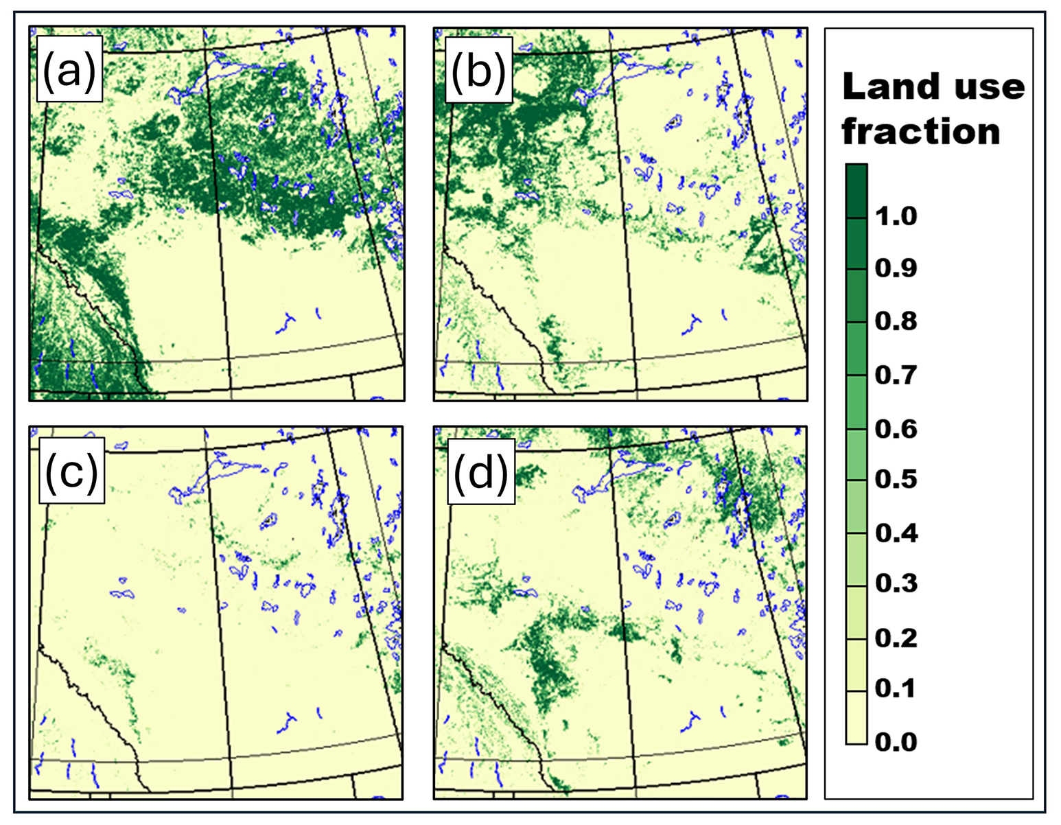
Figure 3 Land use fractions (0.0–1.0) for vegetation classes in GEM-MACH simulations: (a) evergreen needleleaf forests, (b) deciduous broadleaf trees, (c) mixed wood forests and (d) dwarf trees, shrubs with ground cover. While GEM-MACH contains classes for evergreen broadleaf and deciduous needleleaf forests, the land-use fraction for these categories is 0.0 in the entire geographic domain investigated here.

4.2 Comparison of resistances: cuticle resistance as the main pathway for pH dependence

The cuticle resistance pathway is the only pathway present in the Wesely parameterization wherein an H^∗ dependent term critically controls the entire pathway's contribution to the deposition flux. For example, the mesophyll pathway, which also includes an H^∗ dependence, is already characterized by a very low resistance for the mesophyll portion, consistent with observations that show the stomatal resistance is the dominant barrier to SO₂ assimilation (Pfanz et al., 1987). The mesophyll resistance is added in series to the stomatal resistance, and the latter lacks an H^∗ dependence. The net deposition flux via the overall stomatal pathway is determined largely by the stomatal resistance itself, and consequently the influence of H^∗ on the combined pathway is likely to be small. Furthermore, the mesophyll pH, representative of the apoplastic fluid within the leaf, remains relatively constant at a neutral to slightly acidic pH, making the use of a constant H^∗ in this term more appropriate (Yu et al., 2000; Savchenko et al., 2000). For the soil pathway, the r_ac term adds in series with the r_g term, the former of which is not dependent on H^∗ in the above formulation. Since typically r_ac≫r_g for the forest categories of the land-use type, the H^∗ term has a minor influence on the soil pathway. The lower canopy (r_exp) term's H^∗ dependence, coupled with the low value of r_conv, implies it may be a candidate pathway for an H^∗ dependence. However, the relatively high values of the $r_{\exp ,{\mathrm{SO}}_{\mathrm{2}}}$ and $r_{\exp ,{\mathrm{O}}_{\mathrm{3}}}$ coefficients ensure that this overall pathway has relatively little mass flux (and is often left out of deposition algorithms altogether). In contrast, the cuticle pathway's H^∗ dependence is capable of controlling (and greatly reducing) the cuticle resistance without interferences from additional resistances acting directly within this pathway and hence may have a significant impact on the resulting deposition velocity. We therefore focus specifically on the pH influence on the cuticle pathway, in our work that follows.

4.3 Accumulation of Deposition Fluxes

From the above development, a requirement for calculating cuticle surface pH is the need to track and accumulate the past history of that portion of the deposition flux which ends up on the cuticles of natural vegetation foliage. This calculation is specific to the deposition algorithm employed: Eqs. (6), (7) and (8), below, and their theoretical development in the Supplement (Sects. S2.0 and S3.0), are specific to GEM-MACH's deposition algorithms, but the methodology employed is generalizable to any deposition algorithm.

4.3.1 Accumulating the flux of gases to cuticle surfaces

The potential impact of changes to the H^∗ value associated with gaseous deposition via the cuticle pathway requires that an estimate be made of the deposition flux via that pathway. This was done by using the concept of effective fluxes (Galmarini et al., 2021). The Supplement (Sects. S2.0 and S3.0) describes the development of the terms for the portion of the deposition flux which is associated with both the cuticle resistance and the natural vegetation types as per Fig. 3. Note that the formulae are specific to the gas deposition algorithm used in GEM-MACH, but the same methodology may be applied to other deposition algorithms using the effective conductance formulation specific to that algorithm, as outlined in the Supplement, Sects. S2.0 and S3.0. Here we state the final resulting formulae.

For gases other than ammonia, the deposition flux to vegetation cuticles on the leaf surfaces of natural vegetation for the jth gas is given by:

$$\begin{array}{}\text{(6)}& F_{{\mathrm{cut}}_j}={\displaystyle \frac{\begin{array}{c}{\sum }_{i=\mathrm{1}}^{\mathrm{nlus}}[v_{{\mathrm{d}}_{j,i}}\times f_i\times {\mathit{\delta }}_i\\ \left.\times \left(\frac{\frac{\mathrm{1}}{r_{{\mathrm{cut}}_{j,i}}}}{\frac{\mathrm{1}-W_{\mathrm{st}}}{r_{{\mathrm{s}}_{j,i}}+r_{{\mathrm{m}}_{j,i}}}+\frac{\mathrm{1}}{r_{{\mathrm{cut}}_{j,i}}}+\frac{\mathrm{1}}{r_{{\exp }_{j,i}}+r_{{\mathrm{conv}}_{j,i}}}+\frac{\mathrm{1}}{r_{{\mathrm{ac}}_{j,i}}+r_{{\mathrm{g}}_{j,i}}}}\right)\right]\end{array}}{\sum _{i=\mathrm{1}}^{\mathrm{nlus}}(v_{{\mathrm{d}}_{j,i}}\times f_i)}}\times F_j\end{array}$$

Where j,i indicates the jth gas and the ith land-use type, f_i is the fractional area comprised of land-use type i within a given grid cell, F_j is the total flux, and δ_i=1 when the land-use type is one in which the pH dependence is to be calculated, and δ_i=0 otherwise.

Gases with bidirectional fluxes such as ammonia (NH₃) require a treatment that depends on the bidirectional flux algorithm employed. In the case of the bidirectional NH₃ flux algorithm employed in GEM-MACH (Zhang et al., 2010), the NH₃ flux through the cuticle pathway is always downward, and depends on vegetation-and-meteorology-dependent canopy compensation point concentration of NH₃ ($x_{{\mathrm{c}}_{{\mathrm{NH}}_{\mathrm{3}}}}$, µg m⁻³), and on the cuticle resistance $r_{{\mathrm{cut}}_{{\mathrm{NH}}_{\mathrm{3}}}}$ (s m⁻¹); the cuticle flux in $F_{{\mathrm{cut}}_{{\mathrm{NH}}_{\mathrm{3}}}}$ (mol m⁻²) for a given land use type is given by:

$$\begin{array}{}\text{(7)}& F_{{\mathrm{cut}}_{{\mathrm{NH}}_{\mathrm{3}}}}={\displaystyle \frac{x_{c_{{\mathrm{NH}}_{\mathrm{3}}}}\times {\mathrm{10}}^{-\mathrm{6}}}{r_{{\mathrm{cut}}_{{\mathrm{NH}}_{\mathrm{3}}}}\times M_{{\mathrm{NH}}_{\mathrm{3}}}}}\times \mathrm{\Delta }t\end{array}$$

Equations (6) and (7) may be used to accumulate the fluxes of gases to cuticle surfaces, for later calculation of the cuticle surface pH.

4.3.2 Accumulating the flux of particle species to cuticle surfaces

The capture of particulate matter by vegetation is highly dependent on both particle and foliage specific traits. Foliage surface area, pubescence (i.e., leaf hairs) and roughness (i.e., grooves, ridges, folds) can all impact the retention of particles by vegetation, with each trait being highly specific to the vegetation species (see Sect. 1). Regional air quality models cannot resolve these foliage-specific factors, and hence simplified parameterizations are applied to estimate deposition of particles to vegetation. For particulate species, dry deposition in a vegetated area may occur to the plant surface (i.e., leaves, bark) or to the ground. Unlike the algorithm for gases, the deposition algorithm for particles in GEM-MACH does not explicitly separate between these individual pathways but instead employs a parameterized particle-size-dependent “surface collection efficiency” (ε_i,k) to represent the fraction of particles of size range k that are collected by any canopy and surface elements (leaves, soil, etc.) on the land-use type i. The particle flux specifically to cuticles must be estimated using the available information (Supplement, Sect. S3.0). Here we provide the final result for $F_{{\mathrm{cut}}_{\mathrm{sp}}}$, the net flux of particulate species sp to cuticle surfaces for natural vegetation:

$$\begin{array}{}\text{(8)}& \begin{array}{rl}{F}_{{\mathrm{cut}}_{\mathrm{sp}}}& =\left({\displaystyle \frac{\mathrm{LAI}}{\mathrm{LAI}+\mathrm{1.0}}}\right)\\ & \times \sum _{k=\mathrm{1}}^{n_{\mathrm{size}}}\left[\left({\displaystyle \frac{\sum _{i=\mathrm{1}}^{\mathrm{nlus}}\left[{\mathit{\delta }}_i\times f_i\times v_{{\mathrm{d}}_{i,k}}\right]}{\sum _{i=\mathrm{1}}^{\mathrm{nlus}}\left[f_i\times v_{{\mathrm{d}}_{i,k}}\right]}}\right)\times F_{\mathrm{sp},k}\right]\end{array}\end{array}$$

Where f_i and δ_i are defined as for Eq. (6) above, LAI is the leaf area index for the grid cell, $v_{{\mathrm{d}}_{i,k}}$ is the deposition velocity of particles of size k for land-use type i, and F_sp,k is the total flux of particulate species sp for particle size k.

Equation (8) may be used to accumulate the flux of particulate species to cuticle surfaces, needed for the calculation of cuticle surface pH.

4.4 Removal of mass on foliage surfaces by precipitation

Particles deposited onto the leaf surface can be removed from the foliage surface by precipitation, a process referred to as washoff. The precipitation may dissolve solid soluble particles forming an aqueous solution or physically dislodge insoluble particles captured in the grooves or by the hairs of the leaf (Sect. 1). The net result is a reduction in the particle mass on the leaf surface. Experimental investigations into washoff under controlled conditions have shown that the cumulative precipitation amount is the dominant factor determining how much mass is removed from the leaf (Fortmann and Johnson, 1984; Potter and Ragsdale, 1991; Pullman, 2009; Xu et al., 2019). Potter and Ragsdale (1991) investigated the removal of SO${}_{\mathrm{4}}^{\mathrm{2}-}$ and K⁺ ions by precipitation from freshly collected broadleaf forest species in North Carolina (Acer rubrum L., Quercus prinus L., Cornus florida L., and Rhododendron maximum L.) using sequential simulated rainfall events. Their results showed that sulphate removal approached zero after 8 to 11 mm of precipitation, suggesting complete removal of soluble material is possible. Pullman (2009) similarly studied the washoff of applied KNO₃ particles from coniferous needles (Pinus strobus, Taxus cuspidate and Tsuga canadensis) and found that 70 % to 90 % of deposited mass was removed after 18.5 mm of simulated rainfall. To parameterize the washoff, Pullman (2009) suggested the function

$$\begin{array}{}\text{(9)}& R\left(P\right)=y_{\mathrm{0}}+a{e}^{-bP},\end{array}$$

where R(P) is the remaining fraction of surface mass after cumulative precipitation P (in mm) and y₀, a and b are observation-based fitted constants. In Pullman (2009), the fitted y₀ value is nonzero, suggesting some residual mass is retained even after extensive precipitation – potentially due to insoluble material or mechanical retention within leaf structures. In this work, we adopt a simplified approach based on the sulphate data reported in Potter and Ragsdale (1991), where it is assumed that all particle species are fully soluble and subject to complete washoff with sufficient precipitation. Accordingly, we set y₀=0, a=1 and determine $B=\mathrm{0.189}\pm \mathrm{0.032}$ via least-squares regression of the Potter and Ragsdale (1991) sulphate washoff measurements. The least squares regression is shown in Fig. 4 as a dashed line. This simplification assumes that all modelled particulate matter is readily water-soluble, representing a significant source of uncertainty and a likely oversimplification, especially for modelling the washoff of insoluble or the partially soluble part of material deposited on leaf surfaces (see Sects. 4.4 and 6.0). Nonetheless, we believe that it is not a major drawback for this study because our primary purpose is the simulation of pH in the hygroscopic material.

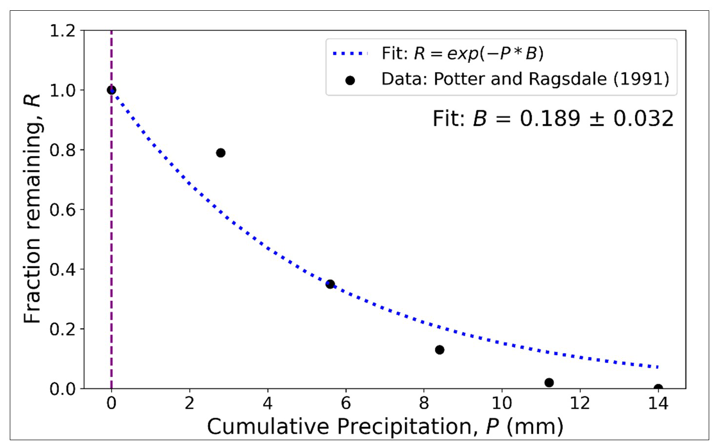
Figure 4 Linear least squares best fit of $R=\exp \left(-P\times B\right)$, where R is the fraction of mass remaining on the leaf after P mm of cumulative rainfall. The fitting parameter B is estimated to be 0.189 ± 0.032. Data were obtained by interpolating data presented graphically in Potter and Ragsdale (1991).

Since GEM-MACH is a timestep based model, it is necessary to determine the washoff that would occur over the timestep Δt. For each rainfall event, this requires tracking of (1) the concentration of each species (gas and particle) in the canopy volume at the commencement of the rainfall (M_init), and (2) the cumulative precipitation (P) at the current (i) and previous (i−1) timestep. Here the cumulative precipitation is tracked per timestep per rainfall event. Over timestep Δt where q mm of rainfall occurs ($P_i=P_{i-\mathrm{1}}+q$), the mass of a deposited soluble species removed from the canopy volume after a timestep of precipitation (WO_t) is modelled as

$$\begin{array}{}\text{(10)}& {\mathrm{WO}}_t={\mathrm{WO}}_{t-\mathrm{1}}\left[e^{-b{P}_{i-\mathrm{1}}}-e^{-b{P}_i}\right].\end{array}$$

It should be noted that dry deposition is not accumulated on the leaf surface during precipitation events, and thus during precipitation events only removal is considered. Furthermore, a lower concentration limit of $\mathrm{1.0}\times {\mathrm{10}}^{-\mathrm{20}}$ mol m⁻³ is used in the case of complete removal, to avoid division by zero.

4.5 Estimating Water on Foliage Surfaces: the importance of the lower threshold for layer thickness

An important requirement in calculating cuticle surface pH is an accurate estimate of the amount of water residing on the leaf surface. The quantity of liquid water retained on the leaf, defined here in terms of the leaf water layer thickness, crucially affects the leaf water layer pH (Burkhardt and Eiden, 1990; Chameides, 1987; Klemm et al., 1987). Chemical thermodynamics solvers such as HETP (see Sect. 4.6.1) predict foliage water that would result from aerosol deliquescence, but additional water may be present on the foliage due to meteorological conditions such as rain, dew, fog and leaf guttation (the secretion of plant water from foliage). These additional water inputs were not considered in the original HETP calculations, and if present, neglecting these additional sources of water would result in a bulk leaf water solution that is too concentrated. However, the GEM weather forecast model (upon which the GEM-MACH air-quality model is based) simulates rainfall and dew water intercepted by the canopy in its physical parameterization based on the ISBA (Interactions between Soil, Biosphere and Atmosphere) land surface scheme, providing an estimate of the canopy water content w_r (kg m⁻² ground area) (Bélair et al., 2003a, b), hereafter referred to as “meteorological water”. We convert this w_r to a bulk canopy-level estimate (kg m⁻³ of canopy volume) by dividing by the canopy height as

$$\begin{array}{}\text{(11)}& W_{\mathrm{met}}={\displaystyle \frac{w_{\mathrm{r}}}{h_{\mathrm{c}}}}.\end{array}$$

In this work, HETP has been modified to accept the meteorological water W_met as an input at the start of the thermodynamic calculations used in cuticle surface pH estimation. W_met remains constant during the iterative process within HETP to determine [H⁺] – hence this additional non-aerosol water is allowed to perturb the thermodynamic equilibrium. In addition to W_met predicted by the GEM weather model, HETP may increase the total foliage water by an amount determined from aerosol deliquescence (W_aero). W_aero is not accounted for in W_met, since the ISBA parameterization used in GEM does not consider aerosol deliquescence (Bélair et al., 2003a, b). Since it is often the case that W_met≫W_aero, W_aero becomes important only during times when W_met≈0. Upon the exit of its process calculations, HETP provides the total foliage water (W_tot) with units of kg m⁻³ of canopy volume, calculated as the sum of W_met (unchanged) and W_aero, that is, $W_{\mathrm{tot}}=W_{\mathrm{met}}+W_{\mathrm{aero}}$. W_tot is then used in conjunction with $\left[{\mathrm{H}}_{\mathrm{air}}^{+}\right]$ (with units of mol m⁻³) to estimate a bulk foliage pH as

$$\begin{array}{}\text{(12)}& {\mathrm{pH}}_{\mathrm{leaf}}=-{\log }_{\mathrm{10}}\left({\displaystyle \frac{\left[{\mathrm{H}}_{\mathrm{air}}^{+}\right]}{W_{\mathrm{tot}}\times \frac{\mathrm{1}\mathrm{L}}{\mathrm{1}\mathrm{kg}}}}\right)\end{array}$$

From W_tot, a leaf-level bulk estimate of the water layer thickness (in µm) is calculated¹ as

$$\begin{array}{}\text{(13)}& L_{\mathrm{w}}=\mathrm{1000}{W}_{\mathrm{tot}}{h}_{\mathrm{c}}/\left(\mathrm{2}\mathrm{LAI}\right).\end{array}$$

pH_leaf is only calculated if L_w is greater than or equal to a threshold value $L_{{\mathrm{w}}_{\mathrm{Thres}}}$. If $L_{\mathrm{w}}<L_{{\mathrm{w}}_{\mathrm{Thres}}}$, that is, the water layer thickness falls below the threshold value, we assume that pH_leaf has a neutral value of 6.68. This threshold on L_w is also physically necessary in that at sufficiently low surface concentrations, water is unlikely to form a contiguous layer.

Previous studies have estimated microscopic water layers on foliage surfaces to typically be in the range of 0.05 to 5 µm (Burkhardt and Hunsche, 2013; Van Hove et al., 1989; Sutton et al., 1998), while some studies have suggested the possibility of much thinner water layers, between 1 and 4 nm (Adema and Heeres, 1995; Burkhardt and Eiden, 1994; Burkhardt and Eiden, 1990). To investigate the impact of the choice of the $L_{{\mathrm{w}}_{\mathrm{Thres}}}$ on the resulting dry deposition velocities of SO₂, two thresholds were investigated: $\mathrm{5}\times {\mathrm{10}}^{-\mathrm{4}}$ and 0.1 µm. We investigated the impact of these alternative values of $L_{{\mathrm{w}}_{\mathrm{Thres}}}$ on resulting pH estimates in multi-month simulations on a North American domain (see Fig. S2 in the Supplement): the lower threshold resulted in unrealistically extreme pH values, either very acidic (pH < 2) or very basic (pH > 10). The higher threshold also resulted in better performance in comparison with surface SO₂ observations in the relatively dry month of May. In that month, foliage water layers are often sustained only by aerosol deliquescence (W_aero), resulting in very high ionic strength. Under these conditions, simulations employing the higher water layer threshold and hence lower ionic strength) had better statistical agreement with observations than those with the lower threshold. Hence in the sections that follow, we employ $L_{{\mathrm{w}}_{\mathrm{Thres}}}=\mathrm{0.1}$ µm.

4.6 Foliage pH calculations

4.6.1 Initial pH calculation: HETP

The foliage pH is first estimated from the Heterogeneous Vectorized or Parallel (HETP) model of chemical thermodynamics (Miller et al., 2024), using the concentrations of accumulated gases and particles in the canopy volume, and the occurrence of precipitation as inputs, as well as the foliage water predicted by the GEM meteorological model. HETP was selected for this purpose since it includes the computation of activity coefficients in its prediction of pH, which is important for dealing with “non-ideal” solutions; those with high ionic strength expected to occur under subsaturated humidity conditions on the cuticle surface.

In order to estimate pH, we first convert the accumulation of timestep atmospheric deposition $F_{{\mathrm{cut}}_{\mathrm{gas}}}$ and $F_{{\mathrm{cut}}_{\mathrm{sp}}}$ subsequent to the last precipitation event at each timestep to a bulk canopy “concentration” with units of mol m⁻³ of canopy volume by dividing by the canopy height h_c (m) as

$$\begin{array}{}\text{(14)}& G_{{\mathrm{sp}}_{\mathrm{cut}}}={\displaystyle \frac{F_{{\mathrm{cut}}_{\mathrm{gas}}}}{h_{\mathrm{c}}}}\end{array}$$

and

$$\begin{array}{}\text{(15)}& P_{{\mathrm{sp}}_{\mathrm{cut}}}={\displaystyle \frac{F_{{\mathrm{cut}}_{\mathrm{sp}}}}{h_{\mathrm{c}}}}.\end{array}$$

This simplification assumes that the deposited mass (and predicted foliage water) is evenly distributed over the entire height of the canopy; this allows a calculation of the pH for the canopy to be made a “bulk” calculation, in analogy to the typical application of algorithms such as HETP to particle inorganic chemistry. $G_{{\mathrm{sp}}_{\mathrm{cut}}}$ and $P_{{\mathrm{sp}}_{\mathrm{cut}}}$ are accumulated over time, referred to hereafter as “deposition accumulators”, and denoted as $T_t^{\mathrm{gas}}$ and $T_t^{\mathrm{par}}$ at time t. In this study, the removal of mass from foliage surfaces (and a consequent reduction in $T_t^{\mathrm{gas}}$ and $T_t^{\mathrm{par}}$) occurs only through the dominant process of precipitation washoff (${\mathrm{WO}}_t^{\mathrm{sp}}$), although strong winds may also cause removal of particle mass (Sect. 1). Precipitation washoff, given a sufficient amount of precipitation occurring over a sufficient amount of time, is assumed to be complete for the deposited gases (${\mathrm{WO}}_t^{\mathrm{gas}}=T_{t-\mathrm{1}}^{\mathrm{gas}}$) and particle species (${\mathrm{WO}}_t^{\mathrm{par}}=T_{t-\mathrm{1}}^{\mathrm{par}}$). Note that washoff by precipitation occurs over time according to Eq. (10). Gases and particles deposited to the leaf are thus assumed to be completely soluble in an excess of water (except for CaSO₄, which has relatively low solubility and hence is assumed to remain on the leaf surfaces). In addition, no mass is accumulated on the leaf surfaces during rainfall ($G_{{\mathrm{sp}}_{\mathrm{cut}}}=P_{{\mathrm{sp}}_{\mathrm{cut}}}=\mathrm{0}$; all depositing mass is assumed to be removed during rainfall events), and as such, a contribution from wet deposition of soluble gases and ions is also ignored in the calculation of foliage pH. Thus, the total bulk concentration residing on the foliage due to dry deposition in a canopy volume at timestep t is simulated for gas species as

$$\begin{array}{}\text{(16)}& \begin{array}{rl}& T_t^{\mathrm{gas}}=T_{t-\mathrm{1}}^{\mathrm{gas}}+G_{{\mathrm{sp}}_{\mathrm{cut}}}-{\mathrm{WO}}_t^{\mathrm{gas}},\\ & \mathrm{where}\left\{\begin{array}{ll}{\mathrm{WO}}_t^{\mathrm{gas}},& \left(\text{Precipitation is occuring at time}t\right)\\ {\mathrm{WO}}_t^{\mathrm{gas}}=\mathrm{0},& \left(\text{Otherwise}\right)\end{array}\right.\end{array}\end{array}$$

and likewise for particle species

$$\begin{array}{}\text{(17)}& \begin{array}{rl}& T_t^{\mathrm{par}}=T_{t-\mathrm{1}}^{\mathrm{par}}+P_{{\mathrm{sp}}_{\mathrm{cut}}}-{\mathrm{WO}}_t^{\mathrm{par}},\\ & \mathrm{where}\left\{\begin{array}{ll}{\mathrm{WO}}_t^{\mathrm{par}},& \left(\text{Precipitation is occuring at time}t\right)\\ {\mathrm{WO}}_t^{\mathrm{par}}=\mathrm{0},& \left(\text{Otherwise}\right)\end{array}\right..\end{array}\end{array}$$

In our simulation of the foliage pH, only the inorganic soluble gases SO₂, HNO₃, HCl and NH₃ are included for gaseous deposition accumulators, while for particle species, SO${}_{\mathrm{4}}^{\mathrm{2}-}$, HSO${}_{\mathrm{4}}^{-}$, NO${}_{\mathrm{3}}^{-}$, NH${}_{\mathrm{4}}^{+}$, Na⁺, Cl⁻, Ca²⁺, Mg²⁺ and K⁺ are included. These deposition accumulators are then used to calculate the hydrogen ion concentration [H⁺] using HETP; note that HETP assumes a unity activity coefficient for H⁺. HETP requires as input the total gas + aerosol concentrations (mol m⁻³) of total sulphate, total nitrate, total ammonia and total chloride. These are defined as, respectively, TS = SO₂ + HSO${}_{\mathrm{4}}^{-}$ + SO${}_{\mathrm{4}}^{\mathrm{2}-}$, TN = HNO₃ + NO${}_{\mathrm{3}}^{-}$, TA = NH₃ + NH${}_{\mathrm{4}}^{+}$ and TCl = HCl + Cl⁻. Here, SO₂ is simply assumed to be oxidized to sulphate upon deposition on the leaf surface, which we note is potentially inaccurate as a process description in cases where the S(IV) oxidation is limited by the co-deposition of atmospheric oxidants such as H₂O₂ and O₃ (Chameides, 1987; Wesely et al., 1990), and/or where antioxidants exudated from inside the leaves as speculated for example by Fuentes et al. (1994) are so high as to compete with or dominate over S(IV) in the consumption of oxidants in the leaf-surface aqueous solution. In addition to the above-mentioned inputs, HETP also requires the relative humidity and air temperature. For these simulations, the relative humidity and air temperature are set to the value of the lowest model layer (i.e., screen level). Since these calculations are being done using “bulk” concentrations, this work does not consider a “leaf-level” relative humidity or temperature.

HETP in its original form (Miller et al., 2024) assumes a metastable state in all thermodynamic calculations, therefore the final speciation consists only of aqueous ions and gases (except for CaSO₄, which is assumed to be insoluble). Prior to performing thermodynamic calculations, HETP determines the mass of anions and cations that can partition into a set of atmospherically relevant salts. These salts are then assumed to completely deliquesce, forming the initial aqueous phase speciation that is then used to seek the equilibrium state of the chemical system. In this approach HETP does not consider any “excess” mass of base cations beyond that required for thermodynamic equilibrium. For example, if the leaf surface contains only sulphate (TS) and potassium (TK), the dominant salt in HETP is assumed to be K₂SO₄. The concentration is determined² as [K₂SO₄] = $min\left(\mathrm{TS},\mathrm{0.5}\mathrm{TK}\right)$, potentially giving an excess or “free” amount of potassium as $K_{\mathrm{free}}=\mathrm{TK}-\mathrm{2}\left[{\mathrm{K}}_{\mathrm{2}}{\mathrm{SO}}_{\mathrm{4}}\right]$ in cases where TS<0.5 K. This “free” amount is not used when solving for thermodynamic equilibrium and as a result, does not affect [H⁺] (solution pH) predicted by the original HETP. The initial [H⁺] calculated by HETP is thus that of the portion of the deposited mass which is in equilibrium with anions, but does not include the influence of any “leftover” (i.e. “free”) excess base cation mass. Consequently, the maximum pH simulated by the original HETP algorithm alone is near 7.5. The focus for algorithms such as HETP is to determine the equilibrium between inorganic gaseous and particulate matter, hence the “excess” mass remains in the particulate phase, since it does not change the particle mass through partitioning. In most cases, this excess mass of base cations is originally balanced by carbonate alkalinity from CO${}_{\mathrm{3}}^{\mathrm{2}-}$ and/or HCO${}_{\mathrm{3}}^{-}$, which are prone to titration and the release of gaseous CO₂ promptly via chemical processing of the PM towards its neutralization and acidification in the atmosphere (i.e., Chameides and Stelson, 1992; Dentener et al., 1996). This is a process often neglected in HETP and other models of aerosol chemical thermodynamics. However, in cases where a significant amount of excess base cation mass exists on the leaf surface, for example downwind of cement processing facilities (Darley, 1966), the pH of the leaf water layer can exceed 7.5, because the amount of excess base cations and carbonate alkalinity is most likely in far excess of that of co-deposition acids. In these cases, the CO${}_{\mathrm{3}}^{\mathrm{2}-}$ from dissociated salts (such as calcium carbonate CaCO₃) may hydrolyse in the leaf water layer to form OH⁻, thereby buffering the solution in alkaline conditions. A second adjustment to the initial [H⁺] calculated by HETP is therefore required. We investigated two different adjustments. The first made use of a simple charge balance, and the second employed high-concentration, non-ideal chemical equilibria (CALCCO3, Sect. 4.6.2). The use of a simple charge balance was found to frequently result in unrealistically high pH values (e.g. greater than 10), and poorly resolved pH in the crucial 7.5 to 9.0 range. The water layers on foliage surfaces are sufficiently thin that calculations consistent with high concentration solution chemistry are therefore required to accurately represent pH (Miller et al., 2024; Fountoukis and Nenes, 2007). We therefore recommend the use of CALCCO3 instead of a simple charge balance for leaf foliage pH calculations, and focus on the use of CALCCO3 hereafter.

4.6.2 Final pH calculation: Thermodynamic Adjustment (CALCCO3)

A rigorous thermodynamic adjustment algorithm, CALCCO3, was developed, which explicitly accounts for equilibrium solution chemistry with free ions associated with carbonate alkalinity, as a follow-on to the initial HETP calculation. CALCCO3 simulates the water layer pH by including additional thermodynamic equilibria for atmospheric CO₂ and carbonate salts not considered in HETP. In this adjustment any excess of Ca, K, Na or Mg from the initial HETP calculation is assumed to be matched with carbonate as CaCO₃, K₂CO₃, Na₂CO₃ and MgCO₃, respectively. The final [H⁺] estimate resulting from this adjustment considers the individual temperature-dependant thermodynamic equilibria with additional considerations for mass balance, solubility constraints and electroneutrality. The CALCCO3 adjustment is applied to recalculate the initial HETP-derived pH if (1) the free mass of either Ca, Mg, Na or K remaining after the HETP calculation exceeds $\mathrm{1}\times {\mathrm{10}}^{-\mathrm{10}}$ mol m⁻³ and (2) the amount of liquid water exceeds $\mathrm{1}\times {\mathrm{10}}^{-\mathrm{10}}$ kg m⁻³. Below the limit applied in (1) we assume there is an insufficient mass of base cations yielding a negligible effect on the foliage water pH; below the limit of (2) we assume is insufficient foliage water to generate a water layer with a thickness exceeding $L_{{\mathrm{w}}_{\mathrm{Thres}}}$. No consideration has been made for activity coefficients in CALCCO3, unlike the original HETP algorithms. The reaction system solved by the CALCCO3 algorithm, and the theoretical development of the governing equations, are provided in the Supplement, Sect. S4.0.

5 Results and Discussion

5.1 Simulation of foliage pH

The effect of $L_{{\mathrm{w}}_{\mathrm{Thres}}}$ on the predicted SO₂ deposition velocity via foliage water pH is demonstrated in Fig. 5, which shows predicted $V_{{\mathrm{d}}_{{\mathrm{SO}}_{\mathrm{2}}}}$ for our final configuration, “CALCCO3_Lw_high”, from the 2.5 km resolution model for May 2018. We highlight this month since it featured many dry periods where L_w became very small and is largely dominated by aerosol water W_aero – later months are wetter overall. To avoid skewing the data shown in Fig. 5, times when the pH = 6.68 are excluded: a pH = 6.68 is used as the “reset” pH applied during times of insufficient foliage water, or in regions where there is insufficient natural vegetation (i.e., crops). The panels of Fig. 5 thus show model results when the thin water layer threshold of 0.1 µm has been exceeded in each case.

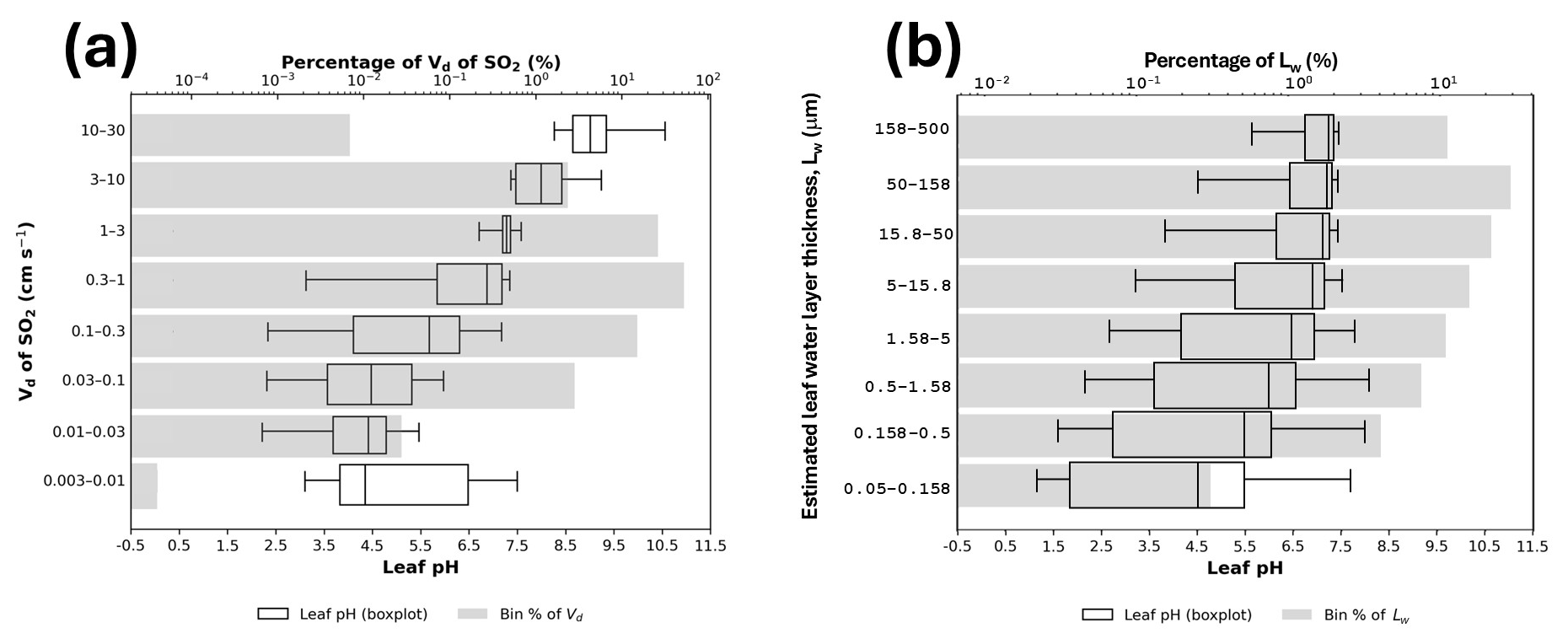
Figure 5 (a) The deposition velocity of SO₂ ($V_{{\mathrm{d}}_{{\mathrm{SO}}_{\mathrm{2}}}}$, cm s⁻¹) as a function of foliage (leaf) pH; data are from May 2018. $V_{{\mathrm{d}}_{{\mathrm{SO}}_{\mathrm{2}}}}$ has been separated into 8 discrete bins, and the corresponding box plots give the range of leaf pH (lower x-axis) within each bin. The whiskers, box boundaries, central vertical line, etc. from left to right for each box are the 5th percentile, 25th percentile, median, 75th percentile, and 95th percentile, respectively. This format for box plots is applied henceforth. Each box is superimposed over a shaded bar that gives the percentage of $V_{{\mathrm{d}}_{{\mathrm{SO}}_{\mathrm{2}}}}$ in the corresponding bin (upper x-axis). (b) The foliage (leaf) pH as a function of the estimated leaf water layer thickness (L_w, µm). L_w has been separated into 12 discrete bins, and the corresponding box plot gives the range of leaf pH in the corresponding bin. The shaded bars give the percentage of L_w in each bin (right y-axis).

Figure 5a clearly demonstrate the influence of foliage pH on $V_{{\mathrm{d}}_{{\mathrm{SO}}_{\mathrm{2}}}}$; when the pH is increased above 7.0 there is an almost monotonic increase in $V_{{\mathrm{d}}_{{\mathrm{SO}}_{\mathrm{2}}}}$(as shown by the increasing median and spread of the box plots). In contrast, in the base case (not shown) where a constant foliage pH of 6.68 is assumed, there are very few instances where $V_{{\mathrm{d}}_{{\mathrm{SO}}_{\mathrm{2}}}}$ exceeds 1 cm s⁻¹. Compared to the base case, a much larger incidence of $V_{{\mathrm{d}}_{{\mathrm{SO}}_{\mathrm{2}}}}$ exceeding 1 cm s⁻¹ are predicted in CALCCO3_Lw_high coinciding with times when the predicted foliage pH exceeds 6.68. Although the distribution of $V_{{\mathrm{d}}_{{\mathrm{SO}}_{\mathrm{2}}}}$ still peaks in the 0.3 to 1.0 cm s⁻¹ range, a significant percentage of values now fall above 1 cm s⁻¹ (top three bars of Fig. 5a), which is rarely seen in the Base Case where a constant pH of 6.68 was assumed.

Figure 5b show the foliage pH as a function of the calculated thickness of the foliage water layer L_w, where L_w has been separated into 8 discrete bins; the corresponding box plot gives the range of foliage pH in that bin. pH is the most acidic for thin water layers, and least acidic for thicker water layers. Water layer thickness under the relatively dry conditions of May peaks between 50 to 158 µm.

Combined, the two panels of Fig. 5 show that the highest foliage pH corresponds to the highest deposition velocities, and that the higher pH levels occur for thicker water layers.

5.2 Impact of pH on predicted SO₂ deposition velocities, surface concentrations, and deposition fluxes

The model's monthly average estimates of surface pH in the AOSR, and the corresponding (CALCCO3_Lw_high): (Base Case) ratios of monthly average SO₂ deposition velocities, surface concentrations and deposition fluxes over the entire model domain, are shown in Figs. 6, 7, and 8 for the months of May, June and July of 2018, respectively. Figures S3, S4 and S5 in the Supplement provide the corresponding Base Case and CALCCO3_Lw_high values of the latter three quantities in each month, and Fig. S6 shows the differences in monthly mean deposition velocity and surface concentrations of SO₂.

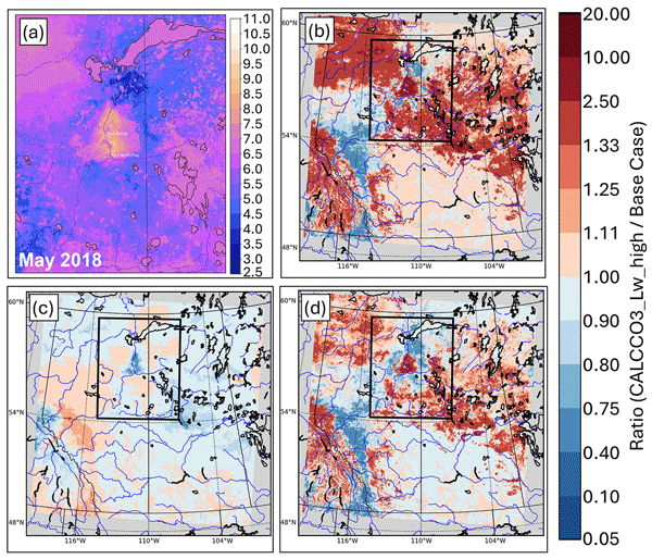
The AOSR appears as a distinct region of relatively alkaline foliage (7.5 ≤ pH ≤ 9.0), Figs. 6–8, panels (a). Downwind of the AOSR, the foliage pH decreases – first becoming neutral, then progressively more acidic (pH < 5.5) in May (Fig. 6a), with pH's of 6.5 to 7.5 downwind of the Oil Sands facilities in June (Fig. 7a) and July (Fig. 8a). The highest pH levels (>9, orange to yellow colours in panel (a) of Figs. 6–8) are located close to the open pit mine facilities for all three months – that is, close to the source of base-cations originating in fugitive dust. This spatial trend is consistent with the known behaviour of atmospheric PM in the region. The alkaline leaf surfaces in the AOSR are primarily due to coarse mode dust, which contains high levels of base cations and is deposited relatively close to emission sources (Zhang et al., 2018a). In contrast, particulate sulphate is predominately found in the fine mode and can be transported much further downwind, beyond the zone of significant alkaline dust deposition. As a result, acidic conditions dominate further from the source region, where the neutralizing influence of base cations diminishes. This pattern is also consistent with findings from Makar et al. (2018) who showed that at downwind distances less than 140 km from Oil Sands sources base cations are likely in excess relative to anions. Further insight is provided by examining the predicted composition of particulate matter deposited onto foliage in areas where high foliage pH values are predicted (e.g. central high pH region, Figs. 6–8, panels a). These regions receive a large fraction of deposited mass as particulate calcium, mainly in the form of calcium carbonate (CaCO₃) (Watson et al., 2014; Wang et al., 2015). Upon deposition and dissolution in the leaf water layer, CaCO₃ hydrolyses, raising the pH, consistent with the alkaline areas predicted in Figs. 6–8, panels (a). This results in substantial increases in the SO₂ deposition velocity (brown regions, Figs. 6–8, panels b), decreases in the SO₂ surface concentration (blue regions, Figs. 6–8, panels c), and increases in the SO₂ dry deposition flux (brown regions, Figs. 6–8, panels d).

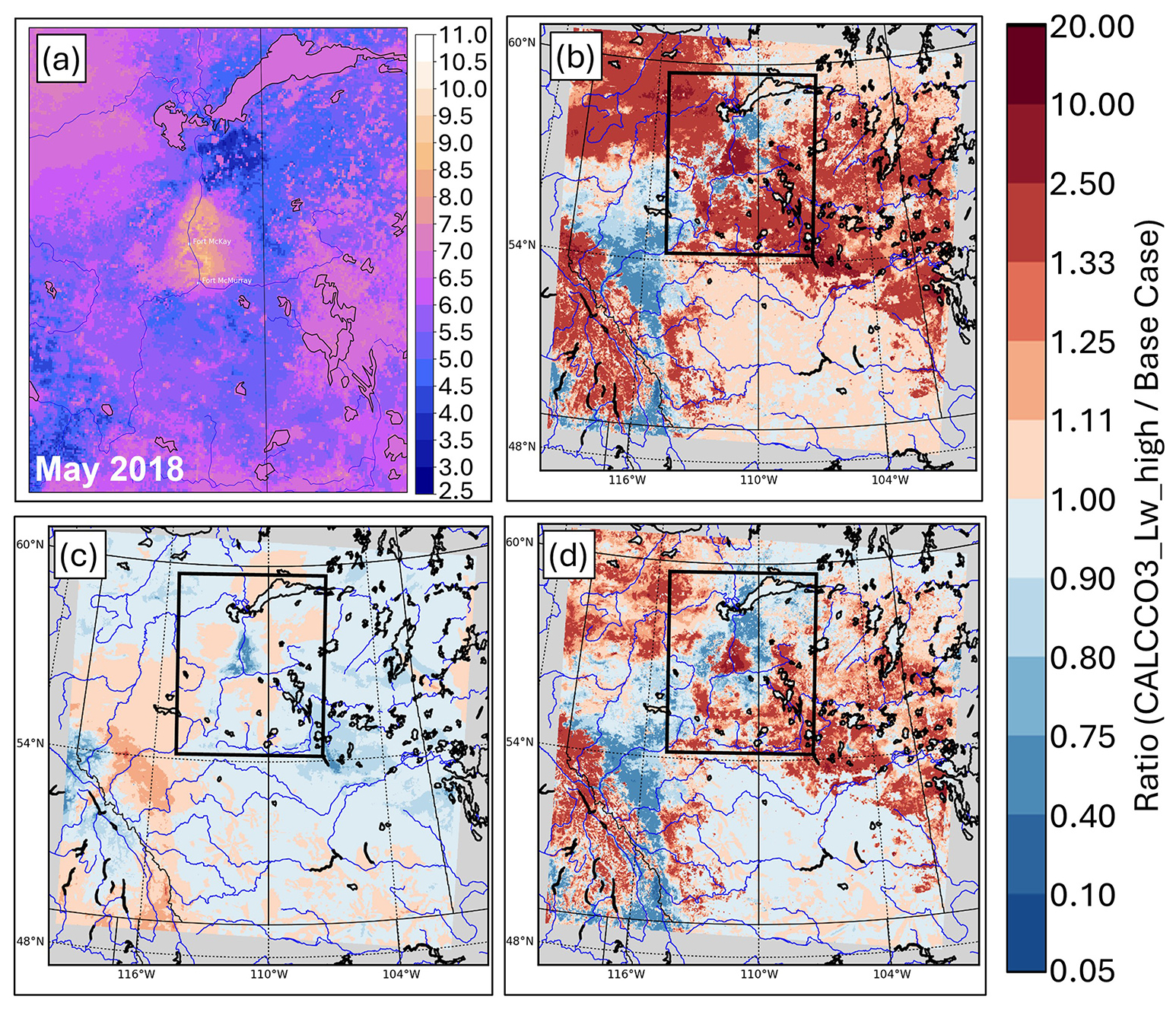
Figure 6 Average impact of surface foliage pH. May, 2018. (a) AOSR average surface foliage pH calculated using CALCCO3_Lw_high. (b, c, d) Ratios (CALCCO3_Lw_high : Base Case) of (b). $V_{{\mathrm{d}}_{{\mathrm{SO}}_{\mathrm{2}}}}$, (c) SO₂ concentration at the surface, (d) Monthly SO₂ deposition flux at the surface. Inset box in (b), (c), (d) shows the AOSR, displayed as a “zoom” in (a). Figure S3 shows the Base Case and CALCCO3_Lw_ high values corresponding to (b), (c), (d).

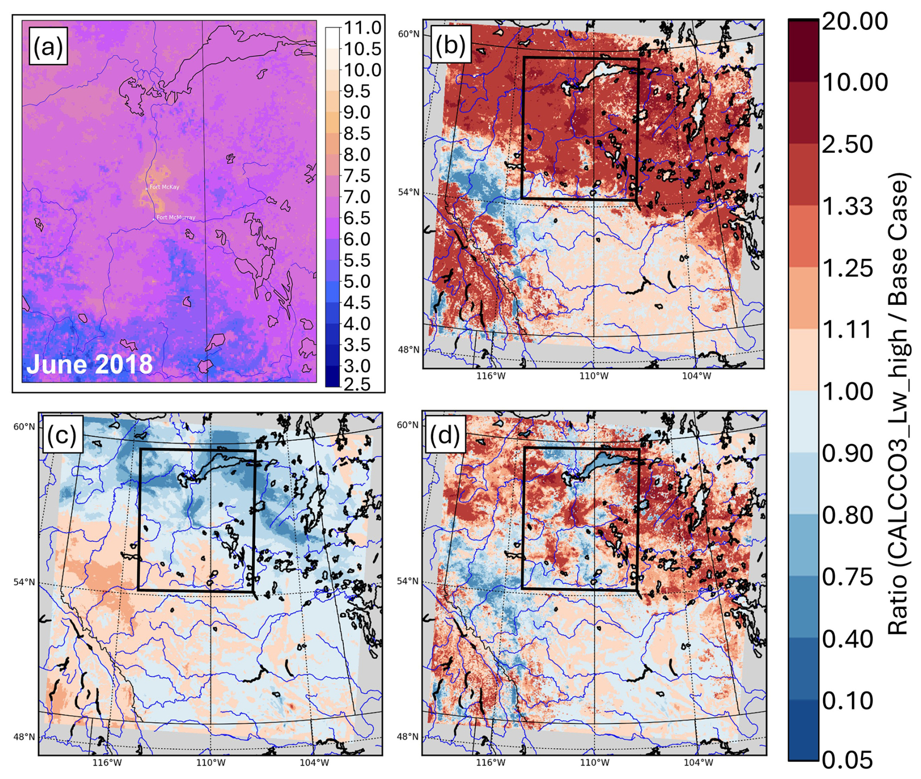
Figure 7 Average impact of surface foliage pH. June, 2018. Panels as in Fig. 6. Figure S4 shows the Base Case and CALCCO3_Lw_high values corresponding to (b), (c), (d).

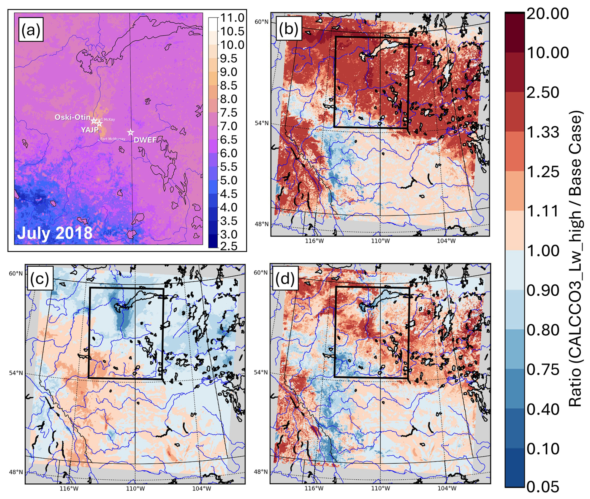
Figure 8 Average impact of surface foliage pH. July, 2018. Panels as in Fig. 6. Figure S5 shows the Base Case and CALCCO3_Lw_high values corresponding to (b), (c), (d). The locations of Oski-otin, YAJP and DWEF (stars) are provided for reference to Fig. 9.

Outside of the region influenced by Oil Sands facility fugitive dust, background pH levels increase from May and June (compare Fig. 6a with Figs. 7a, 8a) due to additional base cation deposition originating in forest fire particulate matter emissions, which increase towards the summer.

All three months show a substantial increase in $V_{{\mathrm{d}}_{{\mathrm{SO}}_{\mathrm{2}}}}$ relative to the base case (Figs. 6–9, panels b) with the use of the CALCCO3_Lw_high pH-dependent deposition algorithm in regions influenced by substantial base cation deposition. Base case deposition velocities over the domain range from 0.4 to 1.0 cm s⁻¹, while reaching 4.0 cm s⁻¹ for CALCCO3_Lw_high (see Figs. S3, S4, S5), with monthly average (CALCCO3_Lw_high) : (Base Case) ratios between 1.33 and 2.5 becoming common in the latter months in the boreal forest area. Ratios between 2.5 and 10 are present in the Oil Sands area in all three months due to the emissions of open pit mine fugitive dust from those facilities. Ratios of $V_{{\mathrm{d}}_{{\mathrm{SO}}_{\mathrm{2}}}}$ also reach values greater than 2.5 in areas of forest fire emissions in all three months (e.g. top left corner Fig. 8b). The ratios of $V_{{\mathrm{d}}_{{\mathrm{SO}}_{\mathrm{2}}}}$ in the AOSR are consistent with aircraft measurements from Hayden et al. (2021), who observed that measured (inferred) $V_{{\mathrm{d}}_{{\mathrm{SO}}_{\mathrm{2}}}}$ was 1.7 to 5.4 times larger than Base Case predictions from GEM-MACH simulations lacking the pH correction described here.

Investigation of wildfire ash chemical composition support the importance of forest fire emissions towards foliage pH, with studies showing that CaCO₃ is a major component; its dissolution in water often resulting in alkaline solutions with pH > 7.5, and sometimes as high as 11 (Sánchez-García et al., 2023; Pereira et al., 2013, 2012). Conversely, in the Foothills of Alberta where the foliage pH is often predicted to be acidic (blue regions Figs. 6–8, panels b), CALCCO3_Lw_high predicts a 20 % to 25 % reduction in $V_{{\mathrm{d}}_{{\mathrm{SO}}_{\mathrm{2}}}}$, highlighting that the pH-modulated $V_{{\mathrm{d}}_{{\mathrm{SO}}_{\mathrm{2}}}}$ can vary substantially across the domain, depending on the chemical composition of the mass deposited onto foliage.

As the pH increases above 9.0, both $r_{{\mathrm{cut}}_{\mathrm{zha}}}\left({\mathrm{SO}}_{\mathrm{2}}\right)$ and the canopy resistance r_c(SO₂) approach zero (see Fig. 2). In this work, a minimum value of 10⁻² s m⁻¹ was imposed on r_cut, which is much lower than the 20 s m⁻¹ limit suggested by Zhang et al. (2003) under wet conditions. Applying the 20 s m⁻¹ threshold would dampen the pH effects on $V_{{\mathrm{d}}_{{\mathrm{SO}}_{\mathrm{2}}}}$ beyond a pH of 8.0. However, the Zhang et al. (2003) threshold was not based on field measurements. While Sorteberg and Hov (1996) noted that no such measurements existed, more recent studies have reported r_c(SO₂)≈0, particularly in wet conditions (Neirynck et al., 2011; Feliciano et al., 2001). These findings suggest that r_cut(SO₂)≪20 s m⁻¹ is plausible. If very low $r_{{\mathrm{cut}}_{\mathrm{zha}}}\left({\mathrm{SO}}_{\mathrm{2}}\right)$ lead to unrealistic V_d estimates, this may reflect issues with the parameterization of r_a and r_b, rather than with $r_{{\mathrm{cut}}_{\mathrm{zha}}}$ itself.

Figures 6–8 (panels c) show the response of surface SO₂ concentrations towards these changes in $V_{{\mathrm{d}}_{{\mathrm{SO}}_{\mathrm{2}}}}$. The largest decreases occur in the AOSR (ratios between 0.40 and 0.75; reductions of 0.25 to 0.75 ppb, see also Figs. S3, S4, S5). Large ratio decreases in SO₂ of between 0.40 and 0.75 can also be seen throughout the northern part of the domain in June (Fig. 7c), a particularly active forest fire base cation emissions and deposition month in 2018. However, in these areas the absolute change is small (<0.1 ppb, see Fig. S4), limiting practical significance despite the large percentage difference. Localized SO₂ concentration increases of 10 % to 30 % are predicted in some regions, including the Foothills of Alberta and west of Cold Lake (orange colours, Figs. 6–8, panels c), where corresponding decreases in $V_{{\mathrm{d}}_{{\mathrm{SO}}_{\mathrm{2}}}}$ have been predicted (panels b). Although the absolute increases are typically <0.1 ppb (Figs. S3, S4, S5), there are localized areas exceeding 0.25 ppb. In absolute terms this decrease in the mean $V_{{\mathrm{d}}_{{\mathrm{SO}}_{\mathrm{2}}}}$ is much less than the increase seen in the AOSR, which often exceeds 1.0 cm s⁻¹. This result demonstrates that even a relatively small decrease in the mean $V_{{\mathrm{d}}_{{\mathrm{SO}}_{\mathrm{2}}}}$ (due to acidic foliage conditions) may cause a disproportionately large (localized) increase in the simulated mean surface SO₂ concentration. We note that the largest concentration decreases (blue colours, Figs. 6–8, panels c) correspond to areas and times where there is a high local deposition flux of base cations, from the Oil Sands facilities' fugitive dust emissions, or from forest fires.

The net impact of the changes on the SO₂ deposition flux (DSO2) is shown in Figs. 6–8 (panels d). As outlined in Sect. 4, DSO2 is the flux calculated on a time-step basis as the product of $V_{{\mathrm{d}}_{{\mathrm{SO}}_{\mathrm{2}}}}$ and the surface SO₂ concentration. Thus, increases in $V_{{\mathrm{d}}_{{\mathrm{SO}}_{\mathrm{2}}}}$ only translate to increased DSO2 where appreciable surface SO₂ concentrations are present. Where SO₂ is available, however, higher $V_{{\mathrm{d}}_{{\mathrm{SO}}_{\mathrm{2}}}}$ will proportionally increase DSO2, all else being equal. Accordingly, the largest absolute increases in DSO2 under CALCCO3_Lw_high occur in the AOSR, where elevated $V_{{\mathrm{d}}_{{\mathrm{SO}}_{\mathrm{2}}}}$ (2.5–10 cm s⁻¹) coincide with elevated surface SO₂ concentrations (>2 ppb). Since SO₂ emissions are identical in both Base Case and CALCCO3_Lw_high simulations, this increased flux is entirely attributable to changes in $V_{{\mathrm{d}}_{{\mathrm{SO}}_{\mathrm{2}}}}$ resulting from base cation-driven co-deposition. This enhancement is consistent with aircraft-based measurements reported by Hayden et al. (2021), who found that an earlier version of GEM-MACH, lacking the pH $V_{{\mathrm{d}}_{{\mathrm{SO}}_{\mathrm{2}}}}$ enhancement, underpredicted the dry deposition flux of total oxidized sulphur (TOS) by 2 to 14 times. While TOS measured in their study also included particulate sulphate, over 92 % of TOS their campaign was in the form of gaseous SO₂ making it reasonably representative of $V_{{\mathrm{d}}_{{\mathrm{SO}}_{\mathrm{2}}}}$.

Further downwind, particularly beyond 100 km from the AOSR, DSO2 is reduced relative to the Base Case by up to 40 %, especially in May (Fig. 6). Two factors contribute to this reduction – (1) depletion of SO₂ from upwind deposition and (2) local inhibition of deposition to acidic foliage conditions. The latter likely dominates, based on the spatial patterns: in regions where DSO2 is reduced under CALCCO3_Lw_high, surface SO₂ concentrations are increased relative to the Base Case, particularly in May (Fig. 6) – this occurs despite enhanced SO₂ removal to forests just upwind.

5.3 Comparison of modelled $V_{{\mathrm{d}}_{{\mathrm{SO}}_{\mathrm{2}}}}$ and SO₂ at surface monitoring network observations

Three locations in the 2.5 km model domain; Oski-otin (near the village of Fort Mackay), the York Athabasca JackPine site (YAJP), and a downwind evergreen forest location near the Saskatchewan border (DWEF) are superimposed on the monthly average leaf pH field in Fig. 8a, and their corresponding diurnal cycles of $V_{{\mathrm{d}}_{{\mathrm{SO}}_{\mathrm{2}}}}$ for the months of May and June are shown in Fig. 9. The DWEF site was selected to represent a downwind location where anthropogenic dust deposition is minimal and foliage water layers are often acidic to near neutral. This contrasts with both YAJP and Oski-otin, where deposition of alkaline dust frequently raises the foliage pH above 7.5 (see Figs. 6–8, panels a). As expected from Figs. 6–8 (panels a), YAJP and Oski-otin show substantial increases in $V_{{\mathrm{d}}_{{\mathrm{SO}}_{\mathrm{2}}}}$ when CALCCO3_Lw_high is applied. At these sites, the mean $V_{{\mathrm{d}}_{{\mathrm{SO}}_{\mathrm{2}}}}$ exceeds 1.0 cm s⁻¹ at all hours of the day, except in May at Oski-otin. Although the average remains high, individual values of $V_{{\mathrm{d}}_{{\mathrm{SO}}_{\mathrm{2}}}}$ vary widely – from as low as 0.5 cm s⁻¹ to over 4.0 cm s⁻¹ – as reflected in the large interquartile range (IQR). In the afternoon, the IQR exceeds 2 cm s⁻¹ at YAJP and Oski-otin indicating strong temporal variability. In contrast, the Base Case rarely predicts a $V_{{\mathrm{d}}_{{\mathrm{SO}}_{\mathrm{2}}}}$ that exceeds 0.5 cm s⁻¹ at these locations, with a much narrower IQR around 0.2 cm s⁻¹. A notable exception occurs at Oski-otin in May between 12:00 to 00:00, where the median, 25th and 75th percentile for CALCCO3_Lw_high closely match those of the Base Case. This is due to insufficient predicted foliage water, leading to the pH being reset to 6.68 (the same constant value used in the Base Case). Nonetheless, the mean $V_{{\mathrm{d}}_{{\mathrm{SO}}_{\mathrm{2}}}}$ during this period is still much higher than median, implying that a small number of very high values significantly raises the mean.

The $V_{{\mathrm{d}}_{{\mathrm{SO}}_{\mathrm{2}}}}$ predicted by CALCCO3_Lw_high at Oski-Otin and YAJP are in the range of $V_{{\mathrm{d}}_{{\mathrm{SO}}_{\mathrm{2}}}}$ inferred from tower and aircraft measurements reported in Hayden et al. (2021) and Gordon et al. (2023). Specifically, Hayden et al. (2021) measured $V_{{\mathrm{d}}_{{\mathrm{SO}}_{\mathrm{2}}}}$ at a tower site in the AOSR over a three-day period (6 to 8 June 2018), finding a mean afternoon value (13:00 to 19:00 Mountain Daylight Time) of 4.1 cm s⁻¹, with minimal uptake of SO₂ during the night ($V_{{\mathrm{d}}_{{\mathrm{SO}}_{\mathrm{2}}}}$ < 0.5 cm s⁻¹). These values fall well within the diurnal ranges predicted by CALCCO3_Lw_high at Oski-otin (see Fig. 9). Aircraft-based estimates from Hayden et al. (2021) (conducted between 13 August and 7 September 2013) reported afternoon $V_{{\mathrm{d}}_{{\mathrm{SO}}_{\mathrm{2}}}}$ values ranging from 1.2 to 3.4 cm s⁻¹. Although these measurements were made in a different year and spanned various surface types (i.e., forests, lakes, wetlands and tailings ponds) they also align well with the CALCCO3_Lw_high predictions. At YAJP, Gordon et al. (2023) inferred $V_{{\mathrm{d}}_{{\mathrm{SO}}_{\mathrm{2}}}}$ between July and October 2021, reporting values between 2.1 and 5.9 cm s⁻¹. While the Gordon et al. (2023) measurement period does not overlap with the 2018 model simulations shown in Fig. 9, similar magnitudes of anthropogenic dust deposition in both years suggest comparable pH conditions, and consequently, similar SO₂ uptake rates. In summary, all three observational datasets report $V_{{\mathrm{d}}_{{\mathrm{SO}}_{\mathrm{2}}}}$ values within the range predicted by CALCCO3_Lw_high, reinforcing that the pH-dependent deposition algorithm offers a substantial improvement over the Base Case in replicating observed $V_{{\mathrm{d}}_{{\mathrm{SO}}_{\mathrm{2}}}}$ in the AOSR.

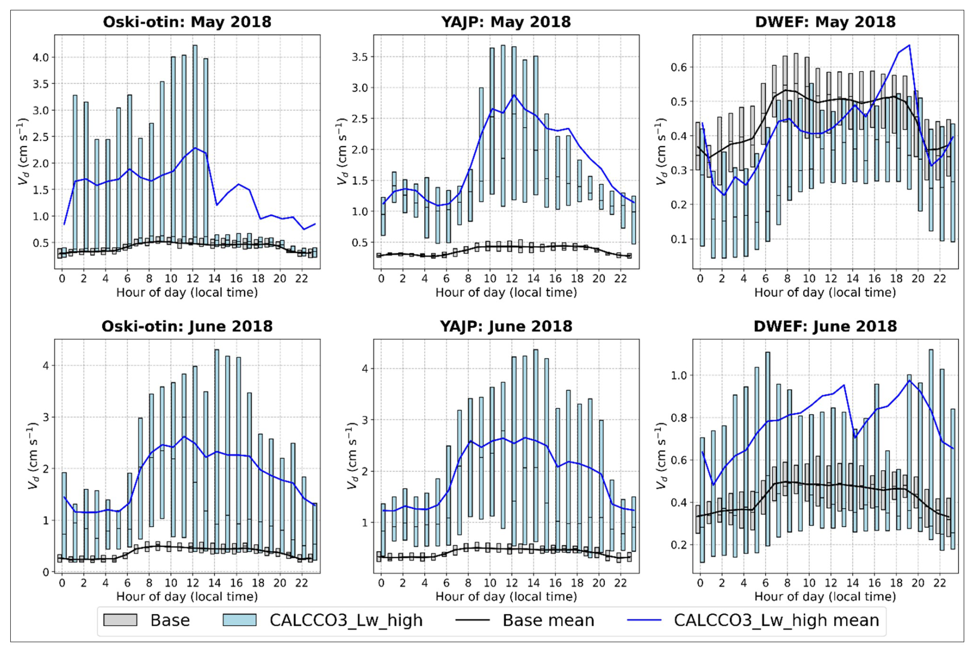
Figure 9 The diurnal cycle of model-predicted $V_{{\mathrm{d}}_{{\mathrm{SO}}_{\mathrm{2}}}}$ at (a, d) Oski-otin, (b, e) the York Athabasca Jack Pine (YAJP) Tower, (c, f) a downwind evergreen forest (DWEF). The first row (a, b, c) shows the predicted $V_{{\mathrm{d}}_{{\mathrm{SO}}_{\mathrm{2}}}}$ for May 2018 while the second row (d, e, f) shows June 2018. The box plot formatting in Fig. 9 is consistent with Fig. 5 and solid lines indicate the mean $V_{{\mathrm{d}}_{{\mathrm{SO}}_{\mathrm{2}}}}$ in each hourly bin.

Time series of both observed and simulated mean diurnal cycles of the surface SO₂ concentration at 20 different WBEA continuous monitoring stations (Figs. 10, S7, S8, S9, and 11, S10) show that the pH-modulation effect has the most pronounced impact on the mean surface SO₂ concentrations (relative to the Base Case) at the stations BGFM, FMCS, HRZN, MUSK, FTHL and WAPI, though improvements in NMB can be seen in 13 and 15 out of 21 stations in June and August 2018 respectively (Fig. 11a, b). At the six stations with larger improvements, CALCCO3_Lw_high yields a substantial reduction in the normalized mean bias (NMB) relative to the Base Case (Table 1, see also Fig. 11a, b).

Table 1 Example NMB score changes by station, June 2018 (see also Fig. 11b).

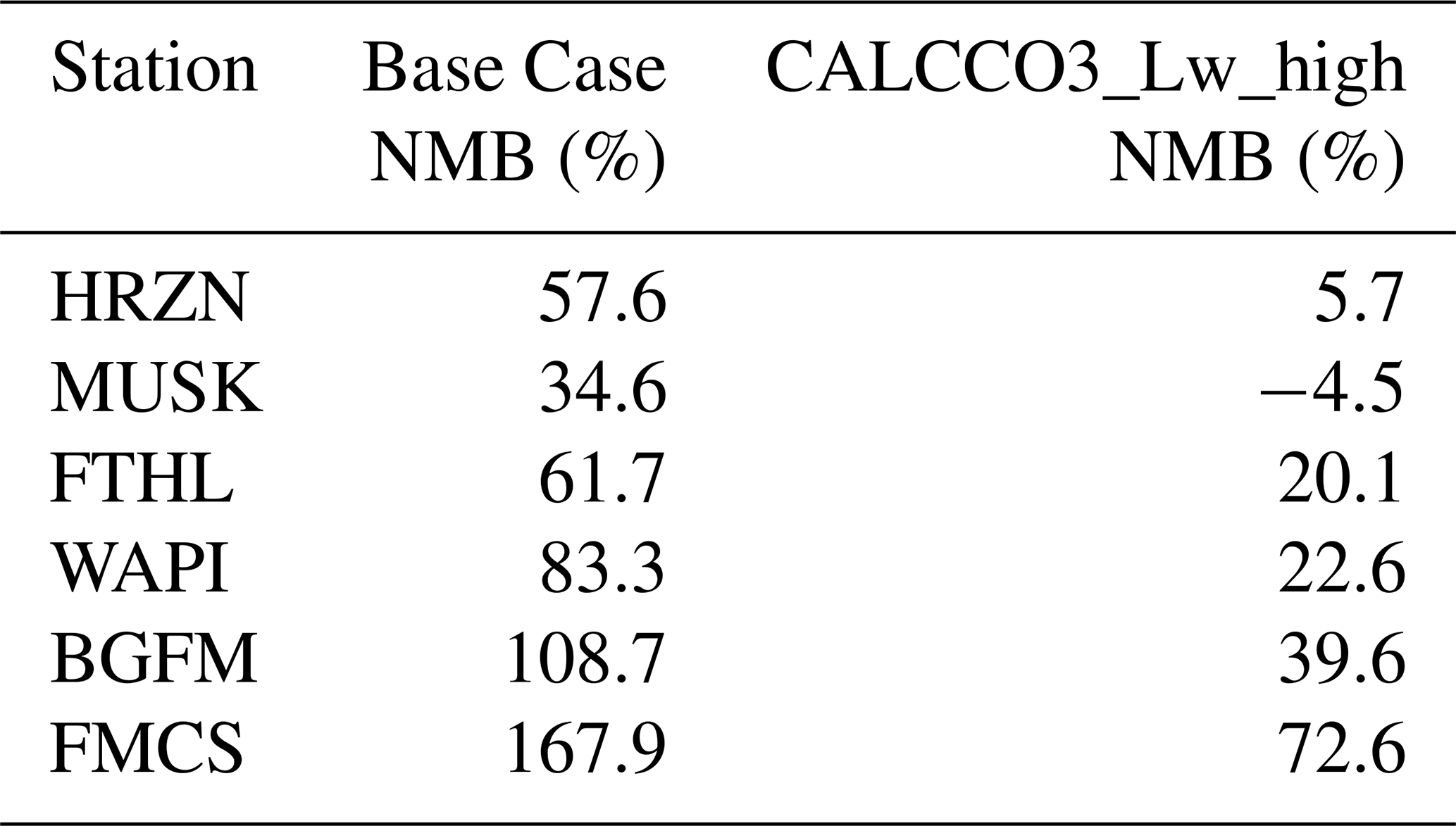
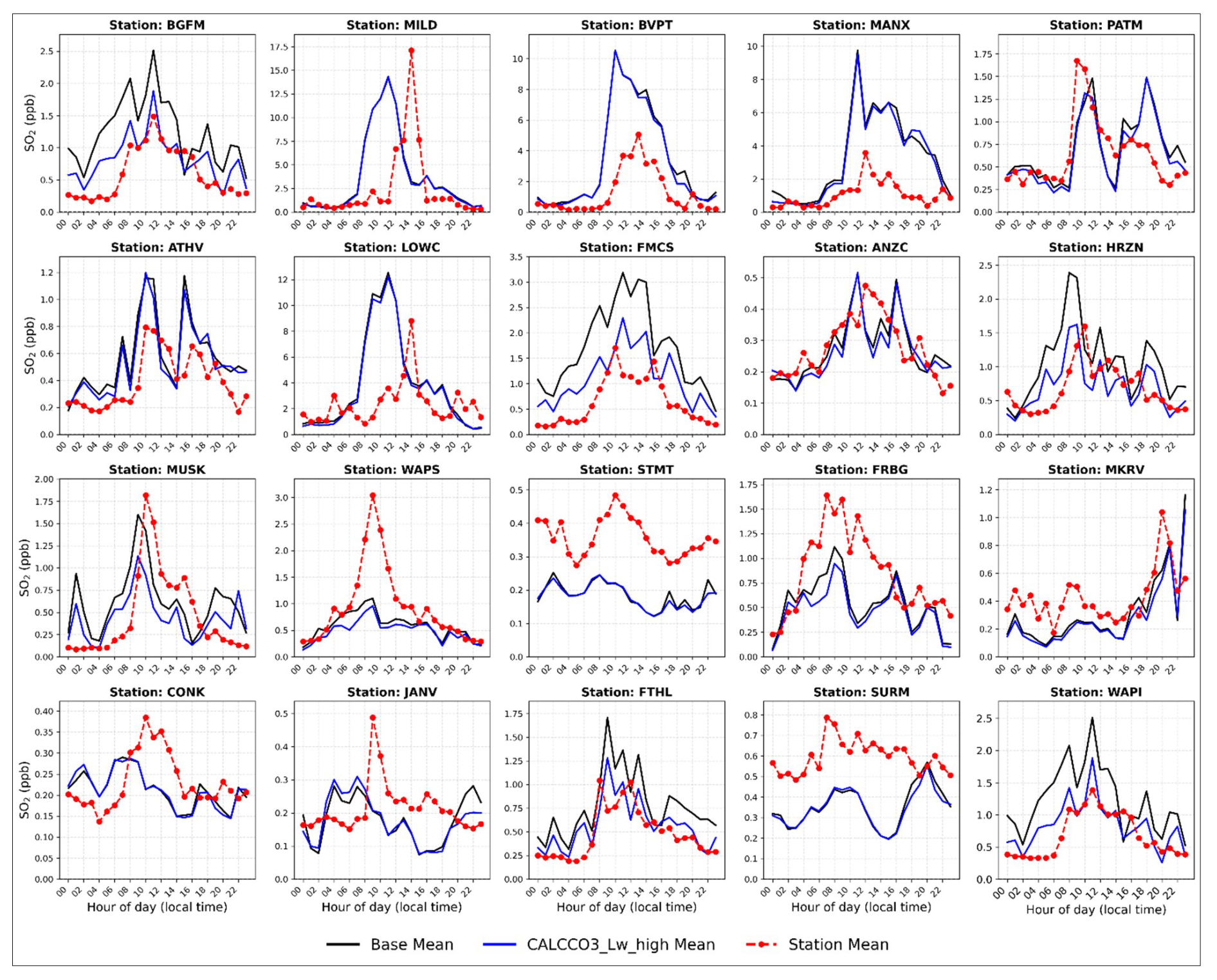
Figure 10 The mean diurnal cycle of SO₂ measured at WBEA continuous monitoring stations (red dashed line) given in local time. The data are for the month of June 2018. Also shown are the model predicted mean SO₂ surface concentrations at the same location. The black line is the Base Case, while the blue line is CALCCO3_Lw_high. Note that due to plotting limitations the WBEA station “FTCH” is not included in the figure. Identical plots for May, July and August 2018 are provided in the Supplement (Figs. S5, S6, S7, respectively).

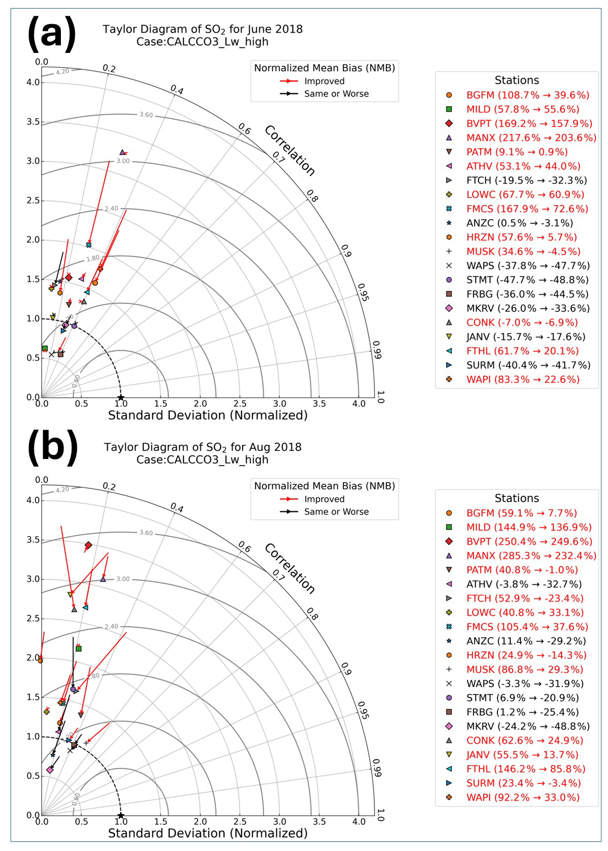
Figure 11 Taylor Diagram of SO₂ for (a) June 2018, (b) August 2018 (see Fig. S10 for May and July). The equations used to compute these metrics are provided in Table S3. In each panel, the “star” symbol on x-axis marks the reference point for a perfect model, corresponding to a correlation = 1.0, a CRMS = 1.0 and a normalized standard deviation = 1.0. Arrows illustrate changes in model performance from the Base Case (arrow start) to CALCCO3_Lw_high (arrow end). A trajectory that moves closer to the reference point indicates improved agreement with observations (red arrows). The CRMS is proportional to the distance from the star; concentric circles centred on the star represent contours of constant CRMS. The standard deviation is measured radially from the origin. The different WBEA stations are denoted by different symbols, with each arrow pointing from the Base Case to CALCCO3_Lw_high locations of station performance on the diagram. Red (black) arrows denote an improvement (deterioration or no change) in the normalized mean bias error (NMB) for CALCCO3_Lw_high compared to the Base Case. The value of the NMB for each station is shown in the legend after the station name as (Base Case → CALCCO3_Lw_ high), with red text likewise representing improvements in the NMB when using CALCCO3_Lw_high compared to the Base Case. The azimuthal distance represents the correlation (i.e., r) starting from 0.0 and increasing clockwise to 1.0. The radial distance from the origin gives the normalized standard deviation of the model at the station. Each station standard deviation has been normalized by the observed standard deviation at that station. Thus, the observed standard deviation is always at (1.0, 1.0) represented by the star on each plot. May and July Taylor diagrams are given in the Supplement, Fig. S10.

Notably, WAPI is the same tower site where Hayden et al. (2021) inferred $V_{{\mathrm{d}}_{{\mathrm{SO}}_{\mathrm{2}}}}$ during a 3 d period in June 2018. During May 2018, these same stations often show an improvement in the NMB during the afternoon when CALCCO3_Lw_high is applied. However, at night CALCCO3_Lw_high tends to underpredict surface SO₂ concentrations more severely than the Base Case. This systematic underprediction, also present to a lesser extent in the Base Case (typically by ∼ 0.5 ppb), suggests a broader issue likely related to the quasi-laminar sublayer resistance (r_b). Specifically, it may indicate that the nocturnal atmospheric stability is not properly represented in the model; r_b may not be sufficiently enhanced in response to suppressed turbulence, leading to an overestimation of SO₂ deposition. This may also suggest that the GEM model underrepresents nocturnal atmospheric stability, possibly due to excessive turbulent mixing or an inadequate parameterization of resistances in stable boundary layers. A similar nighttime underprediction pattern appears in July. In August, however, CALCCO3_Lw_high does a better job simulating the nighttime SO₂ surface concentrations than the Base Case. The Base Case often overpredicts the mean surface SO₂ concentration during the nighttime, while CALCCO3_Lw_high shows much better agreement overall, with a NMB at most stations that is closer to 0 % (i.e., Fig. 11a, b).

Figure 11 presents Taylor diagrams for (panel a) July and (panel b) August 2018 (see Fig. S10 for May and June); these summarize graphically how closely modelled surface SO₂ concentrations match observations (Taylor, 2001). The diagrams simultaneously depict three key statistics: the correlation coefficient, the centred root-mean square difference (CRMS), and the standard deviation (amplitude of variation). In this work, both model and observed values are normalized by the observed standard deviation, giving a normalized standard deviation. This implies that the observations always have a standard deviation of 1.0, marked as a black dashed line (semicircle) at a radius of 1.0 on each plot. Arrows that move closer to this dashed line indicate improved agreement in the amplitude of variation. The azimuthal angle represents the correlation, increasing clockwise from 0.0 to 1.0. To aid interpretation, the normalized mean bias (NMB) for each station is listed in the legend as (Base Case → CALCCO3). Red text and red arrows highlight stations where CALCCO3_Lw_high produces a better NMB than the Base Case. Black arrows indicate no improvement or a deterioration in the NMB. A general result of the comparison is that NMB values “shift towards negative numbers” – that is, all NMB values are decreasing. For stations where the base case NMB was positive this usually results in a smaller magnitude positive or negative NMB (red tabulated numbers), and for stations where the base case NMB was negative, the NMB becomes more negative (black tabulated numbers). Additional factors aside from the pH effect studied here are therefore likely to result in the remaining station-to-station variations in NMB. The results show that CALCCO3_Lw_high improves the standard deviation at several stations compared to the Base Case, especially in June (e.g., at BGFM, HRZN, FMCS, FTCH, FTHL, LOWC) and even more so in August, where all stations except BVPT, ANZC, MKRV and WAPS show improvement. In contrast, July exhibits mostly a deterioration in the standard deviation (see Fig. S10), with many arrows pointing away from the reference line at 1.0, indicating poorer agreement with observed variability.

Despite modest to large statistical improvements in NMB in May, June, July and August at some stations, substantial discrepancies remain between modelled and observed surface SO₂ concentrations, particularly in the form of low correlation coefficients (i.e., correlation ≪ 1.0). While dry deposition plays a key role in determining the surface SO₂ concentrations in GEM-MACH, other factors may also contribute significantly to correlation, including:

• i.

  the accuracy of meteorological variables predicted by GEM (i.e., air temperature, wind speed and direction, boundary-layer stability, precipitation occurrence and timing),

• ii.

  the accuracy of SO₂ point-source emissions, including stack parameters required for plume rise calculations, as well as the fidelity of the plume rise algorithm itself (Fathi et al., 2025),

• iii.

  chemical transformation of SO₂, particularly the aqueous-phase oxidation to sulphate in cloud droplets or within emission plumes, along with the cloud to rain conversion process governing wet deposition, and

• iv.

  the effect of model grid resolution (Russell et al., 2019) which dilutes point-source emissions over much broader areas, smoothing out localized gradients.

In addition to the factors listed above, instrumental limitations in the observations must also be considered. WBEA monitors employ continuous SO₂ analysers that are subject to a trace detection limit of 0.2 ppbv (AEP, 2014), below which concentrations are reported as zero. In contrast, GEM-MACH has no lower bound on predicted SO₂ concentrations, meaning it can simulate values that fall below the detection threshold and would therefore be recorded as below threshold in observations. Taken together, these points suggest that pH-modulated dry deposition alone cannot fully reconcile the modelled and observed SO₂ concentrations. However, as demonstrated in Fig. 11, the implementation of CALCCO3_Lw_ high yields improvements in the NMB, and trajectories indicating improvements for correlation coefficient, CRMS, and standard deviation, for many stations.

6 Uncertainties and Observation Needs

While we have identified the potential for base cation co-deposition to significantly influence SO₂ deposition velocities and fluxes, there are several potential sources of uncertainty in this work, meriting further research. Many of these would require the collection of new observation data in order to be resolved. Several assumptions or omissions in our model reflect these potential uncertainties in the prediction of foliage pH and its effect on the SO₂ dry deposition velocity. Key limitations include:

1. Bulk canopy treatment: The foliage pH is modelled as a single value per grid cell, despite field observations showing strong vertical variability within a single forest stand (Fritsche, 1992)

2. Simplified particle deposition: The particle collection efficiency ${\mathit{\eta }}_{{\mathrm{veg}}_{\mathrm{sp}}}$ depends only on the LAI and particle size, omitting effects of species-specific leaf morphology such as hairs, roughness and waves (Pryor et al., 2013; Grönholm et al., 2009; Donat and Ruck, 1999).

3. Leaf-surface microclimate simplification: The near-leaf relative humidity is likely elevated due to transpiration and boundary-layer effects (Boulard et al., 2002), but the model uses the ambient relative humidity to drive pH calculations. This may underestimate the water liquid water content on foliage where hygroscopic aerosols are present, affecting the ionic strength, and hence predicted pH of the leaf water layer on foliage (Tredenick et al., 2022; Coopman et al., 2021; Katata and Held, 2021; Burkhardt et al., 1999; Eiden et al., 1994).

4. Water and particle retention on foliage: The model does not account for the foliage water holding capacity (Wohlfahrt et al., 2006; Bradley et al., 2003; Brewer and Smith, 1997; Sellers et al., 1986) or the PM retention capacity (Zheng and Li, 2019; Chen et al., 2017) of the foliage. Neglecting the leaf water holding capacity may result in “false” washoff events during light precipitation where the leaf water holding capacity is not exceeded (i.e., no actual washoff occurs).

5. Wet deposition simplification: Wet deposition was excluded from foliage pH calculations, assuming that during precipitation only the removal of soluble dry deposition mass from foliage occurs. Given sufficient precipitation, complete washoff is assumed, resetting accumulators to near-zero and yielding near-neutral pH. However, this likely overestimates pH during and immediately after the precipitation event, as most precipitation has pH < 6 (Vet et al., 2014 and references therein). Wet deposition retention on leaves is poorly constrained due to limited data on how much precipitation mass is retained by foliage. Observational data from Fort McMurray (AOSR) indicate that measurable precipitation was rare (≤ 0.07 % of the time between May–August 2018), supporting the assumption that dry deposition dominates pH modulation in this region. Nonetheless, the simplification may not hold in wetter environments or during/after rain events, when wet deposition can transiently alter leaf surface chemistry.

6. Unmodelled surface chemistry: Processes such as SO₂ oxidation in the water layer boundary via soluble oxidants such as H₂O₂ (Chameides, 1987), organic acid buffering (Shigihara et al., 2008; Rogge et al., 1993; Tukey, 1966), foliar leaching (Tukey, 1966; Adams and Hutchinson, 1984; Adams and Hutchinson, 1987; Potter, 1991; Scherbatskoy and Tyree, 1990; Kohno et al., 2001) and bi-directional exchange (Wang et al., 2020; Massad et al., 2010; Flechard et al., 1999) are neglected.

7. Non-precipitation water sources: Fog, dew, and leaf guttation contribute to foliar moisture (Sects. 1.6 and 4.5). Dew adds only water, whereas guttation and fog can also deposit particle mass. Potential washoff due to dripping from these sources is neglected, and mass deposition from fog and guttation is ignored. Observational data show fog was rare (<0.02 % of the May to August 2018 period in the AOSR), supporting the assumption that these additional sources of wet removal are minimal in this region.

8. No particle resuspension: Particle resuspension from foliage due to wind shear is highly variable and depends on wind conditions, canopy structure, and leaf morphology (see Sect. 1). Due to these uncertainties and the likelihood that resuspended particles remain within the same model grid cell, wind-driven resuspension was not explicitly included in this study's deposition algorithm.

9. Resistance parameter uncertainty: the boundary layer resistance r_b and the aerodynamic resistance r_a are fixed based on literature parametrizations. Inaccuracies in these terms could contribute to model-observation discrepancies in V_d even in the absence of a pH feedback effect (Hayden et al., 2021).

10. Other: other sources of uncertainty include chemical aging of foliage, model emission errors (e.g., wildfires), unmodeled surfaces such as bark, and the impact of insects and microbes.

Having identified several key uncertainties and limitations associated with this work, particularly surrounding the prediction of foliage pH, which directly modulates $V_{{\mathrm{d}}_{{\mathrm{SO}}_{\mathrm{2}}}}$, we note that the level of uncertainty in simulating foliage pH is high due to the many poorly constrained biological, chemical, and physical processes that influence it. To improve the parameterization described in Sect. 3, a comprehensive and targeted suite of in-situ observations is needed. These observations should span a range of vegetation types, canopy structures, and environmental conditions to be broadly representative. Some specific data needs include:

1. Measurements of the vertical variation of foliage pH within canopies. Since canopy-level pH is currently treated as a bulk value, vertical profiles of leaf-surface [H⁺] at different heights within the canopy are needed to determine whether a layered or height-dependent approach is more appropriate.

2. Measurements of particle collection efficiency ${\mathit{\alpha }}_{{\mathrm{cut}}_{{\mathrm{p}}_{\mathrm{sp}}}}$ across multiple plant forest types are needed to refine deposition estimates (currently the only factor considered is leaf area index).

3. Measurements of the chemical composition of leaf surface water layers. In-situ sampling of thin water films for ionic composition (including base cations, nitrate, sulfate, and organic acids/bases) would help validate the HETP and CALCCO3 chemical modules and constrain assumptions about neglected organic species.

4. Measurements of particle mass and chemical composition deposited on to foliage via fog and guttation are needed to assess whether this process is significant.

5. While lab-based estimates of leaf water holding capacity help determine the potential for retention, what is critically needed are field observations of actual washoff events across a range of plant species, canopy structures, and rainfall intensities. These should quantify both the timing and chemical composition of material removed from foliage during precipitation. Such data would help determine when light rainfall leads to retention versus wash-off of deposited material and would inform improvements to model algorithms that currently rely on oversimplified thresholds. Ideally, these measurements would capture (1) the onset of washoff relative to cumulative rainfall, (2) the fraction of dry-deposited mass removed, (3) variability by leaf type and canopy exposure, and (4) how the chemical composition of washoff differs from precipitation input.

6. Wind tunnel and in-situ field studies measuring resuspension rates across wind regimes, canopy densities, and species types would help quantify the extent to which resuspended mass remains in-canopy opposed to being deposited to the ground.

7. Finally, it is imperative that whenever dry deposition velocities of SO₂ are inferred from in-situ measurements (whether by flux towers or aircraft campaigns) a complementary characterization of the foliage is conducted. This includes not only direct quantification of leaf wetness (e.g., via electrical conductance) but also measurements of the pH of the thin aqueous layers on the foliage. Without such information, it is difficult to interpret SO₂ deposition estimates or validate model predictions with confidence.

7 Conclusions

Despite the above uncertainties, this work has shown that the deposition of base cations to the forests downwind of the AOSR can modify the pH of thin water layers present on the foliage, and that these modifications can have significant local impacts on SO₂ deposition velocities, concentrations and deposition fluxes. For example, forests immediately downwind of the AOSR often have foliage water layers with a pH exceeding 7.5, while further downwind forests have foliage that is more acidic (pH < 5.0) since the co-deposition of base cations and gaseous SO₂ no longer occurs in significant amounts. Incorporating a pH feedback effect into the dry deposition code (specifically by allowing the predicted foliage pH to modify the effective Henry's law constant for SO₂) results in an increase of $V_{{\mathrm{d}}_{{\mathrm{SO}}_{\mathrm{2}}}}$ in the AOSR by 2.5 to 10× (relative to a Base Case without any feedback effect). This increase brings modelled $V_{{\mathrm{d}}_{{\mathrm{SO}}_{\mathrm{2}}}}$ in the range of observations (ground-based and aircraft) made in the vicinity of the facilities, where the mean $V_{{\mathrm{d}}_{{\mathrm{SO}}_{\mathrm{2}}}}$ often exceeds 2 cm s⁻¹ during the afternoon.

The impact of modifying $V_{{\mathrm{d}}_{{\mathrm{SO}}_{\mathrm{2}}}}$ is also evident in the predicted mean monthly SO₂ surface concentrations and the monthly mean SO₂ dry deposition flux (Figs. 6–8, panels c, Figs. S3–S6); the former of which has decreased by up to 0.75 ppb (representing a decrease of up to 60 %) while the latter has increased by 2.5 to 10×. This decrease in the surface SO₂ concentrations represents an overall improvement to the model performance when the pH feedback effect is included, particularly in June and August. This improvement is represented in the statistical metrics calculated at the individual WBEA stations, especially at stations BGFM, FMCS, HRZN, MUSK, FTHL and WAPI, but can also be seen over large areas as a greater than factor of two change in deposition flux.

While these results have focused on a region with a combination of base cation emissions from anthropogenic fugitive dust and anthropogenic SO₂ emissions, we note that base cation deposition fluxes from natural sources may be very large, and are known to result in significant base cation deposition flux far downwind (in downwind continents from those with the emissions – Sahara and Asian dust events). Our results here suggest that forest fires are one such source of significant base cation emissions and deposition with large impacts on pH-modulated co-deposition of SO₂. We also note that a recent comparison of ensembles of regional air-quality models carrying out simulations for North American and European domains have shown that many models have positive biases of SO₂ in these regions, particularly at more remote sites, suggesting a need for a missing SO₂ loss mechanism (Makar et al., 2025), potentially filled here by base-cation co-deposition and SO₂ deposition enhancement due to pH effects.