Strong monsoon influence on South Asian methane emissions in 2020 revealed by a Bayesian inversion constrained by satellite observations

South Asia is a major contributor to global methane (CH₄) emissions, yet its emissions remain poorly constrained, limiting targeted mitigation. Current bottom-up inventories do not consistently capture the magnitude and seasonality of CH₄ emissions in this region, particularly during the monsoon. Here we quantify South Asian CH₄ emissions for 2020 using column observations from a satellite instrument (TROPOMI), a Lagrangian transport model (FLEXPART), and a Bayesian inversion system (FLEXINVERT+). We estimate a posteriori emission of 73.0 ± 0.7 Tg yr⁻¹ for South Asia, including 35.6 ± 0.5 Tg yr⁻¹ for India and 13.2 ± 0.4 Tg yr⁻¹ for Bangladesh. Agriculture and wetlands contribute substantially to the regional budget, with the flux increments coincident with rice-growing areas and inundated lowlands. The inversion indicates pronounced monsoon-modulated seasonality in South Asia: posterior fluxes are higher than the prior by about 19.3 Tg CH₄ (an increase of ∼ 70 %) during June–September and lower during January–May by ∼ 46 %. Localized enhancements seen over the lower Indus Basin align with runoff patterns, while the seasonal peaks here are absent in inventories. By resolving monsoon seasonality with satellite constraints, our results point towards key uncertainties in the South Asian CH₄ budget and underscore the need for process-based, seasonally responsive inventories to inform mitigation strategies and reconcile bottom-up and top-down estimates.

1 Introduction

Methane (CH₄) is a potent greenhouse gas with a global warming potential 84–87 times higher than that of carbon dioxide over a 20-year period (International Energy Agency, 2021). Understanding and accurately quantifying methane emissions is, therefore, crucial for developing effective climate mitigation strategies. South Asia (SA), with its diverse sources of methane emissions, including agriculture, waste, wetlands, energy production and use, presents a unique and complex domain for such studies. This region includes India, Pakistan, Bangladesh, Nepal, Bhutan and Sri Lanka. SA is one of the biggest methane emission hotspots in the world (Stavert et al., 2022), with its total emissions rising from 37 Tg yr⁻¹ in the 2000s to 75 Tg yr⁻¹ in the 2010s (Belikov et al., 2024). Patra et al. (2013) estimated 37 ± 3.7 Tg yr⁻¹ during the 2000s and Wang et al. (2021) estimated 64.35 ± 9.28 Tg yr⁻¹ emissions from the year 2009 to 2018 over South Asia. Among Asian countries, this region contributes to about 25.6 % of the total budget for Asia during 2001–2021 (Ito et al., 2023). As all of these are developing nations, their economic growth could cause a notable rise in anthropogenic emissions, particularly from agriculture.

India, the largest economy of the region, contributes more than half of these emissions, and is the key region of focus in this study. This region has been the focus of several country-scale studies. Ganesan et al. (2017) estimated average methane emissions of 22.0 (19.6–24.3) Tg yr⁻¹ during 2010–2015, while Raju et al. (2022) reported ∼ 10.63 Tg yr⁻¹ of methane emissions from Peninsular India (south of 21.5° N) for 2017–2018. More recent satellite-based studies give higher values, with Worden et al. (2022) estimating 39.5 ± (2.8–5.4) Tg yr⁻¹ of anthropogenic emissions for the year 2019 and Yu et al. (2023) reporting 36 (34–38) Tg yr⁻¹ of anthropogenic emissions for 2018–2019. India's National Communication reports its anthropogenic greenhouse gas emissions to UNFCCC in the form of Biennial Update Reports (BUR). These bottom-up reports estimate emissions of 19.8 (BUR-1), 20.05 (BUR-2), 19.55 (BUR-3) and 18.8 (BUR-4) Tg yr⁻¹, respectively, for the years 2010, 2014, 2016 and 2020 (Ministry of Environment, Forest and Climate Change, Government of India, 2016). The country's report also includes the top-down anthropogenic methane estimate of 24.2 ± 5.3 Tg yr⁻¹ for the years 2011-2017, taken from Janardanan et al. (2020). While there are not many studies over other regions of South Asia, Peters et al. (2017) report emissions for Bangladesh in the range of 1.3 to 3.1 Tg yr⁻¹ for the 2000s.

In a situation where bottom-up emission inventories are highly uncertain, top-down methods based on atmospheric measurements offer the possibility to verify or improve the bottom-up inventories. However, while regions like Europe and North America are covered with relatively dense ground-based GHG monitoring networks, only a few stations exist in South Asia. Moreover, access to high-quality data from the few existing sites is often limited or difficult, further hindering reliable budget estimates. In this context, satellite observations provide the essential alternative (Streets et al., 2013), capable of delivering spatially continuous and regionally representative methane measurements, making them indispensable for top-down emission estimation in regions such as South Asia.

The earliest satellite observations for methane were provided by the SCanning Imaging Absorption spectroMeter for Atmospheric CHartographY (SCIAMACHY) instrument onboard the European Space Agency's (ESA) ENVISAT satellite, launched in 2002 (Bovensmann et al., 1999). The launch of the first dedicated greenhouse gas monitoring satellite, GOSAT (Greenhouse Gases Observing Satellite) with its TANSO-FTS instrument developed by JAXA, in 2009 opened the possibility for monitoring carbon dioxide and methane emissions across the globe (Kuze et al., 2009). Since then, several other satellites have enhanced the GHG monitoring capabilities (Jacob et al., 2022). The TROPOspheric Monitoring Instrument (TROPOMI) on the ESA's Sentinel-5 Precursor satellite, launched in October 2017, provides high-resolution, daily global observations of atmospheric methane (Hu et al., 2016). The TROPOMI data offer unprecedented spatial and temporal coverage well suited for GHG estimation both on global and regional scales.

Satellite retrievals of methane are known to have systematic biases that vary by instrument, retrieval methodology and region, driven by factors such as surface albedo, aerosols, and clouds. Over Asia, these effects have been shown to translate into substantial differences in inferred emissions, with GOSAT and TROPOMI based inversions differing by up to 7.7 Tg yr⁻¹ over northern India and eastern China (Liang et al., 2023). Biases associated with surface reflectance, aerosol loading, and across-track striping in early TROPOMI products can exceed upto 10 ppb in some regions and have been linked to false methane anomalies caused by unmodelled surface spectral features or inadequate topographic information (Balasus et al., 2023; Jongaramrungruang et al., 2021; Lorente et al., 2023). Algorithm updates to the operational TROPOMI retrieval have substantially reduced albedo-dependent biases through improved spectroscopy, higher-resolution surface altitude data, and posteriori corrections (Lorente et al., 2021). The scientific TROPOMI WFMD product further addresses these issues by using higher-order polynomial fitting to better represent spectral albedo variability, updated digital elevation models, refined machine-learning based quality filtering, and orbit-wise destriping and calibration, resulting in reduced systematic errors and improved spatiotemporal consistency (Schneising et al., 2023). Notably, persistent seasonal biases present in the operational product at high latitudes are largely absent in WFMD (Lindqvist et al., 2024; Schneising et al., 2023).

Despite these advances, assimilating satellite column observations into inverse modeling systems remains challenging because column-averaged XCH₄ measurements have lower signal-to-noise ratio and weaker sensitivity to near-surface emissions compared to the in situ boundary-layer observations (Kuze et al., 2020) and their interpretation relies on accurate treatment of averaging kernels and prior vertical profiles. In addition, detection sensitivity is highly complex and influenced by water vapor, aerosol loading, planetary boundary layer structure, and illumination geometry. Current satellite instruments have detection thresholds of roughly 100–10 000 kg h⁻¹, which limits their precision relative to localized point-source measurements (Jacob et al., 2022). On the other hand, the number of satellite observations is much larger than that of in-situ measurements, and their spatial distribution more suitable for inverse modelling.

Inverse modelling using satellite observations in combination with Lagrangian transport models has emerged as a powerful approach for refining regional and global greenhouse gas emission estimates. Recent studies demonstrate the ability of such frameworks to reveal systematic biases in prior emission estimates and to better resolve regional emission processes. Li et al. (2024) combined TROPOMI column methane observations with the STILT Lagrangian transport model (Wu et al., 2018) and wetland model information to show that dry-season (May–July) wetland CH₄ emissions from the Pantanal (a large tropical wetland) are underestimated by a factor of 2 to 3 in commonly used models. A key early example over India is Ganesan et al. (2017), who combined GOSAT XCH₄ retrievals with surface and aircraft measurements and a Lagrangian framework to infer emissions at sub-national scales and assess trends during 2010–2015. They calculated the source-receptor relationships (SRRs) by running the NAME Lagrangian transport model (Jones et al., 2007) in backward mode for individual satellite retrievals and extend the framework to column observations through explicit application of averaging kernels and pressure weighting. Their results showed that Indian methane emissions during 2010–2015 were substantially lower than those reported by global inventories and showed a pronounced monsoon-driven seasonal cycle, primarily linked to rice cultivation.

Our current study over SA will be an extension of this work in many ways. First, we employ the high-resolution TROPOMI satellite observations, which provide substantially denser spatial coverage than GOSAT, enabling a more detailed representation of spatial emission patterns across South Asia. Second, we integrate these observations within the FLEXPART–FLEXINVERT Lagrangian inversion framework, adopting the computationally efficient methodology introduced by Thompson et al. (2025) and allowing explicit treatment of column averaging kernels and background sensitivities within a high-resolution (0.5° × 0.5°) domain. In contrast to earlier GOSAT-based applications, we optimize both surface emissions and background mixing ratios in our inversion framework. Together, these advances provide a practical pathway for assimilating dense, high-resolution satellite column observations in Lagrangian inversion frameworks, allowing a robust assessment of the 2020 methane budget over South Asia and helping reconcile discrepancies between bottom-up emission inventories and observed atmospheric methane mole fractions.

2 Data and Methods

2.1 Methane Observations

The TROPOMI instrument onboard the Sentinel-5P satellite is in a sun-synchronous orbit which uses the short-wavelength infrared spectral region (2305–2385 nm) to detect CH₄. It has a swath width of 2600 km and a spatial resolution of 7 × 5.5 km². The column-averaged dry-air mole fraction of methane, XCH₄, represents a measure of the average methane mole fraction across the atmospheric column. This study uses the TROPOMI data based on the WFM-DOAS retrieval algorithm (TROPOMI/WFMD) version 1.8 (Schneising et al., 2023). This least-squares method fits a linearised radiative transfer model, together with a low-degree polynomial, to the logarithm of the measured sun-normalised radiance through the scaling of previously selected atmospheric vertical profiles. Fast retrievals are facilitated by a look-up table of tabulated reference spectra and their derivatives (weighting functions) with respect to the fit parameters for a variety of typical atmospheric conditions. Since the look-up table is limited to certain atmospheric conditions such as cloud-free scenes, a binary machine learning-based quality filter was implemented, which was trained in a one-time process using quasi-simultaneous cloud information from the Visible Infrared Imaging Radiometer Suite (VIIRS) on board Suomi NPP and can subsequently be applied independently of VIIRS data (Schneising et al., 2019). TROPOMI/WFMD has historically offered better coverage in certain regions and seems to be less affected by specific biases (e.g., concerning spectral albedo variability, striping artefacts, seasonal effects) compared with the operational data product (Lindqvist et al., 2024; Schneising et al., 2023).

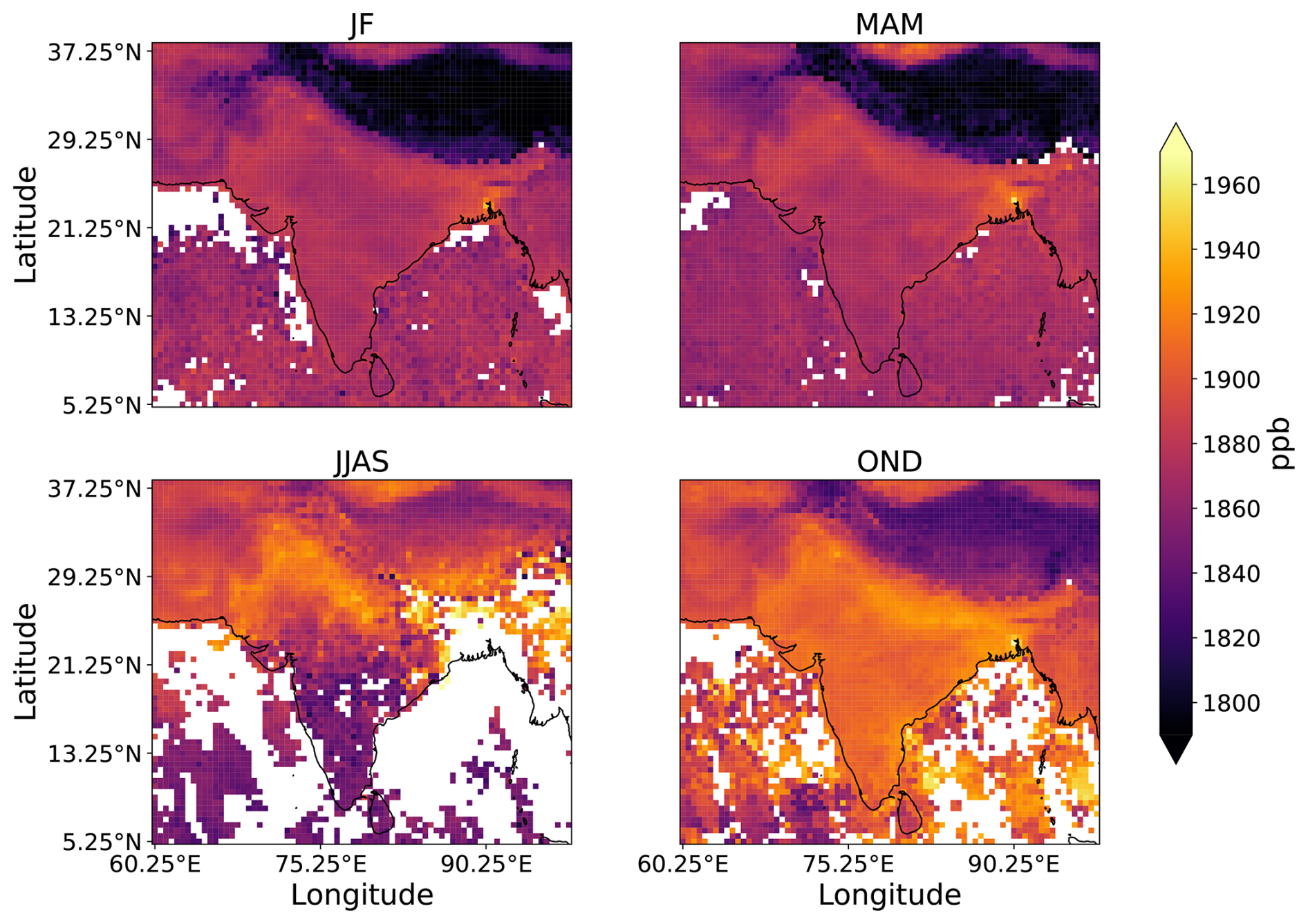
Figure 1 Seasonal mean TROPOMI methane column-averaged dry air mole fractions (XCH₄), averaged over 0.5° × 0.5° grid cells over South Asia. White areas indicate grid cells without observations due to cloud cover and missing retrievals over the ocean.

The data over the study domain (5 to 38° N and 60 to 98° E) comprises approximately 10 000 to 80 000 soundings per day for the year 2020, with a maximum number in November and December and a minimum from June to September (JJAS). The poorer data coverage in the JJAS period is due to the presence of monsoonal clouds. Figure 1 shows the spatial distribution of valid TROPOMI observations across the study domain for the four seasons winter (JF), pre-monsoon (MAM), monsoon (JJAS) and post-monsoon (OND). The retrieved XCH₄ mole fractions are highest from June to December, and the largest values are detected over northern and eastern parts of India, Pakistan and Bangladesh.

Selection of Observation

We only used satellite retrievals flagged as good quality (quality flag = 0). In addition, the column observations over the Himalayan mountains are also excluded because the highly variable topography makes the retrievals more uncertain. Figure 2a shows a time series of monthly mean TROPOMI observed XCH₄ over the study domain. The second half of the year has higher methane mole fractions, likely reflecting increased methane emissions due to the agricultural practices and inundation of wetlands after the monsoon rainfall. The total number of retrievals for the whole domain in 2020 after filtering amounts to approximately 9 million. This vast amount of data would add a prohibitive computational load for the models used in the study, while often delivering redundant information. In order to reduce the number of observations while preserving most of the information content, the retrievals are aggregated and averaged spatially on a 0.25° × 0.25° and a 0.50° × 0.50° latitude/longitude variable grid based on the spatial variability of methane mole fractions in individual retrievals, following the method of Thompson et al. (2025). Essentially, the mean and standard deviation of the column mole fractions in individual retrievals are calculated at the coarsest grid box (0.5°). When the standard deviation in the coarsest grid exceeds a certain threshold (15 ppb), the grid is further divided into a finer grid. This stepwise approach is done to ensure that the grid cells with a higher variability of methane mole fractions are separately taken into account. An example of such a variable grid is shown in Fig. 2b. This method is explained in detail in Thompson et al. (2025), and the aggregated observations from now are called super-observations.

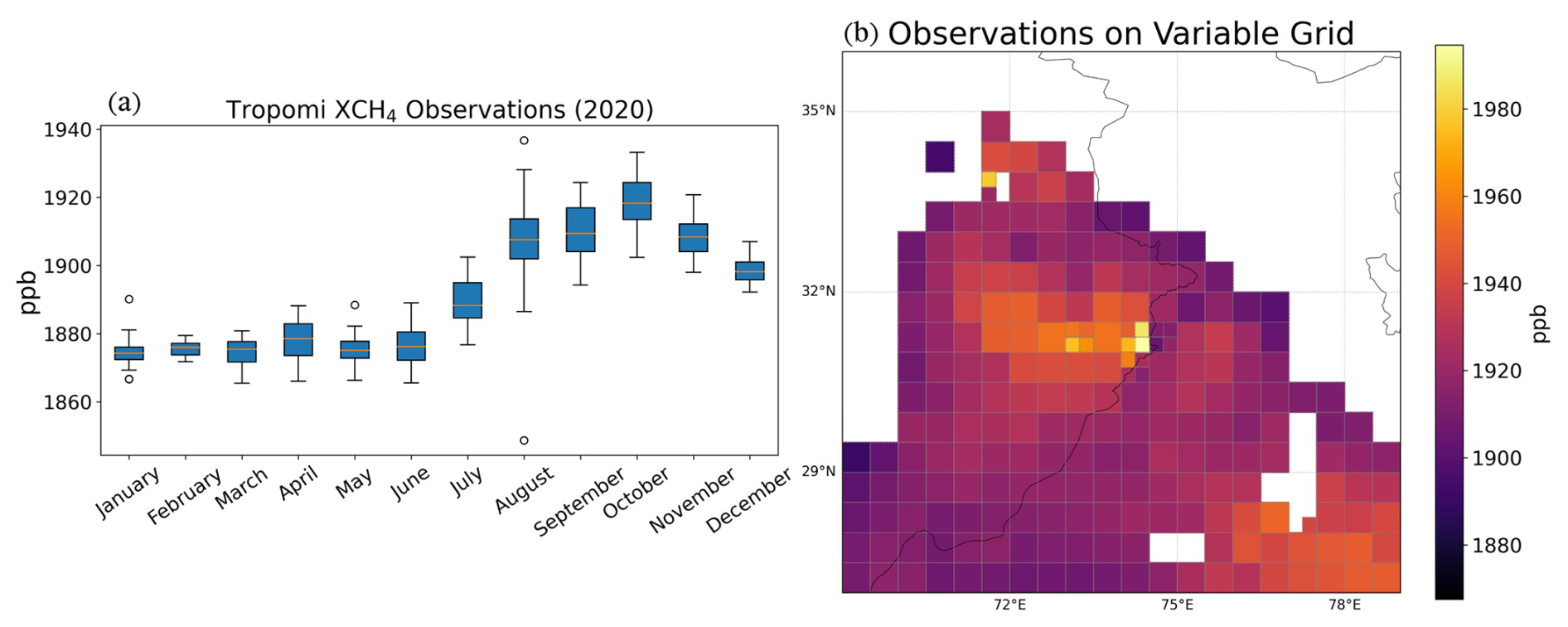
Figure 2 (a) Seasonality of the observed TROPOMI methane column mole fractions (XCH₄) averaged over the whole domain. The blue boxes represent the interquartile range (IQR), the center line the median, the whiskers represent the most extreme data points within 1.5 × IQR of the monthly mole fractions and the circles are outliers. Also shown is the number of retrievals in each month (orange line). (b) Observations aggregated on a variable resolution latitude/longitude grid (0.25° × 0.25° and 0.50° × 0.50°) for a typical day in October. The black circle shows a region where the fine grid is used with larger heterogeneity in mole fractions.

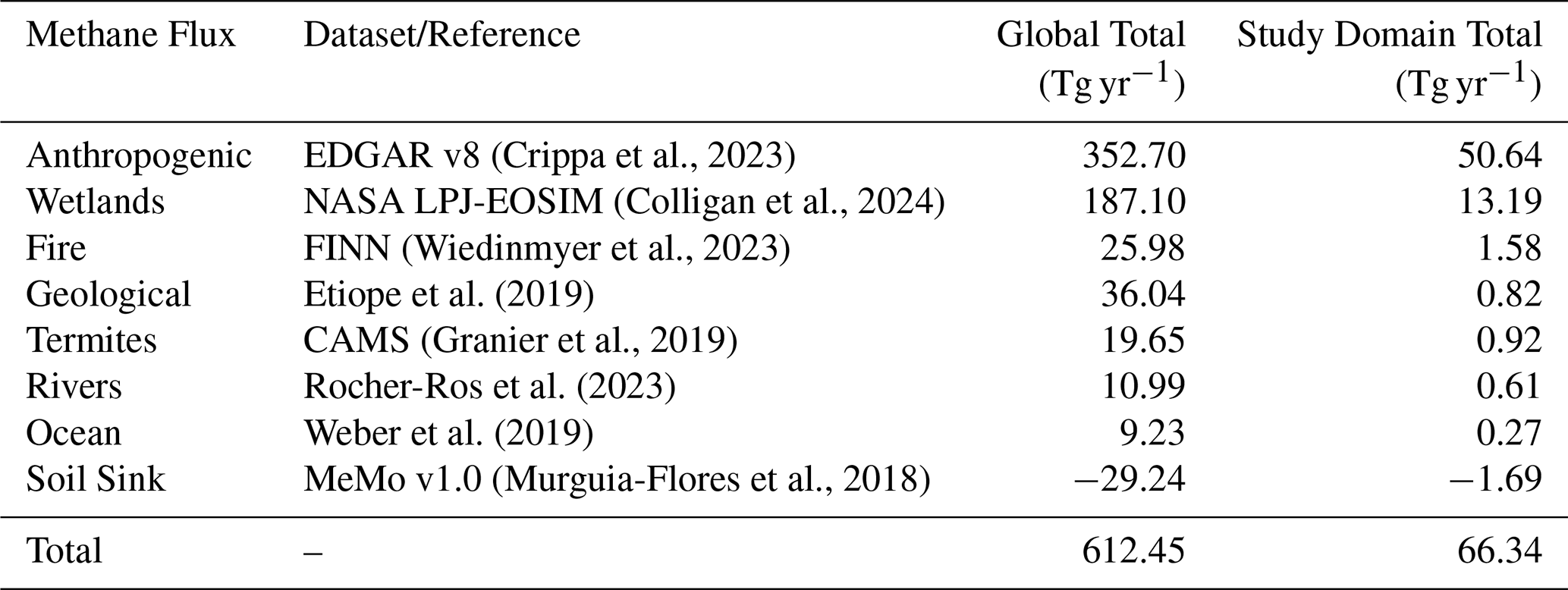
Table 1 Total methane fluxes for the eight sectors used to construct our a priori emissions for the year 2020 globally and for our study domain (5 to 38° N, 60 to 98° E).

2.2 Methane Prior Fluxes

To supply the inversion system with prior methane fluxes, we used bottom-up inventories for eight different source categories: (1) anthropogenic emissions from EDGAR version 8 (Crippa et al., 2023), (2) wetland emissions from the NASA Earth Observation SIMulator version of the Lund-Potsdam-Jena Dynamic Global Vegetation Model – LPJ EOSIM (Colligan et al., 2024), (3) fire emissions from FINN (Wiedinmyer et al., 2023), (4) geological emissions (Etiope et al., 2019), (5) termite emissions from CAMS (Granier et al., 2019), (6) emissions from rivers and streams (Rocher-Ros et al., 2023), (7) shallow coastal water ocean emissions (Weber et al., 2019), and (8) soil sink from the Soil Methanotrophy Model – MeMo v1 (Murguia-Flores et al., 2018). Annual mean maps of all these fluxes are shown in Fig. 3 and total numbers are reported in Table 1. The sums of the fluxes from all source categories were provided to the model at a spatial resolution of 0.5° × 0.5° and at monthly time steps. The net global total methane flux from all these sectors together is 612.5 Tg yr⁻¹, of which 66.3 Tg yr⁻¹ are emitted in the study region (5 to 38° N and 60 to 98° E). A breakdown of the methane flux sources reveals that anthropogenic sources dominate the emissions over the study domain, contributing 50.64 Tg yr⁻¹, which accounts for over 76 % of the total regional methane budget of 66.3 Tg yr⁻¹. The sub-sectors of anthropogenic emissions include mainly agriculture emissions (33.7 Tg yr⁻¹) and waste emissions (10.3 Tg yr⁻¹) followed by fuel production and usage in industries, transport and buildings (Fig. S2 in the Supplement). Wetlands contribute 13.2 Tg yr⁻¹, making them the largest natural source of methane in the region. Other sources such as fires (1.6 Tg yr⁻¹), geological sources (0.8 Tg yr⁻¹), and termites (0.9 Tg yr⁻¹) contribute smaller but non-negligible portions to the total emissions. Emissions from rivers (0.6 Tg yr⁻¹) and oceans (0.3 Tg yr⁻¹) are relatively minor, while the soil sink (−1.7 Tg yr⁻¹) represents a modest removal flux.

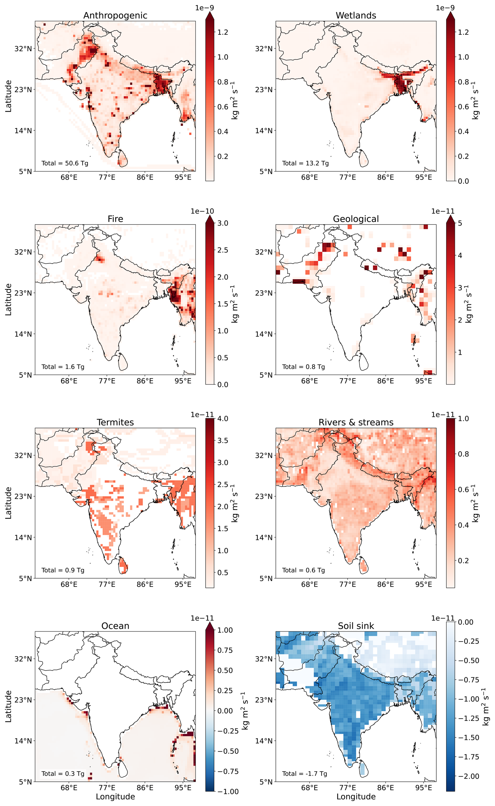
Figure 3 Annual mean bottom-up methane fluxes for the eight sectors used to construct our a priori emissions for the year 2020.

The spatial distribution of these fluxes shows anthropogenic emissions are dominant over the river plains of north-eastern India, Bangladesh and Pakistan. Bangladesh also has high wetland emissions. Notably high landfill emissions can also be found over Islamabad, Delhi, Mumbai, Ahmedabad and Bangalore (Dogniaux et al., 2025; Toha et al., 2025).

2.3 Background Mole Fractions

Methane observed at any location is a combination of local emissions and contributions transported from distant regions, the latter is commonly referred to as the background mole fraction. We calculate the modeled background mole fraction as two components: (1) contribution of methane mole fractions present at the endpoints of the particle trajectories – called the initial mole fraction, (2) contribution from the methane fluxes outside the study domain – from here onwards termed as boundary mole fractions. In our study, the transport modeling (see Sect. 2.4) covers only 20 d backward from every observation. So, the methane present in the atmosphere before that time is accounted for in the initial mole fraction.

To generate the initial mole fraction field for the inversion, we evaluated two different global methane mixing ratio products for their consistency with the TROPOMI observations. The evaluation was performed by co-locating their column-averaged mole fraction with the satellite retrievals. Among the tested datasets, the CAMS global inversion-optimized mole fraction product (v20r1) (Copernicus Atmosphere Monitoring Service, 2020) showed a systematic negative bias relative to TROPOMI, whereas the EGG4 reanalysis dataset (Agustí-Panareda et al., 2023) shows substantially smaller mean bias. Further, when calculating the background mole fractions over the study region by coupling with transport model sensitivities (see Sect. 2.4), the CAMS-based background column mole fractions are typically 30–80 ppb lower than the corresponding TROPOMI XCH₄ values (Fig. S3). As EGG4 assimilates atmospheric methane observations and includes bias correction procedures, it provides a background field that is more consistent with the TROPOMI observations. We, therefore, adopted EGG4 as the initial mole fraction field for the inversion. To further account for uncertainties in the background, we applied a relative background error of 0.3 %–0.7 % in the inversions, corresponding to the order of magnitude of the Root Mean Square Deviation (RMSD) of EGG4 against TROPOMI (∼ 5 ppb), and ensuring consistency between the assumed error and the observational bias characteristics.

2.4 Transport Modeling

This study uses the Lagrangian Particle Transport model – FLEXPART v10.4 to calculate the sensitivity of the column-averaged dry air methane mole fractions to the emission fluxes and background mole fractions. For this, the model is run in backward mode for 20 d from the time of the observations using ERA5 meteorology available at 0.5° × 0.5° resolution. The sensitivity of the simulated column at the receptor to emission fluxes is called Source-Receptor Relationship (SRR) (Seibert and Frank, 2004), and the sensitivity to the initial mole fraction field at the trajectory end points is called Background-Receptor Relationship (BRR). The SRRs and BRRs were calculated at 0.5° × 0.5° resolution for the study domain (5 to 38° N and 60 to 98° E) and at 2° × 2° globally, and include sensitivity reductions due to chemical reaction with the hydroxyl radical.

Methane mixing ratios can be modeled with FLEXPART using:

$$\begin{array}{}\text{(1)}& {\mathit{y}}^{\mathrm{model}}=\mathbf{H}\mathit{f}+{\mathbf{H}}^{\mathrm{ini}}{\mathit{y}}^{\mathrm{ini}}\end{array}$$

where y^model is the model mole fraction, H is the sensitivity to emission fluxes (SRR), Hⁱⁿⁱ is the sensitivity to initial mole fractions (BRR), f are the a priori fluxes, and yⁱⁿⁱ are the background mole fractions. Here, the first term (Hf) is the contribution from fluxes to the modeled CH₄ total column, and the second term (Hⁱⁿⁱyⁱⁿⁱ) is the contribution from the initial mole fraction. For modeling total column mixing ratios, Thompson et al. (2025) introduced an efficient framework that accounts for the averaging kernel used in the satellite retrieval. We follow their methodology and, thus, give only a short description. To compare the model and satellite retrievals, we need to consider the effect of the retrieval kernel on the model column mole fraction. The layer-wise scalar form of model column mole fraction is:

$$\begin{array}{}\text{(2)}& x^{\mathrm{avg}}=x^{\mathrm{pri}}+{\sum }_{n=\mathrm{1}}^N{a}_n\left(x_n^{\mathrm{model}}-x_n^{\mathrm{pri}}\right)w_n\end{array}$$

where x^avg is the model column average mole fraction, x^pri is the prior column mole fraction used in the satellite retrieval, a_n is the averaging kernel sensitivity at layer n, $x_n^{\mathrm{model}}$ is the model mole fraction at layer n, $x_n^{\mathrm{pri}}$ is the prior mole fraction at layer n, w_n is the pressure weighting term, and N is the total number of vertical layers used in the satellite retrieval. A total of 30 000 particles were released per retrieval column. Inserting Eq. (1) into Eq. (2) leads to:

$$\begin{array}{}\text{(3)}& x^{\mathrm{avg}}=x^{\mathrm{pri}}+{\sum }_{n=\mathrm{1}}^N{a}_n\left({\mathbf{H}}_n\mathit{f}+{\mathbf{H}}_n^{\mathrm{ini}}{\mathit{y}}_n^{\mathrm{ini}}-x_n^{\mathrm{pri}}\right)w_n\end{array}$$

Here, a_n, w_n and $x_n^{\mathrm{pri}}$ are scalar layer-dependent quantities, while H_n and ${\mathbf{H}}_n^{\mathrm{ini}}$ denote linear transport operators mapping fluxes and background mole fractions to the contribution from retrieval layer n. The term, Σa_nH_nw_n is the total column SRR. The calculation of column SRRs relies on sampling particles in a grid cell and summing their contributions according to the retrieval layer from which they were released. While, in principle, one could retain information on the specific retrieval layer each particle originated from, Thompson et al. (2025) showed that it is much more efficient to represent the information of the averaging kernel and pressure weighting (a_nw_n) in the particle density at the initialization of the particle release. As such, the number of particles release per layer is varied according to p_n=pa_nw_n, where p is the total number of particles released per retrieval. This means that the information from which layer a particle originated does not need to be kept and this formulation leads to a simplified expression equivalent to that used for point observations. Figure 4 illustrates a sample distribution, showing how the averaging kernel and pressure weighting determine the vertical distribution of particles across the retrieval layers. The results are numerically consistent with the full layer calculation but require substantially less computation, making it possible to treat total column observations with the same efficiency as point measurements. More details on this method can be found in Thompson et al. (2025).

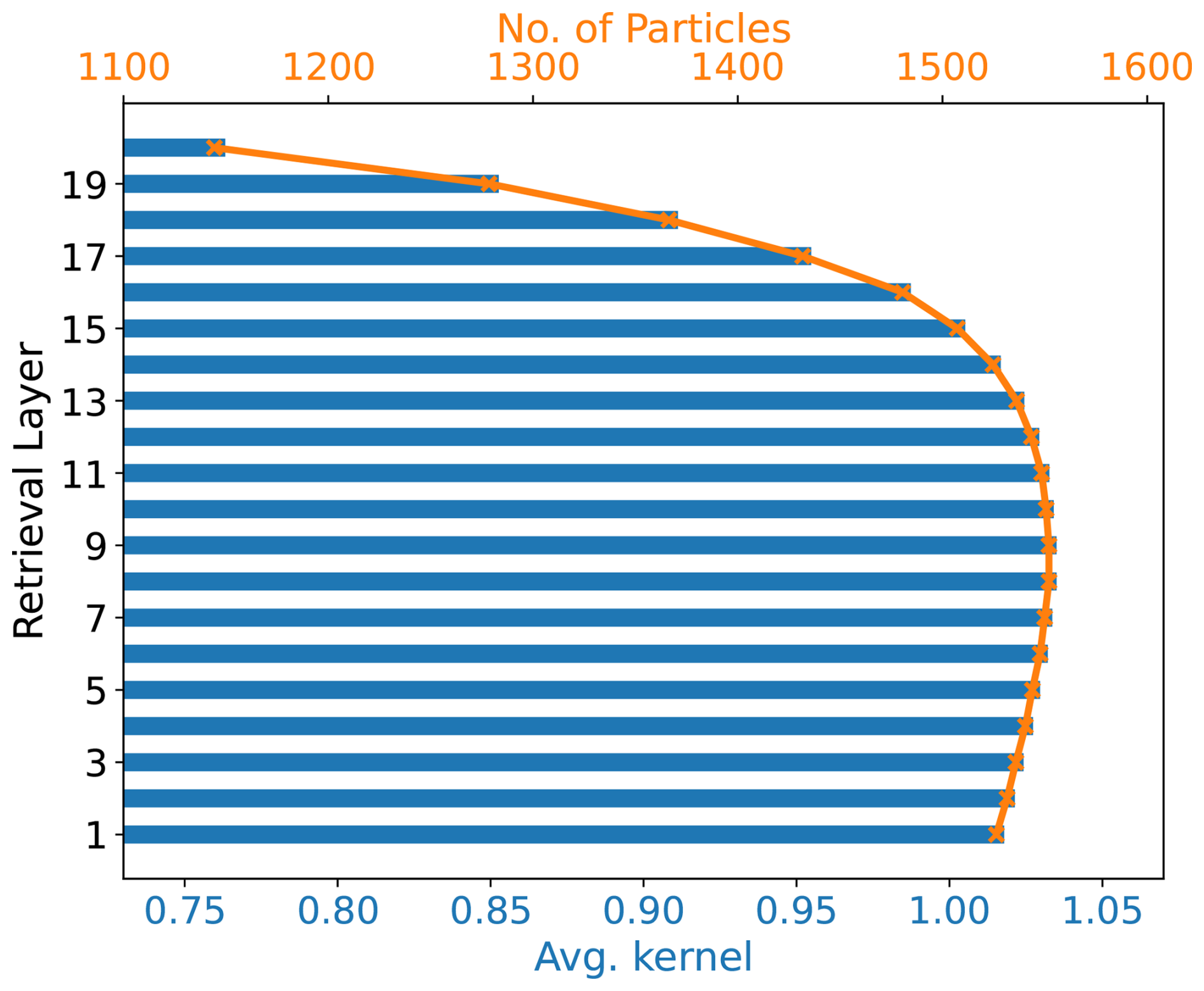
Figure 4 Vertical distribution of particles for a sample retrieval. Blue bars show the averaging kernel values for each retrieval layer, and the orange line indicates the corresponding number of particles released per layer after weighting by the averaging kernel and pressure term.

2.5 Inverse Modeling

The Bayesian inversion method (Tarantola, 2005) corrects the prior flux estimates based on the available observations, while accounting for uncertainties in both the measurements and the modeling system. This study employs the Bayesian inverse modeling system – FLEXINVERT (Thompson and Stohl, 2014) to optimize the methane emissions across South Asia. Here, we used the sensitivity fields derived from transport modeling to quantify the influence of surface emissions to the satellite-observed methane mole fractions, represented as the transport operator H. The inversion then adjusts the prior fluxes to minimize the mismatch between the modeled and observed mole fractions, resulting in posterior fluxes that are more consistent with the atmospheric measurements. This is formulated as a cost function J(x) that balances deviations from both prior emissions and observational constraints. The cost function is defined as:

$$\begin{array}{}\text{(4)}& \begin{array}{rl}J\left(\mathit{x}\right)=& {\displaystyle \frac{\mathrm{1}}{\mathrm{2}}}{\left(\mathit{x}-{\mathit{x}}_{\mathrm{b}}\right)}^T{\mathbf{B}}^{-\mathrm{1}}\left(\mathit{x}-{\mathit{x}}_{\mathrm{b}}\right)\\ & +{\displaystyle \frac{\mathrm{1}}{\mathrm{2}}}(\mathit{y}-\mathbf{H}\mathit{x}{)}^T{\mathbf{R}}^{-\mathrm{1}}(\mathit{y}-\mathbf{H}\mathit{x})\end{array}\end{array}$$

where x_b is the state vector of prior fluxes, y is the observation vector, H is the transport operator, B and R are the error covariances associated with the prior errors and observation errors. The state vector is optimized at a 30 d temporal resolution and at spatial resolutions ranging from 0.5 to 2.0°, depending on how strongly emissions in a region influence the observations. The inversion was restricted to land regions, with only terrestrial fluxes being optimized. The state vector further contains scalar parameters for the initial mole fraction field. These are specified across four latitude bands (90–30° N, 30–0° N, 0–30° S, and 30–90° S) and three vertical layers (0–2000, 2000–10 000, and 10 000–50 000 m above ground level), and are optimized on a 30 d timescale. We used a range of prior and background uncertainties for the inversions (see Sect. 3.1). For the reference inversion, a prior flux uncertainty of 100 % and a background uncertainty of 0.3 % are assumed. The prior error covariance matrix B is constructed by assigning the variance in each grid cell as the square of its prior uncertainty, while the covariances were defined using an exponential decay function with a correlation length of 250 km between grid cells. In addition, temporal correlations were accounted for using an exponential decay with a correlation timescale of 30 d. Observation errors were derived from the TROPOMI retrieval uncertainties. For each super-observation, the uncertainty was computed as the root-sum-square of the individual retrieval uncertainties, weighted by their respective ground pixel areas. The total observation space uncertainty includes both the super-observation error and the error from background mole fractions. This uncertainty corresponds to an IQR of 14–18 ppb with a mean of 16 ppb. The squares of these uncertainties were used as the variances in the observation error covariance matrix R. The errors in the super-observations were assumed to be uncorrelated. The cost function for the inversion can be solved either numerically or analytically. This study employs an analytical solution for inversions:

$$\begin{array}{}\text{(5)}& {\mathit{x}}_{\mathrm{a}}={\mathit{x}}_{\mathrm{b}}+{\left({\mathbf{B}}^{-\mathrm{1}}+{\mathbf{H}}^T{\mathbf{R}}^{-\mathrm{1}}\mathbf{H}\right)}^{-\mathrm{1}}{\mathbf{H}}^T{\mathbf{R}}^{-\mathrm{1}}\left(\mathit{y}-\mathbf{H}{\mathit{x}}_{\mathrm{b}}\right)\end{array}$$

where x_a is the posterior estimate.

3 Inversion Results and Evaluation

3.1 Results and Discussion

Figure 5 shows the agreement between observed and modeled column-averaged methane mole fractions before and after the inversion. This plot gives a comprehensive view of the performance of the inversion system. The correlation coefficient increases from 0.65 (prior) to 0.89 (posterior), indicating a substantial improvement in the posterior estimates after assimilating the satellite observations. With the prior emissions, the slope between the model and the observations is 0.86 and there is a large positive intercept of 262 ppb. With the posterior emissions, the slope is close to 1 and the intercept nearly zero, indicating an almost unbiased fit. This validates that the posterior emissions better reproduce the observed atmospheric mole fractions, demonstrating the effectiveness of the inversion. However, since this validation is not against independent data, this shows only that the inversion is performing as expected.

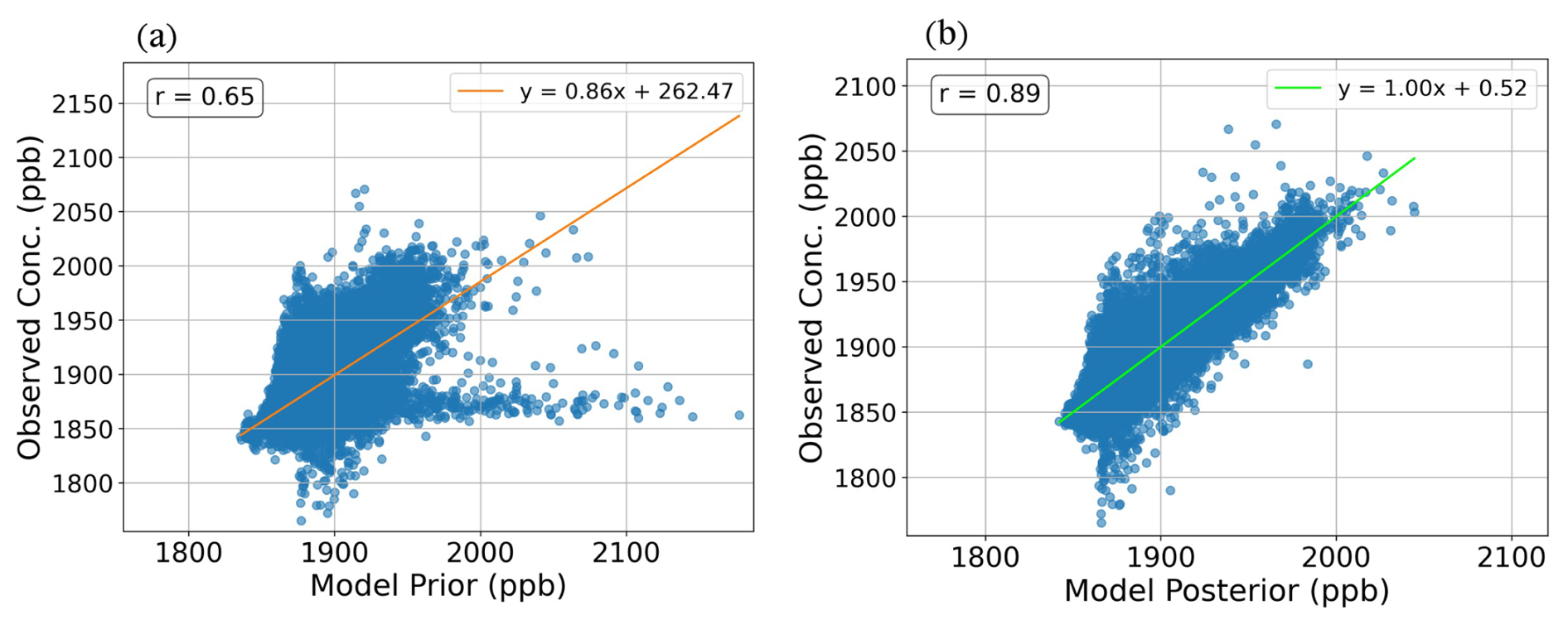
Figure 5 Scatter plot of observed TROPOMI CH₄ column-average mole fractions against FLEXPART model estimates over South Asia, (a) with prior and (b) with posterior emissions.

The South Asian region experiences a distinct seasonal pattern characterized by wet summers and dry winters. During summer, from June to September, strong south-westerly winds prevail due to the South Asian monsoon, while winter is dominated by dry continental winds predominantly from the north-east.

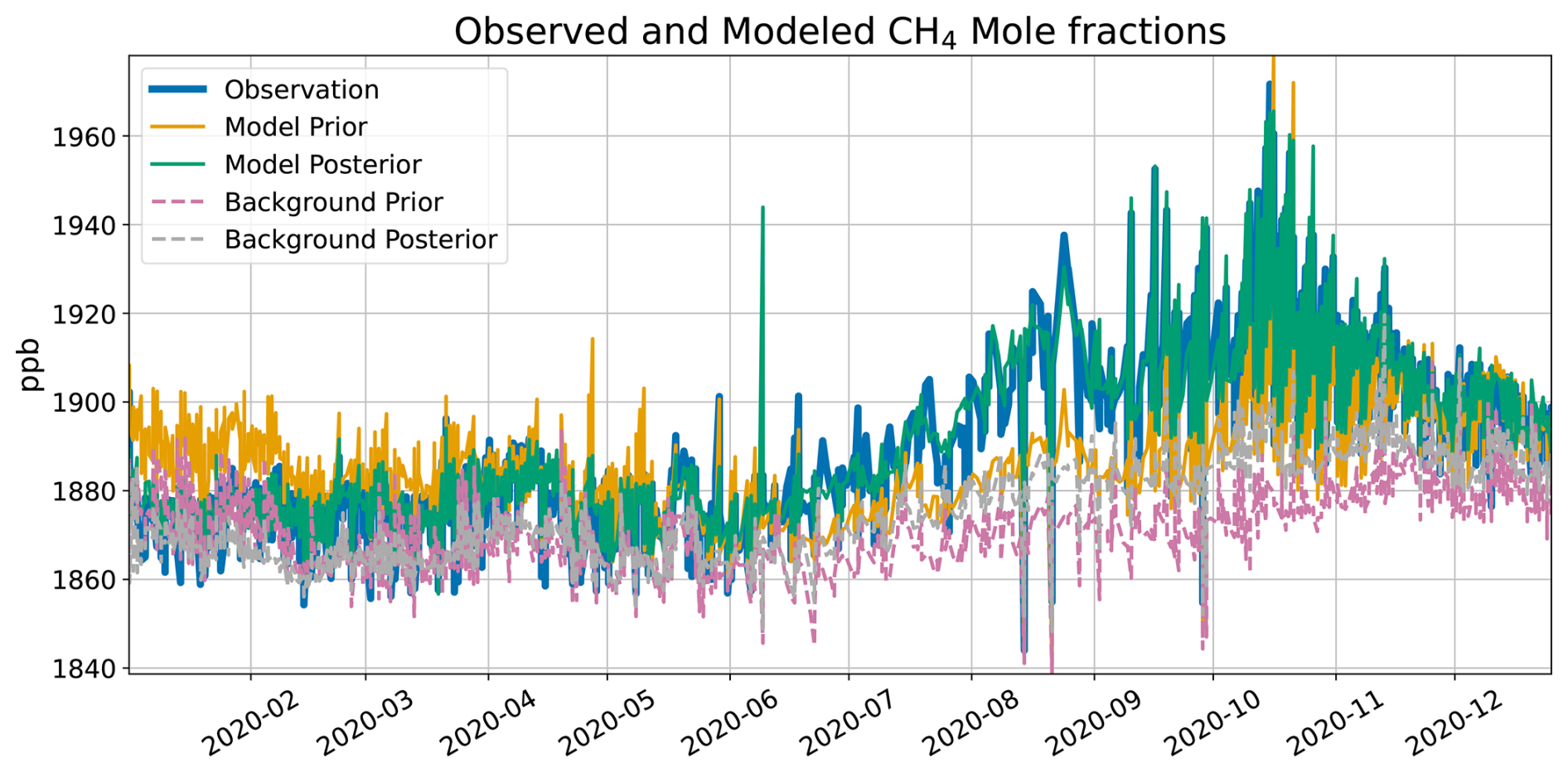
Figure 6 Time series of observed and modeled prior and posterior methane (CH₄) column-averaged dry air mole fractions averaged over South Asia. Modeled prior and posterior background are also shown.

Figure 6 shows the time series of the spatially averaged observed and modeled column-average mole fractions of CH₄ for the reference inversion. The TROPOMI observations (blue line) show a strong increase in column-average CH₄ dry air mole fractions during and after the monsoon season. The prior background mole fractions (dashed purple line) are higher from October to February, due to the northerly winds carrying air which is enriched in CH₄, and lower from June to September, due to the cleaner air arriving from the Southern Ocean during the monsoon season (the slight increase in the domain-averaged background seen in Fig. 6 during this period likely reflects enhanced CH₄ over the northwestern part of the domain, where transport is more locally influenced). Our inversion simultaneously optimizes both the background methane mole fractions and the prior emissions. The posterior background mole fractions (dashed grey line) are adjusted downward during January to May and upward from June. The model prior mole fractions (orange line) significantly overestimate the observations during the dry months from January to May and underestimate them during the wet period from June to September. The posterior mole fractions (green line) show the inversion's ability to bring the simulated values closer to the observations. While this is partly due to a correction of the background values, a substantial portion of the correction is due to increased emission contributions from South Asia during June to September (Fig. 8). These results indicate that the bottom-up inventories misrepresent the seasonal dynamics of methane emissions in South Asia.

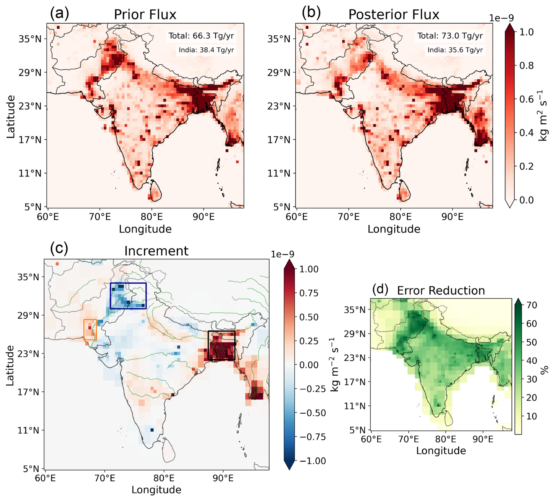
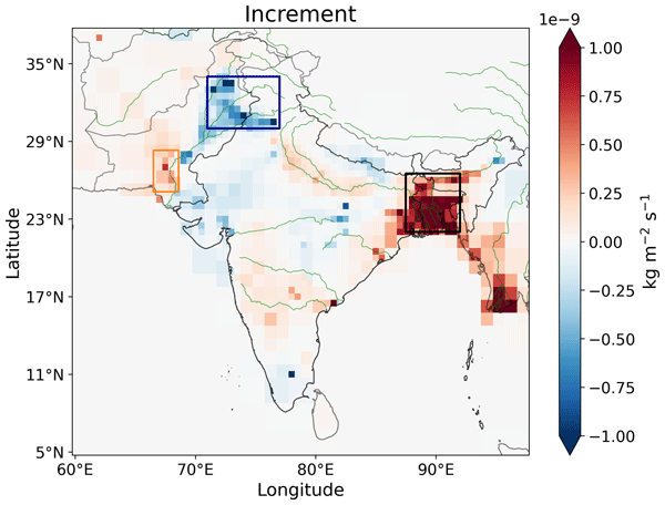
Figure 7 Spatial distribution of (a) prior and (b) posterior methane emission and their increments (c) (posterior minus prior) across South Asia for the year 2020. Positive values (red) indicate regions where emissions were underestimated in the prior inventories, while negative values (blue) indicate overestimation. The three marked boxes highlight regions of interest discussed in the text. Major river systems (Indus, Ganges, and others) are overlaid in green for geographical context. Panel (d) shows the uncertainty reduction across the region.

Table 2 Prior and posterior methane emission estimates (Tg yr⁻¹ CH₄) for South Asia and individual countries in 2020. The inversion increases the regional total from 66.34 ± 6.65 to 73.01 ± 0.70 Tg yr⁻¹, with the largest upward adjustment over Bangladesh (+5.6 Tg yr⁻¹), while India shows a reduction of −2.8 Tg yr⁻¹. Smaller contributions come from Afghanistan, Bhutan, Sri Lanka, and Nepal (ABSN).

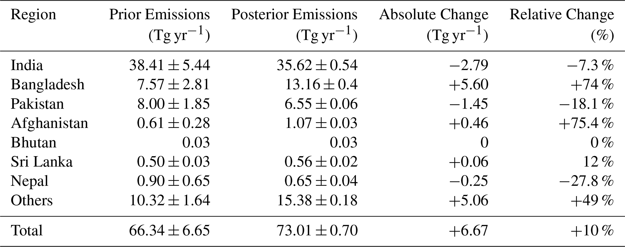
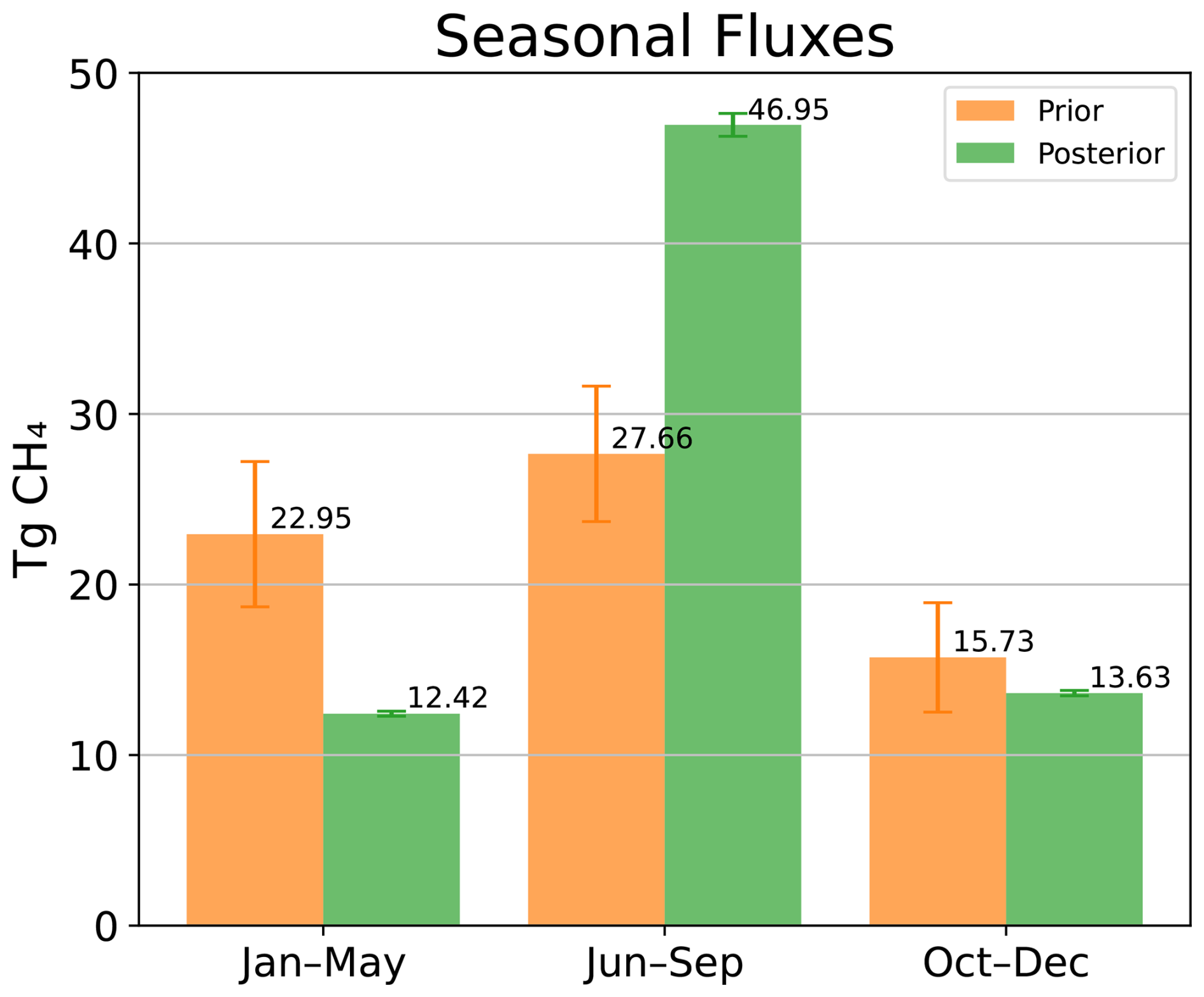
Figure 8 Seasonal methane fluxes (Tg CH₄) over South Asia for three periods (January–May, June–September, October–December), comparing prior fluxes (orange bars) with posterior fluxes (green bars). Error bars indicate the corresponding uncertainty ranges.

Figure 7a–b shows the spatial distribution of the prior and posterior methane fluxes and Table 2 provides a summary of the methane emissions for the different countries. The prior methane emissions from South Asia as a whole are 66.34 ± 6.65 Tg yr⁻¹, with the top three emitters India, Bangladesh and Pakistan contributing 38.41 ± 5.44, 7.57 ± 2.81, and 8.00 ± 1.85 Tg yr⁻¹, respectively. The countries Afghanistan, Bhutan, Sri Lanka and Nepal (referred to as ABSN from here onwards) together contribute only 2.04 Tg yr⁻¹. Myanmar, which is only partially in our inversion domain, contributes a total of 10.3 Tg yr⁻¹.

The inversion gives a total posterior methane flux of 73.01 ± 0.70 Tg yr⁻¹, 6.7 Tg yr⁻¹ more than the prior estimate. Of this, India accounts for 35.62 ± 0.54 Tg yr⁻¹ (a reduction of 7 % from the prior), Bangladesh for 13.16 ± 0.4 Tg yr⁻¹ (an increase of 74 %) and Pakistan for 6.55 ± 0.06 Tg yr⁻¹ (a reduction of 18 %), respectively. Bangladesh accounts for the majority of the regional increase. The posterior emissions from ABSN countries, 2.30 Tg yr⁻¹ (an increase of 13 %) remain relatively minor. The posterior flux uncertainties reported here are obtained from the error propagation in the analytical inversion and, therefore, represent the formal Bayesian uncertainties. However, they may not fully capture the real uncertainty in the posterior fluxes, particularly for aggregated regional or annual totals.

Figure 7c shows the spatial distribution of the increments in the methane fluxes after the inversion (posterior − prior) overlaid with major rivers in the region. Areas dominated by wetlands and agriculture (Figs. 3 and S2) show the strongest posterior-prior differences. The majority of these positive increments were observed in the eastern Indo-Gangetic Plain and Bangladesh. This region, marked with a black box (22–26.5° N, 87.5–92° E) in Fig. 7c, alone has a posterior emission of 20.83 Tg yr⁻¹ of methane (∼ 30 % of total domain emission), representing an increase of +8.4 Tg yr⁻¹ from prior emissions. This indicates that inventories substantially underestimate emissions in these densely irrigated and wetland-rich areas. Given its significant contribution, this region is a key focus of our study and is examined in more detail later in this section. The positive increments in the north-western India clearly align with the trajectory of the river Yamuna and Ganges, indicating uncaptured emissions in inventories, possibly from the agriculture sector. Several studies have shown rice cultivation as a key contributor to methane emissions in this region (Anand et al., 2005; Gupta et al., 2015; Manjunath et al., 2006; Matthews et al., 1991) due to the use of nitrogen fertilizers, organic manure, and livestock population (Singh et al., 2021).

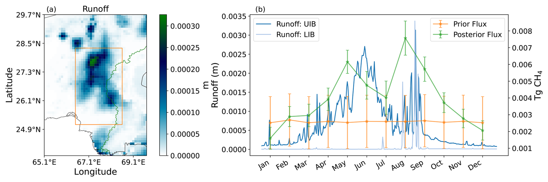
Figure 9 (a) Spatial distribution of annual runoff from ERA5-Land in the Lower Indus Basin (LIB), with the orange box indicating the analysis area. (b) Monthly mean methane fluxes (prior in orange, posterior in green) in the LIB compared with runoff time series for both the upper and lower Indus Basin. The posterior fluxes capture a clear seasonal cycle with peaks in May and August, consistent with runoff variability, showing a similar pattern to runoff variability in the basin.

Most of the negative adjustments are seen over western India and Pakistan. A comparison with the prior flux maps (Fig. 3) shows that these are mostly agricultural and waste-related emissions in the prior (Fig. S2). In the Upper Indus Basin region (blue box), emission estimates are reduced by −2.4 Tg yr⁻¹, suggesting that bottom-up inventories overestimate fluxes in these sparsely monitored regions. While the total methane emissions in Pakistan decrease overall after the inversion, the region (marked with an orange box) within the Lower Indus Basin (LIB) shows an increase of 0.5 Tg yr⁻¹. A closer examination at this region reveals that, when the prior fluxes show an almost flat seasonal cycle, the posterior fluxes capture a distinct seasonality with peaks in May and August (Fig. 9b). This region is periodically wetted by the Indus River, whose flow is governed by both natural processes – such as glacier and snowmelt from the northern mountains and monsoonal rainfall – and strong human regulation through irrigation and agricultural diversions, particularly within the LIB. Previous studies, such as Baig et al. (2022), have also reported a comparable dual-peak seasonality in river discharge in the Upper Indus Basin (UIB), driven by glacier melt, snow and rainfall contributions. To examine this further, we analyzed runoff data from ERA5-Land (Muñoz-Sabater et al., 2021), which combine surface and subsurface components resulting from rainfall, melting snow, and soil drainage. The analysis reveals a strikingly similar spatial pattern in annual runoff (Fig. 9a) to the flux increments seen in the orange-box region. The runoff data also exhibit a dual-peak cycle in the UIB, with maxima in June and September, while the lower Indus Basin shows only a single pronounced peak in August (Fig. 9b). This difference likely reflects the strong influence of the Indus Basin Irrigation System, where extensive human regulation and diversion for irrigation and agriculture modify the natural water flow (Janjua et al., 2021), a process that may not be represented accurately in the river flow datasets (Liu et al., 2018). The posterior methane fluxes in Fig. 9b tend to peak slightly earlier than the corresponding runoff peaks, indicating a temporal lag between runoff data and methane emissions. This may be due to known uncertainties in Indus discharge data, where mean annual biases of about 22 % and monthly errors exceeding 200 % have been reported (Liu et al., 2018), potentially distorting both the timing and magnitude of seasonal peaks. Such discrepancies are further amplified downstream by barrage operations and canal withdrawals in the Indus Basin Irrigation System (Bhatti et al., 2019), while long-term analyses also indicate a progressive shift toward earlier streamflow timing (Ali et al., 2023). Further, the grid cell encompassing Karachi, Pakistan, shows a positive posterior increment, with highest posterior methane emissions in September. Although this timing coincides with the late-monsoon period and Karachi flooding in 2020, given the large uncertainties at the grid-cell scale and the limited temporal coverage, no direct attribution to individual hydrometeorological events can be made.

The year 2020 marked an above-normal monsoonal rainfall in South Asia, with India receiving 109 % of its Long Period Average (LPA). This marked the second consecutive year of above-normal monsoon rainfall in India, following 2019's 110 % of LPA – a pattern not observed since 1958 and 1959. Concurrently, Bangladesh faced historic flooding, with approximately a quarter of the country submerged. Almost a million homes were inundated, and more than 1500 km² of farmland were damaged across the country.

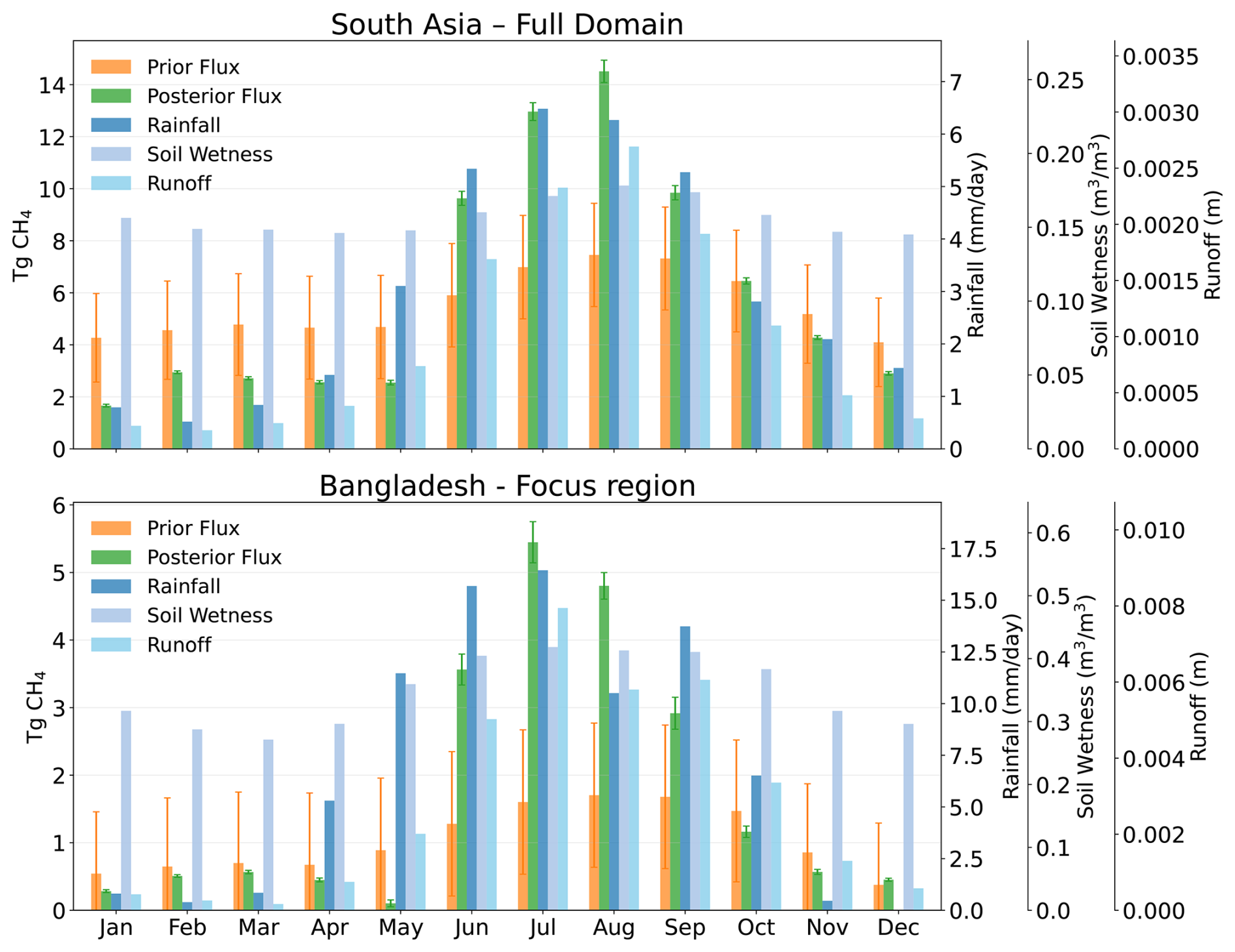
Figure 10 Monthly total prior (blue) and posterior (orange) methane fluxes for the full South Asia domain (top) and the Bangladesh focus region (bottom), shown together with monthly mean rainfall, runoff and soil wetness.

To understand the role of the monsoon in the emissions, their key natural drivers such as rainfall and soil moisture were compared with monthly prior and posterior methane fluxes. Rainfall data is taken from the Global Precipitation Climatology Project (Adler et al., 2017) and soil wetness from ERA5-Land (Hersbach et al., 2018), with the top four layers (∼ 3 m depth) averaged. Figure 10 shows prior and posterior fluxes alongside rainfall and soil wetness for the South Asia full domain (top) and the Bangladesh-focused black box region (bottom). The figure highlights a strong seasonal contrast. During the early part of the year (January–May), the inversion reduced fluxes by 46 % relative to the prior (10.5 Tg). In the monsoon months (June–September), posterior fluxes showed a 70 % upward adjustment (19.3 Tg) (Fig. 8), coinciding with peak rainfall and soil wetness, and reflecting the strong hydrological forcing on emissions. The largest increments occur in July–August, when rainfall and soil wetness reach their maxima. In the post-monsoon period (October–December), posterior emissions were 13 % lower than the prior (2 Tg yr⁻¹), with the retreat of rainfall and soil saturation. The seasonal amplitude is strongest within the box region, consistent with the historic flooding in Bangladesh.

To assess this link statistically, we calculated the spatio-temporal Pearson correlation of methane fluxes before and after the inversion with the hydrological drivers. This analysis revealed that soil wetness shows a correlation of 0.28 with the prior fluxes, which increases to 0.31 after inversion, corresponding to a 25 % rise in the explained variance. For rainfall, the correlation increases from 0.48 to 0.53 (+22 % in explained variance). The rainfall correlation was calculated with a one-month lag to reflect the delayed response of emissions to precipitation-induced inundation. The relationship with runoff strengthens from 0.23 in the prior to 0.32 in the posterior fluxes – an increase of about 94 % in the variance explained. Together, these results suggest that the inversion tends to increase the consistency between methane flux variability and hydrological drivers compared to the prior. While the absolute correlations remain modest and the analysis is limited to a single year, the coherent increases across multiple hydrological variables indicate a plausible hydrological imprint on the posterior fluxes, warranting further investigation using longer time series.

Thus, the strong South Asian monsoon and associated extensive flooding in 2020 appear to have played an important role in driving the positive flux increments in this region. Previous studies such as Peng et al. (2022) identified wetland emissions as the major reason for the 2020 global methane growth. According to NASA Earth Observatory (2023), a substantial fraction of the surge in atmospheric methane in 2020 was driven by wetland emissions. Fueled by the strong South Asian monsoon in 2020, wetlands in Bangladesh and possibly all of South Asia appear to have contributed substantially to this enhancement. Recent assessments (Ciais et al., 2026) attribute a substantial fraction of the increase to reduced OH concentrations, while also highlighting that enhanced emissions from wetlands, inland waters, and agricultural sources contributed significantly to the observed methane rise. Similarly, Niwa et al. (2025) emphasized the role of wetlands and agricultural activities as key drivers of biogenic methane emissions in this region, and Ganesan et al. (2017) highlighted the monsoon-driven seasonal emission cycle over India, with the largest discrepancies between top-down and inventory estimates occurring during the summer season due to rice cultivation. These regions of spatial mismatch between prior and posterior fluxes would be of prime interest for future field campaigns and for improving process models of methane emissions from rice paddies and wetlands, which are essential for reducing uncertainties in emission inventories.

An uncertainty reduction map is calculated as one minus the ratio of posterior to prior uncertainties (Fig. 7d). The inversion could achieve a maximum of 70 % uncertainty reduction in some regions with a median uncertainty reduction close to 40 % in most of the area. The maximum uncertainty reduction is mostly achieved in the regions with higher emissions and higher data coverage.

3.2 Validation

To assess the robustness of the inversion results, lacking surface observations in South Asia, we performed an independent validation using the GOSAT–TROPOMI blended XCH₄ dataset (Balasus et al., 2023). This relatively recent product combines TROPOMI and GOSAT XCH₄ retrievals using a machine-learning bias-correction framework designed to reduce the systematic biases between the two satellite instruments relative to ground truth and to improve spatial consistency. The dataset is publicly available and has already been used in several studies to infer methane emissions. Importantly, it is developed independently of the WFMD TROPOMI retrievals used in our inversion, thereby providing a fully external and independent consistency check of the posterior solution.

Figure 11 shows the time series of domain averaged column mean methane concentrations for 2020, comparing the prior model simulation, the posterior model simulation, and the blended GOSAT–TROPOMI observations. The prior simulation systematically underestimates methane concentrations during the monsoon and post-monsoon months (June–November), while slightly overestimating concentrations during the pre-monsoon period (January–May). This behavior is consistent with the seasonal flux adjustments inferred by the inversion, where prior emissions were found to be too low in the second half of the year and too high in the first half. The posterior simulation shows a clear improvement in capturing both the seasonal amplitude and the temporal variability of the observations, although a slight overestimation is seen overall. In particular, the enhanced concentrations during August-October are much better reproduced after inversion, indicating that the additional emissions inferred during the monsoon season are physically consistent with the observed atmospheric signal.

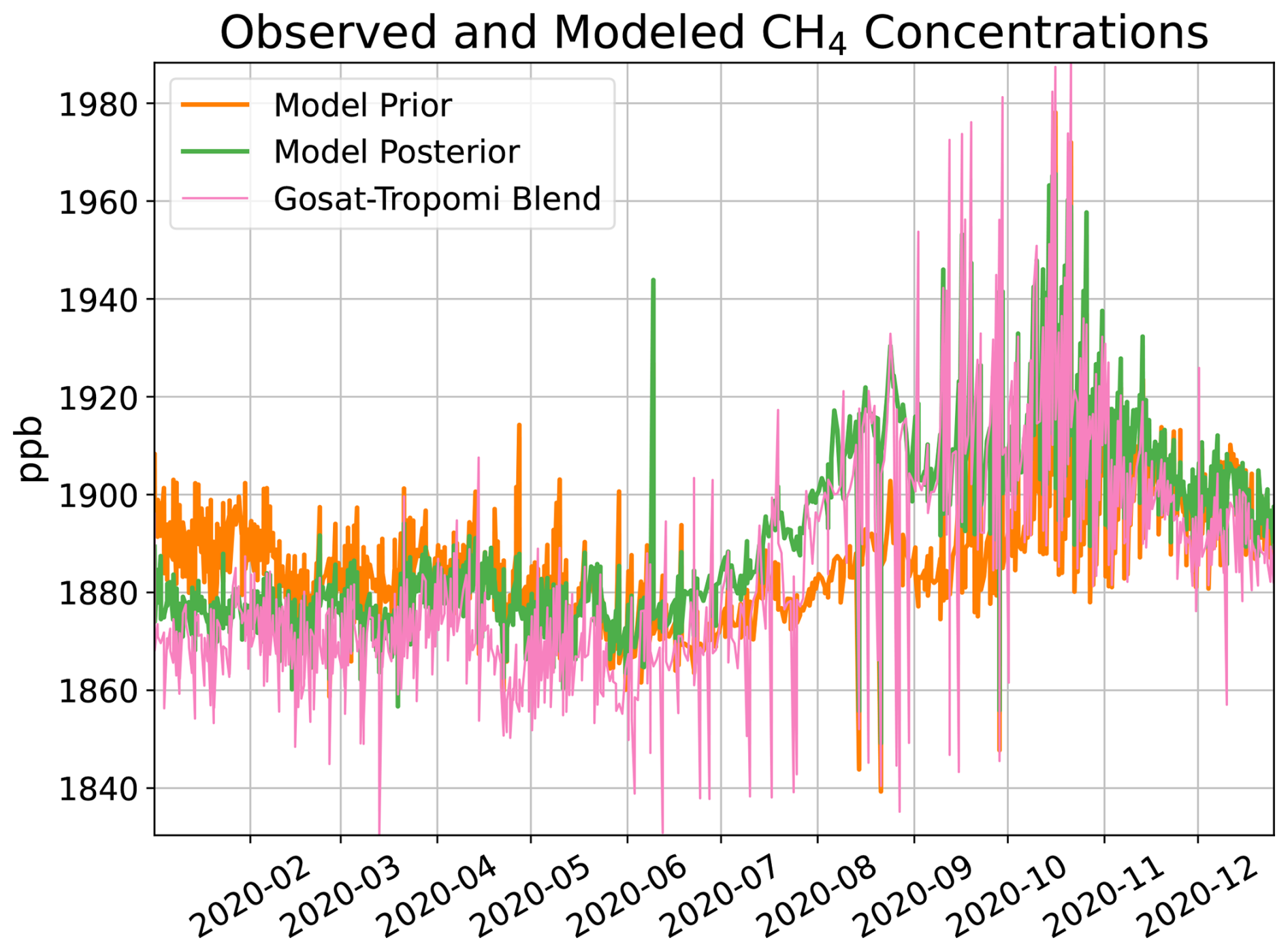
Figure 11 Domain-averaged prior and posterior modeled CH₄ concentrations compared with the GOSAT–TROPOMI blended XCH₄ dataset.

The improvement is further quantified in Fig. 12, which shows the (a) RMSE and (b) MBE between modeled and blended XCH₄ for three seasonal groupings: January–May, June–September, and October–December.

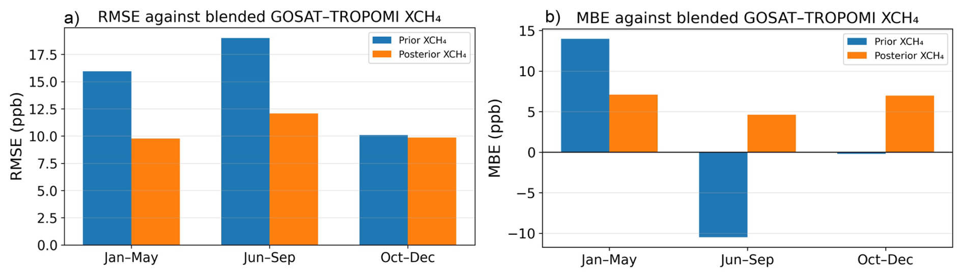
Figure 12 Seasonal RMSE (a) and MBE (b) of prior and posterior modeled XCH₄ relative to GOSAT–TROPOMI blended dataset. Statistics are shown for January–May, June–September, and October–December. The posterior simulation shows reduced errors and seasonal biases compared to the prior.

For January–May, the RMSE decreases from 15.94 ppb (prior) to 9.77 ppb (posterior), corresponding to a reduction of 6.18 ppb or 38.7 %. During the monsoon season (June–September), where the largest seasonal mismatch was observed in the prior simulation, the RMSE decreases from 19.01 to 12.07 ppb, representing a reduction of 6.93 ppb or 36.5 %. This is the largest absolute RMSE improvement and confirms that the inversion effectively corrects the strong underestimation of methane during the monsoon period. For October–December, the improvement is smaller, with RMSE decreasing from 10.09 to 9.86 ppb (a reduction of 0.24 ppb, or 2.3 %), indicating that the prior simulation was already relatively consistent with observations during this period. Overall, the posterior simulation consistently reduces the error relative to the independent blended dataset, with the most pronounced improvements occurring during the monsoon season.

For January–May, the prior simulation shows a strong positive bias of +13.98 ppb, which is reduced to +7.07 ppb in the posterior simulation. This corresponds to a bias reduction of 6.91 ppb (∼ 49 % reduction), indicating that the inversion corrects the prior overestimation during the pre-monsoon season. During June–September, the prior simulation shows a pronounced negative bias of −10.49 ppb, reflecting the underestimation of emissions. After inversion, the bias shifts to +4.61 ppb, reversing the sign of the bias but reducing its magnitude relative to the observations. For October–December, the prior bias is nearly neutral (−0.21 ppb), while the posterior shows a modest positive bias (+6.97 ppb). Although this increases the mean bias during this period, the RMSE remains largely unchanged, indicating that variability is still well represented.

Overall, the independent validation with the blended GOSAT–TROPOMI dataset demonstrates that the posterior solution improves both variance-based (RMSE) and mean-state (MBE) agreement with observations, increasing confidence in the inferred seasonal methane flux corrections.

3.3 Sensitivity to Prior Flux Magnitude

To assess the dependence of the inversion on the assumed prior flux magnitude, we performed a series of sensitivity experiments in which the total prior emissions were uniformly scaled to 50 %, 80 %, 120 %, and 200 % of the reference prior, while keeping all other inversion settings unchanged. In these experiments, the prior flux uncertainties were also scaled proportionally, maintaining a constant relative uncertainty of 100 % of the respective prior flux magnitude. The resulting posterior total emissions are 65.7, 70.6, 73.0 (reference inversion), 71.4, and 71.7 Tg CH₄ yr⁻¹ for the 50 %, 80 %, 100 %, 120 %, and 200 % prior cases, respectively (Fig. 13).

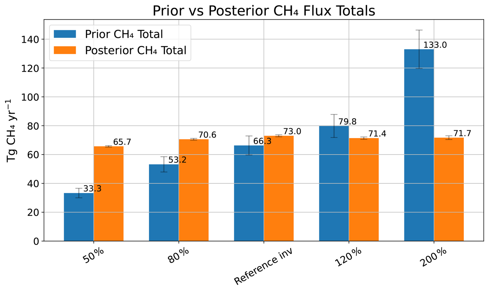
Figure 13 Sensitivity of total posterior methane emissions to prior flux magnitude scaling. The prior inventory was uniformly scaled to 50 %, 80 %, 120 %, and 200 % of its original magnitude. Blue bars show the corresponding prior totals and orange bars the posterior totals.

Despite large perturbations to the prior magnitude (ranging from 33 to 133 Tg CH₄ yr⁻¹), the posterior fluxes converge toward a relatively narrow range of approximately 65 to 73 Tg CH₄ yr⁻¹. This behavior indicates that the inversion is not strongly controlled by the absolute magnitude of the prior emissions and that the observational constraint plays a dominant role in determining the posterior total emissions.

The spatial increment patterns remain consistent across all the members, preserving the same regional structure of positive and negative adjustments relative to the prior. Overall, this sensitivity analysis suggests that the national-scale posterior estimates are relatively robust to large changes in prior flux magnitude.

3.4 Ensemble of Inversions

To quantify the sensitivity of our inversion to the uncertainty assumptions, we performed nine inversions combining three levels of prior flux uncertainty (50 %, 100 %, 200 %) with three background error settings (0.3 %, 0.5 %, 0.7 %). Posterior fluxes for South Asia range from 65.16 to 74.62 Tg yr⁻¹, with an ensemble mean of 70.97 Tg yr⁻¹, a standard deviation of 3.16 Tg yr⁻¹, and an ensemble spread of 9.46 Tg yr⁻¹ (∼ 13 % of the mean), illustrating the uncertainty introduced by our prior choices (Fig. 14). For the simulations with the lowest prior uncertainty (50 %) and the highest prior uncertainty (200 %), increasing the background error from 0.3 % to 0.7 % reduces the posterior fluxes, whereas for the simulations with the moderate prior uncertainty (100 %), posterior fluxes show a slight increase from 73.0 to 73.8 Tg yr⁻¹, but are remarkably stable (< 1 Tg yr⁻¹ change). This demonstrates a robust solution under moderate changes of a-priori background uncertainty.

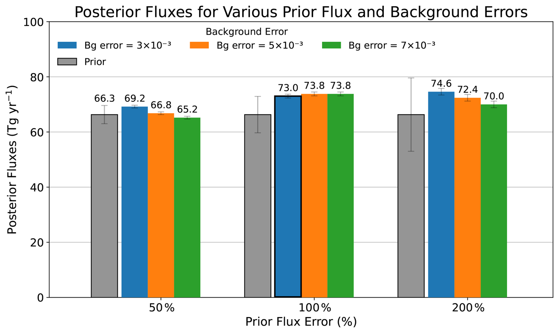
Figure 14 Posterior CH₄ flux estimates as a function of prior-flux uncertainty (50 %, 100 %, 200 %) and three background-error settings (0.3 % in blue, 0.5 % in orange, 0.7 % in green). The reference inversion is outlined in black. The prior flux and its uncertainty are shown as separate grey bars for each group for comparison.

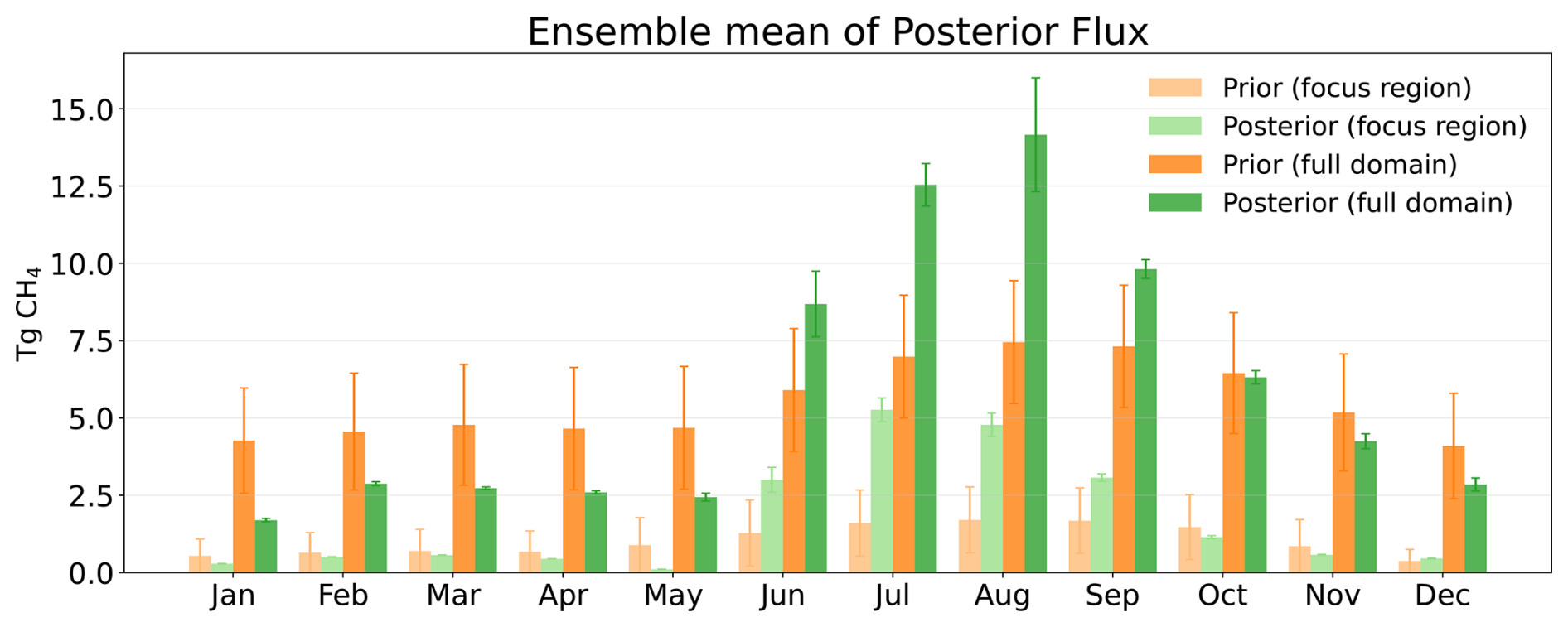
Figure 15 Ensemble mean monthly CH₄ fluxes (Tg yr⁻¹ CH₄), showing prior estimates (orange) and posterior means (green) with ±1σ error bars across nine inversion experiments. Error bars for the prior represent the prescribed prior uncertainty used in the reference inversion.

Figure 15 presents the monthly ensemble means of posterior fluxes compared with the priors, with the error bars (±1σ) indicating 1σ spread across the nine inversion experiments. The darker shaded bars correspond to the full South Asia domain, while lighter shades represent the Bangladesh focus region. Across all ensembles, the posterior fluxes exhibit a consistent and robust seasonal cycle. Posterior flux adjustments are negative during January to May and again in October to December. The ensemble spread remains very small during this period, when the number of TROPOMI observations is large (Fig. 2). In contrast, June to September shows strong positive increments, particularly in the Bangladesh focus region where posterior fluxes nearly triple the priors, reflecting the severe flooding and widespread soil inundation. The ensemble spread is largest during June to August, reaching ±2 Tg yr⁻¹ for the full domain and ±0.8 Tg yr⁻¹ for the focus region, coinciding with reduced satellite coverage under cloudy monsoon conditions. Importantly, the increments are not only consistent in time but also across space, with all ensemble members showing a coherent increase in emissions over the same regions. The persistence of these adjustments across all ensemble members highlights the robustness of the inversion in capturing the influence of the South Asian monsoon and hydrology on methane emissions.

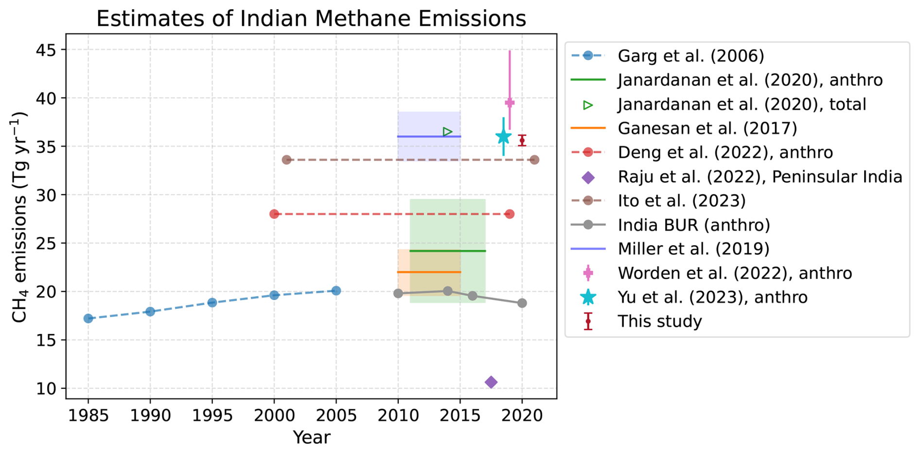
Figure 16 Comparison of methane (CH₄) emission estimates over India from previous studies. Multi-year means and associated uncertainties are shown, along with our 2020 estimate.

Figure 16 summarizes the estimates of methane emissions over India from various studies and provides our results in context. The estimates underscore significant heterogeneity across methodologies and observation periods. A clear separation can be seen between earlier bottom-up based estimates such as Garg et al. (2006) and India BUR reports and more recent satellite-constrained top-down studies (Janardanan et al., 2020; Worden et al., 2022; Yu et al., 2023), with the latter generally indicating higher emissions. These estimates reinforce the growing evidence that bottom-up inventories likely underestimate methane emissions over South Asia and highlights the value of satellite observations for constraining regional methane budgets, particularly in regions where ground-based in situ measurements remain extremely sparse.

4 Conclusion

This study demonstrates the value of assimilating TROPOMI satellite observations into a Bayesian inversion framework to constrain regional methane emissions over South Asia. The inversion substantially improves the agreement between observed and modeled mole fractions, as seen by the increase in correlation from 0.65 to 0.89 and the shift toward an unbiased fit. Posterior fluxes reveal substantial underestimations in the inventories over wetland-rich and intensively cultivated regions like eastern India and Bangladesh as well as in the Indus river basin. The inversion estimates a total of 73.0 Tg yr⁻¹ CH₄ emissions for South Asia in 2020, which is 6.7 Tg yr⁻¹ higher than the prior estimate. Within this increase, Bangladesh alone contributes +5.6 Tg yr⁻¹, while the region covering eastern India and Bangladesh (black box) accounts for +8.4 Tg yr⁻¹ of the regional increment. In contrast, western India and northern Pakistan show negative adjustments, suggesting overestimation of fluxes in the prior inventories. However, a localized region within the Lower Indus Basin shows a notable positive increment (∼ 0.5 Tg yr⁻¹), with the posterior fluxes capturing a distinct dual-peak seasonality (May and August) absent in the prior estimates. This enhanced seasonality coincides with the runoff cycle of the Indus River, which is modulated by both glacier and snowmelt from the Upper Indus and by monsoonal rainfall and irrigation in the lower basin.

Importantly, the prior emissions overestimate methane during the early part of the year (January–May, by 46 %) as well as during November–December (by 13 %), while underestimating it during June–September (by 70 %) – a seasonal mismatch corrected by the inversion. Most of the spatial and temporal corrections coincide with the regions of heavy monsoonal rainfall. Further analysis shows increased correlation between posterior fluxes and key environmental drivers like precipitation, soil moisture, and runoff. These analyses suggest that the rise in methane emissions is very likely linked to biogenic processes driven by glacial melt (in the Indus river basin), heavy monsoonal rainfall and enhanced inundation (both in the Indus river basin and in Bangladesh). These findings are consistent with earlier studies (e.g., Ganesan et al., 2017; Janardanan et al., 2020; Peng et al., 2022; Niwa et al., 2025) that identify wetlands and agriculture as dominant contributors to the regional and global methane budget in recent years. At the same time, it is important to note that the anomalous global methane growth in 2020 has also been partly attributed to a reduction in atmospheric OH concentrations during COVID-19 lockdowns (Ciais et al., 2026). However, inventories do not reproduce the important seasonal variability of emissions in the large river systems – a finding that may apply also to other regions than South Asia. It should also be emphasized that the present analysis reflects a single-year inversion for 2020 and extending the analysis to multiple years would enable robust quantification of interannual variability and flux–hydrology relationships and represents an important direction for future work.

A nine-member ensemble of inversions provides a robust sensitivity analysis, quantifying the spread introduced by varying prior flux and background mole fraction errors. The posterior emissions vary within a ∼ 9.5 Tg yr⁻¹ range, with the most stable results achieved under moderate a priori uncertainty (100 %). Seasonal patterns in all posterior ensembles show enhanced emissions during the monsoon months. The spread across ensemble members was low during the dry months, indicating robust agreement when observational coverage was sufficient. In addition, sensitivity tests in which the prior flux magnitude was scaled between 50 % and 200 % of the reference inventory show that posterior total emissions converge toward a relatively narrow range (∼ 65–73 Tg yr⁻¹), with consistent spatial increment patterns across experiments, indicating that the inversion results are not strongly controlled by the assumed prior magnitude. The ensemble results highlight the critical role of prior uncertainty settings in inverse modeling and demonstrate the necessity of ensemble approaches for deriving robust uncertainty estimates. However, the analysis is based on the TROPOMI WFMD retrieval product, and a systematic assessment of retrieval-dependent differences (e.g., using the operational TROPOMI retrieval product) remains an important avenue for future work. Overall, this work provides a refined top-down constraint on South Asia's methane emissions for the year 2020 and highlights key spatial and seasonal discrepancies in existing inventories, offering guidance for future improvements in emission reporting and process-based modeling.