The remarkable inefficiency of stratocumulus

Marine stratocumulus clouds play a central role in Earth's climate system by reflecting incoming solar radiation and exerting a strong cooling effect. Their organization into open and closed mesoscale cellular morphologies can be thought of as an example of bistable dynamics driven by aerosol–cloud interactions and mesoscale processes. From the perspective of non-equilibrium thermodynamics, these structures are an example of a far-from-equilibrium open system that continuously produces and exports entropy. While entropy production has been studied in idealized deep convective systems, it has not yet been quantified for shallow clouds. Here, we compute and decompose the internal entropy production of open- and closed-cell stratocumulus using an ensemble of large-eddy simulations. We show that the overall entropy production of stratocumulus is low, reflecting the limited vertical extent and corresponding reduced ability to utilize the energy fluxes at the system's boundaries. Moist processes dominate the overall irreversibility, which, combined with their low entropy production, leads to a mechanical efficiency about an order of magnitude smaller than in deep convective systems. Although the dominant irreversible processes differ between open- and closed-cell regimes, the distributions of total entropy production largely overlap across the ensemble, limiting the ability to distinguish the dynamics of individual cases based solely on total entropy production.

1 Introduction

Covering roughly a quarter of the oceans, marine stratocumulus clouds are the most common cloud type by area and exert a strong cooling effect by efficiently reflecting incoming solar radiation (Hahn and Warren, 2007; Stephens and Greenwald, 1991). Stratocumulus often self-organize into striking mesoscale cellular patterns in two distinct configurations. Closed cells have cloudy interiors and narrow, cloud-free edges. They are primarily driven by cloud-top radiative cooling and are generally associated with minimal precipitation, representing a top-down driven convective regime (e.g. Lilly, 1968; Schubert et al., 1979). In contrast, open cells appear as the inverse pattern, with cloud-free interiors surrounded by cloudy edges. These are maintained by cold-pool dynamics and feature light localized drizzle (Savic-Jovcic and Stevens, 2008; Wang and Feingold, 2009; Koren and Feingold, 2013; Xue et al., 2008). It has been hypothesized that these morphologies may represent two dynamically stable states of mesoscale organization within the coupled aerosol-cloud-precipitation system, mostly distinguished by their low (open cells) or high (closed cells) cloud droplet number concentration (Bretherton et al., 2010; Koren and Feingold, 2011; Glassmeier et al., 2021).

Since the cloud fraction and scene albedo of open and closed cells are so different, Earth's energy budget is highly sensitive to the balance between these different morphologies within the climate system. Understanding how and why stratocumulus clouds self-organize is therefore crucial to reducing uncertainties in climate sensitivity and magnitude of transient warming of the climate in the 21st century (Bony and Dufresne, 2005; Myers et al., 2021; Ceppi et al., 2024).

Unfortunately, stratocumulus remain notoriously difficult to model. Their shallow vertical extent and sharp inversions demand very high vertical resolution (Stevens and Bretherton, 1999), while their cold-pool dynamics are highly sensitive to horizontal grid spacing (Hirt et al., 2020; Fiévet et al., 2023). Furthermore, their apparent bistable dynamics are caused by processes operating on a wide range of scales, from collision-coalescence efficiencies at the microphysical level (Baker and Charlson, 1990) to cloud-top cooling and entrainment at the single cloud and mesoscale level (Hoffmann et al., 2024). Despite these challenges, Large Eddy Simulations (LES) have proven increasingly capable of reproducing the key features of stratocumulus regimes, including their mesoscale cellular organization and temporal evolution (Stevens et al., 2005; Feingold et al., 2015; Hoffmann and Feingold, 2019).

From a statistical physics perspective, the marine stratocumulus-topped boundary layer represents a non-equilibrium open system, with continuous exchanges of mass and energy at its boundaries. At the surface, latent heat is exchanged through evaporation and precipitation, while sensible heat is transferred by turbulent mixing. Above the inversion layer, subsidence and entrainment drive substantial energy and mass fluxes, and strong radiative cooling dominates energy loss (Wood, 2012; Hoffmann et al., 2020).

A defining feature of non-equilibrium systems is their continuous production of entropy sustained by continuous energy exchange with the environment. In the marine stratocumulus-topped boundary layer, high-quality energy enters at the ocean surface and exits at the colder cloud top as degraded energy. This thermodynamic quality gap, induced by differences in absolute temperature, drives the system's entropy dissipation, which in turn enables self-organization (Prigogine, 1968; Gaspard, 2022). Studying how entropy is produced and exported can provide a way to understand the emergent complexity and dynamical organization of the system.

Entropy production was first examined at the scale of the climate system as a whole (Paltridge, 1975; Stephens and O'Brien, 1993; Lucarini et al., 2010; Laliberté et al., 2015; Gibbins and Haigh, 2020; Kato and Rose, 2020). In the early 2000s, Pauluis and Held analyzed convective systems using idealized Radiative-Convective Equilibrium (RCE) simulations, decomposing the entropy budget into its components and linking them to physically meaningful processes such as updraft strength and convective activity (Pauluis and Held, 2002a, b). They showed how, for moist convection, most of the irreversibility is attributed to processes involving water (such as diffusion of water vapor, irreversible phase-changes and drag on hydrometeors) rather than turbulent dissipation. Subsequent studies have expanded this framework, applying it to both idealized RCE (Romps, 2008; Singh and O'Gorman, 2016; Singh and O'Neill, 2022) and to extreme events such as tropical cyclones (Ozawa and Shimokawa, 2015; Pauluis and Zhang, 2017; Fang et al., 2017; Régibeau-Rockett et al., 2023).

In this study, we quantify and analyze the entropy production in stratocumulus clouds, focusing on the closed and open cell morphologies. Using an ensemble of LES that resolve the bistable nature of stratocumulus, we examine not only the total magnitude of entropy production but also its decomposition into physically meaningful contributions. This framework allows us to examine how entropy production differs between open and closed cells, whether the dominant processes contributing to it change across regimes, and whether these differences help explain the system's tendency to organize into one state or the other. We also examine the thermodynamic constraints on stratocumulus clouds relative to deeper convective systems studied in RCE, focusing on their efficiency in driving atmospheric convection.

2 Mathematical formulation

For an open system, such as the atmospheric boundary layer, it is possible to express the total entropy S_tot tendency as (de Groot and Mazur, 2013)

$$\begin{array}{}\text{(1)}& {\displaystyle }{\displaystyle \frac{\mathrm{d}{S}_{\text{tot}}}{\mathrm{d}t}}={\displaystyle \frac{\mathrm{d}{S}_{\mathrm{i}}}{\mathrm{d}t}}+{\displaystyle \frac{\mathrm{d}{S}_{\mathrm{e}}}{\mathrm{d}t}}\end{array}$$

where S_i and S_e represent, respectively, the entropy produced inside the system and exported at the boundary. Here and in the following, S denotes the entropy (J K⁻¹), while s represents the specific entropy ($\mathrm{J}{\mathrm{K}}^{-\mathrm{1}}{\mathrm{kg}}^{-\mathrm{1}}$).

The second law of thermodynamics for an open system may be applied to the internal production, and reads

$$\begin{array}{}\text{(2)}& {\displaystyle }{\displaystyle \frac{\mathrm{d}{S}_{\mathrm{i}}}{\mathrm{d}t}}\ge \mathrm{0}.\end{array}$$

Equation (1) is the most general formulation of an entropy budget. The challenge is now to dissect all the components related to each term, in order to understand how the system distributes dissipation between different processes. For our analysis, we choose to adopt the material system view, which considers radiation simply as a reversible external source of heat, meaning that the entropic contribution from the interaction between photons and matter will not be taken into account. Not including radiation in the internal production allows one to focus on the water cycle and fluid dynamical processes (Singh and O'Neill, 2022). In particular, this translates into considering radiative cooling simply as an external heat sink for the system.

For a mixture of ideal gases heated reversibly by radiation, we may write a local entropy budget for the fluid as (Singh and O'Neill, 2022),

$$\begin{array}{ll}{\displaystyle }& {\displaystyle \frac{\partial \mathit{\rho }s}{\partial t}}+\mathbf{\nabla }\cdot \left(\mathit{\rho }\mathit{v}s\right)+\mathbf{\nabla }\cdot \left({\displaystyle \frac{{\mathit{D}}_{\mathit{u}}}{T}}+\sum _x{\mathit{D}}_{\mathit{x}}{s}_x\right)\\ \text{(3)}& {\displaystyle }& {\displaystyle }-{\displaystyle \frac{\mathit{\rho }{\dot{q}}_{\text{rad}}}{T}}=\mathit{\rho }{\dot{s}}_{\mathrm{i}}^{\text{mat}},\end{array}$$

where ${\dot{s_{\mathrm{i}}}}^{\text{mat}}$ represents the internal specific production of entropy. This equation contains bulk fluid quantities, such as the density ρ, the entropy density s, the fluid velocity vector v, its temperature T, and the radiative heating rate ${\dot{q}}_{\text{rad}}$. We then have the diffusive fluxes of sensible heat D_u and of species D_x, each carrying its entropy density s_x (Hauf and Höller, 1987). Here x represents dry air, water vapor and liquid water.

To study the total entropy production in the system, we integrate Eq. (3) over the system's volume Ω, defined as the atmospheric layer from the ocean surface up to just above the inversion. Formally, the balance between total internal production and external export can be then written as

$$\begin{array}{}\text{(4)}& {\displaystyle }{\displaystyle }\underset{\mathrm{\Omega }}{\int }{\displaystyle \frac{\partial \mathit{\rho }s}{\partial t}}+\underset{\mathrm{\Omega }}{\int }\mathit{\rho }\dot{s}{|}_{\text{subs}}+\underset{\partial \mathrm{\Omega }}{\int }{F}_{\text{ext}}+\underset{\mathrm{\Omega }}{\int }{\displaystyle \frac{\mathit{\rho }{\dot{q}}_{\text{rad}}}{T}}=\underset{\mathrm{\Omega }}{\int }\mathit{\rho }{\dot{s}}_{\mathrm{i}}^{\text{mat}}.\end{array}$$

On the left-hand side are the total tendency together with the entropy fluxes into the system F_ext. These fluxes include that owing to large-scale subsidence, the surface sensible heat flux, and mass fluxes associated with evaporation and precipitation. Subsidence is implemented in the model as a direct tendency on temperature and humidity that together gives a tendency of entropy ${\dot{s}}_{\text{subs}}$, which we integrate over the domain. The divergence in Eq. (3) gives rise to the surface fluxes of sensible heat, evaporation and precipitation, entering the domain at the surface temperature. Unlike in RCE (Pauluis and Held, 2002a; Singh and O'Neill, 2022), surface evaporation and precipitation are not in balance, meaning that the mass fluxes cannot be expressed simply in terms of the latent heat flux. Radiative cooling is incorporated by the last term on the left-hand side. While often considered as an external flux, entrainment across the inversion is treated here as an internal process since its effects, turbulent mixing and drying, occur within the system's volume.

In our stratocumulus simulations the storage term has a substantial contribution and cannot be ignored. This also complicates the interpretation of the external fluxes, particularly because individual terms depend on the chosen reference point for the entropy computation. Furthermore, given the small magnitude of the overall internal entropy production (Fig. 2), the external export, as written (left-hand side of Eq. 4), cannot be relied on to provide an estimate of the internal production. Our chosen LES model, the System for Atmospheric Modeling (SAM) (Khairoutdinov and Randall, 2003), has not been formulated to consistently treat entropy sources and sinks. For these reasons, we decided to focus directly on computing and studying the internal production, without trying to diagnose it via external fluxes.

To do so, we divide the internal specific production into the following components:

$$\begin{array}{}\text{(5)}& {\displaystyle }{\displaystyle }{\dot{s_{\mathrm{i}}}}^{\text{mat}}={\dot{s_{\mathrm{i}}}}^{\text{fric}}+{\dot{s_{\mathrm{i}}}}^{\text{heat}}+{\dot{s_{\mathrm{i}}}}^{\text{chem}}+{\dot{s_{\mathrm{i}}}}^{\text{mix}}+{\dot{s_{\mathrm{i}}}}^{\text{sed}}.\end{array}$$

The first two terms represent entropy production associated with the fluid mixture as a whole,

$$\begin{array}{}\text{(6)}& {\displaystyle }& {\displaystyle }\mathit{\rho }{\dot{s}}_{\mathrm{i}}^{\text{fric}}={\displaystyle \frac{\mathit{\rho }\mathit{ϵ}}{T}},\text{(7)}& {\displaystyle }& {\displaystyle }\mathit{\rho }{\dot{s}}_{\mathrm{i}}^{\text{heat}}=-{\displaystyle \frac{{\mathit{D}}_{\mathit{u}}\mathbf{\nabla }T}{T^{\mathrm{2}}}},\end{array}$$

where ϵ is the frictional dissipation due to viscosity at the end of the turbulent cascade, while ${\dot{s_{\mathrm{i}}}}^{\text{heat}}$ represents irreversibility associated with the diffusion of sensible heat. We then have the terms that are due to the active components in the mixture,

$$\begin{array}{}\text{(8)}& {\displaystyle }& {\displaystyle }\mathit{\rho }{\dot{s}}_{\mathrm{i}}^{\text{chem}}=-e{R}_{\mathrm{v}}\ln \left(R\right),\text{(9)}& {\displaystyle }& {\displaystyle }\mathit{\rho }{\dot{s}}_{\mathrm{i}}^{\text{mix}}\approx -R_{\mathrm{v}}{\mathit{D}}_{\mathrm{v}}\mathbf{\nabla }\ln \left({\displaystyle \frac{p_{\mathrm{v}}}{p_{\mathrm{0}}}}\right),\text{(10)}& {\displaystyle }& {\displaystyle }\mathit{\rho }{\dot{s}}_{\mathrm{i}}^{\text{sed}}=-{\displaystyle \frac{q_p{v}_{\mathrm{t}}}{T}}{\displaystyle \frac{\partial p}{\partial z}}.\end{array}$$

The first term, ${\dot{s_{\mathrm{i}}}}^{\text{chem}}$, corresponds to the contribution from non-equilibrium phase changes, where e is the evaporation rate, R_v is the specific gas constant of water vapor, and R is the relative humidity. Since there is no solid condensate in our domain, we do not account for contributions from phase changes involving solid water. The irreversible diffusion of substances in the fluid is counted in the second term, ${\dot{s_{\mathrm{i}}}}^{\text{mix}}$, for which the diffusion of water vapor is the dominant term (Pauluis and Held, 2002b). Here, p_v represents the partial vapor pressure, while p₀ is the reference point used for the entropy computation. Following previous studies (Pauluis and Held, 2002a; Singh and O'Neill, 2022), we will refer to the sum of ${\dot{s_{\mathrm{i}}}}^{\text{chem}}$ and ${\dot{s_{\mathrm{i}}}}^{\text{mix}}$ collectively as the contribution from moist processes. Finally, ${\dot{s_{\mathrm{i}}}}^{\text{sed}}$ represents the frictional effects on falling hydrometeors (Pauluis et al., 2000), where with v_t we indicate their terminal velocity.

In the following work, we will focus on estimating the total averaged internal material entropy production

$$\begin{array}{}\text{(11)}& {\displaystyle }{\displaystyle }〈{\dot{S}}_{\mathrm{i}}^{\text{mat}}〉={\displaystyle \frac{\mathrm{1}}{A}}\underset{\mathrm{\Omega }}{\int }〈\mathit{\rho }{\dot{s}}_{\mathrm{i}}^{\text{mat}}〉\mathrm{d}V,\end{array}$$

where 〈.〉 represents the time-average over a period for which the system can be considered to be approximately steady, such that the results can be considered representative for the case under study. We express the entropy production per unit surface area by dividing by the domain area A.

3 Simulations

To compute all the components of the entropy production in Eq. (5), we build upon an existing ensemble of Large Eddy Simulations run with SAM (Khairoutdinov and Randall, 2003). The dataset, first presented in Glassmeier et al. (2019), consists of 191 nocturnal stratocumulus simulations designed to explore cloud variability under controlled environmental conditions. The nocturnal setup was chosen to avoid the complexity of diurnal cycle forcing, allowing the system to equilibrate into a simpler quasi-steady state.

Each simulation is conducted on a $\mathrm{48}\mathrm{km}\times \mathrm{48}\mathrm{km}\times \mathrm{2}\mathrm{km}$ domain with 200 m horizontal and 10 m vertical grid spacing. The model is run for a total duration of 12 h. Simulations use constant surface fluxes, and a large-scale subsidence profile derived from a constant large-scale divergence, representative of typical marine stratocumulus conditions. SAM is configured to prognose supersaturation and employs a bin-emulating two-moment microphysics scheme that tracks both mass and number concentrations of cloud and rain droplets (Wang and Feingold, 2009).

Initial conditions were generated using a maximin Latin hypercube design (Morris and Mitchell, 1995) in a six-dimensional parameter space: mixed layer values of liquid water potential temperature ($\mathrm{284}<{\mathit{\theta }}_{\mathrm{l}}\left(\mathrm{K}\right)<\mathrm{294}$), total water mixing ratio ($\mathrm{6.5}<q_{\mathrm{t}}\left(\mathrm{g}{\mathrm{kg}}^{-\mathrm{1}}\right)<\mathrm{10.5}$), and aerosol concentration ($\mathrm{30}<N_{\mathrm{a}}\left({\mathrm{cm}}^{-\mathrm{3}}\right)<\mathrm{500}$), as well as the initial mixed layer height ($\mathrm{500}<H_{\text{mix}}\left(\mathrm{m}\right)<\mathrm{1300}$) and inversion jumps in temperature and moisture ($\mathrm{6}<\mathrm{\Delta }{\mathit{\theta }}_{\mathrm{l}}\left(\mathrm{K}\right)<\mathrm{10}$, $-\mathrm{10}<\mathrm{\Delta }{q}_{\mathrm{t}}\left(\mathrm{g}{\mathrm{kg}}^{-\mathrm{1}}\right)<-\mathrm{6}$) (Glassmeier et al., 2019). Following Glassmeier et al. (2019), we exclude cases that fail to sustain clouds or that produce precipitation within the first hour, leaving 159 simulations. The former correspond to lifting condensation levels above the inversion, while early precipitation cases exhibit rapid, non-physical dissipation of the cloud layer immediately after the 2 h spin-up. To avoid integrating over the model's sponge layer (starting at 1600 m), we additionally exclude cases with boundary layer depth exceeding 1500 m. The final dataset thus comprises 155 simulations, with 131 closed-cell and 24 open-cell cases.

The original ensemble does not include all diagnostics required for an accurate computation of the entropy production. To address this, we extend two representative cases by one additional hour, saving all relevant fields (see Sect. 3.1) at 5 min intervals. The selected cases capture the two characteristic cellular morphologies: one dominated by open cellular convection, the other by closed cells. These simulations were chosen based on their relatively small tendencies in key domain-mean quantities, such as liquid water path and droplet number concentration, indicating quasi-steady conditions (see Fig. 1). Although the boundary layer continues to evolve slowly, with non-zero tendencies in inversion height, the system remains sufficiently steady to permit reliable budget diagnostics.

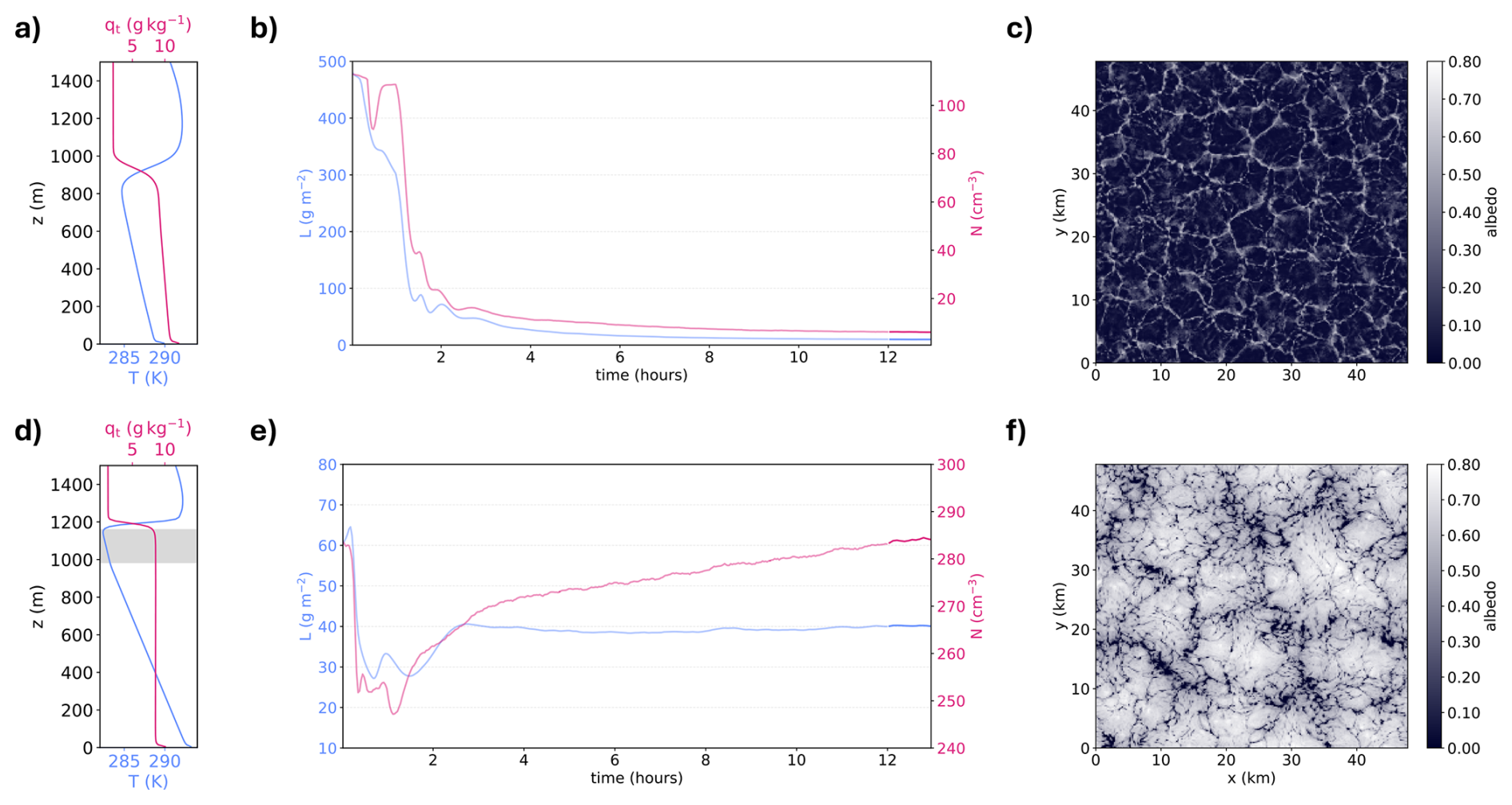
Figure 1 Detailed stratocumulus large-eddy simulations used for the entropy production analysis. (a–c) Open-cell and (d–f) closed-cell case with (a, d) 1 h time-averaged vertical temperature structure and total water mixing ratio q_t profile, (b, e) time series of domain-mean L (liquid water path) and N (droplet number concentration), and (c, f), snapshot of cloud albedo from the final timestep, highlighting the distinct morphology and fine-scale cellular patterns resolved by the LES. The cloud layer is indicated by the gray shaded region in panel (d), where it is well-defined in the homogeneous closed-cell case. In (b, e) light lines correspond to the original 12 h simulation, while solid lines indicate the 1 h equilibrated extension used for the entropy budget analysis.

3.1 Entropy budget computation for LES

All diagnostics are computed on the native LES grid using full 3D fields, prior to any spatial or temporal averaging. This is necessary because of the strong spatial variability of the boundary layer and the nonlinear nature of several terms in the entropy budget.

The viscous dissipation ϵ is taken directly from the subgrid-scale turbulent kinetic energy dissipation field, representing the local rate of conversion from mechanical energy to heat. Consistent with the LES formulation, diffusive fluxes are derived using the subgrid-scale eddy diffusivity and the model's 3D diffusion scheme. The condensation–evaporation rate e represents the net rate of phase change between water vapor and condensed water as diagnosed by the LES microphysics scheme. Finally, hydrometeor sedimentation is computed using terminal velocities from the LES microphysics scheme, diagnosed from droplet mean radius. With this approach, each term in Eq. (5) is computed consistently within the LES framework.

4 Moisture dominates the stratocumulus irreversibility

In Fig. 2 we present the decomposition of the internal entropy production for the two open- and closed-cell cases. Each entropy production term is integrated over the domain, averaged over the final hour and expressed per unit surface area of the model domain, following Eq. (11).

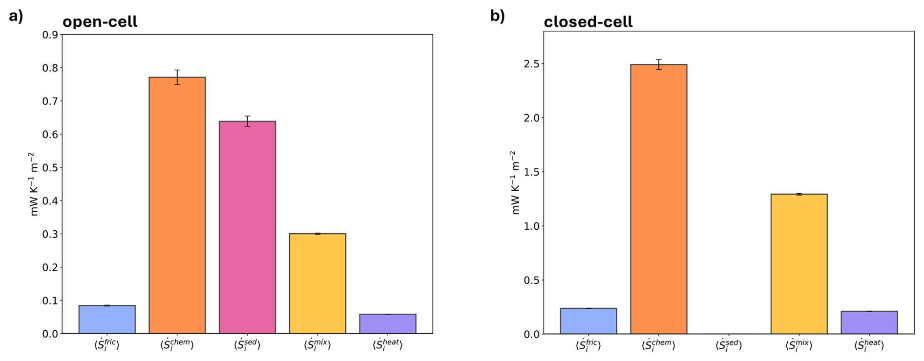
Figure 2 Internal entropy budget for (a) open-cell and (b) closed-cell stratocumulus. Variables on the x axis correspond to the terms in Eq. (5). Whiskers indicate one standard deviation over time. The budget is integrated over the full simulation domain up to z_max=1500 m and normalized by the domain surface area

We first note that the total entropy production differs markedly between the two morphologies: the closed-cell case produces more than twice as much dissipation as the open-cell case. This arises because the closed-cell simulation exhibits stronger rates of radiative cooling and subsidence drying at lower effective temperatures (Fig. A1), which increases entropy export and therefore requires higher internal production (Eq. 3).

While total entropy production is an indication of the degree of irreversibility generated, the specific decomposition of such dissipation is usually more informative for understanding the system's dynamics and self organization (Volk and Pauluis, 2010). We decompose the sources of entropy production following Eq. (5) and compare them with aggregated RCE results (Table 1). Consistent with earlier RCE findings by Pauluis and Held (2002b) and Singh and O'Neill (2022), we observe how moist processes dominate entropy production in stratocumulus clouds as well. We intentionally do not subdivide these contributions into diffusional and evaporation–condensation production, as the distinction is somewhat artificial and depends heavily on how the subgrid and microphysical processes are parameterized in the model. It can be shown that the entropy production due to the irreversible evaporation of liquid water at a relative humidity R is effectively the same as the production due to reversible evaporation at saturation followed by diffusion of water vapor down a vapor pressure gradient to the same value of relative humidity (Pauluis and Held, 2002b).

Table 1 Comparison of the (internal) entropy production due to different processes between open stratocumulus, closed stratocumulus, and aggregated RCE. Values for RCE are taken from Singh and O'Neill (2022). Open- and closed-cell results are averaged over the last hour of simulation.

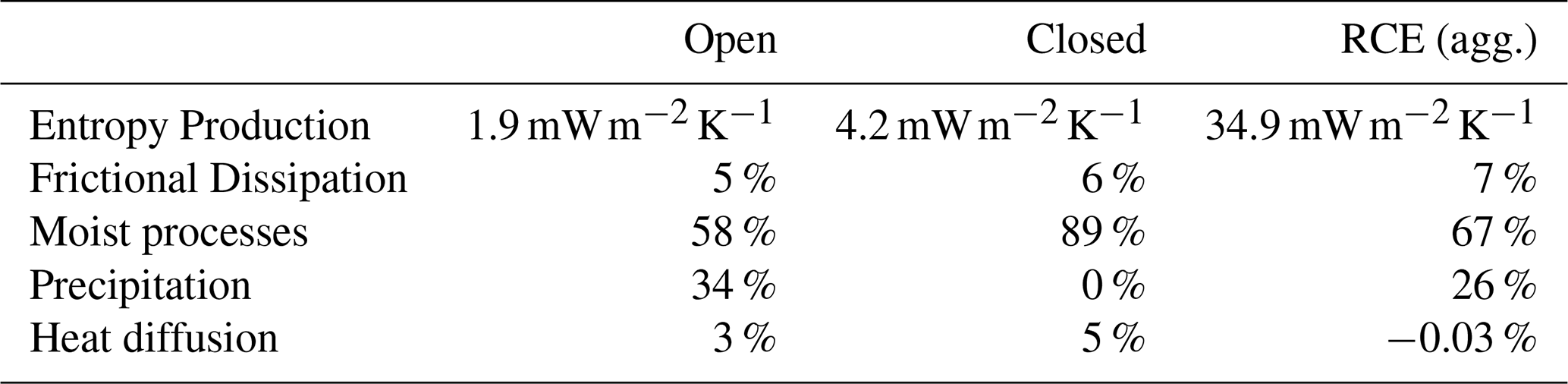
In the non-precipitating closed-cell case, moist processes account for approximately 90 % of the total entropy production, overwhelmingly outweighing frictional dissipation. This reflects the unique role of water vapor which, despite accounting for less than 1 % of the domain mass, is the only constituent able to undergo phase changes.

In the precipitating (open-cell) case, a substantial part of the dissipation appears to shift from moist processes to hydrometeor friction. Roughly one-third of total dissipation is attributed to precipitation drag, even more than in previous RCE simulations. At first glance, this result may seem counterintuitive, since frictional heating from falling hydrometeors is typically neglected in the energy budget of LES formulations such as SAM. This is often well justified, given that said frictional heating accounts for a minor source of heat, orders of magnitude less than radiative or surface fluxes (Igel and Igel, 2018). However, all of this heating is irreversibly dissipated, corresponding to a significant entropy source.

As a final contributor to internal entropy production, we find heat diffusion to be a non-negligible positive term. This contribution arises primarily from strong vertical gradients near the surface and at cloud top. While part of this diffusion is a model artifact due to the limited vertical resolution, we retain it for consistency with the model treatment. In contrast, previous RCE studies (Pauluis and Held, 2002a; Singh and O'Neill, 2022) found heat diffusion to be a minor term, and showing a negative sign. This apparent violation of the second law arises from how LES models handle subgrid-scale heat transport. As noted by Goody (2000), Romps (2008), Gassmann and Herzog (2015), parametrized turbulent heat fluxes do not always produce entropy in the same way as molecular diffusion. The second law is preserved by recognizing that turbulent heat transport and kinetic energy dissipation are part of the same cascade, so it is the total entropy production from all turbulent processes that must remain positive (Singh and O'Neill, 2022). However, given the strong differences in vertical resolution and model details between the two setups, we remark that a direct quantitative comparison of this term should be treated with caution.

Finally, we examine the relative contributions of horizontal and vertical components of the diffusion terms. Despite both closed and open cells exhibiting highly heterogeneous horizontal structures, both below and in cloud, nearly all of the entropy production from sensible heat and vapor diffusion (over 97 %) arises from vertical gradients (Fig. A2). We verified this result by rescaling to an isotropic grid, given the strong difference in horizontal and vertical grid spacing. While open cells show a stronger contribution from horizontal gradients in water vapor mixing, diffusion remains dominated by vertical gradients.

In terms of magnitude, the overall internal entropy production is low in both stratocumulus cases when compared to previous results in RCE simulations (Pauluis and Held, 2002a, b; Singh and O'Gorman, 2016; Singh and O'Neill, 2022). The comparison is presented in Table 1. We believe this discrepancy, exceeding one order of magnitude, can be attributed to the scale difference between systems. While the idealized RCE simulations typically involve deep convective clouds several kilometers deep (≈10 km), stratocumulus feature much shallower inversion heights, on the order of 1–2 km (Possner et al., 2020). Since entropy is an extensive quantity, it is unsurprising that deeper layers result in greater overall production. From an external perspective, a deeper layer translates to a bigger temperature difference across the layer (see Fig. A3), which allows for a larger difference between the input and output of entropy across the boundaries. An order of magnitude smaller vertical extent and temperature difference between stratocumulus and RCE translates to approximately an order of magnitude smaller total entropy production.

5 Moist production mirrors regime-specific processes

We now focus on moist processes, which represent the dominant contribution to the internal entropy production in both regimes. Not only does the share of moist production differ between the closed- and open-cell simulations, but the origin of this production also differs, directly reflecting the distinct physical drivers in each morphology.

In the closed-cell regime, moist entropy production is almost entirely driven by cloud-top entrainment, quantified by the entrainment velocity

$$\begin{array}{}\text{(12)}& {\displaystyle }{\displaystyle }w={\displaystyle \frac{\mathrm{d}{z}_{\text{inv}}}{\mathrm{d}t}}-w_{\text{subs}},\end{array}$$

estimated from the deepening of the boundary layer, where z_inv is the inversion height and w_subs the large-scale subsidence velocity. While some lateral mixing does occur, particularly at the boundaries between individual cells, the bulk of the moist production is strongly localized near the cloud top (Fig. A5). This is because closed-cell stratocumulus typically have intense vertical gradients in thermodynamic properties at the top of the boundary layer and relative horizontal homogeneity within the cloud deck (Wood, 2012). As a result, we find that the intensity of cloud-top entrainment scales with the total moist entropy production, as illustrated in Fig. 3. This highlights the fundamental role of cloud-top entrainment as a crucial driver of the organization and temporal evolution of closed stratocumulus decks (Wood, 2012; Kazil et al., 2017; Glassmeier et al., 2021).

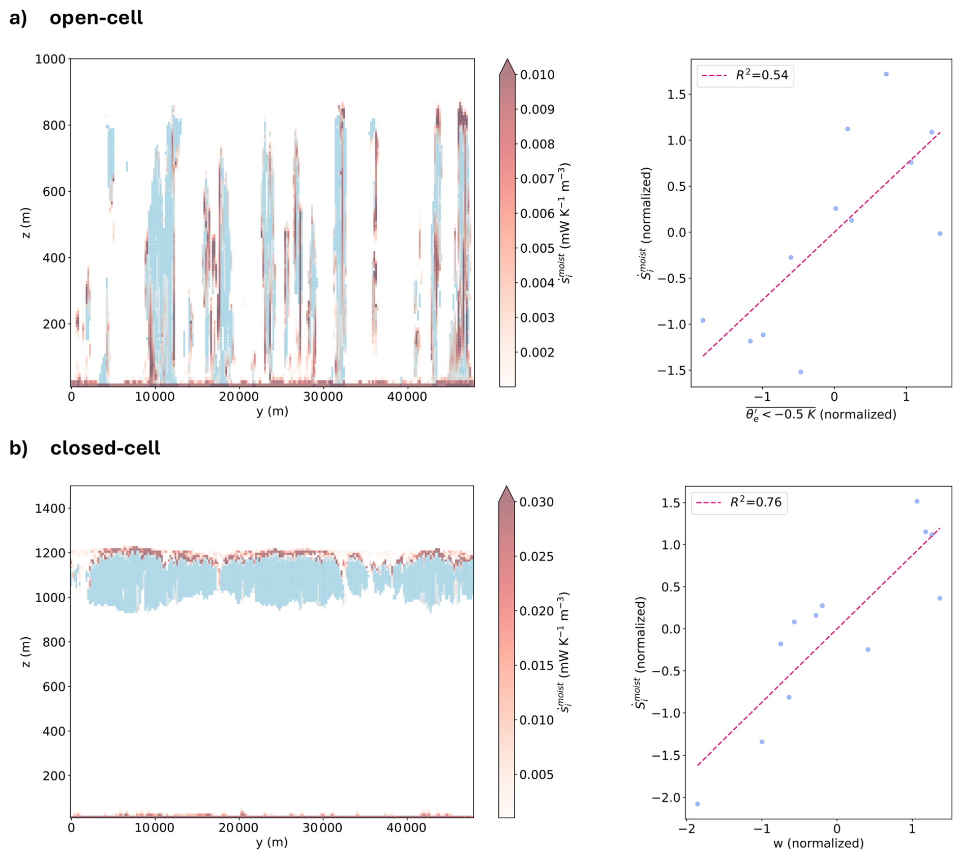
Figure 3 Regime dependencies of dominant moist processes. The left panels show a vertical cross-section of the moist entropy production at the last time-step. For open cells (row a), light shading highlights regions containing rain water, defined as locations where the rain water mixing ratio exceeds 0.01 g kg⁻¹. For closed cells (row b), shading indicates regions with cloud water mixing ratio above the same threshold. Only values of entropy production exceeding 0.001 $\mathrm{mW}{\mathrm{m}}^{-\mathrm{3}}{\mathrm{K}}^{-\mathrm{1}}$ are shown for clarity. The right panels show the correlation between the domain-mean moist entropy production ${\dot{S}}_{\mathrm{i}}^{\text{moist}}$ and the relevant thermodynamic variable: for open cells, the surface equivalent potential temperature anomaly conditioned on cold-pool regions ($\stackrel{\mathrm{‾}}{{\mathit{\theta }}_{\mathrm{e}}^{\prime }<-\mathrm{0.5}\mathrm{K}}$); for closed cells, the domain-mean entrainment velocity. Dashed lines indicate the linear regression, with the Pearson correlation coefficient reported in the legend.

In contrast, open-cell moist entropy production is governed by a completely different mechanism. Although cloud-top entrainment is still present, it plays a relatively minor role in the overall entropy budget. Similar to closed cells, a part of moist entropy production is localized near the surface due to strong vertical diffusion driven by surface fluxes. However, most of the entropy production originates from non-equilibrium phase changes in rainy columns (Fig. A4). In particular, rain evaporation is the dominant contributor, leading to the widespread formation of cold pools. These cold pools generate strong, sustained downdrafts near the centers of cells. When they collide with those from neighboring cells, they trigger new convective updrafts at cell boundaries, perpetuating the open-cell pattern (Wang and Feingold, 2009; Glassmeier and Feingold, 2017).

Because cold pools are driven by evaporative cooling, they are a direct dynamical manifestation of moist entropy production. This evaporative cooling represents thermodynamic entropy production associated with phase change in sub-saturated conditions. To quantify cold pool activity, we use the surface equivalent potential temperature anomaly (Alinaghi et al., 2025), ${\mathit{\theta }}_{\mathrm{e}}^{\prime }$, conditioned on cold pool regions defined by ${\mathit{\theta }}_{\mathrm{e}}^{\prime }<-\mathrm{0.5}\mathrm{K}$. The domain-mean value of this conditioned anomaly serves as our cold pool strength metric. As with closed cells, a significant relationship emerges between total moist entropy production and cold pool activity in the open-cell regime (see Fig. 3).

6 The remarkable inefficiency of stratocumulus

The stratocumulus-topped boundary layer is, as discussed earlier, shallow, with clouds that are an order of magnitude thinner than those in deep convective systems. This limited vertical extent translates directly into an order-of-magnitude smaller entropy production. Despite their shallow vertical extent, stratocumulus layers still exchange substantial energy across their boundaries, on the order of ∼100 Wm⁻² (Stevens et al., 2005; Kalmus et al., 2014; Glassmeier et al., 2019). To balance these inputs, the system releases energy primarily through strong radiative cooling, reaching values of ∼100 Kd⁻¹ in the dense closed-cell state. Interestingly, boundary fluxes of a similar magnitude are found in idealized RCE setups, despite the large difference in vertical scale (Pauluis and Held, 2002a; Singh and O'Neill, 2022). Why is stratocumulus convection then so weak compared to the vigorous updrafts in RCE?

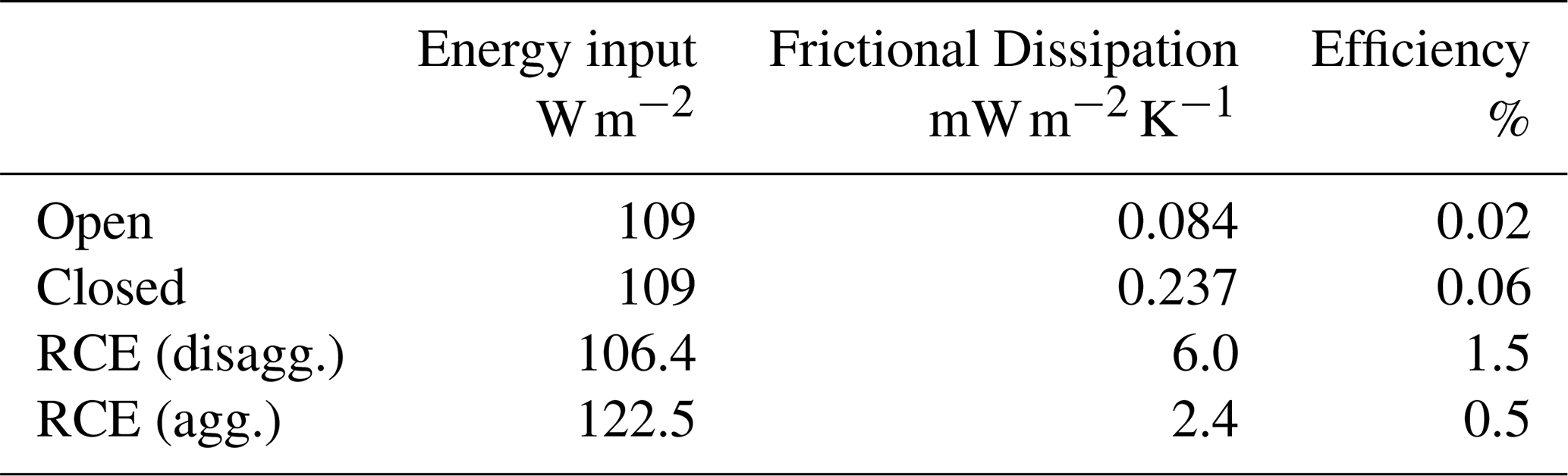
A useful lens is the mechanical efficiency of the system. Classically, efficiency describes how effectively a heat engine converts heat input into useful work. By analogy, the atmosphere can also be viewed as a heat engine, though with an important caveat: unlike a conventional engine, the atmosphere does not perform work on an external body. Instead, we can think of its useful work as the generation of kinetic energy through wind motions, ${\dot{W}}_{\mathrm{K}}$, which is ultimately dissipated internally via turbulence and friction (Rennó and Ingersoll, 1996; Lucarini, 2009). Following earlier work (Pauluis and Held, 2002a; Singh and O'Neill, 2022), we define the mechanical efficiency of the atmosphere as

$$\begin{array}{}\text{(13)}& {\displaystyle }{\displaystyle }\mathit{\eta }={\displaystyle \frac{\langle {\dot{W}}_{\mathrm{K}}\rangle }{|\langle {\dot{Q}}_{\text{in}}\rangle |}},\end{array}$$

where ${\dot{Q}}_{\text{in}}$ is the rate of energy input and angle brackets denote time averaging. In steady state, ${\dot{W}}_{\mathrm{K}}$ can be approximated with the turbulent dissipation rate (Pauluis and Held, 2002a), which includes the contribution from surface friction. For ${\dot{Q}}_{\text{in}}$, previous studies use the vertically integrated radiative cooling, which naturally balances the surface fluxes. In stratocumulus, however, subsidence warming and drying contribute substantially to the energy balance. This makes the choice of ${\dot{Q}}_{\text{in}}$ less straightforward than in RCE, where radiative cooling cleanly balances the surface fluxes and therefore provides an unambiguous measure of the heat input. In our simulations, radiative cooling and large-scale subsidence jointly act as a net energy sink for the boundary layer, while the only imposed energy input at the lower, warmer boundary is the prescribed surface sensible (F_sh) and latent (F_lh) heat fluxes (Fig. A6). We therefore define

$$\begin{array}{}\text{(14)}& {\displaystyle }{\displaystyle }{\dot{Q}}_{\text{in}}=F_{\text{sh}}+F_{\text{lh}}.\end{array}$$

This choice also reflects the fixed-flux boundary condition of our ensemble of simulations.

The resulting efficiencies for the open- and closed-cell simulations (Table 2) are low compared with typical RCE values (Pauluis and Held, 2002a; Singh and O'Neill, 2022). The higher turbulent kinetic energy dissipation in closed cells, relative to open cells, appears to result from their stronger cloud-top entrainment (see Appendix A). There are two competing effects that reduce the efficiency of stratocumulus convection. First, the maximum theoretical work available to the system is strongly constrained. The shallow vertical extent of the system severely limits the available temperature gradient, which in turn constrains the maximum work that could be generated from a given set of boundary fluxes and effective temperatures (Pauluis and Held, 2002a). Even if the system were to operate as an idealized heat engine, the small vertical scale alone strongly limits the amount of extractable work. The strong subsidence that characterizes stratocumulus regions acts as a mechanical lid, forcing the system to be confined to a shallow boundary layer with minimal temperature gradients (Wood, 2012). Furthermore, as argued by Pauluis (2011), the relative humidity at which the system operates also has an impact on the maximum amount of work, with drier systems being less efficient than moister ones. A thermodynamic cycle operating in a partially saturated environment has a maximum efficiency that increases with the degree of saturation, approaching the Carnot limit only in the fully saturated case. The departure from full saturation of the stratocumulus mixed layer therefore provides an additional constraint on the maximum extractable work.

Table 2 Summary of the energy input rate, frictional dissipation, and thermodynamic efficiency across different configurations. The RCE values for the disaggregated and aggregated states are taken from Singh and O'Neill (2022) and correspond to two regimes of the same simulation. In all cases, the energy input is defined as the sum of the surface sensible and latent heat fluxes. Reported values are averaged over the approximately steady periods selected for the analysis.

Second, only a fraction of this already limited maximum work is realized as kinetic energy. As in moist RCE, this is because moist processes dominate the dissipation budget. The presence of active moisture redirects much of the available energy into compensating irreversible phase changes, leaving relatively little to sustain atmospheric circulation.

Beyond the inefficient generation of kinetic energy, stratocumulus perform substantial work in lifting water within the domain against the large-scale subsidence, which we estimate as

$$\begin{array}{}\text{(15)}& {\displaystyle }{\displaystyle }\langle {\dot{W}}_q\rangle ={\displaystyle \frac{\mathrm{1}}{A}}\underset{\mathrm{\Omega }}{\int }\langle \mathit{\rho }gw{q}_{\mathrm{t}}\rangle \mathrm{d}V,\end{array}$$

where q_t is the total water mixing ratio and w the resolved vertical velocity. Time-averaged values for $\langle {\dot{W}}_q\rangle$ are 258 and 486 mW m⁻² for the open- and closed-cell cases respectively, largely exceeding $\langle {\dot{W}}_{\mathrm{K}}\rangle$ (24 and 68 mW m⁻²). In RCE, at steady-state this work is balanced by the dissipation of kinetic energy by falling hydrometeors within the domain (Pauluis and Held, 2002a). This balance does not hold in our simulations: open cells dissipate only approximately 183 mW m⁻² through precipitation, while the non-drizzling closed-cell case has negligible precipitation dissipation. In the real atmosphere, the water removed by subsidence would eventually precipitate in other regions, where the associated dissipation would occur. However, since this process does not happen inside our simulation domain, the associated dissipation is not accounted for in our entropy budget.

7 An ensemble perspective

The two detailed simulations analyzed so far provide a thorough understanding of how entropy is produced in each morphology. We now ask whether these behaviors are representative for the two states. Extending the budget analysis to the ensemble tests the robustness of our findings and highlights the systems' variability under transient behavior. Many simulations in the ensemble are not fully equilibrated, exhibiting non-negligible temporal tendencies in key variables (such as N, L, and z_inv), which can influence their entropy production. As mentioned earlier, the absence of full 3D fields limits our ability to compute all terms directly. Here we develop approximate formulas to estimate the entropy production using only horizontally averaged variables.

For the case of frictional dissipation and sedimentation, we find that simply replacing each variable in Eqs. (6) and (10) with their corresponding horizontally averaged values provides a very good estimate of the total entropy production. Water vapor diffusion is also reasonably well represented using horizontally averaged fluxes and fields. Heat diffusion in the closed-cell regime is less well captured, but given its low absolute contribution to the total entropy production, the resulting error does not significantly affect the overall budget. The dominant source of uncertainty is irreversible entropy production due to phase change.

To address this, we first separate the chemical term (Eq. 8) into its condensation and evaporation parts. Condensation occurs entirely at or slightly above saturation, resulting in evaporation being the dominant contribution. We then follow Singh and O'Gorman (2016) and construct an effective relative humidity profile weighted by the evaporation field,

$$\begin{array}{}\text{(16)}& {\displaystyle }{\displaystyle }{\stackrel{\mathrm{‾}}{\ln \left(R\right)}}_{\text{eff}}={\displaystyle \frac{{\int }_A\ln \left(R\right)E\mathrm{d}x\mathrm{d}y}{{\int }_{A}E\mathrm{d}x\mathrm{d}y}}={\displaystyle \frac{{\int }_A\ln \left(R\right)E\mathrm{d}x\mathrm{d}y}{\stackrel{\mathrm{‾}}{E}}},\end{array}$$

with E the 3D evaporation field. The overbar indicates that the quantity is a vertical profile, result of horizontal averaging. With this, we can write the full chemical entropy production term as

$$\begin{array}{ll}{\displaystyle }\underset{\mathrm{\Omega }}{\int }\mathit{\rho }{\dot{s}}_{\mathrm{i}}^{\text{chem}}& {\displaystyle }=-\underset{\mathrm{\Omega }}{\int }e{R}_{\mathrm{v}}\ln \left(R\right)\approx -\underset{\mathrm{\Omega }}{\int }E{R}_{\mathrm{v}}\ln \left(R\right)\\ \text{(17)}& {\displaystyle }& {\displaystyle }=-\underset{{\mathrm{\Omega }}_z}{\int }\overline{E}{R}_{\mathrm{v}}{\stackrel{\mathrm{‾}}{\ln \left(R\right)}}_{\text{eff}}\mathrm{d}z,\end{array}$$

which requires only vertical profiles to be computed. By doing this, we shift the burden of knowing the 3D fields of both evaporation and relative humidity to the requirement of obtaining the horizontally averaged profile of the effective relative humidity.

When evaporation stems mainly from precipitation, as is the case for RCE or stratocumulus open cells, the effective relative humidity field is only slightly higher than the horizontal mean (Singh and O'Gorman, 2016). For open-cell cases, we find that using Eq. (16) with the domain-mean $\stackrel{\mathrm{‾}}{R}$ provides a reasonable approximation of the condensation-evaporation contribution. In closed cells, however, all the moist production happens in the inversion layer, where sharp gradients make the relation between the effective relative humidity and the mean one non-trivial. We utilize the detailed closed-cell simulation to parameterize ${\stackrel{\mathrm{‾}}{\ln \left(R\right)}}_{\text{eff}}$, in order for it to be reconstructed using only the information available in all the simulations, i.e. vertical profiles.

Comparison of effective and mean profiles in the detailed run shows that the difference between them is confined to the entrainment layer, where the effective term remains higher well above cloud-top (see Fig. A7). This is due to the strong spatial correlation between the relative humidity and evaporation combined with the sharp inversion, which makes local spatial features stand out. Since the difference between the effective relative humidity and the spatial mean relative humidity is localized around the inversion, we parameterise this difference with a pulse-like function centered on the inversion. We find that the function's parameters can be easily tied to key physical quantities of the system, such as inversion height, cloud-top height, and inversion strength. For full details on the reconstruction, see Appendix B.

This approach allows a rough but practical parameterization of the effective field based on general boundary layer features and vertical profiles, which are available for all simulations in the ensemble. In this way, we can reconstruct the effective relative humidity profile, and therefore the moist production, using a minimal approach that allows us to take into account the variability between different ensemble members. Compared with directly using the mean vertical humidity profile, this procedure reduces the estimated moist entropy production by roughly 40 % (Fig. A7). While we cannot validate the procedure for all closed-cell runs, the behavior of the reconstructed moist production profiles across the ensemble matches what is observed in the detailed simulation (Fig. A8). This method provides a sufficient estimate of the domain-mean moist production, and a reasonable ensemble-averaged value, particularly given the large number (>100) of closed-cell cases available.

Applying this reconstruction procedure, we estimate the internal entropy production across the ensemble (Fig. 4, Table 3). As for the detailed cases, we find that, on average, closed-cell simulations exhibit a larger total production than open cells, driven by the strong cloud-top entrainment that dominates irreversibility in closed cells. The few open-cell outliers with unusually high values correspond to unsteady runs with strong negative tendencies in their entropy production. The detailed closed-cell case proves to be representative of the ensemble, while the detailed open-cell case lies at the lower end of the distribution. Both morphologies show considerable spread, reflecting the non-equilibrated nature of the simulations, and possible sensitivities to droplet number concentrations. Although liquid water path is nearly stabilized, droplet number concentration and inversion height still evolve substantially.

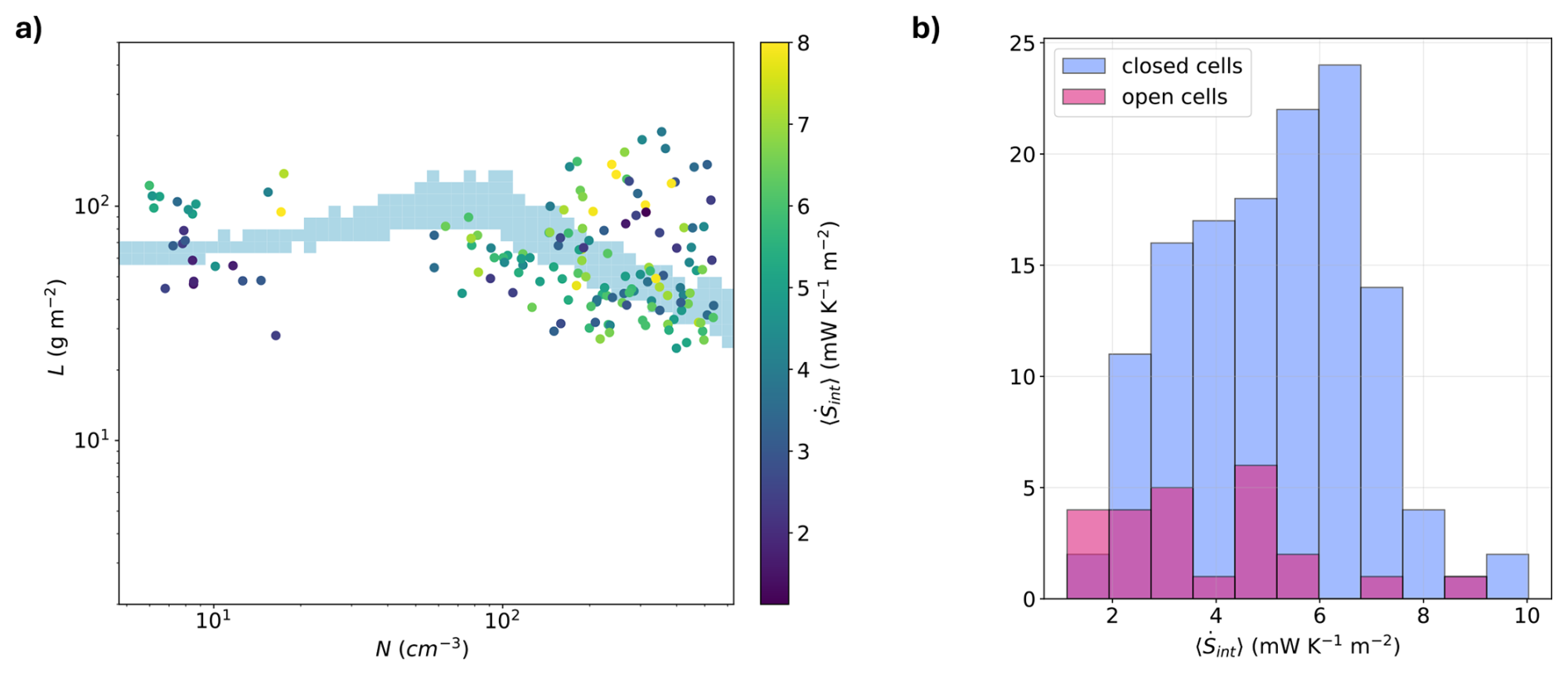
Figure 4 Ensemble projection of entropy production. Panel (a) shows the reconstruction of the total, time- and domain-averaged entropy production for the full LES ensemble, computed over the last hour of each simulation. Each point represents the domain-mean values of N (droplet number concentration) and L (liquid water path), averaged over that last hour, with the color indicating the corresponding total internal entropy production. The light blue shaded region in the background represents the L steady-state, extracted from the ensemble using Gaussian emulation (Glassmeier et al., 2021; Hoffmann et al., 2025; Chen et al., 2025). Panel (b) shows the distributions of the internal entropy production for the open- and closed-cell states, computed as in panel (a).

Table 3 Entropy production and efficiency approximation for the full LES ensemble. Values represent the median across the whole ensemble of simulations, computed from spatially averaged fields over the domain and temporally averaged over the final simulation hour. Values in brackets indicate the 25th–75th percentiles.

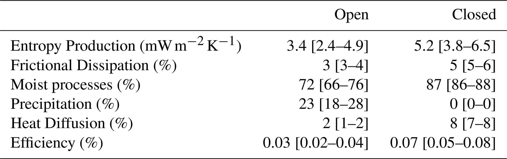
The term-by-term breakdown is summarized in Table 3. These ensemble results confirm the main findings from the detailed, single-case analyses: moist processes dominate the total dissipation, frictional dissipation remains small, and closed cells have a higher efficiency than open cells.

Furthermore, both morphologies show, on average, a higher share of entropy production attributable to moist processes compared to previous RCE results (Pauluis and Held, 2002a; Singh and O'Neill, 2022). This is consistent with previous work of Pauluis (2016), who extracted thermodynamic cycles of different depths from RCE convection and found that shallower cycles show a higher share of moist processes compared to deeper ones. Together with the results presented in this paper, this supports the relative importance of moist processes scaling inversely with the depth of the thermodynamic cycle.

8 Discussion and Conclusion

In this work we analyzed the internal entropy production of stratocumulus clouds, applying the entropy budget formalism that has so far been established for and applied to deep convection to both the open- and closed-cell morphologies. Our results reveal substantial differences in the partitioning of the entropy budget between the two states. As in earlier work on Radiative Convective Equilibrium (Pauluis and Held, 2002a, b; Singh and O'Gorman, 2016; Singh and O'Neill, 2022), moist processes dominate the total production in both regimes. We further identified how this dominant term reflects regime-specific processes: cloud-top entrainment in closed cells and cold-pool dynamics in open cells.

Unlike in RCE, stratocumulus exhibit an exceptionally small total dissipation. This limitation can be traced to their shallow vertical development, which constrains the available temperature gradient and thereby the maximum possible work. However, we note how, inside the stratocumulus regimes, the dissipation does not scale trivially with system size (e.g. inversion height), but instead depends on the specific organization of the cloud field and its properties (such as effective temperatures of energy exchange). This explains why stratocumulus convection remains mechanically weak, despite strong boundary fluxes, and why the system is characterized by such a low thermodynamic efficiency.

Recent work (Singh and O'Neill, 2022) suggests that convective organization itself modulates efficiency. In RCE, long integrations often exhibit self-aggregation (Bretherton et al., 2005; Emanuel et al., 2014), which reshapes the balance between frictional dissipation and moist processes. Stratocumulus, by contrast, represents a highly regular, space-filling form of organization (Glassmeier and Feingold, 2017). In closed-cell states, nearly the entire domain experiences cloud-top drying, with cloud fraction close to unity. This results from the absence of precipitation, which otherwise would break up cloud cover. Interestingly, while moist processes dominate the entropy budget far more strongly than in RCE, the lack of precipitation still leaves a relatively large share for kinetic dissipation, comparable to aggregated RCE (Singh and O'Neill, 2022). Open-cell organization, driven by precipitation, also shows a comparable fraction, only slightly lower than that in closed cells, relative to its total entropy production. This suggests that using the entropy budget to constrain dissipation can be difficult, since systems with vastly different dynamics and irreversible mechanisms can exhibit similar total frictional dissipation.

A key aspect of our analysis is the ensemble perspective. Mesoscale Stratocumulus boundary layers are never in steady-state. While liquid water path can relax on relatively short timescales (Schubert et al., 1979; Bretherton et al., 2010), droplet number concentration and inversion height often evolve on timescales comparable to those of the large-scale cloud controlling variables (Eastman et al., 2016). In such situations, a single simulation cannot be considered representative, since the system's trajectory strongly depends on its initial conditions. By utilizing a large ensemble, we are able to extract robust statistics. While the median total entropy production differs between the two morphologies, the considerable overlap between the two distributions suggests that entropy production alone is not sufficient to cleanly distinguish between open- and closed-cell convection.

The transient nature of our simulations, however, still poses some limitations. While the terms analyzed in this study can be considered steady on the timescale analyzed, the system still contains strong internal tendencies. This is the main reason why we chose to focus on the internal production directly, and did not try to diagnose it by means of the external export (see Eq. 4). While the external view can provide important insights into how the system exchanges energy and mass at its boundary, in our case it is of limited applicability.

Our results also provide insights into the relationship between multistability and entropy production. For non-equilibrium systems, much work has been devoted to characterizing how nature selects the fate of a system, especially when there may be multiple possible steady states. Theories exist for linear systems close to equilibrium (Onsager, 1931; Prigogine, 1968), but for systems far from equilibrium, there is currently no consensus on how and if the long-term evolution of the system can be predicted without explicit simulation of its temporal trajectory. One hypothesis is the maximum entropy production principle (Paltridge, 1975; Ozawa et al., 2003; Kleidon, 2004), which suggests that systems select states that maximize dissipation, though its validity remains debated. In multi-stable situations, it has been recently argued that nature selects the state that dissipates the most (Endres, 2017), with the principle formulated probabilistically, relating total dissipation to stability.

In our stratocumulus case, we find that, although the median internal entropy production differs between the open- and closed-cell states, their distributions largely overlap. A stochastic analysis of our LES ensemble shows that the probabilistic landscape is not symmetric, with the open-cell state being the more stable of the two (Hernandez and Glassmeier, 2026). Therefore, the total irreversible entropy production does not appear to select the observed state, and the open-cell configuration, contrary to a maximum entropy production expectation, instead has a lower median dissipation. Both stable states exhibit similar entropy production magnitudes but are governed by different feedbacks and dynamics.

Appendix A: Subgrid-scale turbulent kinetic energy budget

To understand differences in turbulent kinetic energy (TKE) dissipation between open and closed cells, we analyze the subgrid-scale (sgs) TKE budget, which can formally be written as

$$\begin{array}{}\text{(A1)}& {\displaystyle }{\displaystyle \frac{\partial e}{\partial t}}=P_{\mathrm{s}}+P_{\mathrm{b}}+T-\mathit{ϵ},\end{array}$$

where e is the sgs TKE. The right-hand side consists of shear production P_s, buoyancy production P_b, transport T, and sgs dissipation ϵ, which contributes to the frictional dissipation in Eq. (5). When spatially integrated over the domain, the transport term vanishes.

Figure A9 shows the integrated sgs budget for the two runs. We observe how, after a brief equilibration, dissipation is almost completely dominated by shear production,

$$\begin{array}{}\text{(A2)}& {\displaystyle }{\displaystyle }\underset{\mathrm{\Omega }}{\int }\mathit{ϵ}\mathrm{d}V\approx \underset{\mathrm{\Omega }}{\int }{P}_{\mathrm{s}}\mathrm{d}V.\end{array}$$

Shear production is notably higher in closed cells, primarily due to strong cloud-top entrainment characteristic of stratocumulus. As seen in Fig. A10, the largest contributions occur at the entrainment layer, where the sgs shear is strongest. These differences are robust across the ensemble, explaining why closed cells generally experience higher frictional dissipation and, consequently, a higher mechanical efficiency than open cells.

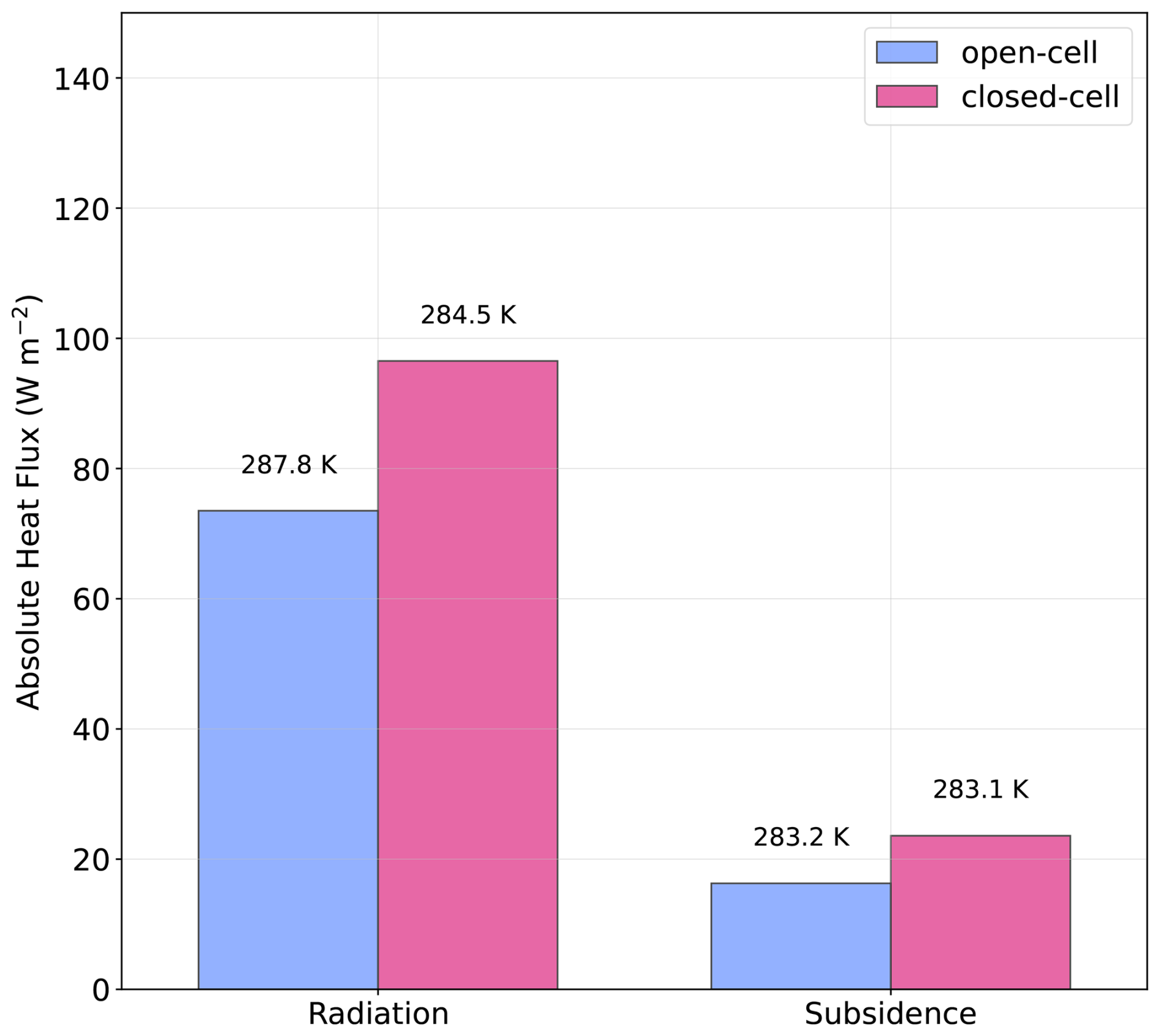
Figure A1 Energy export for the detailed open cell and closed cell runs. For both scenarios, both energy fluxes act as net sinks for the system. The temperatures reported are effective temperatures, computed by weighting the respective heating tendency over the whole domain, following Singh and O'Neill (2022). The values here reported have been averaged in time over the last simulation hour.

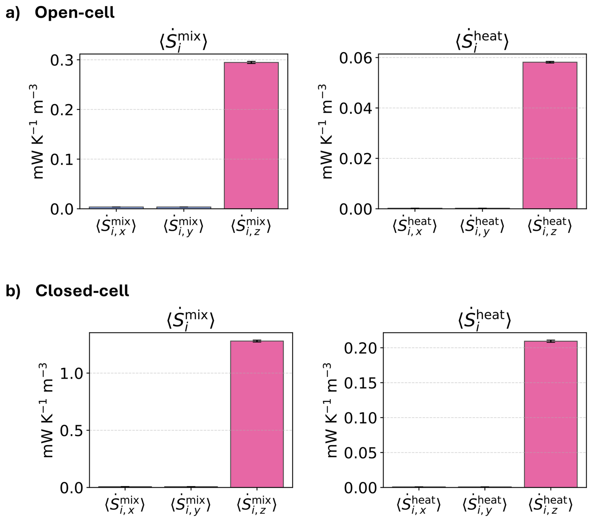
Figure A2 Comparison of horizontal and vertical diffusion contributions. Time-averaged horizontal and vertical contributions to the entropy production from diffusion of water vapor (Eq. 9) and sensible heat (Eq. 7) for the open- (a) and closed- (b) cell cases. The terms are integrated up to z_max=1500 m and normalized by the domain surface area. Values are averaged over the last simulation hour, with whiskers indicating ±1 standard deviation over time. Horizontal contributions account for approximately 2 % and 1 % of the total for water vapor mixing in the open- and closed-cell cases respectively, and less than 1 % for sensible heat in both cases.

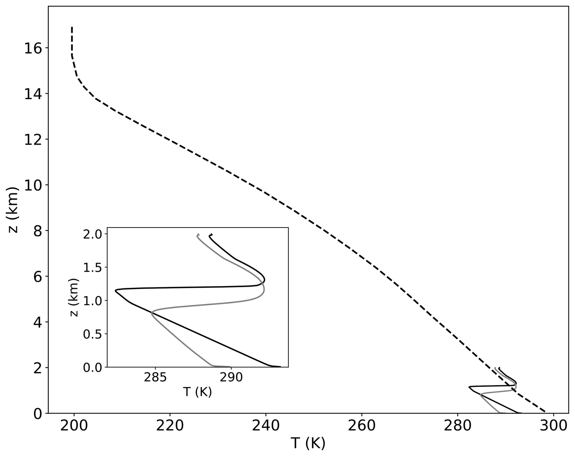
Figure A3 Comparison of system scales between RCE and stratocumulus clouds. The RCE temperature profile (dashed line) is taken from the moist RCE simulation in Singh and O'Neill (2022). For the stratocumulus cases, the darker line corresponds to the detailed closed-cell simulation, while the lighter line corresponds to the detailed open-cell simulation. The inset shows a zoomed-in view of the vertical temperature structure for the stratocumulus cases.

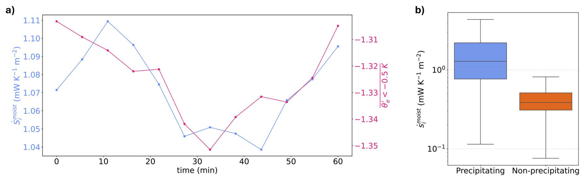
Figure A4 Moist production in open cells. Panel (a) shows the time series of domain-mean moist entropy production ${\dot{S}}_{\mathrm{i}}^{\text{moist}}$ and the surface equivalent potential temperature anomaly, conditioned on cold-pool regions ($\stackrel{\mathrm{‾}}{{\mathit{\theta }}_{\mathrm{e}}^{\prime }<-\mathrm{0.5}\mathrm{K}})$. Panel (b) shows the moist entropy production, separated into contributions from rainy (Precipitating) and non-rainy (Non-precipitating) columns, using a total rain water threshold of 1 g kg⁻¹.

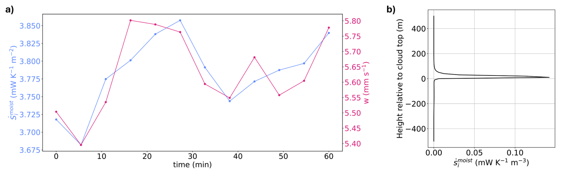
Figure A5 Moist production in closed cells. Panel (a) shows the time series of domain-mean moist entropy production ${\dot{S}}_{\mathrm{i}}^{\text{moist}}$ together with the domain-mean entrainment velocity. Panel (b) displays the horizontally averaged moist production profile, with each column rescaled and centered around the cloud-top height on the vertical axis.

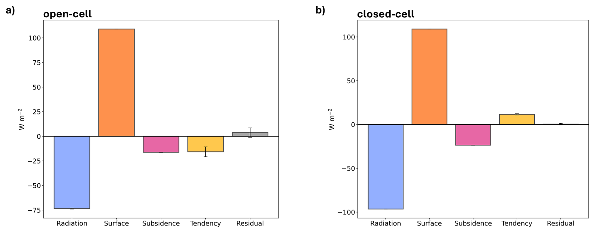
Figure A6 Energy balance for (a) open-cell and (b) closed-cell stratocumulus. The columns represent, respectively: radiative cooling, surface fluxes (F_sh+F_lh), subsidence, total tendency and residual. Whiskers indicate one standard deviation over time. The terms are integrated over the full simulation domain up to z_max=1500 m and normalized by the domain surface area. The values here reported have been averaged in time over the last simulation hour.

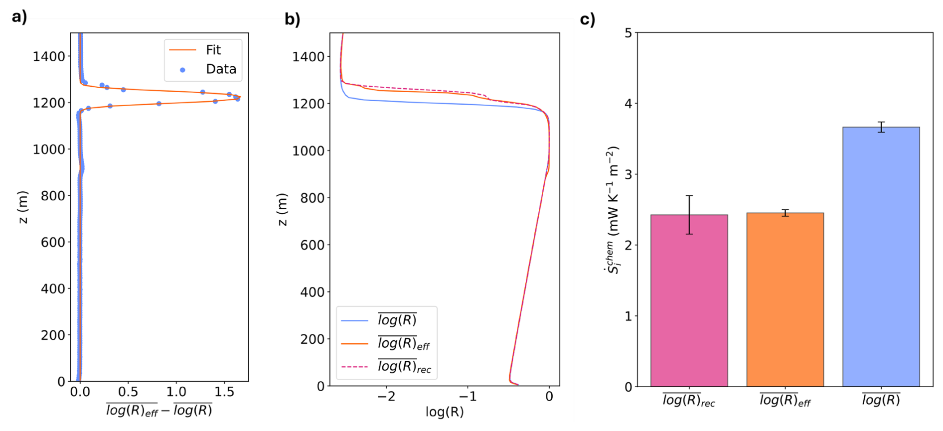
Figure A7 Reconstruction of effective relative humidity. Panel (a) shows the fit to the difference between the time averaged effective and actual relative humidity. Panel (b) shows the time averaged profiles of the actual, effective, and reconstructed relative humidity using Eq. (B2). Panel (c) shows the estimated entropy production from non-equilibrium phase changes when the effective humidity of evaporation is estimated using the full 3D data (${\stackrel{\mathrm{‾}}{\log \left(R\right)}}_{\text{eff}}$), the horizontal-mean relative humidity ($\stackrel{\mathrm{‾}}{\log \left(R\right)}$), and the reconstructed relative humidity based on Eq. (B1) (${\stackrel{\mathrm{‾}}{\log \left(R\right)}}_{\text{rec}}$). Whiskers show one standard deviation in time.

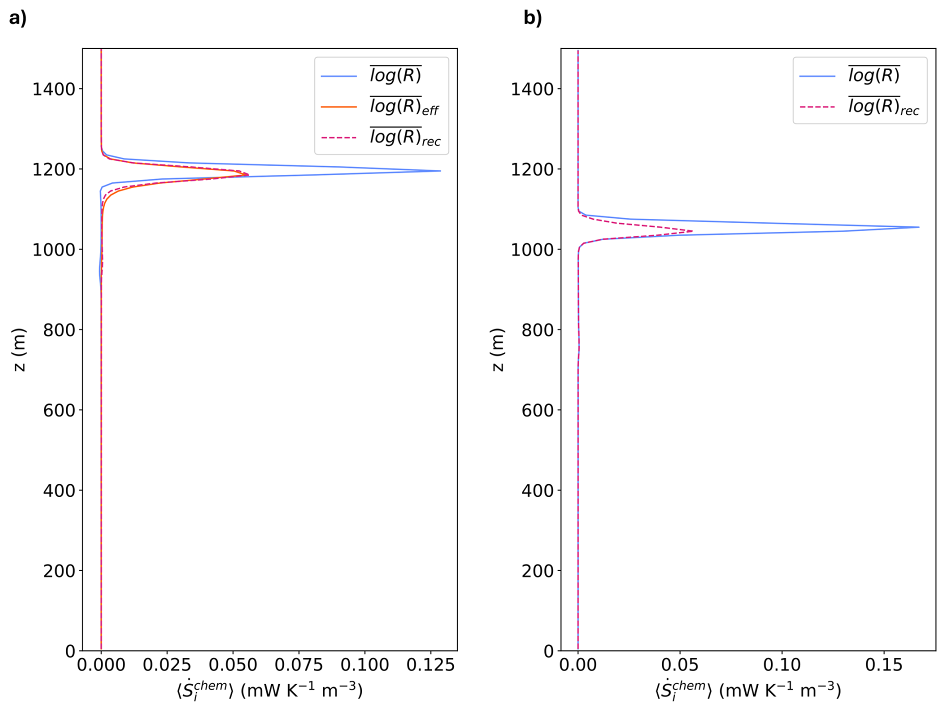
Figure A8 Reconstruction procedure for an ensemble member. Panel (a) shows the profile of the moist entropy production for the full closed-cell detailed simulation, for which the exact computation of the effective relative humidity field is possible, following Eq. (B1). In panel (b) we show the reconstruction for a random closed-cell ensemble member.

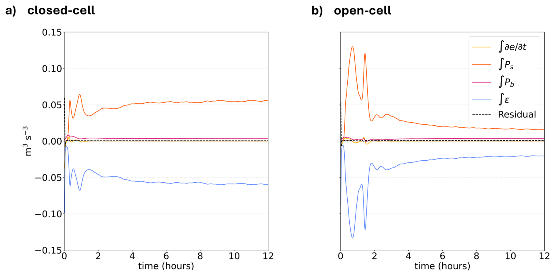
Figure A9 Subgrid-scale TKE budget. Panel (a) shows results for the closed-cell detailed case, and panel (b) for the detailed open-cell case. All terms are spatially averaged.

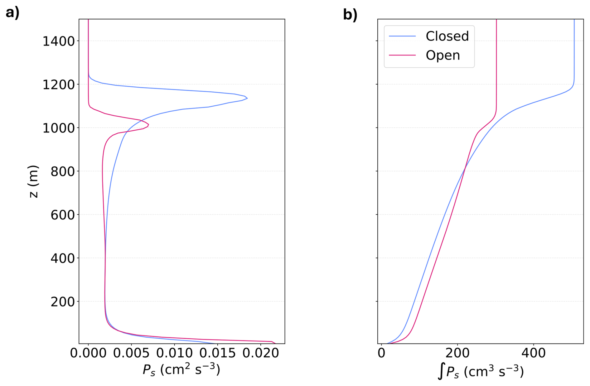
Figure A10 Vertical profiles of subgrid-scale TKE shear production. Panels (a) and (b) show profiles for the detailed simulations, averaged over the last 1 h. Panel (a) shows the slab-averaged vertical distribution (tendency), while panel (b) shows the slab-averaged cumulative vertical integral.

Appendix B: Reconstruction of effective relative humidity

Here we describe how we estimate the irreversible entropy production associated with evaporation using only horizontally averaged variables, since we have access to the full 3D fields for only two simulations in the ensemble. To do so, we must estimate the effective relative humidity of evaporation R_eff defined in Eq. (16). A starting point is to use the horizontally averaged mean relative humidity profile $\stackrel{\mathrm{‾}}{R}$. However, as shown in Fig. A7, this produces a substantial under estimate of the relative humidity at which evaporation occurs in the entrainment layer just above the cloud top. Instead, we perform a simple fitting procedure for the difference between the $\stackrel{\mathrm{‾}}{R}$ and ${\stackrel{\mathrm{‾}}{R}}_{\text{eff}}$ that depends on the inversion height and strength. Specifically, we define a reconstructed relative humidity ${\stackrel{\mathrm{‾}}{R}}_{\text{rec}}$ so that

$$\begin{array}{}\text{(B1)}& {\displaystyle }{\displaystyle }{\stackrel{\mathrm{‾}}{\log \left(R\right)}}_{\text{rec}}=\stackrel{\mathrm{‾}}{\log \left(R\right)}+A\exp [-({\displaystyle \frac{z-z_{\mathrm{0}}}{w}}{)}^n],\end{array}$$

with fitting parameters approximated by

$$\begin{array}{}\text{(B2)}& {\displaystyle }& {\displaystyle }{z}_{\mathrm{0}}=z_{\text{inv}}+(z_{\text{inv}}-z_{\text{ct}}),\text{(B3)}& {\displaystyle }& {\displaystyle }w=z_{\text{inv}}-z_{\text{ct}},\text{(B4)}& {\displaystyle }& {\displaystyle }A={\displaystyle \frac{\mathrm{2}}{\mathrm{3}}}\mathrm{\Delta }\stackrel{\mathrm{‾}}{\log \left(R\right)},\end{array}$$

where z_inv and z_ct are the inversion height and cloud-top height, respectively, and $\mathrm{\Delta }\stackrel{\mathrm{‾}}{\log \left(R\right)}$ is the jump in $\stackrel{\mathrm{‾}}{\log \left(R\right)}$ at the inversion. We find that approximating z_inv with the middle point in the inversion jump for the relative humidity profile works best for the reconstruction. The exponent n is fixed at 2.7, and the fit is obtained via a least-squares procedure.

Using ${\stackrel{\mathrm{‾}}{\log \left(R\right)}}_{\text{rec}}$, we now estimate the entropy production associated with evaporation as

$$\begin{array}{}\text{(B5)}& {\displaystyle }{\displaystyle }{\dot{s}}_{\mathrm{i}}^{\text{evap}}=\underset{z}{\int }\stackrel{\mathrm{‾}}{E}{\stackrel{\mathrm{‾}}{\log \left(R\right)}}_{\text{rec}}\mathrm{d}z\end{array}$$

This equation depends only on horizontally averaged terms, and therefore may be calculated for all ensemble members.

Figure A7 illustrates this reconstruction for the detailed closed-cell simulation, showing the quality of the fit and of the reconstruction. In Fig. A8 we show the procedure applied to a random ensemble member, for which 3D output is not available.