The impact of aerosol mixing state on immersion freezing: insights from classical nucleation theory and particle-resolved simulations

Immersion freezing, initiated by ice-nucleating particles (INPs) in supercooled aqueous droplets, plays an important role in the formation of ice crystals within clouds. The efficiency of immersion freezing depends strongly on INP composition and, crucially, on the mixing state – how chemical species are distributed across the particle population. Here, we quantify the impact of aerosol mixing state on immersion freezing using a combined theoretical and particle-resolved modeling approach. We derive analytical expressions for the frozen fraction of internally and externally mixed INP populations based on classical nucleation theory, showing that the frozen fraction is sensitive to whether ice-active species are present in all particles or only in a subset of the population. We introduce a multi-species immersion freezing scheme into the particle-resolved model PartMC, using the water activity-based immersion freezing model (ABIFM) to compute freezing probabilities for mixed-composition particles. To improve computational efficiency, we implement a Binned Tau-Leaping algorithm and demonstrate an order-of-magnitude speedup with minimal accuracy loss. Simulations reproduce the analytical trends in limiting cases and extend the analysis to more general aerosol populations, where mixing state continues to exert a substantial control on frozen fraction. Sensitivity analyses across particle size, species type, and cooling condition reveal that the mixing state effect is most pronounced when small amounts of highly efficient INPs are mixed with less efficient materials. These findings underscore the need to represent aerosol mixing state explicitly in models of heterogeneous ice nucleation to reduce uncertainty in cloud-phase partitioning.

1 Introduction

Atmospheric aerosols are chemically complex mixtures whose composition reflects both source diversity and chemical aging during transport. Single-particle and chemical imaging studies have shown that individual particles often contain multiple components and exhibit substantial particle-to-particle variability (e.g., Murphy and Thomson, 1997; Laskin et al., 2016, 2019), while laboratory, field, and review studies have documented how atmospheric processing transforms aerosol composition over time (e.g., Rudich, 2003; Hodshire et al., 2019). This compositional diversity is commonly described in terms of aerosol mixing state, which spans a continuum from extreme externally mixed to extreme internally mixed populations. In an extreme external mixture, each particle consists of a single chemical species, whereas in an extreme internal mixture, all particles share the same composition (Winkler, 1973). For brevity, these two limiting cases are hereafter referred to as external and internal mixtures. Aerosol mixing state influences several climate-relevant properties by altering how chemical constituents are distributed across particles. For example, previous studies have shown that mixing state affects cloud condensation nuclei (CCN) activity through its influence on particle hygroscopicity and size-resolved composition (Deng et al., 2013; Ren et al., 2018; Wang et al., 2018; Rejano et al., 2024), and modifies aerosol optical properties through changes in the spatial association of absorbing and scattering material within particles (e.g., Lesins et al., 2002; Liu and Mishchenko, 2018; Zheng et al., 2021). However, its role in heterogeneous ice nucleation remains comparatively underexplored, which motivates the present study.

Ice nucleating particles (INPs) are aerosol particles that facilitate ice crystal formation by lowering the energy barrier for ice nucleation (Pruppacher and Klett, 1996; Knopf and Alpert, 2023). This process allows ice to form at higher temperatures than would be possible through homogeneous nucleation. INPs play a critical role in mixed-phase clouds by altering the water-to-ice content ratio, thereby influencing both cloud glaciation and precipitation formation (Pruppacher and Klett, 1996; Lohmann, 2002; Ansmann et al., 2008; Kanji et al., 2017; Storelvmo, 2017). This modulation of the water-to-ice content ratio also affects radiative transfer within mixed-phase clouds (McCoy et al., 2014a, b, 2016; Murray et al., 2021), which is a key factor in regulating the Earth's radiative balance.

Numerous studies highlight the importance of aerosol chemical composition in heterogeneous ice nucleation (e.g., Möhler et al., 2008; Phillips et al., 2008; Knopf et al., 2018; Joghataei et al., 2020). The chemical and physical properties of aerosol species strongly influence their effectiveness as INPs, including surface structure (e.g., Fitzner et al., 2015; Kiselev et al., 2017; Yang et al., 2018), surface chemistry (e.g., Diehl and Mitra, 1998; Zuberi et al., 2002; Knopf et al., 2014; Wang et al., 2016), and hydrophilicity or hydrophobicity (e.g., Fitzner et al., 2015; Bi et al., 2016). Laboratory and modeling studies have shown that heterogeneous ice nucleation efficiency varies substantially across aerosol species, in some cases by several orders of magnitude under similar environmental conditions (Diehl and Mitra, 1998; Murray et al., 2012). This variability has been linked to differences in particle surface properties, nucleation mechanisms, and water-activity-related effects (Knopf and Alpert, 2013; Knopf et al., 2018; Wagner et al., 2021). Since the mixing state determines how chemical species with varying ice nucleation efficiencies are distributed within an aerosol population, it plays a crucial role in the overall frozen fraction of INPs. Figure 1 illustrates this effect by comparing two groups of INPs of the same size, each featuring two surface species: gray represents a highly efficient ice nucleating species (“good nucleator”), while green denotes a less effective ice nucleating species (“bad nucleator”). The group on the left represents an external mixture, where each particle consists of a single species, whereas the group on the right is an internal mixture, with both species present in each particle. During cooling, assuming the INPs are immersed in water, only the particles that contain the good nucleator will transition to ice in the external mixture. In contrast, in the internal mixture, the presence of the good nucleator in all particles enables the entire population to freeze. This mechanism results in a 50 % difference in ice formation, underscoring the significant impact of aerosol mixing state on ice crystal formation.

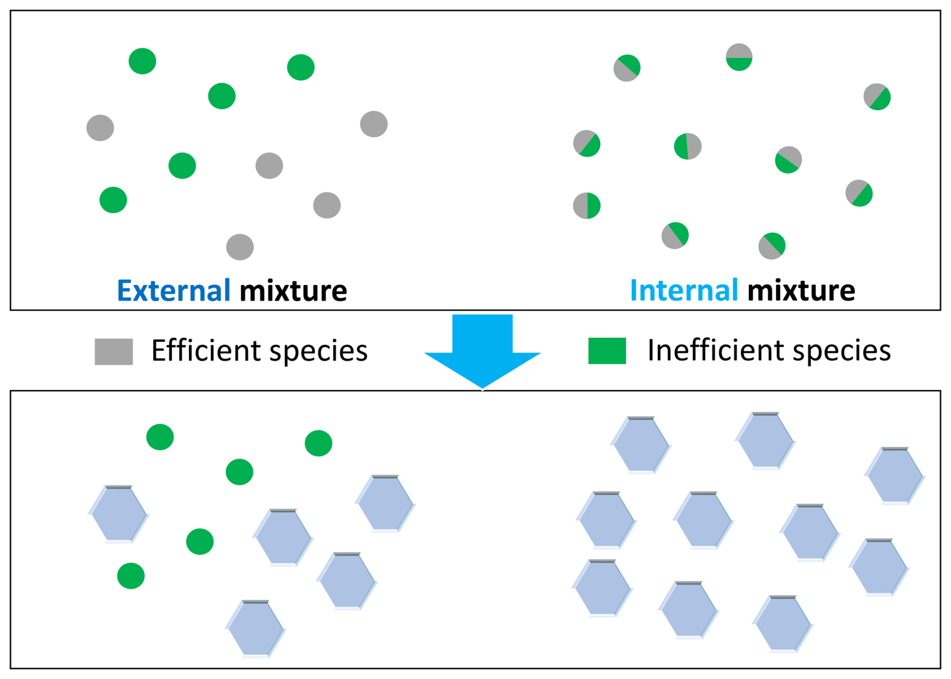
Figure 1 An example highlighting how mixing states affect the amount of ice formation. The top panel shows the INPs given at initial stage, with 50 % of the INPs effective at freezing (gray) and 50 % ineffective (green), distributed as both external and internal mixtures. The bottom panel displays the result after a certain duration, where the effective INPs in the internal mixture have induced a more widespread ice formation, as represented by the hexagons, compared to the external mixture.

Several studies have investigated the INP mixing state impact on ice nucleation, with most focusing on changes due to chemical ageing, particularly through the coating process (Kanji et al., 2017; Knopf et al., 2018). Laboratory studies have shown that when dust particles are coated with organic material or sulfuric acid, their effectiveness as INPs is significantly reduced (Möhler et al., 2008; Sullivan et al., 2010; Kanji et al., 2017; Stevens and Dastoor, 2019). Xue et al. (2024) experimentally quantified the relative errors in contact angle measurements for sea salt particles with different mixing state during deposition ice nucleation. Their findings suggest that both the particle composition and mixing state influence the ice-nucleating abilities of marine aerosols. Similarly, Spichtinger and Cziczo (2010) used box model simulations to examine differences in deposition freezing between internally and externally mixed INPs in cirrus clouds. The study found that the contrast in freezing ability between these two mixing states was more pronounced than the difference between size-dependent and size-independent nucleation threshold assumptions.

Two general approaches are commonly used to describe heterogeneous ice nucleation in atmospheric models: the singular approach (Hoose and Möhler, 2012; Niedermeier et al., 2015; Shima et al., 2020; Abade and Albuquerque, 2024) and the time-dependent approach (Fletcher, 1958, 1959, 1962; Koop et al., 2000; Knopf and Alpert, 2013; Alpert and Knopf, 2016; Knopf and Alpert, 2023), the latter based on classical nucleation theory (CNT). The singular approach assumes that each droplet freezes at a characteristic temperature, independent of time, while the time-dependent formulation treats freezing as a stochastic process governed by a temperature-dependent nucleation rate. Both frameworks are simplifications of a more complex reality, and ongoing research continues to evaluate their respective merits. Notably, Arabas et al. (2025) conducted a systematic comparison using prescribed-flow simulation and found that the CNT-based approach yields more robust results across a range of cooling conditions. This is particularly evident when laboratory-derived nucleation parameters are applied. In this study, we adopt the CNT-based, time-dependent framework to describe immersion freezing, both for its theoretical grounding and its compatibility with our particle-resolved modeling strategy. However, the compatibility of our theoretical framework with singular/INAS-based formulations is discussed in the Discussion section.

While previous studies have suggested that aerosol mixing state can influence ice nucleation, the underlying mechanisms remain poorly constrained. Laboratory and field observations have shown that particle coatings, morphology, and surface composition can all affect heterogeneous ice nucleation by altering active sites and water uptake behavior (e.g., Baustian et al., 2012; Lata et al., 2021), but these effects are often difficult to disentangle. In addition, earlier studies have represented heterogeneity in freezing behavior through variability in site-specific nucleation properties within or across particles (e.g., Niedermeier et al., 2011), yet quantitative investigations that isolate the effect of particle-to-particle compositional mixing state remain scarce. In many cases, changes in mixing state occurred alongside chemical aging or coating processes that also modified particle composition and the surface area contributions of different species, making it difficult to separate the direct effect of mixing state from concurrent changes in particle properties. To our knowledge, no particle-resolved modeling study has systematically quantified the effect of compositional mixing state on freezing behavior while controlling for these confounding factors.

In this study, we do not seek to represent a specific atmospheric transformation pathway, such as coating-driven aging from an external to an internal mixture. Instead, we ask a controlled sensitivity question: for aerosol populations with the same bulk composition and size distribution, how does predicted immersion freezing depend on how constituent species are distributed across particles, from external to internal mixing? This framing isolates the role of mixing-state representation while holding other population-level properties fixed. This question is particularly relevant for ice nucleation modeling, where model inputs typically describe the bulk amounts of aerosol species but do not explicitly resolve particle-level mixing state. As a result, freezing predictions can depend on how this unresolved mixing state is represented.

To address this question, we first develop a theoretical framework based on classical nucleation theory to quantify the sensitivity of the frozen fraction to the INPs' mixing state during the immersion freezing process. We then design and implement particle-resolved immersion freezing simulations within the Particle-resolved Monte Carlo Model (PartMC, Riemer et al., 2009). This approach provides a precise and flexible representation of different mixing states, allowing us (i) to confirm that the numerical implementation reproduces the analytical predictions in limiting cases where closed-form results are available, and (ii) to extend the analysis to more general aerosol populations, including polydisperse cases, for which an analytical treatment is not feasible.

2 Classical nucleation theory for mixed particles

Following classical nucleation theory, heterogeneous ice nucleation occurs when the first nucleation event on the surface of an ice nucleus triggers the entire droplet to freeze. These events are stochastic Poisson processes (Pruppacher and Klett, 1996; Koop et al., 1997; Leonard and Im, 1999; Consiglio et al., 2023; Knopf and Alpert, 2023). The probability of ice nucleation within a small time step Δt assuming a constant nucleation rate λ is given by

$$\begin{array}{}\text{(1)}& P_{\text{frz}}\left(\mathrm{\Delta }t\right)=\mathrm{1}-e^{-\mathit{\lambda }\mathrm{\Delta }t},\end{array}$$

where λ (unit: s⁻¹) depends on the size and material of the ice nucleus, as well as ambient conditions, including temperature, vapor pressure, and the properties of solutions in cases where an INP is immersed in a droplet. If λ varies over time, the probability over a period t becomes

$$\begin{array}{}\text{(2)}& P_{\text{frz}}\left(t\right)=\mathrm{1}-e^{-{\int }_{\mathrm{0}}^t\mathit{\lambda }\left(\mathit{\tau }\right)\mathrm{d}\mathit{\tau }},\end{array}$$

as described by Koop et al. (1997); Leonard and Im (1999); Consiglio et al. (2023), and detailed in Appendix A1. Since classical nucleation theory assumes that nucleation events occur randomly on the nucleus surface, λ is proportional to the surface area. This leads to the definition of the heterogeneous nucleation rate coefficient J_het (unit: ${\mathrm{m}}^{-\mathrm{2}}{\mathrm{s}}^{-\mathrm{1}}$), which quantifies the expected number of nucleation events per unit surface area per unit time. For an INP of surface area S_p, the relationship is

$$\begin{array}{}\text{(3)}& \mathit{\lambda }=J_{\text{het}}\cdot S_{\mathrm{p}}.\end{array}$$

The heterogeneous nucleation rate coefficient J_het depends on environmental conditions and the inherent properties of the INP. If the surface comprises regions with differing nucleation efficiencies – that is, some parts actively nucleate ice while others do not – Eq. (3) can be extended to an integral over the entire surface area:

$$\begin{array}{}\text{(4)}& \mathit{\lambda }={∯}_S{J}_{\text{het}}\left(\mathit{r}\right)\cdot \mathrm{d}S,\end{array}$$

where the vector r indicates a specific point on INP surface. This equation forms the foundation for simulating multi-species ice nucleation per particle. In particle-resolved models, the state of a particle is described by the amounts of its constituent species. The surface area occupied by each species can be determined with assumptions about the particle morphology. For example, under a simple morphological assumption where particles are spherical and the surface area fraction of each species is proportional to its volume fraction, the surface coverage can be estimated from the relative volumes of the constituent species, which can be calculated from their masses and densities. Using this information, the freezing probability within Δt for a droplet containing such an INP can be expressed as

$$\begin{array}{}\text{(5)}& P_{\text{frz}}\left(\mathrm{\Delta }t\right)=\mathrm{1}-e^{-{\overline{J}}_{\text{het}}\cdot S_{\mathrm{p}}\cdot \mathrm{\Delta }t},\end{array}$$

where

$$\begin{array}{}\text{(6)}& {\overline{J}}_{\text{het}}={\displaystyle \frac{\mathrm{1}}{S_{\mathrm{p}}}}\sum _{i=\mathrm{1}}^{N_{\mathrm{s}}}(S_i\cdot J_{\text{het}}^{\left(i\right)})=\sum _{i=\mathrm{1}}^{N_{\mathrm{s}}}{w}_i\cdot J_{\text{het}}^{\left(i\right)},\end{array}$$

is the surface area weighted mean of the nucleation rate coefficient among all N_s species on the surface of the immersed INP, S_i is the immersed surface area covered by the ith species, S_p is the total immersed surface area, and $w_i=S_i/S_{\mathrm{p}}$ is the immersed surface ratio of the ith species. Similarly, the freezing probability within the time range t in the Eq. (2) can be written as

$$\begin{array}{}\text{(7)}& P_{\text{frz}}\left(t\right)=\mathrm{1}-e^{-S_{\mathrm{p}}{\int }_{\mathrm{0}}^t{\overline{J}}_{\text{het}}\left(T\right(\mathit{\tau }\left)\right)\cdot \mathrm{d}\mathit{\tau }}.\end{array}$$

For convenience, we define Φ_i, for each species as

$$\begin{array}{}\text{(8)}& {\mathrm{\Phi }}_i\left(t\right)={\int }_{\mathrm{0}}^t{J}_{\text{het}}^{\left(i\right)}\left(T\right(\mathit{\tau }\left)\right)\mathrm{d}\mathit{\tau },\end{array}$$

so that Eq. (7) can be written in terms of Φ_i as

$$\begin{array}{}\text{(9)}& P_{\text{frz}}\left(t\right)=\mathrm{1}-\exp \left[-S_{\mathrm{p}}\cdot \sum _{i=\mathrm{1}}^{N_{\mathrm{s}}}{w}_i{\mathrm{\Phi }}_i\left(t\right)\right].\end{array}$$

To analyze the impact of the mixing state factor on ice production, other variables affecting the amount of ice production, such as cooling rate and duration, must be controlled. Thus, under the same cooling conditions but varying mixing states, Φ_i serves as a fixed descriptor for a species' freezing capability. Additionally, Eq. (9) provides a convenient representation of Eq. (7) for the theoretical analysis discussed in the following sections.

3 Sensitivity of immersion freezing to aerosol mixing state

In Sect. 2, Eq. (9) introduced the calculation of freezing probabilities for individual multi-species INPs. Building on this, this section examines the macroscopic frozen fraction of a multi-species INP population emphasizing the impact of mixing state on the frozen fraction. The goal is to quantify the sensitivity of the frozen fraction to aerosol mixing state during immersion freezing. The analysis focuses on monodisperse particles, with the impact on polydisperse particles left for future studies.

Even when two INP populations share the same particle count, particle sizes, and species surface area, and experience the same cooling rate, their frozen fractions can differ due to differences in mixing state. For a given scenario, we define this sensitivity as:

$$\begin{array}{}\text{(10)}& \text{Sensitivity}={\displaystyle \frac{f_{\text{frz}}^{\text{(max)}}-f_{\text{frz}}^{\text{(min)}}}{f_{\text{frz}}^{\text{(max)}}}}\cdot \mathrm{100}\mathit{\%}.\end{array}$$

Here, $f_{\text{frz}}^{\text{(max)}}$ and $f_{\text{frz}}^{\text{(min)}}$ are the maximum and minimum frozen fraction values across all mixing states for the given scenario. The mixing state that produces the highest frozen fraction is referred to as the most efficient mixing state, while the one resulting in the minimum frozen fraction is termed the least efficient mixing state. The magnitude of sensitivity can also be viewed as an upper bound of the relative error in frozen fraction calculations caused by uncertainties in the mixing state.

Here, we present a theorem regarding the most and least efficient mixing states for this scenario.

Theorem 1.

For monodisperse INP populations, the internal mixture is the most efficient mixing state, while the external mixture is the least efficient mixing state.

The proof is shown in Appendix D. Therefore, we have $f_{\text{frz}}^{\text{(max)}}=f_{\text{frz}}^{\text{(int)}}$, and $f_{\text{frz}}^{\text{(min)}}=f_{\text{frz}}^{\text{(ext)}}$, where $f_{\text{frz}}^{\text{(int)}}$ and $f_{\text{frz}}^{\text{(ext)}}$ are the frozen fractions corresponding to internal and external mixtures, respectively. As shown in Eq. (10), the sensitivity of monodisperse INPs depends entirely on the frozen fractions of internal and external mixture, emphasizing the need to study their differences.

It should be emphasized that Theorem 1 is only valid when internal and external mixtures of a monodisperse particle population are compared. A counterexample for polydisperse particle populations is discussed in Appendix E. While our framework can be applied to polydisperse populations (as discussed in Sect. 5.3), the distinction between internal and external mixtures is only meaningful within a single size bin – that is, mixing state comparisons are made between particles of the same size, not across different sizes.

Section 3.1 derives theoretical expressions for the frozen fraction of internal and external mixtures and offers physical insights to explain these differences. Section 3.2 examines how sensitivity is influenced by variations in species types, temperature profiles, INP sizes, and species' total surface area ratios.

3.1 Evaluating frozen fractions for internal and external mixtures

Consider an internally mixed, monodisperse INP population composed of multiple species, with N_p particles, each immersed in a supercooled droplet. By the Law of Large Numbers, the expected frozen fraction f_frz equals the arithmetic average of the freezing probabilities of all INPs,

$$\begin{array}{}\text{(11)}& f_{\text{frz}}={\displaystyle \frac{\mathrm{1}}{N_{\mathrm{p}}}}\sum _{j=\mathrm{1}}^{N_{\mathrm{p}}}{P}_{\text{frz,}j},\end{array}$$

where P_frz,j is the freezing probability of the jth INP as expressed in Eq. (9).

Let N_s denote the number of species present in the population, and $w_i=S_i/S_{\mathrm{p}}$ represent the surface area ratio of the ith species, where S_i is the area covered by species i and S_p is the total INP surface area.

For the externally-mixed case, the following applies. Since each particle contains only one species, the whole INP population can be conceptualized as a collection of distinct species. The unfrozen fraction of the whole INP population after time t can be written as

$$\begin{array}{}\text{(12)}& f_{\text{unf}}^{\text{(ext)}}=\sum _{i=\mathrm{1}}^{N_{\mathrm{s}}}{w}_i\cdot f_{\text{unf}}^{\left(i\right)},\end{array}$$

where w_i is the ratio of the total surface area of INPs in the ith mode relative to the total surface area across all INPs and $f_{\text{unf}}^{\left(i\right)}$ is the unfrozen fraction for droplets containing single-species monodisperse INPs, whose surface is 100 % covered by the ith species (for a detailed derivation, see Appendix A2). The frozen fraction is therefore

$$\begin{array}{}\text{(13)}& f_{\text{frz}}^{\text{(ext)}}=\mathrm{1}-\sum _{i=\mathrm{1}}^{N_{\mathrm{s}}}{w}_i\cdot f_{\text{unf}}^{\left(i\right)}=\mathrm{1}-\sum _{i=\mathrm{1}}^{N_{\mathrm{s}}}{w}_i\cdot (\mathrm{1}-f_{\text{frz}}^{\left(i\right)}).\end{array}$$

In contrast, for the internally-mixed case the unfrozen fraction $f_{\text{unf}}^{\text{(int)}}$ can be expressed as

$$\begin{array}{}\text{(14)}& f_{\text{unf}}^{\text{(int)}}=\prod _{i=\mathrm{1}}^{N_{\mathrm{s}}}(f_{\text{unf}}^{\left(i\right)}{)}^{w_i}.\end{array}$$

This form arises because a droplet containing internally mixed INPs remains unfrozen only when none of its surface components nucleates ice. Assuming independent nucleation events, the probabilities of remaining unfrozen multiply, and each term is raised to the power of its surface fraction w_i to account for proportional surface coverage. Thus, this leads us to an expression that relates the frozen fraction of droplets containing internally mixed INPs to a combination of the single-species reference cases,

$$\begin{array}{}\text{(15)}& f_{\text{frz}}^{\text{(int)}}=\mathrm{1}-\prod _{i=\mathrm{1}}^{N_{\mathrm{s}}}(\mathrm{1}-f_{\text{frz}}^{\left(i\right)}{)}^{w_i}.\end{array}$$

Here $f_{\text{frz}}^{\text{(int)}}$ represents the frozen fraction for droplets containing internally mixed INPs, whereas $f_{\text{frz}}^{\left(i\right)}$ denotes the frozen fraction that would occur if the particle surface were entirely covered by the ith INP species (for detailed derivation, see Appendix A3). Equation (14) implies that for monodisperse INPs, the internal mixture's unfrozen fraction is a weighted geometric mean of the single-species counterparts' unfrozen fractions, weighted by the species surface ratio. A mathematical description similar to Eqs. (13) and (15) is also discussed in Broadley et al. (2012).

To recap, Eqs. (13) and (15) explain the differences in ice nucleation between external and internal mixtures. Mathematically, this difference corresponds to the inequality between the arithmetic and geometric means: for any set of positive values that are not all equal, the arithmetic mean exceeds the geometric mean. As a result, internal mixtures generally yield higher frozen fractions than external mixtures. Moreover, the difference between the two increases as the variability among species increases, meaning that the sensitivity of the frozen fraction to the INP mixing state becomes more pronounced when species have diverse freezing efficiencies (i.e., different $f_{\text{unf}}^{\left(i\right)}$).

Despite having the same total surface area covered by a species in both the internal and the external mixture scenario, the difference in ice formation between internal and external mixtures arises because each INP freezes its droplet only once, regardless of its nucleation rate. In external mixtures (Fig. 1, left), the efficient freezing species (“good nucleator”) only covers half of the INPs, so only half of the INPs are highly effective. Once these INPs freeze their droplets, any further nucleation events occurring within these already frozen droplets, though predicted by the theoretical probability model, do not lead to the formation of new ice, rendering the high efficiency of the good nucleators redundant. The remaining half consists of less effective species (“bad nucleator”), leading to fewer freezing events. In contrast, internal mixtures distribute the good nucleator across all INPs, increasing the probability of new nucleation events in unfrozen droplets, producing more ice.

To illustrate the results derived so far, Fig. 2 compares frozen fractions for internally-mixed and externally-mixed monodisperse INP populations consisting of two species, species A and B. We assume that the species each cover 50 % of the total INP surface area. Species A nucleates ice very efficiently with the same J_het as Fe₂O₃, while the J_het ratio of species B to A is varied (shown on the x axis). All frozen fractions are calculated using Eqs. (9), (11), (13), and (15).

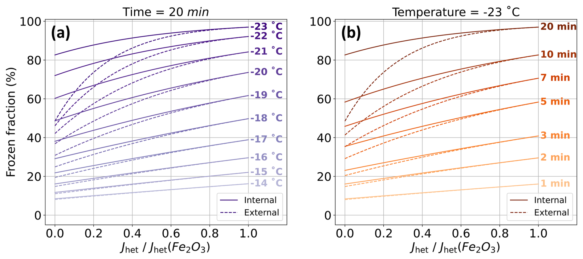
Figure 2 Frozen fractions comparing internally and externally mixed INPs after being exposed to a constant temperature for a certain time t_freeze. (a) Frozen fraction is evaluated for different temperatures with t_freeze=20 min. (b) Frozen fraction is evaluated for different t_freeze at a fixed temperature of −23 °C.

Figure 2a shows the frozen fractions for internal and external mixtures after being exposed to a constant temperature for 20 min, where the temperatures vary from −14 to −23 °C. As expected, the differences are more pronounced at small J_het ratios, where the two species' freezing efficiencies differ strongly. Concurrently, at lower temperatures, the J_het disparity has a larger impact, whereas at higher temperatures, the frozen fractions for both mixtures become nearly identical. Figure 2b shows the frozen fractions over durations from 1 to 20 min at −23 °C. Longer durations show more pronounced differences at small J_het ratios, whereas shorter durations yield negligible differences. The results in both panels show a similar pattern, because lower temperatures and longer durations both lead to higher Φ values, which is the parameter that appears in Eq. (9). Since temperature and duration are combined in Φ, we will use Φ as a simpler parameter to represent freezing ability, avoiding complex cooling conditions with varying temperature profiles.

3.2 Frozen fraction's sensitivity to mixing state

In the previous section, we suggested that using the Φ value simplifies the classification of cooling condition with varying temperature and duration. For example, the condition with a brief duration at low temperatures and those with longer durations at higher temperatures can be considered equivalent if they share the same Φ value. In this section, we continue using the model from Fig. 2 and analyze the effects of INP size and the total surface area fraction of each species on sensitivity of frozen fraction to mixing state.

Figure 3 introduces a sensitivity map for monodisperse INPs with dry diameter of 1 µm, and a surface ratio of two hypothetical species A and B of 50 %. The x and y axis are analogous to Fig. 2 but using Φ instead of J_het for the reasons stated above. Each data point in the sensitivity map represents the sensitivity value defined by Eq. (10) for a scenario involving species A and B, with exemplary Φ values denoted as Φ_A and Φ_B, respectively.

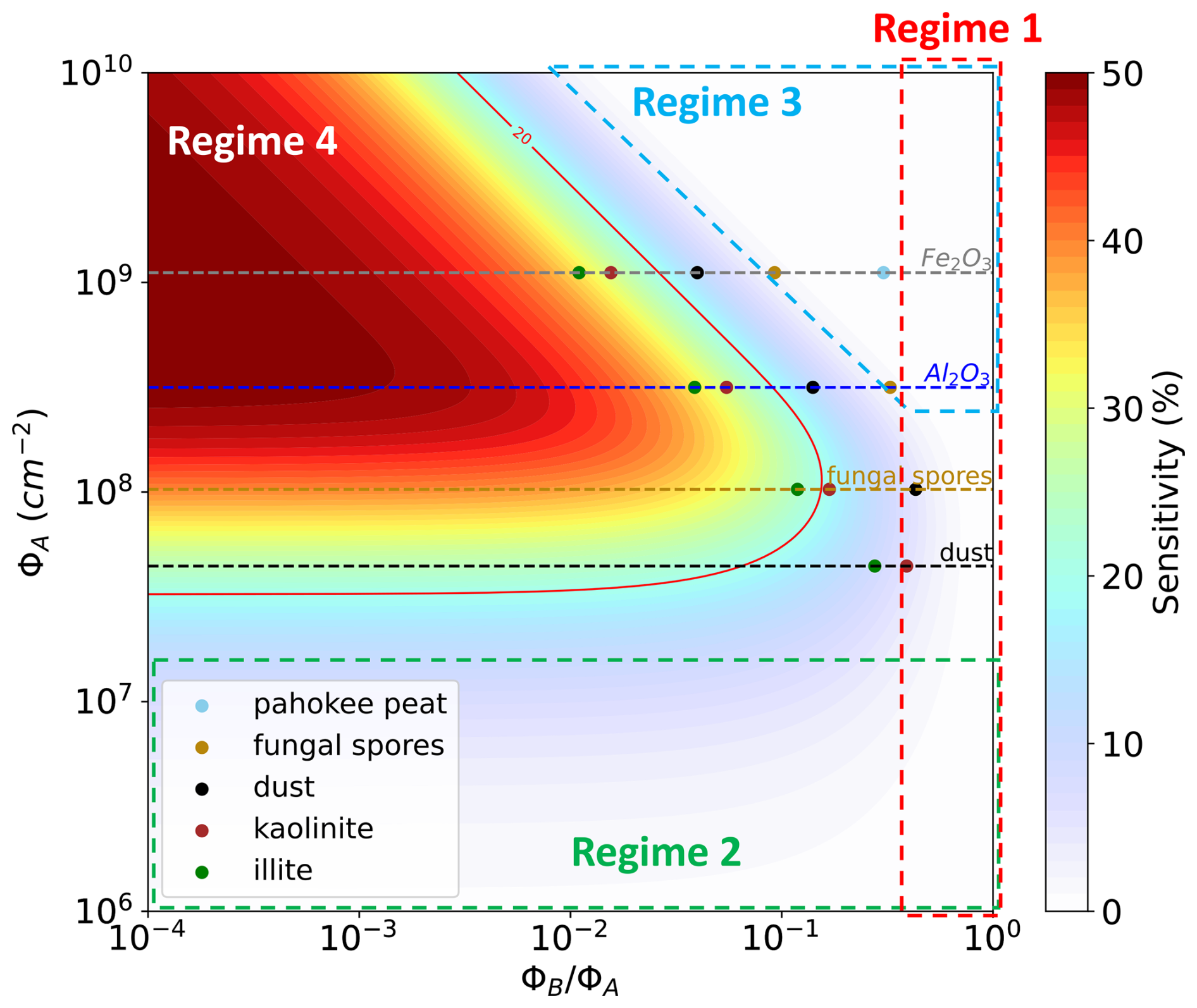
Figure 3 Sensitivity map for particles with a dry diameter of 1 µm, where species A and B are present in a 50:50 ratio. The Φ values are calculated for a scenario with a constant temperature of −33 °C and a duration of 10 min using Eq. (8). The Φ values for Fe₂O₃, Al₂O₃, fungal spores, and dust representing species A are marked by gray, blue, brown, and black horizontal dashed lines, respectively. The sky blue, brown, black, red, and green solid dots along each horizontal line represent the corresponding Φ ratios of pahokee peat, fungal spores, dust, kaolinite, and illite as species B in combination with each species A, respectively. Parameters for ice nucleation calculation are derived from Knopf and Alpert (2013) (listed in Table B1).

For reference, some examples of species combinations A and B are highlighted as horizontal dashed lines and aligned solid dots. For example, the combination of Fe₂O₃ and illite is represented by the green solid dot aligned with the gray dashed line. The Φ values for each species marked in Fig. 3 are calculated for a scenario with a constant temperature of −33 °C and a duration of 10 min, using Eq. (8). The J_het values for each species are computed using the Water Activity-Based Immersion Freezing Model (Knopf and Alpert, 2013), which is explained in more detail in Sect. 4.2. In Fig. 3, there are three regimes where sensitivities are negligible, labeled as Regimes 1 to 3, and marked with red, green, and sky blue boxes, respectively.

Regime 1 represents the scenarios where two species have freezing efficiency close to each other, which results in negligible sensitivity, as discussed in Fig. 2. To explain the small sensitivities in Regimes 2 and 3, we use a simple mathematical analysis. Based on Eq. (9), the unfrozen fraction of monodisperse INPs covered by single species of A or B can be formulated as $f_{\text{unf}}^{\text{(A)}}=\exp (-S_{\mathrm{p}}{\mathrm{\Phi }}_{\mathrm{A}})$ and $f_{\text{unf}}^{\text{(B)}}=\exp (-S_{\mathrm{p}}{\mathrm{\Phi }}_{\mathrm{B}})$, where the $S_{\mathrm{p}}=\mathit{\pi }{D}_{\mathrm{p}}^{\mathrm{2}}$ is the dry surface area of each immersed INP. Therefore, based on Eqs. (12) and (14), the unfrozen fraction of internal mixture, denoted as $f_{\text{unf}}^{\text{(int)}}$, can be expressed as

$$\begin{array}{}\text{(16)}& f_{\text{unf}}^{\text{(int)}}=\exp \left[-{\displaystyle \frac{\mathrm{1}}{\mathrm{2}}}{S}_{\mathrm{p}}\cdot \left({\mathrm{\Phi }}_{\mathrm{A}}+{\mathrm{\Phi }}_{\mathrm{B}}\right)\right],\end{array}$$

while the unfrozen fraction of external mixture, denoted as $f_{\text{unf}}^{\text{(ext)}}$, can be expressed as

$$\begin{array}{}\text{(17)}& f_{\text{unf}}^{\text{(ext)}}={\displaystyle \frac{\mathrm{1}}{\mathrm{2}}}\cdot \left[\exp (-S_{\mathrm{p}}{\mathrm{\Phi }}_{\mathrm{A}})+\exp (-S_{\mathrm{p}}{\mathrm{\Phi }}_{\mathrm{B}})\right].\end{array}$$

In the Regime 2, both species A and B have a relatively small Φ value of less than 10⁷ cm⁻², where the product of S_p and Φ is less than the order of 10⁻¹, resulting in

$$\begin{array}{}\text{(18)}& f_{\text{unf}}^{\text{(int)}}\approx f_{\text{unf}}^{\text{(ext)}}\approx \mathrm{1}-{\displaystyle \frac{\mathrm{1}}{\mathrm{2}}}{S}_{\mathrm{p}}\cdot \left({\mathrm{\Phi }}_{\mathrm{A}}+{\mathrm{\Phi }}_{\mathrm{B}}\right),\end{array}$$

which explains the small frozen fraction difference between internal and external mixtures in this case. In this regime, the result also has a simple physical interpretation. Multiplying Eq. (18) by the total number of particles N_p shows that the expected number of ice particles is approximately equal to the expected number of ice-nucleation triggering events. When nucleation probabilities are small, each triggering event typically leads to the freezing of a single particle. Since the total surface area of each species is the same for internal and external mixtures, the expected number of triggering events is also the same regardless of the mixing state. As a result, the number of frozen particles is nearly identical for the two mixing states, leading to the small sensitivity observed in Regime 2. This result is consistent with Fig. 2 for the conditions of higher temperature and shorter duration time.

In Regime 3, both species A and B have a large Φ value, larger than 10⁸ cm⁻², with the product of S_p and Φ being larger than the order of 10⁰, resulting in

$$\begin{array}{}\text{(19)}& f_{\text{unf}}^{\text{(int)}}\approx f_{\text{unf}}^{\text{(ext)}}\approx \mathrm{0}.\end{array}$$

This indicates a frozen fraction of nearly 100 % for both internal and external mixtures, again resulting in a small difference between the two mixing states.

Regime 4 is where the sensitivity to mixing state is significant (exceeding approximately 20 %, as indicated by the red contour in Figs. 3–5). In this regime, the good nucleator (species A) is efficient at freezing, and a large disparity in freezing efficiency exists between the good nucleator and the bad nucleator (species B). There are several examples of species combinations that fall into Regime 4, such as Fe₂O₃ mixed with illite (34.1 % of sensitivity), Fe₂O₃ mixed with kaolinite (29.0 %), Al₂O₃ mixed with illite (33.7 %), and dust mixed with Pahokee Peat (12.2 %), among others.

From a physical perspective, the differences among these regimes can be understood in terms of how ice-nucleation triggering events are distributed among particles. For a given cooling condition and fixed total surface area of each species, the expected total number of triggering events in the particle population is approximately independent of the mixing state. The mixing state instead determines how these events are distributed among particles. Because only the first triggering event on a particle causes droplet freezing, additional events occurring on the same particle are effectively wasted. Section 3.1 explains the difference between external and internal mixtures precisely from this perspective. In Regime 2, nucleation rates of both species are very small, so the expected number of triggering events per particle is much less than one. Multiple events on the same particle are therefore rare, little waste occurs, and the mixing state has negligible influence on the frozen fraction. In Regime 3, nucleation rates of both species are very large, and each particle surface experiences many triggering events. Even if the nucleation efficiencies of the two species differ by several orders of magnitude, the bad species still produces multiple triggering events on particles composed solely of that species. Consequently, the frozen fraction approaches unity (≈ 100 %) for both internal and external mixtures, because the additional events generated by the good species are effectively wasted once a particle has already frozen. Only in the Regime 4 does the mixing state become important. In this case, particles containing the good species generate more than one triggering event on average, while particles composed of the bad species generate fewer than one. Internal mixing distributes these excess events across particles and reduces waste, whereas external mixtures concentrate them on particles that already freeze easily, leading to a larger difference in frozen fraction.

Figure 4 presents the same sensitivity map as Fig. 3 but for varying INP sizes, ranging from Accumulation mode (D_p=0.1 µm) to coarse mode (D_p=10 µm). The pattern in the figure exhibits a vertical shift with changes in INP size: as the INP size decreases, the pattern shifts upward. In the case of smaller INPs (panels a and b), the immersed surface area of each INP is small, making it difficult for even efficient species to trigger multiple ice nucleation events on the same particle. As a result, Regime 2 dominates the entire sensitivity map. Conversely, for larger INPs with larger immersed surfaces, inefficient species can trigger multiple ice nucleation events, leading to the disappearance of Regime 2 and the dominance of Regimes 1, 3, and 4.

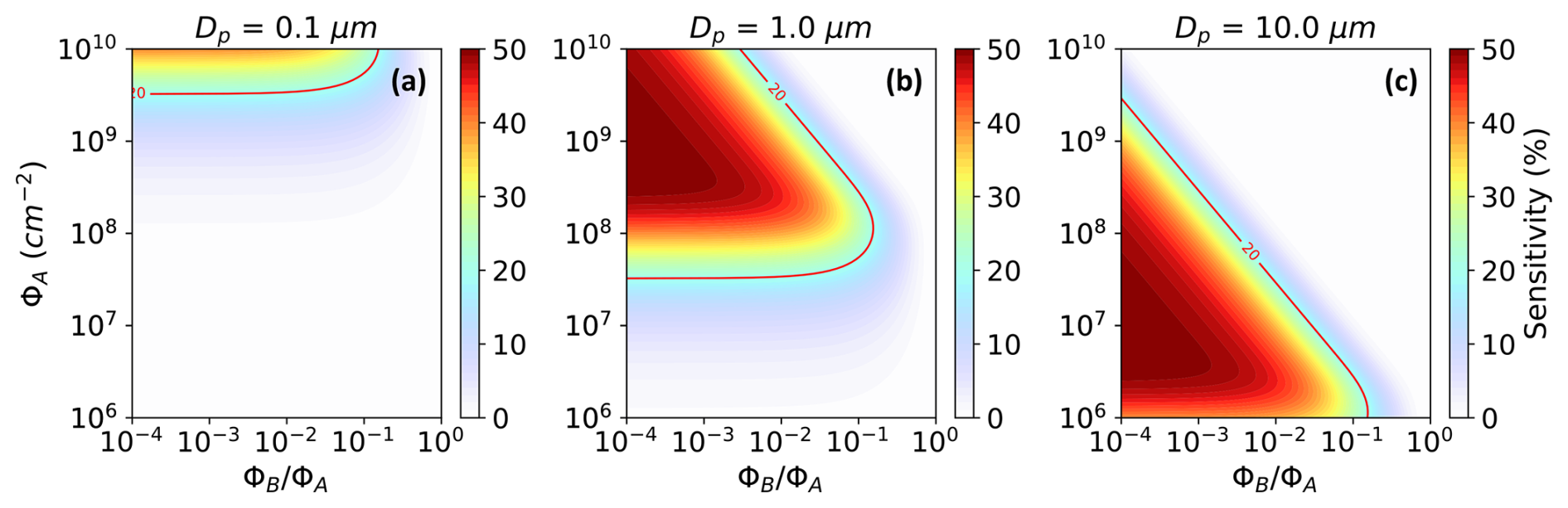
Figure 4 Same as Fig. 3 but with different dry diameter of INPs. (a) 0.1 µm; (b) 1.0 µm; (c) 10 µm.

Figure 5 shows the same sensitivity map as Fig. 3, but for varying immersed surface ratios of species A and B. When the total immersed surface ratio of the efficient ice nucleating species (species A) is small (Fig. 5a), the sensitivity increases across the entire map, especially in Regime 4, where the maximum sensitivity reaches 90 %. In contrast, as the total immersed surface ratio of the efficient ice nucleating species increases, the sensitivity decreases accordingly. Once the surface ratio of species A is 90 %, the maximum sensitivity is reduced to only 10 %. These results indicate that when a mixed-INP population contains a small proportion of highly efficient species, the influence of the mixing state becomes significant, and failure to accurately estimate the mixing state can lead to high error in the frozen fraction calculation.

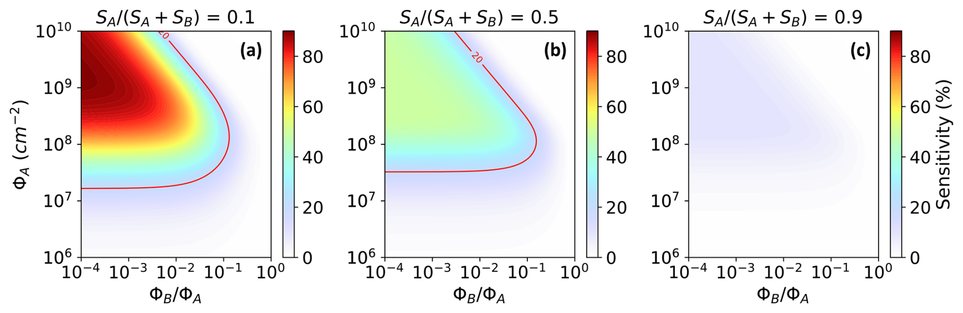
Figure 5 Same as Fig. 3 but with different total immersed surface ratio of species A (i.e., $S_{\mathrm{A}}/(S_{\mathrm{A}}+S_{\mathrm{B}})$). (a) 0.1; (b) 0.5; (c) 0.9.

The influence of mixing state can also be interpreted in terms of changes in the INP spectrum, i.e., the temperature dependence of freezing efficiency. Figure 6 presents the predicted frozen fraction as a function of temperature for different mixing states under a constant cooling rate (ccr), showing that external and internal mixtures define lower and upper bounds of the INP spectrum for a given bulk surface area composition.

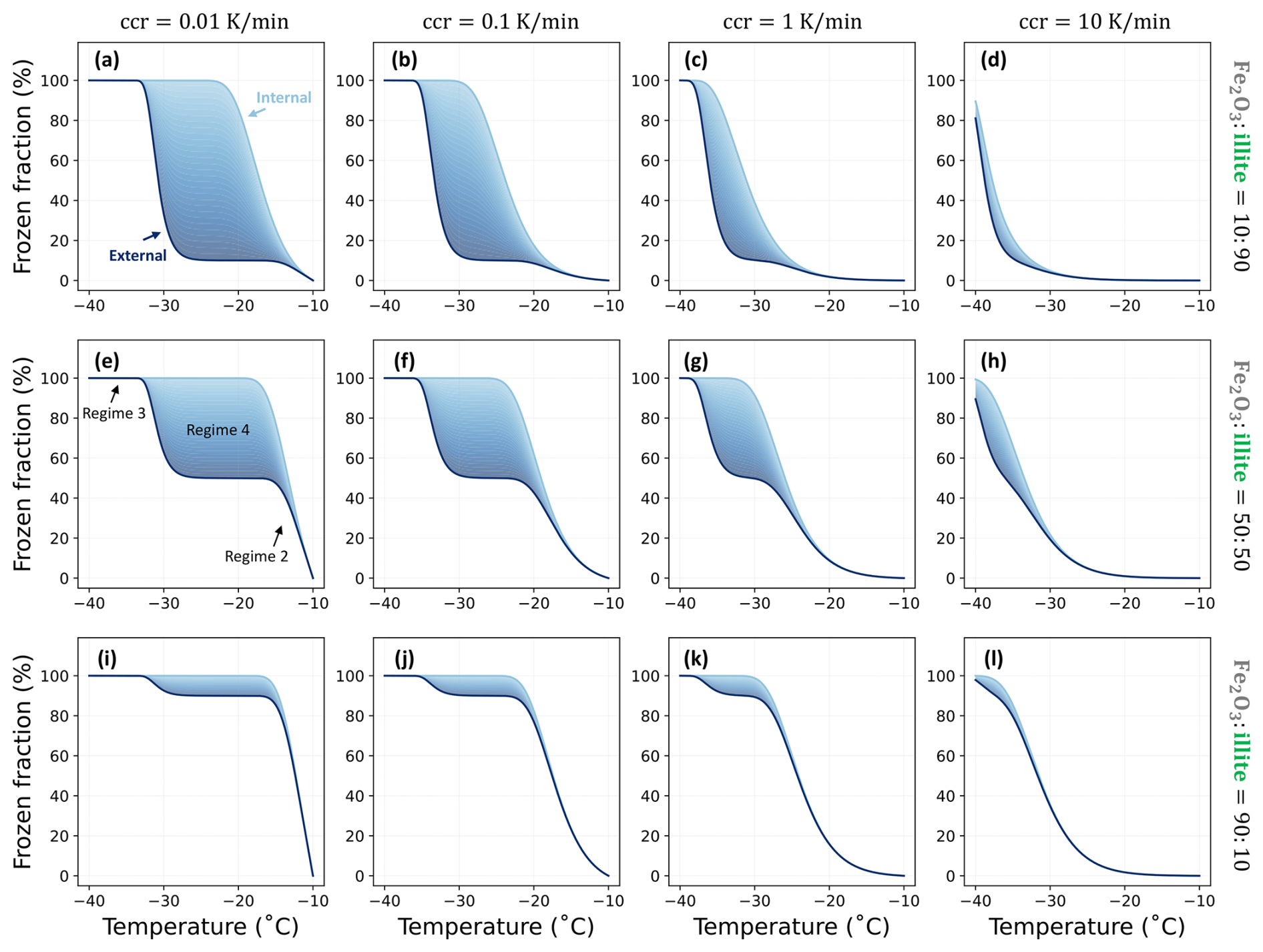
Figure 6 Effect of aerosol mixing state on the frozen fraction predicted by Eqs. (13) and (15) under constant cooling. Each panel shows the frozen fraction as a function of temperature during cooling from −10 to −40 °C. Columns correspond to different ccr, and rows correspond to different surface-area fractions of Fe₂O₃ and illite, with particle diameter fixed at 1 µm. The dark and light boundary curves represent the limiting externally and internally mixed states, respectively, and the shaded region indicates the maximum range of the mixing-state effect. Panel (e) highlights examples of Regimes 2, 3, and 4, similar regime patterns appear across all panels.

It is important to note that the theoretical analysis presented in this section applies to mixtures of insoluble ice-nucleating species only. When soluble species are present in mixed particles, their influence on immersion freezing arises through different mechanisms. After dissolution, soluble species do not contribute nucleating surface area but instead modify the nucleation efficiency of insoluble species through changes in water activity (Knopf and Alpert, 2013). In addition, soluble species can affect the activation of particles into cloud droplets through their hygroscopic properties (Petters and Kreidenweis, 2007), which is a prerequisite for immersion freezing. These processes introduce additional couplings between particle composition, nucleation efficiency, and droplet activation that are not represented in the present theoretical framework. Investigating the role of mixing state in systems containing both soluble and insoluble species therefore requires an extension of the theory developed here and is left for future work.

4 Numerical implementation to particle-resolved model

Section 2 presented the immersion freezing probability for an individual mixed particle, while Sect. 3 analyzed the sensitivity of the frozen fraction to the mixing state of INPs. Starting from this section, we extend the theoretical framework by implementing it within the particle-resolved aerosol model (PartMC). We perform immersion freezing simulations for both single-species and multi-species INPs to confirm the results from Sect. 3 and further investigate the influence of INP mixing state on the frozen fraction. Section 4.1 focuses on the algorithm design for particle-resolved immersion freezing simulations, while Sect. 4.2 presents the simulation setup and results.

4.1 The Particle-resolved Monte-Carlo Model (PartMC)

The particle-resolved Monte Carlo (PartMC) model (Riemer et al., 2009) is a box model for simulating the evolution of aerosol particles in the atmosphere. The volume of interest contains a large quantity of discrete computational particles. Each computational particle represents a sample of real particles with identical properties (DeVille et al., 2011, 2019).

Each computational particle is assumed to be a sphere, and is represented by a vector that contains the masses of the species comprising that particle, i.e., the jth particle is described as ${\mathit{\mu }}_j=({\mathit{\mu }}_{\mathrm{1}}^j,{\mathit{\mu }}_{\mathrm{2}}^j,\mathrm{\dots },{\mathit{\mu }}_{N_{\mathrm{s}}}^j)$, where ${\mathit{\mu }}_i^j$ is the mass of the ith species in the jth particle ($i\in [\mathrm{1},N_{\mathrm{s}}]$), and N_s is the total number of species. Other characteristics of a particle such as the volume of each species, the total mass and the wet diameter (the diameter of the whole particle, including water and dissolved and insoluble aerosol material) and dry diameter (the diameter excluding water) can be derived from its mass vector.

PartMC encompasses multiple physical aerosol processes, including emission of primary aerosols, dilution with background air, coagulation (Riemer et al., 2009), and condensation of water vapor to simulate cloud formation (Ching et al., 2012). Gas-particle partitioning is included when PartMC is coupled with MOSAIC (Zaveri et al., 2008). During these processes, the evolution of the mass of each species in a particle is tracked. This feature makes PartMC a valuable tool for investigating the impact of mixing state on the aerosol population and on climate-relevant properties of the aerosol. The PartMC has been used in several particle-resolved studies, e.g., Kaiser et al. (2011) used PartMC-MOSAIC to simulate the heterogeneous oxidation process on soot particles and derived the half-lives parameter of surface-bound PAHs for large-scale model. Tian et al. (2014) used it to investigate the chemical evolution of aerosols in a ship plume and its impact on CCN properties, Curtis et al. (2017) coupled PartMC-MOSAIC with WRF model to study the vertical distribution of aerosol mixing state during turbulent diffusion and dry deposition within the planetary boundary layer, Hughes et al. (2018) used the mixing state simulation result from PartMC to train the machine learning model for the global estimation of aerosol mixing state distribution, Yao et al. (2022) provided a systematic quantification of mixing state impact on aerosol optical properties based on the PartMC model simulation.

So far, PartMC has not yet been applied to questions related to heterogeneous ice nucleation. In this study, we extended PartMC by including the process of immersion freezing based on classical nucleation theory. Several parameterizations can be used to calculate the heterogeneous nucleation rate coefficient J_het (Fletcher, 1958, 1959, 1962; Pruppacher and Klett, 1996; Phillips et al., 2008; Hoose and Möhler, 2012; Knopf and Alpert, 2013). Following Arabas et al. (2025), we will use the activity-based immersion freezing model (ABIFM) proposed by Knopf and Alpert (2013).

4.2 The water activity-based immersion freezing model (ABIFM) for J_het calculation

The water activity-based immersion freezing model (ABIFM), proposed by Knopf and Alpert (2013), is a useful tool for the estimation of heterogeneous ice nucleation rate J_het in immersion freezing simulations. Following their study, when an INP is immersed in an aqueous solution, the rate coefficient J_het can be determined by the difference of solution water activity a_w and the water activity in equilibrium with ice $a_{\mathrm{w}}^{\text{ice}}$. For an aerosol particle in equilibrium with ambient relative humidity, the numerical value of water activity equals the 100 % of humidity (Koop et al., 2000). The parameterization of J_het is

$$\begin{array}{}\text{(20)}& {\log }_{\mathrm{10}}{J}_{\text{het}}=m\cdot (a_{\mathrm{w}}-a_{\mathrm{w}}^{\text{ice}})+c,\end{array}$$

where, m and c are the ABIFM parameters for a specific aerosol species. Knopf and Alpert (2013) derived the value of m and c for ten different species fitted from experimental data, such as Fe₂O₃, Al₂O₃, fungal spores, dust, 1-Nonadecanol, kaolinite, illite, Leonardite, and Pahokee Peat.

Combining Eqs. (5), (6), and (20), the immersion freezing probability of a supercooled droplet containing one INP with multiple species can be formulated as

$$\begin{array}{}\text{(21)}& {\displaystyle }\left\{\begin{array}{l}{P}_{\text{frz}}=\mathrm{1}-\exp \left[-{\sum }_{i=\mathrm{1}}^{N_{\mathrm{s}}}(w_i\cdot J_{\text{het}}^{\left(i\right)})\cdot S_{\mathrm{p}}\cdot \mathrm{\Delta }t\right];\\ {\log }_{\mathrm{10}}{J}_{\text{het}}=m_{\text{i}}\cdot (a_{\mathrm{w}}-a_{\mathrm{w}}^{\text{ice}})+c_i;\\ a_{\mathrm{w}}=\text{RH}\approx \mathrm{1};a_{\mathrm{w}}^{\text{ice}}=\frac{e_{\mathrm{s}}^{\text{ice}}\left(T\right)}{e_{\mathrm{s}}\left(T\right)};w_i=\frac{S_i}{S_{\mathrm{p}}},\end{array}\right.\end{array}$$

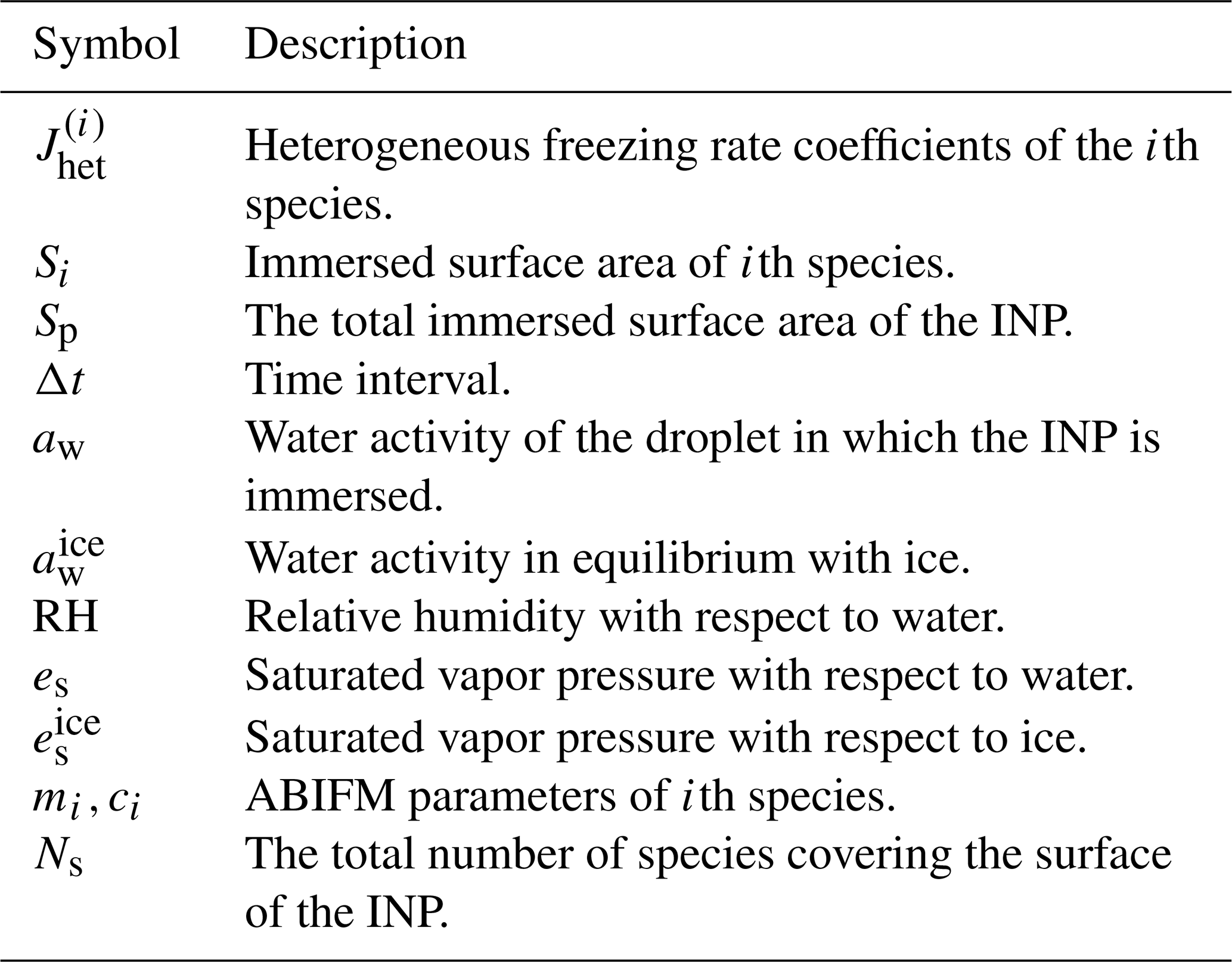
and the descriptions of each variable used in the Eq. (21) are listed in the Table 1.

Table 1 Parameters in Eq. (21).

To use Eq. (21) to calculate the immersion freezing probability of a single droplet with a multi-species insoluble INP, the immersed surface area that each species contributes must be known. However, in PartMC each particle is characterized by the masses of each species, and a detailed description of the particle's morphology is not tracked, and therefore appropriate assumptions need to be made. Here, we assume that the volume ratio of the species equals their surface area ratio, and that all surfaces on the insoluble INP are immersed in water.

The ice nucleation rate coefficient, $J_{\text{het}}^{\left(i\right)}$, is determined by the difference between a_w and $a_{\mathrm{w}}^{\text{ice}}$, along with the parameters m_i and c_i. Assuming the droplet remains in equilibrium with the ambient conditions and the INP it contains is insoluble, hence there is no solute present, the value of a_w is equal to 1. The value of $a_{\mathrm{w}}^{\text{ice}}$ is determined by the ratio of the saturated vapor pressure with respect to ice to the saturated vapor pressure with respect to water. As temperature is the only variable that affects these terms, $a_{\mathrm{w}}^{\text{ice}}$ is thus determined by temperature. The values of m_i and c_i for a specific species are obtained from Knopf and Alpert (2013).

4.3 The implementation to the PartMC model

This section introduces the immersion freezing simulation algorithms that we developed and implemented for the PartMC model. Simulating immersion freezing of a computational particle at a given temperature involves the following five steps (also shown in Algorithm 1):

• #1:

  Check whether the particle has an insoluble component.

• #2:

  Assess whether the temperature is below 0 °C and if that particle is immersed in water.

• #3:

  If a particle meets the above criteria, calculate the freezing probability P_frz using Eq. (21).

• #4:

  Determine whether that particle will freeze at this time step using a stochastic method based on P_frz.

• #5:

  If that particle coagulates with another frozen particle, it will also freeze.

Algorithm 1 Immersion freezing algorithm for one particle.

1:

Given a particle p

2:

if p is soluble then

3:

# The PartMC v2.9.0 does not support ice nucleation for soluble particles.

4:

state(p)←unfrozen

5:

Return

6:

end if

7:

if T>0 °C then

8:

state(p)←unfrozen

9:

Return

10:

end if

11:

if p isn't immersed in water then

12:

state(p)←unfrozen

13:

Return

14:

end if

15:

if $\mathit{\text{state}}\left(p\right)==\mathit{\text{frozen}}$ then

16:

state(p)←frozen

17:

Return

18:

end if

19:

Compute freezing probability P_frz

20:

if randUnif ()≤P_frz then

21:

state(p)←frozen

22:

Return

23:

end if

24:

if $\mathit{\text{state}}\left(p\right)==\mathit{\text{unfrozen}}$ then

25:

if p coagulates with a frozen particle then

26:

state(p)←frozen

27:

end if

28:

end if

In Step 4, if a computational particle is frozen, we assume that all real particles it represents are also frozen. Regarding Step 5, we assume that when an ice particle collides with a supercooled droplet and coalesces into a single particle, the supercooled water will undergo instantaneous freezing. Algorithm 1 outlines the process for determining the freezing state of an individual particle. The function randUnif() creates a random number that is uniformly distributed between 0 and 1, and the function state(p) returns “frozen” or “unfrozen”, showing the current phase state of particle p. To apply this in a particle-resolved model, it is equally important to develop a particle-looping algorithm that applies Algorithm 1 to each particle for the entire population, which we will address next.

We define Π as the set of particles that contain an insoluble core and sufficient water to satisfy the conditions necessary for immersion freezing. In the numerical implementation, this condition is defined as particles whose water mass fraction exceeds 2 %, which is used as a practical criterion to identify particles activated to droplets. In the simulations presented in this study, all particles are initialized with sufficient water to satisfy this condition, so the specific threshold does not influence the results.

A straightforward algorithm to simulate immersion freezing in each time step of the PartMC model consists of iterating over all particles in Π and determining the freezing state for each particle one-by-one. In this paper, we refer to this method as “Naive Algorithm” (shown in Algorithm 2). In the initial stage of PartMC simulation, the state of the particles needs to be set to “unfrozen”. Then, in each time step, the PartMC model runs the Algorithm 1 to update the phase state of each particle.

Algorithm 2 Naive Algorithm.

1:

for p∈Π do

2:

Execute Algorithm 1 for p

3:

end for

Curtis et al. (2016) proved the accuracy of this type of algorithm. However, the naive algorithm's efficiency is low when the average freezing probability P_frz is much less than 1. This is because it iterates through each particle, irrespective of how many actually freeze. In such scenarios, the model expends most of its time examining “unfrozen” particles one by one, only to find that the majority remains unfrozen. This process results in an inefficient use of computational resources and time.

To optimize the use of computational resources and time, we apply the Binned Tau-Leaping Algorithm (Michelotti et al., 2013; Curtis et al., 2016). This approach offers both efficiency and accuracy for stochastic particle-resolved simulations. In this approach, particles are categorized into several bins based on their size. Within each bin, the tau-leaping method is employed to enhance computational efficiency. Additionally, a secondary selection process is implemented to ensure that the algorithm accurately reflects the freezing probability associated with each particle. In this study, we have integrated the Binned Tau-Leaping Algorithm into the PartMC model to update the phase-state of particles in each timestep, detailed in Algorithm 3.

We still use Π to represent the set of particles that meets the prerequisite of immersion freezing. If the number of bins in PartMC is N_bin, define ${\mathrm{\Pi }}_i(i\in [\mathrm{1},N_{\text{bin}}\left]\right)$ as the ith bin set, and $\mathrm{\Pi }={\mathrm{\Pi }}_{\mathrm{1}}\cup {\mathrm{\Pi }}_{\mathrm{2}}\cup \mathrm{\dots }\cup {\mathrm{\Pi }}_{N_{\text{bin}}}$, the details of the algorithm are as follows.

Algorithm 3 Binned Tau-Leaping Algorithm.

1:

for $i=\mathrm{1},\mathrm{2},\mathrm{\dots },N_{\text{bin}}$ do

2:

compute the max probability of ith bin: $P_i^{\text{max}}$

3:

$k\leftarrow \left|{\mathrm{\Pi }}_i\right|-\mathrm{1}$

4:

loop

5:

$k\leftarrow k-\mathit{\text{randGeom}}\left(P_i^{\text{max}}\right)$

6:

if k≤0 then

7:

break out of the loop

8:

end if

9:

select the kth particle in ${\mathrm{\Pi }}_i:p_k^{{\mathrm{\Pi }}_i}$

10:

if $\mathit{\text{state}}\left(p_k^{{\mathrm{\Pi }}_i}\right)$ == frozen then

11:

continue loop

12:

end if

13:

compute the freezing probability of the $p_k^{{\mathrm{\Pi }}_i}:P_{\text{frz,}k}^{{\mathrm{\Pi }}_i}$

14:

if $\mathit{\text{randUnif}}\left(\right)\le P_{\text{frz,}k}^{{\mathrm{\Pi }}_i}/P_i^{\text{max}}$ then

15:

$\mathit{\text{state}}\left(p_k^{{\mathrm{\Pi }}_i}\right)\leftarrow \mathit{\text{frozen}}$

16:

end if

17:

end loop

18:

end for

The function $\mathit{\text{randGeom}}\left(P_i^{\text{max}}\right)$ returns a random number that follows the geometric distribution with a parameter of $P_i^{\text{max}}$. The |Π_i| refers the number of elements in Π_i. Lines 2–9 constitute the tau-leaping process among the particles in the ith bin. $P_i^{\text{max}}$ signifies the upper bound of the freezing probability in the ith bin, a limit that the freezing probabilities of all particles within this bin should not exceed. Practically, in this algorithm, $P_i^{\text{max}}$ is calculated by considering the largest particle in the ith bin and assuming it to consist of the most efficient ice nucleation species.

Instead of checking all particles, the algorithm selects a subset of particles and bypasses the rest to enhance computational efficiency. The “jump length,” which is the number of particles skipped between two selected particles, follows a geometric distribution with a parameter $P_i^{\text{max}}$. In this sampling method, each particle in Π_i has a $P_i^{\text{max}}$ probability of being selected. Lines 13–16 detail the secondary selection process, in which each chosen unfrozen particle has a probability of $P_{\text{frz,}k}^{{\mathrm{\Pi }}_i}/P_i^{\text{max}}$ to transition into a frozen state. After Tau-Leaping and secondary selection, the final probability for each unfrozen particle to become ice, $P_k^{\text{final}}$, is:

$$\begin{array}{}\text{(22)}& P_k^{\text{final}}=P_i^{\text{max}}\cdot {\displaystyle \frac{P_{\text{frz,}k}^{{\mathrm{\Pi }}_i}}{P_i^{\text{max}}}}=P_{\text{frz,}k}^{{\mathrm{\Pi }}_i}\end{array}$$

which matches its inherent freezing probability. This attribute guarantees the precision of the Binned Tau-Leaping Algorithm, thus, at every timestep, the probability of an unfrozen particle being selected by the algorithm to change its phase state is always equal to its theoretical freezing probability as computed by the ABIFM method. A detailed proof of the algorithm's efficiency and exactness is provided by Curtis et al. (2016). Our runtime tests demonstrate that the accelerated algorithm reduces the runtime by 87.26 % on average, corresponding to a 7.85× speedup, as shown in Fig. F1. The simulated frozen fractions returned by both algorithms are consistent, with RMSE less than 0.1 % and R²>0.99, as presented in Fig. F2. For detailed discussion on the efficiency and exactness of algorithms in PartMC run instances, please see Appendix F.

It is crucial to recognize that the method of grouping particles into bins and the approach used to calculate the $P_i^{\text{max}}$ for each bin can significantly influence the algorithm's efficiency. If there is a large variance in the selection probability of particles within the same bin – meaning the upper bound value, $P_i^{\text{max}}$, is substantially higher than the selection probabilities for the majority of particles in that bin, the algorithm's efficiency is reduced. This scenario occurs when factors other than particle size affect their selection probability. In the context of immersion freezing simulations for single-species or internally-mixed INP populations, variations in freezing probabilities are solely due to size differences, as all INPs have the same composition and are exposed to the same environmental conditions. However, for INP populations with differences in composition within a size range, $P_i^{\text{max}}$ is calculated based on the assumption that the largest particle in the ith bin is covered by the most efficient species. This can lead to a large overestimation for INPs only covered by less efficient species within that bin. A potential solution to this issue is to group INPs by both size and ice nucleation efficiency. This bin structure would ensure that $P_i^{\text{max}}$ does not excessively exceed the probabilities of most particles in the bin, potentially enhancing the algorithm's overall efficiency. However, maintaining a two-dimensional bin structure would come with additional computational cost.

In Algorithm 3, we omit the handling of the case where an unfrozen particle coagulates with a frozen particle (i.e., Lines 24–28 in Algorithm 1). In the actual implementation of the PartMC model, this case is handled in the coagulation subroutine rather than in the immersion freezing subroutine.

The study in this section serves as an illustration of the application of the Binned Tau-Leaping Algorithm (Michelotti et al., 2013; Curtis et al., 2016) to accelerate particle-resolved aerosol simulations. For simulations of other physical processes that involve iteratively looping through particles and stochastically selecting some particles based on a size-related probability, the Binned Tau-Leaping Algorithm offers a promising approach for significantly reducing computational time.

5 Particle-resolved simulations of immersion freezing

This section presents the immersion freezing simulation results obtained using the PartMC model (Version 2.9.0), incorporating the algorithms developed in Sect. 4, alongside the theoretical results derived from the formulas described in Sect. 3. The objective is to illustrate variations in freezing behavior among internally and externally mixed INPs from a model simulation perspective, thereby validating the theoretical framework outlined in Sect. 3. Additionally, this section includes results for monodisperse INPs with intermediate mixing states, demonstrating how the frozen fraction varies with the mixing state index χ, which quantifies the degree of internal versus external mixing in the particle population (Riemer and West, 2013); see Appendix G for details. This aspect cannot be analytically quantified using the current theoretical framework, which only establishes the bounds corresponding to internal and external mixtures but does not describe how the frozen fraction varies continuously with the mixing state index χ.

5.1 Simulation settings and model assumptions

PartMC, equipped with the multi-species ABIFM algorithm, is able to simulate the changes in ice number concentration ${\stackrel{\mathrm{̃}}{N}}_{\text{frz}}$, and frozen fraction f_frz over time given a prescribed temperature profile. In this study, we conducted eight immersion freezing simulation experiments: four populations of droplets were subjected to isothermal freezing conditions, and four to a constant cooling rate (ccr) freezing conditions, respectively, listed in Table 2.

Table 2 PartMC experiment cases.

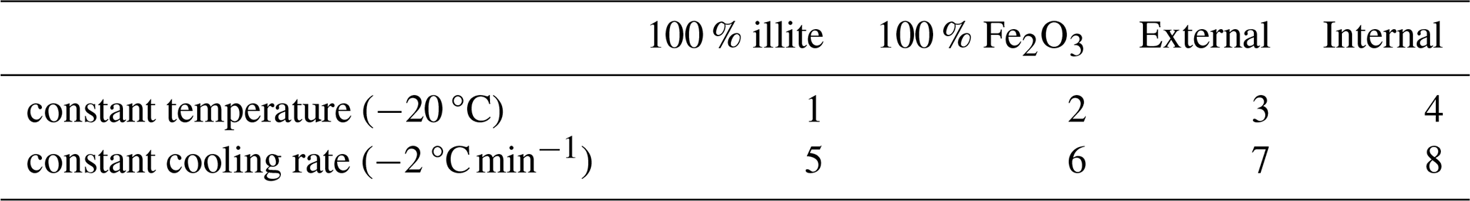
The INP populations are shown schematically in the left panel of Fig. 7. Group 1 consists solely of illite, while group 2 is exclusively made up of Fe₂O₃. In group 3, half of the particles are composed entirely of illite, and the other half entirely of Fe₂O₃, representing an external mixture. Group 4 features each particle with an even split of illite and Fe₂O₃ on its surface, constituting an internal mixture. Note that in both the external and internal mixtures, the total surface area ratio between the two species is 50:50. All four groups of INPs share the same log-normal size distribution, with a geometric mean dry diameter of 1 µm and a log-geometric standard deviation of 0.5, shown in the right panel of Fig. 7. Specifically, for the external mixture case (Group 3), we assigned identical size distributions for Fe₂O₃ and illite particles, that is, within each size bin, the particle population comprises a 50:50 ratio of pure Fe₂O₃ to pure illite particles by number concentration. It is important to note that the simulations are performed for polydisperse particles, whereas the theoretical framework in Sect. 3 is derived for monodisperse INP populations with identical particle surface areas. The implications and conditional applicability of the theory in this context are discussed in Sect. 5.3.

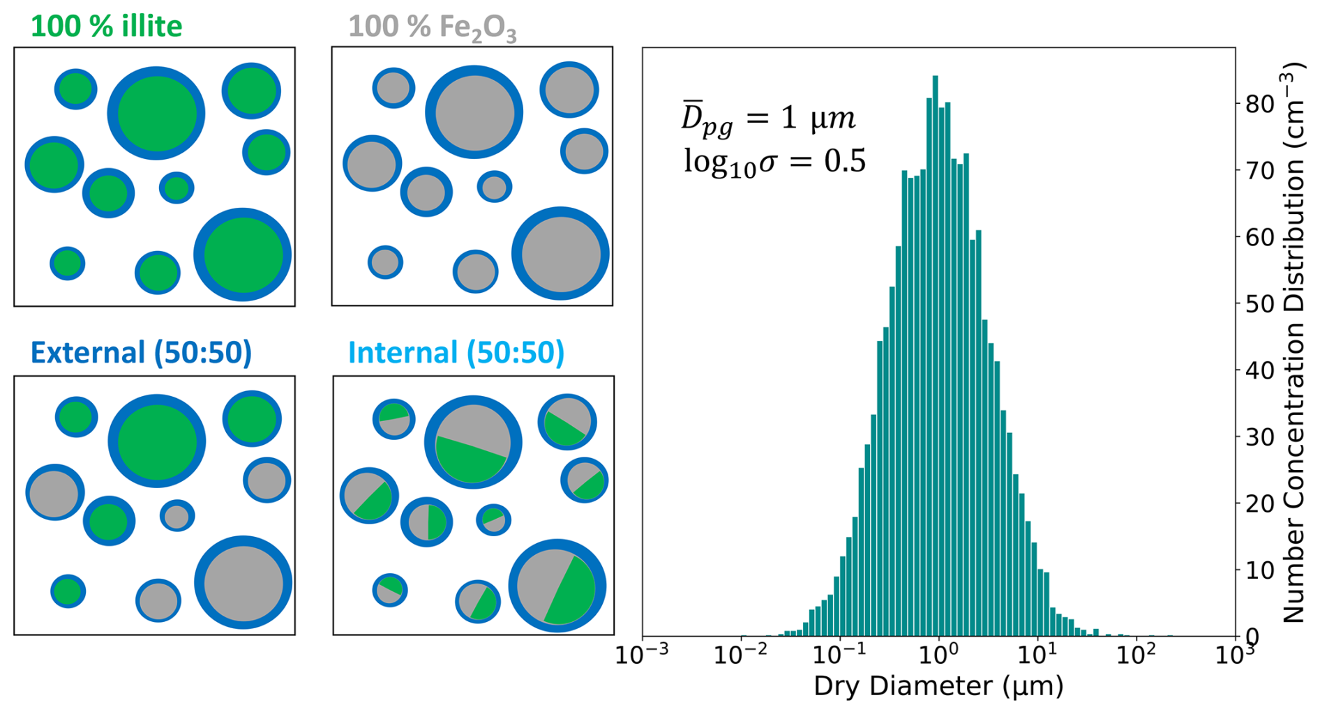
Figure 7 Model settings. Left panel: Schematic of particle mixing state for the four scenarios. The color green denotes illite, gray indicates Fe₂O₃, and blue represents the supercooled droplets that all INPs are immersed in. In both the external and internal mixtures, the total surface area ratio between the two species is 50:50. Right panel: size distribution of INPs represented by their number concentration density (cm⁻³). The geometric mean dry diameter (${\overline{D}}_{\text{pg}}$) is 1 µm and the log-geometric standard deviation (log ₁₀σ) is 0.5.

The initial condition of each simulation consists of an INP number concentration of 100 cm⁻³. All INPs were already immersed in water (one INP per droplet) and none of the INPs was frozen. We set the initial relative humidity with respect to water at 100 % to prevent evaporation of the droplets. We used 10 000 computational particles to represent the total number concentration of aerosols, with each computational particle representing 0.01 cm⁻³ aerosols sharing the same size and chemical composition.

In the isothermal experiments, the temperature was maintained at −20 °C for a duration of 10 min. Under the ccr freezing conditions, the temperature was reduced from −10 to −30 °C at a constant rate of 2 °C min⁻¹ over a period of 10 min, i.e., $T\left(t\right)=-\mathrm{10}\mathrm{°}\mathrm{C}-\mathrm{2}\mathrm{°}\mathrm{C}{\min }^{-\mathrm{1}}\cdot t$. The time interval Δt is set to 1 s. Within each interval from t to t+Δt, the temperature is assumed to remain constant at T(t). Furthermore, the simulations were limited to immersion freezing only; emissions, dilution, and coagulation were excluded from the model.

To summarize, the assumptions in the PartMC immersion freezing simulations are: (1) All INPs are spheres, the surface area is computed by the dry diameter of INP as $S_{\text{p}}=\mathit{\pi }{D}_{\mathrm{p}}^{\mathrm{2}}$. (2) Each droplet contains only one INP. (3) The volume ratio of each species of mixed particles equals their surface ratio.

5.2 Simulation Results

As an example, Fig. 8 presents the results of Case 6 (all INPs consist of Fe₂O₃ and are exposed to a ccr of 2 °C min⁻¹), displaying the simulated frozen fraction, which is confirmed by the analytical solution using Eq. (B12) in Appendix B. As the temperature drops from −10 to −30 °C, more and more INPs become activated and the frozen fraction increases (green dots).

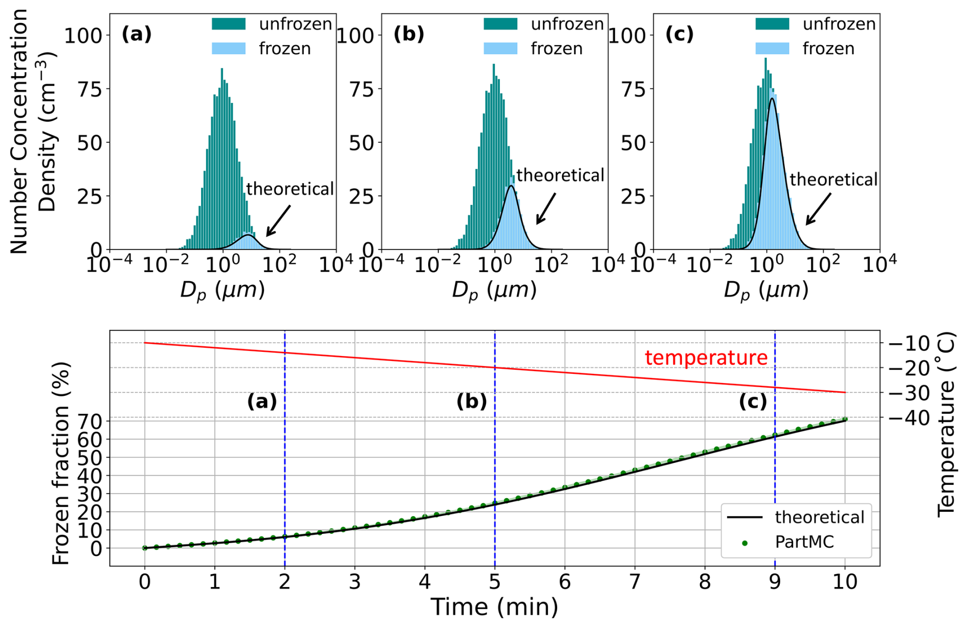
Figure 8 Comparison of model results from case 6 in Table 2 with theoretical predictions. Upper panel: Snapshots of number concentration density distribution of unfrozen (green) and frozen droplets (blue) at 2, 5, and 9 min corresponding to the blue dashed lines in the lower panel. The black solid line depicts the theoretical size distribution of activated INPs calculated using Eq. (B10). Lower panel: temperature profile (red line) and time evolution of frozen fraction from 20 realizations (green dots: the average; green shading: the minimum-maximum range), and the theoretical frozen fraction calculated using Eq. (B12) (black line).

The size distributions of activated INPs at 2, 5, and 9 min are depicted in blue in panels (a), (b), and (c) of Fig. 8, respectively. Ice crystal formation begins in droplets containing larger INPs, which are capable of activating and freezing at higher temperatures and after shorter times. Conversely, smaller INPs require more time and lower temperatures to initiate freezing, resulting in some remaining unfrozen droplets until the end. The number concentration density function for activated INPs, analytically derived from Eq. (B10) and depicted by the black solid line in subplots (a), (b), and (c), closely aligns with the histogram representing activated INPs as predicted by the PartMC model.

Figure 9 shows the simulation results for the frozen fraction for all eight cases listed in Table 2. Panel (a) illustrates Cases 1–4 conducted at a constant temperature of −20 °C, while panel (b) shows Cases 5–8, where the temperature decreased steadily from −10 to −30 °C.

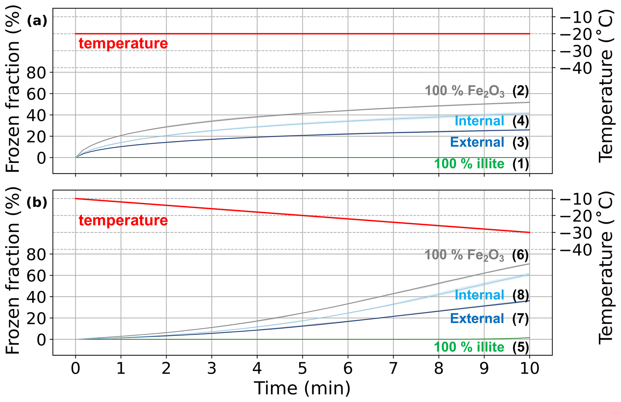
Figure 9 Simulated frozen fraction for Cases 1–8. (a) Isothermal freezing conditions, Cases 1–4. (b) ccr freezing conditions, Cases 5–8. Solid lines represent the average frozen fraction from 20 repeated simulations for each scenario, and the shaded areas denote the range between the maximum and minimum values.

In the constant-temperature cases, the ice nucleation rate for an INP remains constant, so the frozen fraction increases over time because more time allows for more nucleation events. However, the rate of this increase slows down as fewer unfrozen droplets remain available to freeze. In scenarios with a ccr, both the frozen fraction and its rate of increase increase over time. This is because the ice nucleation rate rises as the temperature continues to drop, accelerating the freezing process.

Regardless of the temperature profile, INPs composed entirely of Fe₂O₃ consistently exhibit the highest frozen fraction. Conversely, INPs made solely of illite display the lowest frozen fraction, with internal and external mixtures of these two species falling in between.

Fe₂O₃ is a highly effective freezing agent, with an ice nucleation rate coefficient of 3.5×10⁴ ${\mathrm{cm}}^{-\mathrm{2}}{\mathrm{s}}^{-\mathrm{1}}$ at −20 °C, as per the ABIFM method shown in Eq. (20). In contrast, illite exhibits a significantly lower coefficient of only 0.098 ${\mathrm{cm}}^{-\mathrm{2}}{\mathrm{s}}^{-\mathrm{1}}$ at the same temperature. This means that Fe₂O₃'s ice nucleation rate coefficient is orders of magnitude larger than that of illite. The substantial disparity in the freezing behavior of different species causes the large variations in their respective frozen fractions.

Our model results also highlight the distinctions in frozen fraction between internally and externally mixed INPs. Internally mixed INPs, comprising 50 % Fe₂O₃ and 50 % illite by surface area, exhibit a frozen fraction of 41 % in the constant temperature scenario at the end of the simulation, and 61 % in the constant cooling scenario. In contrast, externally mixed INPs, with an equal number of pure Fe₂O₃ and pure illite INPs, show a lower frozen fraction of 26 % in the constant temperature simulation, and 36 % in the simulation with decreasing temperature. Even though the total surface area of the INPs is the same for both species, and the cooling condition is consistent across both groups with different mixing states, a significant disparity in the frozen fraction is observed between internal and external mixtures. These results are consistent with the main conclusion in Sect. 3 and further illustrate, in a particle-resolved modeling framework, how mixing state influences the quantity of ice formation.

Figure 10 presents another view of the comparison of frozen fraction results between analytical calculations and PartMC simulations for all eight cases listed in Table 2. Each point represents the frozen fraction at one simulation time step, so results from all time steps are included. Generally, the model's results closely align with the theoretical values, with an RMSE of less than 1 % and a correlation coefficient exceeding 0.9999, except for Case 1. The discrepancy in Case 1 arises from the discreteness of computational particles in the PartMC simulation. Because the frozen fraction in this case is extremely low, on the order of 10⁻³ %, accurately resolving it with only 10 000 computational particles becomes challenging. An order-of-magnitude estimate of the computational particle number required to suppress sampling noise is provided in Appendix I. That estimate suggests that resolving frozen fractions at the level of Case 1 with a relative uncertainty of about 10 % would require on the order of 10⁷–10⁸ computational particles. The results in this section demonstrate the implementation of the immersion freezing algorithm for multi-species INPs in PartMC, verified against the analytical solution.

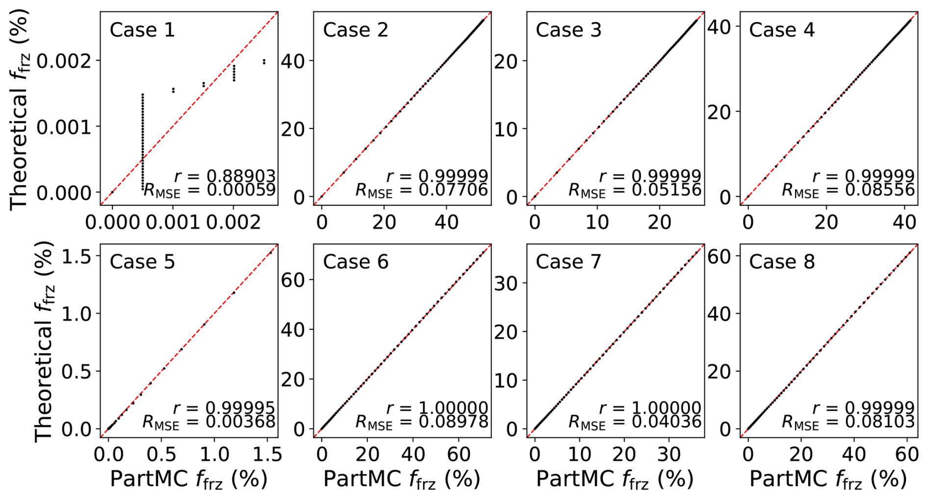
Figure 10 Comparison of frozen fraction between analytical calculations and PartMC simulations for the eight cases listed in Table 2 (Cases 1–8). The PartMC results are obtained from an ensemble mean of 20 repeated simulations. Each panel corresponds to one case, and each point represents the frozen fraction at one simulation time step (all time steps are included). The red dashed line indicates the 1:1 relationship between the simulated and theoretical values.

5.3 Immersion freezing simulations for INPs with intermediate mixing state

According to Theorem 1, for monodisperse particles, the frozen fractions of internally-mixed and externally-mixed INPs define the upper and lower bounds, and any intermediate mixing state will result in frozen fractions in between these two extremes. In this section, we will use PartMC to confirm this conclusion quantitatively, and discuss its applicability to polydisperse particles.

We use the χ index based on surface area as a metric to quantify the mixing state of INPs. Originally proposed by Riemer and West (2013), the χ index was designed to characterize the mixing state of an aerosol population, ranging from internally to externally mixed, based on species' mass fractions. In our study, we modify this definition by replacing mass fraction with surface area fraction for each species to better account for the ice nucleation properties of INPs (see details in Appendix G). Figure 11 illustrates the aerosol mixing states as characterized by the χ index (with respect to surface), where χ=0 % signifies an external mixture and χ=100 % indicates an internal mixture. Values of χ ranging between 0 % and 100 % denote intermediate mixtures, representing a continuum between external and internal mixing states. This conceptual framework is essential for comprehending the diverse nature of atmospheric aerosols and their varying properties.

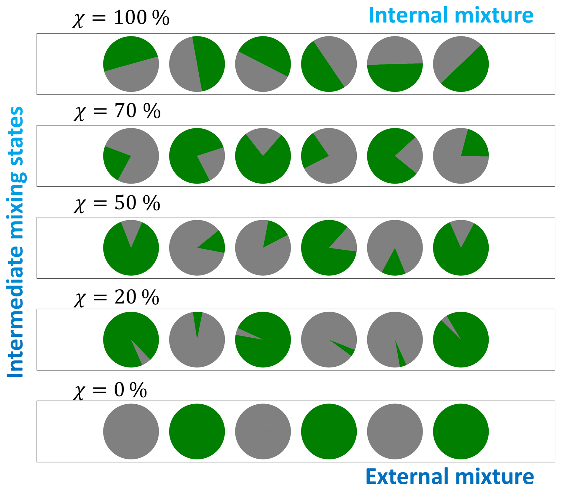
Figure 11 Schematic diagram of different aerosol mixing states described by various χ indices, where green and gray represent two different aerosol species.

Although Theorem 1 is formally derived for a monodisperse INP population, it can be reasonably extended to polydisperse populations, provided that the surface area ratio of species is specified within each size bin. When this condition is met, the polydisperse population can be treated as a collection of monodisperse subpopulations, allowing Theorem 1 to be applied to each bin individually. Under these assumptions, the internal mixture remains the most efficient one – since every particle within each bin exhibits the highest available ice nucleation efficiency – while the external mixture is the least efficient, as fewer particles possess the highly active nucleating surface. Figure 12 illustrates an applicability example of Theorem 1. The polydisperse INP populations shown in panels (a)–(c) share the same size distribution and an identical total surface area ratio of 50:50 between species A (gray) and B (green). Panel (a) shows an internal mixture, while panels (b) and (c) represent external mixtures. Theorem 1 is applicable to the efficiency comparison between panels (a) and (b), since each bin corresponding to the same INP size has the same species surface area ratio (50:50) in both cases. However, Theorem 1 is not applicable to the comparison between panels (a) and (c), because the species surface area ratio within individual bins differs. For example, while the first bin in panel (a) has a 50:50 ratio, it is 100:0 in panel (c). Similarly, other bins exhibit inconsistent ratios between panels (a) and (c), despite having the same total surface area ratio (50:50) when aggregated across all bins. Following PartMC simulation results illustrate how the frozen fraction varies with the mixing state index (χ) for a polydisperse INP population, while maintaining a 50:50 surface area ratio of Fe₂O₃ and illite particles in each bin.

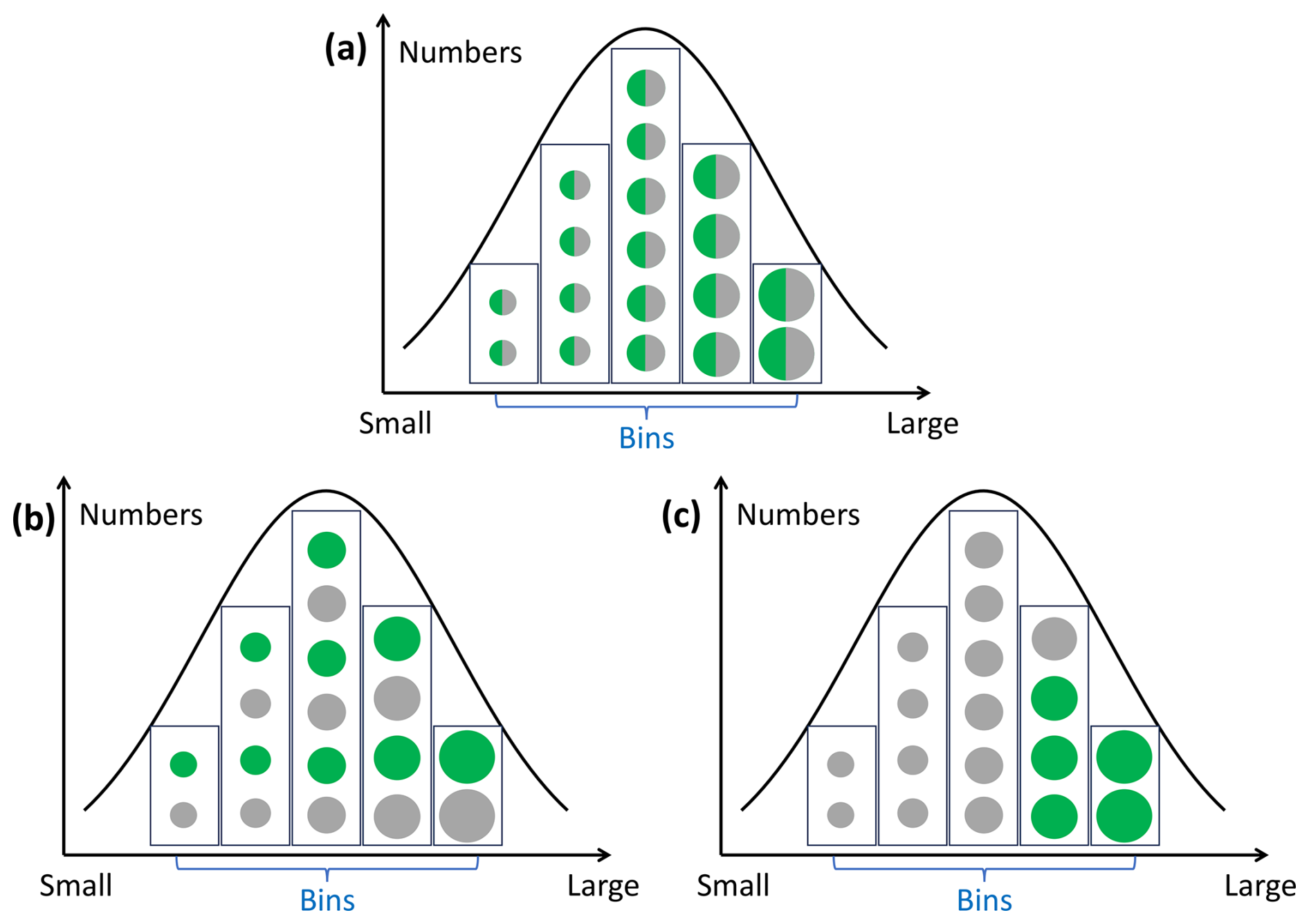
Figure 12 Schematic figure demonstrating the applicability of Theorem 1 to polydisperse INPs. Panels (a)–(c) depict the mixing states within 5-bin samples, where particles share the same size within each bin but differ in size across bins. Panel (a) represents an internal mixture, while panels (b) and (c) represent external mixtures. All three panels share the same size distribution, and the total surface area ratio between species A (gray) and B (green) is 50:50. In panels (a) and (b), the surface area ratio between species A and B is also 50:50 within each bin; however, this ratio does not hold for the INPs shown in panel (c).

We initialized the model with a series of INP populations characterized by varying intermediate mixing states, with the χ value for INPs in each bin were set to 10 %, 20 %, 30 %, 40 %, 50 %, 60 %, 70 %, 80 %, and 90 % for each respective simulation case respectively. All populations shared the same size distribution, as illustrated in the right panel of Fig. 7, and had the same number concentration of 100 cm⁻³. Each INP population was divided into 100 size bins, within which the total surface ratio is composed of 50 % Fe₂O₃ and 50 % illite. The method we used to construct an intermediate mixing states with a specific χ in each bin is detailed in Appendix H.

Two types of simulation were conducted for each of the nine INP populations with intermediate mixing states. One is the isothermal scenario, with a constant temperature of −20 °C for 10 min, the same as Cases 1–4; the other involves a ccr of −2 °C min⁻¹ over 10 min, the same as Cases 5–8. All model assumptions are the same as those in Sect. 5.1, so that the isothermal simulations for intermediate mixing state INPs are comparable to Cases 3 (external mixture) and 4 (internal mixture), and ccr simulations are comparable to Cases 7 (external mixture) and 8 (internal mixture).

The time series of simulated frozen fraction for all intermediate mixing state cases are shown in Fig. 13, with the upper panel representing the isothermal experiments and the lower panel representing the constant cooling experiments. Cases 3 and 4 are also shown in the upper panel as references for external and internal mixtures in the constant temperature scenario, marked as χ=0 % and χ=100 %, respectively. Similarly, results from Cases 7 and 8 are shown in the lower panel as references for external and internal mixtures in the constant cooling scenario. Regardless of whether the scenario involves constant temperature or ccr, the frozen fractions of intermediate-mixed INPs fall between those of internally and externally mixed INPs, ordered according to the χ value.

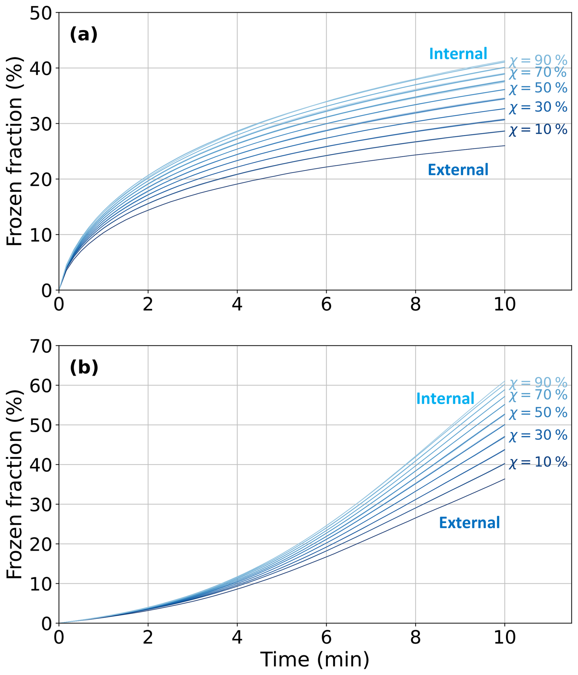
Figure 13 Time series of frozen fraction for immersed INPs with specific mixing state under (a) isothermal freezing conditions with −20 °C and (b) ccr freezing conditions from −10 to −30 °C within 10 min. Each line corresponds to a specific mixing state of INPs, identified by varying values of the mixing state index χ, which ranges from 0 % (purely external mixture) to 100 % (purely internal mixture).

The frozen fractions of the internal and external mixtures set the upper and lower bounds for the frozen fraction of the intermediate mixing state, respectively. This confirms the argument made in Theorem 1. In cases where the mixing state is unknown, assuming the INP population is in an internal mixture during simulations would lead to the largest error in the frozen fraction estimation if the actual state is an external mixture. All other intermediate mixing states would result in smaller overprediction. The uncertainty mentioned here can be quantified by the sensitivity defined by Eq. (10), which describes the maximum range of the “mixing state effect” on the frozen fraction.

6 Discussion and Conclusion

This study developed a theoretical and modeling framework to quantify how aerosol mixing state influences immersion freezing. We derived analytical expressions linking the frozen fraction to particle composition and mixing state, showing that internally mixed populations yield systematically higher ice fractions than externally mixed ones under identical environmental conditions.

We implemented a multi-species immersion freezing scheme in the particle-resolved model PartMC, using the ABIFM parameterization for heterogeneous nucleation rates. To improve computational efficiency, we incorporated a Binned Tau-Leaping algorithm, which achieved nearly an order-of-magnitude speedup while preserving accuracy. Simulations validated the theoretical results and quantified the influence of particle size, species type, and surface coverage on freezing behavior.

It is important to note that this study adopts the time-dependent description of immersion freezing based on classical nucleation theory (CNT) in its numerical implementation. While there is ongoing debate in the community regarding the relative merits of the CNT-based (stochastic) and singular (threshold-based) approaches, our implementation focuses on CNT to avoid additional complexity and to build on a physical framework. Recent comparative evaluations, both in context of laboratory studies (e.g., Szakáll et al., 2021) and model development (e.g., Arabas et al., 2025), suggest that CNT offers greater robustness, also in light of capturing multiple-component aerosol materials. In the singular/INAS framework, the quantity Φ in our notation can be interpreted as analogous to the surface site density n_S, which characterizes the ice-nucleating activity of a given species. Specifically, under a given temperature profile T(τ), we have $\mathrm{\Phi }\left(t\right)=n_{\mathrm{S}}\left({min}_{\mathit{\tau }\in [\mathrm{0},t]}T\right(\mathit{\tau }\left)\right)$. Although CNT and INAS differ in their underlying physical interpretations, this correspondence implies that Theorem 1 and the sensitivity analysis in Sect. 3 remain applicable within the INAS framework. For a given species under the same T(τ), ABIFM/CNT and INAS may assign different numerical values to Φ, but the structural dependence on surface activity is preserved. Accordingly, if Φ_A and Φ_B are interpreted as the corresponding n_S values for species A and B, the sensitivity patterns shown in Figs. 3–5 remain valid, although the species labels in Fig. 3 would differ because those examples are based on ABIFM. This interpretation is conceptually related to the “soccer-ball” model of Niedermeier et al. (2011, 2014), in which particle surfaces are divided into stochastic surface patches with contact angles drawn from a prescribed distribution. In that framework, small n_site yields stronger particle-to-particle variability in nucleating properties, whereas very large n_site makes particles more similar in their site-property distributions. Their results showed that such surface heterogeneity can make a fundamentally stochastic freezing process appear nearly singular at the population level. Our study differs in that we focus not on heterogeneity in site-specific contact angles, but on heterogeneity in the distribution of chemical species across particles for a fixed bulk composition and size distribution. Both approaches nevertheless point to the same broader conclusion: the distribution of ice-nucleation-relevant properties within and across particles is a key control on the frozen fraction.

The PartMC model calculates the surface area of INPs based on their dry diameter, assuming that the particles are spherical. However, real atmospheric aerosols exhibit a wide range of shapes and surface textures (e.g., Dick et al., 1998; Chou et al., 2008; Adachi et al., 2010; Valsan et al., 2016; Conny and Buseck, 2024), which challenges the validity of this simplifying assumption. Even particles that appear approximately spherical may have complex surface features – such as folds, pits, or protrusions – that lead to underestimation of their true surface area when diameter alone is used. A related simplification arises in representing particle's morphology in the particle-resolved simulations. In the current PartMC implementation, species composition is tracked in terms of mass, while particle morphology and surface exposure of individual species are not explicitly resolved. In the absence of such information, we assume that the surface area fraction of each species is proportional to its volume (or mass) fraction within a particle. This assumption provides a practical way to prescribe surface area partitioning among species but may not hold for particles with complex internal structures or coating morphologies. Accurately representing the ice-nucleating potential of such particles in atmospheric models therefore requires a more realistic estimation of surface area (Alpert and Knopf, 2016; Knopf et al., 2020). One approach is to compute a surface-area-equivalent diameter, which can then be used as model input to reduce biases in ice nucleation predictions arising from the spherical assumption and from simplified representations of species surface exposure.

The current algorithm is designed to simulate immersion freezing in particles composed entirely of insoluble species, such as illite, kaolinite, Fe₂O₃, and Al₂O₃. Its applicability becomes limited, however, when particles contain soluble components, requiring a more nuanced treatment. If a particle is fully soluble, it dissolves completely upon droplet formation, leaving no solid surface to initiate immersion freezing. In such cases, only homogeneous nucleation is expected. For mixed particles containing both soluble and insoluble components, the soluble fraction dissolves into the droplet, altering its water activity a_w, which then deviates from that of pure water (a_w=1; see Eq. 20). This shift must be quantified based on the ratio of soluble material to water volume (Berkemeier et al., 2016; Charnawskas et al., 2017; Knopf et al., 2018). The remaining insoluble core can still act as an INP, but its surface area may differ significantly from that of the original particle, requiring recalculation based on the volume of the insoluble fraction. Additionally, certain species – such as 1-nonadecanol – can act as surfactants, forming films on the droplet surface and increasing the effective ice-nucleating area. To account for these complexities, the model will need to be expanded in future work to include the effects of solubility, water activity, and surfactant behavior on ice nucleation.

The theoretical investigation revealed that the fundamental difference in the unfrozen fraction between internally and externally mixed INPs is mathematically equivalent to the difference between the surface area-weighted geometric and arithmetic means of the frozen fractions that each species would exhibit if it individually dominated the INPs. Under identical environmental conditions, internally mixed monodisperse INP populations exhibit the highest frozen fraction, whereas externally mixed populations exhibit the lowest, with all other intermediate mixing states falling within this range. A systematic analysis of the sensitivity map reveals that in INP populations composed of multiple species, the impact of the mixing state becomes significant when there is a species with very high freezing efficiency that differs markedly from the other species, especially when this species occupies only a small fraction of the total surface area. These insights highlight the profound impact of the mixing state on ice formation processes, particularly when INPs comprise materials with notably diverse freezing characteristics. This research emphasizes the importance of considering the mixing state of INPs to enhance the precision of ice nucleation predictions in mixed-phase cloud environments.

The particle-resolved simulation results of immersion freezing using the PartMC model demonstrated a robust representation of the immersion freezing process, well-supported by theoretical predictions. Further analysis highlighted the superiority of the Binned Tau-leaping algorithm over the naive algorithm, both in terms of efficiency and precision, for predicting INPs' freezing behavior. The simulated frozen fraction results showed excellent agreement with theoretical calculations, providing successful verification of the frozen fraction equation proposed in this study. Significant distinctions were observed in PartMC simulations between single-species and multi-species INPs, as well as between INPs in internal and external mixtures. Simulations of intermediate mixed INPs confirmed that, for monodisperse INP populations (or INPs within the same bin), internal and external mixtures represent two extreme cases that define the upper and lower bounds for other mixing states. This finding is consistent with the theoretical conclusions presented earlier. Furthermore, the results quantitatively demonstrated that the frozen fraction increases with the χ index of two-species INPs, providing an illustration of how the mixing state influences the frozen fraction of mixed INPs.

With the advancement of single-particle analytical techniques capable of identifying surface chemical composition (e.g., Knopf et al., 2014; Laskin et al., 2016; Knopf et al., 2018, 2021; Lata et al., 2021; Alpert et al., 2022; Knopf et al., 2023; Xue et al., 2024), the model developed here is well suited to incorporate such detailed particle-level information, enabling more accurate predictions of immersion freezing and, ultimately, improved estimates of ice crystal number concentrations.

Appendix A: Derivation details

A1 Derivation of the single-particle freezing probability: Equation (2)

The immersion freezing probability of supercooled droplet can be described by the Poisson model (Pruppacher and Klett, 1996; Koop et al., 1997), the probability of N ice nucleation triggering events occurring within time Δt is

$$\begin{array}{}\text{(A1)}& P(N,\mathrm{\Delta }t)={\displaystyle \frac{\mathrm{1}}{N\mathrm{!}}}\cdot (\mathit{\lambda }\mathrm{\Delta }t{)}^N\cdot e^{-\mathit{\lambda }\mathrm{\Delta }t},\end{array}$$

where λ represents the ice nucleation rate (unit: s⁻¹). Therefore, the probability of N≥1 events occurring during Δt is

$$\begin{array}{}\text{(A2)}& \begin{array}{rl}{P}_{\text{frz}}\left(\mathrm{\Delta }t\right)& =P(N\ge \mathrm{1},\mathrm{\Delta }t)=\mathrm{1}-P(N=\mathrm{0},\mathrm{\Delta }t)\\ & =\mathrm{1}-e^{-\mathit{\lambda }\mathrm{\Delta }t},\end{array}\end{array}$$

which is also the freezing probability of a droplet containing the particle within the time interval Δt, shown in Eq. (1).

Let us divide the total cooling time, denoted as t, into h discrete time intervals Δt. Thus, we have

$$\begin{array}{}\text{(A3)}& t=h\cdot \mathrm{\Delta }t.\end{array}$$

If a droplet remains unfrozen until the time t, it was unfrozen throughout each time interval. On the other hand, if it freezes at any time point, it will remain frozen for the remainder of the calculation, as the melting process is not considered. Here, we regard the ice nucleation rate as a function of time, denoted by λ(τ), and the probability of a droplet remaining unfrozen from t₁ to t₂ is denoted by P_unf(t₁,t₂). The probability of a droplet remaining unfrozen from 0 to t, denoted by P_unf(0,t), can be formulated as

$$\begin{array}{ll}{\displaystyle }{P}_{\text{unf}}(\mathrm{0},t)=& {\displaystyle }{P}_{\text{unf}}(\mathrm{0},\mathrm{\Delta }t)\cdot P_{\text{unf}}(\mathrm{\Delta }t,\mathrm{2}\mathrm{\Delta }t)\\ {\displaystyle }& {\displaystyle }\cdot P_{\text{unf}}(\mathrm{2}\mathrm{\Delta }t,\mathrm{3}\mathrm{\Delta }t)\cdot \\ \text{(A4)}& {\displaystyle }& {\displaystyle }\mathrm{\dots }\cdot P_{\text{unf}}\left(\right(h-\mathrm{1})\mathrm{\Delta }t,h\mathrm{\Delta }t){\displaystyle }=& {\displaystyle }\exp \left[-\mathit{\lambda }\left(\mathrm{0}\right)\cdot \mathrm{\Delta }t\right]\cdot \exp \left[-\mathit{\lambda }\left(\mathrm{\Delta }t\right)\cdot \mathrm{\Delta }t\right]\\ {\displaystyle }& {\displaystyle }\cdot \exp \left[-\mathit{\lambda }\left(\mathrm{2}\mathrm{\Delta }t\right)\cdot \mathrm{\Delta }t\right]\cdot \\ \text{(A5)}& {\displaystyle }& {\displaystyle }\mathrm{\dots }\cdot \exp \left[-\mathit{\lambda }\left(\right(h-\mathrm{1}\left)\mathrm{\Delta }t\right)\cdot \mathrm{\Delta }t\right]\text{(A6)}& {\displaystyle }=& {\displaystyle }{e}^{-\left[{\sum }_{k=\mathrm{0}}^{h-\mathrm{1}}\mathit{\lambda }\left(k\mathrm{\Delta }t\right)\cdot \mathrm{\Delta }t\right]},\end{array}$$

where h is the number of time intervals dividing the time period from 0 to t. Considering the limits Δt→0 and h→∞, the unfrozen probability P_unf(0,t) is given by the time integration of λ:

$$\begin{array}{}\text{(A7)}& \begin{array}{rl}{P}_{\text{unf}}(\mathrm{0},t)& =\underset{\mathrm{\Delta }t\to \mathrm{0},h\to +\mathrm{\infty }}{lim}{e}^{-\left[{\sum }_{k=\mathrm{0}}^{h-\mathrm{1}}\mathit{\lambda }\left(k\mathrm{\Delta }t\right)\mathrm{\Delta }t\right]}\\ & =e^{-{\int }_{\mathrm{0}}^t\mathit{\lambda }\left(\mathit{\tau }\right)\mathrm{d}\mathit{\tau }}.\end{array}\end{array}$$

Therefore, the probability of freezing from t=0 to t is

$$\begin{array}{}\text{(A8)}& P_{\text{frz}}(\mathrm{0},t)=\mathrm{1}-e^{-{\int }_{\mathrm{0}}^t\mathit{\lambda }\left(\mathit{\tau }\right)\mathrm{d}\mathit{\tau }},\end{array}$$

where P_frz(0,t) is, for simplicity, denoted as P_frz(t) in Eq. (2).

A2 Derivation of the frozen fraction equation for monodisperse INPs with external mixture: Equation (13)

An externally mixed monodisperse INP population can be conceptualized as a set of distinct species, each represented by particles composed of a single species. Let us define w_i as the ratio of the total surface area covered by the ith species relative to the total surface area across all INPs

$$\begin{array}{}\text{(A9)}& w_i={\displaystyle \frac{{\sum }_{j=\mathrm{1}}^{N_{\mathrm{p}}}{S}_j^{\left(i\right)}}{{\sum }_{j=\mathrm{1}}^{N_{\mathrm{p}}}{S}_{{\mathrm{p}}_j}}},\end{array}$$

where, $S_{{\mathrm{p}}_j}$ is the immersed surface area of the jth particle, and $S_j^{\left(i\right)}$ denotes the area covered by the ith species on the jth particle. For a monodisperse INP population, all INPs are assumed to have the same immersed surface area, $S_{{\mathrm{p}}_j}=S_{\mathrm{p}}$. As each INP is covered by a single species, these ratios are determined purely by the numbers of INPs within each mode. Thus, the total surface area ratio of ith species equals the fraction of INPs that covered by the ith species:

$$\begin{array}{}\text{(A10)}& w_i={\displaystyle \frac{{\sum }_{j=\mathrm{1}}^{N_{\mathrm{p}}}{S}_j^{\left(i\right)}}{{\sum }_{j=\mathrm{1}}^{N_{\mathrm{p}}}{S}_{{\mathrm{p}}_j}}}={\displaystyle \frac{N_{\mathrm{p}}^{\left(i\right)}{S}_{\mathrm{p}}}{N_{\mathrm{p}}{S}_{\mathrm{p}}}}={\displaystyle \frac{N_{\mathrm{p}}^{\left(i\right)}}{N_{\mathrm{p}}}}\end{array}$$

where $N_{\mathrm{p}}^{\left(i\right)}$ is the total number of the ith mode particle. The overall number of unfrozen particles is the sum of the number of unfrozen particles from all modes

$$\begin{array}{}\text{(A11)}& N_{\text{unf}}=\sum _{i=\mathrm{1}}^{N_{\mathrm{s}}}{N}_{\text{unf}}^{\left(i\right)},\end{array}$$

where $N_{\text{unf}}^{\left(i\right)}$ is the number of unfrozen particles for the mode consisting of INPs covered by the ith species. Following the definition of unfrozen fraction, and incorporating Eqs. (A10) and (A11), the unfrozen fraction is given by

$$\begin{array}{}\text{(A12)}& \begin{array}{rl}{f}_{\text{unf}}^{\text{(ext)}}& ={\displaystyle \frac{N_{\text{unf}}}{N_{\mathrm{p}}}}={\displaystyle \frac{\mathrm{1}}{N_{\mathrm{p}}}}\cdot \sum _{i=\mathrm{1}}^{N_{\mathrm{s}}}{N}_{\text{unf}}^{\left(i\right)}={\displaystyle \frac{\mathrm{1}}{N_{\mathrm{p}}}}\cdot \sum _{i=\mathrm{1}}^{N_{\mathrm{s}}}{N}_{\mathrm{p}}^{\left(i\right)}\cdot f_{\text{unf}}^{\left(i\right)}\\ & =\sum _{i=\mathrm{1}}^{N_{\mathrm{s}}}{w}_i\cdot f_{\text{unf}}^{\left(i\right)},\end{array}\end{array}$$

where $f_{\text{unf}}^{\left(i\right)}$ denotes the unfrozen fraction of INPs in the ith mode. The Eq. (A12) is the same as Eq. (12) in the Sect. 3.1. Since $f_{\text{frz}}^{\text{(ext)}}=\mathrm{1}-f_{\text{unf}}^{\text{(ext)}}$ and $f_{\text{frz}}^{\left(i\right)}=\mathrm{1}-f_{\text{unf}}^{\left(i\right)}$, there is

$$\begin{array}{}\text{(A13)}& f_{\text{frz}}^{\text{(ext)}}=\mathrm{1}-\sum _{i=\mathrm{1}}^{N_{\mathrm{s}}}{w}_i\cdot f_{\text{unf}}^{\left(i\right)}=\mathrm{1}-\sum _{i=\mathrm{1}}^{N_{\mathrm{s}}}{w}_i\cdot (\mathrm{1}-f_{\text{frz}}^{\left(i\right)}),\end{array}$$

which is the Eq. (13) shown in Sect. 3.1.

A3 Derivation of the frozen fraction equation for monodisperse INPs with internal mixture: Equation (15)

For an INP immersed in a supercooled droplet, composed of multiple species, let the total number of species be N_s, with $w_i=S_i/S$ denoting the surface covering ratio of the ith species, where S_i is the area covered by the ith species and S is the total surface area of the INP. Assuming the temperature remains below 0 °C, based on Eq. (9), the probability of the droplet remaining unfrozen after time t is

$$\begin{array}{}\text{(A14)}& P_{\text{unf}}\left(t\right)=\mathrm{1}-P_{\text{frz}}\left(t\right)=e^{-S_{\mathrm{p}}\cdot {\sum }_{i=\mathrm{1}}^{N_{\mathrm{s}}}{w}_i{\mathrm{\Phi }}_i\left(t\right)}.\end{array}$$

Denoting $P_{\text{unf}}^{\left(i\right)}=e^{-S_{\mathrm{p}}\cdot {\mathrm{\Phi }}_i\left(t\right)}$ the droplet's unfrozen probability for an INP of the same size but with its surface 100 % covered by the ith species, we obtain

$$\begin{array}{}\text{(A15)}& P_{\text{unf}}^{\left(i\right)}=\mathrm{1}-P_{\text{frz}}^{\left(i\right)}=e^{-S_{\mathrm{p}}\cdot {\mathrm{\Phi }}_i\left(t\right)},\forall i\in \left[\mathrm{1},N_{\mathrm{s}}\right].\end{array}$$

Combining Eq. (A14) and Eq. (A15) gives:

$$\begin{array}{}\text{(A16)}& \begin{array}{rl}{P}_{\text{unf}}& =\mathrm{1}-P_{\text{frz}}=e^{-S_{\mathrm{p}}\cdot {\sum }_{i=\mathrm{1}}^{N_{\mathrm{s}}}{w}_i\cdot {\mathrm{\Phi }}_i\left(t\right)}\\ & =\prod _{i=\mathrm{1}}^{N_{\mathrm{s}}}(e^{-S_{\mathrm{p}}\cdot {\mathrm{\Phi }}_i\left(t\right)}{)}^{w_i}=\prod _{i=\mathrm{1}}^{N_{\mathrm{s}}}(P_{\text{unf}}^{\left(i\right)}{)}^{w_i}.\end{array}\end{array}$$

For an internally mixed population of monodisperse INPs, each INP has the same size and the ratio of surface covered by each species. Therefore, the freezing probabilities are the same for each INP (same for the unfrozen probabilities). Based on the Law of Large Numbers, the unfrozen fraction equals the unfrozen probability of each droplet,

$$\begin{array}{}\text{(A17)}& f_{\text{unf}}=P_{\text{unf}}.\end{array}$$

The same also applies for monodisperse INPs covered by a single species i:

$$\begin{array}{}\text{(A18)}& f_{\text{unf}}^{\left(i\right)}=P_{\text{unf}}^{\left(i\right)},\forall i\in \left[\mathrm{1},N_{\mathrm{s}}\right].\end{array}$$

Substituting Eqs. (A17) and (A18) to Eq. (A16), we have:

$$\begin{array}{}\text{(A19)}& f_{\text{unf}}^{\text{(int)}}=\prod _{i=\mathrm{1}}^{N_{\mathrm{s}}}{\left(f_{\text{unf}}^{\left(i\right)}\right)}^{w_i},\end{array}$$

the same as Eq. (14) in Sect. 3.1. Since $f_{\text{frz}}^{\text{(int)}}=\mathrm{1}-f_{\text{unf}}^{\text{(int)}}$ and $f_{\text{frz}}^{\left(i\right)}=\mathrm{1}-f_{\text{unf}}^{\left(i\right)}$, there is

$$\begin{array}{}\text{(A20)}& f_{\text{frz}}^{\text{(int)}}=\mathrm{1}-\prod _{i=\mathrm{1}}^{N_{\mathrm{s}}}{\left(\mathrm{1}-f_{\text{frz}}^{\left(i\right)}\right)}^{w_i},\end{array}$$

which is equal to Eq. (15) shown in Sect. 3.1.

Appendix B: Ice number concentration for single-mode polydisperse INP population

Equation (9) outlines the freezing probability for an individual droplet. In this appendix, we derive equations that describe the ice crystal number concentration and the frozen fraction for a collection of single-mode INPs immersed in supercooled droplets, subject to a specific temperature profile. A “mode” in this context refers to a group of particles whose sizes follow a specified distribution, and all particles within the mode have the same composition.

Assuming that each droplet contains only one INP, and each INP is spherical. The surface area of each INP, S_p, can be calculated by

$$\begin{array}{}\text{(B1)}& S_{\mathrm{p}}=\mathit{\pi }{D}_{\mathrm{p}}^{\mathrm{2}}.\end{array}$$

It is also assumed that no ice formation occurs at the initial time. Additionally, we maintain the temperature below 0 °C throughout the simulation to prevent melting. Moreover, we assume that all INPs contain the same species types and their surface coverage for all INPs is identical (i.e., single-species and internally mixed INPs with respect to surface), in order to satisfy the definition of the single-mode particles.

For monodisperse INPs, given that the size and surface fractions of species are uniform across all INPs, all droplets have the same freezing probability at any given time. According to the Law of Large Numbers, the expected value of the frozen fraction is equivalent to the freezing probability of each individual droplet

$$\begin{array}{}\text{(B2)}& f_{\text{frz}}\left(t\right)\equiv P_{\text{frz}}\left(t\right).\end{array}$$

Consequently, the ice number concentration can be expressed as

$$\begin{array}{}\text{(B3)}& {\stackrel{\mathrm{̃}}{N}}_{\text{frz}}\left(t\right)={\stackrel{\mathrm{̃}}{N}}_{\mathrm{t}}\cdot f_{\text{frz}}\left(t\right)={\stackrel{\mathrm{̃}}{N}}_{\mathrm{t}}\cdot P_{\text{frz}}\left(t\right).\end{array}$$

In the case of polydisperse INPs, the freezing probability of each droplet varies depending on the diameter of the contained INP, denoted as P_frz(t,D_p). Combining Eq. (9) and Eq. (B1), we have

$$\begin{array}{}\text{(B4)}& P_{\text{frz}}(t,D_{\mathrm{p}})=\mathrm{1}-e^{-\mathit{\pi }{D}_{\mathrm{p}}^{\mathrm{2}}\cdot \overline{\mathrm{\Phi }}\left(t\right)}.\end{array}$$

where $\overline{\mathrm{\Phi }}\left(t\right)$ represents the time integrated surface area-weighted mean of the ice nucleation rate coefficient, given by

$$\begin{array}{}\text{(B5)}& \begin{array}{rl}\overline{\mathrm{\Phi }}\left(t\right)& ={\int }_{\mathrm{0}}^t{\overline{J}}_{\text{het}}\left(T\right(\mathit{\tau }\left)\right)\mathrm{d}\mathit{\tau }={\int }_{\mathrm{0}}^t\sum _{i=\mathrm{1}}^{N_{\mathrm{s}}}{w}_i\cdot J_{\text{het}}^{\left(i\right)}\left(T\right(\mathit{\tau }\left)\right)\mathrm{d}\mathit{\tau }\\ & =\sum _{i=\mathrm{1}}^{N_{\mathrm{s}}}{w}_i\cdot \left({\int }_{\mathrm{0}}^t{J}_{\text{het}}^{\left(i\right)}\left(T\right(\mathit{\tau }\left)\right)\mathrm{d}\mathit{\tau }\right)=\sum _{i=\mathrm{1}}^{N_{\mathrm{s}}}{w}_i\cdot {\mathrm{\Phi }}_i\left(t\right),\end{array}\end{array}$$

Herein, we define the size distribution density function n_N(ln D_p) to represent the size distribution of INPs. Analogous to the Eq. (B3), the size distribution density function for “activated” INPs (those that cause the freezing of droplet in which they are immersed) can be expressed as

$$\begin{array}{}\text{(B6)}& \begin{array}{rl}{n}_{\text{frz}}(t,\ln D_{\mathrm{p}})& =n_{\mathrm{N}}\left(\ln D_{\mathrm{p}}\right)\cdot P_{\text{frz}}(t,D_{\mathrm{p}})\\ & =n_{\mathrm{N}}\left(\ln D_{\mathrm{p}}\right)\cdot (\mathrm{1}-e^{-\mathit{\pi }{D}_{\mathrm{p}}^{\mathrm{2}}\cdot \overline{\mathrm{\Phi }}\left(t\right)}).\end{array}\end{array}$$

Consequently, the ice crystal number concentration, which is the aggregate of the numbers of “activated” INPs across all sizes, can be calculated as follows

$$\begin{array}{}\text{(B7)}& \begin{array}{rl}{\stackrel{\mathrm{̃}}{N}}_{\text{frz}}\left(t\right)& ={\int }_{-\mathrm{\infty }}^{+\mathrm{\infty }}{n}_{\text{frz}}(t,\ln D_{\mathrm{p}})\cdot \mathrm{d}\ln D_{\mathrm{p}}\\ & ={\stackrel{\mathrm{̃}}{N}}_{\mathrm{t}}-{\int }_{-\mathrm{\infty }}^{+\mathrm{\infty }}{n}_{\mathrm{N}}(t,\ln D_{\mathrm{p}})\cdot e^{-\mathit{\pi }{D}_{\mathrm{p}}^{\mathrm{2}}\cdot \overline{\mathrm{\Phi }}\left(t\right)}\mathrm{d}\ln D_{\mathrm{p}},\end{array}\end{array}$$

and the frozen fraction can be derived by

$$\begin{array}{}\text{(B8)}& \begin{array}{rl}{f}_{\text{frz}}& ={\stackrel{\mathrm{̃}}{N}}_{\text{frz}}\left(t\right)/{\stackrel{\mathrm{̃}}{N}}_{\mathrm{t}}\\ & =\mathrm{1}-{\displaystyle \frac{\mathrm{1}}{{\stackrel{\mathrm{̃}}{N}}_{\mathrm{t}}}}\cdot {\int }_{-\mathrm{\infty }}^{+\mathrm{\infty }}{n}_{\mathrm{N}}(t,\ln D_{\mathrm{p}})\cdot e^{-\mathit{\pi }{D}_{\mathrm{p}}^{\mathrm{2}}\cdot \overline{\mathrm{\Phi }}\left(t\right)}\mathrm{d}\ln D_{\mathrm{p}}.\end{array}\end{array}$$

In the PartMC simulations mentioned in Sect. 5, the INPs are assumed to be log-normally distributed, with a specific geometric mean diameter ${\overline{D}}_{\text{pg}}$, geometric standard deviation σ_g, and a total number concentration ${\stackrel{\mathrm{̃}}{N}}_{\mathrm{t}}$. The size distribution density function is given by:

$$\begin{array}{}\text{(B9)}& n_{\mathrm{N}}\left(\ln D_{\mathrm{p}}\right)={\displaystyle \frac{{\stackrel{\mathrm{̃}}{N}}_{\mathrm{t}}}{\sqrt{\mathrm{2}\mathit{\pi }}\cdot \ln {\mathit{\sigma }}_{\mathrm{g}}}}{e}^{-\frac{(\ln D_{\mathrm{p}}-\ln {\overline{D}}_{\text{pg}}{)}^{\mathrm{2}}}{\mathrm{2}{\ln }^{\mathrm{2}}{\mathit{\sigma }}_{\mathrm{g}}}}.\end{array}$$

Upon substituting Eq. (B9) to the Eq. (B6), the resultant size distribution density function for the activated INPs is

$$\begin{array}{}\text{(B10)}& \begin{array}{rl}{n}_{\text{frz}}& (t,\ln D_{\mathrm{p}})=\\ & {\displaystyle \frac{{\stackrel{\mathrm{̃}}{N}}_{\mathrm{t}}}{\sqrt{\mathrm{2}\mathit{\pi }}\cdot \ln {\mathit{\sigma }}_{\mathrm{g}}}}{e}^{-\frac{(\ln D_{\mathrm{p}}-\ln {\overline{D}}_{\text{pg}}{)}^{\mathrm{2}}}{\mathrm{2}{\ln }^{\mathrm{2}}{\mathit{\sigma }}_{\mathrm{g}}}}\cdot (\mathrm{1}-e^{-\mathit{\pi }{D}_{\mathrm{p}}^{\mathrm{2}}\cdot \overline{\mathrm{\Phi }}\left(t\right)}).\end{array}\end{array}$$

Similarly, by inserting Eq. (B9) into Eq. (B7), we derive the expression for the ice crystal number concentration as

$$\begin{array}{}\text{(B11)}& \begin{array}{rl}& {\stackrel{\mathrm{̃}}{N}}_{\text{frz}}\left(t\right)={\stackrel{\mathrm{̃}}{N}}_{\mathrm{t}}-{\displaystyle \frac{{\stackrel{\mathrm{̃}}{N}}_{\mathrm{t}}}{\sqrt{\mathrm{2}\mathit{\pi }}\cdot \ln {\mathit{\sigma }}_{\mathrm{g}}}}\\ & \cdot {\int }_{-\mathrm{\infty }}^{+\mathrm{\infty }}\exp \left[-{\displaystyle \frac{(\ln D_{\mathrm{p}}-\ln {\overline{D}}_{\text{pg}}{)}^{\mathrm{2}}}{\mathrm{2}{\ln }^{\mathrm{2}}{\mathit{\sigma }}_{\mathrm{g}}}}-\mathit{\pi }{D}_{\mathrm{p}}^{\mathrm{2}}\cdot \overline{\mathrm{\Phi }}\left(t\right)\right]\mathrm{d}\ln D_{\mathrm{p}}.\end{array}\end{array}$$

Further, by applying Eq. (B9) to Eq. (B8), the expression for the frozen fraction is established as

$$\begin{array}{}\text{(B12)}& \begin{array}{rl}& f_{\text{frz}}\left(t\right)=\mathrm{1}-{\displaystyle \frac{\mathrm{1}}{\sqrt{\mathrm{2}\mathit{\pi }}\cdot \ln {\mathit{\sigma }}_{\mathrm{g}}}}\\ & \cdot {\int }_{-\mathrm{\infty }}^{+\mathrm{\infty }}\exp \left[-{\displaystyle \frac{(\ln D_{\mathrm{p}}-\ln {\overline{D}}_{\text{pg}}{)}^{\mathrm{2}}}{\mathrm{2}{\ln }^{\mathrm{2}}{\mathit{\sigma }}_{\mathrm{g}}}}-\mathit{\pi }{D}_{\mathrm{p}}^{\mathrm{2}}\cdot \overline{\mathrm{\Phi }}\left(t\right)\right]\mathrm{d}\ln D_{\mathrm{p}}.\end{array}\end{array}$$

Table B1 ABIFM parameters used in this study. Parameters for Fe₂O₃, Al₂O₃, fungal spores, Pahokee peat, kaolinite, and illite follow Knopf and Alpert (2013). The dust parameters follow Alpert and Knopf (2016), who derived them by fitting to the experimental data of Niemand et al. (2012).

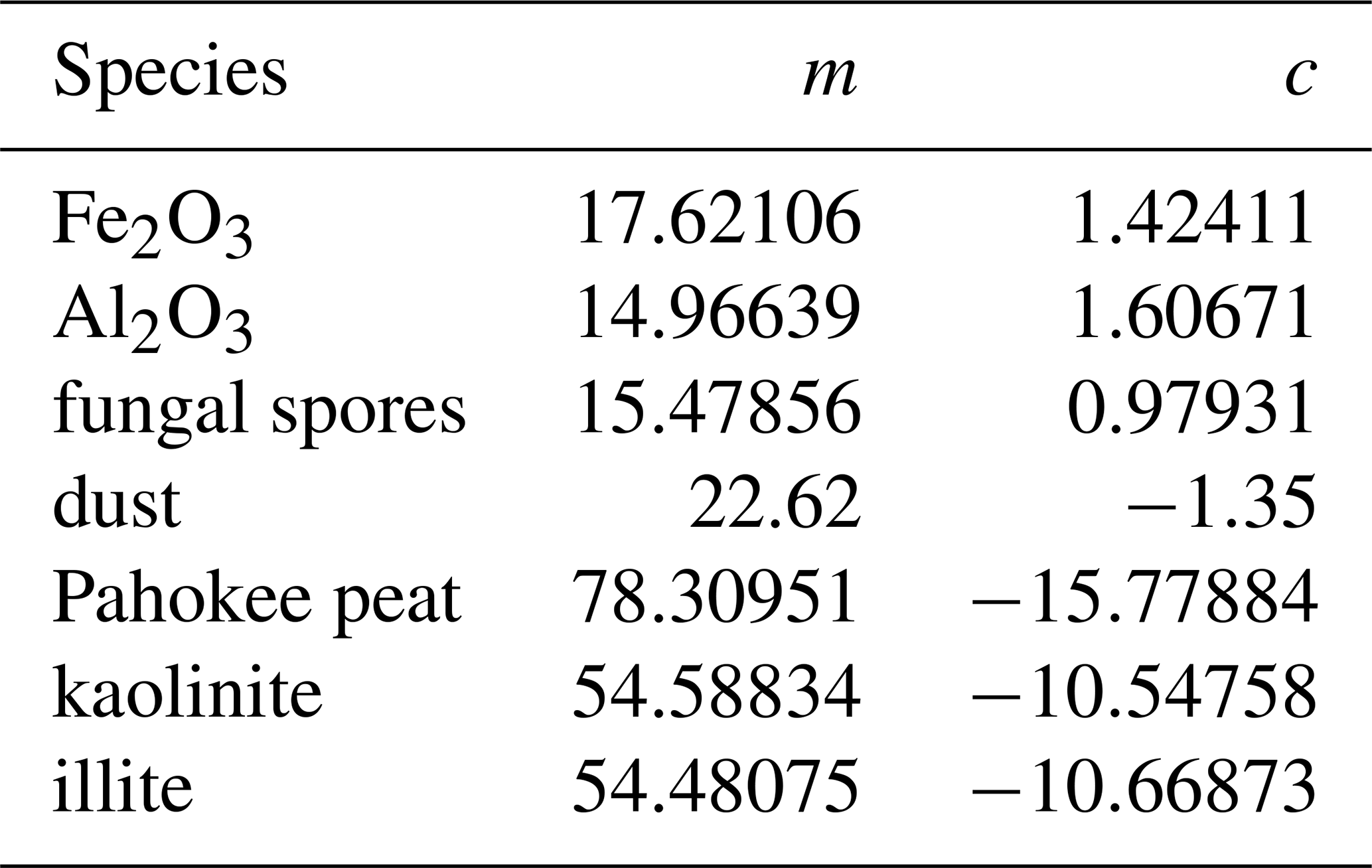
Equations (B11) and (B12), combined with Eqs. (B5) and (20), relate the metrics of immersion freezing to the INP size distribution parameters, the chemical composition of INPs, and the temperature profile, which are input parameters for PartMC. The ice crystal number concentrations and frozen fractions, as determined by Eqs. (B11) and (B12), are thus analytical solutions for scenarios where the INP population contains either a single species or multiple species in an internal mixture.

Equations (B11) and (B12) provide the framework for verifying the expected ice crystal number concentration and frozen fraction for all simulations conducted in Sect. 5.1 (shown in Table 2), except Cases 3 and 7 (because these involve two modes of INPs). The cases differ in the species combinations and temperature profiles. For instance, in Case 1, where the temperature remains constant at −20 °C and the INPs consist solely of illite, the $\overline{\mathrm{\Phi }}$ in Eqs. (B11) and (B12) is

$$\begin{array}{}\text{(B13)}& \overline{\mathrm{\Phi }}\left(t\right)={\mathrm{\Phi }}_{\text{illite}}\left(t\right)=J_{\text{het}}^{\text{illite}}(-\mathrm{20}\mathrm{°}\mathrm{C})\cdot t.\end{array}$$

In Case 6, a linear temperature decrease (2 K min⁻¹) is applied and only Fe₂O₃ is present. Therefore $\overline{\mathrm{\Phi }}$ is

$$\begin{array}{}\text{(B14)}& \overline{\mathrm{\Phi }}\left(t\right)={\mathrm{\Phi }}_{{\mathrm{Fe}}_{\mathrm{2}}{\mathrm{O}}_{\mathrm{3}}}\left(t\right)={\int }_{\mathrm{0}}^t{J}_{\text{het}}^{{\mathrm{Fe}}_{\mathrm{2}}{\mathrm{O}}_{\mathrm{3}}}\left(T\right(\mathit{\tau }\left)\right)\mathrm{d}\mathit{\tau },\end{array}$$

where, T(τ) follows the linear temperature profile. Similarly, for Case 8, which involves an internal mixture of 50 % illite and 50 % Fe₂O₃, $\overline{\mathrm{\Phi }}$ is

$$\begin{array}{}\text{(B15)}& \begin{array}{rl}\overline{\mathrm{\Phi }}\left(t\right)& ={\displaystyle \frac{\mathrm{1}}{\mathrm{2}}}({\mathrm{\Phi }}_{\text{illite}}+{\mathrm{\Phi }}_{{\mathrm{Fe}}_{\mathrm{2}}{\mathrm{O}}_{\mathrm{3}}})\\ & ={\displaystyle \frac{\mathrm{1}}{\mathrm{2}}}{\int }_{\mathrm{0}}^t{J}_{\text{het}}^{\text{illite}}\left(T\right(\mathit{\tau }\left)\right)+J_{\text{het}}^{{\mathrm{Fe}}_{\mathrm{2}}{\mathrm{O}}_{\mathrm{3}}}\left(T\right(\mathit{\tau }\left)\right)\mathrm{d}\mathit{\tau }.\end{array}\end{array}$$

The expressions for calculating the ice crystal number concentration and frozen fraction in external mixture scenarios, particularly pertaining to Cases 3 and 7, will be discussed in Appendix C in detail.

The heterogeneous ice nucleation rate coefficient used in this study is calculated with the water activity-based immersion freezing model (ABIFM) of Knopf and Alpert (2013):

$$\begin{array}{}\text{(B16)}& {\log }_{\mathrm{10}}{J}_{\text{het}}=m\cdot (a_{\mathrm{w}}-a_{\mathrm{w}}^{\text{ice}})+c,\end{array}$$

where J_het is in ${\mathrm{cm}}^{-\mathrm{2}}{\mathrm{s}}^{-\mathrm{1}}$, a_w is the water activity of the droplet, $a_{\mathrm{w}}^{\text{ice}}$ is the water activity in equilibrium with ice, and m and c are species-specific fitting parameters. Table B1 lists the values of m and c for the aerosol species used in this study.

Appendix C: Ice number concentration for multi-modal polydisperse INP population

In PartMC, a particle population can consist of multiple modes. For each mode, its size distribution, species type and mass ratio, as well as number concentration are independently specified. Assuming that the total number of modes that form a group of INPs is N_m, and the size distribution density function for the INPs in the xth mode is n_x, the size distribution density function for the entire INPs population is the sum of the density function across all modes, and the aggregate of the number concentrations from all modes equals the total number concentration of the entire INP group.

$$\begin{array}{}\text{(C1)}& {\displaystyle }{n}_{\mathrm{N}}=\sum _{x=\mathrm{1}}^{N_{\mathrm{m}}}{n}_x,\text{(C2)}& {\displaystyle }{\stackrel{\mathrm{̃}}{N}}_{\mathrm{t}}=\sum _{x=\mathrm{1}}^{N_{\mathrm{m}}}{\stackrel{\mathrm{̃}}{N}}_{\mathrm{t}}^{\left(x\right)}.\end{array}$$

By substituting Eq. (C1) into Eq. (B6), and defining ${\overline{\mathrm{\Phi }}}_x\left(t\right)$ as the weighted mean of the ice nucleation rate coefficient for the chemical components in the xth mode, we derive a general formula for the size distribution density function of activated INPs in a population with multiple modes

$$\begin{array}{}\text{(C3)}& n_{\text{frz}}(t,\ln D_{\mathrm{p}})=\sum _{x=\mathrm{1}}^{N_{\mathrm{m}}}{n}_x(t,\ln D_{\mathrm{p}})\cdot (\mathrm{1}-e^{-\mathit{\pi }{D}_{\mathrm{p}}^{\mathrm{2}}\cdot {\overline{\mathrm{\Phi }}}_x\left(t\right)}).\end{array}$$

Similarly, we can derive formulas for both the ice crystal number concentration and the frozen fraction for an INP population with multiple modes by substituting Eq. (C3) into Eqs. (B7) and (B8),

$$\begin{array}{}\text{(C4)}& {\displaystyle }\begin{array}{rl}{\stackrel{\mathrm{̃}}{N}}_{\text{frz}}& \left(t\right)=\\ & {\stackrel{\mathrm{̃}}{N}}_{\mathrm{t}}-\sum _{x=\mathrm{1}}^{N_{\mathrm{m}}}{\int }_{-\mathrm{\infty }}^{+\mathrm{\infty }}{n}_x(t,\ln D_{\mathrm{p}})\cdot e^{-\mathit{\pi }{D}_{\mathrm{p}}^{\mathrm{2}}\cdot {\overline{\mathrm{\Phi }}}_x\left(t\right)}\mathrm{d}\ln D_{\mathrm{p}};\end{array}\text{(C5)}& {\displaystyle }\begin{array}{rl}{f}_{\text{frz}}& \left(t\right)=\\ & \mathrm{1}-{\displaystyle \frac{\mathrm{1}}{{\stackrel{\mathrm{̃}}{N}}_{\mathrm{t}}}}\cdot \sum _{x=\mathrm{1}}^{N_{\mathrm{m}}}{\int }_{-\mathrm{\infty }}^{+\mathrm{\infty }}{n}_x(t,\ln D_{\mathrm{p}})\cdot e^{-\mathit{\pi }{D}_{\mathrm{p}}^{\mathrm{2}}\cdot {\overline{\mathrm{\Phi }}}_x\left(t\right)}\mathrm{d}\ln D_{\mathrm{p}}.\end{array}\end{array}$$

Assuming that the size of INPs in the xth mode follows a log-normal distribution, characterized by a number concentration ${\stackrel{\mathrm{̃}}{N}}_{\mathrm{t}}^{\left(x\right)}$, a geometric mean diameter ${\overline{D}}_{\text{pg}x}$, and a geometric standard deviation σ_gx, the size distribution density function for this mode is then given by

$$\begin{array}{}\text{(C6)}& n_x(t,\ln D_{\mathrm{p}})={\displaystyle \frac{{\stackrel{\mathrm{̃}}{N}}_{\mathrm{t}}^{\left(x\right)}}{\sqrt{\mathrm{2}\mathit{\pi }}\cdot \ln {\mathit{\sigma }}_{\mathrm{g}x}}}{e}^{-\frac{(\ln D_{\mathrm{p}}-\ln {\overline{D}}_{\text{pg}x}{)}^{\mathrm{2}}}{\mathrm{2}{\ln }^{\mathrm{2}}{\mathit{\sigma }}_{\mathrm{g}x}}}.\end{array}$$

Consequently, upon applying the assumption of a log-normal distribution for each mode, the calculations for ice crystal number concentration and frozen fraction are obtained by substituting Eq. (C6) into Eqs. (C4) and (C5), respectively.

$$\begin{array}{}\text{(C7)}& {\displaystyle }\begin{array}{rl}& {\stackrel{\mathrm{̃}}{N}}_{\text{frz}}\left(t\right)={\stackrel{\mathrm{̃}}{N}}_{\mathrm{t}}-\sum _{x=\mathrm{1}}^{N_{\mathrm{m}}}{\displaystyle \frac{{\stackrel{\mathrm{̃}}{N}}_{\mathrm{t}}^{\left(x\right)}}{\sqrt{\mathrm{2}\mathit{\pi }}\cdot \ln {\mathit{\sigma }}_{\mathrm{g}x}}}\\ & \cdot {\int }_{-\mathrm{\infty }}^{+\mathrm{\infty }}\exp \left[-{\displaystyle \frac{(\ln D_{\mathrm{p}}-\ln {\overline{D}}_{\text{pg}x}{)}^{\mathrm{2}}}{\mathrm{2}{\ln }^{\mathrm{2}}{\mathit{\sigma }}_{\mathrm{g}x}}}-\mathit{\pi }{D}_{\mathrm{p}}^{\mathrm{2}}\cdot {\overline{\mathrm{\Phi }}}_x\left(t\right)\right]\mathrm{d}\ln D_{\mathrm{p}};\end{array}\text{(C8)}& {\displaystyle }\begin{array}{rl}& f_{\text{frz}}\left(t\right)=\mathrm{1}-{\displaystyle \frac{\mathrm{1}}{{\stackrel{\mathrm{̃}}{N}}_{\mathrm{t}}}}\sum _{x=\mathrm{1}}^{N_{\mathrm{m}}}{\displaystyle \frac{{\stackrel{\mathrm{̃}}{N}}_{\mathrm{t}}^{\left(x\right)}}{\sqrt{\mathrm{2}\mathit{\pi }}\cdot \ln {\mathit{\sigma }}_{\mathrm{g}x}}}\\ & \cdot {\int }_{-\mathrm{\infty }}^{+\mathrm{\infty }}\exp \left[-{\displaystyle \frac{(\ln D_{\mathrm{p}}-\ln {\overline{D}}_{\text{pg}x}{)}^{\mathrm{2}}}{\mathrm{2}{\ln }^{\mathrm{2}}{\mathit{\sigma }}_{\mathrm{g}x}}}-\mathit{\pi }{D}_{\mathrm{p}}^{\mathrm{2}}\cdot {\overline{\mathrm{\Phi }}}_x\left(t\right)\right]\mathrm{d}\ln D_{\mathrm{p}}.\end{array}\end{array}$$

Based on the predefined parameters for the Cases 3 and 7, an externally mixed INP population in the PartMC model, composed of 50 % illite and 50 % Fe₂O₃, is created by establishing two modes. Each mode has an identical number concentration and size distribution, but differs in composition: one mode consists entirely of illite, while the other is composed solely of Fe₂O₃. Therefore, by establishing the parameters

$$\begin{array}{}\text{(C9)}& {\displaystyle }{\stackrel{\mathrm{̃}}{N}}_{\mathrm{t}}^{\left(\mathrm{1}\right)}={\stackrel{\mathrm{̃}}{N}}_{\mathrm{t}}^{\left(\mathrm{2}\right)}={\displaystyle \frac{\mathrm{1}}{\mathrm{2}}}\cdot {\stackrel{\mathrm{̃}}{N}}_{\mathrm{t}};\text{(C10)}& {\displaystyle }{\overline{D}}_{\text{pg1}}={\overline{D}}_{\text{pg2}}={\overline{D}}_{\text{pg}};\text{(C11)}& {\displaystyle }{\mathit{\sigma }}_{\text{g1}}={\mathit{\sigma }}_{\text{g2}}={\mathit{\sigma }}_{\mathrm{g}}.\end{array}$$

and substituting Eqs. (C9)–(C11) into Eqs. (C7) and (C8), we derive formulas representing the ice crystal number concentration and frozen fraction for the Case 3 and 7 as

$$\begin{array}{}\text{(C12)}& {\displaystyle }\begin{array}{rl}& {\stackrel{\mathrm{̃}}{N}}_{\text{frz}}\left(t\right)={\stackrel{\mathrm{̃}}{N}}_{\mathrm{t}}-{\displaystyle \frac{\mathrm{1}}{\mathrm{2}}}\mathit{\{}{\displaystyle \frac{{\stackrel{\mathrm{̃}}{N}}_{\mathrm{t}}}{\sqrt{\mathrm{2}\mathit{\pi }}\cdot \ln {\mathit{\sigma }}_{\mathrm{g}}}}\\ & \cdot {\int }_{-\mathrm{\infty }}^{+\mathrm{\infty }}\exp \left[-{\displaystyle \frac{(\ln D_{\mathrm{p}}-\ln {\overline{D}}_{\text{pg}}{)}^{\mathrm{2}}}{\mathrm{2}(\ln {\mathit{\sigma }}_{\mathrm{g}}{)}^{\mathrm{2}}}}-\mathit{\pi }{D}_{\mathrm{p}}^{\mathrm{2}}\cdot {\mathrm{\Phi }}_{\text{illite}}\left(T\right(t\left)\right)\right]\mathrm{d}\ln D_{\mathrm{p}}\\ & +{\displaystyle \frac{{\stackrel{\mathrm{̃}}{N}}_{\mathrm{t}}}{\sqrt{\mathrm{2}\mathit{\pi }}\cdot \ln {\mathit{\sigma }}_{\mathrm{g}}}}\\ & \cdot {\int }_{-\mathrm{\infty }}^{+\mathrm{\infty }}\exp \left[-{\displaystyle \frac{(\ln D_{\mathrm{p}}-\ln {\overline{D}}_{\text{pg}}{)}^{\mathrm{2}}}{\mathrm{2}(\ln {\mathit{\sigma }}_{\mathrm{g}}{)}^{\mathrm{2}}}}-\mathit{\pi }{D}_{\mathrm{p}}^{\mathrm{2}}\cdot {\mathrm{\Phi }}_{{\mathrm{Fe}}_{\mathrm{2}}{\mathrm{O}}_{\mathrm{3}}}\left(T\right(t\left)\right)\right]\mathrm{d}\ln D_{\mathrm{p}}\mathit{\}};\end{array}\text{(C13)}& {\displaystyle }\begin{array}{rl}& f_{\text{frz}}\left(t\right)=\mathrm{1}-{\displaystyle \frac{\mathrm{1}}{\mathrm{2}}}\mathit{\{}{\displaystyle \frac{\mathrm{1}}{\sqrt{\mathrm{2}\mathit{\pi }}\cdot \ln {\mathit{\sigma }}_{\mathrm{g}}}}\\ & \cdot {\int }_{-\mathrm{\infty }}^{+\mathrm{\infty }}\exp \left[-{\displaystyle \frac{(\ln D_{\mathrm{p}}-\ln {\overline{D}}_{\text{pg}}{)}^{\mathrm{2}}}{\mathrm{2}(\ln {\mathit{\sigma }}_{\mathrm{g}}{)}^{\mathrm{2}}}}-\mathit{\pi }{D}_{\mathrm{p}}^{\mathrm{2}}\cdot {\mathrm{\Phi }}_{\text{illite}}\left(T\right(t\left)\right)\right]\mathrm{d}\ln D_{\mathrm{p}}\\ & +{\displaystyle \frac{\mathrm{1}}{\sqrt{\mathrm{2}\mathit{\pi }}\cdot \ln {\mathit{\sigma }}_{\mathrm{g}}}}\\ & \cdot {\int }_{-\mathrm{\infty }}^{+\mathrm{\infty }}\exp \left[-{\displaystyle \frac{(\ln D_{\mathrm{p}}-\ln {\overline{D}}_{\text{pg}}{)}^{\mathrm{2}}}{\mathrm{2}(\ln {\mathit{\sigma }}_{\mathrm{g}}{)}^{\mathrm{2}}}}-\mathit{\pi }{D}_{\mathrm{p}}^{\mathrm{2}}\cdot {\mathrm{\Phi }}_{{\mathrm{Fe}}_{\mathrm{2}}{\mathrm{O}}_{\mathrm{3}}}\left(T\right(t\left)\right)\right]\mathrm{d}\ln D_{\mathrm{p}}\mathit{\}}.\end{array}\end{array}$$

The terms Φ_illite(T(t)) and ${\mathrm{\Phi }}_{{\mathrm{Fe}}_{\mathrm{2}}{\mathrm{O}}_{\mathrm{3}}}\left(T\right(t\left)\right)$ refer to the time integration of the ice nucleation rate coefficient of illite and Fe₂O₃, respectively.

Equations (C12) and (C13) provide the general formulas applicable to Cases 3 and 7, which differ in their respective temperature profiles, T(t).

Appendix D: Proof of Theorem 1

The symbols used in this proof are listed in the Table D1.

Based on the definitions in Table D1, there are:

$$\begin{array}{}\text{(D1)}& {\displaystyle }\sum _{i=\mathrm{1}}^{N_{\mathrm{s}}}{w}_j^{\left(i\right)}=\mathrm{1},\text{ for }\forall j\in [\mathrm{1},N_{\mathrm{p}}]\text{(D2)}& {\displaystyle }\sum _{j=\mathrm{1}}^{N_{\mathrm{p}}}{S}_{{\mathrm{p}}_j}{w}_j^{\left(i\right)}=\sum _{j=\mathrm{1}}^{N_{\mathrm{p}}}\mathit{\pi }{D}_{\mathrm{p}}^{\mathrm{2}}{w}_j^{\left(i\right)}=S^{\left(i\right)},\text{ for }\forall i\in [\mathrm{1},N_{\mathrm{s}}]\text{(D3)}& {\displaystyle }\mathrm{0}\le w_j^{\left(i\right)}\le \mathrm{1},\text{ for }\forall i\in [\mathrm{1},N_{\mathrm{s}}],\forall j\in [\mathrm{1},N_{\mathrm{p}}].\end{array}$$

A series of $w_j^{\left(i\right)}$ must satisfy Eqs. (D1), (D2), and (D3) to represent a meaningful mixing state.

Table D1 Particle surface and surface fraction definitions and notations.

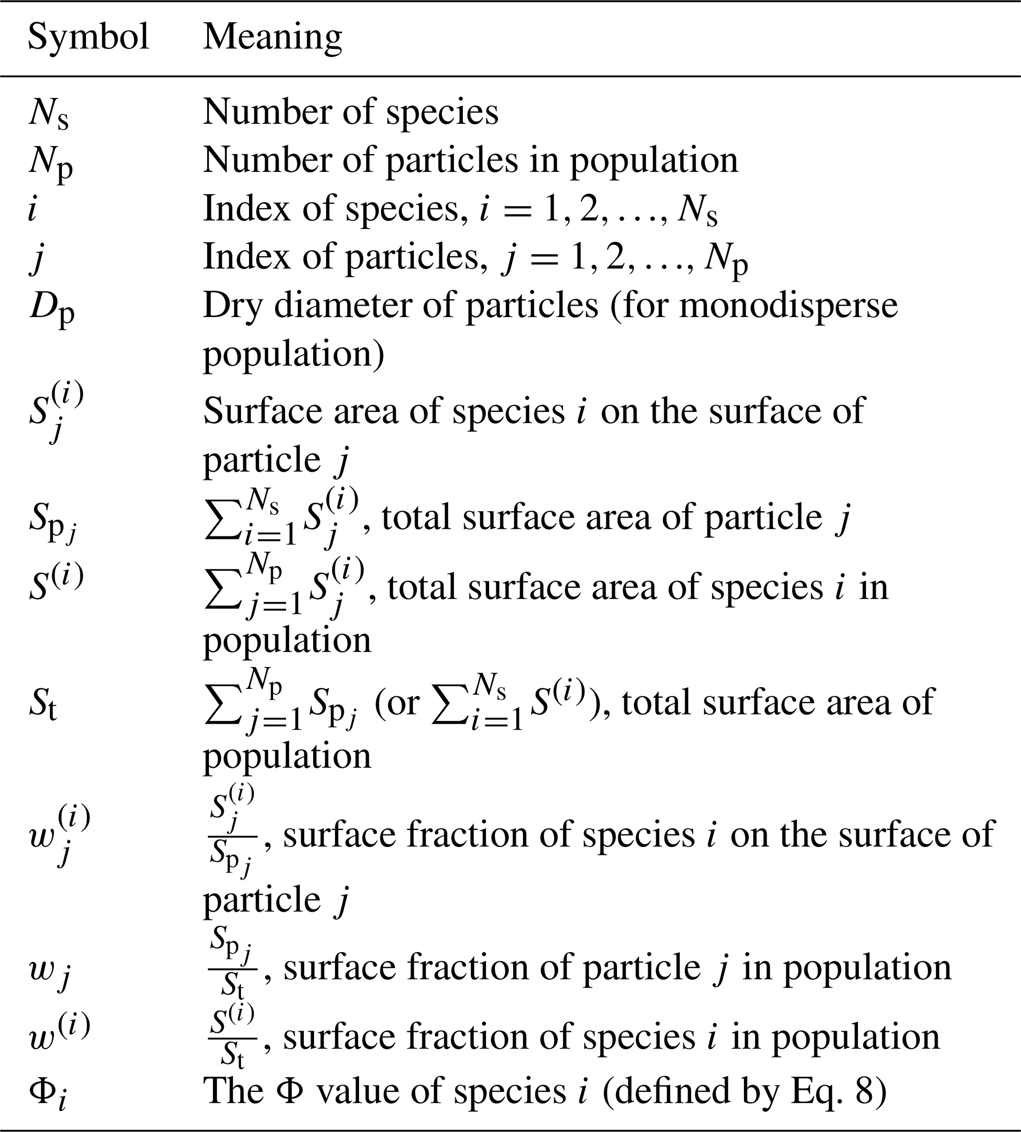
Here are the assumptions in this proof: First: S⁽ⁱ⁾, $i=\mathrm{1},\mathrm{2},\mathrm{\dots },N_{\mathrm{s}}$ are constants, and satisfying ${\sum }_{i=\mathrm{1}}^{N_{\mathrm{s}}}{S}^{\left(i\right)}=\mathit{\pi }{D}_{\mathrm{p}}^{\mathrm{2}}{N}_{\mathrm{p}}$ to make sure the sum of each species' total surface equals the sum of particle's surface. Second: For each species i ($i=\mathrm{1},\mathrm{2},\mathrm{\dots },N_{\mathrm{s}}$), $\frac{S^{\left(i\right)}}{\mathit{\pi }{D}_{\mathrm{p}}^{\mathrm{2}}}$ is an integer to make sure each species covers an integer number of particles in the external mixture. Third: Assume ${\mathrm{\Phi }}_{\mathrm{1}}\ne {\mathrm{\Phi }}_{\mathrm{2}}\ne \mathrm{\dots }\ne {\mathrm{\Phi }}_{N_{\mathrm{s}}}$ to avoid some mathematical complexity, if two species do have the same Φ value, just regard them as the same species, which would not affect our result.

We divide the proof of Theorem 1 into two parts – Theorem 1A and Theorem 1B – which demonstrate that the internal mixture is the most efficient mixing state and the external mixture is the least efficient, respectively.

Theorem 1A.  For monodisperse INP populations, the internal mixture is the most efficient mixing state.

.

The topic of the most efficient mixing state in terms of frozen fraction can be converted to an optimization problem:

Optimization 1

$$\begin{array}{}\text{(D4)}& \underset{w_j^{\left(i\right)}\in [\mathrm{0},\mathrm{1}]}{max}\mathrm{1}-{\displaystyle \frac{\mathrm{1}}{N_{\mathrm{p}}}}\sum _{j=\mathrm{1}}^{N_{\mathrm{p}}}\exp \left(-\mathit{\pi }{D}_{\mathrm{p}}^{\mathrm{2}}\sum _{i=\mathrm{1}}^{N_{\mathrm{s}}}{w}_j^{\left(i\right)}{\mathrm{\Phi }}_i\right)\end{array}$$

$$\begin{array}{}\text{(D5)}& {\displaystyle }s.t.& {\displaystyle }\sum _{i=\mathrm{1}}^{N_{\mathrm{s}}}{w}_j^{\left(i\right)}=\mathrm{1}\text{(D6)}& {\displaystyle }& {\displaystyle }\sum _{j=\mathrm{1}}^{N_{\mathrm{p}}}{w}_j^{\left(i\right)}={\displaystyle \frac{S^{\left(i\right)}}{\mathit{\pi }{D}_{\mathrm{p}}^{\mathrm{2}}}}\end{array}$$

Define $f_{\text{frz}}^{\text{(max)}}$ as the maximum solution of Optimization 1. Since $\exp (-\mathit{\pi }{D}_{\mathrm{p}}^{\mathrm{2}}\cdot {\sum }_{i=\mathrm{1}}^{N_{\mathrm{s}}}{w}_j^{\left(i\right)}{\mathrm{\Phi }}_i)=P_{\text{unf},j}$, combining with Eq. (D2), there is:

$$\begin{array}{ll}{\displaystyle }\prod _{j=\mathrm{1}}^{N_{\mathrm{p}}}{P}_{\text{unf},j}& {\displaystyle }=\prod _{j=\mathrm{1}}^{N_{\mathrm{p}}}\exp \left(-\mathit{\pi }{D}_{\mathrm{p}}^{\mathrm{2}}\sum _{i=\mathrm{1}}^{N_{\mathrm{s}}}{w}_j^{\left(i\right)}{\mathrm{\Phi }}_i\right)\\ \text{(D7)}& {\displaystyle }& {\displaystyle }=\exp \left(-\mathit{\pi }{D}_{\mathrm{p}}^{\mathrm{2}}\sum _{j=\mathrm{1}}^{N_{\mathrm{p}}}\sum _{i=\mathrm{1}}^{N_{\mathrm{s}}}{w}_j^{\left(i\right)}{\mathrm{\Phi }}_i\right){\displaystyle }& {\displaystyle }=\exp \left[-\sum _{i=\mathrm{1}}^{N_{\mathrm{s}}}{\mathrm{\Phi }}_i\cdot \left(\mathit{\pi }{D}_{\mathrm{p}}^{\mathrm{2}}\cdot \sum _{j=\mathrm{1}}^{N_{\mathrm{p}}}{w}_j^{\left(i\right)}\right)\right]\\ \text{(D8)}& {\displaystyle }& {\displaystyle }=\exp \left(-\sum _{i=\mathrm{1}}^{N_{\mathrm{s}}}{S}^{\left(i\right)}{\mathrm{\Phi }}_i\right)=\text{constant}.\end{array}$$

It is a constant because it depends only on the total surface area of each species S⁽ⁱ⁾, which is fixed in Optimization 1 and independent of how this surface area is distributed among particles (i.e., independent of the mixing state). We therefore define this constant as 𝒦:

$$\begin{array}{}\text{(D9)}& \mathcal{K}=\exp \left(-\sum _{i=\mathrm{1}}^{N_{\mathrm{s}}}{S}^{\left(i\right)}{\mathrm{\Phi }}_i\right),\end{array}$$

we can propose another optimization problem:

Optimization 2

$$\begin{array}{}\text{(D10)}& {\displaystyle }\underset{P_{\text{unf,}j}\in [\mathrm{0},\mathrm{1}]}{max}\mathrm{1}-{\displaystyle \frac{\mathrm{1}}{N_{\mathrm{p}}}}\sum _{j=\mathrm{1}}^{N_{\mathrm{p}}}{P}_{\text{unf},j}\text{(D11)}& {\displaystyle }s.t.\prod _{j=\mathrm{1}}^{N_{\mathrm{p}}}{P}_{\text{unf},j}=\mathcal{K}\end{array}$$

and define $f_{\text{frz}}^{*}$ is the solution of this problem. It is worth noting that since there are

$$\begin{array}{}\text{(D12)}& {\displaystyle }\begin{array}{rl}\mathrm{1}-{\displaystyle \frac{\mathrm{1}}{N_{\mathrm{p}}}}\sum _{j=\mathrm{1}}^{N_{\mathrm{p}}}& \exp \left(-\mathit{\pi }{D}_{\mathrm{p}}^{\mathrm{2}}\sum _{i=\mathrm{1}}^{N_{\mathrm{s}}}{w}_j^{\left(i\right)}{\mathrm{\Phi }}_i\right)\\ & \equiv \mathrm{1}-{\displaystyle \frac{\mathrm{1}}{N_{\mathrm{p}}}}\sum _{j=\mathrm{1}}^{N_{\mathrm{p}}}{P}_{\text{unf},j},\end{array}\text{(D13)}& {\displaystyle }\sum _{j=\mathrm{1}}^{N_{\mathrm{p}}}{w}_j^{\left(i\right)}={\displaystyle \frac{S^{\left(i\right)}}{\mathit{\pi }{D}_{\mathrm{p}}^{\mathrm{2}}}}\iff \prod _{j=\mathrm{1}}^{N_{\mathrm{p}}}{P}_{\text{unf},j}=\mathcal{K},\end{array}$$

the Optimization 2 only lost the constraint of Eq. (D5), therefore, there is

$$\begin{array}{}\text{(D14)}& f_{\text{frz}}^{*}\ge f_{\text{frz}}^{\text{(max)}}.\end{array}$$

Now, we solve Optimization 2. Based on the AM–GM relationship, there is

$$\begin{array}{}\text{(D15)}& {\displaystyle \frac{\mathrm{1}}{N_{\mathrm{p}}}}\sum _{j=\mathrm{1}}^{N_{\mathrm{p}}}{P}_{\text{unf},j}\ge {\left(\prod _{j=\mathrm{1}}^{N_{\mathrm{p}}}{P}_{\text{unf},j}\right)}^{\frac{\mathrm{1}}{N_{\mathrm{p}}}}={\mathcal{K}}^{\frac{\mathrm{1}}{N_{\mathrm{p}}}},\end{array}$$

with equality if and only if

$$\begin{array}{}\text{(D16)}& P_{\text{unf,}\mathrm{1}}=P_{\text{unf,}\mathrm{2}}=\mathrm{\dots }=P_{\text{unf,}{N}_{\mathrm{p}}}={\mathcal{K}}^{\frac{\mathrm{1}}{N_{\mathrm{p}}}}.\end{array}$$

Therefore, $\mathrm{1}-\frac{\mathrm{1}}{N_{\mathrm{p}}}{\sum }_{j=\mathrm{1}}^{N_{\mathrm{p}}}{P}_{\text{unf},j}$ attains its maximum only when Eq. (D16) holds. Thus, we have

$$\begin{array}{}\text{(D17)}& \begin{array}{rl}{P}_{\text{unf},j}^{*}& ={\mathcal{K}}^{\frac{\mathrm{1}}{N_{\mathrm{p}}}}\\ & =\exp \left(-{\displaystyle \frac{\mathrm{1}}{N_{\mathrm{p}}}}\sum _{i=\mathrm{1}}^{N_{\mathrm{s}}}{S}^{\left(i\right)}{\mathrm{\Phi }}_i\right),\text{ for }\forall j\in [\mathrm{1},N_{\mathrm{p}}].\end{array}\end{array}$$

Therefore, when each particle has the same unfrozen (or freezing) probability, Eq. (D10) in Optimization 2 reaches its maximum, where

$$\begin{array}{}\text{(D18)}& \begin{array}{rl}{f}_{\text{frz}}^{*}& =\mathrm{1}-{\displaystyle \frac{\mathrm{1}}{N_{\mathrm{p}}}}\sum _{j=\mathrm{1}}^{N_{\mathrm{p}}}{P}_{\text{unf},j}^{*}=\mathrm{1}-{\mathcal{K}}^{\frac{\mathrm{1}}{N_{\mathrm{p}}}}\\ & =\mathrm{1}-\exp \left(-{\displaystyle \frac{\mathrm{1}}{N_{\mathrm{p}}}}\sum _{i=\mathrm{1}}^{N_{\mathrm{s}}}{S}^{\left(i\right)}{\mathrm{\Phi }}_i\right).\end{array}\end{array}$$

For the internal mixture, which, defined in Riemer and West (2013), satisfies

$$\begin{array}{}\text{(D19)}& w_j^{\left(i\right)}={\displaystyle \frac{S^{\left(i\right)}}{\mathit{\pi }{D}_{\mathrm{p}}^{\mathrm{2}}{N}_{\mathrm{p}}}}\text{ for }\forall j\in [\mathrm{1},N_{\mathrm{p}}],\forall i\in [\mathrm{1},N_{\mathrm{s}}].\end{array}$$

Define the frozen fraction of internal mixture as $f_{\text{frz}}^{\text{(int)}}$, there is

$$\begin{array}{}\text{(D20)}& \begin{array}{rl}{f}_{\text{frz}}^{\text{(int)}}& =\mathrm{1}-{\displaystyle \frac{\mathrm{1}}{N_{\mathrm{p}}}}\sum _{j=\mathrm{1}}^{N_{\mathrm{p}}}\exp \left(-\mathit{\pi }{D}_{\mathrm{p}}^{\mathrm{2}}\cdot \sum _{i=\mathrm{1}}^{N_{\mathrm{s}}}{w}_j^{\left(i\right)}{\mathrm{\Phi }}_i\right)\\ & =\mathrm{1}-{\displaystyle \frac{\mathrm{1}}{N_{\mathrm{p}}}}\sum _{j=\mathrm{1}}^{N_{\mathrm{p}}}\exp \left(-\mathit{\pi }{D}_{\mathrm{p}}^{\mathrm{2}}\cdot \sum _{i=\mathrm{1}}^{N_{\mathrm{s}}}{\displaystyle \frac{S^{\left(i\right)}}{\mathit{\pi }{D}_{\mathrm{p}}^{\mathrm{2}}{N}_{\mathrm{p}}}}\cdot {\mathrm{\Phi }}_i\right)\\ & =\mathrm{1}-\exp \left(-{\displaystyle \frac{\mathrm{1}}{N_{\mathrm{p}}}}\sum _{i=\mathrm{1}}^{N_{\mathrm{s}}}{S}^{\left(i\right)}{\mathrm{\Phi }}_i\right),\end{array}\end{array}$$

therefore, $f_{\text{frz}}^{\text{(int)}}=f_{\text{frz}}^{*}$. In addition, since the internal mixture shown in Eq. (D19) satisfies the constraints in Optimization 1 (Eqs. D5 and D6), i.e., it is a valid mixing state, there must be

$$\begin{array}{}\text{(D21)}& f_{\text{frz}}^{\text{(int)}}=f_{\text{frz}}^{*}\le f_{\text{frz}}^{\text{(max)}},\end{array}$$

combining Eq. (D14), we have:

$$\begin{array}{}\text{(D22)}& f_{\text{frz}}^{\text{(int)}}=f_{\text{frz}}^{*}=f_{\text{frz}}^{\text{(max)}}.\end{array}$$

Therefore, the internal mixture is the most efficient mixing state for monodisperse particle population.

Theorem 1B.  For monodisperse INP populations, the external mixture is the least efficient mixing state.

.

According to the definition of external mixture in Riemer and West (2013), there is

$$\begin{array}{rl}\text{External mixture}\iff w_j^{\left(i\right)}& =\mathrm{0}\text{ or }\mathrm{1},\sum _{i=\mathrm{1}}^{N_{\mathrm{s}}}{w}_j^{\left(i\right)}=\mathrm{1},\\ & \text{ for }\forall i\in [\mathrm{1},N_{\mathrm{s}}],\forall j\in [\mathrm{1},N_{\mathrm{p}}].\end{array}$$

Define the frozen fraction of external mixture is denoted as $f_{\text{frz}}^{\text{(ext)}}$, based on Eq. (12), we have

$$\begin{array}{}\text{(D23)}& \begin{array}{rl}{f}_{\text{frz}}^{\text{(ext)}}& =\mathrm{1}-\sum _{i=\mathrm{1}}^{N_{\mathrm{s}}}{w}^{\left(i\right)}{P}_{\text{unf},j}\\ & =\mathrm{1}-\sum _{i=\mathrm{1}}^{N_{\mathrm{s}}}{\displaystyle \frac{S^{\left(i\right)}}{\mathit{\pi }{D}_{\mathrm{p}}^{\mathrm{2}}{N}_{\mathrm{p}}}}\cdot \exp (-\mathit{\pi }{D}_{\mathrm{p}}^{\mathrm{2}}{\mathrm{\Phi }}_i).\end{array}\end{array}$$

We prove the Theorem 1B by contradiction. Assuming a mixing state of monodisperse particle population, described by ${\stackrel{\mathrm{̃}}{w}}_j^{\left(i\right)}$, $i=\mathrm{1},\mathrm{2},\mathrm{\dots },N_{\mathrm{s}}$, $j=\mathrm{1},\mathrm{2},\mathrm{\dots },N_{\mathrm{p}}$, is the least efficient mixing state but is not the external mixture. Define the frozen fraction

$$\begin{array}{}\text{(D24)}& {\stackrel{\mathrm{̃}}{f}}_{\text{frz}}=\mathrm{1}-{\displaystyle \frac{\mathrm{1}}{N_{\mathrm{p}}}}\sum _{j=\mathrm{1}}^{N_{\mathrm{p}}}\exp \left(-\mathit{\pi }{D}_{\mathrm{p}}^{\mathrm{2}}\sum _{i=\mathrm{1}}^{N_{\mathrm{s}}}{\stackrel{\mathrm{̃}}{w}}_j^{\left(i\right)}{\mathrm{\Phi }}_i\right).\end{array}$$

Since it is different with external mixture, there must be

$$\exists i\in [\mathrm{1},N_{\mathrm{s}}],\exists j\in [\mathrm{1},N_{\mathrm{p}}],\mathrm{0}<{\stackrel{\mathrm{̃}}{w}}_j^{\left(i\right)}<\mathrm{1},$$

in other words, at least one particle must contain more than one species, such that the surface area ratio of each species within that particle is less than 1. We refer to it as “mixed particle” thereafter. Define the set ${\stackrel{\mathrm{̃}}{M}}_{ix}=\mathit{\left\{}i\right|\exists j\in [\mathrm{1},N_{\mathrm{p}}],\mathrm{0}<{\stackrel{\mathrm{̃}}{w}}_j^{\left(i\right)}<\mathrm{1}\mathit{\}}$ representing the set of species indices among all mixed particles, there must be ${\stackrel{\mathrm{̃}}{M}}_{ix}\ne \mathrm{\varnothing }$. Define $i_{\mathrm{0}}=\arg \underset{i\in {\stackrel{\mathrm{̃}}{M}}_{ix}}{min}{\mathrm{\Phi }}_i$, there is $\exists j_{\mathrm{A}}\in [\mathrm{1},N_{\mathrm{p}}],\mathrm{0}<{\stackrel{\mathrm{̃}}{w}}_{j_{\mathrm{A}}}^{\left(i_{\mathrm{0}}\right)}<\mathrm{1}$, by the definition of ${\stackrel{\mathrm{̃}}{M}}_{ix}$. According to the assumption of $\frac{S_{i_{\mathrm{0}}}}{\mathit{\pi }{D}_{\mathrm{p}}^{\mathrm{2}}}$ is an integer, there must be $\exists j_{\mathrm{B}}\in [\mathrm{1},N_{\mathrm{p}}]$, j_B≠j_A, and $\mathrm{0}<{\stackrel{\mathrm{̃}}{w}}_{j_{\mathrm{B}}}^{\left(i_{\mathrm{0}}\right)}<\mathrm{1}$, otherwise, ${\sum }_{j=\mathrm{1},j\ne j_{\mathrm{A}}}^{N_{\mathrm{p}}}{\stackrel{\mathrm{̃}}{w}}_j^{\left(i_{\mathrm{0}}\right)}$ must be an integer and $\frac{S_{i_{\mathrm{0}}}}{\mathit{\pi }{D}_{\mathrm{p}}^{\mathrm{2}}}=\frac{{\sum }_{j=\mathrm{1}}^{N_{\mathrm{p}}}{\stackrel{\mathrm{̃}}{w}}_j^{\left(i_{\mathrm{0}}\right)}\cdot \mathit{\pi }{D}_{\mathrm{p}}^{\mathrm{2}}}{\mathit{\pi }{D}_{\mathrm{p}}^{\mathrm{2}}}={\sum }_{j=\mathrm{1}}^{N_{\mathrm{p}}}{\stackrel{\mathrm{̃}}{w}}_j^{\left(i_{\mathrm{0}}\right)}={\stackrel{\mathrm{̃}}{w}}_{j_{\mathrm{A}}}^{\left(i_{\mathrm{0}}\right)}+{\sum }_{j=\mathrm{1},j\ne j_{\mathrm{A}}}^{N_{\mathrm{p}}}{\stackrel{\mathrm{̃}}{w}}_j^{\left(i_{\mathrm{0}}\right)}$ would not be an integer. In other words, there must be at least two mixed particles. If there were only one mixed particle, one of our assumptions would be violated – we could not form a strict external mixture. Since there are at least two such particles, we can select two of them that both contain species i₀, and denote their indices by j_A and j_B, respectively (The above argument shows that such particles j_A and j_B must exist).

We assume $P_{\text{unf,}{j}_{\mathrm{A}}}\ge P_{\text{unf,}{j}_{\mathrm{B}}}$ (i.e., $P_{\text{frz,}{j}_{\mathrm{A}}}\le P_{\text{frz,}{j}_{\mathrm{B}}}$), if not, we can just switch the index of j_A and j_B for these two particles. Now, we look at the particle j_A and j_B, define $A_{j_{\mathrm{A}}}=\mathit{\left\{}i\right|{\stackrel{\mathrm{̃}}{w}}_{j_{\mathrm{A}}}^{\left(i\right)}>\mathrm{0},i\in [\mathrm{1},N_{\mathrm{s}}]\mathit{\}}$, $A_{j_{\mathrm{B}}}=\mathit{\left\{}i\right|{\stackrel{\mathrm{̃}}{w}}_{j_{\mathrm{B}}}^{\left(i\right)}>\mathrm{0},i\in [\mathrm{1},N_{\mathrm{s}}]\mathit{\}}$, are the set of species index that particle A and B contains, respectively. Since $\mathrm{0}<{\stackrel{\mathrm{̃}}{w}}_{j_{\mathrm{A}}}^{\left(i_{\mathrm{0}}\right)}<\mathrm{1}$ and ${\sum }_{i=\mathrm{1}}^{N_{\mathrm{s}}}{\stackrel{\mathrm{̃}}{w}}_{j_{\mathrm{A}}}^{\left(i\right)}=\mathrm{1}$, for $\forall i_{\mathrm{A}}\in A_{j_{\mathrm{A}}}$, there is $\mathrm{0}<{\stackrel{\mathrm{̃}}{w}}_{j_{\mathrm{A}}}^{\left(i_{\mathrm{A}}\right)}<\mathrm{1}$, therefore, for $\forall i_{\mathrm{A}}\in A_{j_{\mathrm{A}}}$, $i_{\mathrm{A}}\in {\stackrel{\mathrm{̃}}{M}}_{ix}$, and there is ${\mathrm{\Phi }}_{i_{\mathrm{0}}}<{\mathrm{\Phi }}_{i_{\mathrm{A}}}$ according to the definition of i₀. Similarly, there also be $\forall i_{\mathrm{B}}\in A_{j_{\mathrm{B}}}$, $i_{\mathrm{B}}\in {\stackrel{\mathrm{̃}}{M}}_{ix}$, and ${\mathrm{\Phi }}_{i_{\mathrm{0}}}<{\mathrm{\Phi }}_{i_{\mathrm{B}}}$. This implies that, when we define

$$\begin{array}{}\text{(D25)}& {\overline{\mathrm{\Phi }}}_{j_{\mathrm{A}}}^{(i\ne i_{\mathrm{0}})}={\displaystyle \frac{\mathrm{1}}{{\sum }_{i=\mathrm{1},i\ne i_{\mathrm{0}}}^{N_{\mathrm{s}}}{\stackrel{\mathrm{̃}}{w}}_{j_{\mathrm{A}}}^{\left(i\right)}}}\sum _{i=\mathrm{1},i\ne i_{\mathrm{0}}}^{N_{\mathrm{s}}}{\stackrel{\mathrm{̃}}{w}}_{j_{\mathrm{A}}}^{\left(i\right)}{\mathrm{\Phi }}_i,\end{array}$$

there must be ${\mathrm{\Phi }}_{i_{\mathrm{0}}}<{\overline{\mathrm{\Phi }}}_{j_{\mathrm{A}}}^{(i\ne i_{\mathrm{0}})}$. This statement holds because i₀ is defined as the species with the smallest Φ among all species present in mixed particles. Since the other species contained in particle j_A also belong to this set, the average Φ of those species, ${\overline{\mathrm{\Phi }}}_{j_{\mathrm{A}}}^{(i\ne i_{\mathrm{0}})}$ must be greater than ${\mathrm{\Phi }}_{i_{\mathrm{0}}}$.

Now, we construct a new mixing state, described as ${\widehat{w}}_j^{\left(i\right)}$, $i=\mathrm{1},\mathrm{2},\mathrm{\dots },N_{\mathrm{s}}$, $j=\mathrm{1},\mathrm{2},\mathrm{..},N_{\mathrm{p}}$, such that

$$\begin{array}{}\text{(D26)}& {\widehat{w}}_j^{\left(i\right)}=\left\{\begin{array}{ll}{\stackrel{\mathrm{̃}}{w}}_{j_{\mathrm{A}}}^{\left(i_{\mathrm{0}}\right)}+\mathit{\delta }w,& j=j_{\mathrm{A}},i=i_{\mathrm{0}};\\ {\stackrel{\mathrm{̃}}{w}}_{j_{\mathrm{A}}}^{\left(i\right)}-\mathit{\delta }w\cdot \frac{{\stackrel{\mathrm{̃}}{w}}_{j_{\mathrm{A}}}^{\left(i\right)}}{{\sum }_{i^{\prime }=\mathrm{1},i^{\prime }\ne i_{\mathrm{0}}}^{N_{\mathrm{s}}}{\stackrel{\mathrm{̃}}{w}}_{j_{\mathrm{A}}}^{\left(i\right)}},& j=j_{\mathrm{A}},i\ne i_{\mathrm{0}};\\ {\stackrel{\mathrm{̃}}{w}}_{j_{\mathrm{B}}}^{\left(i_{\mathrm{0}}\right)}-\mathit{\delta }w,& j=j_{\mathrm{B}},i=i_{\mathrm{0}};\\ {\stackrel{\mathrm{̃}}{w}}_{j_{\mathrm{B}}}^{\left(i\right)}+\mathit{\delta }w\cdot \frac{{\stackrel{\mathrm{̃}}{w}}_{j_{\mathrm{A}}}^{\left(i\right)}}{{\sum }_{i^{\prime }=\mathrm{1},i^{\prime }\ne i_{\mathrm{0}}}^{N_{\mathrm{s}}}{\stackrel{\mathrm{̃}}{w}}_{j_{\mathrm{A}}}^{\left(i\right)}},& j=j_{\mathrm{B}},i\ne i_{\mathrm{0}};\\ {\stackrel{\mathrm{̃}}{w}}_j^{\left(i\right)},& j\ne j_{\mathrm{A}},j\ne j_{\mathrm{B}},\end{array}\right.\end{array}$$

where $\mathit{\delta }w=min\mathit{\{}{\stackrel{\mathrm{̃}}{w}}_{j_{\mathrm{A}}}^{\left(i_{\mathrm{0}}\right)},\mathrm{1}-{\stackrel{\mathrm{̃}}{w}}_{j_{\mathrm{A}}}^{\left(i_{\mathrm{0}}\right)},{\stackrel{\mathrm{̃}}{w}}_{j_{\mathrm{B}}}^{\left(i_{\mathrm{0}}\right)},\mathrm{1}-{\stackrel{\mathrm{̃}}{w}}_{j_{\mathrm{B}}}^{\left(i_{\mathrm{0}}\right)}\mathit{\}}$ (satisfies $\mathrm{0}<\mathit{\delta }w<\mathrm{1}$). Since ${\sum }_{i=\mathrm{1}}^{N_{\mathrm{s}}}{\widehat{w}}_j^{\left(i\right)}={\sum }_{i=\mathrm{1}}^{N_{\mathrm{s}}}{\stackrel{\mathrm{̃}}{w}}_j^{\left(i\right)}=\mathrm{1}$ for $\forall j\in [\mathrm{1},N_{\mathrm{p}}]$, ${\sum }_{j=\mathrm{1}}^{N_{\mathrm{p}}}{\widehat{w}}_j^{\left(i\right)}={\sum }_{j=\mathrm{1}}^{N_{\mathrm{p}}}{\stackrel{\mathrm{̃}}{w}}_j^{\left(i\right)}=\frac{S^{\left(i\right)}}{\mathit{\pi }{D}_{\mathrm{p}}^{\mathrm{2}}}$ for $\forall i\in [\mathrm{1},N_{\mathrm{s}}]$, and $\mathrm{0}\le {\stackrel{\mathrm{̃}}{w}}_j^{\left(i\right)}\le \mathrm{1}$ for $\forall i\in [\mathrm{1},N_{\mathrm{s}}]$, $\forall j\in [\mathrm{1},N_{\mathrm{p}}]$, Eq. (D26) represents a meaningful mixing state satisfying Eqs. (D1), (D2), and (D3). This new mixing state can be understood as a surface-area exchange between particles j_A and j_B relative to the original mixing state. In essence, making one particle less efficient and the other more efficient increases the sum of their probabilities of remaining unfrozen. As a result, the new configuration has a higher unfrozen fraction (and thus a lower frozen fraction) than the original one. The external mixture therefore represents the least efficient mixing state. Specifically, a surface area corresponding to a fraction δw of the particle surface area is exchanged between the two particles. We transfer an area $\mathit{\pi }{D}_{\mathrm{p}}^{\mathrm{2}}\mathit{\delta }w$ of species i₀ from particle j_B to particle j_A, while transferring from particle j_A to particle j_B the same total surface area of the remaining species, distributed according to their original proportions. This exchange leaves the freezing probabilities of all other particles unchanged, while modifying those of particles j_A and j_B. In particular, particle j_A, which may initially have a relatively small freezing probability, now contains a larger fraction of the relatively inefficient species i₀. In contrast, particle j_B, whose freezing probability may initially be larger, now contains a smaller fraction of species i₀. As a result, the difference in freezing probabilities between the two particles increases. We next examine how this increase in heterogeneity affects the overall frozen fraction.

Define

$$\begin{array}{}\text{(D27)}& {\widehat{P}}_{\text{unf,}j}=\exp \left(-\mathit{\pi }{D}_{\mathrm{p}}^{\mathrm{2}}\cdot \sum _{i=\mathrm{1}}^{N_{\mathrm{s}}}{\widehat{w}}_j^{\left(i\right)}{\mathrm{\Phi }}_i\right)\end{array}$$

as the unfrozen probability of jth particle in the mixing state represented by ${\widehat{w}}_j^{\left(i\right)}$, define

$$\begin{array}{}\text{(D28)}& {\stackrel{\mathrm{̃}}{P}}_{\text{unf,}j}=\exp \left(-\mathit{\pi }{D}_{\mathrm{p}}^{\mathrm{2}}\cdot \sum _{i=\mathrm{1}}^{N_{\mathrm{s}}}{\stackrel{\mathrm{̃}}{w}}_j^{\left(i\right)}{\mathrm{\Phi }}_i\right)\end{array}$$

is the unfrozen probability of jth particle in the mixing state represented by ${\stackrel{\mathrm{̃}}{w}}_j^{\left(i\right)}$. Substituting Eqs. (D26) and (D25) into Eq. (D27) and combining with Eq. (D28), there is

$$\begin{array}{}\text{(D29)}& \begin{array}{rl}& {\widehat{P}}_{\text{unf,}j}=\\ & \left\{\begin{array}{ll}{\stackrel{\mathrm{̃}}{P}}_{\text{unf,}{j}_{\mathrm{A}}}\cdot \exp [\mathit{\pi }{D}_{\mathrm{p}}^{\mathrm{2}}\mathit{\delta }w\cdot ({\overline{\mathrm{\Phi }}}_{j_{\mathrm{A}}}^{(i\ne i_{\mathrm{0}})}-{\mathrm{\Phi }}_{i_{\mathrm{0}}}\left)\right],& j=j_{\mathrm{A}};\\ {\stackrel{\mathrm{̃}}{P}}_{\text{unf,}{j}_{\mathrm{B}}}\cdot \exp [-\mathit{\pi }{D}_{\mathrm{p}}^{\mathrm{2}}\mathit{\delta }w\cdot ({\overline{\mathrm{\Phi }}}_{j_{\mathrm{A}}}^{(i\ne i_{\mathrm{0}})}-{\mathrm{\Phi }}_{i_{\mathrm{0}}}\left)\right],& j=j_{\mathrm{B}};\\ {\stackrel{\mathrm{̃}}{P}}_{\text{unf,}j},& j\ne j_{\mathrm{A}},j\ne j_{\mathrm{B}}.\end{array}\right.\end{array}\end{array}$$

Therefore, according to Eq. (D29), we have

$$\begin{array}{}\text{(D30)}& \begin{array}{rl}{\widehat{P}}_{\text{unf},j_{\mathrm{A}}}& +{\widehat{P}}_{\text{unf},j_{\mathrm{B}}}-{\stackrel{\mathrm{̃}}{P}}_{\text{unf},j_{\mathrm{A}}}-{\stackrel{\mathrm{̃}}{P}}_{\text{unf},j_{\mathrm{B}}}\\ & ={\stackrel{\mathrm{̃}}{P}}_{\text{unf},j_{\mathrm{A}}}\cdot (e^{\mathit{\delta }\mathit{\varphi }}-\mathrm{1})-{\stackrel{\mathrm{̃}}{P}}_{\text{unf},j_{\mathrm{B}}}\cdot (\mathrm{1}-e^{-\mathit{\delta }\mathit{\varphi }}),\end{array}\end{array}$$

where $\mathit{\delta }\mathit{\varphi }=\mathit{\pi }{D}_{\mathrm{p}}^{\mathrm{2}}\mathit{\delta }w\cdot ({\overline{\mathrm{\Phi }}}_{j_{\mathrm{A}}}^{(i\ne i_{\mathrm{0}})}-{\mathrm{\Phi }}_{i_{\mathrm{0}}})$. Noting that since ${\mathrm{\Phi }}_{i_{\mathrm{0}}}<{\overline{\mathrm{\Phi }}}_{j_{\mathrm{A}}}^{(i\ne i_{\mathrm{0}})}$, there is δϕ>0, thus, $e^{\mathit{\delta }\mathit{\varphi }}-\mathrm{1}>\mathrm{0}$ and $\mathrm{1}-e^{-\mathit{\delta }\mathit{\varphi }}>\mathrm{0}$. Since ${\stackrel{\mathrm{̃}}{P}}_{\text{unf,}{j}_{\mathrm{A}}}\ge {\stackrel{\mathrm{̃}}{P}}_{\text{unf,}{j}_{\mathrm{B}}}$, there is

$$\begin{array}{}\text{(D31)}& \begin{array}{rl}{\widehat{P}}_{\text{unf},j_{\mathrm{A}}}& +{\widehat{P}}_{\text{unf},j_{\mathrm{B}}}-{\stackrel{\mathrm{̃}}{P}}_{\text{unf},j_{\mathrm{A}}}-{\stackrel{\mathrm{̃}}{P}}_{\text{unf},j_{\mathrm{B}}}\\ & ={\stackrel{\mathrm{̃}}{P}}_{\text{unf},j_{\mathrm{A}}}\cdot (e^{\mathit{\delta }\mathit{\varphi }}-\mathrm{1})-{\stackrel{\mathrm{̃}}{P}}_{\text{unf},j_{\mathrm{B}}}\cdot (\mathrm{1}-e^{-\mathit{\delta }\mathit{\varphi }})\\ & \ge {\stackrel{\mathrm{̃}}{P}}_{\text{unf},j_{\mathrm{B}}}\cdot (e^{\mathit{\delta }\mathit{\varphi }}-\mathrm{1})-{\stackrel{\mathrm{̃}}{P}}_{\text{unf},j_{\mathrm{B}}}\cdot (\mathrm{1}-e^{-\mathit{\delta }\mathit{\varphi }})\\ & ={\stackrel{\mathrm{̃}}{P}}_{\text{unf},j_{\mathrm{B}}}\cdot (e^{\mathit{\delta }\mathit{\varphi }}+e^{-\mathit{\delta }\mathit{\varphi }}-\mathrm{2})>\mathrm{0},\end{array}\end{array}$$

therefore, we have

$$\begin{array}{}\text{(D32)}& {\widehat{P}}_{\text{unf},j_{\mathrm{A}}}+{\widehat{P}}_{\text{unf},j_{\mathrm{B}}}>{\stackrel{\mathrm{̃}}{P}}_{\text{unf},j_{\mathrm{A}}}+{\stackrel{\mathrm{̃}}{P}}_{\text{unf},j_{\mathrm{B}}}.\end{array}$$

The frozen fraction of the new mixing state represented by Eq. (D26) is

$$\begin{array}{}\text{(D33)}& \begin{array}{rl}{\widehat{f}}_{\text{frz}}& =\mathrm{1}-{\displaystyle \frac{\mathrm{1}}{N_{\mathrm{p}}}}\left({\widehat{P}}_{\text{unf,}{j}_{\mathrm{A}}}+{\widehat{P}}_{\text{unf,}{j}_{\mathrm{B}}}+\sum _{j=\mathrm{1},j\ne j_{\mathrm{A}},j\ne j_{\mathrm{B}}}^{N_{\mathrm{p}}}{\widehat{P}}_{\text{unf,}j}\right)\\ & <\mathrm{1}-{\displaystyle \frac{\mathrm{1}}{N_{\mathrm{p}}}}\left({\stackrel{\mathrm{̃}}{P}}_{\text{unf,}{j}_{\mathrm{A}}}+{\stackrel{\mathrm{̃}}{P}}_{\text{unf,}{j}_{\mathrm{B}}}+\sum _{j=\mathrm{1},j\ne j_{\mathrm{A}},j\ne j_{\mathrm{B}}}^{N_{\mathrm{p}}}{\stackrel{\mathrm{̃}}{P}}_{\text{unf,}j}\right)\\ & =\mathrm{1}-{\displaystyle \frac{\mathrm{1}}{N_{\mathrm{p}}}}\sum _{j=\mathrm{1}}^{N_{\mathrm{p}}}{\stackrel{\mathrm{̃}}{P}}_{\text{unf,}j}={\stackrel{\mathrm{̃}}{f}}_{\text{frz}}.\end{array}\end{array}$$

This implies the mixing state represented by ${\widehat{w}}_j^{\left(i\right)}$ in Eq. (D26) has a smaller frozen fraction than the mixing state represented by ${\stackrel{\mathrm{̃}}{w}}_j^{\left(i\right)}$, which conflicts with the least efficient mixing state assumption. We thus prove that for monodisperse INP population, any mixing state other than the external mixture cannot be the least efficient mixing state, because we can always construct another mixing state using Eq. (D26), which always has a lower frozen fraction. Therefore, the external mixture is the least efficient mixing state for monodisperse INPs.

Appendix E: A counterexample demonstrating the inapplicability of Theorem 1 to polydisperse particle populations

Here we consider a spherical aerosol population consisting of N_p externally mixed particles. Half of the particles (0.5N_p) have a diameter of 0.1 µm and contain Fe₂O₃, while the other half (0.5N_p) have a diameter of 1 µm and contain illite (see Fig. E1a). Under this configuration, the total surface area ratio between Fe₂O₃ and illite is 1:99. The corresponding internally mixed population is constructed such that each particle contains both species on its surface with the same area ratio of 1:99 (see Fig. E1b).

Under constant temperature conditions of $T=-\mathrm{30}$ °C and a duration time of 3600 s, the nucleation parameters are ${\mathrm{\Phi }}_{{\mathrm{Fe}}_{\mathrm{2}}{\mathrm{O}}_{\mathrm{3}}}=\mathrm{2.8265}\times {\mathrm{10}}^{\mathrm{13}}$ m⁻² and ${\mathrm{\Phi }}_{\text{illite}}=\mathrm{5.1344}\times {\mathrm{10}}^{\mathrm{10}}$ m⁻² (calculated using the ABIFM method, Knopf and Alpert, 2013). For the external mixture, based on Eq. (9), the freezing probability of each small particle is $P_{\text{frz,small}}^{\text{(ext)}}=\mathrm{58.85}$ %, and the freezing probability of each large particle is $P_{\text{frz,large}}^{\text{(ext)}}=\mathrm{14.90}$ %. Therefore, according to Eq. (11), the resulting frozen fraction is $f_{\text{frz}}^{\text{(ext)}}=\mathrm{36.87}$ %. For the internal mixture, the freezing probability of each small particle is $P_{\text{frz,small}}^{\text{(int)}}=\mathrm{1.03}$ %, and the freezing probability of each large particle is $P_{\text{frz,large}}^{\text{(int)}}=\mathrm{64.62}$ %. Consequently, the resulting frozen fraction is $f_{\text{frz}}^{\text{(int)}}=\mathrm{32.82}$ %. This example shows that, under identical particle number, particle sizes, total surface area of each species, and identical temperature and duration conditions, the relationship $f_{\text{frz}}^{\text{(ext)}}>f_{\text{frz}}^{\text{(int)}}$ holds. In other words, the externally mixed population produces a higher frozen fraction than the internally mixed population.

From a mathematical perspective, Eqs. (13) and (15) reveal an arithmetic mean–geometric mean (AM–GM) relationship. Combined with the solution to Optimization 2 obtained in the proof of Theorem 1 (Eq. D16), this relationship implies that the frozen fraction increases as the variability of the particle freezing probabilities decreases. In the limiting case where the freezing probabilities of all particles are identical, the frozen fraction reaches its maximum, corresponding to the most efficient mixing state. However, the equivalence between this condition and an internally mixed population holds only for monodisperse particles. For polydisperse particle populations, the most efficient mixing state does not generally correspond to each particle having the same species surface area ratio. Instead, it corresponds to a configuration in which relatively efficient ice-nucleating species are preferentially associated with smaller particles, while relatively inefficient species are preferentially associated with larger particles. Such a distribution reduces the variability of freezing probabilities across particles and therefore increases the overall frozen fraction. The exact structure of this most efficient mixing state depends strongly on the particle size distribution of the aerosol population.

From a physical perspective, having a larger number of particles that contain efficient ice-nucleating species does not necessarily imply a higher frozen fraction. The outcome also depends on how much of the efficient species is present on each particle surface. For example, in the scenario illustrated in Fig. E1, when the total surface area of the efficient species is very limited, distributing it across all particles in proportion to particle size (i.e., the internal mixture configuration) may not be optimal. Instead, concentrating the efficient species on a subset of smaller particles can increase their individual freezing probabilities. This effectively alleviates the “bottleneck” in the overall frozen fraction, as particles with very low freezing probability no longer limit the freezing behavior of the entire population.

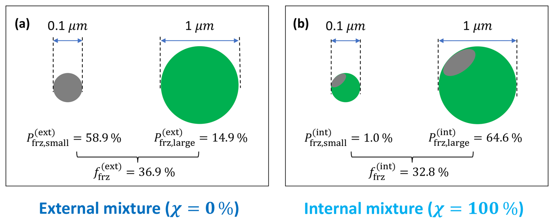
Figure E1 Illustration of a counterexample comparing external and internal mixing states for a polydisperse aerosol population consisting of particles with diameters of 0.1 and 1 µm. Gray denotes Fe₂O₃ (efficient ice-nucleating species) and green denotes illite (less efficient species). Freezing probabilities are evaluated under constant conditions of $T=-\mathrm{30}$ °C and a duration time of 3600 s. Panel (a) shows the externally mixed configuration, while panel (b) shows the internally mixed configuration with the same total surface area of each species.

Appendix F: Efficiency and exactness of the accelerated algorithm

In this appendix, the terms “naive algorithm” and “accelerated algorithm” refer to Algorithm 2 and Algorithm 3 in Sect. 4.3, respectively. Figure F1 compares the run time and efficiency gains for the naive and accelerated algorithms for the eight cases listed in Table 2. The performance metrics were obtained from 20 independent trials for each case, evaluating both algorithms separately. The run times reflect exclusively the immersion freezing process. Other aspects such as model initialization, file input/output operations, and simulations of other physical processes are excluded from this evaluation. All tests were conducted on a single core of the Keeling computer cluster at the University of Illinois at Urbana-Champaign.

The accelerated algorithm reduces the run time on average by 87.26 %, which is equivalent to a ×7.85 speed up.

In the context of the tau-leaping algorithm, when the simulation involves particles with less effective INPs, the majority of these INPs are bypassed during the tau-leaping steps. This suggests that the accelerated algorithm is more efficient in simulating the freezing process of particles with lower-efficiency INPs. However, since each particle can only undergo one freezing event before melting, and if the temperature remains below 0 °C, both the naive and accelerated algorithms will only account for particles that remain unfrozen. Particles containing more effective INPs exhibit a higher freezing ratio, resulting in fewer unfrozen particles. Consequently, as the algorithm iterates over a diminishing pool of unfrozen particles, the computational running time is reduced. Thus, simulating the freezing of particles with highly efficient INPs can lead to run-time efficiencies in this manner. These competing effects may partially account for the insignificant variations in run time reduction observed across different INP groups, as shown in the panel (b) of Fig. F1.

Figure F2 presents a comparison of the frozen fraction results simulated by the naive and accelerated algorithms. The outcomes from both algorithms are closely aligned, with a correlation coefficient exceeding 0.999 and a root mean square error (RMSE) of just 0.098 (expressed as a percentage). These minor discrepancies are entirely justifiable, considering the inherent stochastic variance expected from random algorithms and underscore the robustness of the accelerated algorithm.

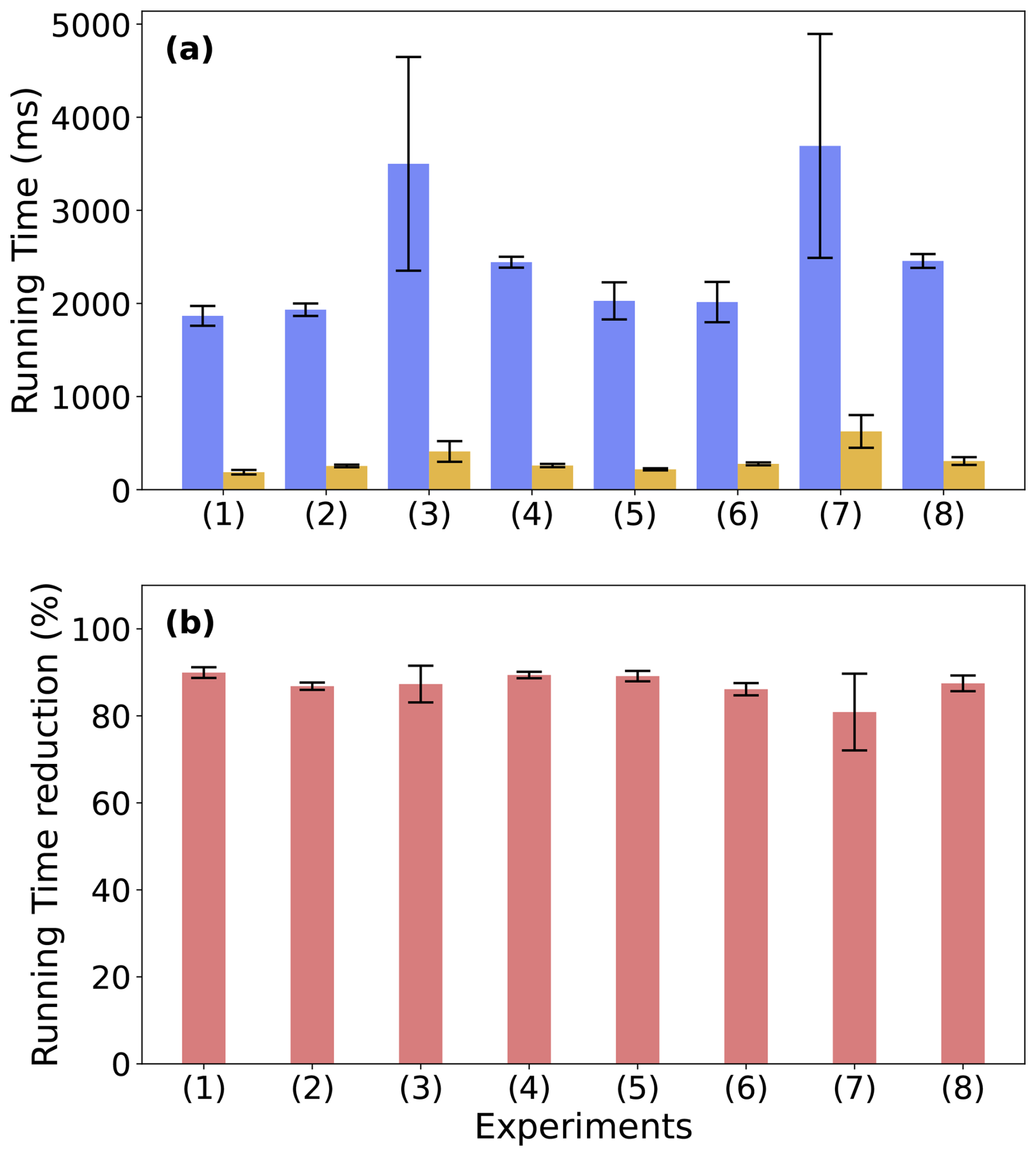
Figure F1 Runtime reductions for naive and accelerated algorithms. Panel (a) shows the running times of the naive (blue) and accelerated (orange) algorithms across eight different experiments. Panel (b) depicts the percentage of time reduction achieved by the accelerated algorithm in each run. Error bars represent the standard deviation of run times, indicating variability in simulation times across 20 trials.

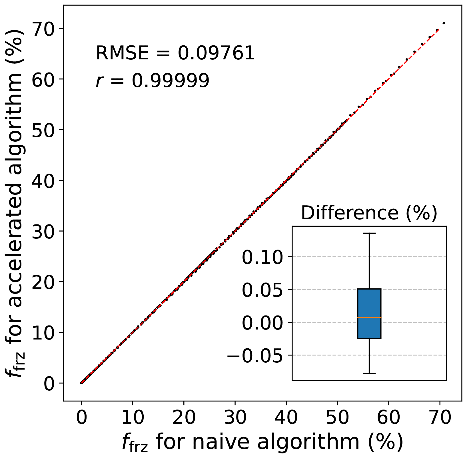
Figure F2 Average frozen fraction at 10 s intervals from eight experiments as obtained by the naive and accelerated algorithms. Each data point is the mean of 20 trials per experiment, showing the precision of the accelerated algorithm in simulating the freezing process. The red dashed line represents a one-to-one correlation. The inset boxplot illustrates the maximum, 75th percentile, median, 25th percentile, and minimum of the f_frz differences between the accelerated and naive algorithms.

The method of grouping particles into bins and the approach used to calculate the $P_i^{\text{max}}$ for each bin can significantly influence the algorithm's efficiency. If there is a large variance in the selection probability of particles within the same bin – meaning the upper bound value, $P_i^{\text{max}}$, is substantially higher than the selection probabilities for the majority of particles in that bin, the algorithm's efficiency decreases. This scenario occurs when factors other than particle size affect their selection probability.

In the context of immersion freezing simulations for single-species INPs, variations in freezing probabilities are solely due to size differences, as all INPs are of the same species and are exposed to the same environmental conditions. The PartMC model groups particles by size, ensuring that INPs within the same bin are similarly sized and, therefore, have comparable freezing probabilities. However, for externally mixed INP collections, such as Cases 3 and 7, to make sure $P_i^{\text{max}}$ is the upper bound of the freezing probability within the ith bin, it is calculated by $P_i^{\text{max}}=\mathrm{1}-\exp (-S_{\text{p,}i}^{\left(\text{max}\right)}\cdot J_{\text{het}}^{\text{(max)}}\cdot \mathrm{\Delta }t)$, where $S_{\text{p,}i}^{\left(\text{max}\right)}$ is the surface area of the largest particle over that bin, $J_{\text{het}}^{\text{(max)}}$ is the ice nucleation rate coefficient of the most efficient species, and Δt is the time interval during the simulation. This can lead to a large overestimation of the real freezing probability for INPs only covered by less efficient species within that bin. In the Cases 3 and 7, the algorithm selects many illite particles using the maximum freezing probability of Fe₂O₃ particle during tau-leaping, and then rejects most of them in the secondary selection. For example, in case 7 at 600 s, where the temperature is −30 °C, the ice nucleating rate coefficients are $J_{\text{het}}^{\left({\mathrm{Fe}}_{\mathrm{2}}{\mathrm{O}}_{\mathrm{3}}\right)}=\mathrm{7.85}\times {\mathrm{10}}^{\mathrm{9}}$ ${\mathrm{m}}^{-\mathrm{2}}{\mathrm{s}}^{-\mathrm{1}}$ and $J_{\text{het}}^{\left(\text{illite}\right)}=\mathrm{1.42}\times {\mathrm{10}}^{\mathrm{7}}$ ${\mathrm{m}}^{-\mathrm{2}}{\mathrm{s}}^{-\mathrm{1}}$. Consider the ith bin containing particles with dry diameters ranging from 1 µm to 1.1 µm, and assume Δt=1 s. The maximum freezing probability in this bin is $P_i^{\text{max}}=\mathrm{0.0294}$. However, the actual freezing probability for illite particles of 1 µm diameter is only $\mathrm{4.48}\times {\mathrm{10}}^{-\mathrm{5}}$–656 times smaller than $P_i^{\text{max}}$. This implies that, out of 100 000 unfrozen computational particles, the tau-leaping algorithm would initially select approximately 2940 particles, yet only 4 to 5 particles would remain after the secondary selection. This inefficient process increases the run time and results in a relatively lower run time reduction, as shown in Fig. F1. Even so, in Case 3 and Case 7, the binned tau-leaping algorithm still saved over 80 % of computation time on average compared to the naive algorithm. Using the binned tau-leaping algorithm remains a better choice. A potential solution to this issue is to group INPs by both size and modes, where we assume aerosols are internally mixed within each mode. This bin structure ensures that particles within each bin are of the same species and similar size. Consequently, the $P_i^{\text{max}}$ would not excessively exceed the probabilities of most particles in the bin, potentially enhancing the algorithm's overall efficiency. However, maintaining a two-dimensional bin structure would come with additional computational cost.

Appendix G: Definition of χ index with respect to surface

The definition of χ index with respect to species surface is defined in Table G1, while the mathematical signs are defined in Table D1. Definition is similar to that of Riemer and West (2013), the only difference is using the surface ratio instead of the mass fraction.

Table G1 Definitions of aerosol mixing entropies, particle diversities, and mixing state index. In these definitions we take 0ln 0=0 and 0⁰=1. The definition and naming of the quantities are based on Riemer and West (2013).

Appendix H: Method for generating the INP population with specific mixing state

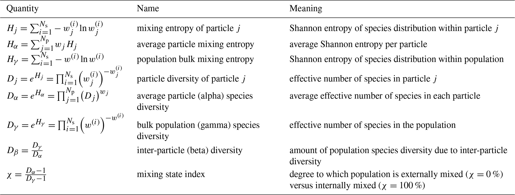
The objective of this method is to generate an INP population in which particles within each size bin exhibit an intermediate mixing state defined by a prescribed χ value. We begin by initializing two separate INP populations composed entirely of pure Fe₂O₃ and pure illite, respectively, both sharing the same size distribution. By combining these two populations, we obtain an externally mixed INP population with χ=0 %.

Next, we divide the combined population into 100 size bins. Within each bin, we iteratively introduce mixing as follows: two particles (e.g., particles j₁ and j₂) are randomly selected, and a surface area S_e is randomly generated from a uniform distribution between 0 and $min\mathit{\{}{S}_{{\mathrm{p}}_{j_{\mathrm{1}}}},S_{{\mathrm{p}}_{j_{\mathrm{2}}}}\mathit{\}}$. We then exchange this surface area between the two particles, assuming that the species surface ratio of the transferred surface segment from particle j₁ to particle j₂ is the same as species surface ratio of particle j₁, and the species surface ratio of the transferred surface segment from particle j₂ to particle j₁ is the same as species surface ratio of particle j₂.

This exchange process incrementally increases the degree of mixing within the bin, and consequently, the χ value. The selection and exchange steps are repeated until the χ value of the bin reaches the prescribed target. This procedure is applied independently across all bins, ensuring that particles within each bin attain the desired intermediate mixing state characterized by the specified χ.

Algorithm H1 summarizes the procedure described above. The mixing state is represented by a two-dimensional array $\mathbf{M}[\mathrm{1}:N_{\mathrm{s}},\mathrm{1}:N_{\mathrm{p}}]$, where M[i,j] denotes the fractional surface area of the jth particle covered by the ith species. Particle sizes are stored in a surface area array S_p[1:N_p], where S_p[j] corresponds to the surface area of the jth particle. The prescribed mixing state is defined by the target χ value, denoted as χ_obj.

Algorithm H1 Random surface exchange method (method of initializing an intermediate mixing state).

1:

Initializing an INP population Π with external mixture, each type of INP has the same size distribution

2:

Grouping Π to N_bin number of bins, ${\mathrm{\Pi }}_{\mathrm{1}},{\mathrm{\Pi }}_{\mathrm{2}},\mathrm{\dots },{\mathrm{\Pi }}_{N_{\text{bin}}}$.

3:

for $k=\mathrm{1},\mathrm{2},\mathrm{\dots },N_{\text{bin}}$  do

4:

loop

5:

Randomly select $j_{\mathrm{1}},j_{\mathrm{2}}\in {\mathrm{\Pi }}_k$

6:

r=randUnif ()

7:

$S_{\mathrm{e}}=r\cdot min\mathit{\left\{}{S}_{\mathrm{p}}\right[j_{\mathrm{1}}],S_{\mathrm{p}}[j_{\mathrm{2}}\left]\mathit{\right\}}$

8:

$\mathit{M}[:,j_{\mathrm{1}}]=\mathit{M}[:,j_{\mathrm{1}}]+\frac{\mathrm{1}}{S_{\mathrm{p}}\left[j_{\mathrm{1}}\right]}(-S_{\mathrm{e}}\cdot \mathit{M}[:,j_{\mathrm{1}}]+S_{\mathrm{e}}\cdot \mathit{M}[:,j_{\mathrm{2}}\left]\right)$

9:

$\mathit{M}[:,j_{\mathrm{2}}]=\mathit{M}[:,j_{\mathrm{2}}]+\frac{\mathrm{1}}{S_{\mathrm{p}}\left[j_{\mathrm{2}}\right]}(-S_{\mathrm{e}}\cdot \mathit{M}[:,j_{\mathrm{2}}]+S_{\mathrm{e}}\cdot \mathit{M}[:,j_{\mathrm{1}}\left]\right)$

10:

Calculate χ_k for Π_k.

11:

if χ_k≥χ_obj  then

12:

break

13:

end if

14:

end loop

15:

end for

Appendix I: Order-of-magnitude estimate of the computational particle number required to suppress sampling noise

For very low frozen fractions, sampling noise arising from the finite number of computational particles can become substantial. To estimate the computational particle number required to suppress this noise, we consider a confidence-interval-based approximation. Assume that, at a given time step, all unfrozen computational particles have the same freezing probability P_frz. Then the freezing of the unfrozen particles during that time step can be viewed as repeated Bernoulli trials, and the number of newly frozen particles satisfies

$$\begin{array}{}\text{(I1)}& \mathrm{\Delta }{N}_{\text{ice}}\sim \text{Binomial}(N_{\text{unf}},P_{\text{frz}}),\end{array}$$

where N_unf is the number of unfrozen computational particles at that time step. The corresponding estimator of the newly frozen fraction is $\widehat{p}=\mathrm{\Delta }{N}_{\text{ice}}/N_{\text{unf}}$. A rigorous confidence interval for $\widehat{p}$ may be constructed using the Clopper–Pearson exact interval. However, because that interval does not yield a simple closed-form expression for the required particle number, we use a normal approximation to obtain an order-of-magnitude estimate. When N_unf is sufficiently large, $\widehat{p}$ approximately follows

$$\begin{array}{}\text{(I2)}& {\displaystyle \frac{\mathrm{\Delta }{\widehat{N}}_{\text{ice}}}{N_{\text{unf}}}}\sim \mathcal{N}\left(P_{\text{frz}},{\displaystyle \frac{P_{\text{frz}}(\mathrm{1}-P_{\text{frz}})}{N_{\text{unf}}}}\right).\end{array}$$

Under this approximation, the half-width of a two-sided confidence interval at significance level α is

$$\begin{array}{}\text{(I3)}& z_{\mathrm{1}-\mathit{\alpha }/\mathrm{2}}\sqrt{{\displaystyle \frac{P_{\text{frz}}(\mathrm{1}-P_{\text{frz}})}{N_{\text{unf}}}}},\end{array}$$

where $z_{\mathrm{1}-\mathit{\alpha }/\mathrm{2}}$ is the corresponding standard-normal quantile. If one requires this half-width to be smaller than $\mathit{ϵ}\overline{f}$, where $\overline{f}$ denotes the characteristic magnitude of the frozen fraction of interest and ϵ is the prescribed relative tolerance, then a sufficient condition is

$$\begin{array}{}\text{(I4)}& z_{\mathrm{1}-\mathit{\alpha }/\mathrm{2}}\sqrt{{\displaystyle \frac{P_{\text{frz}}(\mathrm{1}-P_{\text{frz}})}{N_{\text{unf}}}}}\le \mathit{ϵ}\overline{f}.\end{array}$$

Rearranging gives

$$\begin{array}{}\text{(I5)}& N_{\text{unf}}\ge {\displaystyle \frac{z_{\mathrm{1}-\mathit{\alpha }/\mathrm{2}}^{\mathrm{2}}{P}_{\text{frz}}(\mathrm{1}-P_{\text{frz}})}{{\mathit{ϵ}}^{\mathrm{2}}{\overline{f}}^{\mathrm{2}}}}.\end{array}$$

For the very-low-frozen-fraction regime of interest here, we have N_unf≈N_p. Therefore, Eq. (I5) implies the order-of-magnitude estimate

$$\begin{array}{}\text{(I6)}& N_{\mathrm{p}}\gtrsim {\displaystyle \frac{z_{\mathrm{1}-\mathit{\alpha }/\mathrm{2}}^{\mathrm{2}}{P}_{\text{frz}}(\mathrm{1}-P_{\text{frz}})}{{\mathit{ϵ}}^{\mathrm{2}}{\overline{f}}^{\mathrm{2}}}}.\end{array}$$

Equation (I6) provides only an order-of-magnitude estimate, because it assumes a common freezing probability for all unfrozen particles within a time step and neglects correlations across time steps. For Case 1, the frozen fraction is on the order of $\overline{f}=\mathrm{0.001}\mathit{\%}={\mathrm{10}}^{-\mathrm{5}}$. Taking $P_{\text{frz}}\approx \overline{f}$, α=0.05 (95 % confidence interval), and ϵ=0.1, Eq. (I6) gives $N_{\mathrm{p}}\gtrsim \mathrm{3.8}\times {\mathrm{10}}^{\mathrm{7}}$. This estimate suggests that resolving frozen fractions at the level of Case 1 with a relative uncertainty of about 10 % would require on the order of 10⁷–10⁸ computational particles. For Case 2, the characteristic frozen fraction is on the order of $\overline{f}\sim \mathrm{0.1}$. Using the same values of α and ϵ gives $N_{\mathrm{p}}\gtrsim \mathrm{3.5}\times {\mathrm{10}}^{\mathrm{3}}$. Thus, using 10 000 computational particles is sufficient to suppress sampling noise in Case 2.