Two years of total column measurements of CO₂, CH₄ and CO in Paris, France

Several cities have established atmospheric monitoring networks to track greenhouse gas emissions. In the Paris metropolitan area, continuous in-situ surface measurements have been conducted since 2015. To complement them, three ground-based solar Fourier Transform Infrared (FTIR) spectrometers (Bruker EM27/SUN and Bruker IFS125HR) provide total column concentrations of CO₂, CH₄, CO, and H₂O (XCO₂, XCH₄, XCO, XH₂O): Jussieu (JUS, since 2014), Saclay (SAC, since 2021), and Gonesse (GNS, since 2022) within the ICOS Cities project.

These total column estimates capture background variability and urban plumes but are influenced by calibration, measurement noise, solar geometry, a priori profiles, and surface pressure. Accounting for these factors, overall uncertainties are estimated at 0.2 ppm for XCO₂, 1.2 ppb for XCH₄, and 2 ppb for XCO (EM27/SUN instruments). Inter-station gradients reveal the influence of the Paris emission plume, with typical XCO₂ gradients below 1 ppm (mean 0.51 ppm, 8.9 % above 1 ppm).

The observed XCO₂ gradients were compared with WRF-Chem simulations driven by the dynamic Origins.earth emission inventory. The correlations are moderate – 0.47 (SAC-GNS), 0.43 (JUS-GNS), and 0.26 (SAC-JUS) – with regression slopes of 0.66, 0.72, and 0.44, respectively, suggesting a potential overestimation of emissions by about 35 %. However, the large spread between measured and modelled gradients limits the robustness of this conclusion.

The paper first describes the monitoring network and harmonized data processing, then evaluates measurement uncertainties, and finally compares observations with model simulations to assess the potential of FTIR column data for validating urban emission inventories.

1 Introduction

Urban areas cover only about 3 % of the Earth's surface (Liu et al., 2014) but are home to 56 % of the world's population (World Bank, based on UN Population Division data, 2023) and account for roughly 70 % of global anthropogenic CO₂ emissions (IPCC, 2023). They are therefore central to understanding the evolution of greenhouse gas emissions driving climate change (Albarus et al., 2023). In this study, we present two years of total column measurements of CO₂, CH₄, and CO within and around Paris (column-averaged dry air mole fractions, denoted by X…). Carbon dioxide (CO₂) is the main anthropogenic greenhouse gas driving current climate change. It is produced primarily by the combustion of fossil fuels in human activities such as traffic, residential heating, and industry (Pachauri et al., 2015). In the Paris region, emissions are mainly linked to road transport and residential heating (AirParif, 2022, 2025). Methane (CH₄) is the second most important anthropogenic greenhouse gas. Although its atmospheric concentration is roughly 200 times lower than CO₂, its mass-based warming potential is about 30 times greater over a 100-year time horizon (IPCC, 2023). Globally, the dominant CH₄ sources are natural wetlands and agricultural activities (IPCC, 2023; Saunois et al., 2020). In the Paris area, the main sources are landfills, waste treatment facilities, wastewater treatment plants, and leaks from natural gas transmission networks (Defratyka et al., 2021; AirParif, 2025). Carbon monoxide (CO) is not a greenhouse gas, but a by-product of incomplete combustion. It is mainly emitted by human activities such as residential heating and road traffic. Unlike CO₂, biogenic sources of CO – apart from wildfires – are negligible, making it a useful tracer of anthropogenic emissions in interpreting concentrations of other species.

The Paris region currently operates a network of nine sites measuring CO₂, CH₄, and CO continuously from towers and rooftops and are used for estimates of the anthropogenic emissions through atmospheric inversions (Bréon et al., 2015; Staufer et al., 2016; Xueref-Remy et al., 2018; Lian et al., 2021; Lian et al., 2022; Nalini et al., 2022; Lian et al., 2023).

ICOS-Cities, a project supported by the European research infrastructure ICOS (Integrated Carbon Observation System), aims to develop systematic CO₂ observations in urban areas to monitor emission trends and provide tools and services for city administrations as part of their climate action plans. Three pilot cities have been selected in Europe:

• Paris, France (urban area: 12 million inhabitants)

• Munich, Germany (urban area: 2.4 million inhabitants)

• Zurich, Switzerland (urban area: 1.3 million inhabitants)

Paris, with its high population density, isolation from other major urban centers, and estimated CO₂-equivalent emissions of 37 Mt in 2021 (AirParif, 2025), is particularly well suited to studying the link between emissions and concentration gradients, and to developing methods for estimating emissions from atmospheric observations. Analyses of surface measurements have shown both potential and limitations, largely due to uncertainties in vertical mixing in atmospheric transport models (Bréon et al., 2015). Total column measurements can mitigate this issue by being less sensitive to vertical mixing errors, and they are also the quantity observed by satellites. The forthcoming CO₂M satellite, for example, is designed to monitor urban emissions based on CO₂ column imagery. There is thus a clear need to characterize CO₂ column variability around a large city such as Paris.

To this end, three Paris network stations, Saclay (SAC), Gonesse (GNS) and Jussieu in central Paris (JUS) have been equipped with Fourier Transform Infrared (FTIR) solar spectrometers to measure CO₂, CH₄, CO, and H₂O total columns. The instruments used in this study are:

• Bruker EM27/SUN (Frey et al., 2015, 2019; Alberti et al., 2022), a low-resolution FTIR spectrometer (0.5 cm⁻¹), in continuous operation at SAC and GNS since 2021 and 2022, respectively.

• Bruker IFS 125 HR, a high-resolution FTIR spectrometer (up to 0.02 cm⁻¹), operating at JUS since 2014 and part of the TCCON (Wunch et al., 2011) and NDACC (Sussmann et al., 2013; De Mazière et al., 2018) networks.

Meteorological data show that prevailing winds at 100 m above ground level in the Paris area are aligned along a north-east–south-west (NE–SW) axis (23 % SW and 13 % NE). This motivated the choice of SAC (SW) and GNS (NE) for FTIR column measurements during ICOS-Cities, as these sites are ideally positioned upwind and downwind of the city. When the wind blows from either direction, the observed gradients provide direct information on city emissions and can be used to estimate them through the differential column measurement (DCM) method (Chen et al., 2016).

The aim of this study is to conduct a detailed analysis of CO₂ column measurements, characterize variations linked to surface fluxes, and compare them with atmospheric modelling to assess the contribution of column observations to urban emission estimates. Throughout the paper, CO₂ columns are referred to as XCO₂, which includes vertical weighting effects as discussed in Sect. 3.3.

Studies based on CO₂ total column measurements have already been conducted in several major urban areas worldwide. In 2015, a pilot campaign was carried out in Paris (Vogel et al., 2019) using five low-resolution FTIR spectrometers deployed in and around the city for one month in the spring. These measurements revealed spatial XCO₂ gradients of 1–1.5 ppm. Coupled with CHIMERE simulations, the analysis showed that anthropogenic emissions dominated the gradients, although biogenic fluxes also contributed during periods of strong vegetation activity. In the Paris area, numerical simulations suggest that biogenic fluxes can generate station-to-station XCO₂ differences of up to 1 ppm in spring. For a few selected days, correlations between measured and modelled gradients ranged from 0.8 to 0.96, indicating that accurate FTIR measurements can support emission estimates for large cities.

In Europe, similar campaigns have been conducted in Munich (Dietrich et al., 2021; Zhao et al., 2023), Thessaloniki (Mermigkas et al., 2021), Madrid (Tu et al., 2022), and Berlin (Hase et al., 2015; Zhao et al., 2019). In Munich, a permanent network of five EM27/SUN instruments operates continuously, with one in the city center and four surrounding the city on a 10 km radius. The measurements show a steady increase of 2.4 ppm yr⁻¹, although urban–background gradients (0.5–1 ppm) are smaller than those in Paris, reflecting Munich's smaller size and lower population density. In Berlin, a 2014 campaign with five spectrometers (Hase et al., 2015) revealed a city emission signal of ∼ 1 ppm. Using a very simple dispersion model, emissions were estimated at ∼ 800 kgCO₂ s⁻¹, 20 % to 45 % higher than reported emission inventories (545 kgCO₂ s⁻¹ in 2019; 675 kgCO₂ s⁻¹ in 2010). However, Zhao et al. (2019) found a relatively poor agreement between FTIR measurements and WRF-GHG simulations (Weather Research and Forecasting modeled coupled with a GreenHouse Gas module).

Outside Europe, similar efforts include Indianapolis (Jones et al., 2021), Mexico City (Che et al., 2024), Beijing (Che et al., 2022), St. Petersburg (Ionov et al., 2021), and Tokyo (Ohyama et al., 2023). Mexico City, with about twice the population of Paris but similar CO₂ emissions, hosted a 2020–2021 campaign with seven FTIR instruments, including one NDACC high-resolution site in continuous operation since 2012 (Altzomoni Atmospheric Observatory). Gradients of 1–1.5 ppm were observed at the most urbanized sites, comparable to Paris in 2015. In cities with stronger emissions, such as St. Petersburg and Tokyo, plume signatures are much larger – up to 4.5 ppm in St. Petersburg and 9.5 ppm in Tokyo. Notably, in St. Petersburg, column measurements suggested emissions three times higher than the city's reported inventory (Ionov et al., 2021).

These studies demonstrate that total column measurements can, in some cases, be used to optimize emission inventories, particularly where a priori inventories contain large uncertainties. However, weak correlations between measurements and simulations in cities with lower emissions indicate that the method is only effective when urban signals are strong enough.

The establishment of a permanent measurement network, the production of a multi-year CO₂ column time series in a densely populated urban area, and the use of WRF-Chem (WRF model coupled with an atmospheric Chemistry module) with a dynamic emission inventory together provide a unique opportunity to evaluate the potential of total column observations to validate urban emission inventories.

In the following sections, we first present the instrument network used to measure greenhouse gas columns in the Paris region. We then demonstrate how to disentangle instrumental effects from geophysical variability in the observed time series. Finally, we compare measured columns with WRF-Chem simulations to assess the extent to which such observations can help refine the Origins.earth emission inventory used as a priori input for the model.

2 Presentation of the column measurement network in the Paris' urban area

2.1 Stations and instruments deployed in and around Paris

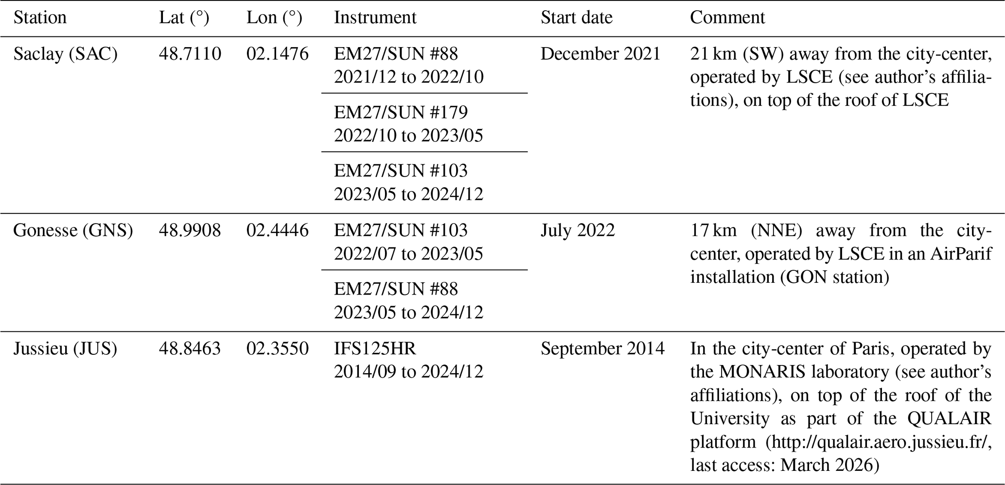
Of the nine stations composing the Paris in-situ greenhouse gas monitoring network in 2025, three are equipped with FTIR spectrometers for measuring total columns. The first (JUS) has been operating since 2014, while the most recent (GNS) began in July 2022 (see Table 1). SAC started in between, in December 2021. These three stations provide a time series of more than 10 years, including two years and a half common to all stations.

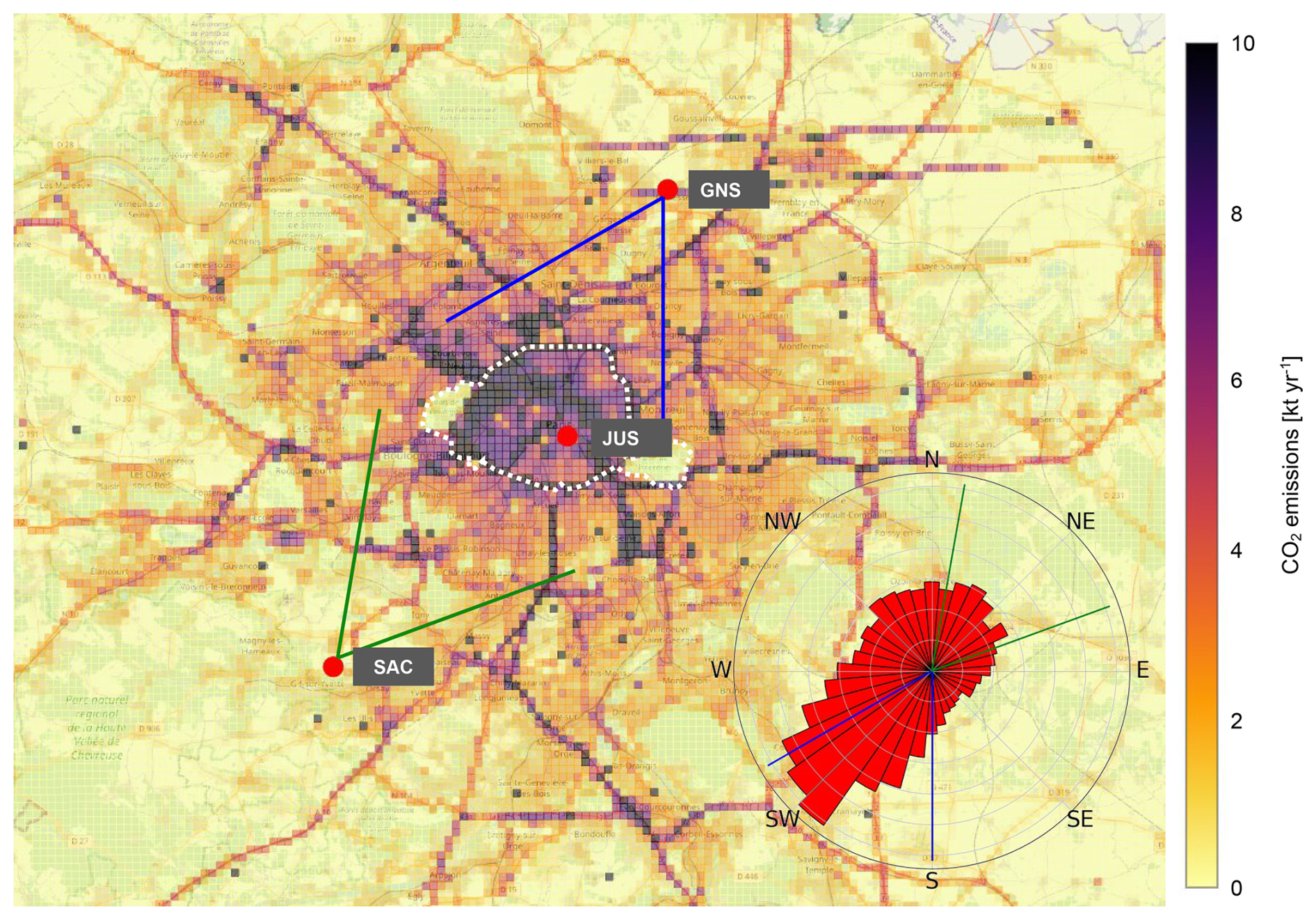
Figure 1 Map of the column measurements network in the Paris' region. The three stations are arranged along the axis of the prevailing wind as shown on the polar plot of the wind directions between 2014 and 2024 (included). The green and blue lines show the wind direction sectors representative of the airmasses coming from Paris to SAC and GNS respectively. The white dotted line denotes the administrative boundary of the Paris city. The map shows the total CO₂ emissions in 2019 (Data source: official AirParif emission inventory).

Figure 1 shows the location of the three FTIR sites, aligned along the prevailing wind axis (approximately NE–SW) characteristic of the Paris region and much of Western Europe. The polar plot displays the distribution of wind directions at Saclay (100 m above ground level) calculated over the 2014–2024 period, which is representative of regional winds. These measurements are used to define upwind–downwind gradients between stations, reflecting surface-atmosphere fluxes across the intervening urban area. This approach, known as Differential Column Measurements (DCM), is described in Chen et al. (2016) and Dietrich et al. (2021). Only gradients associated with the selected wind sectors (green and blue in Fig. 1) are analysed in Sect. 5.

Table 1 Stations used for total column measurements in the Paris' network.

The EM27/SUN spectrometers at all three sites are automated using dedicated enclosures designed at LSCE. Each enclosure is equipped with a direct sunlight sensor and a rain sensor, which trigger the automatic opening of the hood and start-up of the CamTracker (Gisi et al., 2011) and OPUS (Bruker Users Manual, Bruker, 2026) measurement software. For the JUS site, the IFS 125 HR measurement automation is designed and developed by MONARIS and is effective since June 2024.

In addition, each system includes a calibrated Vaisala PTU300 probe for continuous pressure measurements, ensuring accurate data processing (see Sect. 2.2). A travelling EM27/SUN is also used for side-by-side comparisons (Sect. 2.3) and scale transfer.

2.2 Data processing

Data processing, from raw interferograms of the EM27/SUN spectrometers to final total column estimates, is performed with PROFFAST v2.3 and PROFFASTpylot v1.2, developed and maintained at Karlsruhe Institute of Technology (KIT). More details can be found in Herkommer et al. (2024) and Feld et al. (2024). At LSCE, these tools run on a dedicated server, complemented by an overlay system designed to automate and parallelize processing for about a dozen EM27/SUN instruments. This workflow enables quasi-near-real-time processing, allowing rapid identification of instrumental issues and maximizing data completeness. Between versions 2.3 and 2.4 of PROFFAST, the XCO₂ estimates differ, on average, by −0.03 ppm with some dispersion around this mean value: 90 % of the XCO₂ differences are between −0.08 and 0.03 ppm. There are a few outliers (up to 0.4 ppm) but we have not been able to identify how these outliers differ from the typical case. The XCO₂ differences (between the two versions) of PROFFAST are correlated between the two ICOS stations so that the dispersion in term of ΔXCO₂ is lower than the dispersion on XCO₂. Indeed, 90 % of the ΔXCO₂ changes (between two versions of PROFFAST) are between −0.03 and 0.03 ppm. These differences are relatively small in comparison to the other sources of errors. They are therefore neglected in the following.

PROFFAST was originally developed to incorporate a priori atmospheric profiles from the GGG2014 and then the GGG2020 model (Laughner et al., 2023), used by the TCCON community with the GGG/GFit retrieval. The LSCE overlay software also allows retrievals using CAMS (Copernicus Atmospheric Monitoring System) forecast atmospheric profiles as a priori atmospheric profiles (Agustí-Panareda et al., 2014; Tang et al., 2018). Thus, for each measurement, two parallel datasets are produced: one using GGG2020 model and another using CAMS forecast. Differences between the two are analysed in Sect. 3.5.

As part of the PAUL project (Pilot Application in Urban Landscapes, also know as ICOS-Cities), LSCE's automated chain was validated by cross-processing a raw dataset with the MUCCnet group from the Technical University of Munich (TUM). Comparison of final datasets (both using GGG2014 a priori) showed no significant differences between the two groups.

Within the NUBICOS (New Users for a Better ICOS, a project that aims to strengthen ICOS procedures and improve value generation from observations) Horizon-Infra project, total columns retrieved from EM27/SUN are also integrated into the ICOS database, along with surface pressure records. This integration enables use of ICOS tools for quality control and visualization, while also ensuring long-term traceability (Hazan et al., 2016).

Jussieu total column measurements from IFS 125 HR instrument are processed using the retrieval software GGG2020 package (GGG2020 a priori profiles, GFit retrieval code, post-processing, see Laughner et al., 2024) and distributed through the TCCON archive (https://tccondata.org, last access: March 2026). This involves using the GFit retrieval algorithm to calculate columns with profiles generated by GGG2020 (unlike EM27/SUN data processing, which uses PROFFAST with GGG2020 a priori profiles).

2.3 Data availability at the three sites

The completeness of solar FTIR column time series strongly depends on weather conditions. The automated enclosures maximize data acquisition by exploiting short clear-sky intervals, reducing the need for manual operation.

Data availability is evaluated monthly as:

$$\begin{array}{}\text{(1)}& A=\mathrm{100}\cdot N_{\mathrm{MesDays}}/N_{\mathrm{AllDays}}\end{array}$$

where N_MesDays is the number of days with valid measurement data and N_AllDays is the total number of days in the month.

Data availability at the three stations, along with clear-sky fraction (CSF) from the nearest Météo France site, are shown in Fig. S1 in the Supplement. As expected, availability is highly seasonal, from ∼ 10 %–20 % in winter to 70 %–80 % in summer, occasionally exceeding 85 % under favourable conditions. The gap at Gonesse between November 2022 and January 2023 is due to instrument failure.

At Jussieu, the situation differs: before automation of the high-resolution spectrometer in May 2024, it was operated manually, leading to lower data availability – typically 5 %–15 % in winter and ∼ 40 % in summer. Additional interruptions occurred due to technical failures in winter 2022–2023, spring 2023, and summer 2024.

3 Data quality and representativeness

3.1 Side-by-side comparisons

Total-column measurements in the Paris region are used to compute spatial gradients (see Sect. 5). Network consistency is therefore essential. We regularly perform side-by-side comparisons at each site using a travelling/mobile EM27/SUN as a common reference. These exercises ensure network-wide consistency and help detect potential instrumental drifts, which can be corrected by applying adjustment factors.

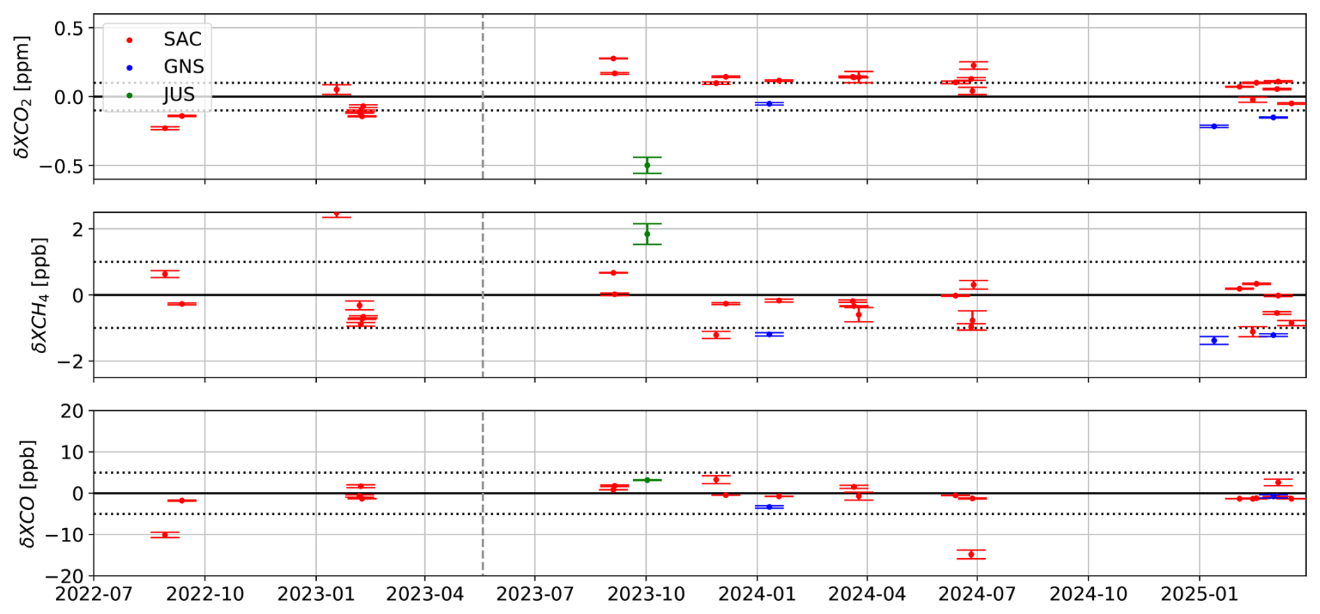
Figure 2 Daily means and uncertainties (see text) of XCO₂, XCH₄ and XCO side-by-side comparisons of each instrument with a mobile reference EM27/SUN. Notation δ is the differences between local instruments and mobile instrument estimates. The vertical grey dotted line corresponds to the date on which the two instruments were exchanged between the SAC and GNS stations.

Figure 2 reports daily means and uncertainties of XCO₂, XCH₄, and XCO for each instrument relative to the mobile reference EM27/SUN. Let δ denote the difference between a fixed station and the mobile reference. For each comparison day, we first smooth minute data with a 20 min rolling average, then compute the mean σ and standard deviation of the differences (σ). The uncertainty is given by:

$$\begin{array}{}\text{(2)}& \mathrm{Unc}={\displaystyle \frac{\mathit{\sigma }}{\sqrt{N}}}\end{array}$$

with:

• σ, the standard deviation

• N, the number of data

Comparisons are conducted on a regular basis, few times per year at Saclay. Logistical constraints delayed Gonesse comparisons until early 2024. Before 19 May 2023, instrument #88 was at Saclay and #103 at Gonesse; following which the two were exchanged. Because Saclay comparisons can be done on the LSCE laboratory rooftop, they are more frequent than at Gonesse, which requires a field visit.

The travelling instrument serves as a reference frame, but shall not be considered as absolute truth. Over the full period, XCO₂ side-by-side comparisons indicate good stability at both stations, with a bias lower than about 0.15 ppm between 2023 and 2024. We also find very good consistency for methane (<1 ppb) and carbon monoxide (∼ 1–2 ppb). This supports using both stations without additional corrections when computing regional gradients. A side-by-side comparison with the IFS 125 HR was carried out in October 2023 in Jussieu. These measurements show a bias of 0.5 ppm of XCO₂ on the comparison day (with an uncertainty of around 0.1 ppm), as well as 1.9 ppb (uncertainty around 0.5 ppb) of XCH₄ and 4 ppb (uncertainty around 1 ppb) of XCO.

3.2 Measurement's noise

The main source of observed short-term variability in EM27/SUN XCO₂ is instrumental noise. We quantify this using minute data smoothed with a 20 min rolling average. For each day we compute the standard deviation of the residuals to that smoothed series.

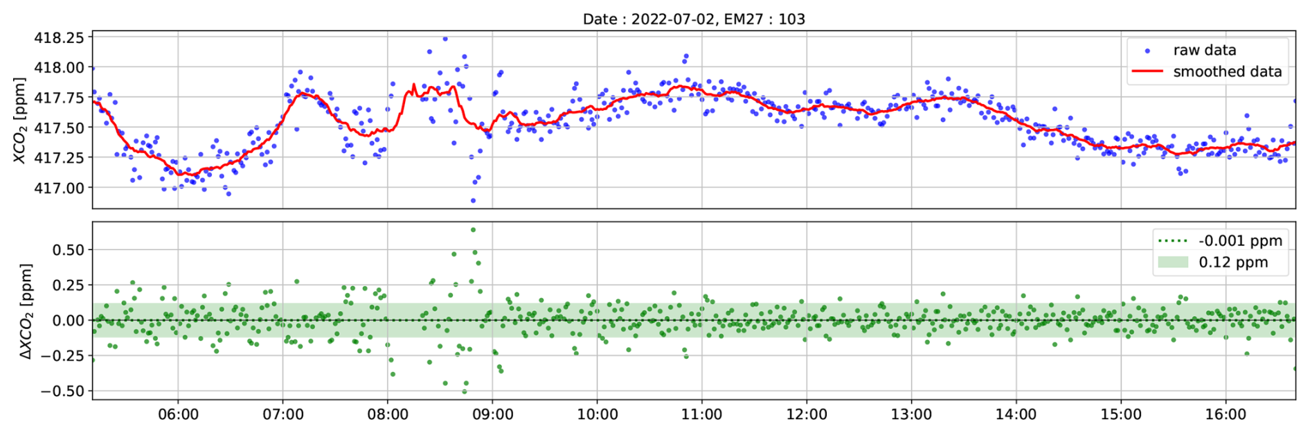
Figure 3 Example of a one day time series of XCO₂ measurements. The dots are the individuals measurements. The red line is the result of a 20 min smoothing. The bottom figure shows the difference between the individual measurements and the smoothed time series as weel as the standard deviation of these differences over the day (colored strip).

Figure 3 illustrates a sunny-day example at Gonesse: raw XCO₂ (blue), 20 min smoothing average (red), and residuals (bottom panel). For that day, the noise is estimated to be 0.12 ppm. Applying the same method to all instruments and their full records yields stable noise levels of ∼ 0.12 ppm (XCO₂), 0.6 ppb (XCH₄), and 0.4 ppb (XCO), in agreement with Gisi et al. (2012). We find no significant differences among EM27/SUN instruments. These values are shown by black dotted lines in Fig. S2. The Jussieu IFS 125 HR usually alternates between NDACC and TCCON measurements. Since we only use TCCON measurements, days with more than 200 spectra are fewer than in Saclay and Gonesse. On those days, using the exact same method than for EM27/SUNs, we estimate 0.55 ppm for XCO₂, 2.9 ppb for XCH₄, and 0.7 ppb for XCO; these estimates are indicated as a red dotted line in Fig. S2. For XCO, we exclude the EM27/SUN instrument #88 and report values representative of #103 and #179 only, because #88 exhibits an abnormally high average XCO noise (4.9, up to 10 ppb on some days), due to a known technical issue unresolved despite Bruker investigations.

3.3 Averaging kernel

EM27/SUN and IFS 125 HR record the solar spectrum after atmospheric transmission. Column retrievals are sensitive to the vertical distribution of absorbers because absorption varies with pressure and temperature. This vertical weighting is captured by the averaging kernel (AK), which depends on the species, the spectral windows, solar zenith angle (SZA), and instrument characteristics.

Figure S3 shows typical AKs for XCO₂, XCH₄, and XCO. For CO₂ and CH₄, EM27/SUN sensitivity is close to unity across most of the atmosphere at low SZA. At high SZA the sensitivity is enhanced in the lower troposphere. For CO, the sensitivity varies less with SZA and remains close to unity up to ∼ 200 hPa. Consequently, retrieved columns exhibit SZA-dependent behaviour (Sect. 3.4).

3.4 Variations due to the Solar Zenith Angle (SZA)

At Paris' latitude in summer, SZA spans ∼ 25–90°, offering a test for systematic SZA-related biases, especially at low elevations where path length and Earth curvature matter. For each day with sufficient data, we define the mean XCO₂ over the 10:00–14:00 local time as a reference (SZA < 50°). We then compute differences between minute-scale XCO₂ and that reference. We only consider days with noon SZA < 50° (spring–summer) and assume no large geophysical trend between midday and early/late hours.

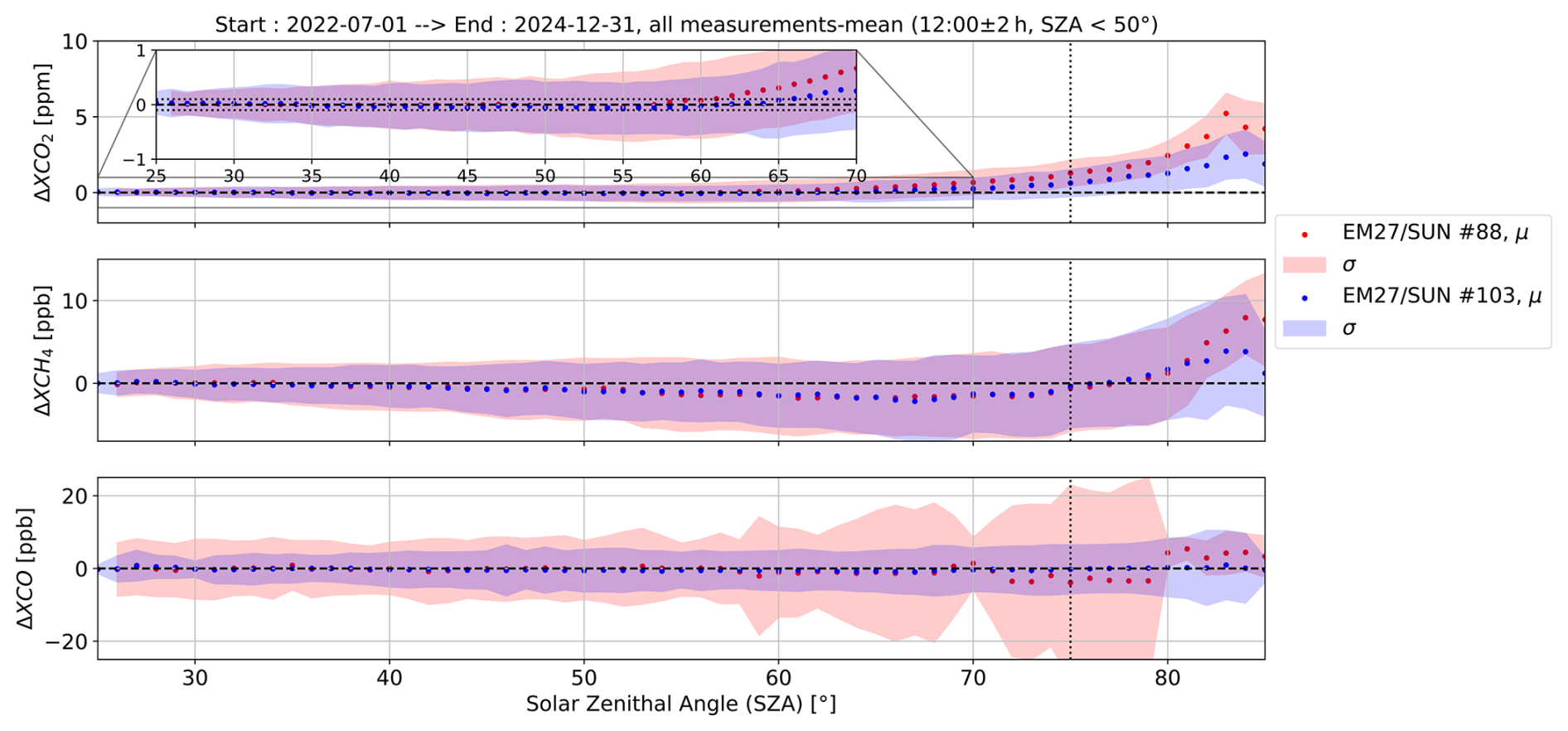
Figure 4 Differences between raw measurements and means of the 10 am–2 pm window when SZA < 50°, as a function of the solar zenith angle, from 1 July 2022 to 31 December 2024. The small panel is a zoom in the full one. The shaded area indicates the standard deviation of the individual differences for SZA bins of 1°.

Figure 4 reports mean differences versus SZA (bins of 1°) from 1 July 2022 to 31 December 2024 for instruments #88 and #103 (in Saclay and Gonesse); the shaded band shows the standard deviation in each SZA bin. Standard deviations increase with SZA, reflecting both increasing time from noon and genuine variability. Typical spreads are a few tenths of a ppm (XCO₂), ∼ 1 ppb (XCH₄), and a few ppb (XCO), confirming high precision.

We detect no systematic drift up to ∼ 60°. Beyond ∼ 65–70°, a drift emerges that grows with SZA and differs by gas: for XCO₂, it becomes noticeable above ∼ 75° (> 1 ppm) and reaches up to 3.5 ppm for 80-85°; for XCH₄, it remains smaller (<2 ppb up to 80°, up to 5 ppb between 80–85°); for XCO, it is negligible. The two instruments show consistent drifts, suggesting a primarily SZA-driven effect that is linked to poorly modelled radiative processes, with minor instrument-specific modulation (Tu, 2019).

3.5 Sensitivity to the a priori profile

PROFFAST uses a priori vertical profiles for CO₂, CH₄, CO, and H₂O, along with temperature and pressure, and retrieves columns by scaling the profiles to minimize the spectrum residuals. Because the a priori shapes differ, retrievals can be profile-dependent. We have compared the retrievals obtained with two different a priori from the GGG2020 and CAMS models, using the following equation:

$$\begin{array}{}\text{(3)}& X_{\mathrm{GAS}}=\mathrm{0.2095}.{\displaystyle \frac{{\mathrm{Column}}_{\mathrm{GAS}}}{{\mathrm{Column}}_{{\mathrm{O}}_{\mathrm{2}}}}}\end{array}$$

with:

• X_GAS, the measured GAS total column [in ppm or ppb]

• 0.2095, the mole fraction of O₂ in the ambient air

• Column_GAS, the GAS column [in molecules m⁻²]

• Column${}_{{\mathrm{O}}_{\mathrm{2}}},$ the O₂ column [in molecules m⁻²]

We evaluate the impact of the a priori vertical profile by comparing retrievals using CAMS versus GGG2020 a priori at Saclay and Gonesse (see Fig. 5). The x-axis shows differences between columns computed from the a priori only (see Eq. 4a to 4c). The y-axis shows differences between retrieved columns using PROFFAST and EM27/SUN measurements (see Eq. 3). The CAMS and GGG2020 columns used for the x-axis of Fig. 5 are computed by integrating the a priori profile (i.e. C^profile=C^prior), using the following equation:

$$\begin{array}{}\text{(4a)}& {\displaystyle }{X}_{\mathrm{GAS}}^{\mathrm{comp}}={\displaystyle \frac{{\sum }_i[C_i^{\mathrm{prior}}+{\mathrm{AK}}_i\cdot (C_i^{\mathrm{profile}}-C_i^{\mathrm{prior}}\left)\right]\cdot \mathit{\delta }{P}_i}{{\sum }_i\mathit{\delta }{P}_i}}\text{(4b)}& {\displaystyle }\leftrightarrow X_{\mathrm{GAS}}^{\mathrm{comp}}={\displaystyle \frac{{\sum }_i[{\mathrm{AK}}_i\cdot C_i^{\mathrm{profile}}+(\mathrm{1}-{\mathrm{AK}}_i)\cdot C_i^{\mathrm{prior}}]\cdot \mathit{\delta }{P}_i}{{\sum }_i\mathit{\delta }{P}_i}}\text{(4c)}& {\displaystyle }\leftrightarrow X_{\mathrm{GAS}}^{\mathrm{prior}}={\displaystyle \frac{{\sum }_i{C}_i^{\mathrm{prior}}\cdot \mathit{\delta }{P}_i}{{\sum }_i\mathit{\delta }{P}_i}}\end{array}$$

with:

• $X_{\mathrm{GAS}}^{\mathrm{comp}}$, the GAS total column computed from a given GAS profile (in-situ measurement, simulation)

• $X_{\mathrm{GAS}}^{\mathrm{prior}}$, the GAS total column computed from the a priori profile only

• AK_i, the GAS averaging kernel at level i

• $C_i^{\mathrm{prior}}$, the a priori GAS concentration at level i

• $C_i^{\mathrm{profile}}$, the GAS concentration in the measured or simulated profile (in which we compute the column) at level i

• δP_i, the pressure thickness of layer i

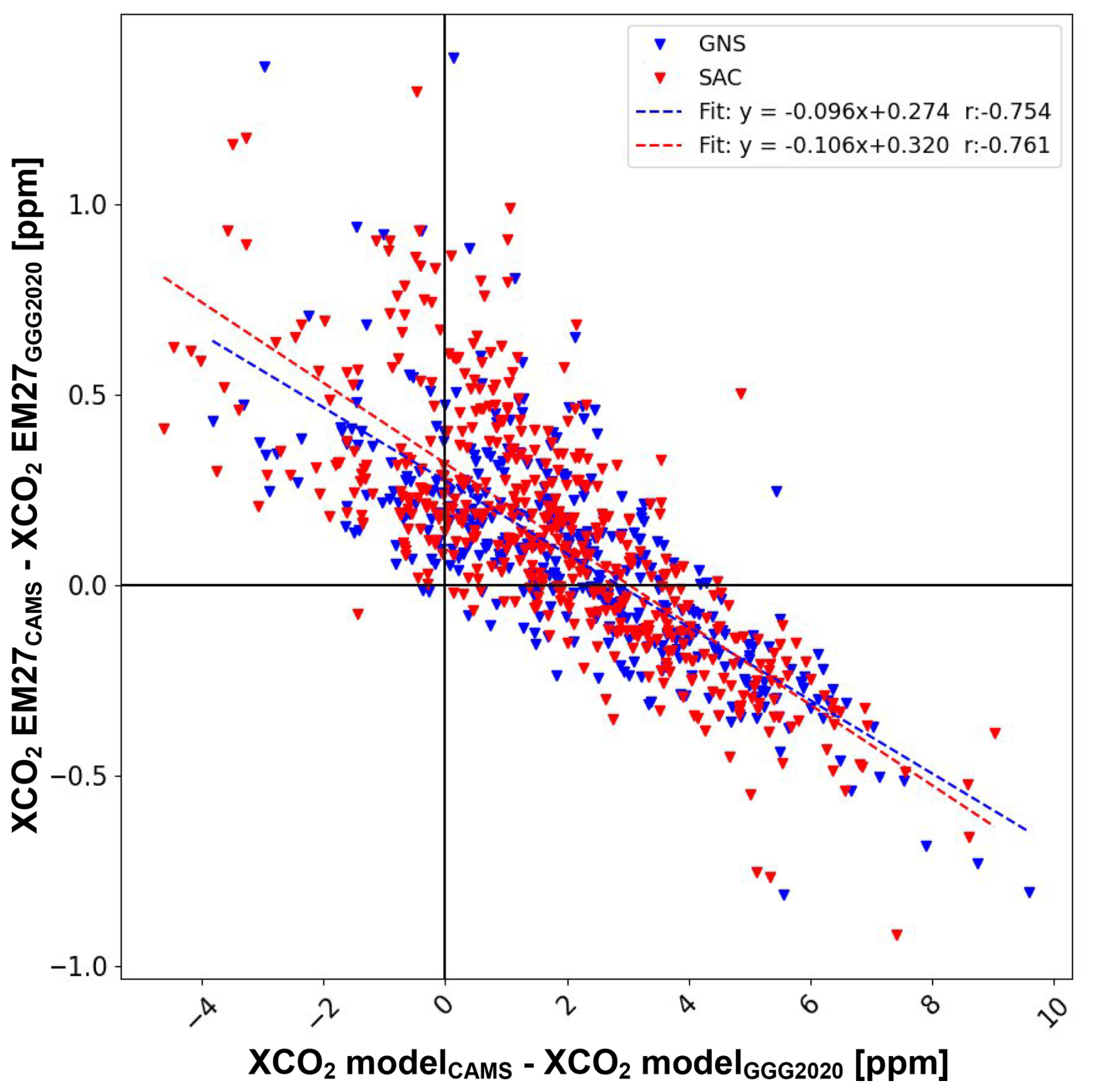
Figure 5 Differences between EM27/SUN CO₂ columns computed using the CAMS and GGG2020 a priori profiles as a function of the differences between columns computed from CAMS and GGG2020 a priori profiles only.

For both stations, the data points show a linear correlation ($r_{\mathrm{SAC}}=-\mathrm{0.76}$ et $r_{\mathrm{GNS}}=-\mathrm{0.75}$), indicating a systematic sensitivity of the retrievals to the a priori profile. The slope of the best linear fit is small (−0.11 at Saclay and −0.10 at Gonesse) and consistent between the two sites. We conclude that the EM27/SUN estimates using the PROFFAST retrieval tool shows some sensitivity to the a priori profile, which is independent of the station. The negative slope is physically consistent: most CAMS–GGG2020 differences occur in the lower troposphere, where GGG2020 (climatology) lacks synoptic variability. In those layers, AK > 1 (slightly), so (1 −AK) <  0; thus, increasing the a priori can decrease the retrieved column (see Eq. 4b).

Since the a priori profiles used for the estimates are very similar for the two sites (at a given time), this sensitivity has a negligible impact on the measured station-to-station gradient.

3.6 Sensitivity to the ground pressure measurements

Surface pressure is required by PROFFAST's radiative transfer and column scaling. Between 29 August 2024 and 31 January 2025, the Gonesse pressure sensor suffered a mechanical glitch (0 to 3 hPa bias, with short-term variability). We therefore re-processed the affected spectra using an alternate station 2 km away, altitude-corrected, which allows quantifying retrieval sensitivity to surface-pressure error. The altitude's correction being mostly constant, it allows us to correct the pressure data with no additional uncertainty.

We diagnose consistency with X_AIR, derived from O₂ absorption and expected to be near 1 (Frey et al., 2019):

$$\begin{array}{}\text{(5)}& X_{\mathrm{AIR}}={\displaystyle \frac{\mathrm{0.2095}}{m_{\mathrm{air}}\cdot {\mathrm{Column}}_{{\mathrm{O}}_{\mathrm{2}}}}}\left({\displaystyle \frac{P_{\mathrm{surf}}}{g}}-{\mathrm{Column}}_{{\mathrm{H}}_{\mathrm{2}}\mathrm{O}}\cdot m_{{\mathrm{H}}_{\mathrm{2}}\mathrm{O}}\right)\end{array}$$

Where:

• 0.2095, the mole fraction of O₂ in the atmosphere

• m_air, the molecular mass of dry air

• Column${}_{{\mathrm{O}}_{\mathrm{2}}},$ the O₂ column derived from spectra

• P_surf, the measured surface atmospheric pressure

• g, the gravitational acceleration at the surface

• Column${}_{{\mathrm{H}}_{\mathrm{2}}\mathrm{O}},$ the H₂O column derived from spectra

• $m_{{\mathrm{H}}_{\mathrm{2}}\mathrm{O}},$ the molecular mass of water vapor

In theory, the X_AIR parameter is equal to 1, as it represents the ratio between the measured dry air column and the expected dry air column, based on well-known atmospheric constant (most notably the fixed molar fraction of molecular oxygen (O₂) in dry air, which is approximately 20.95 %).

In practice, X_AIR deviates slightly due to calibration/ILS (Instrumental Line Shape), surface-pressure or altitude errors, local atmospheric variability (e.g., clouds), O₂ spectroscopy uncertainties, and time stamp error on the recorded spectra. An empirical tolerance of $\pm \mathrm{4}\cdot {\mathrm{10}}^{-\mathrm{3}}$ around 1 is typically accepted; larger deviations lead to rejection of the measurements. Note that $\mathrm{4}\cdot {\mathrm{10}}^{-\mathrm{3}}$ in X_AIR corresponds to ∼ 0.37 ppm in XCO₂ according to the results shown in Table 2.

Differences between columns before/after pressure correction are linearly proportional to the applied pressure offset (r≥0.99 for all species). The sensitivities are summarized in Table 2.

Table 2 Sensitivities of the XCO₂, XCH₄, XCO and X_AIR column measurements to the measured ground pressure for EM27/SUN measurements.

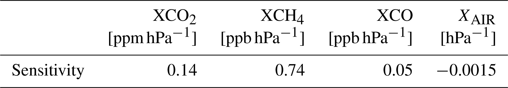
These values closely match Tu (2019). To keep systematic XCO₂ errors below 0.05 ppm, surface-pressure biases must therefore be lower than 0.3 hPa.

3.7 Estimating an uncertainty of column measurements in the Paris' network

The subsections above identify the dominant sources of error and sensitivities for EM27/SUN and IFS 125 HR total-column retrievals in dense urban and peri-urban environments. We group them as:

• Random error: measurement noise (short-term, no reproducible temporal pattern).

• Instrument-specific systematic error: calibration bias/drift between calibrations (electronics/optics).

• SZA sensitivity: spectroscopic/geometry-driven bias, largely instrument-independent.

• Vertical-distribution (AK) sensitivity: spectroscopic weighting; treated as instrument-independent.

• A priori dependence: inversion-related systematic, small and similar across EM27/SUN; not assessed for IFS 125 HR here.

• Surface-pressure dependence: linear scaling of column error with pressure error.

Since the overall uncertainty on the column retrievals arises from several statistically independent error sources, it can be estimated by quadratically combining the individual contributions (calibration and noise), as follows:

$$\begin{array}{}\text{(6)}& {\mathit{\sigma }}_{\mathrm{tot}}=\sqrt{{\sum }_i{\mathit{\sigma }}_i^{\mathrm{2}}}\end{array}$$

where σ_i denotes the typical values of the independent error sources. All results are summarized in Table 3.

Table 3 Error sources and sensitivities in the columns' measurements of the Paris network for each instrument (EM27/SUN and IFS 125 HR).

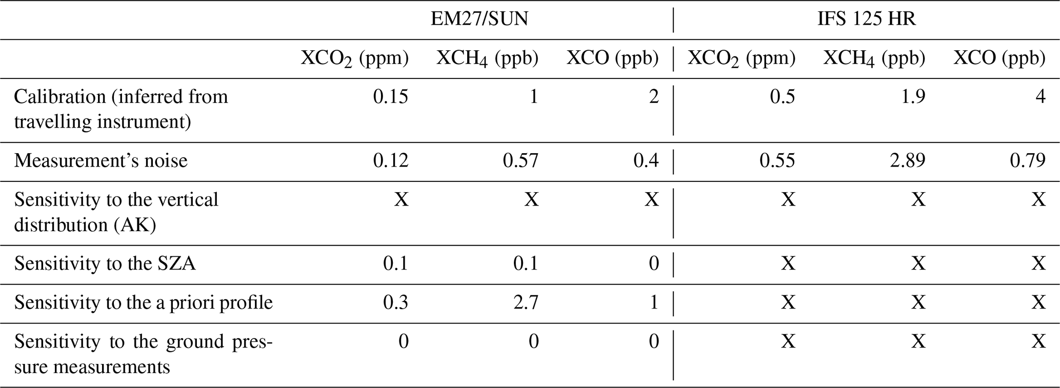
For EM27/SUN, we estimate global errors (from the calibration and noise contributions) of ∼ 0.2 ppm for XCO₂, ∼ 1.2 ppb for XCH₄, and ∼ 2 ppb for XCO on raw EM27/SUN columns and ∼ 0.7 ppm for XCO₂, ∼ 3.5 ppb for XCH₄, and ∼ 4.1 ppb for XCO on IFS 125 HR columns.

4 Geophysical variations of column measurements in the Paris' urban area

The objective of this section is to analyze the temporal variability of column-averaged CO₂, CH₄, and CO concentrations retrieved with PROFFAST (with CAMS a priori profiles) from EM27/SUN and GGG2020 for TCCON spectra. A thorough understanding of the geophysical drivers of variability is essential for using these measurements to estimate city-scale emissions.

4.1 Synoptic to seasonal scale variations

The time series exhibit variability at multiple timescales - weeks, months, and years. Figure 6 shows XCO₂ time series at Saclay, Gonesse, and Jussieu between 1 July 2022 and 31 December 2024. Colors indicate individual instruments, while the black solid line represents a fit to the seasonal cycle and growth rate, based on the CCGvu algorithm (Thoning and Tans, 1989; Komhyr et al., 1989). The black dotted line is a simple linear fit to the growth rate over the two-year period.

The observed growth rate in Saclay (3.2 ppm yr⁻¹) is consistent with that from surface stations, and with background Northern Hemisphere stations such as Mauna Loa in 2023–2024 (3.34 ppm yr⁻¹). The seasonal cycle, amplitude 7–8 ppm, reflects primarily biospheric activity, though seasonality in anthropogenic emissions may also contribute. Methane (see Fig. S4) and carbon monoxide (see Fig. S5), whose sources are less seasonal and are not assimilated by vegetation photosynthesis, show smaller seasonal cycles relative to short-term variability.

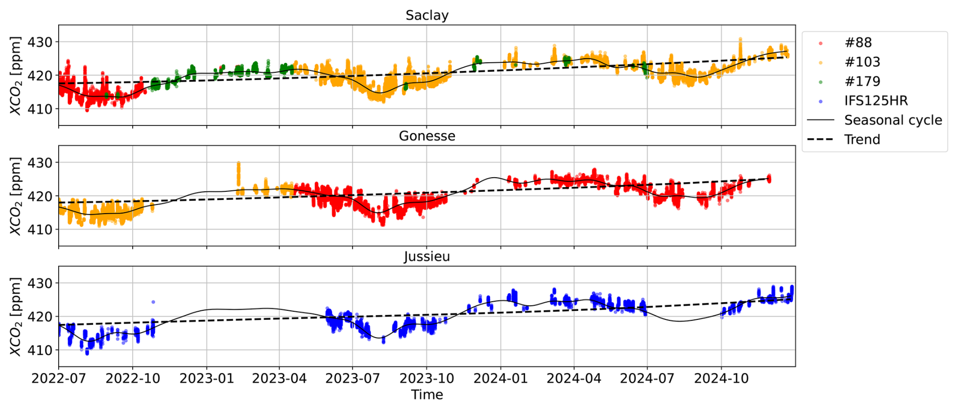
Figure 6 Time series of XCO₂ measurements in Saclay, Gonesse and Jussieu, from 1 July 2022 to 31 December 2024. The black continuous lines show the combination of the seasonal cycle and the growth rate. The black dotted lines show the rising trend of XCO₂.

At synoptic scale, variations occur on spatial scales much larger than the inter-station distances considered here. Therefore, the three sites show consistent seasonal cycles and linear growth rates. Compared with surface in-situ records (∼ 20 ppm amplitude in Paris), the column amplitude is much smaller due to vertical mixing. It is important to note that seasonal and long-term signals are very similar at the regional scale (Doc et al., 2024), and therefore cancel each other out when calculating inter-station gradients, so that they do not affect plume detection.

4.2 Short term variations and case study

EM27/SUN instruments acquire spectra at 1 min resolution. At such scales, most variability is noise (see Sect. 3.2), and smoothing over 20 min is appropriate. Nonetheless, large short-term variations occasionally occur, over a period of a few hours. Due to their amplitude, typical duration of variation, and correspondence with wind directions connecting the measuring stations, these appear to be most likely geophysical (urban plumes).

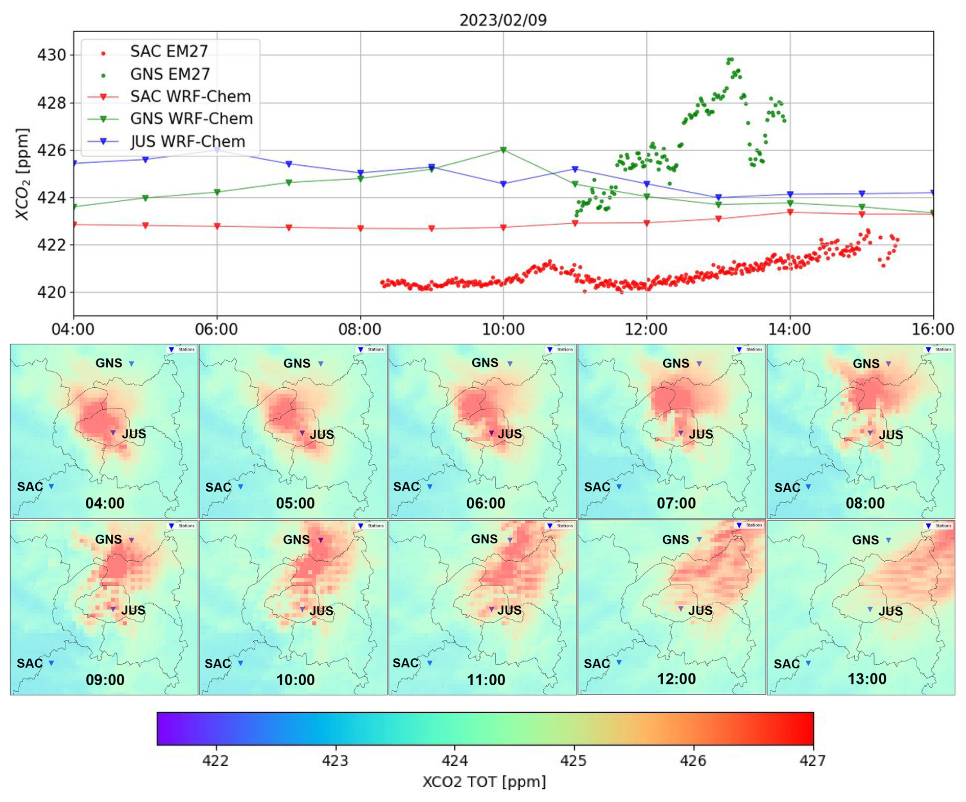
Figure 7 Time series of measured (dots) and WRF-Chem simulated (triangles) XCO₂ in SAC, GNS and JUS on 9 February 2023 (upper panel). Maps of XCO₂ from WRF-Chem simulation on 9 February 2023 between 04:00 and 13:00. (lower panels).

A notable event occurred on 9 February 2023, when XCO₂ at Gonesse increased by ∼ 6 ppm in 2 h. Figure 7 shows the measured and WRF-Chem simulated (see Sect. 5.2.1–5.2.2) XCO₂ time series at Saclay, Gonesse, and Jussieu. Between 11:00 and 13:00, XCO₂ at Gonesse rose from 423 to 429 ppm, then dropped by 4 ppm within 30 min, followed by a 2 ppm rebound. At Saclay, only a modest increase (∼ 1 ppm) was observed during that period.

WRF-Chem simulations reproduce some features: at Gonesse, a rise of ∼ 2 ppm is simulated between 04:00 and 10:00, followed by stabilization; Saclay shows no enhancement. Simulated maxima are lower and shifted in time compared with the observations, suggesting model limitations.

The lower panels of Fig. 7 show simulated CO₂ maps between 04:00 and 13:00. They reveal nighttime accumulation over Paris under calm conditions, followed by north-north-eastward transport. At 10:00, Gonesse lies in the plume core (426 ppm), while Saclay remains in background air. As winds shift, the plume moves westward, explaining the rapid decrease observed at Gonesse.

This episode, remarkable for its amplitude, is consistent with a CO₂ plume from Paris. However, the discrepancy in amplitude (7 ppm observed vs. 3 ppm simulated) and timing highlights the difficulty of comparing measurements with models near large sources. Errors in transport fields can dominate apparent source mismatches. Therefore, caution is required when interpreting model–measurement differences solely as inventory biases (Bréon et al., 2015).

5 Analysis of spatial XCO₂ gradients

Because there is significant uncertainty in the background (upwind) CO₂ concentration, we use spatial gradients (denoted Δ) between stations to estimate emissions. In this section, we analyse gradients with the WRF-Chem model (Lian et al., 2023) to separate their components and to interpret the observed signals. The configuration used here simulates CO₂ only, so – even though CH₄ and CO are relevant urban tracers – this section focuses solely on CO₂.

Atmospheric CO₂ concentrations are shaped by transport and by surface exchanges (sources and sinks), namely:

• Anthropogenic emissions resulting from the combustion of fossil fuels (road traffic, residential heating, industry, etc.);

• Biogenic fluxes, which can be either negative or positive depending on the balance between photosynthesis and respiration.

Gradients between total columns (measured and/or simulated) at two distinct geographical points carry information about these fluxes. In an Eulerian framework, when the wind direction aligns with the inter-station axis, both sites sample the same air mass after it has crossed the urban area. In a Lagrangian view, the parcel travels from the upwind to the downwind site and the difference integrates the fluxes encountered between the two locations. Under such conditions, the gradient can be assimilated in an inverse-modelling framework.

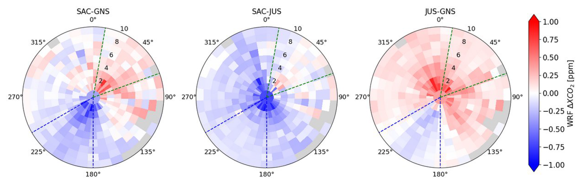
Figure 8 Simulated XCO₂ differences between pairs of stations as a function of wind speed (radius) and wind direction (angle). Green and blue marks indicate wind sectors representative of flow from Paris toward Saclay and toward Gonesse, respectively (see Fig. 1).

Figure 8 displays WRF-Chem simulated gradients between pairs of stations for all hours between 09:00 and 16:00 local time, over July 2022–December 2024. The wind-sector selections (green and blue) reflect situations when the Paris plume is expected to be transported toward Saclay or Gonesse. In what follows, we compare measured gradients with those simulated by WRF-Chem in order to assess how column measurements can constrain emissions.

The simulated gradients are mostly within the range of −0.5 to 0.5 ppm. They exhibit a strong dependence on wind direction, with clear sign reversals that reflect the transport of the CO₂ plume emitted from Paris and its surrounding urban area. The wind sectors defined geometrically (see Sect. 2.1) align well with the simulated plume patterns. A significant dependence of the gradient on wind speed is also observed. Under low wind speed conditions (1 to 3 m s⁻¹), the CO₂ plume disperses slowly, leading to greater local accumulation and resulting in gradients exceeding 1 ppm. Conversely, under stronger winds (8 to 10 m s⁻¹), the plume is more efficiently transported and diluted within a larger air mass, yielding much smaller gradients, typically between 0 and 0.25 ppm. These results clearly highlight the average signal associated with the Paris plume. This is precisely the signal that the measurements aim to capture and characterize.

In the following, we compare the measured gradients with those simulated by WRF-Chem, in order to assess the potential contribution of column measurements to the optimization of the statistical emission inventory used in the model. A previous study (Lian et al., 2023) using in-situ surface measurements from the Paris network over a six-year period indicates that the inventory is underestimated by between 2 % and 20 %, depending on the month (minimum in winter and maximum in late spring/summer). There is a significant uncertainty in this estimate, however, due to the poor representation of vertical mixing in the model. Column measurement sensitivity to vertical mixing is much smaller, which is then an advantage when comparing measured and modelled concentration with the objective of assessing the emissions.

5.1 Measured XCO₂ gradients

As indicated in Sect. 1, we use hourly averages of wind speed and direction measured at Saclay (100 m above ground level in an open area) as representative of the regional wind conditions. EM27/SUN instruments acquire one spectrum per minute, which we then aggregate into hourly averages (to correspond to the time step of simulated data). We used the measured gradients calculated between the different pairs of stations (SAC-GNS, SAC-JUS and JUS-GNS), and compare them to the simulated gradients in Sect. 5.2.

Figure 10 (top panels) shows measured gradients as a function of wind speed (radius) and upwind wind direction (angle) for the three station pairs.

For SAC–GNS (left-hand panel), the gradient depends strongly on wind direction: south-westerlies generally yield negative values (plume toward Gonesse), while north-easterlies yield positive values (plume toward Saclay). Typical magnitudes are around +1 ppm when flow is aligned with the SW–NE axis. These are of the same order of magnitude as those observed during the preliminary campaign in 2015 (Vogel et al., 2019) or what can be observed in other large urban areas with population characteristics similar to Paris (Berlin, Hase et al., 2015; Zhao et al., 2019, Munich, Dietrich et al., 2021; Zhao et al., 2023 or Mexico, Che et al., 2024). On the other hand, we would theoretically expect a sharp dependency on wind speed, which is not clearly observed here in measured and simulated gradients.

The Jussieu station is located in the city center, and measurements there exhibit higher noise than at Saclay and Gonesse (see Sect. 3.2), which complicates the detection of small gradients. For SAC-JUS (middle panel), when wind speed < 3 m s⁻¹ the gradient is systematically negative (down to −1.5 ppm), regardless of wind direction. This reflects CO₂ accumulation above central Paris (Jussieu) relative to suburban Saclay. For wind speed > 3 m s⁻¹ and NE winds, the gradient becomes positive (up to +0.75 ppm), consistent with plume transport toward Saclay. The amplitude is roughly half that of SAC-GNS under comparable conditions. For south-westerlies, the SAC-JUS gradient varies between −1 and +1 ppm with no clear pattern, suggesting a weaker, locally variable column signal for this pair.

For JUS-GNS (right-hand panel), the behaviour is similar. At low wind (<2–3 m s⁻¹), gradients are mostly positive (∼ +1 ppm), consistent with a stronger urban load over Jussieu than over Gonesse. At higher wind speeds, south-westerlies yield negative gradients (down to −1.5 ppm), indicating plume export toward Gonesse; north-easterlies show more variable behaviour. Under NE winds, positive gradients tend to be slightly stronger than the SAC-JUS case under SW winds, consistent with Gonesse being more urbanized than Saclay, with higher emissions.

5.2 Comparison between measured and simulated XCO₂ gradients

5.2.1 WRF-Chem framework

We use WRF-Chem (Weather Research and Forecasting model coupled with Chemistry) to compare observed and simulated gradients. Following Lian et al. (2023), three nested domains at increasing spatial resolution are employed:

• D01: about 1500 × 1500 km, fully covering France, at 25 km resolution;

• D02: about 550 × 500 km, covering most of northern France, at 5 km resolution;

• D03: about 150 × 150 km, centered on Paris, at 1 km resolution.

In each case, the temporal resolution of the outputs is one hour. A CO₂ dynamical emission inventory (Lian et al., 2022, 2023) is used to model the anthropogenic emissions. It has been developed by origins.earth, on the base of activity data such as traffic count and gas use. The Vegetation Photosynthesis and Respiration Model (VPRM) (Mahadevan et al., 2008) is used to simulate biogenic fluxes. This model used a detailed description of the vegetation cover and use meteorological data (temperature, solar irradiation, precipitation, etc) to constrain the vegetation photosynthetic activity and respiration. Global atmospheric simulations from CAMS (Tang et al., 2018) are used as boundary conditions for the D01 domain. The D01 and D02 domain simulation provide the boundary conditions for the simulations of the D02 and D03 domains.

The model uses 42 vertical levels, between the surface and an atmospheric level around 100 hPa (∼ 15 km). CO₂ concentrations above the 100 hPa level have negligible spatial variability so that we use the CAMS simulation forecast to complete the profiles to top of the atmosphere. Note that the atmospheric transport from the surface to the stratosphere takes at least several days (except for very specific atmospheric conditions) so that the contributions of the biogenic and anthropogenic fluxes within our study domain to that atmospheric concentration can be assumed to be zero above 100 hPa.

5.2.2 WRF-Chem CO₂ data extraction and columns computation

For our analysis, we use the results of the simulations with the higher resolution domain (D03) (see Sect. 5.2.1). The WRF-Chem outputs, together with the CAMS profiles above 100 hPa, are used to describe the full vertical profile at the location of the remote sensing stations. We then use Eq. (4) to calculate the column, to account for the vertical sensitivity of the EM27 and TCCON measurements. Note that the vertical sensitivity depends on the solar zenith angle, so that we do use this parameter as input to derive the modelled column concentration. We compute the total column concentration, but also the biogenic and anthropogenic contributions from the simulation domains as these are transported independently by the WRF model.

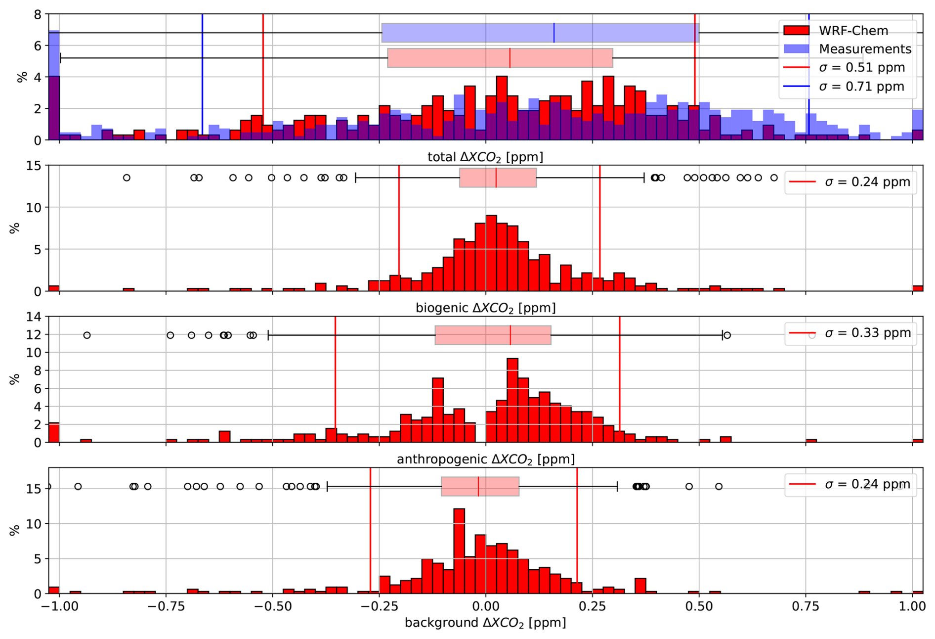
Figure 9 Histogram of total (first panel), biogenic (second panel), anthropogenic (third panel) and background (fourth panel) measured (total ΔXCO₂ only) and WRF-Chem simulated ΔXCO₂ Saclay-Gonesse spatial gradients, from 1 July 2022 to 31 December 2024. For each panel, the boxplots of the distributions (first and third quartiles) are given together with the standard deviations of the distribution (vertical lines). The frequencies outside of the figure range are indicated with a single bin at the extremes of the range.

Figure 9 shows histograms of the simulated (red) and measured (blue) column-averaged CO₂ gradients (ΔXCO₂) between Saclay and Gonesse (SAC-GNS), computed by WRF-Chem from 1 July 2022 to 31 December 2024. The model has been sampled at times when an observation is available.

The upper panel shows the distribution of total gradients simulated by WRF-Chem. The distribution is broad with no well-marked mode in the distribution. There is however, a slight predominance of positive values, with a median gradient of 0.06 ppm and 50 % of the values ranging between −0.23 and 0.30 ppm. Only 5 % of the simulated gradients fall outside the interval [−1, 1] ppm, with extreme values of −2.52 and 1.78 ppm.

The upper panel also displays the distribution of measured gradients (in blue), which is likewise not centered on a clearly defined value. The distribution shows a majority of positive values, with a median of 0.16 ppm and 50 % of the gradients between −0.24 and 0.50 ppm. This distribution is therefore broader than that of the simulated gradients. This is confirmed by the higher proportion of values outside the interval [−1, 1] ppm (9 %) and by more extreme values of −5.94 and 2.07 ppm. The distributions of simulated and measured gradients are fairly consistent. Note that, based on the statistics on the prevailing winds (see Fig. 1) from the South West, one would expect a predominance of negative values, which is not found in Fig. 9 results. This discrepancy may result from the clear sky requirements for XCO₂ gradients measurements, when a clear sky is more likely in North-East wind condition rather than when the wind blows from the South-West. Indeed, for the cases used in Fig. 9, the proportion of cases in the SW/NE wind sectors defined in Fig. 1 is $\mathrm{60}\mathit{\%}/\mathrm{40}$ %, which is much more balanced than the overall statistics.

The biogenic component (second panel of Fig. 9) shows a distribution close to a Gaussian centered around 0 (median: 0.02 ppm), with 50 % of the values between −0.07 and 0.12 ppm. The near symmetry of the distribution indicates that CO₂ uptake by the biogenic sink does not generate a major imbalance in the gradients simulated by WRF-Chem, as it tends to compensate at the spatial scale considered. This component is therefore relatively stable and largely constrained by external drivers such as solar radiation and vegetation phenological cycles.

The third panel presents the distribution of the anthropogenic component of the gradients simulated by WRF-Chem. A clear bimodal distribution is observed, centered around two distinct values: approximately −0.15 and 0.10 ppm. These two modes correspond to the two wind sectors that have been selected in this analysis and to the transport of urban emissions from Paris toward Saclay and Gonesse. A predominance of positive values is observed, which is counter-intuitive but consistent with the findings for total gradients in the upper panel. At the first order, one expect that the gradient linked to anthropogenic emissions are positive for the case identified in the North-East sector, and negative for the South-West sector. Although it is mostly so, we have identified a significant fraction of cases when the sign of the anthropogenic gradient is not as expected. This is because we use the mean wind speed at the exact time of the observation, while the spatial structure of the concentration signal depends on the history of the atmospheric transport. They are therefore cases when the sign of the gradient is not as expected based on the wind speed information.

The background ΔXCO₂ contribution (fourth panel of Fig. 9) is characterized by a symmetrical distribution, centered on 0 ppm (median value: −0.01 ppm). The background concentration should be very similar in the whole domain at any given moment. Thus, a narrower distribution of background gradients between SAC and GNS could be expected. We observe only 50 % of simulated background gradients between −0.10 and 0.08 ppm. Nevertheless, almost 90 % are between −0.2 and 0.2 ppm which confirms that the background varies across the domain, with a low but non-neglectable amplitude. However, occasional episodes with larger differences between the background at the two stations do occur and must be taken into account when interpreting the total gradient in relation to urban emissions.

This figure also allows us to assess the relative importance of each component's contribution to the overall gradient. With a standard deviation of 0.28 ppm and an interquartile range of approximately 0.25 ppm, the anthropogenic contribution appears to play a dominant role as a driver of the total gradient's variability. Nevertheless, the biogenic and background components exhibit standard deviations of 0.14 and 0.19 ppm, and interquartile ranges of approximately 0.10 and 0.15 ppm, respectively. These values indicate that, although their influence is lower than that of the anthropogenic signal, their contribution to the total gradient remain non-negligible.

The relative contributions of the different components to the total gradient are further illustrated by their correlations (see Fig. S6). Significant correlations are found between each component and the total gradient ($r_{\mathrm{bio};\mathrm{tot}}=\mathrm{0.70}$, $r_{\mathrm{ant};\mathrm{tot}}=\mathrm{0.66}$ and $r_{\mathrm{bck};\mathrm{tot}}=\mathrm{0.51}$), confirming the dominant roles of the anthropogenic and biogenic gradients (particularly in spring), as well as the non-negligible contribution of the background to the total gradient. In contrast, the very weak correlations among the components themselves ($r_{\mathrm{ant};\mathrm{bio}}=\mathrm{0.22}$, $r_{\mathrm{bck};\mathrm{ant}}=\mathrm{0.07}$ and $r_{\mathrm{bio};\mathrm{bck}}=-\mathrm{0.05}$) indicate that they are largely independent from one another.

Overall, the biogenic and background contributions are centred on zero, and relatively small with respect to the inconsistency between the simulated and observed distributions of the gradients (top panel of Fig. 9). It is then unlikely that these contributions have a much larger amplitude and can then explain this discrepancy. At present, we have no explanation for the observation-modeled differences.

5.2.3 Correlations between measured and simulated XCO₂ gradients

The simulated gradients are modulated by biogenic (VPRM) and anthropogenic (Origins.earth) fluxes between the two stations, with strong seasonal and synoptic variability. Comparing measured and simulated gradients helps identify which component and/or which modelling aspect most likely drives the discrepancies.

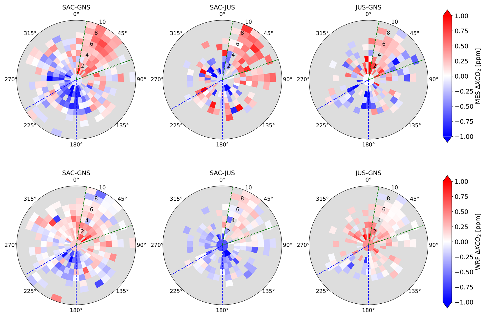
Figure 10 Measured (top) and simulated (bottom) XCO₂ gradients between pairs of stations as a function of the wind speed (radius) and wind direction (angle), from 1 July 2022 to 31 December 2024. The green and blue lines indicate the range of wind directions considered to be representative of airmasses coming from Paris to Saclay and Gonesse respectively (see Fig. 1).

The simulated and measured gradients between pairs of stations are shown in Fig. 10. The data have been acquired between 1 July 2022 and 31 December 2024 and the simulated data are for the same days and time when measurements are available. The range of the simulated data is [−1; 1] ppm, which is similar to the range of the measured gradients. For the Saclay-Gonesse (SAC-GNS) gradient, there is some consistency between the measured and modelled gradients, which are mostly negative (i.e. XCO_{2_SAC} < XCO_{2_GNS}) for south-westerly winds and positive (i.e. XCO_{2_SAC} > XCO_{2_GNS}) for north-easterly winds. For the Saclay-Jussieu (SAC-JUS) gradient, the simulated gradients are predominantly negative in all wind conditions, which can be understood as the impact of local emissions in the vicinity of the Jussieu station, at the center of Paris. However, this is not in agreement with the measurements that show mostly positive gradients whenever the wind speed is greater than 3 m s⁻¹. There is no obvious explanation for this inconsistency. For the Jussieu-Gonesse (JUS-GNS) gradient, there is a better consistency between the measured and modelled patterns, although far from perfect. The gradients are mostly positive, in both the model and the measurements.

For the three pairs of stations, the complete set of simulated gradients over the entire study period reveals the expected and characteristic signature of the plume originating from an urban area such as Paris (see Fig. 8). However, a direct comparison between simulated and observed gradients can only be performed at the timestamps for which measurements are available. Consequently, the number of data points included in Fig. 10 is considerably smaller than the full set of simulated gradients. As a result, the average Paris plume appears much less distinct and is substantially noisier.

In the following, we analyse the concentration gradients whenever the wind direction is within the sectors identified in Fig. 1, for which the gradient is the most affected by the Paris emissions. A first order correction of the emissions described by the inventory is related to the slope of the best linear fit between measured and modelled gradient. We quantify the ability of the model to reproduce the observed gradients by the Pearson correlation coefficient between measured and modelled gradients.

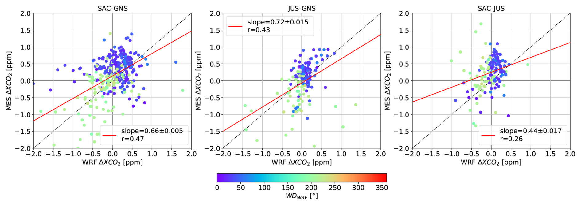
Figure 11 Scatter plot of the modelled (x-axis) and measured (y-axis) XCO₂ gradients between pairs of stations, from 1 July 2022 to 31 December 2024. The colour of the data points indicate the wind direction. The red line is the result of the best linear fit. Statistical parameters (slope of the fit, correlation) are provided.

Figure 11 shows a scatter plot of the modelled and measured gradients. Each graph is for a pair of stations (SAC-GNS, JUS-GNS and SAC-JUS on the left, middle and right panels of the figure respectively). Linear fits are represented by red solid lines. Note that the measured and modelled wind direction may differ. Data points for which the direction differs by more than 50° have been removed.

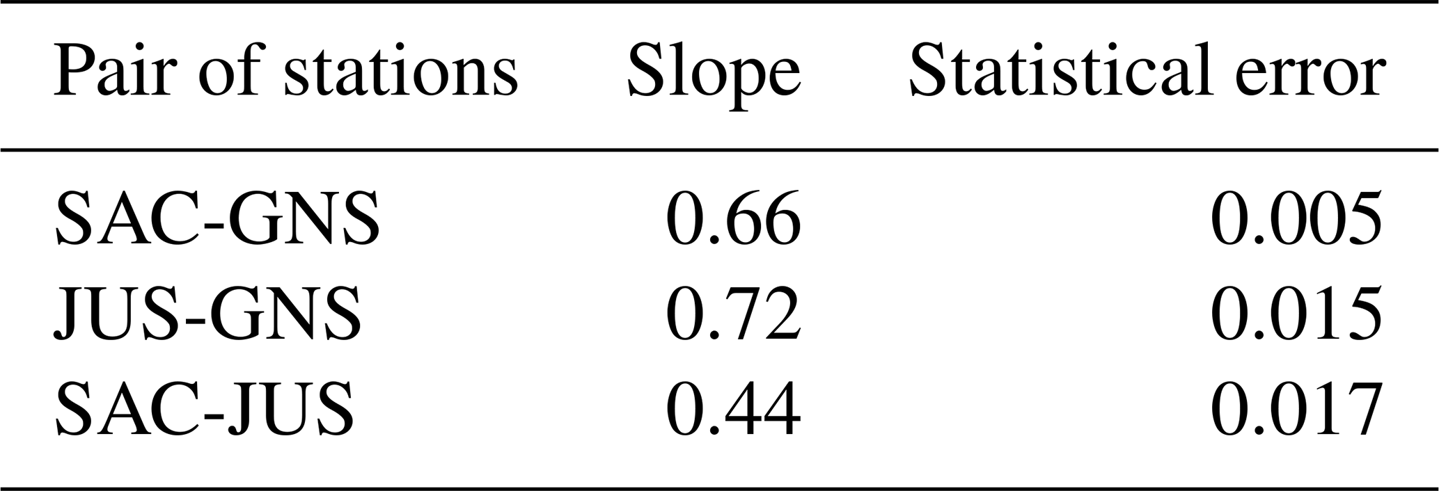
Of the three pairs of stations, the best correlation is found between Saclay and Gonesse (r_SAC-GNS=0.47), the two stations on either side of the urbanised area of Paris. Such moderate correlation indicates significant discrepancy between measured and modelled concentration, it is similar to that found with similar analysis over other cities (c.f. Sect. 1). The slope of 0.66 indicates an over-estimation of the emissions in the a priori inventory. A better agreement between measured and modelled gradients (but not a better correlation) could be obtained through a strong reduction of the a priori emissions. However, the amplitude of the necessary reduction (34 %) is not realistic as the uncertainty on the emission inventory is much lower, and has been evaluated against surface concentration measurements (Lian et al., 2023). The analysis of the gradients from the other pairs of stations is complicated by the noise of the JUS instrument that is significantly larger than those as SAC and GNS, and significant with respect to the signal that is being analysed (see Sect. 3.2). The additional noise is an explanation for the even lower correlation for the JUS-GNS (0.43) and SAC-JUS (0.26) pairs of stations. The best fit slope is also lower than 1 (0.72 for JUS-GNS and 0.44 for SAC-JUS). The best linear fit indicates a statistical error that are relatively small (0.005 for SAC-GNS, 0.015 for JUS-GNS, and 0.017 for SAC-JUS), so that a slope significantly smaller than 1 is a result that is statistically robust. These results are summarized in Table 4. However, given the very low correlation between measured and modelled gradient, and the case study analysis of Fig. 7, it is clear that the atmospheric transport modelling is far from perfect, so that there is little value in the result of the liner fit analysis.

Table 4 Slopes and statistical errors of linear fits of measured vs simulated XCO₂ gradients between pairs of stations presented in Fig. 11.

The correlations between simulated and measured gradients vary throughout the year. Summer (June, July, August) shows the lowest correlation (r_SAC-GNS=0.28 and s_SAC-GNS=0.34), likely due to the dominance of the biogenic signals which are more difficult to simulate precisely and a reduction in anthropogenic emissions during this period. In contrast, autumn shows the highest correlation (r_SAC-GNS=0.70 and s_SAC-GNS=0.94), when biogenic activity is minimal and anthropogenic sources dominate. For similar reasons, one might expect even stronger correlations in winter, but there are few valid data during that season to verify this hypothesis.

In order to determine the origin of the weak correlations between the WRF-Chem simulated and measured gradients, we could use the same model with a different a priori inventory and/or another model with the same a priori inventory. As these data are not yet available, this work will be explored in a later study. We can nevertheless use the columns calculated from the outputs of other models to see whether the behaviour observed with WRF-Chem is similar. We use the high-resolution (9 km) forecasts from CAMS (Tang et al., 2018) to calculate the columns and gradients between pairs of stations, using the same methodology as for WRF-Chem outputs.

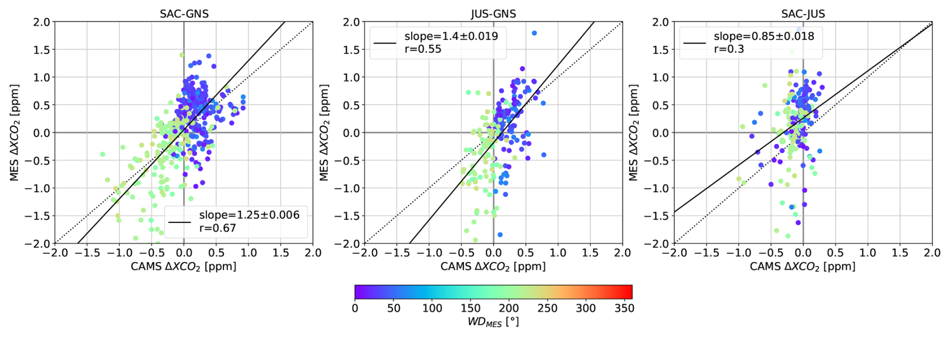
Figure 12 Same as Fig. 10 but using the CAMS global scale high-resolution (9 km) forecasts rather than the WRF-Chem simulation.

Figure 12 shows the scatter plot of the modelled and measured concentration gradients for the three pairs of stations but using the CAMS global scale forecasts with a resolution of 9 km (Tang et al., 2018). Between the Saclay and Gonesse stations, the Pearson coefficient is relatively high (0.67), revealing good agreement between the gradients measured and simulated by CAMS. As with WRF-Chem, it is the pair of stations that shows the best match between simulations and measurements. The slope of 1.25 shows a 25 % underestimation of the modelled gradients which could be representative of an underestimation of emissions in the a priori emissions inventory used by CAMS (CAMS-GLOB-ANT described in Soulie et al., 2024). The use of gradients involving the central Paris station (JUS-GNS and SAC-JUS) is better than with WRF-Chem but remains worse than the SAC-GNS pair. Indeed, we observe weaker correlations (0.55 and 0.30 respectively) than for the SAC-GNS pair (0.67). The statistical error associated with the SAC-GNS gradients (0.006) is very close to the one obtained using WRF-Chem simulations under the same configuration. This very small difference suggests that both slope estimated are statistically robust, and that observed differences are not driven by random error, but more likely by discrepancies in the atmospheric transport simulations or emissions. For the JUS-GNS and SAC-JUS gradients, the statistical errors remain low but are noticeably higher than that of SAC-GNS (0.019 and 0.018, respectively), indicating the presence of some random uncertainty, although it is not dominant. This higher error could be due to measurement noise from the high-resolution spectrometer at Jussieu (see Sect. 3.2). In the same way as with WRF-Chem, the lowest correlation is observed between SAC and JUS (only 0.30). The underestimation of the emissions inventory (25 %) seems more reasonable than the overestimation that seems to appear for WRF-Chem (34 %). This confirms that further research is needed on WRF-Chem outputs together with column measurements.

6 Conclusion and outlook

We have presented two years of total column measurements of CO₂, CH₄, and CO in the Paris metropolitan area, based on a network of three FTIR spectrometers (Saclay, Gonesse, and Jussieu). Together with long-standing in-situ observations, this network provides a unique framework to investigate the urban carbon cycle at regional scale.

Instrumental characterization shows that EM27/SUN spectrometers deliver robust and precise retrievals, with uncertainties of ∼ 0.2 ppm for XCO₂, 1.2 ppb for XCH₄, and 2 ppb for XCO for EM27/SUN measurements and ∼ 0.7 ppm for XCO₂, 3.5 ppb for XCH₄, and 4.1 ppb for XCO for IFS 125 HR measurements. The higher resolution instrument shows higher noise levels than the EM27/SUN, due to spectroscopic effect (Galli et al., 2014; Langerock et al., 2025). Side-by-side comparisons demonstrate excellent network consistency, while sensitivity analyses confirm that biases linked to solar zenith angle, a priori profiles, or pressure errors remain modest. These results establish confidence in the use of total column gradients across the Paris region.

A significant sensitivity to the solar zenith angle is also highlighted, with a systematic error significantly greater than 0.1 ppm for SZA above 60°. Excluding observations with SZA greater than this threshold would preclude most observations during the winter season, which is strongly undesirable given the small number of measurements taken at this time of year. There is therefore a need to understand and correct the SZA-related bias at large angles.

Geophysical analyses highlight seasonal and synoptic variability, with gradients of 0.5–1.5 ppm typically observed between upwind and downwind stations when the wind aligns with the network axis. Case studies demonstrate the capacity of the network to capture sharp plume events, although their amplitude and timing are not always well reproduced by simulations. Biogenic contributions are shown to be smaller but not negligible, especially in spring.

Comparisons between measured and simulated gradients using WRF-Chem suggest that emissions reported by the AirParif inventory (and used as a priori in the model) are overestimated by approximately 34 % over the whole study period. However, the correlation between measured and modelled gradients is poor, most likely due to uncertainties in the atmospheric transport modelling. The large spread between the measured and modelled concentration cast doubt on the reliability of the result based on a best linear fit. In addition, the finding of a strong overestimate in the inventory contrasts significantly with the results of a similar study based on in-situ surface CO₂ concentration measurements. That study, published in Lian et al. (2023), concluded that emissions were underestimated by 2 % to 20 %, depending on the month with a maximum in late spring/summer and a minimum in winter. When averaged over the full atmospheric column, the anthropogenic signal is not strong enough when accounting for measurement noise, biogenic variability and model uncertainty. The approach using surface measurements Lian et al. (2023) involves a degree of uncertainty due to the modelling of vertical atmospheric transport. This is not (or only slightly) the case for total column measurements. For this reason, total column measurements provided an interesting perspective in the optimisation of emissions inventories.

During spring and summer, when the weather is often favourable for the FTIR XCO₂ observations, the anthropogenic signal is small (no heating-related emissions) and the poorly constrained biogenic contribution is significant. Conversely, in the fall and winter, the anthropogenic signal dominates the XCO₂ gradient, but few valid observations are available due to the weather.

This explains why, under current conditions, total column CO₂ measurements in the Paris urban area do not provide a robust constraint on the emission inventory.

Overall, the Paris FTIR network provides clear evidence that total column observations can detect and quantify urban CO₂ plumes. However, robust emission estimates require further improvements in transport modelling, as well as longer time series to better disentangle anthropogenic and biogenic contributions across seasons.

Looking ahead, several developments could enhance the role of total column networks in urban carbon monitoring:

• Integration with satellites: Column measurements provide a natural bridge to satellite missions such as MicroCarb (launched in July 2025) and the forthcoming CO₂M. Combined ground-satellite analyses will strengthen emission estimates and help validate space-based products.

• Network expansion: Adding stations along other wind axes would improve coverage of plume variability and facilitate inverse modelling.

• Model improvements: Higher-resolution meteorology, improved boundary layer schemes, and ensemble transport simulations would reduce uncertainties in model-data comparisons.

• Multi-species approaches: Joint use of CH₄ and CO columns with CO₂ may help separate emission sectors and provide cross-validation with independent tracers.

The Paris experiment illustrates both the promise and the challenges of using total column observations for urban greenhouse-gas monitoring. Continued efforts to integrate ground-based, airborne, and satellite observations with advanced modelling will be key to establishing reliable, policy-relevant emission estimates for cities worldwide.