the Creative Commons Attribution 4.0 License.
the Creative Commons Attribution 4.0 License.
 | 24 Jun 2026
Reassessment of the glyoxal-to-formaldehyde ratio RGF as a proxy for VOC source identification
Simon Bittner
Andreas Richter
Bianca Zilker
Sebastian Donner
Thomas Wagner
Alexandros Panagiotis Poulidis
Leonardo Alvarado
Mihalis Vrekoussis
The glyoxal-to-formaldehyde ratio (RGF) has been proposed as a proxy to distinguish sources of volatile organic compounds (VOCs) in the atmosphere. However, the interpretation of its variability remains uncertain because of the diverse processes that affect VOC emissions and chemistry. In this study, we revisit the applicability and limitations of RGF using multi-year ground-based MAX-DOAS measurements at four distinct sites: two biogenic (Orléans, France, and ATTO Tower, Brazil) and two anthropogenic (Athens, Greece, and Incheon, South Korea).
The results show higher RGF in anthropogenic environments and lower at biogenic sites. Seasonal RGF patterns are broadly consistent across sites, with lower values in summer and higher values in winter, driven by formaldehyde variability. Diurnal cycles are primarily controlled by glyoxal variability and are more pronounced at urban sites, which also show a weekend reduction of 10 %. Correlations between RGF and NO2 vary, even among anthropogenic stations, highlighting the importance of local emission contributions. Increasing temperatures from 15 to 35 °C decrease RGF by up to 1.9 percentage points across all sites, driven by the stronger temperature response of formaldehyde compared to glyoxal. We further discuss four effects that complicate cross-study comparability of RGF: differences in measurement volume, vertical sensitivity, temporal sampling, and the impact of averaging-ratioing order.
Our findings suggest that ground-based remote sensing RGF contains valuable diagnostic information about VOC source environments. However, its use as a universal proxy remains challenging, as our incomplete understanding of the various effects currently limits the reliable use of RGF for VOC source attribution.
- Article
(4498 KB) - Full-text XML
-
Supplement
(1743 KB) - BibTeX
- EndNote


The European Environmental Agency reported in 2024 that meeting World Health Organization (WHO) air quality standards across EU Member States could prevent 239 000 annual deaths from fine particulate matter (PM2.5), 70 000 from tropospheric ozone (O3), and 48 000 from nitrogen dioxide (NO2) exposure (European Environment Agency, 2024). Globally, the situation is comparable, with particularly high numbers of premature deaths occurring in Asia (Lelieveld et al., 2015).
Tropospheric O3, which has strongly enhanced concentrations in summer smog, is associated with increased cardiovascular and respiratory mortality (Bell et al., 2004; Turner et al., 2016). Its formation requires two precursors in the presence of sunlight: nitrogen oxides () and volatile organic compounds (VOCs) (Haagen-Smit, 1952). Understanding the role of these individual components is essential for effective ozone mitigation strategies. NOx emissions originate primarily from fossil fuel combustion, followed by natural sources such as biomass burning, soil emissions, and lightning (Ehhalt et al., 2001; Seinfeld and Pandis, 2006).
Investigating the origin of VOCs, focussing on non-methane VOCs, is more challenging, as they encompass a large and diverse group of compounds. In addition to their role in tropospheric ozone formation, they contribute to the formation of secondary organic aerosols (SOA) (Hallquist et al., 2009; Derwent et al., 2010) and cloud condensation nuclei (Zheng et al., 2020; Liu and Matsui, 2022). Their sources are generally categorised as biogenic, pyrogenic, or anthropogenic (Vrekoussis et al., 2010).
Among these categories, biogenic VOC emissions represent the largest share of total VOC emissions (Guenther et al., 1995; Stavrakou et al., 2009b). Vegetation emits up to 10 000 different VOCs (Goldstein and Galbally, 2007), which are involved in a wide range of processes, including growth, development, communication, and defence against herbivores. Isoprene (C5H8) is the most commonly emitted VOC species, followed by monoterpenes (C10H16). Emission rates are influenced by many factors and vary across plant species, plant parts, and even leaf age (Laothawornkitkul et al., 2009; Zhang et al., 2023). Another significant share of VOC emissions originates from pyrogenic sources, such as biomass burning. The combustion of biogenic material releases a complex mixture of species into the atmosphere, including a wide variety of VOCs. The composition of these emissions strongly depends on the material being burned (Gilman et al., 2015) and on moisture content (Paris et al., 2022). Anthropogenic VOCs are emitted by a variety of sources. The Community Emissions Data System (CEDS) inventory indicates that energy production, road transportation, residential activities, and solvent usage are the dominant processes/sectors on a global scale (McDuffie et al., 2020).
Among VOC species, glyoxal (CHOCHO) and formaldehyde (HCHO) are key intermediate products of VOC oxidation in the atmosphere (Fu et al., 2008; Chan Miller et al., 2016). HCHO is the most abundant atmospheric aldehyde, with primary emissions from vehicle exhausts (Nelson et al., 2008) and biomass burning (Lee et al., 1998; Andreae and Merlet, 2001). Its main source, however, is formation through secondary production from VOC oxidation (Fortems-Cheiney et al., 2012) and methane (CH4) oxidation, which determines its background levels (Franco et al., 2016). HCHO is removed from the atmosphere by photolysis, reaction with hydroxyl radicals (OH), and deposition (Stavrakou et al., 2009b). Its typical tropospheric lifetime around midday is about 3 h (Dienhart et al., 2021).
Glyoxal, the smallest dicarbonyl compound, shares similar sources with HCHO: primary emissions from biomass burning (Zarzana et al., 2017, 2018) and biofuel use (Fu et al., 2008), as well as secondary formation via VOC oxidation. Primary glyoxal emissions are generally small compared to its secondary production (Stavrakou et al., 2009a; Silva et al., 2018). Its tropospheric lifetime is short, on the order of a few hours (Volkamer et al., 2007; Myriokefalitakis et al., 2008; Fu et al., 2008). Glyoxal is removed through photolysis, reactions with OH, and both dry and wet deposition (Myriokefalitakis et al., 2008), with an additional important sink via SOA formation (Stavrakou et al., 2009a).
The ratio of glyoxal-to-formaldehyde (RGF) was proposed by Wittrock et al. (2006) and Vrekoussis et al. (2010) as a potential proxy for differentiating VOC source types. Because CHOCHO and HCHO have similar sources and loss processes, subtle differences in VOC mixtures or source-specific yields are expected to be reflected in RGF. The interpretation of RGF as a diagnostic for VOC sources has remained inconsistent since its introduction. Vrekoussis et al. (2010) analysed 2 years of GOME-2 satellite data and found a strong spatial correlation between RGF and VOC source categories, proposing a threshold of 4 % to distinguish anthropogenic sources (below) from biogenic or pyrogenic origins (above). They further observed decreasing RGF with higher NO2 levels and increasing values with greater vegetation density, quantified by the Enhanced Vegetation Index (EVI).
Subsequent studies, however, produced mixed and sometimes contradictory results (Irie et al., 2011; DiGangi et al., 2012; MacDonald et al., 2012; Li et al., 2014; Chan Miller et al., 2014). Based on airborne in-situ data, Kaiser et al. (2015) shifted the focus toward VOC precursor speciation, finding that monoterpenes yield high RGF values while isoprene yields low values. DiGangi et al. (2012) went further, proposing an interpretation opposite to that of Vrekoussis et al. (2010), with lower RGF associated with biogenic sources and higher values with anthropogenic or pyrogenic origins. More recently, Chen et al. (2023) reported a positive correlation of RGF with both EVI and NO2 using TROPOMI data, and proposed that anthropogenic VOC emissions can be identified where RGF > 4 % with additional constraints on EVI and HCHO columns. Hong et al. (2024) further argued that primary HCHO emissions bias RGF, and proposed the ratio of CHOCHO to secondary HCHO as a more reliable metric.
Further complexity was added by MAX-DOAS observations at rural and semi-urban sites in Southeast Asia. Hoque et al. (2018a, b) and Rawat et al. (2024) revealed pronounced seasonal and diurnal variability, while Xing et al. (2020) reported altitude-dependent changes in the diurnal cycle using vertical profile retrievals in China. Together, these studies found various influencing factors that contribute to the inconsistent results and highlight that the interpretation of RGF remains challenging.
This study aims to systematically investigate the drivers and limitations of RGF with the help of a multi-year, multi-site ground-based data set. MAX-DOAS observations from four sites in contrasting environments are analysed to investigate the overall magnitude of RGF, temporal cycles (Sect. 3.1), link to meteorology (Sect. 3.2), and the RGF–NO2 relationship (Sect. 3.3). In addition, we identify and discuss four measurement-related effects in Sect. 3.4 that can hinder cross-study comparisons, with the aim of reassessing the suitability of RGF as a proxy for VOC origin.
2.1 MAX-DOAS
Multi-Axis Differential Optical Absorption Spectroscopy (MAX-DOAS) is a remote sensing technique that uses scattered sunlight in the ultraviolet (UV) and visible (vis) spectral ranges to determine trace gas concentrations, integrated along the average atmospheric light path. By computing optical depth from the measured spectrum and a reference spectrum, and comparing it to the known absorption cross-sections of specific trace gases, their atmospheric abundance can be quantified. The spectral fitting process focuses on the differential absorption structures within absorber-specific wavelength intervals, known as fit windows (Hönninger et al., 2004; Platt and Stutz, 2008).
The term Multi-Axis refers to the instrument's ability to scan in multiple viewing directions. By measuring at various elevations (vertical) and azimuths (horizontal), different atmospheric layers can be probed. Observations at high elevation angles (around 90°, known as zenith-sky direction) are used for stratospheric absorbers, while low-elevation, off-axis measurements in various azimuth directions are more sensitive to boundary layer trace gas concentrations (Hönninger et al., 2004; Wittrock et al., 2004; Platt and Stutz, 2008).
The DOAS retrieval yields the measured slant column density (SCDmeas), relative to a reference spectrum with its own SCD (SCDref). Mathematically, the SCD is defined as the integral of the absorber number density (n) along the effective light path (ds) from the top of the atmosphere (TOA) to the ground, see Eq. (1). Because DOAS captures only the differential absorption between the measured and reference spectra, it provides the differential slant column density (dSCD), see Eq. (2).
In this study, we use off-axis measurements at low elevation angles from 1–3°. The atmospheric abundances are retrieved with sequential fits, where the reference spectrum is the corresponding zenith-sky measurement closest in time or interpolated to the measurement time. This setup has the advantage that most stratospheric influences and diurnal changes in viewing geometry cancel out, so that changes in the dSCD reflect enhancements of the trace gas in the boundary layer near the ground. Measurements at 30° viewing elevation, representing a geometric approximation of the vertical column density (VCD), are shown in the Supplement (Figs. S10 and S11). However, the limited number of data points remaining after filtering, together with the reduced variability of CHOCHO, renders these data unsuitable for the present analysis.
The multi-year dataset used here stems from four stations in different environments: ATTO Tower (Brazil), Orléans (France), Athens (Greece), and Incheon (South Korea). Three of the four instruments (Athens, Orléans, and Incheon) were developed and deployed by the University of Bremen and therefore use identical fit settings for NO2, CHOCHO, and HCHO. Measurements from ATTO were obtained using a different instrument developed and evaluated by the Max Planck Institute for Chemistry (MPIC) (Donner, 2024), and thus, different fit settings were applied. All fit settings of the Bremen instruments are listed in the Supplement (Tables S1, S2, S3, and S4). The fit settings for the instrument evaluated by MPIC are given in Donner (2024) in Tables 9.1–9.5.
We apply several quality filters based on the root mean square (RMS < 0.001) of the fit residual, intensity (with separate thresholds for UV and vis per station), solar zenith angle (SZA < 80°), and the relative slant column density error (< 50 %). The relative error filter for the dSCDs constrains the propagated uncertainty of RGF to below 71 % but indirectly also filters out situations with low atmospheric concentrations. No clear-sky filtering is applied. All thresholds are summarized in the Supplement (Table S5).
2.2 Measurement sites
Four measurement sites were selected according to their predominant environmental characteristics. Each site was classified based on its surroundings and the chosen viewing direction (Fig. 1 and Table 1). Athens and Incheon represent anthropogenic environments due to enhanced NO2 levels (Mavroidis and Ilia, 2012; Nguyen et al., 2015; Gratsea et al., 2016; Lange et al., 2024) and high population density within their metropolitan areas (Kim et al., 2021; Hellenic Statistical Authority, 2024).
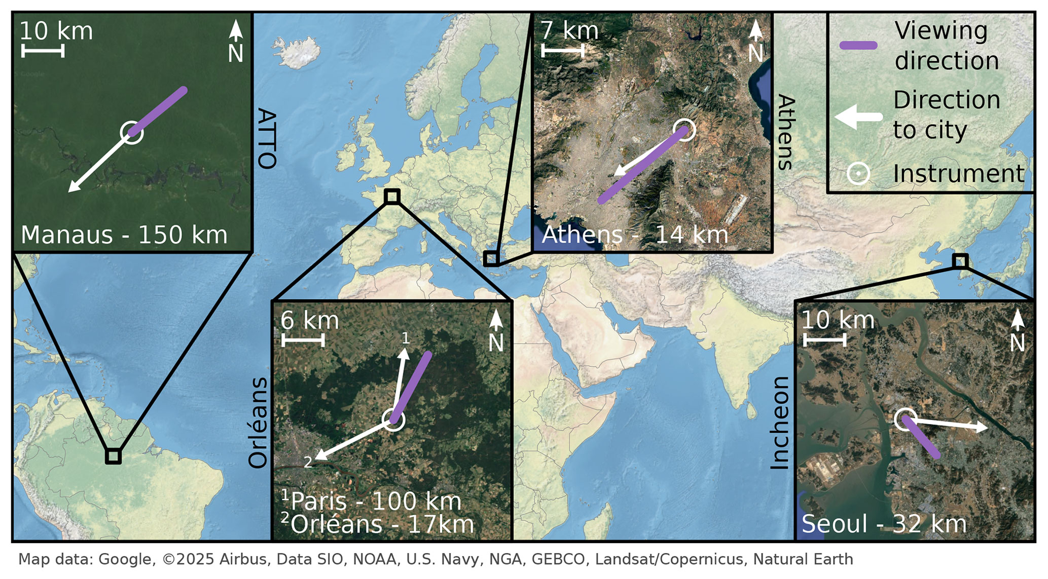
Figure 1Map showing the location of all stations, their surroundings and distances to neighbouring cities. The white circles indicate the instrument positions, the white arrows show the direction to the city centres, whereas the purple lines correspond to the relevant viewing direction of the instruments.
Table 1Station information overview.
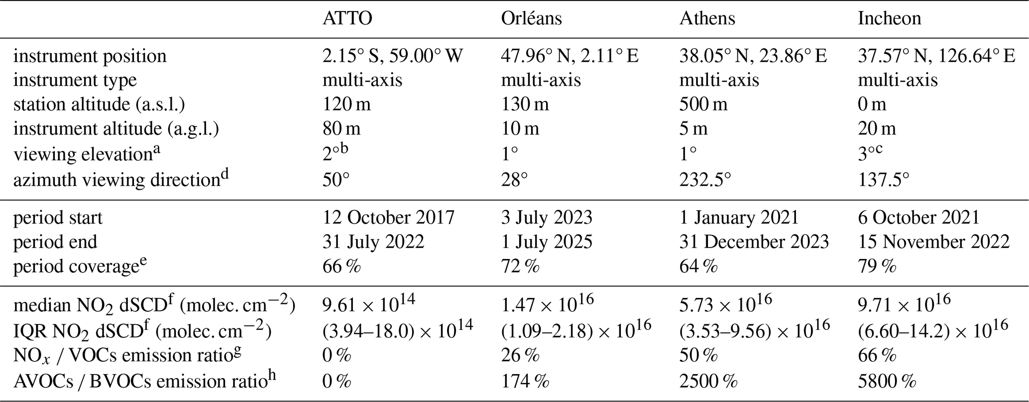
a The supplement also contains figures with data from 30° viewing elevation.
b The highest O4 dSCDs occurred for 2° elevation.
c Lower elevations are obstructed.
d N = 0° and E = 90°.
e Days with observations after filtering and merging (intersect) of all trace gases.
f From viewing elevation.
g Based on area weighted annual average CAMS-GLOB-ANT emissions and CAMS-GLOB-BIO emissions during measurement years (excluding 2025 for Orléans).
h Ratio of anthropogenic non-methane VOCs (AVOCs) emissions from CAMS-GLOB-ANT to biogenic non-methane VOCs (BVOCs) emissions from CAMS-GLOB-BIO.
The third station, Orléans, is classified primarily as a biogenic environment. This classification is supported by relatively low observed median NO2 levels, and a viewing direction aimed directly over forest canopies. The fourth station, ATTO, is similarly considered biogenic, given its remote location within the Amazon rainforest. Potential pyrogenic influences at ATTO (wildfires during the dry season) and Athens (occasional wildfires) are neglected, as we expect such events to influence our measurements only infrequently during our measurement periods.
2.2.1 Athens
The instrument in Athens is located at the National Observatory of Athens in Penteli, Greece. The Athens metropolitan area, with approximately 3 million inhabitants in the Attica region (Hellenic Statistical Authority, 2024), is strongly influenced by anthropogenic activity. Under certain meteorological conditions, local topography causes pollutants to accumulate within the urban area (Kassomenos et al., 1995). Additionally, due to its hot and dry climate, Athens occasionally experiences wildfires, as observed, for example, in 2018 and 2024 (Lagouvardos et al., 2019; Castro-Melgar et al., 2025). Mountains with Mediterranean vegetation are located to the north. To the east, the landscape features mountainous vegetation interspersed with smaller residential areas, while to the south lie the airport and lower-density residential and industrial zones. The city centre of Athens and the port of Piraeus are situated to the southwest.
The MAX-DOAS instrument is installed on a building roof on a hill (500 m above sea level; a.s.l.) to the east of the city (see Fig. 1). Measurements are routinely conducted in multiple directions. For this analysis, we use data collected between January 2021 and December 2023 from the viewing direction oriented toward the city centre (indicated by the purple line in Fig. 1). Additional details regarding the instrument hardware and setup are given by Gratsea et al. (2016). Meteorologically, the region experiences low precipitation, pronounced diurnal and seasonal cycles in short-wave radiation, and relatively high temperatures exhibiting clear seasonal and daily variations during our measurements (Fig. 2). The prevailing winds during the measurement period come from northern directions, frequently reaching speeds above 9 m s−1 (Fig. S2).
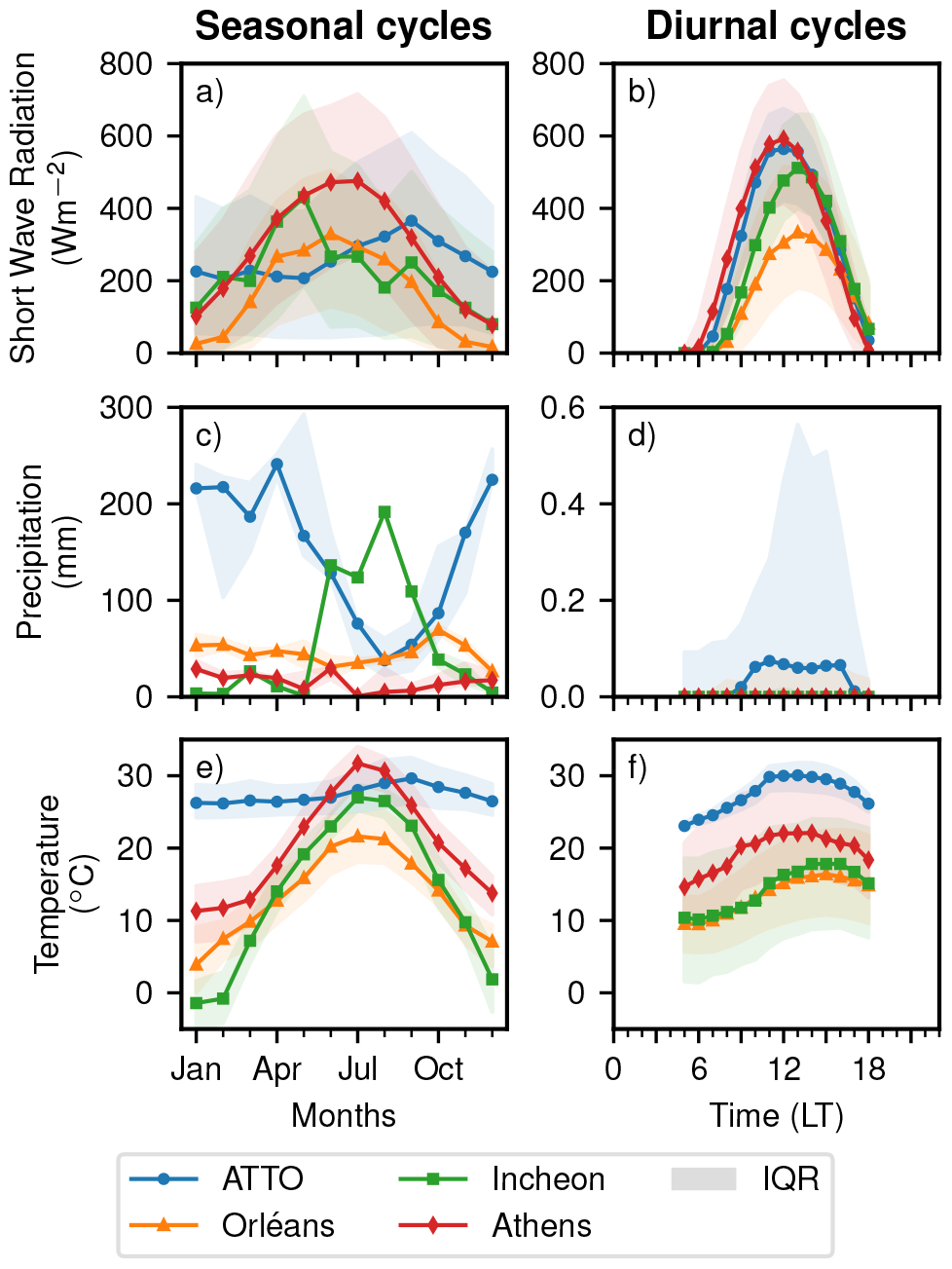
Figure 2Meteorological overview showing the seasonal cycles (left column) and the diurnal cycles (right column) of median short wave radiation (first row), median monthly/hourly sum of precipitation (second row) and median temperature (third row) for the analysed stations based on ERA5 data. The shading corresponds to the interquartile range (IQR). To closely describe the conditions during measurements, only data during daytime, between 05:00 and 18:00 local time (LT), are considered during the sites operation years.
2.2.2 Orléans
The second station is located near Orléans, France, on the premises of a radio station in Traînou, which is regularly used for scientific measurements, including the ICOS project (Ramonet et al., 2025). Traînou (approx. 3500 inhabitants; Institut national de la statistique et des études économiques, 2025) is situated about 100 km south of Paris and 17 km northeast of Orléans (116 000 inhabitants; Institut national de la statistique et des études économiques, 2024).
Crucially for this study, the site is adjacent to a large forested region (Fig. 1). The Orléans State Forest covers roughly 350 km2, and comprises a mixture of broadleaf and evergreen tree species (Bello et al., 2019). Thus, this measurement site is strongly influenced by biogenic activity, with minimal local anthropogenic emissions, although pollutant plumes from Paris can occasionally be detected under northerly winds.
The MAX-DOAS instrument is mounted on an elevated position (approx. 10 m above ground level; a.g.l.), enabling low-elevation scans directly above the forest canopy. Data analysed in this study cover the period from July 2023 to July 2025, focusing on measurements taken towards the forest (Fig. 1). Orléans experiences strong seasonal and diurnal variations in short-wave radiation, though its maximum values are comparatively low due to its higher latitude (Fig. 2). Precipitation is moderate without a clear seasonality. Temperatures are among the lowest of the investigated sites, with a less pronounced seasonal cycle than at Incheon and Athens. The prevailing wind direction is from the southwest, frequently exhibiting high wind speeds exceeding 9 m s−1 (Fig. S2).
2.2.3 Incheon
The third instrument was installed on the roof of the Environmental Satellite Center in Incheon, part of the Seoul Metropolitan Area (SMA) in South Korea. With approximately 3 million inhabitants, Incheon is South Korea's third-largest city. The SMA is the most densely populated region in the country (Kim et al., 2021). It is situated in an anthropogenically dominated environment, with Seoul city centre approximately 32 km to the east, Incheon city centre to the south, and the harbour area to the west (Fig. 1). The northern edge of the metropolitan area borders North Korea (about 20 km north), where some forested mountains are located.
As part of the GEMS Map of Air Pollution (GMAP) 2021 campaign and the Satellite Integrated Joint Monitoring of Air Quality (SIJAQ) 2022 campaign, MAX-DOAS measurements were conducted for about one year. For this study, we analyse data from October 2021 to November 2022, focusing on the urban azimuth viewing direction.
Meteorologically, heavy rainfall occurs between June and September, while the rest of the year is comparatively dry. This signal indicated the influence of the East Asian monsoon and tropical cyclones. No pronounced diurnal precipitation cycle is observed. The seasonal precipitation pattern affects short-wave radiation, which declines during the wet months but otherwise shows strong seasonal and diurnal cycles with high peak values. Temperatures also exhibit strong seasonal and diurnal variability, with the lowest temperatures across all sites recorded in December and January. The prevailing wind direction is from the northwest (especially during Winter) or west (Fig. S2).
2.2.4 ATTO
The fourth instrument is located on the tall ATTO Tower in Brazil, deep within the Amazon rainforest. Situated approximately 150 km northeast of Manaus (population 2 million, Instituto Brasileiro de Geografia e Estatística, 2022), the ATTO site serves as a remote research site in the heart of the rainforest (Fig. 1). The surrounding area is sparsely populated, resulting in the site being predominantly influenced by biogenic activity. During the dry season wildfires are more frequent and affect local atmospheric conditions (Andreae et al., 2015; Donner, 2024).
The instrument was installed at a height of 80 m in October 2017 and measurements are still ongoing at the time of writing. However, not all data are yet analysed in scientific quality, so the used dataset ends in August 2022. Some data gaps occurred due to the challenging hot and humid climate affecting hardware and electronics. The dataset analysed in this study was originally obtained by Donner (2024), who also provides a detailed description of the site and instrumentation. Some figures from that publication are reproduced here using our own processing methodology based on their dataset. In such cases, the figure captions indicate which panels are affected.
Meteorologically, the ATTO Tower is characterised by a tropical climate, see Fig. 2. Precipitation is largely confined to the wet season (December–May), with much drier conditions prevailing during the rest of the year. Within this season, rainfall typically occurs between 10:00 and 16:00 LT. Temperatures are consistently high, showing daily but minimal annual variation. Short-wave radiation exhibits a strong diurnal pattern but remains relatively stable on seasonal timescales, with only a slight reduction during the wet season. Prevailing winds are from the northeast, but compared to the other sites, wind speeds are predominantly low, typically below 3 m s−1 (Fig. S2).
2.2.5 Coverage and representativeness
The four stations cover a broad range of environmental conditions; however, they cannot represent the full diversity of atmospheric regimes. In particular, both urban sites, Incheon and Athens, are located near the coastline, implying potential influences from marine air masses and sea-salt aerosols that may not be representative of inland urban environments. The datasets were collected during non-overlapping periods, as the station locations originate from long-term measurement activities. While this limits strict temporal comparability, the analysis focuses on characteristic relationships rather than direct year-to-year contrasts.
The horizontal orientation of the light paths introduces an additional spatial averaging that is inherent to MAX-DOAS measurements and is illustrated in Fig. 1. The retrieved dSCDs represent the concentration along the effective light path, whose length within the boundary layer depends on atmospheric visibility. Under clear conditions, photons scattered at distances of up to approximately 15 km from the instrument can contribute to the signal (Seyler et al., 2017).
Beyond viewing geometry, the origin and transport history of observed air masses determine the spatial representativeness of each site. Annual and seasonal horizontal footprints derived from backward simulations (details in Sect. 2.4) show, as expected, the highest sensitivity in the vicinity of each instrument (Fig. 3). The ATTO footprint shifts seasonally with the movement of the ITCZ. At Orléans, persistent sensitivity to both the city and the surrounding forest reflects mixed anthropogenic and biogenic influences, with enhanced sensitivity towards Paris (100 km to the northeast) during MAM. Athens exhibits strong sensitivity to the urban area and more remote northern regions, with reduced sensitivity to the city centre and harbour in JJA. Incheon shows pronounced sensitivity to northwestern source regions during DJF, with a less directional footprint in the remaining seasons. Overall, the footprint analysis is consistent with the site descriptions and classifications, but reveals minor seasonal sampling biases that should be considered when comparing sites.
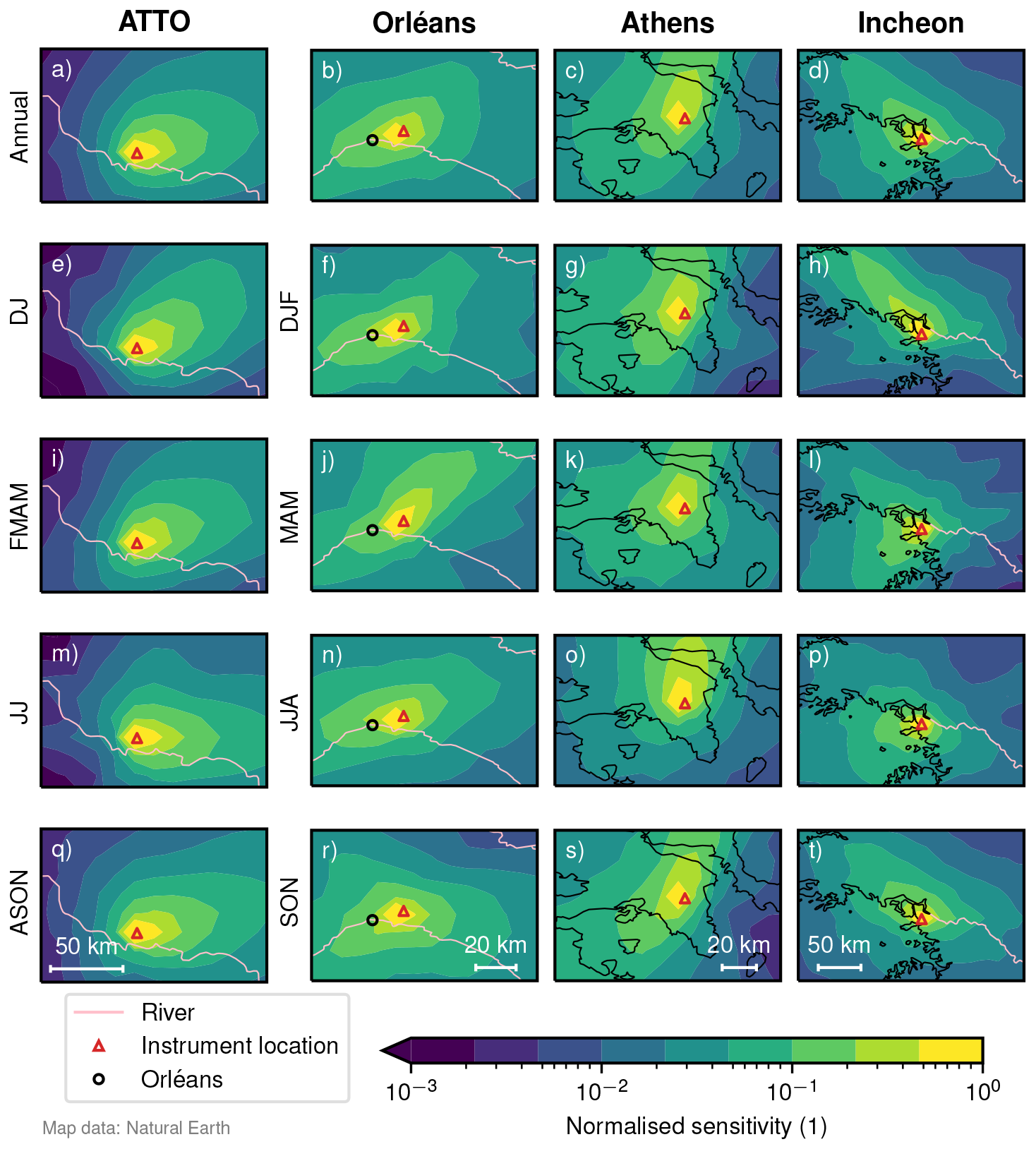
Figure 3Annual and seasonal station footprints, based on normalised sensitivity with respect to the maximum per panel. The annual distribution is shown in the first row, and the seasonal distributions are shown in the rows below. Note that the months for ATTO are grouped differently to account for wet (FMAM) and dry (ASON) season.
2.3 Computation of RGF
We calculate RGF for each pair of corresponding quality-filtered CHOCHO and HCHO dSCDs. Since CHOCHO and HCHO are retrieved in different spectral ranges, atmospheric scattering processes, such as Rayleigh scattering, vary, resulting in different effective light path lengths (Seyler et al., 2017). This discrepancy can introduce systematic differences between the two dSCDs, as each trace gas effectively samples a slightly different part of the boundary layer.
To estimate and correct for differences in light path lengths, we use the collision-induced absorption of O2–O2, typically approximated as O4, which must be included as an absorber in DOAS retrievals (Finkenzeller and Volkamer, 2022). The vertical profile of O4 is well characterised; its VCD can be accurately calculated because O2 concentration decreases approximately exponentially with altitude, producing a known vertical distribution of O4. We apply a first-order correction by multiplying RGF with the inverse of the O4 dSCDs from the corresponding wavelength regions, see Eq. (3). This correction approach is effective because the O4 VCD cancels out in the process, leaving only the ratio of the respective air mass factors (AMF, AMF), which accounts for differences in physical processes, see Eq. (4).
The O4 correction assumes that the vertical profiles of CHOCHO and HCHO closely resemble that of O4, since the O4 AMF is used to correct for differences in effective light path length (Sinreich et al., 2013). This assumption is reasonable for our dataset, as we focus on the lowest elevation angles, where slant columns are dominated by near-surface absorption. However, when the profiles of CHOCHO and HCHO deviate from the exponential O4 profile, the accuracy of the correction decreases. Such deviations may arise, for example, from enhancements at elevated layers due to fire plumes, or from a box-shaped profile under conditions of strong atmospheric stratification.
Overall, the O4 correction of RGF is important for interpreting the results because the physical processes, influencing the effective light path, are systematically different in the spectral ranges of CHOCHO and HCHO. Since dSCDs are used to compute RGF, if left uncorrected, these light path effects alter the values of RGF, hiding the influence of the actual drivers. Figure 5 (bottom row) illustrates the impact of the correction. The O4 ratio is relatively constant over the day and primarily reduces the overall magnitude of the corrected RGF. Throughout this study, we denote the uncorrected glyoxal-to-formaldehyde ratio as RGF and the O4-corrected ratio as . Changes in are expressed in % for relative changes and in %pt. for absolute changes.
The O4 dSCDs used for correction are obtained from the respective NO2 fits in the visible and UV ranges for the Bremen and MPIC instruments. As the MPIC instrument does not cover the O4 absorption band at 477 nm, the quality of O4 dSCDs in the visible is reduced. Comparing the O4 UV and vis dSCDs for all sites in Fig. 4, shows that the original data from ATTO (Fig. 4a) deviates from the other stations. We primarily attribute the higher slope to the lower quality of the O4 retrieval in the visible. To remove this systematic bias for ATTO in our study, we scale the O4 vis dSCDs of ATTO by using the data from all other sites (Orl+Ath) as the reference. A slope is computed for the original dataset (mATTO, Fig. 4a), and the reference dataset (mref, Fig. 4c). Both slopes are then used to scale the O4 vis dSCDs, see Eq. (5), which yields a more consistent behaviour for ATTO (Fig. 4b). This scaling affects the magnitude of the O4 ratio and makes it comparable with the other sites (Fig. 5m). A comparison of the original and scaled O4 ratio for the other figures is found in Fig. S14.
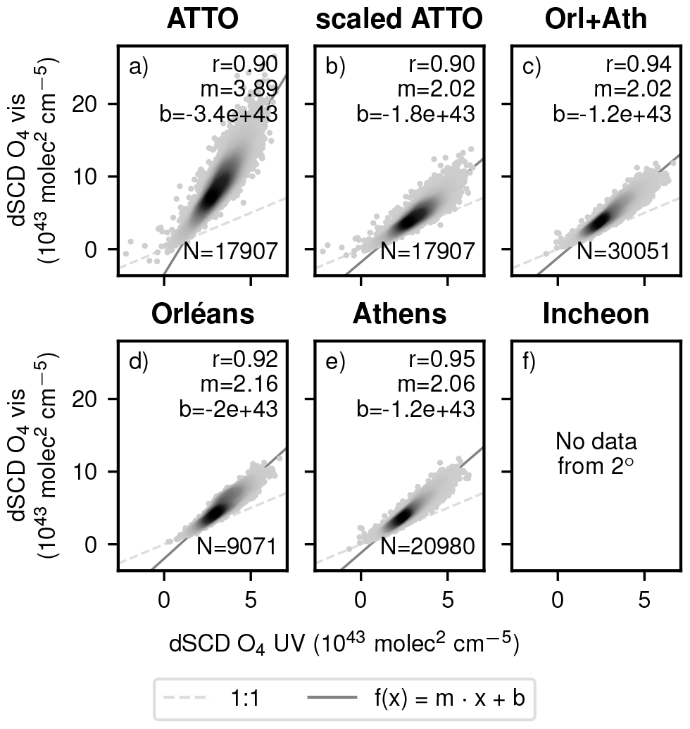
Figure 4O4 vis dSCDs as a function of O4 UV dSCDs for different datasets at 2° viewing elevation. The light grey dashed line indicates the 1-to-1 line and the gray solid line indicates a orthogonal linear fit with the specified parameters. The density of the data points is indicated by the hue, denser regions are shown in darker grey.
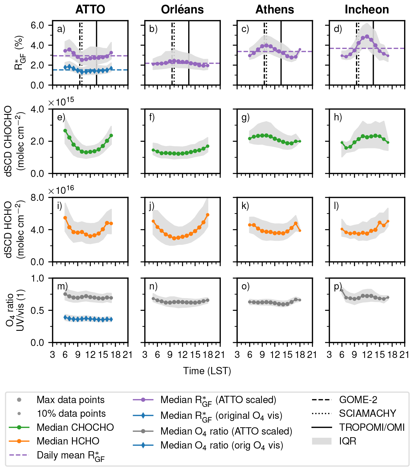
Figure 5Diurnal cycles of (top row), CHOCHO dSCD (upper centre row), HCHO dSCD (lower centre row), and O4 ratio (bottom row) for ATTO, Orléans, Athens, and Incheon relative to local solar time (LST). Marker size scales with the number of contributing observations, with smaller markers indicating fewer measurements. The original and O4 ratio without scaling O4 vis dSCDs is shown for ATTO in blue with diamond markers. In addition, the overpass times of GOME-2, SCIAMACHY and TROPOMI/OMI are highlighted with black vertical bars. Panels (e) and (i) are self-created based on Donner (2024).
Uncertainties of RGF
Uncertainties from MAX-DOAS data can be grouped in (1) random effects and (2) systematic effects. Following the error budget discussion from Pinardi et al. (2013) for the HCHO retrieval from MAX-DOAS data, random uncertainties are connected to photon shot noise for silicon based detectors and are generally well captured, if not even overestimated, in the dSCD uncertainties from the DOAS fit. For scientific grade instruments, the systematic uncertainties outweigh the random uncertainties. Pointing misalignments, uncertainties of the wavelength calibration, and the uncertainties in the retrieval are common sources for systematic uncertainties (Roscoe et al., 2010; Pinardi et al., 2013). These amount to around 20 % for HCHO (Pinardi et al., 2013) and are typically not included in dSCD uncertainties.
Systematic differences in data collection and processing between sites are unavoidable. The instruments do not share identical hardware, and ATTO, the only instrument operated by the Max Planck Institute for Chemistry, uses slightly different fit settings compared to the other instruments. In addition, the O4 vis dSCDs at ATTO are scaled as described above. At Incheon, viewing elevations below 3° are blocked, thereby reducing sensitivity close to the surface compared to measurements at 1° or 2° elevation. At Athens, the instrument is located at 500 m a.s.l., while the city centre lies near sea level. Under shallow boundary layer conditions, such as in winter, the effective light path may therefore only partially sample the polluted boundary layer, resulting in lower measured columns. However, since CHOCHO and HCHO concentrations peak in summer, when the boundary layer is typically well developed, this effect is expected to be small.
To quantify the uncertainty of RGF, we modify the uncertainty propagation from Vrekoussis et al. (2010) to include the O4 ratio:
with a, b, c, d, sx representing dSCD, dSCD, dSCD, dSCD, and the respective standard error. We use the uncertainties obtained from the DOAS fit to account for random uncertainties. The annual and seasonal median uncertainties of per station are listed in Table S9 in the supplement. The random uncertainties are higher during winter (Orléans, Athens, Incheon) and wet season (ATTO). The relative uncertainties of on an annual scale range from 10 % to 20 % for all stations.
2.4 Auxiliary datasets
We use meteorological data to associate changes in with specific meteorological conditions, thereby extending our understanding of its driving factors. To ensure consistency across all stations throughout the measurement periods, we selected data from the ECMWF Reanalysis v5 (ERA5) dataset. ERA5 provides hourly gridded data (0.25° × 0.25° grid spacing). The meteorological variables included in this analysis are temperature at 2 m, dew point temperature at 2 m, boundary layer height, short-wave radiation, total precipitation, and wind speed and direction at 100 m (Hersbach et al., 2023). To merge the ERA5 data with the MAX-DOAS datasets, the ERA5 datasets are interpolated in time to the timestamp of each measurement. Relative humidity is computed via the Magnus approximation from the temperature and dew point temperature.
To investigate differences in emission sources between the sites, we use the CAMS-GLOB-ANT version 6.2 (Soulie et al., 2024) and the CAMS-GLOB-BIO version 3.1 (Sindelarova et al., 2022) emission datasets created by the Copernicus Atmosphere Monitoring Service (CAMS) and provided by ECCAD (Granier et al., 2019). The data is used in Table 1 characterising the stations by their NOx to VOCs ratio and anthropogenic VOCs to biogenic VOCs ratio. In addition, the anthropogenic contributions of non-methane VOCs for both urban sites during the observations are used to aid interpretation of the –NO2 relationship in Fig. 12. For the respective contributions, the annually gridded CAMS-GLOB-ANT (0.1° × 0.1° grid spacing) for non-methane VOCs and NOx (in Tg) and CAMS-GLOB-BIO (0.25° × 0.25° grid spacing) for all VOC species (in Tg) are summed up over a region enclosing the sites, see Fig. S1. Carbon monoxide, methane, methyl chloride, methyl iodide, methyl bromide, and hydrogen cyanide are excluded for the contributions of biogenic VOCs from CAMS-GLOB-BIO.
To quantify the sensitivity of our measurements to nearby source regions, we performed backward simulations with FLEXPART version 10.4 (Pisso et al., 2019), driven by ERA5 meteorological fields. Hourly footprints were generated by initiating one simulation per hour, each with an 1 h emission pulse and a 3 d backward integration period. Residence times (i.e. sensitivity, in s) were integrated over the full atmospheric column and accumulated over the entire simulation period. The released tracer was configured as a proxy for CHOCHO with a lifetime of 3 h. For each station, we selected 1 representative year in which the annual wind rose closely matched the corresponding multi-year wind rose (see Fig. S9). As the aim of the simulations is to study the spatial distribution of the footprint, only normalised sensitivity with respect to the maximum value is studied here.
2.5 Statistical tests
To assess whether observed differences in mean values are caused by random variability, we apply statistical tests in Sect. 3.1.2 and 3.1.3. Since measurements are available approximately every 30 min, consecutive data points may sample the same atmospheric event. To increase statistical independence, the data are temporally aggregated prior to testing. Where appropriate, a logarithmic transformation is applied to approximate normality.
To compare biogenic and anthropogenic environments, represented by ATTO & Orléans and Athens & Incheon, the data are aggregated to monthly means per station (e.g., 2 years of data yield 24 values) before grouping. The differing seasonal cycles between the Northern and Southern Hemisphere sites inflate intra-group variability, biasing the test conservatively towards non-significance; the reported p value therefore represents an upper bound. Differences between groups are tested using Welch's t test (Welch, 1947; Delacre et al., 2017) applied to the log-transformed data, which accounts for unequal variances and sample sizes. The same aggregation strategy is used for station-to-station comparisons. In this case, a Welch analysis of variance (ANOVA) (Welch, 1951; Delacre et al., 2019) is applied first to the log-transformed data to assess overall differences among stations. It is followed by a Games–Howell post hoc test (Games and Howell, 1976), which evaluates pairwise differences while accounting for unequal variances and sample sizes. To investigate a potential weekend effect, the data are aggregated to weekly means separated into workdays and weekends for each station. Welch's t test is then applied to the corresponding subsets.
3.1 Temporal cycles
3.1.1 Diurnal cycle
A diurnal cycle describes the variation over a day. It allows to compare with other variables that change regularly over the day, e.g. incoming solar radiation or car traffic. For the case of RGF, multiple diurnal cycles were reported. At two sites, one in India (semi-urban) and one in Thailand (rural), Hoque et al. (2018a, b) and Rawat et al. (2024) observed a diurnal cycle with a noon maximum for RGF based on VCDs retrieved from MAX-DOAS measurements. The values ranged from 2 %–4 %. Hoque et al. (2018a) also found the diurnal cycle of RGF to be less pronounced in the dry season compared to the wet season, which we will revisit for ATTO in Sect. 3.1.2.
DiGangi et al. (2012) investigated the diurnal cycle at two predominantly biogenic sites at higher altitudes (Sierra Nevada Mountains, 1315 m; Rocky Mountains 2286 m) with field campaigns in July 2009 and August 2010 utilizing in-situ instruments. The average RGF values for both campaigns were about 2 % and 1.7 %. At the Sierra Nevada site, RGF increased to about 3 % around midday to afternoon. Whereas the Rocky Mountains campaign showed only minor diurnal variability. DiGangi et al. (2012) attributed the observed enhancements primarily to anthropogenic VOCs and biomass burning plumes encountered during the campaigns.
The diurnal cycles of in local solar time (LST) differ strongly across the four stations (Fig. 5). Anthropogenic sites show pronounced diurnal variability, while the biogenic sites show relatively little variation over the day. At ATTO and Orléans, the diurnal cycles are relatively flat. In contrast, Athens and Incheon exhibit higher average values and strong diurnal patterns, with peaks around 10:00 LST in Athens and noon in Incheon. In Athens, the cycle follows morning rush hour, whereas Incheon has a noon maximum, indicating different drivers of over the day for both cities.
The diurnal pattern of is broadly consistent across seasons, although seasonal offsets in the absolute values are present. The largest offset occurs between the wet and dry seasons at ATTO, which is discussed in detail in Sect. 3.1.2. Notably, although the diurnal cycles of HCHO and CHOCHO individually change between seasons, their ratio retains a similar diurnal shape throughout the year (Fig. A1).
Except at ATTO, data availability decreases in the early morning and late afternoon due to the applied SZA filter, which excludes measurements at large SZA. Throughout this study, marker size is scaled to the number of observations per bin; smaller markers therefore indicate reduced bin size. The detailed mapping of bin sizes is provided in the Supplement (Fig. S4). Data from these times of day are mainly collected during summer months, introducing a seasonal bias in the early and late portion of the diurnal cycle. Furthermore, the number of valid data points decreases substantially during the winter months at Orléans, Incheon, and Athens, primarily because we filter by relative error of CHOCHO dSCDs, which increases for low atmospheric concentrations. Filtering by relative error is needed to limit the scatter of , but it means that is more representative for high CHOCHO and HCHO columns.
The effect of scaling the vis O4 dSCDs for ATTO is highlighted again by showing the original data with the blue lines in Fig. 5. The overall high O4 dSCDs in the visible lead to a really low O4 ratio (Fig. 5m), which is mirrored in the overall low level of (Fig. 5a). The O4 ratio, after scaling ATTO, is of similar magnitude across sites and does not contribute to a pronounced diurnal cycle.
Examining the components of in Fig. 5 reveals that CHOCHO behaves differently across the four stations. HCHO dSCDs follow a U-shaped diurnal cycle at all stations, with a maximum in the morning and evening and a minimum around noon. This pattern has previously been attributed to enhanced sinks (photolysis and OH oxidation) dominating around midday (Nussbaumer et al., 2021; Donner, 2024). However, the underlying processes are more complex as they can also promote secondary formation of CHOCHO and HCHO by breaking down VOC precursors.
The diurnal cycle of the CHOCHO dSCDs varies in magnitude and shape across stations. ATTO also shows a pronounced U-shape. Orléans exhibits a relatively flat diurnal cycle. Contrasting to that, the anthropogenic stations show a different behaviour. Here, we find higher daily averages plus a maximum in Athens around 10:00 LST and in Incheon over noon. The shapes of the diurnal cycles at the anthropogenic stations suggest a stronger link to anthropogenic activity for CHOCHO than HCHO. Since direct CHOCHO emissions are suspected to be low (Stavrakou et al., 2009a; Silva et al., 2018), anthropogenically emitted precursors with a high CHOCHO yield might be a possible explanation, like aromatics (Chan Miller et al., 2016) or acetylene/ethylene (Fu et al., 2008). Furthermore, other effects independent from emissions could have an influence, like differences in photolysis, OH loss, heterogeneous uptake, and wet removal, but our dataset does not allow to separate such effects. Resulting different photochemical lifetimes of CHOCHO and HCHO might also contribute to the shape of the diurnal cycle of . Under simplified conditions, a longer lifetime of CHOCHO compared to HCHO, results in an increase of and a decrease otherwise (see Fig. S7).
Considering these curves, the diurnal cycle of appears to be driven by CHOCHO. The enhanced daily mean in Athens and Incheon can be explained by the overall higher CHOCHO levels. The shape of diurnal cycle can be attributed to the behaviour of CHOCHO dSCDs. Similar shapes between CHOCHO dSCDs and HCHO dSCDs lead to flat cycles at ATTO and Orléans, whereas the different shapes of CHOCHO dSCDs and HCHO dSCDs lead to a pronounced diurnal cycle of at the anthropogenic stations.
A direct quantitative comparison with previous studies is complicated by methodological differences: whereas DiGangi et al. (2012) report in-situ point measurements and Hoque et al. (2018a, b) and Rawat et al. (2024) derive RGF from VCDs, our is based on corrected dSCDs, which integrate over a slant light path and are therefore sensitive to a different effective measurement volume (Sect. 3.4.1). Despite this, the qualitative diurnal patterns are broadly consistent. The midday peak observed at Incheon is also reported for rural and semi-urban sites in Southeast Asia (Hoque et al., 2018a, b; Rawat et al., 2024). However, the occurrence of similar patterns across differently classified sites highlights a broader challenge in the literature: the lack of a uniform site categorisation complicates cross-study comparisons of RGF. At our predominantly biogenic sites ATTO and Orléans, the diurnal cycle is comparatively flat, which is consistent with the weak diurnal variability reported by DiGangi et al. (2012) for high-altitude biogenic sites.
In summary, shows enhanced average values over the day for anthropogenic stations, due to enhanced CHOCHO levels. This indicates that contains information about the different environments, which supports its usage as a proxy for VOC origin. The pronounced diurnal cycles for anthropogenic stations, however, complicate the interpretation as the timing of the measurement becomes important. The implications for comparing RGF values of different studies are discussed in Sect. 3.4.3.
3.1.2 Seasonal cycle
The variation over the year, the seasonal cycle, enables to investigate how a variable is connected to changes of other variables based on seasons. Multiple studies have reported seasonal cycles for RGF so far: Hoque et al. (2018a, b) and Rawat et al. (2024) found a relatively flat seasonal pattern at Pantnagar (India, described as semi-urban) based on MAX-DOAS VCDs. At a second site, Phimai (Thailand, described as rural), the seasonal cycle showed an increase from January to September. Similarly, Xing et al. (2025), analysing one year of MAX-DOAS VCDs from Guangzhou (China), found enhanced RGF values from November to April and lower values during the rest of the year.
The overall shape of the seasonal cycle of is similar across all four stations, with one minimum and one maximum per year (Fig. 6). At Orléans, Athens, and Incheon, the lowest values occur in July and August (late summer), while the highest values are observed between October and March (winter). At ATTO, the seasonal cycle is shifted by several months, with a minimum in October (dry season) and a maximum extending into June (wet season). Notably, the minimum phase at the biogenic sites tends to be more prolonged compared to the anthropogenic sites. Fewer data points are available in winter due to filtering based on relative error (see Sect. 3.1.1).
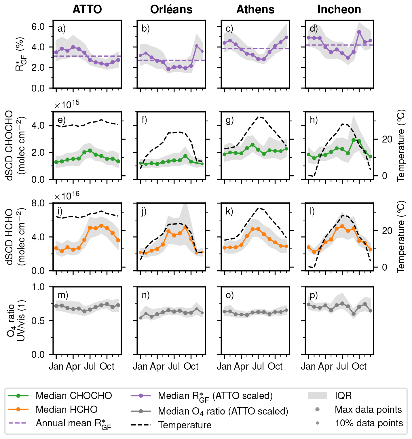
Figure 6Seasonal cycle of (top row), CHOCHO dSCD (upper centre row), HCHO dSCD (lower centre row), and O4 ratio (bottom row) for ATTO, Orléans, Athens, and Incheon. Marker size scales with the number of contributing observations, with smaller markers indicating fewer measurements. The seasonal cycle of temperature is shown on a secondary axis with a dashed black line. Panels (e) and (i) are self-created based on Donner (2024).
Examining the components of separately reveals that both trace gases behave differently for all four stations, whereas the O4 ratio is similar. Looking at the seasonal cycles of HCHO dSCDs we see one enhanced period during the middle of the year, a narrow peak during June and July for Athens, and an extended peak over four months spanning from June to October for the other stations. The annual means and the amplitude are comparable between the stations. The seasonal cycle of CHOCHO dSCDs is relatively flat with one peak in different months from June (Athens) to October (Incheon). One can see a shift to higher annual mean values from ATTO to Incheon. The anthropogenic stations show the highest CHOCHO dSCDs and more variability over the year.
Aggregating all data points by month and grouping them by dominant environment, i.e. Orléans and ATTO as biogenic and Athens and Incheon as anthropogenic, yields mean values of 3.2±1.1 % in the biogenic environment and 4.2 ± 0.8 % in the anthropogenic environment. Looking at mean per station leads to 3.4 ± 0.9 %, 2.7 ± 1.3 %, 3.9 ± 0.8 %, 4.6 ± 0.7 % for ATTO, Orléans, Athens, and Incheon respectively. Applying statistical tests, as described in Sect. 2.5, leads to significant differences (t = −5.8, p = 8 × 10⁻⁸) between the biogenic and anthropogenic group. A Welch-ANOVA (F = 19, p = 3 × 10⁻⁸) combined with a Games–Howell post-hoc test resulted in significant differences for all station pairs except ATTO–Orléans and Athens–Incheon. More detailed results can be found in the Supplement (Tables S6 and S7). It should be noted, that the aggregated data points maintain a significant autocorrelation due to the seasonal cycle.
Three seasonal shifts of the station footprints were identified from Fig. 3 for the non-tropical sites: increased sensitivity toward Paris during MAM at Orléans, reduced sensitivity to the harbour and city centre during JJA at Athens, and enhanced sensitivity to less densely populated regions northwest of Incheon during DJF. None of these shifts is clearly reflected in the seasonal cycle of , suggesting that a simple seasonal categorisation might not be enough to capture clear pathway dependencies (Poulidis and Takemi, 2016).
For all stations except ATTO, the seasonal cycle of HCHO dSCDs closely resembles the seasonal cycle of temperature, which is shown on a second axis in Fig. 6. While temperature variability in ATTO is limited, a slight increase during September–October coincides with peak HCHO values. The seasonal cycle of CHOCHO does not show a clear influence by temperature. This highlights ATTOs unique tropical conditions: the near-constant temperature throughout the year means that seasonal variability in both trace gases is governed by processes other than temperature.
Donner (2024) suggested, that the two trace gases undergo different processing in the dry and wet season and that the seasons probably have a different precursor composition. As reported by Donner (2024), enhanced values in the wet season and reduced values in the dry season are found, see Fig. 7. The daily mean is reduced by 0.7 %pt. in the dry season. The shape of the diurnal cycle is relatively flat. Since forest fires predominantly occur in the dry period, previously excluded pyrogenic activity may contribute to the observed changes. This would be supported by enhanced NO2 levels and aerosols during the dry season as shown by Donner (2024). Since biomass burning has been reported to lead to higher RGF levels (DiGangi et al., 2012; Zarzana et al., 2017; Chan Miller et al., 2014; Alvarado et al., 2020), the observed low median values at this site are unlikely to reflect a significant pyrogenic contribution. Individual pyrogenic events may nonetheless produce enhancements in that are not captured in the median.
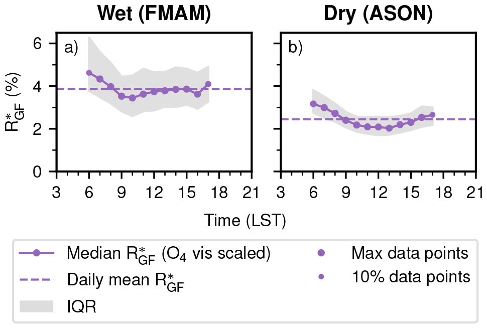
Figure 7Diurnal cycles in the wet (a) and dry (b) season of at ATTO. Marker size scales with the number of contributing observations, with smaller markers indicating fewer measurements.
The discrepancy between wet and dry season is in agreement with the findings of Hoque et al. (2018a), where they found higher RGF during the wet season and lower RGF during the dry season in Phimai (Thailand). Furthermore, both seasons share the same diurnal cycle for Hoque et al. (2018a). However, their diurnal cycle had a pronounced noon maximum, which is not present in this dataset, and might, even though the Phimai site is described as rural, hint at a stronger anthropogenic influence than at ATTO, see Sect. 3.1.1.
Having these points in mind, the seasonal cycle of seems to be driven, contrary to the diurnal cycles, by the variability of HCHO. The variability of HCHO dSCDs is strongly connected to the variability of temperature for non-tropical stations and seems to be connected to the dry/wet season for ATTO. The enhanced annual mean at anthropogenic stations can be explained by overall higher CHOCHO levels.
As with the diurnal cycle, a direct quantitative comparison is complicated by the fact that previous studies derive RGF from VCDs, whereas our is based on corrected dSCDs at the lowest elevation angles, which correspond to a different effective measurement volume (Sect. 3.4.1). With this caveat in mind, the seasonal pattern at our anthropogenically influenced stations resembles most closely the winter enhancement reported by Xing et al. (2025) for Guangzhou. Our absolute values are lower than those reported by Xing et al. (2025), which may partly reflect the difference in measurement volume (dSCD vs VCD) rather than a true difference in RGF. At our more remote stations, the magnitude of is comparable to that reported by Hoque et al. (2018b) for Pantnagar, even though no progressive annual increase is observed like at Phimai.
Chen et al. (2023) published global RGF maps based on the TROPOMI observations for the year 2019. Although our is derived from dSCDs and therefore does not correspond to the exact same measurement volume (Sect. 3.4.1), a comparison of the magnitude of annual means is still meaningful. Extracting RGF values at our measurement sites from their maps for 2019 suggests the following ranking: Incheon > ATTO > Orléans. Athens could not be identified in their maps due to its vicinity to the coastline. Furthermore, Chen et al. (2023) maps show enhanced RGF values during the wet season compared to the dry season at the ATTO site, which is consistent with our observations.
To conclude, we see a similar pattern for seasonal cycles as for diurnal cycles: exhibits a cycle and its average and its amplitude are more pronounced for anthropogenic stations, but this time originating from variations in HCHO. This complicates the interpretation of as a proxy for VOC origin, because many other seasonal effects can contribute to its variation, e.g. temperature, which are difficult to disentangle from changes in VOC origin over the year. Moreover, longer time series are needed for measurement campaigns to avoid sampling biases.
3.1.3 Weekly cycle
As anthropogenic emissions are typically lower on the weekend, the weekly cycles can be used as an indicator for the contribution of anthropogenic emissions (Beirle et al., 2003). Gratsea et al. (2016) reported a weekly cycle in Athens for glyoxal and to a lesser extent for formaldehyde, but only for measurements dominated by urban air.
To our knowledge, no previous study has investigated weekly cycles specifically for RGF, but from the findings of Gratsea et al. (2016), we expect a weekend effect may occur. In Fig. 8, ATTO and Orléans display flat weekly cycles, while the anthropogenic stations show an offset between weekday and weekend. Moreover, as seen and discussed before for diurnal and seasonal cycles, the average value throughout the week is higher for the anthropogenic stations. It should be noted, that for Incheon is reduced not only during the weekend but also on mondays.
For both stations, the mean weekday exceeds the mean weekend value by 0.5 %pt., corresponding to a reduction of approximately 10 % on weekends. Although this relative difference is comparable to our systematic uncertainties, these uncertainties are expected to affect all days uniformly and should therefore not be relevant for the weekend effect. As described in Sect. 2.5, the differences between weekday and weekend are significant for Athens (t = 4.4, p = 2 × 10⁻⁵) and Incheon (t = 2.7, p = 8 × 10⁻³).
For ATTO and Orléans the weekly cycles of both OVOCs are relatively flat and show no weekend effect (Fig. 8). Comparing both OVOCs over the week for the anthropogenic stations, CHOCHO dSCDs show a strong weekend effect for Athens and Incheon. HCHO dSCDs, however, do not show a strong decrease on the weekend, therefore the weekend effect observed for is driven by the weekend effect from CHOCHO dSCDs.
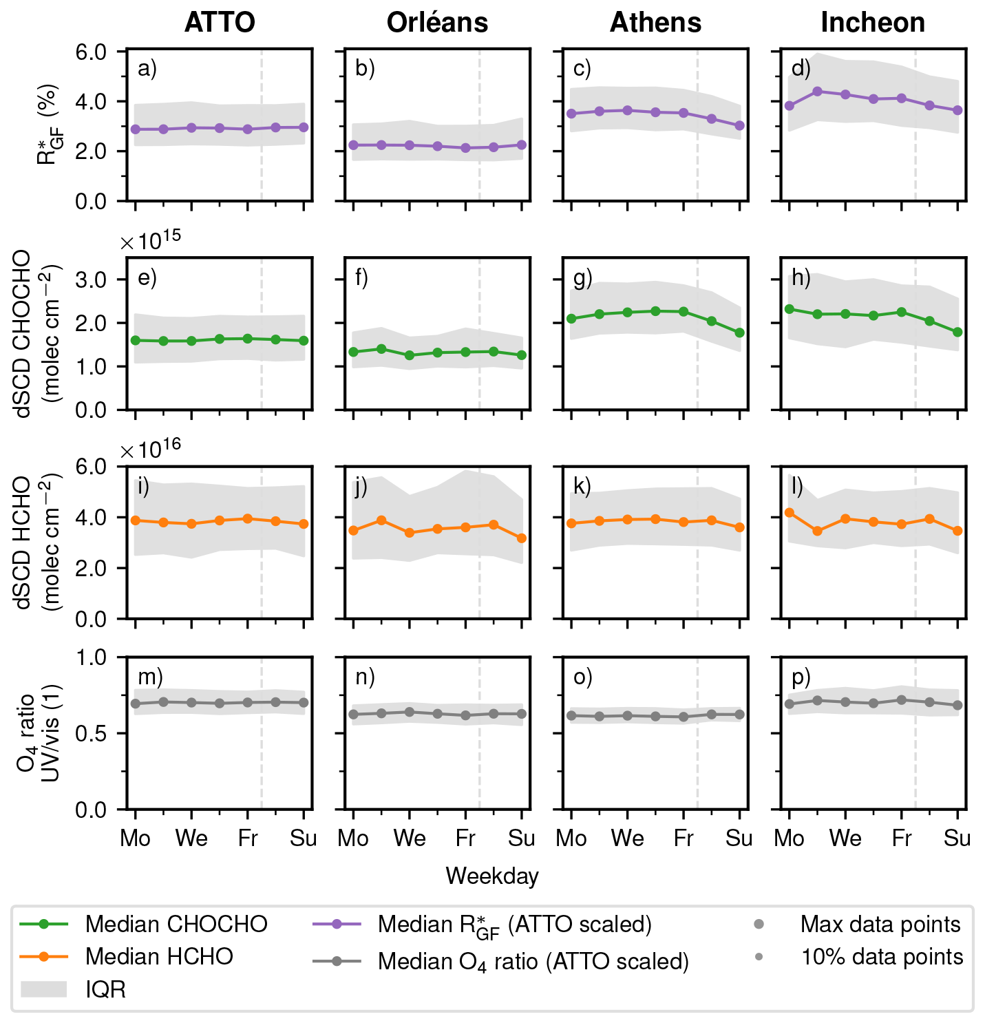
Figure 8Weekly cycle of (top row), CHOCHO dSCD (upper centre row), HCHO dSCD (lower centre row), and O4 ratio (bottom row) for ATTO, Orléans, Athens, and Incheon. Marker size scales with the number of contributing observations, with smaller markers indicating fewer measurements.
To summarize, exhibits a weekend effect for anthropogenic stations, driven by the weekend effect of CHOCHO dSCDs. Showing a weekend effect supports usage as a proxy for different VOC origin, as changes in anthropogenic emissions are mirrored in .
3.2 Link to meteorology
Atmospheric levels of VOCs are known to be influenced by temperature (Pusede et al., 2014; Bourtsoukidis et al., 2024; Li et al., 2024), which could also impact RGF. In addition to temperature, several meteorological factors could theoretically affect RGF. For example, enhanced photolysis rates under higher short wave radiation may alter production and loss pathways, while increased aerosol liquid water content could enhance aerosol uptake and wet deposition of CHOCHO. We use ERA5 meteorological data to examine the dependence of RGF on temperature, dew point temperature, relative humidity, boundary-layer height, short wave radiation, and wind speed.
Although exhibits variability with each of these parameters (Fig. A3), the meteorological variables are strongly intercorrelated, preventing a clear attribution within our dataset. Further, analysing the median for different bins of temperature and moisture content (represented by dew point temperature) shows primarily variation of with temperature (Fig. A4). Given the range of processes directly linked to temperature, such as biogenic emissions and temperature-dependent secondary formation rates, we expect the temperature to be the dominant contributor to the variability of .
3.2.1 Temperature dependence
Few studies have investigated meteorological influence on RGF until time of writing. Guo et al. (2021), who analysed long-path DOAS measurements in Shanghai during summer, mentioned an increase of RGF with temperature over their campaign period. The temperature dependence of exhibits a similar pattern across all stations (Fig. 9): at lower temperatures, values remain relatively stable with some fluctuations. However, starting from about 15 °C, decreases with a maximum reduction of up to 1.9 %pt. observed at Athens. The O4 ratio does not vary with temperature. Looking at HCHO dSCDs it is visible, that the HCHO levels grow exponentially with increasing temperatures across all stations. CHOCHO dSCDs also rise with temperature, most clearly visible for Orléans and way less pronounced for ATTO, Athens, and Incheon.
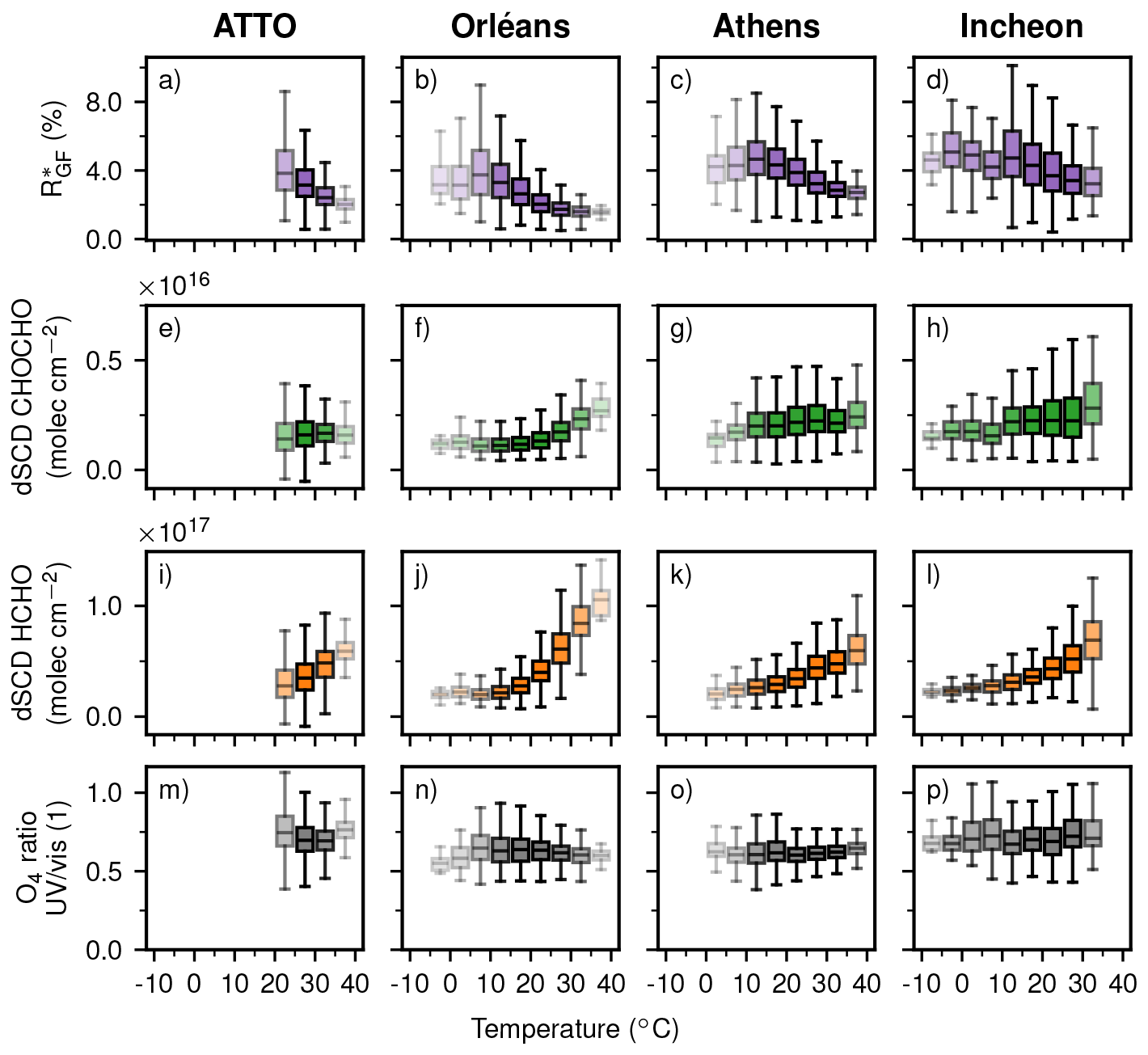
Figure 9 (top row), CHOCHO dSCD (upper centre row), HCHO dSCD (lower centre row), and O4 ratio (bottom row) as a function of binned temperature for ATTO, Orléans, Athens, and Incheon. Within each box, the horizontal line indicates the median and the box spans the IQR; whiskers extend to 1.5 IQR. Box transparency scales with the number of contributing measurements, with more transparent boxes indicating fewer observations. Missing box plots indicate that no data points fall within that interval. Panels (e) and (i) are self-created based on Donner (2024).
An exponential behaviour is expected, especially for the biogenic stations, as biogenic emissions of precursors are known to increase exponentially with temperature (Guenther et al., 1993, 2012; Bourtsoukidis et al., 2024); higher temperatures enhance biogenic activity, which in turn leads to greater VOC emissions. In addition, the secondary formation via OH oxidation should increase with temperature as reaction rates rise (Berg et al., 2024).
For the anthropogenic stations, the situation is different. Here, we expect the anthropogenic emissions to be temperature independent and attribute the exponential increase with temperature primarily to the increased secondary formation at high temperatures. Adding to that, recent studies suggest that local biogenic VOC emissions in urban environments may play a more important role in local atmospheric chemistry than previously assumed (Liaskoni et al., 2024; Wang et al., 2025). It is noteworthy that both trace gases do not behave identically at the anthropogenic stations. All above named arguments, increased secondary formation or potential local biogenic sources, hold for HCHO and CHOCHO, therefore, an important piece of information is still missing.
To summarize, decreases with higher temperatures in our dataset, which is driven by the strong exponential increase with temperature of HCHO. Similar to the other sections, this complicates the interpretation of RGF as a proxy for VOC origin, as the values depend on temperature regardless of the environment of the sites. This has to be considered in the interpretation of when using simple thresholds.
3.2.2 Accounting for temperature dependence
As shown in the previous section, exhibits a strong dependence on temperature in our dataset. To isolate the variability not associated with temperature, we apply a regression-based correction to remove the temperature-correlated component. Specifically, deviations of from its arithmetic mean are fitted using an outlier-robust orthogonal linear regression. Influence from residuals exceeding two standard deviations from zero is reduced by applying linear weighting beyond this threshold. The fitted temperature-dependent component is then subtracted from the dataset.
After removal of the fitted component, the temperature-normalised (Fig. 10e–h) shows only weak dependence on temperature. The diurnal cycles remain largely unchanged by the temperature correction, apart from a slightly reduced amplitude. In contrast, the seasonal variability is substantially reduced at all non-tropical sites, where the seasonal cycle nearly vanishes. At ATTO, however, the seasonal cycle persists, consistent with the comparatively small seasonal temperature variability in the tropics. Revisiting the remaining meteorological variables using the temperature-normalised shows that most of the previously observed variability disappears (see Fig. A2). This is consistent with the strong intercorrelations among the meteorological variables, indicating that the temperature-driven component can account for most of the variability seen for the other parameters.
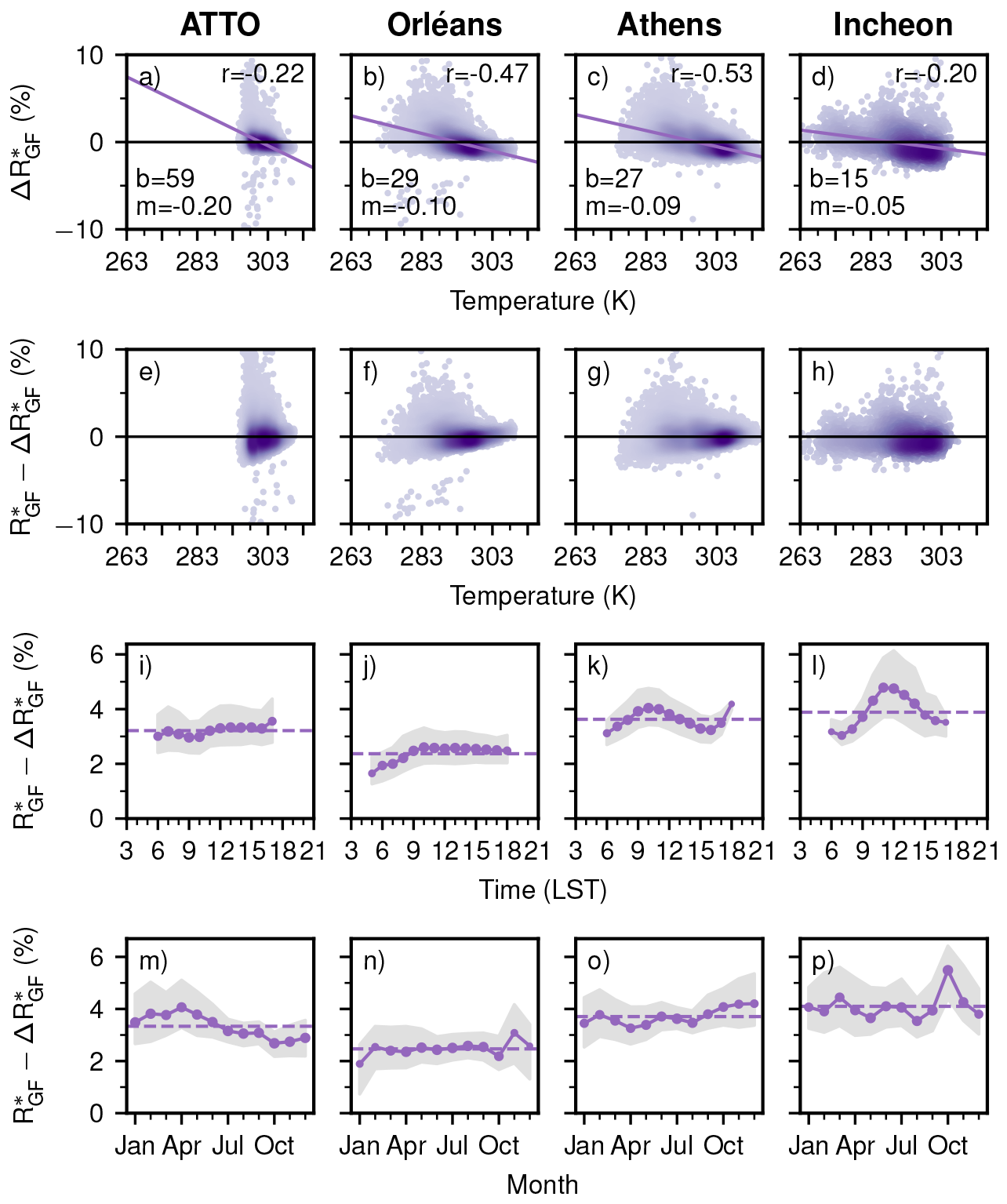
Figure 10Panels (a) to (d) show deviation from the arithmetic mean and the respective regressions. Panels (e) to (h) show the temperature-normalised as a function of temperature. Panels (i) to (l) show the diurnal cycle and panels (m) to (p) the seasonal cycle for the temperature-normalised .
Overall, removing the temperature-driven component largely eliminates both the apparent dependence of on other meteorological variables and the seasonal variability at the non-tropical sites. This suggests that temperature, or processes closely coupled to it, accounts for most of the observed seasonal variability in , while playing a lesser role in driving diurnal variability.
3.3 RGF–NO2 relationship
To assess the use of RGF for VOC source discrimination, it is important to examine how RGF responds to changes in NO2 levels, as NO2 serves as a good indicator of anthropogenic activity. Several studies investigated the NO2 dependency in the past with different results. Vrekoussis et al. (2010) using GOME-2 satellite data reported a clear link between RGF and NO2 levels, with lower RGF values found in polluted environments. Other studies supported this finding, e.g. Hoque et al. (2018a) using VCDs from MAX-DOAS in Phimai (Thailand), Xing et al. (2020) using VCDs from MAX-DOAS in Chongqing (China), and Hong et al. (2024) using VCDs from MAX-DOAS in four megacities (China). Chan Miller et al. (2017), however, observed no clear dependence on NO2 levels using in-situ data from the flight-days with the SENEX aircraft. Another study, by Chen et al. (2023), using TROPOMI satellite data, even reported the opposite trend, where RGF increased with NO2 levels.
Looking at Fig. 11, the four stations span a wide range of NO2 dSCD values, from 1014 to 1018 molec. cm−2. does not show a consistent behaviour across all stations and can be broadly grouped in two categories: stations where no clear correlation between and NO2 is observed (ATTO and Incheon) and stations where increases with higher NO2 dSCD (Orléans and Athens).
Both HCHO and CHOCHO increase with NO2 for the first group (ATTO and Incheon), and this effect cancels out in the . For the second group, we see a different behaviour in each station. In Orléans, HCHO dSCDs decrease with higher NO2 levels, and therefore, increases. In Athens, CHOCHO dSCDs increase more rapidly with higher NO2 levels compared to HCHO dSCDs resulting in increasing at high NO2 levels.The differing behaviour of the two anthropogenic stations, Athens and Incheon, is noteworthy. Despite both being urban environments, responds differently to NO2, which contradicts the expectation that should serve as a consistent proxy for VOC origin. The key difference in our dataset is that CHOCHO dSCDs increase more rapidly with NO2 in Athens than in Incheon.
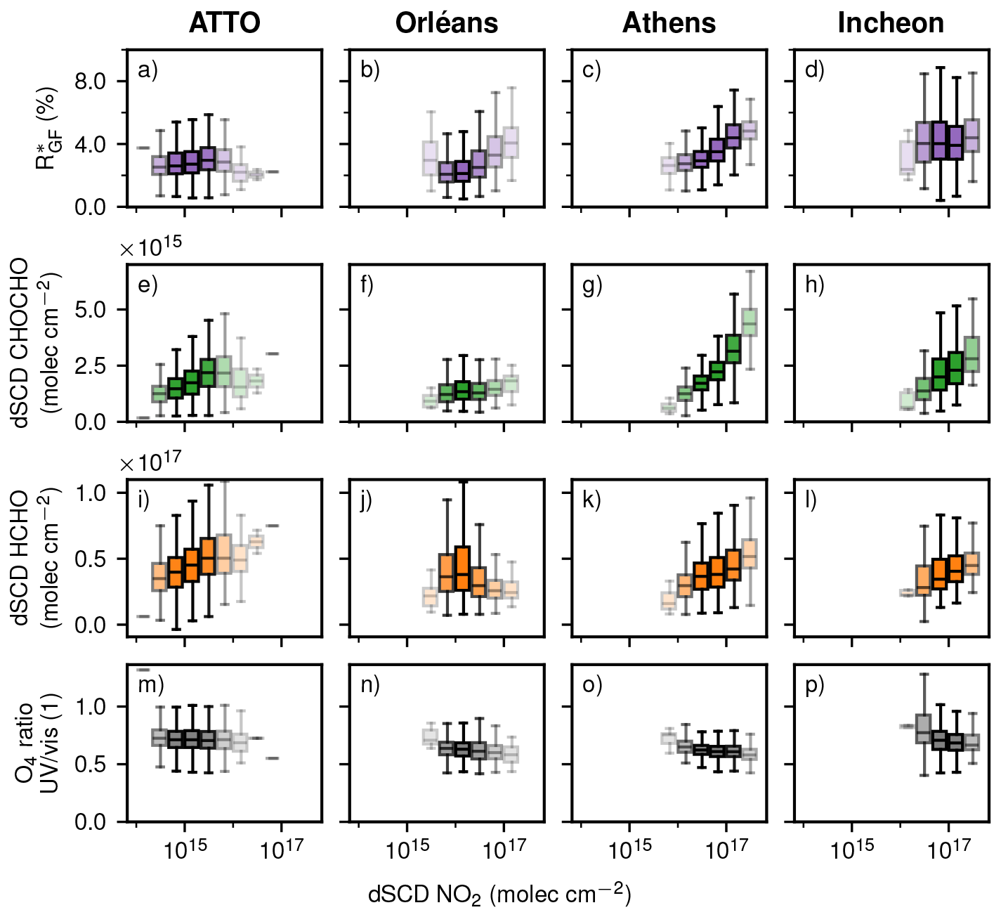
Figure 11 (top row), CHOCHO dSCD (upper centre row), HCHO dSCD (lower centre row), and O4 ratio (bottom row) as a function of binned NO2 dSCDs for ATTO, Orléans, Athens, and Incheon. Within each box, the horizontal line indicates the median and the box spans the IQR; whiskers extend to 1.5 IQR. Box transparency scales with the number of contributing measurements, with more transparent boxes indicating fewer observations. Missing box plots indicate that no data points fall within that interval. Panels (e) and (i) are self-created based on Donner (2024).
In general, increasing NOx concentrations enhance the formation of HCHO and CHOCHO by promoting the recycling of HOx radicals (), which increases OH concentrations and thus strengthens the oxidation of VOCs. This leads to higher production of both species (Seinfeld and Pandis, 2006). The intrinsic yield of CHOCHO and HCHO from VOC oxidation pathways is generally independent of NOx meaning that should remain constant assuming that all ambient factors are the same (e.g., VOC composition, temperature, solar radiation, vertical mixing). However, in high-NOx environments, NOx can suppress OH (through the reaction ), reducing the overall oxidation capacity. This may limit the production of both HCHO and CHOCHO, but depending on their reactivity, this could lead to an increase in even if production is reduced.
The discrepancy between Athens and Incheon hints at a different VOC mixture at each location. In Athens, CHOCHO dSCDs increase more rapidly with NO2 than HCHO dSCDs. A different VOC composition translates via OH-initiated oxidation, followed by reaction with NO, to formation of different alkoxy radicals (RO). The fragmentation of these radicals depends on their structure: larger alkoxy radicals (e.g., from VOCs like aromatics or alkenes) can fragment into both CHOCHO and HCHO. Contrary, smaller alkoxy radicals (e.g., from methoxy, CH3O) produce only HCHO. It should be noted that glyoxal is primarily formed from VOCs with double bonds (C=C), such as aromatics, alkenes, and isoprene. Therefore, higher CHOCHO production relative to HCHO (and thus higher ) suggests a greater contribution from VOCs that produce glyoxal, such as aromatics or unsaturated hydrocarbons, rather than simple alkanes.
Checking the top five sectors contributing to the total non-methane VOCs emissions in both cities from CAMS-GLOB-ANT (Fig. 12) shows similar contributions from solvents and road transport but differences in other sectors. Industrial processes dominate in Incheon, whereas refineries and fugitive emissions are more prominent in Athens. Assuming a consistent VOC composition per sector, regardless of the location, the higher CHOCHO emissions in Athens imply that emissions from refineries and fugitive emissions would produce more CHOCHO relative to HCHO than industrial emissions. Possible species with high CHOCHO yields include aromatics (Chan Miller et al., 2016) or acetylene/ethylene (Fu et al., 2008). However, for aromatics, Nishino et al. (2010) found that CHOCHO yield decreases with increasing NO2 levels. There is also the possibility, that the declining NO2 levels in Incheon (Seo et al., 2021) during the measurement period lead to a more stable RGF–NO2 relationship. But as the Incheon dataset only covers 1 year, the effect should be minimal.
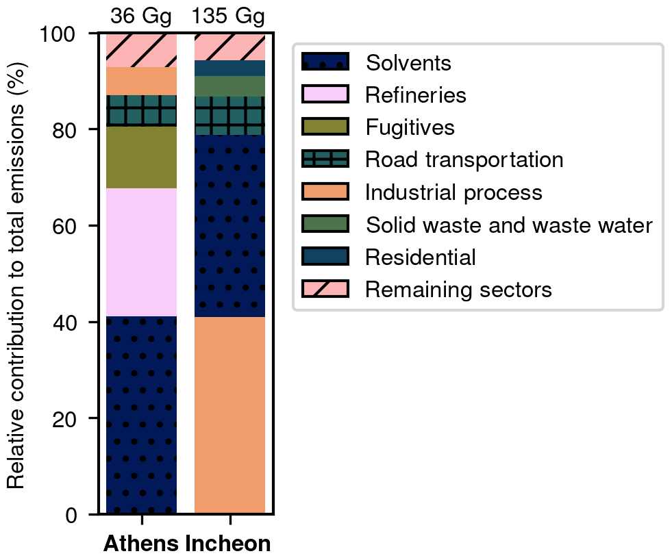
Figure 12Relative contributions to the CAMS non-methane VOCs emissions of the top 5 sectors in Athens and Incheon. All remaining sectors are summarized in one element. The color map is taken from Crameri et al. (2020).
To summarize, shows an inconsistent behaviour with changing NO2 levels and differs between anthropogenic sites. This implies that (1) systematic differences cannot be reduced only to differing NO2 levels; carries additional environmental information. And (2) local factors strongly influence , so using it as a proxy for VOC sources likely requires site-specific considerations.
3.4 Comparability between different RGF
3.4.1 Measurement volume
RGF has been computed from data gathered by various different platforms and with different measurement techniques since its first usage. Table 2 lists the various approaches to compute RGF: volume mixing ratios (VMRs), dSCDs with correction terms, and mean VCDs. All these quantities represent RGF in a different measurement volume. For the particular case of VMR RGF and satellite column-averaged RGF, DiGangi et al. (2012) discusses possible causes for disagreements and also briefly mentions the topic of different measurement volumes. We want to further generalize and expand on this inherent difference between the measurement techniques.
Vrekoussis et al. (2010)DiGangi et al. (2012)Kluge et al. (2020)Lerot et al. (2023)Hong et al. (2024)Table 2List of different ways to compute RGF.
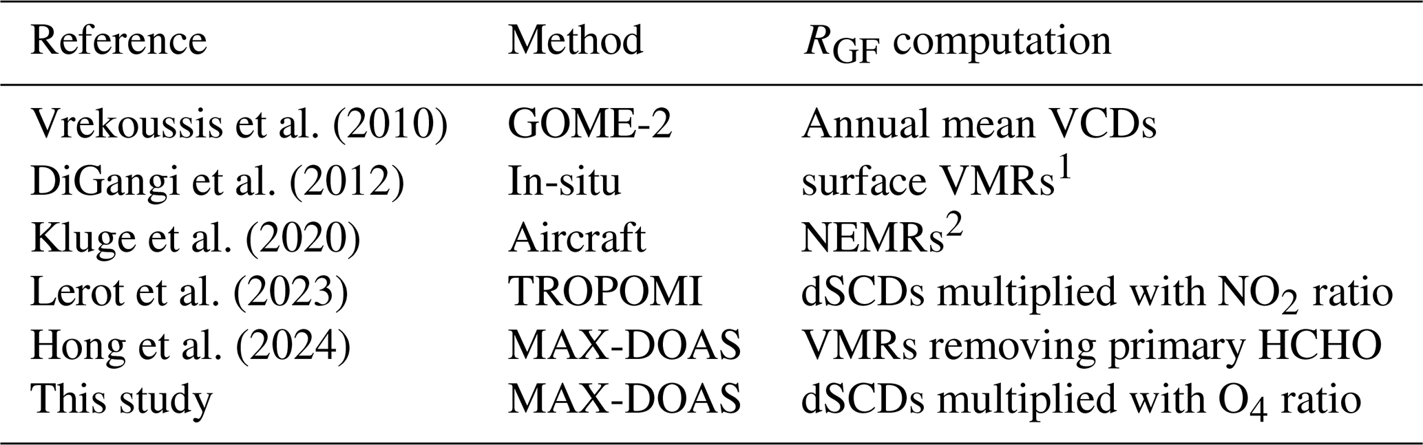
1 Volume mixing ratio.
2 Normalised excess mixing ratio.
Firstly, VMRs obtained by in-situ measurements determine the RGF at the position of the instrument at the sampling time. Here RGF represents the smallest measurement volume, a point measurement. For RGF values computed via dSCDs from a low elevation angle with O4 correction (this work), the situation is similar to RGF via VMRs. However, a different volume is probed. Looking towards the horizon, the retrieved dSCDs are dominated by absorption in the lowest layer. Therefore, the resulting RGF is dominated by the volume along the average light path close to the surface until the scattering point. Lastly, there is column-averaged RGF from either ground-based instruments or satellite-based instruments. Both platforms allow to probe the whole atmospheric column, however with different vertical sensitivities, see Sect. 3.4.2. The column-averaged RGF represents the whole column including the vertical information about the trace gases. However, satellite columns are obtained for the whole ground pixel area, which is larger than the inherent spatial averaging for ground-based columns due to the field of view (FOV).
So even though, all ratios of CHOCHO and HCHO are called RGF, they do not necessarily represent the same measurement volume. Different measurement volumes go along with different kinds of averaging or no averaging at all in the case of in-situ RGF. Therefore, processes of different scales (spatial or temporal) contribute differently to the RGF representing different measurement volumes.
3.4.2 Vertical sensitivity
As discussed in the validation study of the TROPOMI HCHO product using ground-based MAX-DOAS observations by De Smedt et al. (2021), satellites and ground-based MAX-DOAS instruments have opposite vertical sensitivity profiles. Satellite-based instruments have minimal sensitivity near the surface, whereas MAX-DOAS instruments are most sensitive at the surface, with sensitivity decreasing to near zero above approximately 3 km altitude. De Smedt et al. (2021) found that accounting for these sensitivity differences can reduce the bias between the two platforms by up to 20 %.
For RGF, this implies that satellite-derived values are biased toward higher atmospheric layers compared to ground-based measurements, even when vertical profiles or vertical column densities (VCDs) are used. Notably, previous studies have shown that RGF can vary with altitude. For example, Xing et al. (2020) demonstrated that the diurnal behaviour of RGF changes significantly within the lowest 1 km, which may help explain some discrepancies between satellite and ground-based observations.
3.4.3 Temporal sampling
Pronounced diurnal and seasonal cycles in are visible at anthropogenic sites in our dataset. In the presence of such cycles, the time/period of measurement becomes critical. For short duration campaigns, the seasonal cycle has to be considered to avoid a sampling bias.
The diurnal cycle plays an important role when intercomparing satellites or comparing satellites with ground-based instruments. Sun-synchronous low-Earth orbit satellites, such as the one hosting the TROPOMI instrument, pass at a fixed local solar time over the equator and thus only capture a snapshot of the diurnal variability. Given that our observed diurnal cycles are relatively symmetric around noon and the overpass times surround noon (see Fig. 5), only minor differences are expected between commonly used satellite instruments such as GOME-2, SCIAMACHY, TROPOMI, and OMI. Only for Athens, the diurnal cycle is shifted to earlier hours, so a notable effect is observed: the measurements during morning overpass are higher by approximately 0.5 %pt. than the afternoon.
When comparing satellite measurements to ground-based instruments, however, systematic differences can emerge in daily averages. In the most extreme case, for Incheon, this could result in an overestimation by TROPOMI of about 0.5 %pt. relative to the daily average. Importantly, since diurnal variability is most pronounced at anthropogenic sites, the magnitude of this effect differs across environments. Consequently, a spatially variable bias is expected between studies relying solely on satellite data and those based on ground-based observations. When directly comparing both platforms, it is important to use only data close to the overpass time to eliminate this bias. It is worth noting that new and upcoming geostationary satellites (e.g., GEMS, TEMPO, Sentinel-4) provide diurnal coverage, which should help eliminate such biases when comparing RGF from different platforms.
3.4.4 Impact of averaging-ratioing order
In the literature, one can find two different methodologies to computation RGF values. Firstly, RGF as the mean of the individual ratios (in the following called instantaneous RGF) and, secondly, RGF as the ratio of the mean of the HCHO and CHOCHO columns (in the following called global RGF).
Both approaches can be applied to any aggregated dataset, but in practise the global ratio is often used for RGF based on satellite data. Satellite retrievals are more challenging than ground-based retrievals: the increased distance to surface-level trace gases and the satellite viewing geometry result in lower sensitivity near the surface (Lerot et al., 2021) and the short integration time limits the signal to noise ratio of the individual measurement. To improve the signal-to-noise ratio, satellite measurements are commonly averaged over a defined period and area (Lerot et al., 2021) before calculating RGF from the averaged VCDs. The instantaneous RGF is primarily applied for datasets from ground-based instruments, as in this work, since the ground-based instruments generally provide a higher signal-to-noise ratio due to a longer integration time.
The order of operations matters as the division and the mean do not commute in general , so the ratio of means (global RGF, Eq. 9) is not the mean of ratios (instantaneous RGF, Eq. 8). Here N refers to the number of CHOCHO dSCDs and M refers to the number of HCHO dSCDs. The instantaneous RGF requires pairs of simultaneous CHOCHO and HCHO measurements (M = N), therefore ensuring direct comparability but reducing data coverage. The global RGF is more forgiving and allows filtering every trace gas individually (M ≠ N), leading to potential sampling biases. If valid CHOCHO data occur mainly in summer while valid HCHO measurements are available throughout the whole year, the resulting global RGF would mix a seasonal average with an annual average and thus misrepresent the true annual relationship of CHOCHO and HCHO.
As the usage of the global RGF is required for practical reasons, we investigate how both approaches differ by applying both methodologies to our ground-based dataset. The quality filters are applied in a way, consistent with the previous sections, that only valid pairs of simultaneous CHOCHO and HCHO measurements (M = N) are considered for the analysis.
The instantaneous RGF consistently yields higher values compared to the global RGF across all analyses made during this study. A clear systematic bias is visible for the differences between the instantaneous RGF and the global RGF in Fig. 13, and the magnitude of this bias varies depending on the station, month, and time of day. Looking at the diurnal cycles, a large systematic difference is present at ATTO (Fig. 13a) throughout the day. The largest differences occur in Orléans (Fig. 13b), where discrepancies reach just below 1 %pt. around 10:00 LST. In contrast, the anthropogenic sites Incheon and Athens (Fig. 13c, d) show much closer agreement between the two approaches, with overall smaller differences. A more detailed view of the 10:00 LST bin distributions, as well as extended daily time series for Orléans, is provided in the Supplement (Figs. S5 and S6).
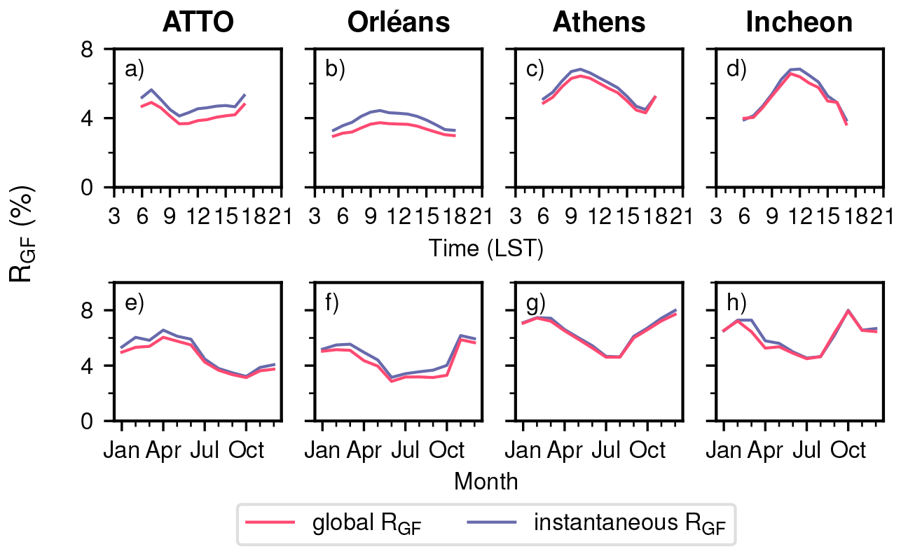
Figure 13Diurnal cycles (top row) and seasonal cycles (bottom row) of RGF (without O4 correction) for all four sites.
The magnitude of the difference between both methods depends primarily on the variability and shape of the underlying HCHO and CHOCHO distributions within each bin, as well as on their correlation. The consistently higher instantaneous RGF values are driven by small HCHO dSCDs in the denominator, which disproportionately increase individual ratios and introduce skewness. Consequently, the bias between both methods increases with growing asymmetry of the ratio distribution. For a more formal reasoning of the conditions under which the ratio of means equals the mean of ratios see Heijmans (1999).
Over the past decade, the literature has reported multiple inconclusive findings regarding the ratio of glyoxal-to-formaldehyde, RGF, and its use as a proxy for VOC source identification. In this study, we use a multi-year ground-based MAX-DOAS dataset at four stations to revisit RGF and reassess its drivers and limitations. Our dataset includes four MAX-DOAS stations located in different environments, allowing us to systematically investigate patterns in the data. Additionally, we compare the results with various meteorological variables and other trace gases.
We find differences in the absolute magnitudes of across environments: lower values at the biogenic sites (ATTO and Orléans) and high values at the strongly anthropogenic sites (Incheon and Athens). While the dSCDs of CHOCHO and HCHO are similarly high across all stations, both trace gases show different behaviours. Glyoxal is notably enhanced at the anthropogenic sites and serves as the primary factor driving the differences in absolute magnitudes. This offset is consistently observed in the seasonal, weekly, and diurnal cycles.
In addition, we observe a seasonal cycle characterised by higher values during the Northern Hemisphere winter months and lower values during the summer months, primarily driven by the pronounced seasonal cycle of HCHO, which is strongly linked to temperature. This pattern holds across all stations except ATTO, where the seasonal cycle is shifted by several months and exhibits enhanced values during the wet and reduced values during the dry season (Donner, 2024).
The diurnal cycles of are relatively flat at the biogenic stations but pronounced at the anthropogenic stations, showing variations of approximately 2 %pt. with peaks occurring before or around noon. Glyoxal, in particular, exhibits a distinct diurnal pattern at the anthropogenic sites compared to the biogenic sites, making it the main driver of the observed diurnal variability. We also detect a weak weekend effect at the anthropogenic stations, with decreasing by about 10 % compared to weekdays, primarily due to a stronger reduction by CHOCHO on the weekend.
Moreover, we investigated the link to meteorology of . It exhibits a clear temperature dependence. Above approximately 15 °C, HCHO levels increase more strongly with temperature than CHOCHO, leading to a hyperbolic decrease in beyond this temperature. Accounting for the temperature dependence with a regression-based approach removes all variation of with other meteorological variables due to their intercorrelation. The seasonal cycle of for non-tropical sites is removed, whereas the diurnal cycle remains.
Our investigation of the dependence of the RGF–NO2 relationship implies that cannot be linked only to different NO2 levels. Local effects and VOC emission characteristics may play a more significant role than previously assumed. Thus site-specific considerations for the usage of as a proxy for VOC type might be required. Overall, both the diurnal cycles and the relationship to NO2 suggest that CHOCHO is more closely associated with anthropogenic activity than HCHO.
Finally, we examine four factors that can impact comparisons of RGF from different datasets. Firstly, RGF, computed from different measurement techniques, inherently average over different measurement volumes. In addition, the vertical sensitivity of satellites and ground-based instruments is not identical. Moreover, due to the pronounced seasonal and diurnal cycles, the time of the measurement becomes critical. No significant difference between different overpass times of GOME-2, SCIAMACHY, and TROPOMI/OMI is observed due to the symmetric diurnal cycles; however the overpass time has to be considered for ground-based and satellite comparisons. Lastly, we investigate the impact of the order of ratioing and averaging. The global RGF is generally biased low compared to the instantaneous RGF as no extreme values occur in the denominator.
Future work should quantify these effects through radiative transfer simulations or direct instrument intercomparisons. Beyond this, expanding the network of long-term ground-based observations would strengthen the statistical basis and broaden the range of environments and source regimes captured, ultimately advancing the interpretation of RGF as a proxy for VOC origin. Improved coverage of simultaneous VOC precursor measurements would further enhance the interpretation of observational data. An important complementary perspective could come from modeling studies. In particular, sensitivity studies using chemical box models (including multiphase chemistry) offer a unique opportunity to challenge current understanding. By systematically turning individual processes on or off, such models can help disentangle complex interconnections that are difficult to isolate in observational data. Additionally, distinguishing between the primary and secondary formation of HCHO and CHOCHO in the context of RGF could help clarify the underlying mechanisms (Hong et al., 2024; Xing et al., 2025).
Given these complexities, using the glyoxal-to-formaldehyde ratio as a proxy for VOC source identification remains challenging. While we observe clear differences in the absolute magnitudes of across stations in different environments, suggesting that the ratio carries valuable environmental information, our incomplete understanding of emissions, VOC precursors, and the detailed chemistry of HCHO and CHOCHO currently limits the reliable use of as a robust proxy for VOC source attribution.
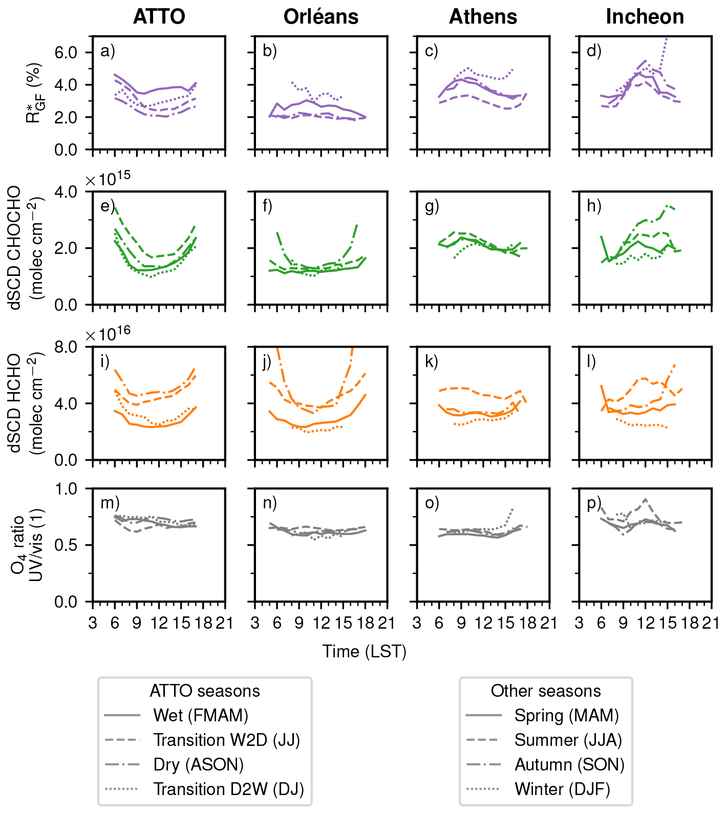
Figure A1Diurnal cycles of (top row), CHOCHO dSCD (upper centre row), HCHO dSCD (lower centre row), and O4 ratio (bottom row) filtered by season for ATTO, Orléans, Athens, and Incheon relative to local solar time (LST). Note that the months for ATTO are grouped differently to account for wet and dry season. Panels (e) and (i) are self-created based on Donner (2024).
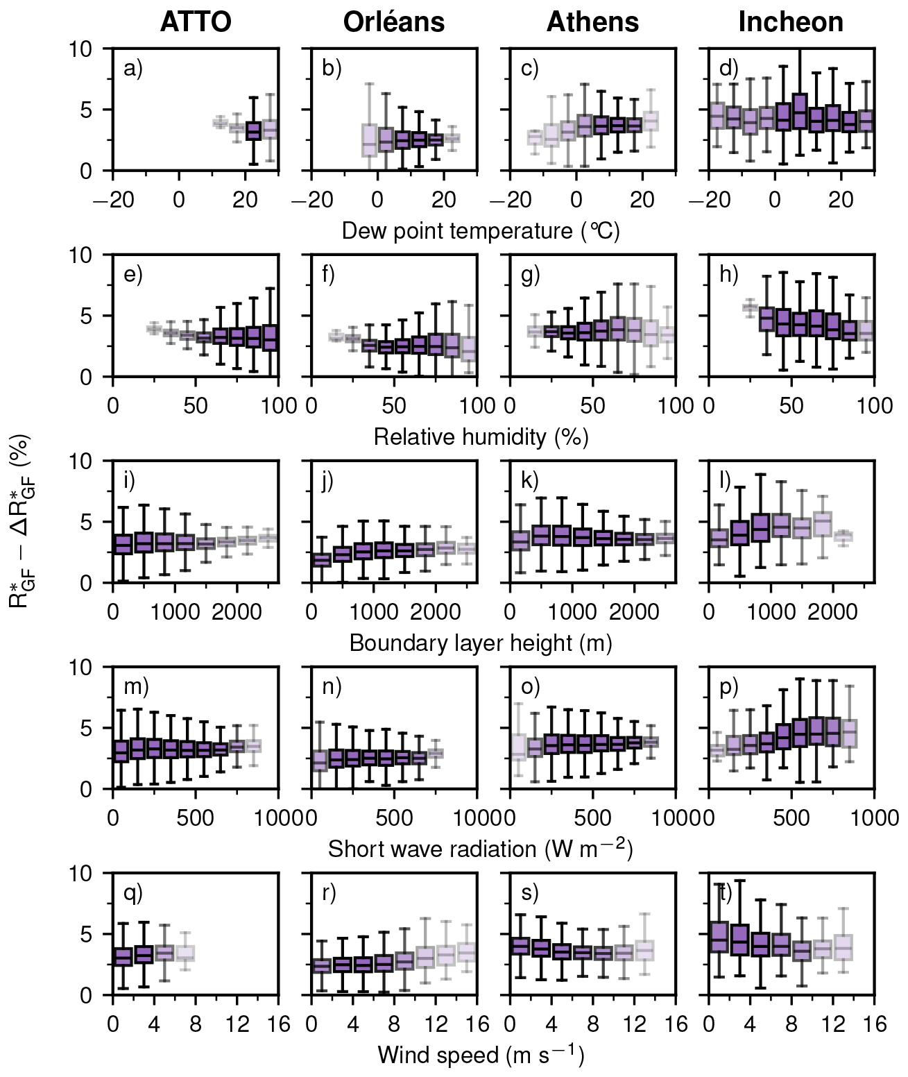
Figure A2Temperature-normalised as a function of binned meteorological variables from ERA5. Within each box, the horizontal line indicates the median and the box spans the IQR; whiskers extend to 1.5 IQR. Box transparency scales with the number of contributing measurements, with more transparent boxes indicating fewer observations. Missing box plots indicate that no data points fall within that interval.
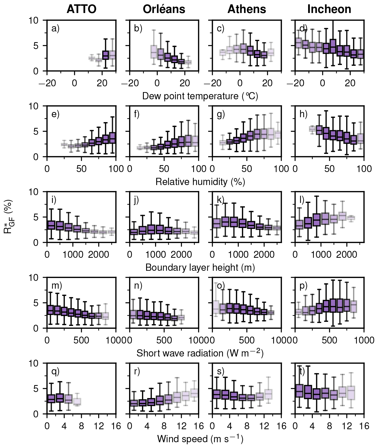
Figure A3 as a function of binned meteorological variables from ERA5. Within each box, the horizontal line indicates the median and the box spans the IQR; whiskers extend to 1.5 IQR. Box transparency scales with the number of contributing measurements, with more transparent boxes indicating fewer observations. Missing box plots indicate that no data points fall within that interval.
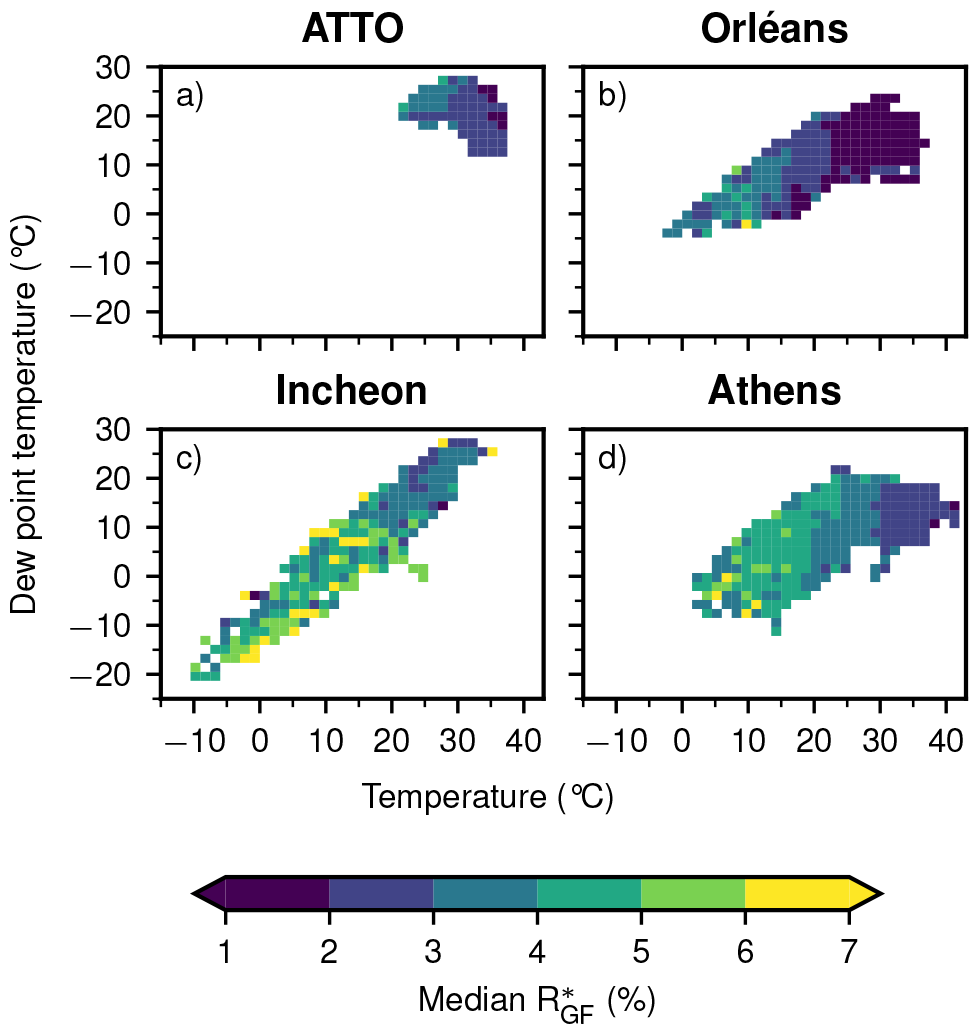
The ERA5 atmospheric reanalysis data were downloaded from the from the Copernicus Climate Change (C3S) climate data store (CDS): https://doi.org/10.24381/cds.adbb2d47 (Hersbach et al., 2023). The emission datasets, CAMS-GLOB-ANT version 6.2 and CAMS-GLOB-BIO version 3.1, were downloaded from ECCAD: https://permalink.aeris-data.fr/CAMS-GLOB-ANT (last access: 8 January 2026; Granier et al., 2019). MAX-DOAS data are available from the authors on request.
The supplement related to this article is available online at https://doi.org/10.5194/acp-26-8809-2026-supplement.
SB, AR, and MV contributed to the conceptualization, methodology, data interpretation and writing of the original draft. SB and BZ set-up and operated the instrument in Orléans. SD and TW conducted the measurements and provided the ATTO data set. APP performed the backwards sensitivity studies. LA provided expertise regarding the fit settings for the Bremen instruments. SB processed the data and performed the data analysis. All authors have contributed with scientific discussions to data interpretation.
At least one of the (co-)authors is a member of the editorial board of Atmospheric Chemistry and Physics. The peer-review process was guided by an independent editor, and the authors also have no other competing interests to declare.
The results contain modified Copernicus Climate Change Service information 2020. Neither the European Commission nor ECMWF is responsible for any use that may be made of the Copernicus information or data it contains.
Publisher's note: Copernicus Publications remains neutral with regard to jurisdictional claims made in the text, published maps, institutional affiliations, or any other geographical representation in this paper. The authors bear the ultimate responsibility for providing appropriate place names. Views expressed in the text are those of the authors and do not necessarily reflect the views of the publisher.
AI Usage: Reformatting tables, improving code for figures, indexing literature, improved text readability, and spelling correction. Simulations were performed on the HPC cluster Aether at the University of Bremen. The authors thank Morgan Lopez, Dylan Lopez, and Christof Petri for their support in maintaining the Traînou (Orléans) measurement site. The ATTO site is operated and managed by INPA and MPG. The authors also acknowledge the whole ATTO team for maintenance and operation of the ATTO site and its infrastructure. Further, Bianca Lauster and Steffen Ziegler are acknowledged for their large contribution in operating and maintaining the ATTO MAX-DOAS instrument. The authors thank Myrto Gratsea and NOA for supporting the station in Athens and the GMAP and SIJAQ teams for facilitating measurements in Incheon. This work was supported by the Data Science Center of the University of Bremen (DSC@UB) funded by the State of Bremen.
The ATTO research has been supported by the German Federal Ministry of Education and Research (BMBF contract no. 01LK2101B). Measurements in Incheon have received funding from NIER. SB, MV, AR have been supported by the University of Bremen. SB has been supported by the Erasmus+ (grant no. 101056066). MV, APP and the HPC cluster Aether have been supported by the Deutsche Forschungsgemeinschaft (DFG, German Research Foundation) under Germany's Excellence Strategy (University Allowance, EXC 2077, University of Bremen). MV and APP have been supported by the EARTHONE HORIZON Research and Innovation project (grant no. 101181825).
The article processing charges for this open-access publication were covered by the University of Bremen.
This paper was edited by Chiara Giorio and reviewed by Yang Xiao, Zijun Li, and three anonymous referees.
Alvarado, L. M. A., Richter, A., Vrekoussis, M., Hilboll, A., Kalisz Hedegaard, A. B., Schneising, O., and Burrows, J. P.: Unexpected long-range transport of glyoxal and formaldehyde observed from the Copernicus Sentinel-5 Precursor satellite during the 2018 Canadian wildfires, Atmos. Chem. Phys., 20, 2057–2072, https://doi.org/10.5194/acp-20-2057-2020, 2020. a
Andreae, M. O. and Merlet, P.: Emission of trace gases and aerosols from biomass burning, Global Biogeochem. Cy., 15, 955–966, https://doi.org/10.1029/2000gb001382, 2001. a
Andreae, M. O., Acevedo, O. C., Araùjo, A., Artaxo, P., Barbosa, C. G. G., Barbosa, H. M. J., Brito, J., Carbone, S., Chi, X., Cintra, B. B. L., da Silva, N. F., Dias, N. L., Dias-Júnior, C. Q., Ditas, F., Ditz, R., Godoi, A. F. L., Godoi, R. H. M., Heimann, M., Hoffmann, T., Kesselmeier, J., Könemann, T., Krüger, M. L., Lavric, J. V., Manzi, A. O., Lopes, A. P., Martins, D. L., Mikhailov, E. F., Moran-Zuloaga, D., Nelson, B. W., Nölscher, A. C., Santos Nogueira, D., Piedade, M. T. F., Pöhlker, C., Pöschl, U., Quesada, C. A., Rizzo, L. V., Ro, C.-U., Ruckteschler, N., Sá, L. D. A., de Oliveira Sá, M., Sales, C. B., dos Santos, R. M. N., Saturno, J., Schöngart, J., Sörgel, M., de Souza, C. M., de Souza, R. A. F., Su, H., Targhetta, N., Tóta, J., Trebs, I., Trumbore, S., van Eijck, A., Walter, D., Wang, Z., Weber, B., Williams, J., Winderlich, J., Wittmann, F., Wolff, S., and Yáñez-Serrano, A. M.: The Amazon Tall Tower Observatory (ATTO): overview of pilot measurements on ecosystem ecology, meteorology, trace gases, and aerosols, Atmos. Chem. Phys., 15, 10723–10776, https://doi.org/10.5194/acp-15-10723-2015, 2015. a
Beirle, S., Platt, U., Wenig, M., and Wagner, T.: Weekly cycle of NO2 by GOME measurements: a signature of anthropogenic sources, Atmos. Chem. Phys., 3, 2225–2232, https://doi.org/10.5194/acp-3-2225-2003, 2003. a
Bell, M. L., McDermott, A., Zeger, S. L., Samet, J. M., and Dominici, F.: Ozone and Short-term Mortality in 95 US Urban Communities, 1987-2000, JAMA, 292, 2372–2378, https://doi.org/10.1001/jama.292.19.2372, 2004. a
Bello, J., Vallet, P., Perot, T., Balandier, P., Seigner, V., Perret, S., Couteau, C., and Korboulewsky, N.: How do mixing tree species and stand density affect seasonal radial growth during drought events?, Forest Ecol. Manag., 432, 436–445, https://doi.org/10.1016/j.foreco.2018.09.044, 2019. a
Berg, F., Novelli, A., Dubus, R., Hofzumahaus, A., Holland, F., Wahner, A., and Fuchs, H.: Temperature-dependent rate coefficients for the reactions of OH radicals with selected alkanes, aromatic compounds, and monoterpenes, Atmos. Chem. Phys., 24, 13715–13731, https://doi.org/10.5194/acp-24-13715-2024, 2024. a
Bourtsoukidis, E., Pozzer, A., Williams, J., Makowski, D., Peñuelas, J., Matthaios, V. N., Lazoglou, G., Yañez-Serrano, A. M., Lelieveld, J., Ciais, P., Vrekoussis, M., Daskalakis, N., and Sciare, J.: High temperature sensitivity of monoterpene emissions from global vegetation, Communications Earth & Environment, 5, https://doi.org/10.1038/s43247-023-01175-9, 2024. a, b
Castro-Melgar, I., Tsagkou, A., Zacharopoulou, M., Basiou, E., Athinelis, I., Katris, E.-A., Kalavrezou, I.-E., and Parcharidis, I.: Wildfires During Early Summer in Greece (2024): Burn Severity and Land Use Dynamics Through Sentinel-2 Data, Forests, 16, 268, https://doi.org/10.3390/f16020268, 2025. a
Chen, Y., Liu, C., Su, W., Hu, Q., Zhang, C., Liu, H., and Yin, H.: Identification of volatile organic compound emissions from anthropogenic and biogenic sources based on satellite observation of formaldehyde and glyoxal, Sci. Total Environ., 859, 159997, https://doi.org/10.1016/j.scitotenv.2022.159997, 2023. a, b, c, d
Chan Miller, C., Gonzalez Abad, G., Wang, H., Liu, X., Kurosu, T., Jacob, D. J., and Chance, K.: Glyoxal retrieval from the Ozone Monitoring Instrument, Atmos. Meas. Tech., 7, 3891–3907, https://doi.org/10.5194/amt-7-3891-2014, 2014. a, b
Chan Miller, C., Jacob, D. J., González Abad, G., and Chance, K.: Hotspot of glyoxal over the Pearl River delta seen from the OMI satellite instrument: implications for emissions of aromatic hydrocarbons, Atmos. Chem. Phys., 16, 4631–4639, https://doi.org/10.5194/acp-16-4631-2016, 2016. a, b, c
Chan Miller, C., Jacob, D. J., Marais, E. A., Yu, K., Travis, K. R., Kim, P. S., Fisher, J. A., Zhu, L., Wolfe, G. M., Hanisco, T. F., Keutsch, F. N., Kaiser, J., Min, K.-E., Brown, S. S., Washenfelder, R. A., González Abad, G., and Chance, K.: Glyoxal yield from isoprene oxidation and relation to formaldehyde: chemical mechanism, constraints from SENEX aircraft observations, and interpretation of OMI satellite data, Atmos. Chem. Phys., 17, 8725–8738, https://doi.org/10.5194/acp-17-8725-2017, 2017. a
Crameri, F., Shephard, G. E., and Heron, P. J.: The misuse of colour in science communication, Nat. Commun., 11, https://doi.org/10.1038/s41467-020-19160-7, 2020. a
Delacre, M., Lakens, D., and Leys, C.: Why Psychologists Should by Default Use Welch's t-test Instead of Student's t-test, International Review of Social Psychology, 30, 92–101, https://doi.org/10.5334/irsp.82, 2017. a
Delacre, M., Leys, C., Mora, Y. L., and Lakens, D.: Taking Parametric Assumptions Seriously: Arguments for the Use of Welch’s F-test instead of the Classical F-test in One-Way ANOVA, International Review of Social Psychology, 32, 13, https://doi.org/10.5334/irsp.198, 2019. a
Derwent, R. G., Jenkin, M. E., Utembe, S. R., Shallcross, D. E., Murrells, T. P., and Passant, N. R.: Secondary organic aerosol formation from a large number of reactive man-made organic compounds, Sci. Total Environ., 408, 3374–3381, https://doi.org/10.1016/j.scitotenv.2010.04.013, 2010. a
De Smedt, I., Pinardi, G., Vigouroux, C., Compernolle, S., Bais, A., Benavent, N., Boersma, F., Chan, K.-L., Donner, S., Eichmann, K.-U., Hedelt, P., Hendrick, F., Irie, H., Kumar, V., Lambert, J.-C., Langerock, B., Lerot, C., Liu, C., Loyola, D., Piters, A., Richter, A., Rivera Cárdenas, C., Romahn, F., Ryan, R. G., Sinha, V., Theys, N., Vlietinck, J., Wagner, T., Wang, T., Yu, H., and Van Roozendael, M.: Comparative assessment of TROPOMI and OMI formaldehyde observations and validation against MAX-DOAS network column measurements, Atmos. Chem. Phys., 21, 12561–12593, https://doi.org/10.5194/acp-21-12561-2021, 2021. a, b
Dienhart, D., Crowley, J. N., Bourtsoukidis, E., Edtbauer, A., Eger, P. G., Ernle, L., Harder, H., Hottmann, B., Martinez, M., Parchatka, U., Paris, J.-D., Pfannerstill, E. Y., Rohloff, R., Schuladen, J., Stönner, C., Tadic, I., Tauer, S., Wang, N., Williams, J., Lelieveld, J., and Fischer, H.: Measurement report: Observation-based formaldehyde production rates and their relation to OH reactivity around the Arabian Peninsula, Atmos. Chem. Phys., 21, 17373–17388, https://doi.org/10.5194/acp-21-17373-2021, 2021. a
DiGangi, J. P., Henry, S. B., Kammrath, A., Boyle, E. S., Kaser, L., Schnitzhofer, R., Graus, M., Turnipseed, A., Park, J.-H., Weber, R. J., Hornbrook, R. S., Cantrell, C. A., Maudlin III, R. L., Kim, S., Nakashima, Y., Wolfe, G. M., Kajii, Y., Apel, E. C., Goldstein, A. H., Guenther, A., Karl, T., Hansel, A., and Keutsch, F. N.: Observations of glyoxal and formaldehyde as metrics for the anthropogenic impact on rural photochemistry, Atmos. Chem. Phys., 12, 9529–9543, https://doi.org/10.5194/acp-12-9529-2012, 2012. a, b, c, d, e, f, g, h, i
Donner, S.: Retrieving vertical profiles and tropospheric columns of formaldehyde from global long-term MAX-DOAS measurements, PhD thesis, Johannes Gutenberg-Universität Mainz, https://doi.org/10.25358/OPENSCIENCE-11085, 2024. a, b, c, d, e, f, g, h, i, j, k, l, m, n
Ehhalt, D., Prather, M., Dentener, F., Derwent, R., Dlugokencky, E., Holland, E., Isaksen, I., Katima, J., Kirchhoff, V., Matson, P., Midgley, P., and Wang, M.: Atmospheric Chemistry and Greenhouse Gases. In: Climate Change 2001: The Scientific Basis. Contribution of Working Group I to the Third Assessment Report of the Intergovernmental Panel on Climate Change, edited by: Houghton, J. T., Ding, Y., Griggs, D. J., Noguer, M., van der Linden, P. J., Dai, X., Maskell, K., Johnson, C. A., Cambridge University Press, ISBN 0521807670, 2001. a
European Environment Agency: Harm to human health from air pollution in Europe: burden of disease status, Briefing no. 21/2024, https://doi.org/10.2800/3950756, 2024. a
Finkenzeller, H. and Volkamer, R.: O2–O2 CIA in the gas phase: Cross-section of weak bands, and continuum absorption between 297–500 nm, J. Quant. Spectrosc. Ra., 279, 108063, https://doi.org/10.1016/j.jqsrt.2021.108063, 2022. a
Fortems-Cheiney, A., Chevallier, F., Pison, I., Bousquet, P., Saunois, M., Szopa, S., Cressot, C., Kurosu, T. P., Chance, K., and Fried, A.: The formaldehyde budget as seen by a global-scale multi-constraint and multi-species inversion system, Atmos. Chem. Phys., 12, 6699–6721, https://doi.org/10.5194/acp-12-6699-2012, 2012. a
Franco, B., Marais, E. A., Bovy, B., Bader, W., Lejeune, B., Roland, G., Servais, C., and Mahieu, E.: Diurnal cycle and multi-decadal trend of formaldehyde in the remote atmosphere near 46° N, Atmos. Chem. Phys., 16, 4171–4189, https://doi.org/10.5194/acp-16-4171-2016, 2016. a
Fu, T.-M., Jacob, D. J., Wittrock, F., Burrows, J. P., Vrekoussis, M., and Henze, D. K.: Global budgets of atmospheric glyoxal and methylglyoxal, and implications for formation of secondary organic aerosols, J. Geophys. Res.-Atmos., 113, https://doi.org/10.1029/2007JD009505, 2008. a, b, c, d, e
Games, P. A. and Howell, J. F.: Pairwise Multiple Comparison Procedures with Unequal N's and/or Variances: A Monte Carlo Study, J. Educ. Stat., 1, 113–125, https://doi.org/10.3102/10769986001002113, 1976. a
Gilman, J. B., Lerner, B. M., Kuster, W. C., Goldan, P. D., Warneke, C., Veres, P. R., Roberts, J. M., de Gouw, J. A., Burling, I. R., and Yokelson, R. J.: Biomass burning emissions and potential air quality impacts of volatile organic compounds and other trace gases from fuels common in the US, Atmos. Chem. Phys., 15, 13915–13938, https://doi.org/10.5194/acp-15-13915-2015, 2015. a
Goldstein, A. H. and Galbally, I. E.: Known and Unexplored Organic Constituents in the Earth’s Atmosphere, Environ. Sci. Technol., 41, 1514–1521, https://doi.org/10.1021/es072476p, 2007. a
Granier, C., Darras, S., Denier van der Gon, H., Doubalova, J., Elguindi, N., Galle, B., Gauss, M., Guevara, M., Jalkanen, J.-P., Kuenen, J., Liousse, C., Quack, B., Simpson, D., and Sindelarova, K.: The Copernicus Atmosphere Monitoring Service global and regional emissions (April 2019 version), Copernicus Atmosphere Monitoring Service (CAMS), https://doi.org/10.24380/D0BN-KX16, 2019. a, b
Gratsea, M., Vrekoussis, M., Richter, A., Wittrock, F., Schönhardt, A., Burrows, J., Kazadzis, S., Mihalopoulos, N., and Gerasopoulos, E.: Slant column MAX-DOAS measurements of nitrogen dioxide, formaldehyde, glyoxal and oxygen dimer in the urban environment of Athens, Atmos. Environ., 135, 118–131, https://doi.org/10.1016/j.atmosenv.2016.03.048, 2016. a, b, c, d
Guenther, A., Hewitt, C. N., Erickson, D., Fall, R., Geron, C., Graedel, T., Harley, P., Klinger, L., Lerdau, M., Mckay, W. A., Pierce, T., Scholes, B., Steinbrecher, R., Tallamraju, R., Taylor, J., and Zimmerman, P.: A global model of natural volatile organic compound emissions, J. Geophys. Res.-Atmos., 100, 8873–8892, https://doi.org/10.1029/94jd02950, 1995. a
Guenther, A. B., Zimmerman, P. R., Harley, P. C., Monson, R. K., and Fall, R.: Isoprene and monoterpene emission rate variability: Model evaluations and sensitivity analyses, J. Geophys. Res.-Atmos., 98, 12609–12617, https://doi.org/10.1029/93jd00527, 1993. a
Guenther, A. B., Jiang, X., Heald, C. L., Sakulyanontvittaya, T., Duhl, T., Emmons, L. K., and Wang, X.: The Model of Emissions of Gases and Aerosols from Nature version 2.1 (MEGAN2.1): an extended and updated framework for modeling biogenic emissions, Geosci. Model Dev., 5, 1471–1492, https://doi.org/10.5194/gmd-5-1471-2012, 2012. a
Guo, Y., Wang, S., Zhu, J., Zhang, R., Gao, S., Saiz-Lopez, A., and Zhou, B.: Atmospheric formaldehyde, glyoxal and their relations to ozone pollution under low- and high-NOx regimes in summertime Shanghai, China, Atmos. Res., 258, 105635, https://doi.org/10.1016/j.atmosres.2021.105635, 2021. a
Haagen-Smit, A. J.: Chemistry and Physiology of Los Angeles Smog, Industrial & Engineering Chemistry, 44, 1342–1346, https://doi.org/10.1021/ie50510a045, 1952. a
Hallquist, M., Wenger, J. C., Baltensperger, U., Rudich, Y., Simpson, D., Claeys, M., Dommen, J., Donahue, N. M., George, C., Goldstein, A. H., Hamilton, J. F., Herrmann, H., Hoffmann, T., Iinuma, Y., Jang, M., Jenkin, M. E., Jimenez, J. L., Kiendler-Scharr, A., Maenhaut, W., McFiggans, G., Mentel, Th. F., Monod, A., Prévôt, A. S. H., Seinfeld, J. H., Surratt, J. D., Szmigielski, R., and Wildt, J.: The formation, properties and impact of secondary organic aerosol: current and emerging issues, Atmos. Chem. Phys., 9, 5155–5236, https://doi.org/10.5194/acp-9-5155-2009, 2009. a
Heijmans, R.: When does the expectation of a ratio equal the ratio of expectations?, Stat. Pap., 40, 107–115, https://doi.org/10.1007/bf02927114, 1999. a
Hellenic Statistical Authority: Attiki census results of population and housing – ELSTAT 2021, https://www.statistics.gr/documents/20181/18409455/population_ATTICA_EN.pdf/f8156495-873d-bb66-bf8e-b87bf6974e14 (last access: 10 March 2026), 2024. a, b
Hersbach, H., Bell, B., Berrisford, P., Biavati, G., Horányi, A., Muñoz Sabater, J., Nicolas, J., Peubey, C., Radu, R., Rozum, I., Schepers, D., Simmons, A., Soci, C., Dee, D., and Thépaut, J.-N.: ERA5 hourly data on single levels from 1940 to present, Copernicus Climate Change Service (C3S) Climate Data Store (CDS) [data set], https://doi.org/10.24381/cds.adbb2d47, 2023. a, b
Hong, Q., Xing, J., Xing, C., Yang, B., Su, W., Chen, Y., Zhang, C., Zhu, Y., and Liu, C.: Investigating vertical distributions and photochemical indications of formaldehyde, glyoxal, and NO2 from MAX-DOAS observations in four typical cities of China, Sci. Total Environ., 954, 176447, https://doi.org/10.1016/j.scitotenv.2024.176447, 2024. a, b, c, d
Hoque, H. M. S., Irie, H., and Damiani, A.: First MAX-DOAS Observations of Formaldehyde and Glyoxal in Phimai, Thailand, J. Geophys. Res.-Atmos., 123, 9957–9975, https://doi.org/10.1029/2018jd028480, 2018a. a, b, c, d, e, f, g, h, i
Hoque, H. M. S., Irie, H., Damiani, A., Rawat, P., and Naja, M.: First Simultaneous Observations of Formaldehyde and Glyoxal by MAX-DOAS in the Indo-Gangetic Plain Region, SOLA, 14, 159–164, https://doi.org/10.2151/sola.2018-028, 2018b. a, b, c, d, e, f
Hönninger, G., von Friedeburg, C., and Platt, U.: Multi axis differential optical absorption spectroscopy (MAX-DOAS), Atmos. Chem. Phys., 4, 231–254, https://doi.org/10.5194/acp-4-231-2004, 2004. a, b
Institut national de la statistique et des études économiques: Populations de référence 2022 – Commune d'Orléans (45234), https://www.insee.fr/fr/statistiques/8288323?geo=COM-45234 (last access: 10 March 2026), 2024. a
Institut national de la statistique et des études économiques: Dossier complet – Commune de Traînou (45327), https://www.insee.fr/fr/statistiques/2011101?geo=COM-45327 (last access: 10 March 2026), 2025. a
Instituto Brasileiro de Geografia e Estatística: Panorama Censo 2022 – Manaus, https://censo2022.ibge.gov.br/panorama/ (last access: 10 March 2026), 2022. a
Irie, H., Takashima, H., Kanaya, Y., Boersma, K. F., Gast, L., Wittrock, F., Brunner, D., Zhou, Y., and Van Roozendael, M.: Eight-component retrievals from ground-based MAX-DOAS observations, Atmos. Meas. Tech., 4, 1027–1044, https://doi.org/10.5194/amt-4-1027-2011, 2011. a
Kaiser, J., Wolfe, G. M., Min, K. E., Brown, S. S., Miller, C. C., Jacob, D. J., deGouw, J. A., Graus, M., Hanisco, T. F., Holloway, J., Peischl, J., Pollack, I. B., Ryerson, T. B., Warneke, C., Washenfelder, R. A., and Keutsch, F. N.: Reassessing the ratio of glyoxal to formaldehyde as an indicator of hydrocarbon precursor speciation, Atmos. Chem. Phys., 15, 7571–7583, https://doi.org/10.5194/acp-15-7571-2015, 2015. a
Kassomenos, P., Kotroni, V., and Kallos, G.: Analysis of climatological and air quality observations from Greater Athens Area, Atmos. Environ., 29, 3671–3688, https://doi.org/10.1016/1352-2310(94)00358-r, 1995. a
Kim, M.-J., Baek, K.-M., Heo, J.-B., Cheong, J.-P., and Baek, S.-O.: Concentrations, health risks, and sources of hazardous air pollutants in Seoul-Incheon, a megacity area in Korea, Air Qual. Atmos. Hlth., 14, 873–893, https://doi.org/10.1007/s11869-021-00986-z, 2021. a, b
Kluge, F., Hüneke, T., Knecht, M., Lichtenstern, M., Rotermund, M., Schlager, H., Schreiner, B., and Pfeilsticker, K.: Profiling of formaldehyde, glyoxal, methylglyoxal, and CO over the Amazon: normalized excess mixing ratios and related emission factors in biomass burning plumes, Atmos. Chem. Phys., 20, 12363–12389, https://doi.org/10.5194/acp-20-12363-2020, 2020. a
Lagouvardos, K., Kotroni, V., Giannaros, T. M., and Dafis, S.: Meteorological Conditions Conducive to the Rapid Spread of the Deadly Wildfire in Eastern Attica, Greece, B. Am. Meteorol. Soc., 100, 2137–2145, https://doi.org/10.1175/bams-d-18-0231.1, 2019. a
Lange, K., Richter, A., Bösch, T., Zilker, B., Latsch, M., Behrens, L. K., Okafor, C. M., Bösch, H., Burrows, J. P., Merlaud, A., Pinardi, G., Fayt, C., Friedrich, M. M., Dimitropoulou, E., Van Roozendael, M., Ziegler, S., Ripperger-Lukosiunaite, S., Kuhn, L., Lauster, B., Wagner, T., Hong, H., Kim, D., Chang, L.-S., Bae, K., Song, C.-K., Park, J.-U., and Lee, H.: Validation of GEMS tropospheric NO2 columns and their diurnal variation with ground-based DOAS measurements, Atmos. Meas. Tech., 17, 6315–6344, https://doi.org/10.5194/amt-17-6315-2024, 2024. a
Laothawornkitkul, J., Taylor, J. E., Paul, N. D., and Hewitt, C. N.: Biogenic volatile organic compounds in the Earth system, New Phytol., 183, 27–51, https://doi.org/10.1111/j.1469-8137.2009.02859.x, 2009. a
Lee, M., Heikes, B. G., and Jacob, D. J.: Enhancements of hydroperoxides and formaldehyde in biomass burning impacted air and their effect on atmospheric oxidant cycles, J. Geophys. Res.-Atmos., 103, 13201–13212, https://doi.org/10.1029/98jd00578, 1998. a
Lelieveld, J., Evans, J. S., Fnais, M., Giannadaki, D., and Pozzer, A.: The contribution of outdoor air pollution sources to premature mortality on a global scale, Nature, 525, 367–371, https://doi.org/10.1038/nature15371, 2015. a
Lerot, C., Hendrick, F., Van Roozendael, M., Alvarado, L. M. A., Richter, A., De Smedt, I., Theys, N., Vlietinck, J., Yu, H., Van Gent, J., Stavrakou, T., Müller, J.-F., Valks, P., Loyola, D., Irie, H., Kumar, V., Wagner, T., Schreier, S. F., Sinha, V., Wang, T., Wang, P., and Retscher, C.: Glyoxal tropospheric column retrievals from TROPOMI – multi-satellite intercomparison and ground-based validation, Atmos. Meas. Tech., 14, 7775–7807, https://doi.org/10.5194/amt-14-7775-2021, 2021. a, b
Lerot, C., Müller, J.-F., Theys, N., De Smedt, I., Stavrakou, T., and Van Roozendael, M.: Satellite Evidence for Glyoxal Depletion in Elevated Fire Plumes, Geophys. Res. Lett., 50, e2022GL102195, https://doi.org/10.1029/2022GL102195, 2023. a
Li, X., Rohrer, F., Brauers, T., Hofzumahaus, A., Lu, K., Shao, M., Zhang, Y. H., and Wahner, A.: Modeling of HCHO and CHOCHO at a semi-rural site in southern China during the PRIDE-PRD2006 campaign, Atmos. Chem. Phys., 14, 12291–12305, https://doi.org/10.5194/acp-14-12291-2014, 2014. a
Li, X., Zhu, L., De Smedt, I., Sun, W., Chen, Y., Shu, L., Wang, D., Liu, S., Pu, D., Li, J., Zuo, X., Fu, W., Li, Y., Zhang, P., Yan, Z., Fu, T.-M., Shen, H., Wang, C., Ye, J., and Yang, X.: Global Temperature Dependency of Biogenic HCHO Columns Observed From Space: Interpretation of TROPOMI Results Using GEOS-Chem Model, J. Geophys. Res.-Atmos., 129, e2024JD041784, https://doi.org/10.1029/2024JD041784, 2024. a
Liaskoni, M., Huszár, P., Bartík, L., Prieto Perez, A. P., Karlický, J., and Šindelářová, K.: The long-term impact of biogenic volatile organic compound emissions on urban ozone patterns over central Europe: contributions from urban and rural vegetation, Atmos. Chem. Phys., 24, 13541–13569, https://doi.org/10.5194/acp-24-13541-2024, 2024. a
Liu, M. and Matsui, H.: Secondary Organic Aerosol Formation Regulates Cloud Condensation Nuclei in the Global Remote Troposphere, Geophys. Res. Lett., 49, e2022GL100543, https://doi.org/10.1029/2022GL100543, 2022. a
MacDonald, S. M., Oetjen, H., Mahajan, A. S., Whalley, L. K., Edwards, P. M., Heard, D. E., Jones, C. E., and Plane, J. M. C.: DOAS measurements of formaldehyde and glyoxal above a south-east Asian tropical rainforest, Atmos. Chem. Phys., 12, 5949–5962, https://doi.org/10.5194/acp-12-5949-2012, 2012. a
Mavroidis, I. and Ilia, M.: Trends of NOx, NO2 and O3 concentrations at three different types of air quality monitoring stations in Athens, Greece, Atmos. Environ., 63, 135–147, https://doi.org/10.1016/j.atmosenv.2012.09.030, 2012. a
McDuffie, E. E., Smith, S. J., O'Rourke, P., Tibrewal, K., Venkataraman, C., Marais, E. A., Zheng, B., Crippa, M., Brauer, M., and Martin, R. V.: A global anthropogenic emission inventory of atmospheric pollutants from sector- and fuel-specific sources (1970–2017): an application of the Community Emissions Data System (CEDS), Earth Syst. Sci. Data, 12, 3413–3442, https://doi.org/10.5194/essd-12-3413-2020, 2020. a
Myriokefalitakis, S., Vrekoussis, M., Tsigaridis, K., Wittrock, F., Richter, A., Brühl, C., Volkamer, R., Burrows, J. P., and Kanakidou, M.: The influence of natural and anthropogenic secondary sources on the glyoxal global distribution, Atmos. Chem. Phys., 8, 4965–4981, https://doi.org/10.5194/acp-8-4965-2008, 2008. a, b
Nelson, P. F., Tibbett, A. R., and Day, S. J.: Effects of vehicle type and fuel quality on real world toxic emissions from diesel vehicles, Atmos. Environ., 42, 5291–5303, https://doi.org/10.1016/j.atmosenv.2008.02.049, 2008. a
Nguyen, H. T., Kim, K.-H., and Park, C.: Long-term trend of NO2 in major urban areas of Korea and possible consequences for health, Atmos. Environ., 106, 347–357, https://doi.org/10.1016/j.atmosenv.2015.02.003, 2015. a
Nishino, N., Arey, J., and Atkinson, R.: Formation Yields of Glyoxal and Methylglyoxal from the Gas-Phase OH Radical-Initiated Reactions of Toluene, Xylenes, and Trimethylbenzenes as a Function of NO2 Concentration, J. Phys. Chem. A, 114, 10140–10147, https://doi.org/10.1021/jp105112h, 2010. a
Nussbaumer, C. M., Crowley, J. N., Schuladen, J., Williams, J., Hafermann, S., Reiffs, A., Axinte, R., Harder, H., Ernest, C., Novelli, A., Sala, K., Martinez, M., Mallik, C., Tomsche, L., Plass-Dülmer, C., Bohn, B., Lelieveld, J., and Fischer, H.: Measurement report: Photochemical production and loss rates of formaldehyde and ozone across Europe, Atmos. Chem. Phys., 21, 18413–18432, https://doi.org/10.5194/acp-21-18413-2021, 2021. a
Paris, E., Carnevale, M., Vincenti, B., Palma, A., Guerriero, E., Borello, D., and Gallucci, F.: Evaluation of VOCs Emitted from Biomass Combustion in a Small CHP Plant: Difference between Dry and Wet Poplar Woodchips, Molecules, 27, 955, https://doi.org/10.3390/molecules27030955, 2022. a
Pinardi, G., Van Roozendael, M., Abuhassan, N., Adams, C., Cede, A., Clémer, K., Fayt, C., Frieß, U., Gil, M., Herman, J., Hermans, C., Hendrick, F., Irie, H., Merlaud, A., Navarro Comas, M., Peters, E., Piters, A. J. M., Puentedura, O., Richter, A., Schönhardt, A., Shaiganfar, R., Spinei, E., Strong, K., Takashima, H., Vrekoussis, M., Wagner, T., Wittrock, F., and Yilmaz, S.: MAX-DOAS formaldehyde slant column measurements during CINDI: intercomparison and analysis improvement, Atmos. Meas. Tech., 6, 167–185, https://doi.org/10.5194/amt-6-167-2013, 2013. a, b, c
Pisso, I., Sollum, E., Grythe, H., Kristiansen, N. I., Cassiani, M., Eckhardt, S., Arnold, D., Morton, D., Thompson, R. L., Groot Zwaaftink, C. D., Evangeliou, N., Sodemann, H., Haimberger, L., Henne, S., Brunner, D., Burkhart, J. F., Fouilloux, A., Brioude, J., Philipp, A., Seibert, P., and Stohl, A.: The Lagrangian particle dispersion model FLEXPART version 10.4, Geosci. Model Dev., 12, 4955–4997, https://doi.org/10.5194/gmd-12-4955-2019, 2019. a
Platt, U. and Stutz, J.: Differential Optical Absorption Spectroscopy: Principles and Applications, Springer Berlin Heidelberg, Berlin, Heidelberg, https://doi.org/10.1007/978-3-540-75776-4_6, ISBN 978-3-540-21193-8, 2008. a, b
Poulidis, A. P. and Takemi, T.: A 1998–2013 climatology of Kyushu, Japan: seasonal variations of stability and rainfall, Int. J. Climatol., 37, 1843–1858, https://doi.org/10.1002/joc.4817, 2016. a
Pusede, S. E., Gentner, D. R., Wooldridge, P. J., Browne, E. C., Rollins, A. W., Min, K.-E., Russell, A. R., Thomas, J., Zhang, L., Brune, W. H., Henry, S. B., DiGangi, J. P., Keutsch, F. N., Harrold, S. A., Thornton, J. A., Beaver, M. R., St. Clair, J. M., Wennberg, P. O., Sanders, J., Ren, X., VandenBoer, T. C., Markovic, M. Z., Guha, A., Weber, R., Goldstein, A. H., and Cohen, R. C.: On the temperature dependence of organic reactivity, nitrogen oxides, ozone production, and the impact of emission controls in San Joaquin Valley, California, Atmos. Chem. Phys., 14, 3373–3395, https://doi.org/10.5194/acp-14-3373-201, 2014. a
Ramonet, M., Lopez, M., and Delmotte, M.: ICOS ATC NRT CO2 growing time series from Trainou (50.0 m), ICOS RI [data set], https://hdl.handle.net/11676/bP05gr9ZOJVKz7aARFR0lb7f (last access: 10 March 2026), 2025. a
Rawat, P., Naja, M., Rajwar, M. C., Irie, H., Lerot, C., Kumar, M., and Lal, S.: Long-term observations of NO2, SO2, HCHO, and CHOCHO over the Himalayan foothills: Insights from MAX-DOAS, TROPOMI, and GOME-2, Atmos. Environ., 336, 120746, https://doi.org/10.1016/j.atmosenv.2024.120746, 2024. a, b, c, d, e
Roscoe, H. K., Van Roozendael, M., Fayt, C., du Piesanie, A., Abuhassan, N., Adams, C., Akrami, M., Cede, A., Chong, J., Clémer, K., Friess, U., Gil Ojeda, M., Goutail, F., Graves, R., Griesfeller, A., Grossmann, K., Hemerijckx, G., Hendrick, F., Herman, J., Hermans, C., Irie, H., Johnston, P. V., Kanaya, Y., Kreher, K., Leigh, R., Merlaud, A., Mount, G. H., Navarro, M., Oetjen, H., Pazmino, A., Perez-Camacho, M., Peters, E., Pinardi, G., Puentedura, O., Richter, A., Schönhardt, A., Shaiganfar, R., Spinei, E., Strong, K., Takashima, H., Vlemmix, T., Vrekoussis, M., Wagner, T., Wittrock, F., Yela, M., Yilmaz, S., Boersma, F., Hains, J., Kroon, M., Piters, A., and Kim, Y. J.: Intercomparison of slant column measurements of NO2 and O4 by MAX-DOAS and zenith-sky UV and visible spectrometers, Atmos. Meas. Tech., 3, 1629–1646, https://doi.org/10.5194/amt-3-1629-2010, 2010. a
Seinfeld, J. H. and Pandis, S. N.: Atmospheric Chemistry and Physics: From Air Pollution to Climate Change, John Wiley & Sons, 2 edn., ISBN 9780471720188, 2006. a, b
Seo, S., Kim, S.-W., Kim, K.-M., Lamsal, L. N., and Jin, H.: Reductions in NO2 concentrations in Seoul, South Korea detected from space and ground-based monitors prior to and during the COVID-19 pandemic, Environmental Research Communications, 3, 051005, https://doi.org/10.1088/2515-7620/abed92, 2021. a
Seyler, A., Wittrock, F., Kattner, L., Mathieu-Üffing, B., Peters, E., Richter, A., Schmolke, S., and Burrows, J. P.: Monitoring shipping emissions in the German Bight using MAX-DOAS measurements, Atmos. Chem. Phys., 17, 10997–11023, https://doi.org/10.5194/acp-17-10997-2017, 2017. a, b
Silva, S. J., Heald, C. L., and Li, M.: Space-Based Constraints on Terrestrial Glyoxal Production, J. Geophys. Res.-Atmos., 123, 13583–13594, https://doi.org/10.1029/2018JD029311, 2018. a, b
Sindelarova, K., Markova, J., Simpson, D., Huszar, P., Karlicky, J., Darras, S., and Granier, C.: High-resolution biogenic global emission inventory for the time period 2000–2019 for air quality modelling, Earth Syst. Sci. Data, 14, 251–270, https://doi.org/10.5194/essd-14-251-2022, 2022. a
Sinreich, R., Merten, A., Molina, L., and Volkamer, R.: Parameterizing radiative transfer to convert MAX-DOAS dSCDs into near-surface box-averaged mixing ratios, Atmos. Meas. Tech., 6, 1521–1532, https://doi.org/10.5194/amt-6-1521-2013, 2013. a
Soulie, A., Granier, C., Darras, S., Zilbermann, N., Doumbia, T., Guevara, M., Jalkanen, J.-P., Keita, S., Liousse, C., Crippa, M., Guizzardi, D., Hoesly, R., and Smith, S. J.: Global anthropogenic emissions (CAMS-GLOB-ANT) for the Copernicus Atmosphere Monitoring Service simulations of air quality forecasts and reanalyses, Earth Syst. Sci. Data, 16, 2261–2279, https://doi.org/10.5194/essd-16-2261-2024, 2024. a
Stavrakou, T., Müller, J.-F., De Smedt, I., Van Roozendael, M., Kanakidou, M., Vrekoussis, M., Wittrock, F., Richter, A., and Burrows, J. P.: The continental source of glyoxal estimated by the synergistic use of spaceborne measurements and inverse modelling, Atmos. Chem. Phys., 9, 8431–8446, https://doi.org/10.5194/acp-9-8431-2009, 2009a. a, b, c
Stavrakou, T., Müller, J.-F., De Smedt, I., Van Roozendael, M., van der Werf, G. R., Giglio, L., and Guenther, A.: Evaluating the performance of pyrogenic and biogenic emission inventories against one decade of space-based formaldehyde columns, Atmos. Chem. Phys., 9, 1037–1060, https://doi.org/10.5194/acp-9-1037-2009, 2009b. a, b
Turner, M. C., Jerrett, M., Pope, C. A., Krewski, D., Gapstur, S. M., Diver, W. R., Beckerman, B. S., Marshall, J. D., Su, J., Crouse, D. L., and Burnett, R. T.: Long-Term Ozone Exposure and Mortality in a Large Prospective Study, Am. J. Resp. Crit. Care, 193, 1134–1142, https://doi.org/10.1164/rccm.201508-1633oc, 2016. a
Volkamer, R., Martini, F. S., Molina, L. T., Salcedo, D., Jimenez, J. L., and Molina, M. J.: A missing sink for gas-phase glyoxal in Mexico City: Formation of secondary organic aerosol, Geophys. Res. Lett., 34, https://doi.org/10.1029/2007gl030752, 2007. a
Vrekoussis, M., Wittrock, F., Richter, A., and Burrows, J. P.: GOME-2 observations of oxygenated VOCs: what can we learn from the ratio glyoxal to formaldehyde on a global scale?, Atmos. Chem. Phys., 10, 10145–10160, https://doi.org/10.5194/acp-10-10145-2010, 2010. a, b, c, d, e, f, g
Wang, H., Li, Y., Liu, Y., Lu, X., Zhang, Y., Fan, Q., Shen, C., Lai, S., Zhou, Y., Zhang, T., and Yue, D.: Underappreciated contributions of biogenic volatile organic compounds from urban green spaces to ozone pollution, Atmos. Chem. Phys., 25, 5233–5250, https://doi.org/10.5194/acp-25-5233-2025, 2025. a
Welch, B. L.: The generalization of 'Student's' problem when several different population variances are involved, Biometrika, 34, 28–35, https://doi.org/10.1093/biomet/34.1-2.28, 1947. a
Welch, B. L.: On the comparison of several mean values: an alternative approach, Biometrika, 38, 330–336, https://doi.org/10.2307/2332579, 1951. a
Wittrock, F., Oetjen, H., Richter, A., Fietkau, S., Medeke, T., Rozanov, A., and Burrows, J. P.: MAX-DOAS measurements of atmospheric trace gases in Ny-Ålesund - Radiative transfer studies and their application, Atmos. Chem. Phys., 4, 955–966, https://doi.org/10.5194/acp-4-955-2004, 2004. a
Wittrock, F., Richter, A., Oetjen, H., Burrows, J. P., Kanakidou, M., Myriokefalitakis, S., Volkamer, R., Beirle, S., Platt, U., and Wagner, T.: Simultaneous global observations of glyoxal and formaldehyde from space, Geophys. Res. Lett., 33, https://doi.org/10.1029/2006gl026310, 2006. a
Xing, C., Liu, C., Hu, Q., Fu, Q., Lin, H., Wang, S., Su, W., Wang, W., Javed, Z., and Liu, J.: Identifying the wintertime sources of volatile organic compounds (VOCs) from MAX-DOAS measured formaldehyde and glyoxal in Chongqing, southwest China, Sci. Total Environ., 715, 136258, https://doi.org/10.1016/j.scitotenv.2019.136258, 2020. a, b, c
Xing, J., Hong, Q., Yang, B., Xing, C., Yang, S., Mao, M., Su, W., Chen, Y., and Zhang, C.: Source identification of volatile organic compounds precursors from glyoxal and secondary formaldehyde utilizing MAX-DOAS observations in guangzhou, China, Atmos. Res., 325, 108256, https://doi.org/10.1016/j.atmosres.2025.108256, 2025. a, b, c, d
Zarzana, K. J., Min, K.-E., Washenfelder, R. A., Kaiser, J., Krawiec-Thayer, M., Peischl, J., Neuman, J. A., Nowak, J. B., Wagner, N. L., Dubè, W. P., St. Clair, J. M., Wolfe, G. M., Hanisco, T. F., Keutsch, F. N., Ryerson, T. B., and Brown, S. S.: Emissions of Glyoxal and Other Carbonyl Compounds from Agricultural Biomass Burning Plumes Sampled by Aircraft, Environmental Science & Technology, 51, 11761–11770, https://doi.org/10.1021/acs.est.7b03517, 2017. a, b
Zarzana, K. J., Selimovic, V., Koss, A. R., Sekimoto, K., Coggon, M. M., Yuan, B., Dubé, W. P., Yokelson, R. J., Warneke, C., de Gouw, J. A., Roberts, J. M., and Brown, S. S.: Primary emissions of glyoxal and methylglyoxal from laboratory measurements of open biomass burning, Atmos. Chem. Phys., 18, 15451–15470, https://doi.org/10.5194/acp-18-15451-2018, 2018. a
Zhang, B., Qiao, L., Han, H., Xie, W., and Li, L.: Variations in VOCs Emissions and Their O3 and SOA Formation Potential among Different Ages of Plant Foliage, Toxics, 11, 645, https://doi.org/10.3390/toxics11080645, 2023. a
Zheng, G., Kuang, C., Uin, J., Watson, T., and Wang, J.: Large contribution of organics to condensational growth and formation of cloud condensation nuclei (CCN) in the remote marine boundary layer, Atmos. Chem. Phys., 20, 12515–12525, https://doi.org/10.5194/acp-20-12515-2020, 2020. a