Beyond binary maps from HCHO∕NO₂: a deep neural network approach to global daily mapping of net ozone production rates and sensitivities constrained by satellite observations (2005–2023)

Previous studies on net ozone production rates (PO₃) and their sensitivities to precursors relied on limited in-situ data, often coarse and uncertain chemical transport models (CTMs), and ozone indicators like the formaldehyde-to-nitrogen dioxide ratio (FNR). However, FNR fails to fully capture PO₃'s complex relationships with pollution, light, and water vapor. To address this, we refine the satellite-based PO₃ product from Souri et al. (2025) with key advancements: (i) a deep neural network to parametrize high-dimensional non-linear ozone chemistry without the need for empirical linearization of atmospheric conditions, (ii) incorporation of water vapor, (iii) improved error characterization, and (iv) the application of a finer CTM to dynamically convert column retrievals into near-surface mixing ratios. Our PO₃ sensitivity maps surpass traditional FNR-based assessments by quantifying sensitivity magnitudes – factoring in photolysis rates and water vapor – with greater spatial information. Our new product provides daily near-clear sky PO₃ and sensitivity maps using bias-corrected OMI (2005–2019, 0.25° × 0.25°) and TROPOMI (2018–2023, 0.1° × 0.1°), with values aligning within 10 %. High PO₃ rates (> 8 ppbv h⁻¹) appear in urban and biomass-burning regions under strong photochemical activity, including during a heatwave in the northeastern U.S. Photolysis rates are the dominant factor dictating the seasonality of PO₃ magnitudes and sensitivities. The stability and long-term records of OMI retrievals (2005–2019) enable us to provide the first global maps of PO₃ linear trends showing a surge of > 30 % over China, the Middle East, and India, while a reduction in the eastern U.S., southern Europe, and several regions in Africa.

1 Introduction

To mitigate tropospheric ozone pollution, a pervasive trace gas that impacts human health, climate, and crop productivity (Fleming et al., 2018; Mills et al., 2018; Gaudel et al., 2018), it is essential to quantify the spatiotemporal variations of two primary components: (i) the sensitivity of the chemical net production rates of ozone (PO₃) to its two main precursors, nitrogen oxides (NO_x= NO + NO₂) and volatile organic compounds (VOCs), and (ii) the magnitude of PO₃ itself. The first component provides insights into the positive and negative contributions of these precursors to PO₃, which are typically categorized as NO_x-sensitive (where PO₃ is influenced mainly by NO_x), VOC-sensitive (where PO₃ is affected primarily by VOCs), and transitional regimes (where PO₃ is responsive to both NO_x and VOCs) (Kleinman et al., 2002; Sillman and He, 2002; Duncan et al., 2010). The latter component is crucial for understanding how locally produced ozone, in conjunction with advected or diffused ozone, can lead to high-ozone events (e.g., Kleinman et al., 2002, 2005; Sullivan et al., 2019).

Creating global maps of PO₃ and its sensitivity at spatiotemporal scales relevant to air quality policies is a challenge. Unique instruments can directly measure PO₃ by calculating the difference in ozone molecules from air samples drawn through two distinct tubes – one exposed to sunlight and the other shielded by an ultra-violet (UV) filter (Cazorla and Brune, 2010; Sadanaga et al., 2017; Sklaveniti et al., 2018). However, these instruments suffer from various interferences, such as heterogeneous chemistry or photo-enhanced loss of ozone within the tubes, and they are limited to sparse super sites that restrict spatial variability. Similarly, box-model simulations of PO₃, which are observationally constrained by intensive atmospheric composition measurements, are also limited by sparse aircraft sampling (Cazorla et al., 2012; Ren et al., 2013; Mazzuca et al., 2016; Souri et al., 2020a; Schroeder et al., 2020; Brune et al., 2022; Wolfe et al., 2022; Souri et al., 2023a). Currently, our understanding of the global spatiotemporal variability of PO₃ mainly relies on chemical transport models, which can possess significant uncertainties such as those associated with transport, emissions, and dry deposition. Moreover, they may lack the spatial resolution necessary to capture the non-linear dynamics associated with NO_x and thus, ozone chemistry (Valin et al., 2011; Vinken et al., 2011; Yu et al., 2016).

The “gold standard” approach to determine three-dimensional PO₃ within a process-based framework involves running a high-resolution chemical transport model, with prognostic inputs constrained by observations. This approach falls into the realm of an inversion/data assimilation framework (Bocquet et al., 2015). Numerous studies have aimed to constrain various model prognostic inputs, including NO_x and VOCs emissions and/or concentrations, using aircraft and satellite remote sensing retrievals (e.g., Stavrakou et al., 2009, 2016; Souri et al., 2016; Bauwens et al., 2016; Miyazaki et al., 2020; Opacka et al., 2025). Notably, Souri et al. (2020b) developed a non-linear joint inversion of NO_x and VOCs to better constrain PO₃, thereby shedding light on the impact of recent emission regulations in East Asia on the different chemical pathways governing the formation and loss of surface ozone. However, these studies face a fundamental challenge: discrepancies between simulated fields and observations are often blamed solely on emissions. In fact, such discrepancies can also stem from various model components, including chemical mechanisms, dry deposition, photolysis rates, vertical diffusion, and transport. Given the limited observations available for constraining all of these uncertain parameters, the optimization problem becomes grossly under-determined. This means we lack sufficient information to uniquely determine the optimal values of these parameters altogether. Additionally, the underlying physics of these models is inherently uncertain, necessitating the explicit propagation of model physics errors into our final estimates or the execution of ensemble model realizations to stochastically vet the credibility of the top-down estimates across different realizations. Conducting these ensemble optimizations at fine-scale grid boxes around the globe is prohibitively computationally intensive.

At the expense of sacrificing the full capability of a physics-based model, we can take advantage of a statistical approach to predict PO₃ using several observable variables with improved computational efficiency. Chatfield et al. (2010) made an early effort to parameterize the gross production of ozone via NO + HO₂ through a multivariable power law function that depended on formaldehyde (HCHO), nitrogen dioxide (NO₂), UV photolysis rates, and ambient temperature. Their model successfully reproduced over 60 % of the variance observed in the ozone gross production rates. Souri et al. (2023a) introduced a bilinear equation based on HCHO × NO₂ and $\mathrm{HCHO}/{\mathrm{NO}}_{\mathrm{2}}$, which explained more than 80 % of the variance in simulated PO₃. Building on these findings, Souri et al. (2025) developed a regularized piece-wise linear regression to parameterize PO₃ using retrospective aircraft observations and a set of variables, including $\mathrm{HCHO}/{\mathrm{NO}}_{\mathrm{2}}$, HCHO, NO₂, jO¹D (photolysis frequency for O¹D + hv), and jNO₂ (photolysis frequency for NO₂+hv). Their algorithm successfully reproduced over 90 % of the variance in observationally-constrained PO₃ with minimal biases across moderately to extremely polluted regions.

These parameterizations present a unique opportunity to globally map PO₃, as their primary inputs can be largely constrained by well-characterized satellite retrievals with extensive horizontal coverage (Gonzalez Abad et al., 2019). For this reason, Souri et al. (2025), compiled various satellite observations including TROPOspheric Monitoring Instrument (TROPOMI) surface albedo, HCHO, and NO₂ columns in conjunction with pre-computed model fields to populate the inputs to their parametrization, allowing them to generate the first-ever maps of PO₃ worldwide. Because their algorithm had an explicit mathematical form, they were also able to break down PO₃ into HCHO and NO₂ contributions, providing much more detailed spatial information about ozone sensitivity maps compared to binary information (i.e., NO_x-sensitive or VOC-sensitive) made from HCHO to NO₂ ratios (known as formaldehyde to nitrogen dioxide ratios – FNR) (Martin et al., 2004; Duncan et al., 2010; Choi et al., 2012; Choi and Souri, 2015a, b; Jin et al., 2017; Schroeder et al., 2017; Souri et al., 2017; Jeon et al., 2018; Tao et al., 2022; Johnson et al., 2024). However, FNR was a central component of their algorithm to transform the non-linear ozone chemistry into several linear segments (i.e., a piecewise regression).

The inclusion of FNR in Souri et al. (2025) introduces several complications, such as (i) the amplification of unresolved systematic and random errors in satellite retrievals associated with PO₃ estimates, and (ii) discounting the dependency of PO₃ sensitivity to HCHO and NO₂ concentrations as function of available light and water vapor. In fact, FNR does not provide useful information about ozone chemistry in less photochemically active environments, such as early morning or late afternoon conditions (known as light-limited or radical-limited conditions). Although the parametrization of PO₃ crafted in Souri et al. (2025) relied on photolysis rates, the sensitivity of PO₃ to NO₂ (a proxy for reactive nitrogen) and HCHO (a proxy for VOC reactivity) did not directly depend on photolysis rates.

The overarching goal of producing ozone chemistry sensitivity maps is to inform regulatory agencies about the impact of emission reductions on locally produced ozone. Unlike conventional FNR-based binary maps, these maps must quantify the magnitude of sensitivity rather than merely indicating its direction. This quantitative approach is essential because both the sign and magnitude of sensitivities are crucial for understanding the impact of emission changes. While detailed sensitivity maps can be derived from chemical transport models by perturbing underlying emissions, the lack of observational constraints on these models can introduce significant biases. Souri et al. (2025) attempted to address this limitation by providing magnitude-dependent sensitivity maps of PO₃ to NO₂ and HCHO using piecewise linear regression. However, their approach yielded derivatives of PO₃ with respect to NO₂ and HCHO that remained invariant with changes in light and humidity conditions. This limitation is problematic because reduced light conditions are known to substantially dampen the sensitivity of PO₃ to NO_x and VOCs, even under identical emission rates. The current work is therefore motivated by the need to capture the complex, multidimensional dependencies of PO₃ on ozone precursors, light intensity, and humidity using a more flexible data-driven approach through a machine learning algorithm without the need for segregation or linearization. While these maps will not replace process-based chemical transport model experiments, they can efficiently provide first-order assessments to: (i) strategize improved modeling experiments, (ii) gauge the added value of satellites on predictions of PO₃, and (iii) guide the design of sub-orbital missions in regions with poorly documented elevated PO₃.

The new product of PO₃ along with spatially varying ozone sensitivity maps using bias-corrected OMI and TROPOMI retrievals are generated globally for 2005–2023. We will document the advantages of this algorithm over the older one and how the new results can bring fresh insights into PO₃ behavior across various seasons, locations, and global trends.

2 Data

2.1 Satellite Retrievals

2.1.1 TROPOMI HCHO and NO₂

We use daily level-2 (L2) products of TROPOMI (v2.4–v2.5) tropospheric NO₂ and total HCHO columns (v2.4–v2.6) obtained from UV-Vis radiances (∼ 328–496 nm) onboard the European Space Agency's (ESA's) Sentinel Precursor (S5P) spacecraft with an equatorial overpass time of ∼ 13:30 local standard time (LST) (Veefkind et al., 2012; van Geffen et al., 2022; De Smedt et al. 2021). These products offer near-daily global coverage of NO₂ and HCHO columns at a horizontal resolution of 7.2 km (reduced to 5.6 km after August 2019) by 3.6 km at nadir, extending to approximately 14 km at the edges of the scanline, with a swath width of 2600 km. The data products used in this study span from May 2018 to the end of 2023. The retrieval process follows a two-step framework: first, a differential spectral fitting algorithm is used to determine the number of integrated molecules along the slant light path, and second, air mass factor calculations are done based on simulated gas absorber profiles and radiative transfer model calculations to convert slant columns into vertical ones.

Both products have been thoroughly vetted against ground-based remote sensing retrievals, including the multi-axis differential optical absorption spectrometer (MAX-DOAS) (De Smedt et al., 2021; Verhoelst et al., 2021; van Geffen et al. 2022; Souri et al., 2025) and Fourier transform infrared spectroscopy (FTIR) (Vigouroux et al., 2020; Souri et al., 2025), showing a general tendency towards underestimation in polluted regions. We include in our study only pixels with a quality flag (q_value) exceeding 0.5 and 0.75 for HCHO and NO₂ products, respectively. The quality flag encapsulates errors coming from clouds, snow, surface refractivity, and algorithm performance. The selected values are based on the user manual recommendation. The daily HCHO and NO₂ columns, along with the retrieval errors, are mapped onto a 0.1° × 0.1° global grid using a mass-conserved bilinear interpolation approach described in Souri et al. (2024).

2.1.2 OMI HCHO and NO₂

We use the Quality Assurance for the Essential Climate Variables (QA4ECV) NO₂ daily Level 2 product (Boersma et al., 2018) which is based on global radiances captured by the Ozone Monitoring Instrument (OMI) sensor aboard NASA's Aura spacecraft. This product is retrieved with a similar overpass time as TROPOMI. The horizontal resolution of the product ranges from 13 × 24 km² at nadir to 165 × 13 km² at the edge of the scanline. It relies on OMI Collection 3 radiance data. Since 2008, OMI has faced significant anomalies resulting in the loss of reliable data in areas of its detector, a situation referred to as the “row anomaly.” This has led to inconsistent spatial resolution and global coverage throughout its operational phase. However, the unaffected pixels have demonstrated a high level of stability over the past two decades, making this product suitable for long-term trend analysis. Detailed description of the retrieval algorithm, along with validation against ground remote sensing data, can be found in Boersma et al. (2018), Compernolle et al. (2020), and Pinardi et al. (2020). We include good quality pixels based on an effective cloud fraction below 50 %, a quality processing flag parameter equal to zero, and exclusion of snowy regions. Additionally, we discard the last two rows of the detector because of their poor horizontal resolution. We use the OMI NO₂ product for the period from 2005 until the end of 2019.

We also use the OMI Smithsonian astrophysical observatory (SAO) daily HCHO Level 2 product from the same sensor, which is generated using a newly developed algorithm and Collection 4 OMI radiances (Ayazpour et al. 2025; Nowlan et al., 2023). This improved algorithm enhances the radiance information content used to retrieved HCHO columns, significantly reducing noise in the slant column fit. The stability of this product in extracting new information related to long-term global trends of HCHO has been well demonstrated in recent studies (Souri et al., 2024; Anderson et al., 2024). We include only good data following the quality flag provided with the dataset along with effective cloud fraction below 40 %. Both OMI products are mapped onto a global grid with a resolution of 0.25° × 0.25° using the same algorithm used for TROPOMI daily.

2.1.3 Bias correction using ground-based remote sensing data

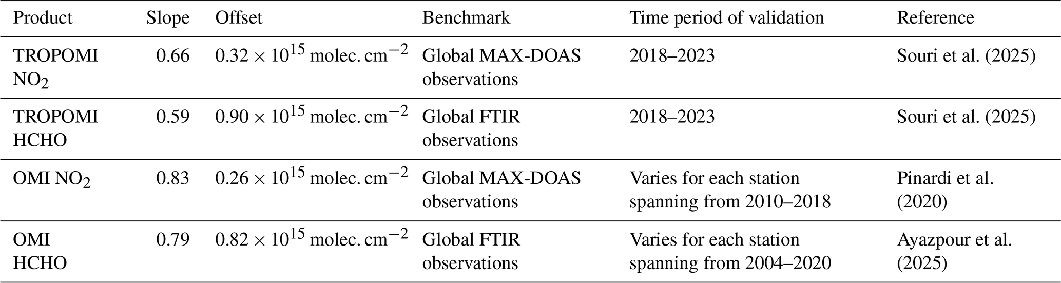
In order to remove large biases in both TROPOMI and OMI products, we bias correct their columns using the offset (additive term) and slope (multiplicative term) determined from a linear fit to paired MAX-DOAS/FTIR and these datasets, as described by Souri et al. (2025). The rationale for defining retrieval biases as a function of magnitude is to enhance correction factor generalizability across seasons and locations. We take advantage of three studies characterizing the bias correction factors, listed in Table 1. The application of these correction factors yields consistency across OMI and TROPOMI NO₂ and HCHO columns within 10 % (Sect. 4.4.4)

Table 1 The slopes and offsets derived from various validation studies used to bias correct the satellite retrievals employed in the parameterization of PO₃.

2.1.4 Surface albedo

To estimate near-surface photolysis rates of jO¹D (O₃+hv, < 350 nm) and jNO₂ (NO₂+hv, ∼ 400–500 nm) used in the parametrization of PO₃, we are required to provide reasonable surface albedo estimates (Sect. 2.4). We use a monthly Directionally Dependent Lambertian-Equivalent reflectivity (DLER) climatology derived from TROPOMI radiances at the spatial resolution of 0.125° × 0.125°; the product is in good agreement with the MODIS BRDF product (Tilstra et al., 2024). This climatology has two sets of values for both shortwave (328 nm) and longwave UV (463 nm) that are used separately for calculating jO¹D and jNO₂, respectively. We use only the isotropic part of the DLER product (named minimum_LER), which is added to an offset coefficient provided with the dataset.

2.2 Aircraft Measurements

The use of aircraft observations is twofold: first, they provide a vast number of measured geophysical variables suitable to simulate our observationally-constrained PO₃ training dataset (Sect. 3.1); second, they enable a rigorous validation of column-to-planetary boundary layer (PBL) conversion factors derived from a chemical transport model (Appendix B). We use the dataset compiled by Souri et al. (2025), who curated various aircraft campaigns measuring photolysis rates, meteorological variables, and atmospheric composition from varying atmospheric conditions, including urban/suburban settings (DISCOVER-AQs, and KORUS-AQ), high-vegetated regions (SENEX), and remote areas (INTEX-B and AToms). The sampling frequency varies from 10 to 30 s. More detailed information regarding the choice of instrument, gap filling, and data exclusion can be found in Souri et al. (2025).

2.3 MINDS simulations

We use a global chemical transport model simulation designed to support trace gas retrievals. The simulation, called Multi-Decadal Nitrogen Dioxide and Derived Products from Satellites (MINDS) (Fisher et al., 2024), was generated using the Goddard Earth Observing System (GEOS) Earth system model (Molod et al., 2015; Nielsen et al., 2017) equipped with the full chemistry Global Modeling Initiative (GMI) mechanism (Duncan et al., 2007; Strahan et al., 2007) and coupled with the Goddard Chemistry Aerosol Radiation and Transport (GOCART) aerosol module (Chin et al., 2002). The rapid radiative transfer model, which was designed for global climate models (GCMs) and is known as the Radiative Transfer Module for GCM (RRTMG), calculates the longwave and shortwave radiation influenced by aerosols simulated by GOCART, enabling the incorporation of the direct effects of aerosols on meteorological conditions (Nielsen et al., 2017). Meteorology is resolved using GEOS with several prognostic inputs, including water vapor, being constrained by MERRA-2 reanalysis using “replay” mode at 3-hourly basis (Orbe et al., 2017). The model is setup at c360 grid (0.25° × 0.25°) and covers the period of 1993 until the end of 2023. The model follows 72 hybrid sigma values ranging from the surface to 0.01 hPa.

Lightning production of NO is parametrized based on the simulated convection. The model uses the Monitoring Atmospheric Chemistry and Climate and CityZen (MACCity) inventory (Granier et al., 2011) of anthropogenic emissions downscaled to 0.1° × 0.1° using the Emissions Database for Global Atmospheric Research version 4.2 (EDGAR 4.2). These anthropogenic emissions change by year and month. Biomass burning emissions rely on the Fire Energetics and Emissions Research (FEER) dataset (Ichoku and Ellison, 2014). Biogenic emissions are modeled interactively by the Model of Emissions of Gases and Aerosols from Nature (MEGAN) v2.1 (Guenther et al., 2012). It is known that isoprene emissions in MEGANv2.1 are largely overestimated (Bauwens et al., 2016; Souri et al., 2020b), therefore they are scaled down by a factor of two.

2.4 TUV NCAR Photolysis Rates Look-up Table

To estimate jNO₂ and jO¹D, we refer to a detailed look-up table provided by the Framework for 0-D Atmospheric Modeling (F0AM) model (Wolfe et al. 2016). This table is developed for clear-sky conditions based on over 20 064 solar spectra calculations. The data encompasses a broad spectrum of solar zenith angles (SZA) from 0 to 90° in 5° increments, altitudes ranging from 0 to 15 km in 1 km steps, overhead total ozone columns from 100 to 600 DU in increments of 50 DU, and surface UV albedo values from 0 to 1 in 0.2 increments. These calculations were carried out using NCAR's Tropospheric Ultraviolet and Visible radiation model (TUV v5.2), along with cross sections and quantum yields from IUPAC and JPL (Wolfe et al., 2016). Information on SZA and surface elevation is obtained from the L2 TROPOMI/OMI granule data. Surface albedo is based on the TROPOMI DLER climatology (Sect. 2.1.4). The overhead total ozone columns are derived from MINDS simulations (Sect. 2.3). For any values that fall between the entries in the tables, we apply a linear interpolation method.

2.5 Empirical PO₃ estimates using LASSO

We will compare our new product (Sect. 3.2) to an empirical method developed by Souri et al. (2025), who took advantage of simulated PO₃ data constrained by aircraft measurements to parameterize PO₃ using four geophysical variables: NO₂, HCHO, jNO₂, and jO¹D. Their algorithm used a piecewise L1-regularized linear regression model known as Least Absolute Shrinkage and Selection Operator (LASSO). Since the algorithm was based on a linear model which was ill-suited for the non-linear ozone chemistry, it was necessary to linearize the parameterization using various thresholds for FNRs. Despite the method's simplicity, Souri et al. (2025) were able to reproduce approximately 88 % of the variance with low biases (less than 20 %) in observationally-constrained PO₃. Using the empirical method, they generated the first maps of PO₃ by combining bias-corrected TROPOMI HCHO and NO₂ columns, simulated photolysis rates, and a global transport model designed for the conversion from column measurements to the PBL.

To isolate the performance of the PO₃ estimator used in Souri et al. (2025) in comparison to the proposed algorithm in this study, we will ensure that the input variables, including the mixing ratios of HCHO and NO₂ within the PBL as well as the photolysis rates, remain identical for both the empirical product and our new algorithm. Hereafter, we will refer to this empirical product as “PO₃LASSO”.

3 Methodology

Figure 1 illustrates the three-stage process of our newly developed algorithm to operationally produce long-term maps of PO₃ within the PBL along with the sensitivity and error maps. The product is called “PO₃DNN”.

• Stage I. This stage serves as the foundation for the product, focusing on parameterizing PO₃ using a regularized Deep Neural Network (DNN). The training dataset, detailed in Sect. 3.1, is derived from an observationally-constrained F0AM box model that provides simulated PO₃ along with various atmospheric quantities directly or indirectly constrained by aircraft measurements. The decision to make use of aircraft data is based on two main factors: (i) they capture real-world atmospheric conditions across diverse parts of the atmosphere and various geographic regions, and (ii) the significant fluctuations inherent in the data rigorously test the DNN's capability to generalize (i.e., to fit the model through the data rather than merely to the data). However, a notable limitation of aircraft data is its restriction to specific atmospheric conditions. To address this, we have expanded the training dataset by perturbing the inputs to the F0AM model (Sect. 3.1), resulting in a synthetic dataset. This expanded training dataset is then used for validation, testing, and calibration of the DNN algorithm.

• Stage II. The objective of this stage is to prepare spatiotemporal geophysical variables necessary for the prediction of PO₃ (done in Stage III). We need five parameters on a global scale with daily frequency: jNO₂, jO¹D, HCHO, NO₂, and H₂O(v). To generate global daily maps of near-surface photolysis rates, we use the NCAR's look-up table as detailed in Sect. 2.4; this table relies on SZA, which varies with time and location, as well as surface UV-Vis albedo, ozone overhead columns, and surface altitudes. Both SZA and surface altitude are provided as auxiliary fields in the satellite L2 products. Ozone overhead columns are from MINDS. For surface UV-Vis albedo, we use two different wavelengths based on TROPOMI's climatology (Sect. 2.1.4). These calculations assume clear sky conditions, which are somewhat achieved by the effective cloud fraction thresholds derived from both the OMI and TROPOMI products. Our algorithm uses HCHO and NO₂ columns obtained from OMI or TROPOMI, which are bias-corrected against ground remote sensing data. These measurements are then transformed into the mixing ratios in the PBL region using the vertical distribution of HCHO and NO₂ profiles simulated by MINDS. The final variable is the average number of water vapor (H₂O(v)) molecules per cubic meters in the PBL region at the satellite overpass time, which is obtained directly from the MINDS simulation. It is important to note that the MINDS simulation is based on constraints from MERRA-2 reanalysis, underscoring that the H₂O(v) simulations are constrained by many observations.

• Stage III. In the final stage, we predict PO₃, generate sensitivity maps, and provide both systematic and random errors associated with these estimates. To create PO₃ maps, we input the five parameters from Stage II into the DNN model developed in Stage I. To generate the sensitivity maps of PO₃ in relation to NO₂ and HCHO, we apply perturbations to NO₂ and HCHO based on the methodology described in Sect. 3.3. These perturbations also serve another purpose which is to propagate the errors associated with the retrievals of HCHO and NO₂, as well as their corresponding conversion factors from MINDS into the final product. A comprehensive explanation of the error budget and characterization can be found in Sect. 3.4.

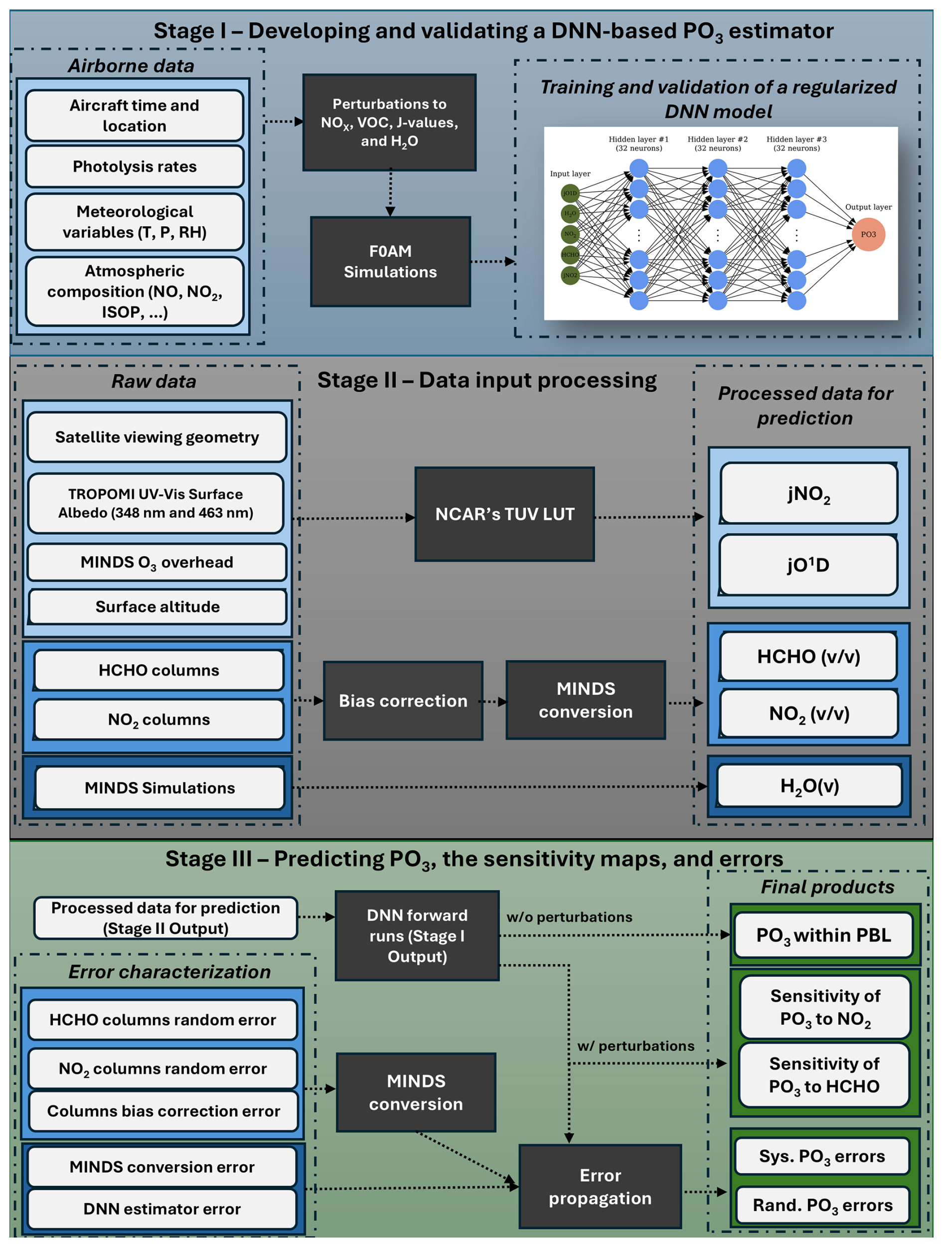
Figure 1 Processing stages developed to operationally generate PO₃ and sensitivity maps along with daily frequency errors on a global scale. Stage I aims to establish a regularized DNN model based on synthetic and real-world aircraft measurements. Stage II prepares the necessary satellite-based input features used for PO₃ prediction in Stage III. Stage III feeds the DNN model with Stage II values and some statistical error analysis to generate the final product.

While we perform Stage I only once to establish a PO₃ estimator, we need to run Stage II and III for any desired location/time or spatial resolution. The need to operationally run these two stages has motivated us to create an open-source and object-oriented Python package called ozonerates v1.0 (Souri and Gonzalez Abad, 2025), which is capable of running all steps while leveraging parallel computation.

3.1 Training dataset generation using F0AM box model

To establish a relationship between several geophysical variables related to PO₃, we use F0AM version 4 box model (Wolfe et al., 2016). This model is capable of simulating detailed chemical kinetics based on user inputs regarding meteorological variables, atmospheric compositions, and photolysis rates. F0AM uses a solver for ordinary differential equations (ODEs) designed for stiff systems, which allows it to determine the chemical evolution of all species included in the selected chemical mechanism. We adhere to previous configurations that apply the Carbon Bond 6 (CB06, r2) chemical mechanism within F0AM (Souri et al., 2020a; Souri et al., 2023a; Souri et al., 2025). The model is constrained by data collected during aircraft campaigns, including meteorological data, photolysis rates, and various trace gas concentrations. Additional details regarding the selection of instruments, bias corrections for photolysis, choices of dilution factors, and other configurations can be found in Souri et al. (2025). We incorporate data from seven aircraft campaigns, including DISCOVER-AQ (Texas, Washington D.C., Colorado), KORUS-AQ, ATOMs, INTEX-B, and SENEX, to further constrain the model. Souri et al. (2025) demonstrated that this setup effectively reproduces several unconstrained yet measured compounds, such as HCHO, HO₂, OH, and PAN; moreover, the performance of the model was on par with other studies (e.g., Brune et al., 2020; Brune et al., 2022; Miller and Brune, 2022), indicating that it is a suitable model setup for understanding local ozone chemistry. This model-derived dataset consists of ∼ 134 000 points.

A limitation to the training dataset prepared by Souri et al. (2025) originates from the fact that only a subset of atmospheric conditions could be observed by the suborbital missions. A remedy for this limitation is to synthetically regenerate data by systematically perturbing several of the inputs used in the F0AM model. As a result, we apply a scaling factor, ranging from 0.1 up to 10 in 12 evenly-spaced steps, separately to NO_x, VOCs, H₂O(v), and photolysis rates. This expands the dataset to ∼ 6.4 million datapoints, covering a much wider range of atmospheric states.

Once the simulations are done, we determine simulated PO₃ by:

$$\begin{array}{}\text{(1)}& {\mathrm{PO}}_{\mathrm{3}}={\mathrm{FO}}_{\mathrm{3}}-{\mathrm{LO}}_{\mathrm{3}}\end{array}$$

where LO₃ is all possible chemical loss pathways of ozone (negative stoichiometric multiplier matrix) and FO₃ is all possible chemical pathways producing ozone molecules (positive stoichiometric multiplier matrix). This equation is also known as ozone tendency. This definition simplifies intercomparison with estimates derived from different chemical mechanisms by eliminating the requirement to explicitly match individual production and loss terms, which often exhibit inconsistencies across mechanisms, especially in their treatment of peroxy radicals. The calculation of PO₃ is under a steady-state assumption.

3.2 DNN architecture and configuration

The overall architecture of the DNN model is portrayed in Fig. 2. The design consists of three fully-connected hidden layers each having 32 neurons. The neurons are equipped with rectified linear unit (ReLU) activation functions. The training dataset (∼ 6.4 millions) is split into 20 % test, 24 % validation, and 56 % training. Training inputs to the parametrization consists of HCHO, NO₂, jO¹D, jNO₂, and H₂O(v). Prior to the training, we normalize them, such that each feature (x) is rescaled according to $x^{\prime }=\frac{x-\mathit{\mu }}{\mathit{\sigma }}x$, where μ and σ represent the mean and standard deviation of the feature, respectively, ensuring a mean of zero and a variance of one. The optimization (training) of the DNN follows the backpropagation rule armed with Adaptive Moment Estimation (ADAM) optimizer which is known to perform well with noisy data (Kingma and Ba, 2017). The initial learning rate is set to 10⁻⁵. We use 500 epochs. The loss function (L) of the optimalization problem is:

$$\begin{array}{}\text{(2)}& L={\displaystyle \frac{\mathrm{1}}{\mathrm{2}}}\sum _{k=\mathrm{1}}^N(y_k-o_k{)}^{\mathrm{2}}+\mathit{\lambda }\sum _{i=\mathrm{1}}^p{w}_i^{\mathrm{2}}\end{array}$$

where the first term on the right side represents the mean squares error (MSE) of the prediction derived from difference between the target PO₃ (y) and the predicted PO₃ (o). N represents the number of training datapoints. The second term is L2-regularization with a factor of λ to reduce the squares of p number of neuron weights (w).

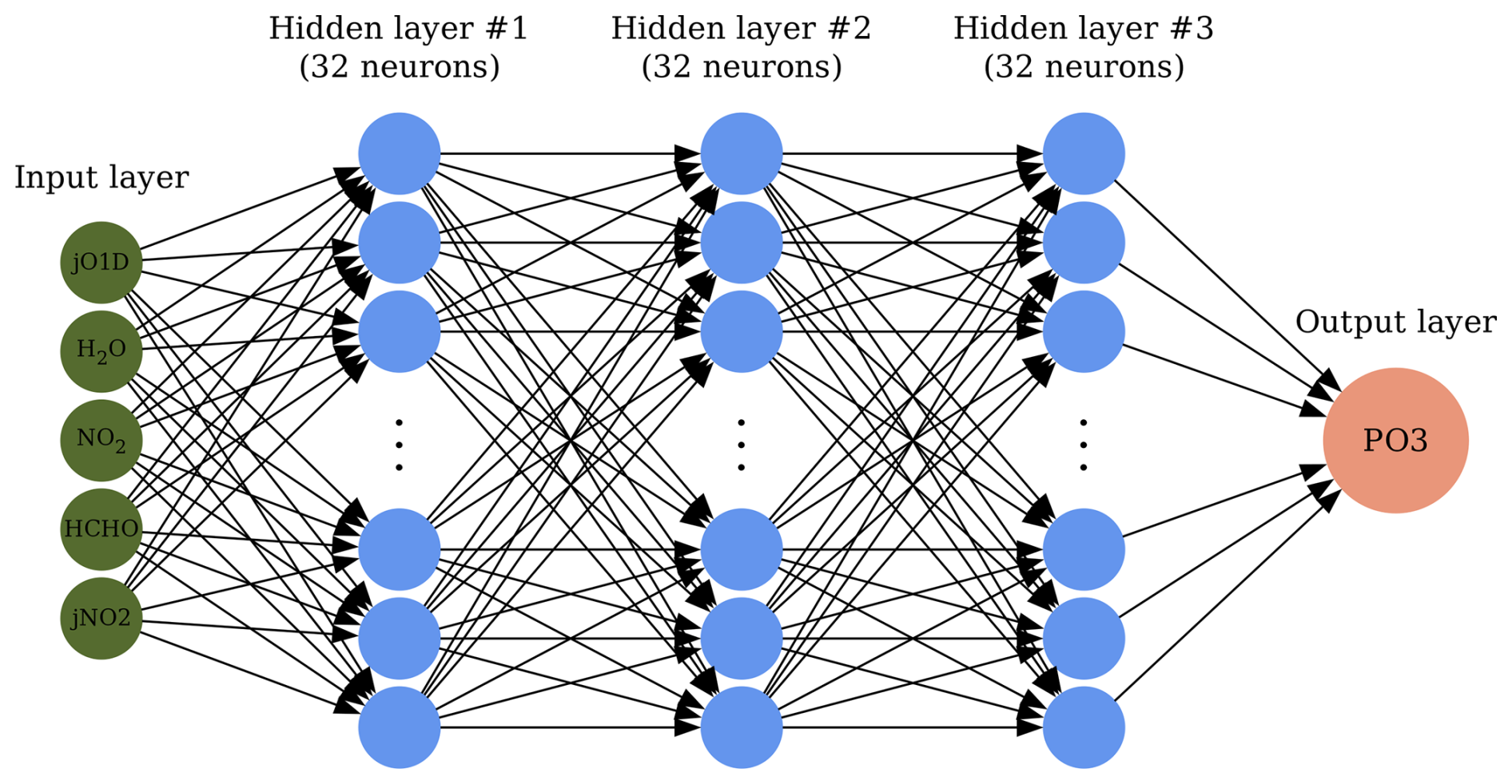
Figure 2 The architecture of the DNN model. The model contains three hidden layers with 32 neurons each.

An important aspect of this optimization is the use of L2 regularization, which effectively helped us determine the optimal number of hidden layers and neurons. L2 regularization penalizes the cost function if an illusion of high prediction accuracy (the first term) is achieved with excessive variance in the solution (weights). Failing to balance the prediction error and the solution variance can lead to overfitting, which harms model performance in two ways: (i) it results in erroneous predictions for atmospheric conditions that fall outside the training dataset; (ii) it diminishes the physical interpretability of the statistical model because of large fluctuations in the weights, a common issue in regression models known as collinearity. When we used too many neurons or layers, the regularization penalized the weights, causing a substantial proportion to approach zero (not shown), indicating that those neurons were unnecessary. However, incorporating regularization does have some drawbacks: (i) it requires a smaller initial learning rate (set to 10⁻⁵) to avoid falling into local minima, which demands more computational resources; and (ii) the regularization factor also needs to be optimized. We find that a value of λ= 10⁻⁵ provides the best results among the set of values [10⁻⁴, 10⁻⁵, and 10⁻⁶], based on the symmetry in the statistical distributions of the test residuals, MSE, and the overall level of physical interpretability observed in the sensitivity tests.

The implementation of the DNN model is done using the open-source TensorFlow application programming interface (API) package in Python (Abadi et al., 2016). To thoroughly validate the performance of this model from various angles we (i) compare the DNN prediction with the test data using various standard metrics, (ii) investigate the evolution of the loss function derived from both the training set and the validation one over epochs, (iii) study the physical explanation of the response of PO₃ to NO₂ and HCHO, water vapor, and photolysis rates, and (iv) finally compare the DNN results to PO₃LASSO. We will use a number of statistical metrics, including the coefficient of the determination (R²), mean bias, mean square error, mean absolute error, and root mean square error (RMSE), to carry out the quantitative assessment (Sect. 4.1).

3.3 Sensitivity calculations

To elucidate the response of PO₃ to its inputs, we calculate the semi-normalized sensitivities through the finite difference method:

$$\begin{array}{}\text{(3)}& {\mathrm{SPO}}_{{\mathrm{3}}_i}={\displaystyle \frac{[{\mathrm{PO}}_{\mathrm{3}}{]}_i^{\mathrm{110}\mathit{\%}}-[{\mathrm{PO}}_{\mathrm{3}}{]}_i^{\mathrm{90}\mathit{\%}}}{\mathrm{0.2}}}\end{array}$$

where $[{\mathrm{PO}}_{\mathrm{3}}{]}_i^{\mathrm{110}\mathit{\%}}$ and $[{\mathrm{PO}}_{\mathrm{3}}{]}_i^{\mathrm{90}\mathit{\%}}$ are PO₃ from perturbing input parameters (i= 1 for NO₂, and i= 2 for HCHO) by 1.1 and 0.9 scaling factors. A mathematical proof showing that these sensitivity calculations are equivalent to the directional derivative is provided in Appendix A.

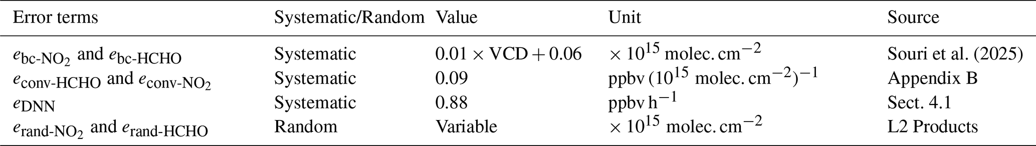
3.4 Error budget and characterization

Since the PO₃DNN integrates atmospheric models, satellite trace gas retrievals, ground remote sensing, and a machine learning approach, it contains various sources of errors, some of which will be formulated in this section. Spatially and temporally averaging satellite-based products is a common practice to reduce noise and fill gaps; therefore, we attempt to separate systematic errors (irreducible by averaging) from random ones (reducible by averaging). We assign the total PO₃ within PBL region error (e_total) based on the following equation:

$$\begin{array}{}\text{(4)}& e_{\mathrm{total}}=\sqrt{e_{\mathrm{syst}}^{\mathrm{2}}+e_{\mathrm{rand}}^{\mathrm{2}}}\end{array}$$

where e_syst and e_rand are systematic and random errors associated with PO₃ estimates. Systematic errors account for the errors associated with the bias correction of OMI and TROPOMI against ground remote sensing retrievals (e_{HCHO_bias_c} and $e_{{\mathrm{NO}}_{\mathrm{2}}\mathrm{\_}\mathrm{bias}\mathrm{\_}\mathrm{c}}$), the model-based conversion of columns to the PBL mixing ratios ($e_{\mathrm{HCHO}\mathrm{\_}\mathrm{conversion}},e_{{\mathrm{NO}}_{\mathrm{2}}\mathrm{\_}\mathrm{conversion}}$), and the DNN estimator error (e_DDN), and are given by:

$$\begin{array}{}\text{(5)}& {\displaystyle }\begin{array}{rl}& e_{\mathrm{syst}}=\\ & \sqrt{e_{\mathrm{HCHO}\mathrm{\_}\mathrm{bias}\mathrm{\_}\mathrm{c}}^{\mathrm{2}}+e_{{\mathrm{NO}}_{\mathrm{2}}\mathrm{\_}\mathrm{bias}\mathrm{\_}\mathrm{c}}^{\mathrm{2}}+e_{\mathrm{HCHO}\mathrm{\_}\mathrm{conversion}}^{\mathrm{2}}+e_{{\mathrm{NO}}_{\mathrm{2}}\mathrm{\_}\mathrm{conversion}}^{\mathrm{2}}+e_{\mathrm{DNN}}^{\mathrm{2}}}\end{array}\text{(6)}& {\displaystyle }{e}_{\mathrm{HCHO}\mathrm{\_}\mathrm{bias}\mathrm{\_}\mathrm{c}}^{\mathrm{2}}={\left({\displaystyle \frac{\partial {\mathrm{PO}}_{\mathrm{3}}}{\partial \mathrm{HCHO}}}\cdot \mathit{\gamma }\cdot e_{\text{bc-HCHO}}\right)}^{\mathrm{2}}\text{(7)}& {\displaystyle }{e}_{{\mathrm{NO}}_{\mathrm{2}}\mathrm{\_}\mathrm{bias}\mathrm{\_}\mathrm{c}}^{\mathrm{2}}={\left({\displaystyle \frac{\partial {\mathrm{PO}}_{\mathrm{3}}}{\partial {\mathrm{NO}}_{\mathrm{2}}}}\cdot \mathit{\gamma }\cdot e_{{\text{bc-NO}}_{\mathrm{2}}}\right)}^{\mathrm{2}}\text{(8)}& {\displaystyle }{e}_{\mathrm{HCHO}\mathrm{\_}\mathrm{conversion}}^{\mathrm{2}}={\left({\displaystyle \frac{\partial {\mathrm{PO}}_{\mathrm{3}}}{\partial \mathrm{HCHO}}}\cdot {\mathrm{VCD}}_{\mathrm{HCHO}}\cdot e_{\text{conv-HCHO}}\right)}^{\mathrm{2}}\text{(9)}& {\displaystyle }{e}_{{\mathrm{NO}}_{\mathrm{2}}\mathrm{\_}\mathrm{conversion}}^{\mathrm{2}}={\left({\displaystyle \frac{\partial {\mathrm{PO}}_{\mathrm{3}}}{\partial {\mathrm{NO}}_{\mathrm{2}}}}\cdot {\mathrm{VCD}}_{{\mathrm{NO}}_{\mathrm{2}}}\cdot e_{{\text{conv-NO}}_{\mathrm{2}}}\right)}^{\mathrm{2}}\end{array}$$

where γ is the conversion factor of the satellite total to the PBL columns translation based on MINDS and the formulation by Souri et al. (2025); e_bc-HCHO and $e_{{\text{bc-NO}}_{\mathrm{2}}}$, in column units, are calculated following the formulation from Souri et al. (2025) who used the errors of slope and offset obtained from the comparison of satellite VCDs to ground remote sensing benchmarks; e_conv-HCHO and $e_{{\text{conv-NO}}_{\mathrm{2}}}$ are quantified by validating the simulated conversion factors compared to those of aircraft vertical spirals (Appendix B). The unit for these two errors is ppbv per the column unit; accordingly, we multiply these terms to satellite VCDs. The last term in Eq. (5) is a fixed systematic error associated with the DNN estimates which will be quantified based on the MSE of the DNN prediction. Both $\frac{\partial {\mathrm{PO}}_{\mathrm{3}}}{\partial \mathrm{HCHO}}$ and $\frac{\partial {\mathrm{PO}}_{\mathrm{3}}}{\partial {\mathrm{NO}}_{\mathrm{2}}}$ are derived from the sensitivity calculations from Eq. (3) divided by the satellite columns. All error terms in Eqs. (6)–(9) are spatially and temporally invariant, but the derivatives vary from pixel to pixel resulting in spatiotemporally-varying systematic errors.

Random errors originate from the uncertainty estimates coming with the TROPOMI and OMI L2 products and are somewhat reducible by averaging, and are given by:

$$\begin{array}{}\text{(10)}& \begin{array}{rl}& e_{\mathrm{rand}}=\\ & \sqrt{{\left({\displaystyle \frac{\partial {\mathrm{PO}}_{\mathrm{3}}}{\partial \mathrm{HCHO}}}\cdot \mathit{\gamma }\cdot e_{\text{rand-HCHO}}\right)}^{\mathrm{2}}+{\left({\displaystyle \frac{\partial {\mathrm{PO}}_{\mathrm{3}}}{\partial {\mathrm{NO}}_{\mathrm{2}}}}\cdot \mathit{\gamma }\cdot e_{{\text{rand-NO}}_{\mathrm{2}}}\right)}^{\mathrm{2}}}\end{array}\end{array}$$

where e_rand-HCHO and $e_{{\text{rand-NO}}_{\mathrm{2}}}$ are random retrieval errors. All terms in Eq. (10) vary by time and location.

Table 2 summarizes the numbers used in the above equations and their origin.

Table 2 Values used in error calculations.

It is important to acknowledge that the defined total error budget here is only a good guess and optimistic. Some underlying sources of error, which are difficult to quantify, are not included. For example, errors related to the training dataset derived from the F0AM model are challenging to assess because of the lack of PO₃ measurements. We assume other inputs to the PO₃ parametrization, such as the monthly climatology TROPOMI surface albedo to be error-free. Additionally, all datasets used to estimate PO₃ contain spatial representation errors (Souri et al., 2022), which are difficult to measure without knowing their true state of global spatial variability. Moreover, we do not consider correlated errors among HCHO and NO₂ retrievals. It is worth noting that some of the inputs such as H₂O(v) and the overhead ozone column have minimal biases because of MINDS simulations being observationally constrained (Fisher et al., 2024; Souri et al., 2024).

There are also assumptions regarding the equations mentioned earlier. For instance, it is assumed that the validation of conversion factors can account for all systematic issues related to the vertical distribution of NO₂ and HCHO in MINDS. Furthermore, we presume that the reported retrieval errors are mostly random; however, this is not the case (Eskes and Boersma, 2003; Boersma et al., 2018) and distinguishing between these errors is not straightforward.

Another source of uncertainty arises from partially cloudy pixels and aerosols, which can introduce errors in calculated photolysis rates. While we successfully filtered out cloud cover and strong aerosol loadings (e.g., from wildfires) using effective cloud fraction thresholds, some aerosol or cloud-contaminated pixels may pass cloud screening due to low optical depth or height characteristics. Rigorously quantifying the errors coming from these effects would require running a radiative transfer model with detailed three-dimensional optical properties of clouds and aerosols on a global scale, particularly critical for aerosols, which can have complex effects on photolysis rates depending on their absorption and scattering properties and vertical distribution. Unfortunately, such comprehensive datasets are typically limited to the narrow swaths of spaceborne lidar observations, which themselves carry substantial uncertainties (Thorsen and Fu, 2015). While these complications cannot be entirely avoided, particularly for aerosol effects, users can apply additional quality control measures by filtering pixels using aerosol optical depth retrievals from TROPOMI, OMI, or other sensors to more rigorously identify contaminated observations.

In case of oversampling of the PO₃ product both temporally and spatially, the total error will be given by:

$$\begin{array}{}\text{(11)}& e_{\mathrm{total}\mathrm{\_}\mathrm{oversampled}}=\sqrt{{\displaystyle \frac{\mathrm{1}}{m}}\sum e_{\mathrm{syst}}^{\mathrm{2}}+{\displaystyle \frac{\mathrm{1}}{m^{\mathrm{2}}}}\sum e_{\mathrm{rand}}^{\mathrm{2}}}\end{array}$$

where m is the total number of samples. Equation (11) suggests that the systematic errors are persistent across all samples and are not reducible by averaging, whereas the random errors become smaller by root square of samples. In this equation, the assumption is that the root-mean-square of the systematic errors is a good approximation of the systematic errors in the oversampled data because they are independent of each other.

4 Results and Discussion

In this section, we begin by validating and contrasting PO₃DNN against PO₃LASSO. Following that, we use OMI to investigate the spatiotemporal variability of PO₃ and its sensitivity to photolysis rates, HCHO, and NO₂ globally. We provide an application of data to understand the global long-term trends PO₃ derived from OMI. Afterward, we offer a comprehensive global view of the PO₃ estimates algorithm by integrating data from the TROPOMI compared with that one based on OMI. Finally, we document the total error budget of the products.

4.1 DNN performance

We investigate the predictive power of the DNN algorithm against both validation and test data for each air quality campaign or the entire aircraft dataset (Sect. 2.2). All training datasets described in Sect. 3.1 are used in this stage. Except for the early stages of training, both training and validation curves, explaining the evolution of the prediction against the number of epochs corresponding to the number of iterations of training the network for one cycle, closely follow each other, indicating that we possibly do not have overfitting issues (Fig. S11 in the Supplement). The curves are fairly smooth, resulting from using the ADAM optimizer with a strictly small learning rate initially. Both curves converge to RMSE below 0.88 ppbv h⁻¹ which we use to assign the error of PO₃DNN prediction in Eq. (5).

PO₃DNN has promising skill at predicting PO₃ across various atmospheric conditions. Figure 3 presents a comparison of the predicted PO₃ values against observationally-constrained F0AM values for the test data for each suborbital mission. A similar comparison, which includes all data points measured during each mission, can be found in Fig. S12. The primary reason for highlighting the test data is that they have never been used to fine-tune the DNN parameters. There is a strong correlation between the predictions and the benchmarks across most campaigns for both the test data points (Fig. 3) and the complete set of aircraft measurements (Fig. S12). Notably, the slope for the “All” test dataset is close to the unity line. The DNN algorithm can reproduce over 96 % of the variance in the test data. Similar to the approach of Souri et al. (2025), we completely exclude each suborbital mission from the training dataset and use it as an independent benchmark to evaluate the model's performance. The resulting accuracy is comparable to that achieved when 56 % of the data are used for training, indicating that the PO₃ parameterization has reached a high degree of generalization (Fig. S13).

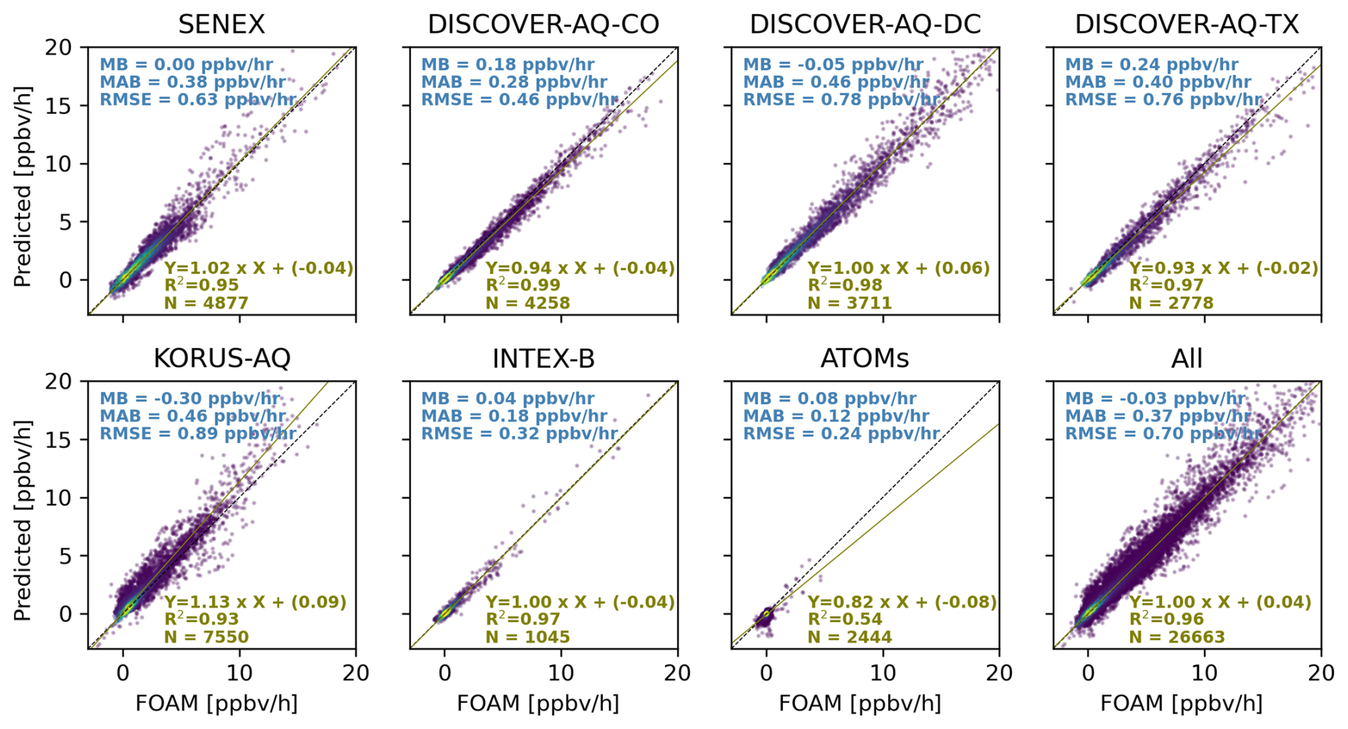
Figure 3 Scatterplots comparing observationally-constrained F0AM model PO₃ and the predictions that were based on the DNN for the test data from each air quality campaign. The test data have never been used for hyper tuning the algorithm. “All” denotes all test data.

The model performs significantly better than PO₃LASSO over INTEX-B compared to LASSO (as shown in Fig. 7 in Souri et al., 2025). While the DNN's performance over the ATom campaigns is less impressive than in other areas, it still represents a considerable improvement over LASSO, which was unable to reproduce PO₃ in pristine regions (R²<0.05). One key factor contributing to this improvement is the inclusion of H₂O(v) in the input. Various parameters, including HO_x, are known to influence PO₃ in remote regions, but these factors were not included in our parametrization. The method does not artificially inflate results by introducing non-physical relationships in remote regions; the inability of the DNN to fully explain PO₃ during AToms suggests that it does not force unrealistic relationships between PO₃ and the inputs to completely align with the F0AM results, leaving areas for future improvement in parametrization over remote regions.

4.2 Advantages of PO₃DNN over PO₃LASSO

There are primarily four major benefits of PO₃DNN over PO₃LASSO that make the former parameterization a superior algorithm. The discussion of these advantages is as follows:

• Higher predictive power. PO₃LASSO predicted PO₃ for all datapoints collected from the suborbital missions with a R²= 0.88, RMSE = 1.2 ppbv h⁻¹, and a slope of 0.87 (Souri et al., 2025), whereas PO₃DNN reproduced the exact datapoints (Fig. S12) with a R²= 0.96, RMSE = 0.7 ppbv h⁻¹, and a slope of 1.00. Furthermore, as shown in Fig. 3, PO₃DNN has a great degree of generalization for datapoints outside of the training/validation data points. Consequently, these statistics suggest that DNN is a more powerful predictor.

• Better representation of PO₃ over remote regions. One notable limitation of PO₃LASSO was its inadequate representation of PO₃ in remote regions, such as during the ATOMs or INTEX-B campaigns. This led Souri et al. (2025) to entirely mask PO₃ estimates below 1 ppbv h⁻¹. In these remote areas, PO₃ is typically influenced by the reactions between ozone and HO_x in addition to jO¹D and H₂O. While Souri et al. (2025) attempted to incorporate H₂O into the LASSO parametrization, the algorithm assigned a zero coefficient to this parameter because of the use of the L1-regularization term. This term typically assigns a zero coefficient for a geophysical variable that is either irrelevant to the target or shows strong non-linear relationship with the target. PO₃LASSO did not factor in H₂O(v) because H₂O(v) exhibits a non-linear relationship with PO₃ – although the reaction between O¹D and H₂O can suppress ozone formation through the removal of O¹D, it produces two molecules of OH regenerating ozone in polluted places (Bates and Jacob, 2020). Consequently, the non-linear relationship between H₂O and PO₃ is one that LASSO was unable to capture. While we could have addressed this by dividing the training dataset into different humidity levels (i.e., dry and humid), such an approach would have resulted in more discretization in the parametrization. Conversely, PO₃DNN can consider the non-linear relationship between H₂O and PO₃ without the need for empirical linearization. We observe a significant improvement in predicted PO₃ for both AToms and INTEX-B campaigns compared to Souri et al. (2025).

• Diminished satellite error effects. The reliance of PO₃LASSO on FNR increases the contamination of PO₃ predictions from satellite random noise. This primarily occurs because satellite errors associated with HCHO and NO₂ adversely influence FNR (see Fig. 12 in Souri et al., 2023a), resulting in noise in the empirical linearization approach used in PO₃LASSO. Even if we assume that all inputs to the PO₃LASSO parameterization, except for FNR, are error-free, the inherent randomness from choosing among four different sets of equations segregated by the noisy FNR will still feed noise into the final estimate. Although PO₃DNN is inevitably influenced by satellite errors because of its dependence on HCHO and NO₂ columns, it does not exacerbate these errors because it operates independently of FNR. To demonstrate this tendency, Fig. 4 shows the global PO₃ random error maps induced by OMI HCHO and NO₂ retrieval random errors averaged in June 2006. We use identical inputs and errors for both algorithms. Figure 4 is evidence of the diminished contamination of satellite random errors in PO₃DNN as compared to PO₃LASSO. The error differences tend to be larger over clean areas, because FNR random errors are higher when both HCHO and NO₂ levels are small.

• Continuity. It is known that neural networks equipped with three hidden layers can well approximate almost any high-dimensional non-linear function (Shen et al., 2021). An important superiority of PO₃DNN over PO₃LASSO lies in the strength of the DNN algorithm at approximating high-dimensional non-linear relationships between PO₃ and HCHO (a proxy for VOCR), NO₂ (a proxy for reactive nitrogen), jNO₂ and jO¹D (a proxy for photochemistry), and H₂O. While some of these non-linearities were reasonably approximated in PO₃LASSO by empirically segregating the chemical conditions using FNR, the non-linear ozone photochemistry can go beyond the dependency on VOCs and NO_x levels. In fact, the relationship between PO₃ and VOCs and NO_x can behave non-linearly depending on the available light and water vapor as discussed in Sect. 4.3. This indicates that traditional linear models, such as those using $\mathrm{VOCR}/{\mathrm{NO}}_x$ (or $\mathrm{HCHO}/{\mathrm{NO}}_{\mathrm{2}}$) ratios, often fall short in capturing this complexity because of the continuous and non-linear nature of these relationships.

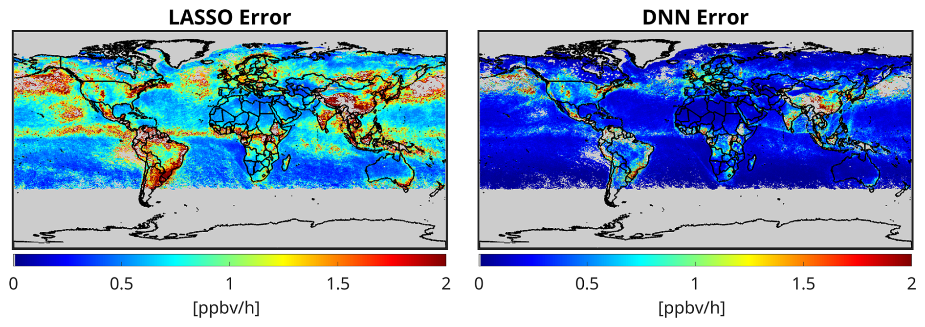
Figure 4 The comparison of the effect of satellite random errors in HCHO and NO₂ on PO₃ predictions based on PO₃LASSO and PO₃DNN algorithms in June 2006. The data used for generating these maps are based on OMI retrievals.

4.3 PO₃DNN can capture non-linear PO₃ chemistry as a function of pollution, light, and humidity

To further elaborate on the capability of PO₃DNN to reasonably respond to variations in its five major parameters in a mathematically continuous fashion, we create six isopleths, each specifically designed to represent a particular atmospheric condition listed in Table 3. These isopleths are based on perturbing HCHO and NO₂ in PO₃DNN and are shown in Fig. 5.

Table 3 Six different atmospheric conditions defined to understand the response of PO₃ to HCHO and NO₂ changes.

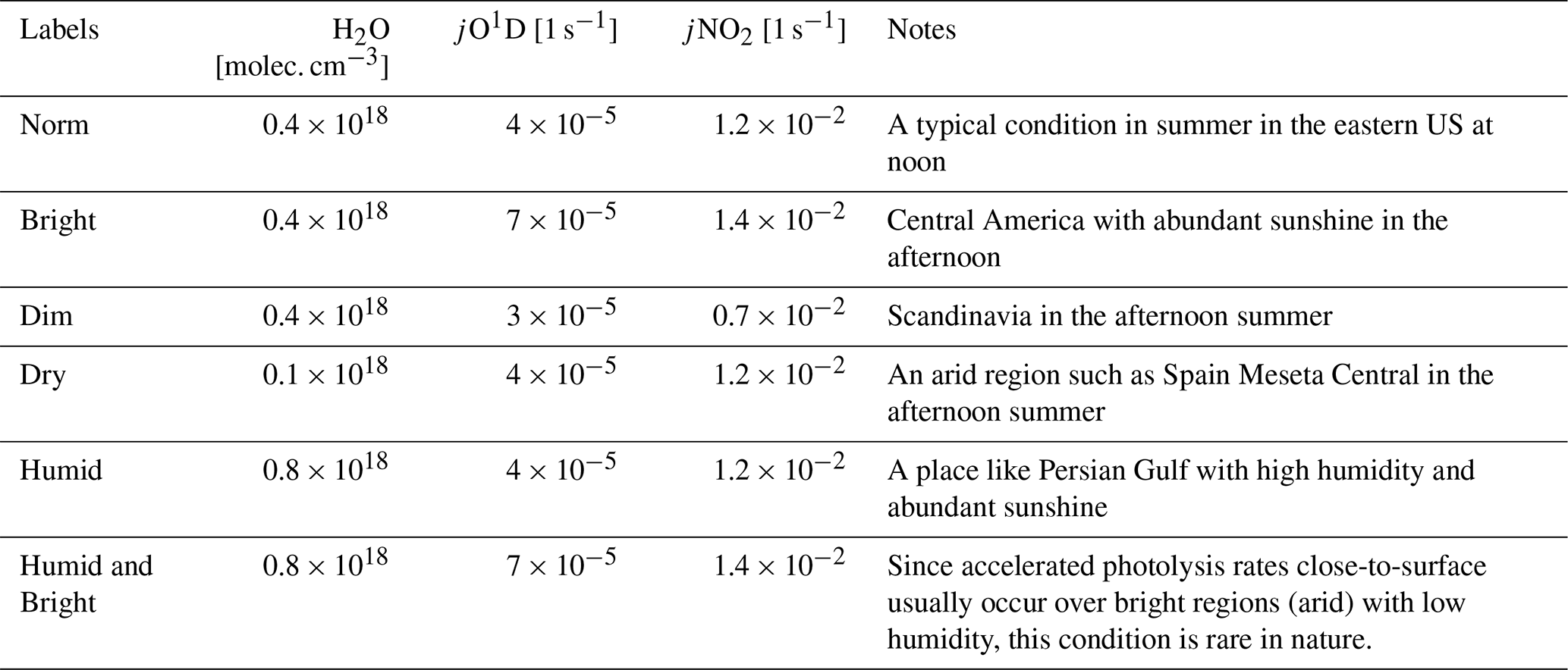
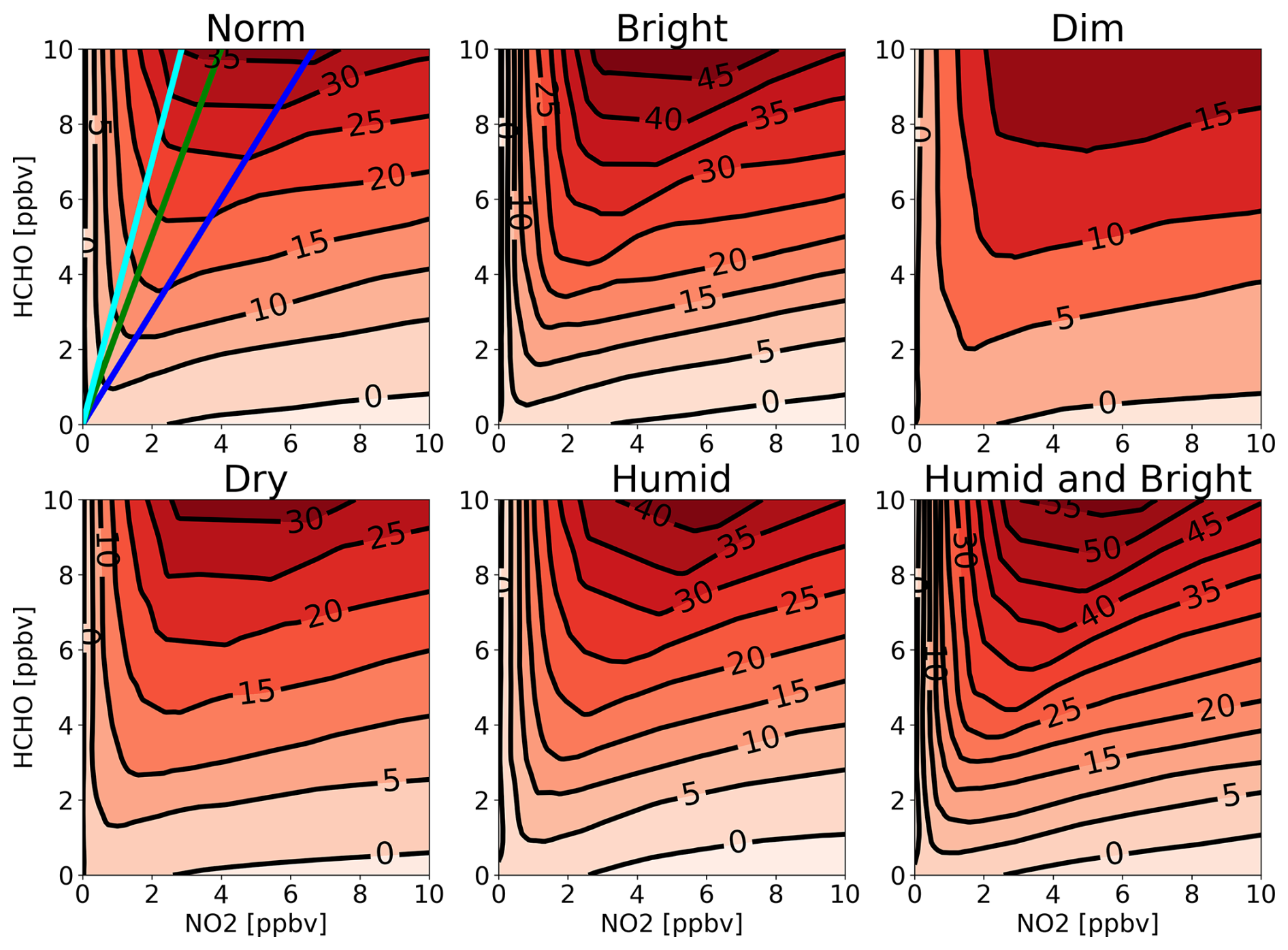
Figure 5 The contour maps of PO₃ isopleth generated by PO₃DNN algorithm for six different atmospheric conditions defined in Table 3. In the first subplot, blue, green, and cyan lines indicate FNR = 1.5, 2.5, and 3.5, respectively. Numbers on isopleths are in ppbv h⁻¹.

It is immediately apparent that the hyperbolic shape of the PO₃ curve relative to NO₂ and HCHO can be recreated by our algorithm, displaying a positive response to both HCHO and NO₂ on the right and left sides of the ridgelines. This observation underscores the effective parametrization of the non-linearities in ozone photochemistry achieved through the DNN algorithm. In the subplot representing normal conditions, we overlaid three lines indicating FNR values of 1.5 (blue), 2.5 (green), and 3.5 (cyan). Souri et al. (2025) used these lines to determine various coefficients in the PO₃LASSO parameterization. For instance, the derivative of PO₃ with respect to NO₂ was determined to be −0.14 ppbv h⁻¹ for FNR < 1.5 but increased to 6.54 ppbv h⁻¹ for FNR > 3.5. However, in practice, the thickness and curvature of the PO₃ isopleths vary based on the prevailing atmospheric conditions, implying that the derivatives cannot consistently retain the same values across the broad range of conditions.

In bright conditions, not only do we observe a significantly accelerated response of PO₃ compared to the norm at identical NO₂ and HCHO concentrations, but the responses of PO₃ to these two compounds also become more pronounced. Conversely, in dim conditions, both the magnitudes and responses are weaker.

These results underscore the importance of including photolysis rates in ozone sensitivity analysis, rather than relying solely on FNR in former studies. For example, a lower FNR in the morning (∼ 09:30 LST) compared to the afternoon may wrongly suggest that PO₃ would become more sensitive to VOCs earlier in the day. However, decreased light in the morning reduces the sensitivity of PO₃ to VOCs, despite a lower FNR (Sect. S1).

The contrast between dry and humid isopleths suggests that the presence of H₂O(v) enhances PO₃ when abundant NO₂ and HCHO are present. This trend is similarly observed in the F0AM model, as depicted in Figure S4, indicating that an increase in H₂O(v) over polluted regions (arbitrarily defined as HCHO × NO₂ > 10) increases PO₃. Nonetheless, more humidity suppresses PO₃ especially where VOC is limited and NO₂ is elevated possibly because the generated OH molecules from O¹D + H₂O(v) predominantly react with elevated NO₂.

Lastly, we see the highest PO₃ rates recorded among all scenarios under a hypothetical condition characterized by high humidity and photolysis rates. This condition is rare in nature because large amounts of H₂O(v) (0.8 × 10¹⁸ molec. cm⁻³) are confined to marine regions where surface reflectivity is low; nonetheless, an intuitive tendency from PO₃DNN suggests that the algorithm does not create non-physical extrapolation values.

4.4 PO₃ Maps and Sensitivities using OMI and TROPOMI: A General View, Long-term analysis, Intercomparisons, and Error Analysis

4.4.1 Global PO₃ and Seasonality using OMI in 2005–2007

Figure 6 shows the global distribution of PO₃ rates averaged over a quarter-degree in 2005–2007, using OMI HCHO and NO₂ retrievals. It also includes whisker-box plots highlighting seasonal variations in PO₃ for selected regions and cities. We selected the 2005–2007 timeframe for this analysis because the OMI data were free from degradation issues, including the row anomaly. The map indicates accelerated PO₃ rates across heavily polluted regions, such as cities in the Middle East, Asia, the U.S., Central Europe, and Africa, aligning with what we observed in Souri et al. (2025). While some areas exhibit significant seasonal fluctuations, others show little variability throughout the seasons. Notably, the east coast of the U.S., Central Europe, China, Tehran, and Johannesburg experience peak PO₃ rates in summer. This pattern is primarily attributed to enhanced photochemistry and the elevated sensitivity of PO₃ to NO_x, driven by increases in $\mathrm{VOCR}/{\mathrm{NO}}_x$ (Souri et al., 2025).

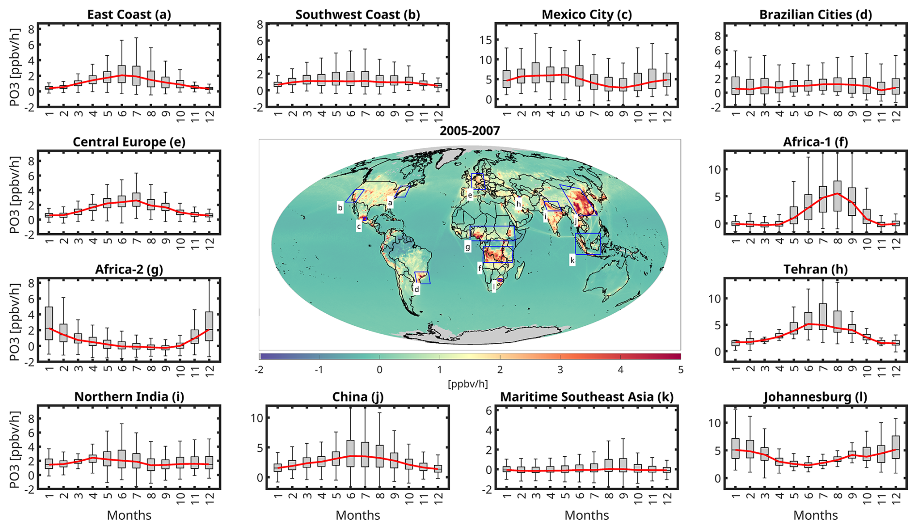
Figure 6 (center) The averaged global PO₃ map at 0.25° × 0.25° in 2005–2007 based on the new algorithm. OMI data are used to populate HCHO and NO₂ abundance. (margins) the whisker-box plots of PO₃ seasonality over various selected regions. In the box plot, the central red line shows the median, and the top and bottom edges of the box show the 25th (q₁) and 75th (q₃) percentiles. The dark solid lines at the very beginning and the end of each plot show the minimum and maximum values excluding the outliers. The outliers are removed based on by any value above q₃ + 1.5 × (q₃ − q₁) or below q₁ − 1.5 × (q₃ − q₁).

The seasonal variability of PO₃ in two African regions, characterized by biomass burning, exhibits an anti-correlation. This occurs because biomass burning in the northern hemisphere of Africa occurs from November to March, while the southern hemisphere in Africa experiences it from June to September (Roberts et al., 2009). Maritime Southeast Asia also shows a peak in PO₃ during the biomass burning season (August–September).

Places like Mexico City, several major Brazilian cities (including Sao Paulo and Rio de Janeiro), northern India, and the southwest coast of the U.S. show minimal seasonal variability in PO₃. The lack of pronounced seasonal changes may be attributed to less pronounced fluctuations in photolysis rates or substantial spatial heterogeneity in the seasonal variabilities of HCHO and NO₂, resulting in reduced seasonal variations but with greater variance. Nonetheless, certain weather conditions can influence these results; for instance, monsoon flows can disperse and scavenge pollution from the northern India around July-September (David and Nair, 2013), dampening PO₃. Mexico City also experiences a monsoon season in summer causing pollution to subside temporarily. The attribution of the seasonality will be discussed in the next section.

4.4.2 The attribution of PO₃ seasonality

Figure 7 illustrates the sensitivity of PO₃ to NO₂, HCHO, and combined J-values (jNO₂ and jO¹D) based on Eq. (3) across the same regions and months presented in Fig. 6. The absolute values of PBL HCHO, NO₂, and jNO₂ are shown in Fig. S14. As shown in Appendix A, these sensitivity values are influenced by both the magnitude of the precursor and the first derivative of PO₃ with respect to that precursor. Thus, the sensitivity values should be interpreted as the result of these combined effects. Moreover, these sensitivities are calculated with respect to local HCHO and NO₂ concentrations rather than local emissions (unlike typical modeling experiments). Local concentrations reflect the combined influence of both local and external emissions through various physicochemical processes. We exclude water vapor from sensitivity analysis because its impact is an order of magnitude smaller than the three other factors.

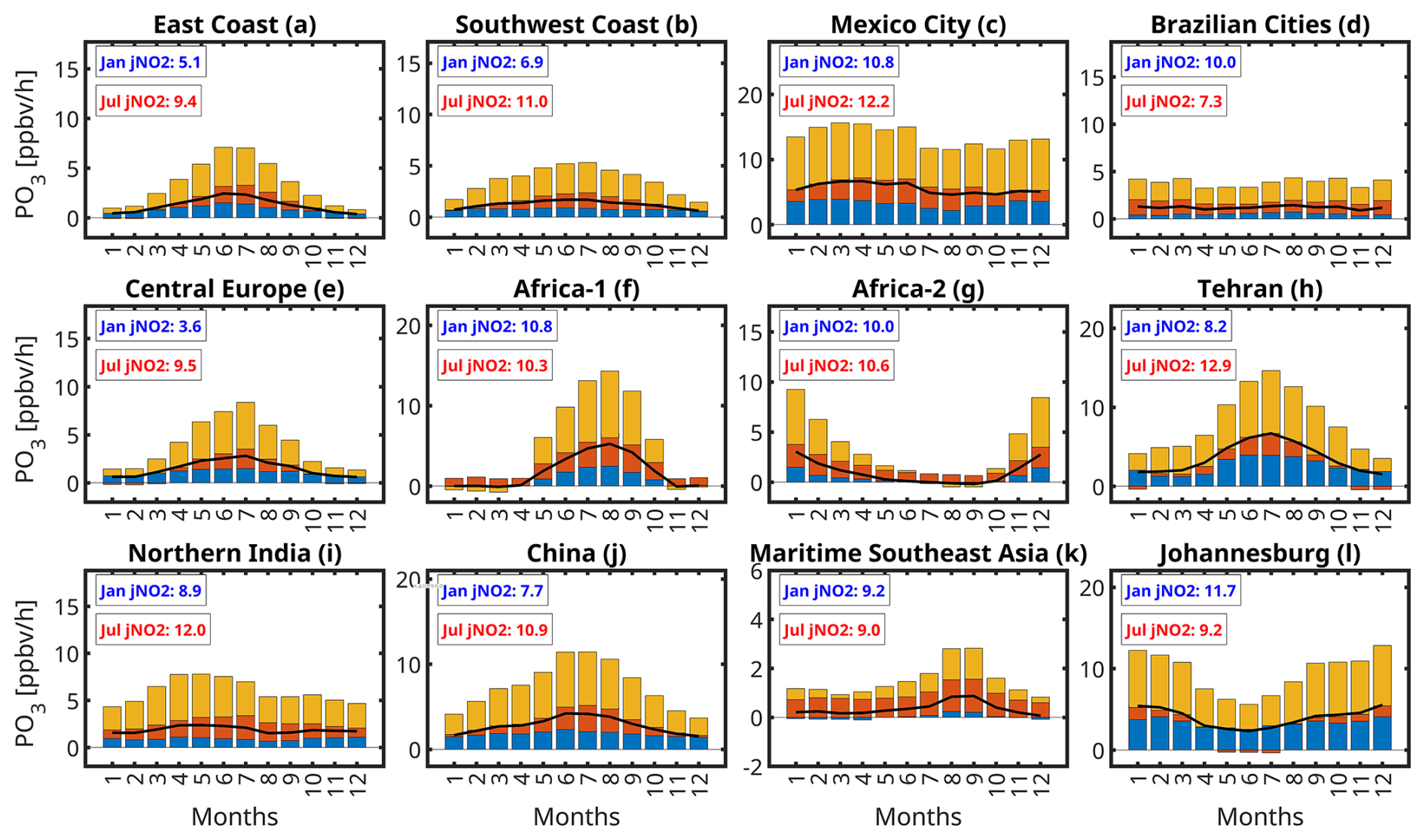
Figure 7 The bar plots of the sensitivity of PO₃ to photolysis rates (yellow bar), NO₂ (red bar), and HCHO (blue bar) concentrations within the PBL over the selected regions shown in Fig. 6. These sensitivities are influenced by both the magnitude of the precursors and the first-order derivative of PO₃ to the precursor, detailed in Appendix A. jNO₂ values are in 1 × 10⁻³ s⁻¹ units.

The amplitude of photolysis rates dictates the amplitude of the sensitivity of PO₃ to NO₂ and HCHO. For instance, over East Coast, Central Europe, and Tehran, the first derivative of PO₃ to NO₂ tends to be small during colder months, primarily because of reduced photochemistry. As a result, despite significantly higher NO₂ concentrations in these months, the sensitivity of PO₃ to NO₂ is muted. Conversely, in warmer months, the larger positive derivative of PO₃ relative to NO₂, driven by increased HCHO levels (shifting away from VOC-sensitive regimes) and enhanced photolysis rates, markedly increases the contributions of low summer NO₂ levels to PO₃. Likewise, we observe substantially higher sensitivity of PO₃ to HCHO concentrations during warmer seasons. This increase is attributed to both the elevated levels of HCHO and the growing derivative of PO₃ with respect to HCHO, both of which are directly influenced by enhanced photochemistry. One might argue that summer conditions should lead to a shift towards extremely NO_x-sensitive regimes, resulting in a reduced first-order derivative of PO₃ to HCHO. However, most polluted regions chosen for this figure are in transitional regimes during the summer, which renders PO₃ fairly responsive to HCHO concentrations.

The sensitivity of PO₃ to photolysis rates is dependent on pollution levels, just as its sensitivity to HCHO and NO₂ concentrations is influenced by photolysis rates. This is primary reason for seeing minimal seasonality of PO₃ over Mexico City, various Brazilian cities, and northern India. These minimal changes in photolysis rate sensitivities are caused by the less pronounced seasonality in both photolysis rates and pollution levels compared to other areas (Fig. S14). Souri et al. (2025) found that photolysis rates significantly contribute to the production of PO₃ when there is an adequate amount of ozone precursors. This was reflected in larger (smaller) coefficients associated with photolysis rates in PO₃LASSO algorithm for polluted (pristine) regions. For example, high photolysis rates over the Sahara do not significantly contribute to PO₃ because of the limited availability of ozone precursors needed to initiate the RO_x–HO_x cycle. A notable example can be observed in Africa, where photolysis rates tend to remain consistently high throughout the year under near cloud-free conditions (Fig. S14). However, there is a marked seasonality in the sensitivity of PO₃ with respect to photolysis rates during polluted months suggesting that the ample precursors can leverage available lights to form more ozone molecules. This pattern underscores the algorithm's capability to understand the intertwined relationships between the photolysis rate sensitivities and pollution levels, as well as the pollution sensitivities and photolysis rates.

4.4.3 Global PO₃ linear trends using OMI (2005–2019)

Using the linear trend calculation method outlined by Souri et al. (2024), we compute global long-term linear trends of PO₃ from OMI data, shown in Fig. 8. High-latitude regions (> 65°) are excluded due to limited photochemical activity. We observe large variability in both the signs and magnitudes of the linear trends. Predominantly positive trends occur over the Middle East, India, and China, while negative trends are mostly found in the eastern U.S., southern parts of Europe, maritime Southeast Asia, and several areas in Africa. The largest upward trend in PO₃ over the U.S. occurs in oil and gas producing regions, including the Permian Basin. While various physicochemical processes beyond near-surface PO₃ influence tropospheric ozone trends, the strong agreement between predominantly upward PO₃ trends in Asia and the Middle East suggested by satellite-based ozone observations (Gaudel et al., 2018; Boynard et al., 2025) is noteworthy.

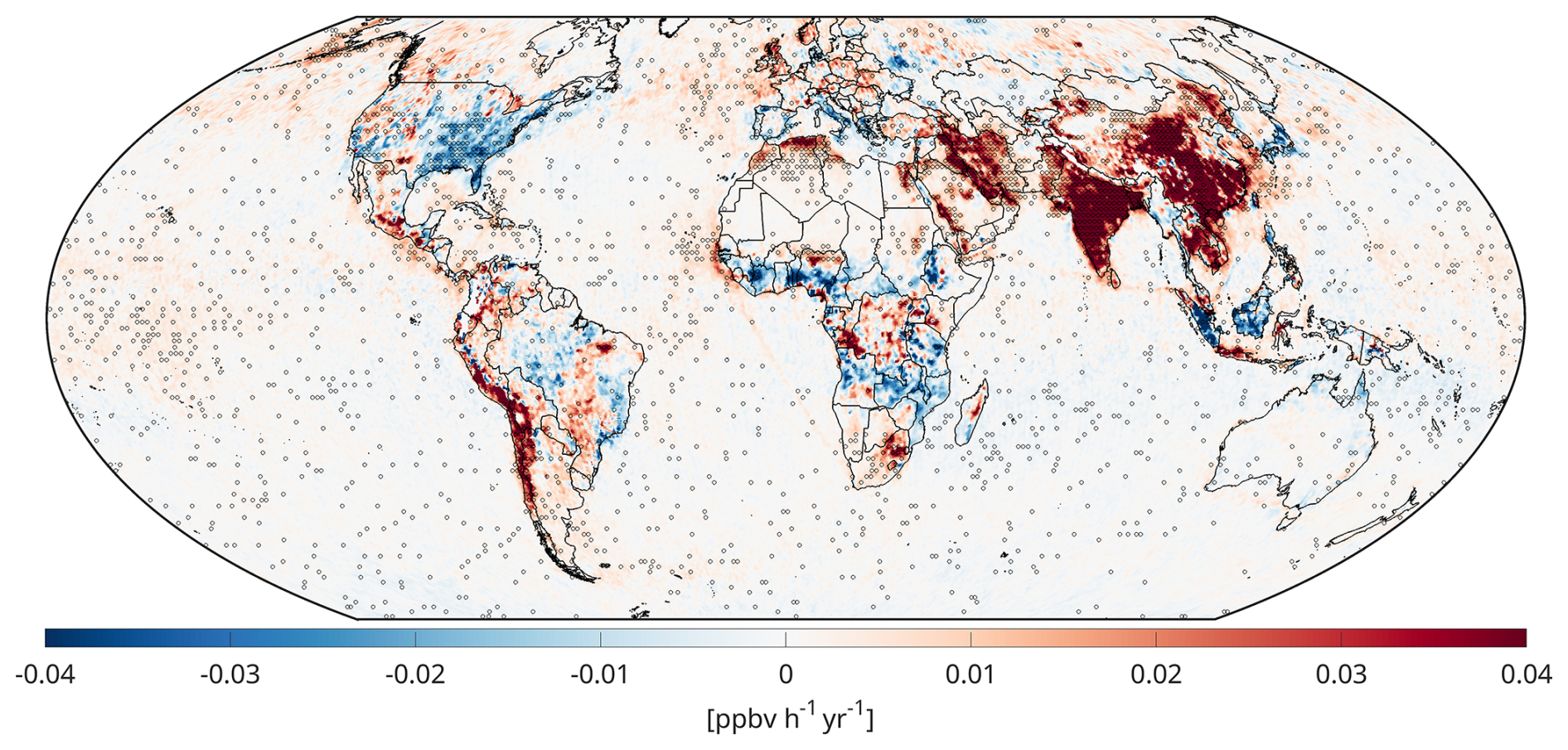
Figure 8 The linear trend maps of PO₃ within PBL derived from our new algorithm using OMI in 2005–2019. Dots indicate that the trend has passed a statistical test based on the Mann–Kendall test at 95 % confidence interval.

To gather a more relative perspective, Fig. 9 shows relative PO₃ trends (as percentages relative to 2005 annual averages) for regions where PO₃ exceeds 0.5 ppbv h⁻¹. The largest relative changes (> 30 %) are evident over the Persian Gulf, Chile, India, and China. Large negative values dominate over the eastern U.S. and over the central Africa (> 20 %).

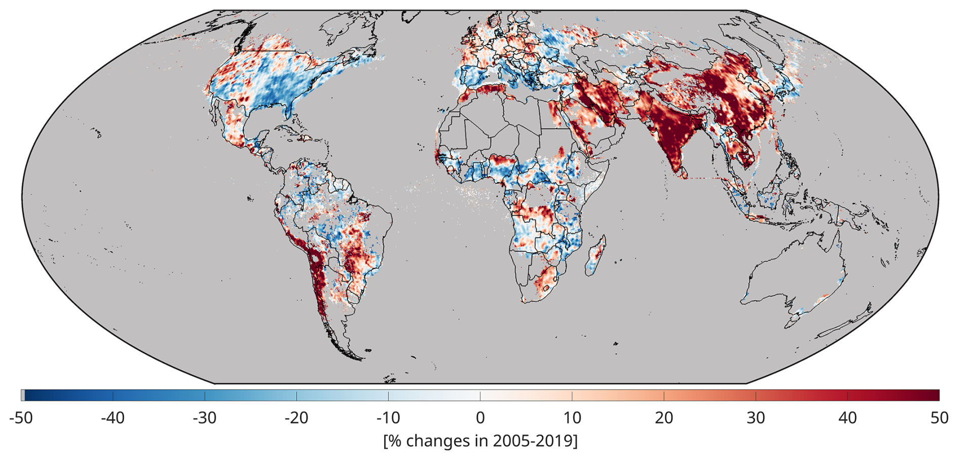
Figure 9 Similar to Fig. 8 but percentage changes are instead shown over PO₃ > 0.5 ppbv h⁻¹.

Multiple factors in our parameterization can simultaneously influence these trends, including changes in HCHO VCDs, NO₂ VCDs, dynamic changes in column-to-PBL conversion factors from MINDS, water vapor, and photolysis rates. However, photolysis rate trends should be negligible because long-term changes in total overhead ozone are insignificant at midlatitudes (Fig. S2 in Souri et al., 2024), and surface albedo is based on a monthly climatology dataset. While water vapor increases over time in response to global warming (Souri et al., 2024; Borger et al., 2022), these changes are insufficient to explain the large variability in PO₃ linear trends over polluted regions. Accordingly, simultaneous changes in HCHO and NO₂ boundary layer mixing ratios are the main drivers of PO₃ trends.

The PO₃ trends are generally explained by changes in ozone precursor concentrations which are mapped in Figs. S15 and S16. The attribution of trends in OMI HCHO and NO₂ have been partly discussed in Souri et al. (2024) and the references therein. Increases in both HCHO and NO₂ over the Middle East, India, and China drive rising PO₃ over time. Conversely, reduced HCHO and NO₂ concentrations over parts of Africa, the eastern U.S., and maritime Southeast Asia, have led to PO₃ reductions. However, many localized areas exhibit strong non-linearity. For instance, Tehran (Iran) shows positive PO₃ trends caused by NO₂ increases in a predominantly VOC-sensitive regime, reducing ozone loss through NO₂+ OH reactions. Los Angeles (USA) shows upward trends attributed to rapid NO₂ reductions, resulting in the opposite effect (Sect. S2)

The quantitative characterization of these trends (similar to our analysis of PO₃ seasonality in Sect. 4.4.2 or rapid PO₃ changes during a heatwave in Sect. S3) presents significant challenges for several reasons: (i) the amplitudes of these trends are generally an order of magnitude smaller than seasonal changes, requiring more stringent attribution methods, (ii) the sensitivities of PO₃ to input parameterization can behave non-linearly, making a linear trend analysis ill-suited for some localized areas, and (iii) changes in ozone precursors have effects on the sensitivity of PO₃ to photolysis rates as described in Sect. 4.4.2, introducing a convoluted problem.

Since our PO₃ parameterization encapsulates non-linear and interdependent relationships between pollution levels, light intensity, and water vapor, fully isolating individual effects on PO₃ trends requires reproducing the product while holding either NO₂ or HCHO constant individually and allowing others to evolve over time (an approach similar to modeling experiments in Souri et al., 2024). This approach comprehensively captures the non-linear dependencies between input variables and PO₃, circumventing the need for crude linear approximations.

4.4.4 High resolution TROPOMI-based PO₃ maps contrasted with OMI in 2019

Accelerated rates of PO₃ at approximately 13:30 LST are observed consistently across polluted midlatitude regions characterized by high photolysis rates. This pattern is substantiated by the global PO₃ maps derived from TROPOMI and OMI data for the year 2019 illustrated in Fig. 10. While the maps presented are averages for 2019, significant PO₃ hotspots (exceeding 8 ppbv h⁻¹) are identified over metropolitan/industrial areas including Mexico City (Mexico), Tehran (Iran), the Persian Gulf, and Hunan Province (China). There are less documented regions undergoing elevated locally-produced ozone such as Johannesburg (South Africa), Rio de Janeiro (Brazil), Sao Paulo (Brazil), and Santiago (Chile). In contrast, Europe emerges as a region with comparatively low PO₃ levels despite its dense population. This tendency may be attributed to lower photolysis rates (characterized by high solar zenith angles and low surface reflectivity) as well as effective emissions mitigation strategies. A notable similarity exists between these identified hotspots and those reported by Souri et al. (2025), although the contrast between clean and polluted areas is more pronounced in the PO₃DNN product because of an improved representation of PO₃DNN in clean regions.

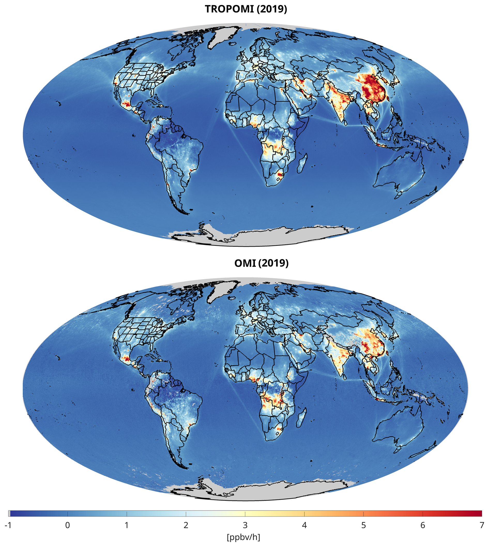
Figure 10 Global maps of PO₃ derived from TROPOMI (top) and OMI (bottom) datasets based on the PO₃DNN algorithm in 2019. These values are estimated within the PBL region at ∼ 13:30 LST. The data exclude cloudy pixels, strong smoke, sensor anomalies, and snow based on the recommended quality flags coming with TROPOMI and OMI products.

PO₃ exhibits a slight negative value over oceanic and densely forested areas (such as the Amazon and Congo), primarily because of ozone sinks associated with water vapor (H₂O(v)) and alkenes, which are implicitly included in our parametrization. However, a marked contrast is observed between the slightly negative and positive PO₃ levels along marine vessel pathways. These ship paths are informed not only by remote sensing data (Georgoulias et al., 2020) but also by the conversion of column measurements to PBL mixing ratios thorough the MINDS simulation, which accounts for ship emissions. Given that the PBL is typically shallow over marine regions, the conversion factor is expected to be substantial for these pathways, resulting in a pronounced contrast in pollution levels.

The finer spatial resolution of the TROPOMI dataset enhances the detail of the PO₃ maps compared to those derived from OMI, yielding less noise and fuller data. This reduction in gaps in TROPOMI-based PO₃ is attributed to a lower likelihood of cloud contamination and the full coverage of all pixels in the detector, in contrast to OMI, which suffers from the row anomaly. Visual analysis of the two datasets indicates that TROPOMI often shows higher PO₃ than OMI over polluted regions. Except for NO₂ and HCHO VCDs, the inputs to the parametrization are identical across both products.

To further investigate these differences, we synchronize the TROPOMI datasets at the OMI-based spatial resolution and produced scatterplots, as displayed in Fig. 11. The correspondence between the two products is high (R²= 0.86). Nonetheless, TROPOMI-based PO₃ levels are approximately 10 % greater than those derived from OMI. The fact that we observe this overestimation given that TROPOMI has been coarsened to match OMI's footprint suggests that the differing spatial resolutions (0.25° vs. 0.1°) are unlikely to account for the discrepancy. Moreover, we undertake a comparative analysis of NO₂ and HCHO mixing ratios within the PBL region as obtained from MINDS alongside these two satellite datasets. Given that the conversion factor remains consistent between the two products, any observed differences can be attributed to variations in their respective VCDs. Our analysis reveals that both NO₂ and HCHO mixing ratios are higher in TROPOMI relative to OMI (by 5 %–6 %), thereby providing a good explanation for higher TROPOMI-based PO₃ in comparison to OMI.

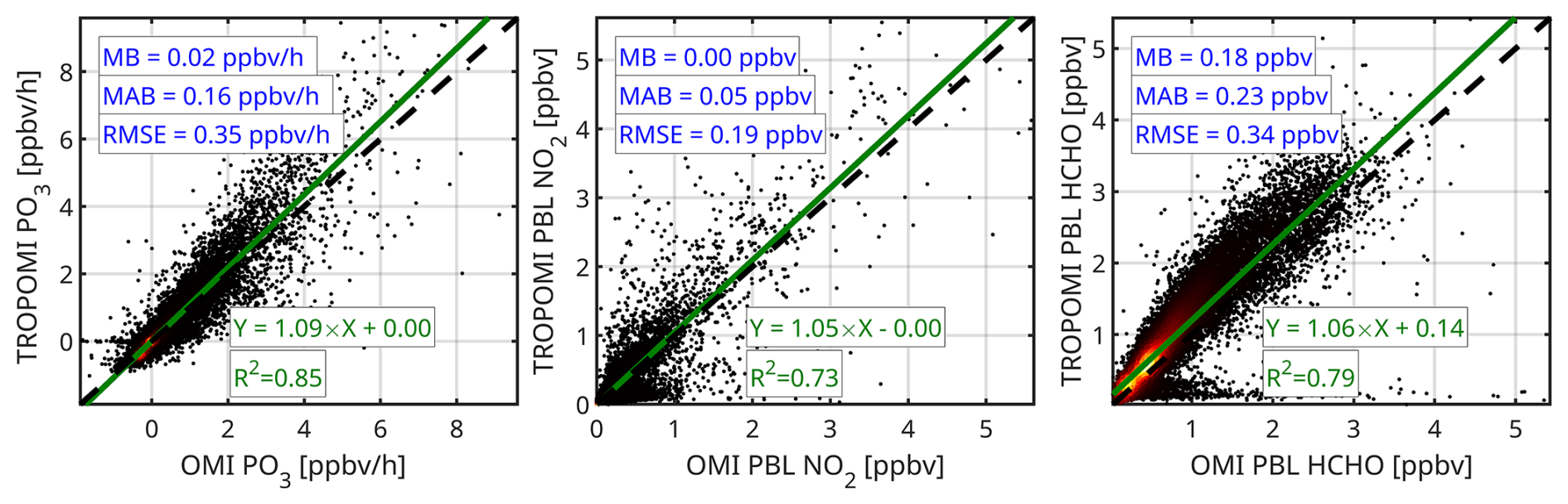
Figure 11 Scatterplots of (left) OMI PO₃ vs. TROPOMI PO₃, (middle) OMI PBL NO₂ vs. TROPOMI PBL NO₂, and (right) OMI PBL HCHO vs. TROPOMI PBL HCHO based on 2019. We coarsen TROPOMI dataset to match OMI's spatial resolution to remove the effect of spatial footprint on these results.

4.4.5 Error Analysis

Based on the formulation outlined in Sect. 3.4, we evaluate both the systematic and random error components of PO₃ for July 2019, based on data from both OMI and TROPOMI retrievals. Figure 12 presents the average error values for the month. Total PO₃ errors range from 25 % to 80 % in areas characterized by moderate to extreme pollution, while in more remote regions, errors can surpass 200 %.

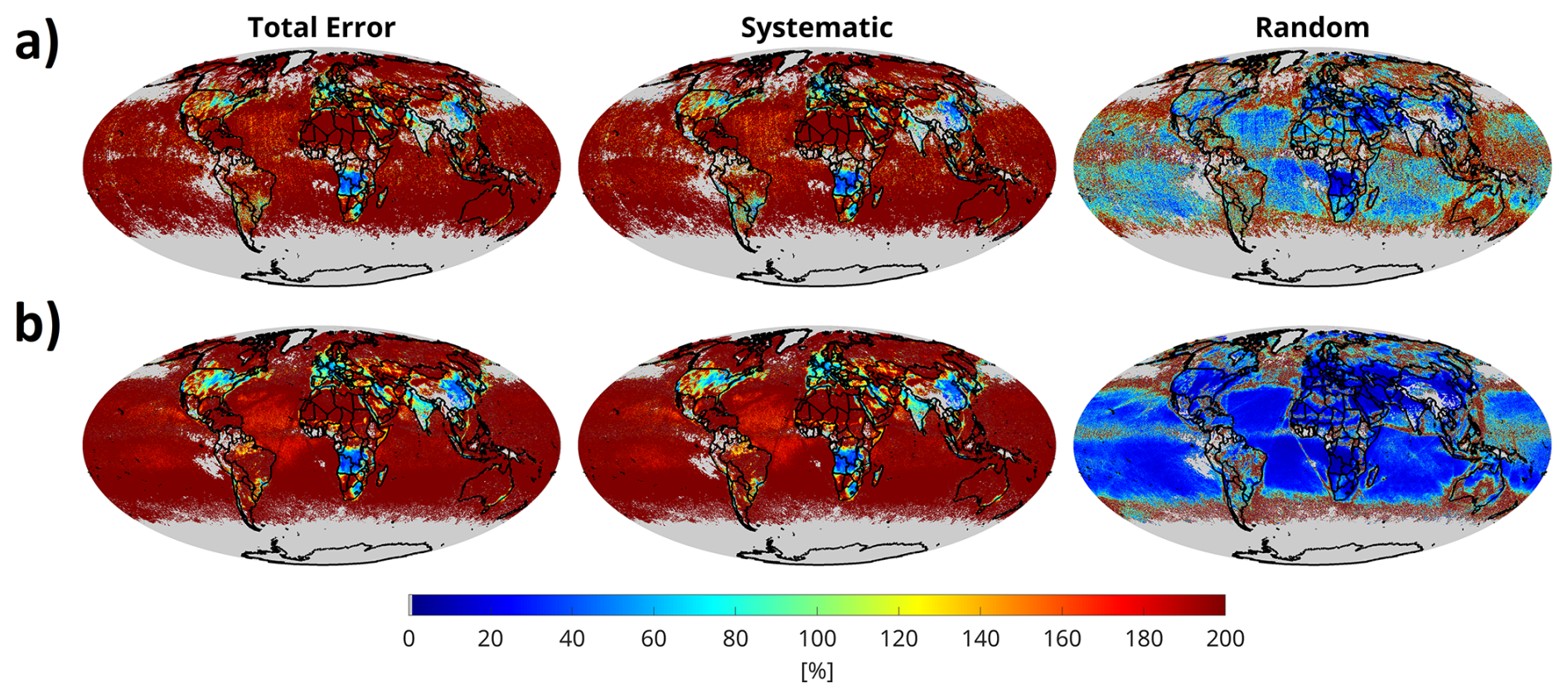
Figure 12 The maps of total error, systematic, and random errors for (a) OMI, and (b) TROPOMI computed for July 2019.

On average, random errors constitute only a small fraction of the total error budget, with OMI showing consistently larger random errors than TROPOMI across the region. This is primarily a result of OMI's limited sampling caused by row anomaly issues. As mentioned in Sect. 4.2, these random errors are significantly lower when compared to the PO₃LASSO random errors (Souri et al., 2025).

Systematic errors account for most of the total error, exceeding 90 %. These systematic errors are comprised of three components: biases arising from the correction of VCDs using ground-based remote sensing data, errors related to DNN predictions, and conversion factors derived from the MINDS framework. The first two components contribute minimally to the overall error (less than 5 %), making the MINDS conversion factors the dominant contributor to the total error budget. Therefore, any parametrization aimed at converting satellite-based VCDs to near-surface concentrations, including the one presented in this study, should always seek out a model that accurately reflects the shape of the profiles.

We also quantify the impact of inconsistent shape factors used in the retrievals and the MINDS profile on PO₃ estimates and find them introducing systematic errors of 5 %–25 % over PO₃>0.5 ppbv h⁻¹ (Figs. S17–S20). Refining TROPOMI and OMI products with MINDS shape factors would require reproducing several large-scale validation efforts (e.g., Verhoelst et al., 2021; Vigouroux et al., 2020; Pinardi et al., 2020; Ayazpour et al., 2025), which is beyond the practical scope and resources of this study.

4.4.6 Beyond binary maps obtained from FNR: Ozone sensitivity maps using high-resolution TROPOMI data

We explore the spatially varying sensitivity of PO₃ to HCHO and NO₂ worldwide using TROPOMI. These maps provide finer information compared to binary maps obtained from FNRs. Figure 13 illustrates global maps of these sensitivities averaged for the year 2019. We observe negative sensitivity values of PO₃ to NO₂ in urban areas, which aligns with our understanding of non-linear ozone chemistry. These negative values are particularly pronounced in northern China, where $\mathrm{VOCR}/{\mathrm{NO}}_x$ ratios remain low throughout the year. Similar non-linear feedback patterns can be seen in the Benelux region and the United Kingdom, primarily driven by elevated NO₂ levels. In contrast, NO₂ significantly contributes to higher PO₃ in southern China, India, Mexico, and several regions across Africa.

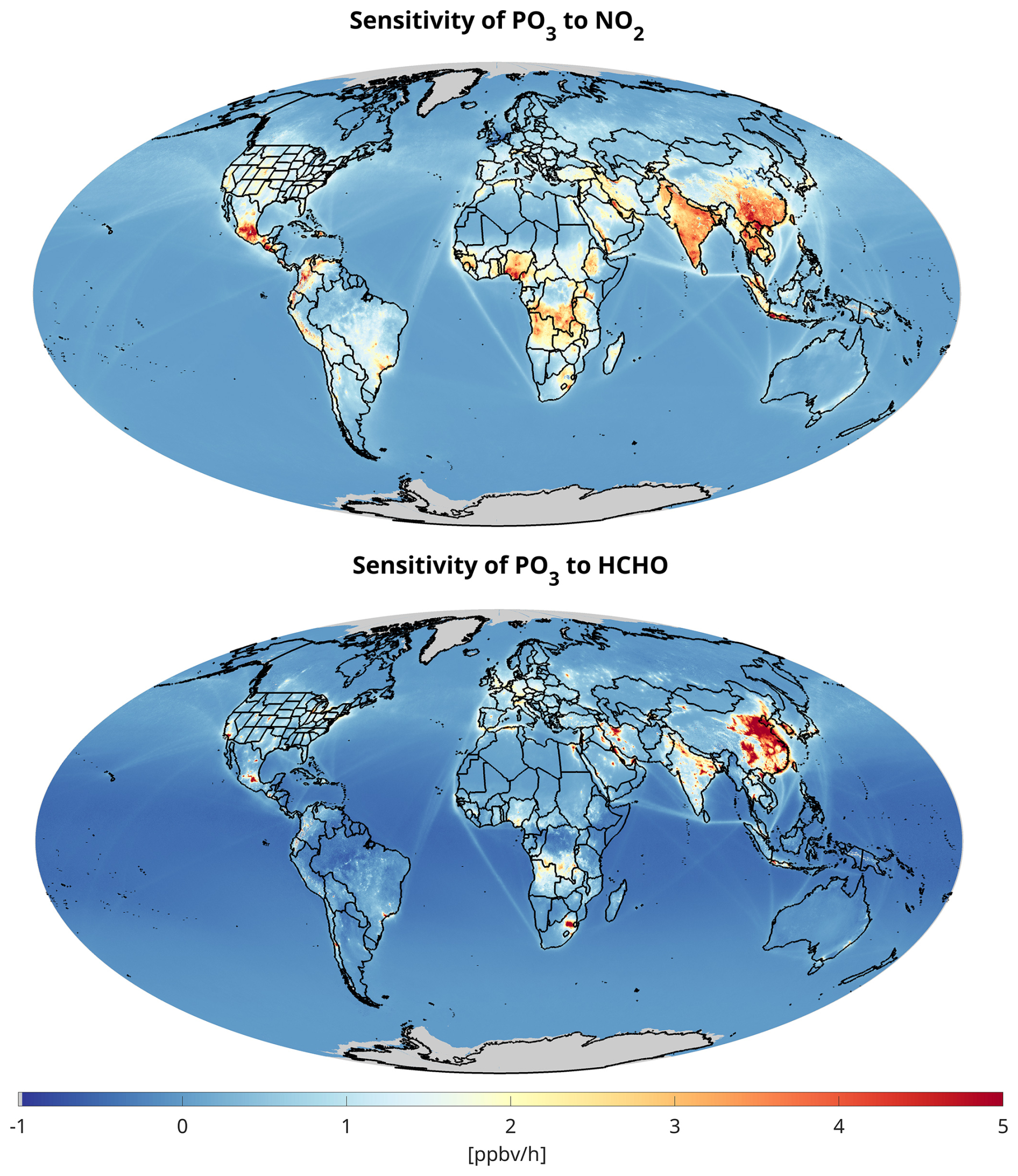
Figure 13 The sensitivity of PO₃ to NO₂ (top) and HCHO (bottom) based on our algorithm using TROPOMI data in 2019.

As indicated in Souri et al. (2025), the influence of HCHO on PO₃ is largely governed by NO_x emissions. This relationship explains why the sensitivity of PO₃ to HCHO closely mirrors global NO₂ levels, which dictates the locations of VOC-sensitive regimes. We observe slightly negative sensitivity of PO₃ to HCHO in remote and densely vegetated regions, likely a result of the effects of alkenes on ozone. However, the implicit nature of DNN makes it challenging to identify the exact chemical reasons behind these patterns. Noteworthy examples of areas where PO₃ is significantly influenced by HCHO include eastern China, Los Angeles (USA), Tehran (Iran), Mexico City (Mexico), and Johannesburg (South Africa).

Figure 14 presents the maps of PO₃ along with sensitivities across four seasons in 2019 over Middle East, derived from TROPOMI data. Notably, PO₃ values surge during the summer months in several densely populated and industrial regions of the Middle East. Furthermore, we observe considerable PO₃ values in the fall, primarily caused by the influence of HCHO. This fall peak is consistent with the observations made by Souri et al. (2025), who reported a sharp rise in PO₃ in late fall 2019 over Tehran (Iran). The overall seasonality of PO₃ is well aligned with the discussions presented in Sect. 4.4.1. The sensitivity of PO₃ to NO₂ exhibits notable variation, shifting from low and negative values during the colder months to positive and high values in the warmer months. We identify HCHO as the predominant contributor to PO₃ in these regions, as the majority of these cities fall in VOC-sensitive environments and emit significant amounts of anthropogenic HCHO, whether from primary or secondary sources.

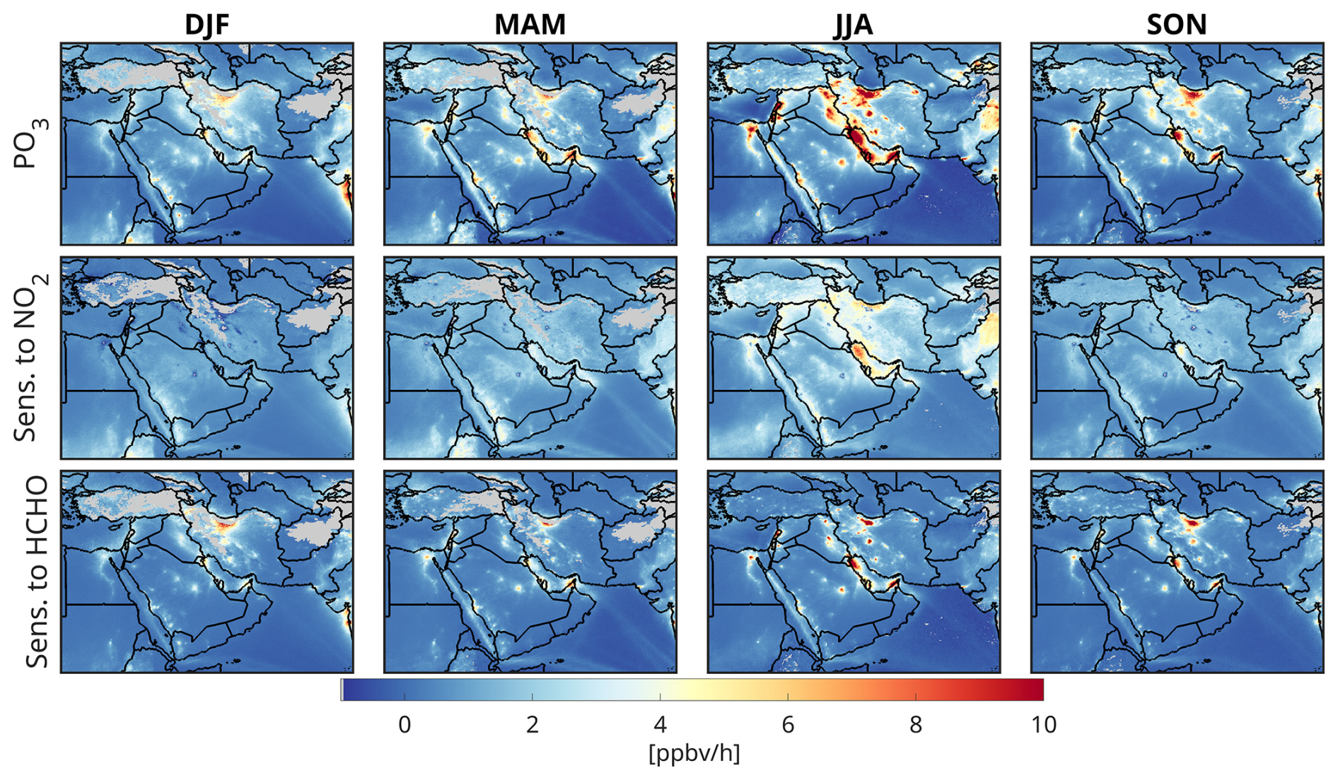
Figure 14 The magnitude of PO₃ and the corresponding sensitivity to NO₂ and HCHO over Middle East grouped into four different seasons. DJF: December-January-February, MAM: March-April-May, JJA: June-July-August, and SON: September-October-November. Sens. means sensitivity.

These maps eliminate the need for binarization of chemical conditions, as they effectively illustrate the spatial variability in ozone response to HCHO and NO₂ while accounting for light and humidity, two important dimensions missing in FNR-based ozone sensitivity diagnosis. A more detailed discussion about FNR's inability to fully describe ozone chemistry is documented in Sect. S1.

5 Summary

Early data-driven analyses of ozone chemistry sensitivity primarily relied on “ratio-based” indicators to partially linearize the non-linear aspects of urban ozone chemistry, which are influenced by pollution levels, light, and water vapor. With the development of more sophisticated algorithms, including machine learning techniques capable of fitting high-dimensional non-linear functions, we have shown that a highly effective parameterization of net ozone production rates (PO₃) can be achieved. This approach not only eliminates the need for empirical linearization of ozone chemistry through various indicators, but it also allows for the primary inputs to be accurately constrained using satellite observations. This advancement allowed us to move beyond the previously employed formaldehyde-to-nitrogen dioxide ratio (FNR) and to generate more comprehensive sensitivity maps, which account for variations not only in HCHO and NO₂ but also in light and water vapor.

We significantly enhanced the empirical parametrization of PO₃ described in Souri et al. (2025), in several key ways: (i) we improved the representation of PO₃ in both polluted and clean areas using a L2-regularized deep neural network (DNN) and eliminated the need for empirical linearization of atmospheric conditions with the FNR approach, resulting in reduced complexity and noise in the final estimates; (ii) we used a finer, up-to-date global transport model called MINDS to convert satellite-retrieved vertical column density (VCD) into planetary boundary layer (PBL) mixing ratios; (iii) we incorporated the error from these conversion factors, derived from comprehensive validation against aircraft spirals, into the total error budget; and (iv) we generated long-term records of PO₃ magnitudes and sensitivities to nitrogen dioxide (NO₂) and formaldehyde (HCHO) using bias-corrected data from the Ozone Monitoring Instrument (OMI) for the years 2005–2019 (at a resolution of 0.25° × 0.25°) and the TROPOspheric Monitoring Instrument (TROPOMI) for 2018–2023 (at a resolution of 0.1° × 0.1°). These datasets were collected under partially cloud-free conditions around 13:30 equatorial local standard time. The two products show strong agreement, with TROPOMI-based PO₃ being approximately 10 % higher than OMI, which is attributed to higher NO₂ and HCHO concentrations noted by TROPOMI.

The DNN algorithm (PO₃DNN) accounted for more than 96 % of the variance in both the test and training datasets derived from observationally-constrained box simulations across various atmospheric composition campaigns, with a slope close to the unity line. The new algorithm improved the representation of PO₃ in remote regions compared to the version developed in Souri et al. (2025), due to the inclusion of water vapor and the use of a more robust regression model. We found PO₃DNN to be logically responsive to its inputs during various idealized experiments that involved changing light conditions, pollution levels, and water vapor.

Expectedly, our results indicate that PO₃ magnitudes and sensitivity maps are primarily influenced by the levels of ozone precursors, non-linearity of ozone chemistry, and photolysis rates. We revisited the accelerated PO₃ observed in Souri et al. (2025) across polluted areas, such as major cities and during biomass burning activities in photochemically active environments. Using sensitivity calculations derived from the new algorithm, we investigated the contributors to PO₃ seasonality around the globe. We found that photolysis rates were the primary drivers of PO₃ seasonality. During darker months, both the magnitude of PO₃ and its sensitivity to NO₂ and HCHO decrease due to limited light availability to initiate the RO_x–HO_x cycle. This critical trend is not represented by the pollution levels alone, highlighting the necessity of including photolysis rates in ozone sensitivity analyses. Fortunately, we can largely constrain these rates using satellite observations. In regions with minimal variability in photolysis rates (such as the tropics), pollution levels became the main driver of PO₃ seasonality.

The long record of stable observations from OMI allowed us to generate the first-ever maps of PO₃ linear trends from 2005 to 2019 globally. The global long-term trends revealed substantial spatial variability, with predominantly positive trends over Asia and the Middle East (> 30 % relative to 2005) and negative trends across the eastern U.S., Europe, and parts of Africa. Analysis indicated that simultaneous changes in HCHO and NO₂ boundary layer concentrations were the primary drivers of these trends. Although increases in both precursors over Asia and the Middle East, rising PO₃ and reduced concentrations elsewhere lead to PO₃ decreases, localized non-linearities complicated this relationship, as demonstrated by contrasting chemical regimes in Tehran vs. Los Angeles. Quantitative attribution of these trends presents challenges because of their small amplitudes relative to seasonal variations and non-linear sensitivities in the parameterization, necessitating “hold-one-out” approaches that account for complex interdependencies between input variables.

We error characterized both systematic and random errors associated with PO₃DNN for both OMI and TROPOMI-based products. We showed that total errors range from 25 % to over 200 %, with smaller errors in polluted areas. Random errors are minor on monthly-basis, with OMI exhibiting larger errors due to row anomaly issues. Systematic errors exceed 90 % of the total error, primarily driven by MINDS conversion factors. The total errors budget emphasizes on the role of model used for converting satellite-based VCDs to near-surface concentrations and its importance for precisely determining ozone precursors levels near to the surface. Furthermore, in future efforts, we also need to refine satellite retrievals using spatially higher-resolution AMFs derived from MINDS while simultaneously performing retrieval validation against ground-based remote sensing observations.

We developed a novel product aimed at enhancing our understanding of the variability in PO₃ and its interactions with NO_x and VOCs on a global scale. This advanced algorithm has undergone meticulous tuning and training using an extensive dataset derived from a reliable box model, which is further constrained by intensive atmospheric composition campaigns conducted by NASA and NOAA. The algorithm not only yields accurate estimates of PO₃ with minimal bias in comparison to observationally-constrained values but also facilitates the derivation of PO₃ in relation to HCHO and NO₂. However, as indicated by Souri et al. (2025), there remain several opportunities for further improvement, including: (i) the incorporation of heterogeneous chemistry; (ii) consideration of the impact of partially cloudy regions and aerosols on photolysis rates; (iii) gauging the potential benefits of using more sophisticated chemical mechanisms for the generation of the training dataset; and (iv) enhanced representation of vertical profiles of NO₂ and HCHO using observationally-constrained chemical transport models with more rigorous column to near-surface conversion methods (Cooper et al., 2020). Some of these enhancements present significant challenges, particularly the fine-resolution three-dimensional characterization of aerosol and cloud properties on a global scale, which is not obtainable with current reanalysis data. However, with the advent of newer satellite technologies such as PACE and MAIA, there may be opportunities to improve the representation of atmospheric models with respect to cloud and aerosol characteristics.

While the OMI- and TROPOMI-based PO₃ products maintain algorithmic consistency in several key components, including photolysis rates and water vapor calculations, the underlying satellite retrievals of HCHO and NO₂ VCDs remain unharmonized between the two instruments. To address the resulting inter-instrument biases, we implemented bias correction using ground-based remote sensing retrievals as reference standards. This approach achieved OMI and TROPOMI PO₃ agreement within 10 % on average. However, this level of consistency may be insufficient for robust joint trend analysis of the combined OMI-TROPOMI PO₃ record over areas with non-linear or minor trends, potentially requiring the implementation of trend harmonization algorithms (e.g., Hilboll et al., 2013) to ensure statistical reliability in long-term analyses.

The emergence of novel geosynchronous orbit (GEO) technologies is becoming increasingly important for monitoring the daylight hourly variability in ozone precursors. In particular, the finer spatial and temporal resolution offered by the Tropospheric Emissions: Monitoring of Pollution (TEMPO), Geostationary Environment Monitoring Spectrometer (GEMS), and Sentinel-4 instruments will aid in distinguishing exceptional events from typical atmospheric conditions. In light of the success of emission mitigation strategies over high income countries, the occurrences of elevated PO₃ are becoming more infrequent, thereby necessitating a more detailed and rapid observational strategy for monitoring such events. This presents a timely opportunity to address ozone exceedance events using TEMPO in conjunction with our PO₃ estimator, especially since the algorithm is designed to handle light-limited conditions – such as those encountered during early morning and late afternoon periods when TEMPO collects data – conditions that are not feasible to analyze via the FNR approach.

Appendix A: The sensitivity maps are the directional derivative

To demonstrate that the sensitivity calculation of PO₃ to its inputs resembles (Eq. 3) a directional derivative output, we can approximate the perturbations in the PO₃DNN (denoted as f(x), where x is the targeted sensitivity parameter) using the Taylor expansion:

$$\begin{array}{}\text{(A1)}& {\displaystyle }\begin{array}{rl}f\left(\mathrm{1.1}x\right)\approx f\left(x\right)& +\left(\mathrm{1.1}x-x\right)\mathrm{\nabla }f\left(x\right)\\ & =f\left(x\right)+\mathrm{0.1}x\mathrm{\nabla }f\left(x\right)\end{array}\text{(A2)}& {\displaystyle }\begin{array}{rl}f\left(\mathrm{0.9}x\right)\approx f\left(x\right)& +\left(\mathrm{0.9}x-x\right)\mathrm{\nabla }f\left(x\right)\\ & =f\left(x\right)-\mathrm{0.1}x\mathrm{\nabla }f\left(x\right)\end{array}\end{array}$$

The sensitivity calculation presented in Eq. (3) can be rewritten in the following form:

$$\begin{array}{}\text{(A3)}& \begin{array}{rl}S=& {\displaystyle \frac{(f\left(x\right)+\mathrm{0.1}\mathrm{\nabla }f\left(x\right))-(f\left(x\right)-\mathrm{0.1}\mathrm{\nabla }f\left(x\right))}{\mathrm{0.2}}}\\ & ={\displaystyle \frac{\mathrm{0.2}x\cdot \mathrm{\nabla }f\left(x\right)}{\mathrm{0.2}}}=x\mathrm{\nabla }f\left(x\right)\end{array}\end{array}$$

Therefore, the first-order approximation of the DNN prediction, when using the given sensitivity calculation, is x∇f(x) which represents the first-order Taylor expansion term that describes how the output changes with respect to both the gradient and the magnitude of x (i.e., directional derivative).

Appendix B: MINDS conversion factor validation

We validate the column conversion factors obtained from the MINDS simulations against corresponding values derived from aircraft spirals from several suborbital missions. The concentrations of HCHO and NO₂ in both datasets are collocated in time and space and are resampled onto a common vertical grid, ranging from the near surface up to 450 hPa in 20 hPa increments. To determine the conversion factors, these resampled concentrations are averaged within the PBL and then divided by the vertically integrated partial columns from the surface to 450 hPa. The PBLH is based on the MINDS simulations. Figure B1 displays scatterplots of the paired conversion factor binned at 12:15 and 15:15 LST (±45 min around the TROPOMI/OMI local revisit time) for NO₂ and HCHO, respectively. The unit for these conversion factors is ppbv col⁻¹, where col represents 1 × 10¹⁵ molec. cm⁻². The comparison shows a good level of agreement between the two datasets for both species (R²>0.7). The MINDS simulations perform slightly better for NO₂ than for HCHO. This performance difference may arise from the fact that HCHO is mainly a secondary product, meaning various uncertain VOC emissions, along with uncertain chemical processes in the model, could pile up leading to discrepancies in the vertical distribution of simulated HCHO compared to observations. Furthermore, HCHO vertical profiles can be easily affected by local circulation patterns that are difficult to resolve in coarse models (Souri et al., 2023b). We observe consistent model performance across various campaigns, except for DISCOVER-AQ Colorado. This discrepancy may result from complex topography and wind conditions in that region that the model might not fully capture. The differences between the two datasets can also be attributed to sources of error beyond the model deficiencies. For instance, the MINDS simulations represent a quarter-degree averaged concentration, which differs from the localized air samples derived from aircraft, known as the spatial representation error (Souri et al., 2022).

To account for the systematic errors resulting from the MINDS simulation in our error budget, we assign e_conv-HCHO and $e_{{\text{conv-NO}}_{\mathrm{2}}}$ in Eq. (5) to RMSE values obtained from the comparison. The choice of RMSE is based on the fact that it contains information about the bias and the dispersion of MINDS with respect to the observations. We assume these errors to be invariant by time or location, mainly because of limited aircraft spirals (N= 57) we have from the suborbital missions.

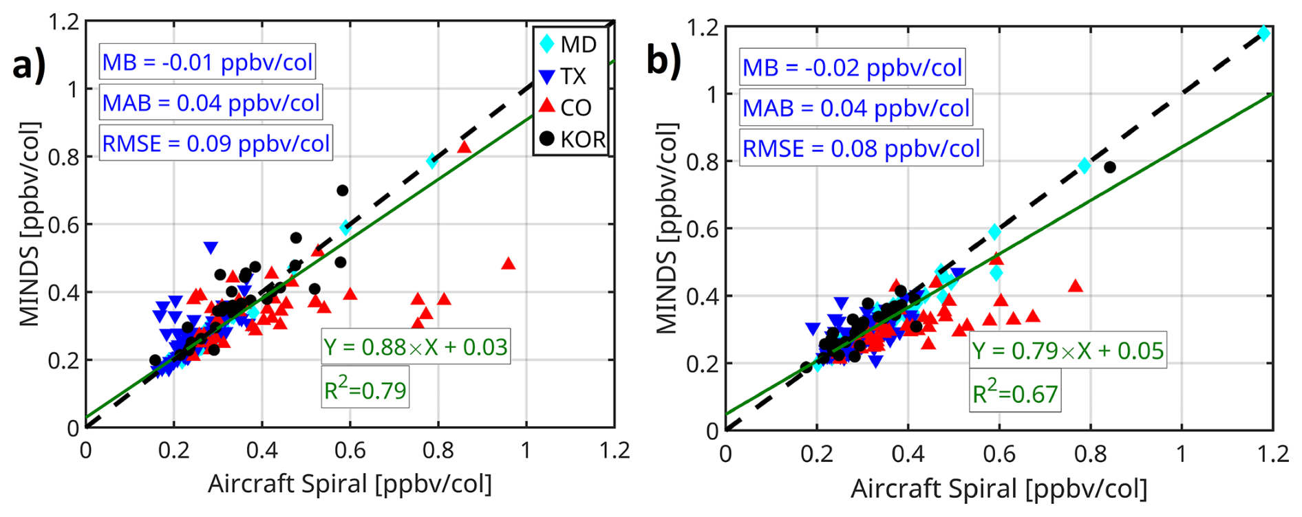
Figure B1 The scatterplot of the column to the PBL conversion factor for (a) NO₂ and (b) HCHO obtained from aircraft spirals (x axis) and MINDS simulation (y axis) at the same time and location from four different suborbital missions. These 57 spirals are limited to OMI/TROPOMI overpass ±45 min buffering time. “col” denotes 1 × 10¹⁵ molec. cm⁻².