the Creative Commons Attribution 4.0 License.
the Creative Commons Attribution 4.0 License.
 | 11 Jun 2026
Detection of ozone recovery in the Arctic from ground-based measurements
Caroline Jonas
Corinne Vigouroux
Bavo Langerock
Robin Björklund
Anne Boynard
Thomas Carlund
Martine De Mazière
Peter Effertz
Quentin Errera
Matthias M. Frey
José Granville
James W. Hannigan
Arno Keppens
Nis Jepsen
Rigel Kivi
Norrie Lyall
Mathias Palm
Maxime Prignon
Viktoria F. Sofieva
Kimberly Strong
Tove Svendby
David Tarasick
Laura Thölix
Roeland Van Malderen
Yana Virolainen
Sibylle von Löwis
Xiaoyi Zhao
Contrary to the Antarctic, where ozone recovery has been observed for about a decade, the detection of positive ozone trends in the Arctic remains challenging due to higher natural variability of ozone in that region.
Using a merging of long-term ozone data from Fourier transform infrared spectrometers, ozonesondes, and Dobson and Brewer spectrophotometers, we present regional long-term trends (2000–2024) for total, stratospheric and tropospheric ozone. First, ground-based measurements are cross-compared to two satellite data sets (MEGRIDOP and IASI-CDR). This enables the detection of drifts in ground-based data sets we further exclude from our study. We then use a representativeness study based on CAMS re-analysis data to define regions for which representative trends with reduced uncertainties are obtained by combining data sets from different instruments and stations. Annual and seasonal trends are calculated using a multiple linear regression technique involving a set of proxies that represent physical processes influencing the natural ozone variability.
Annual trends indicate increasing total ozone over the Arctic, and are statistically significant over Canada and Reykjavik (+2.1 % per decade) and North-West Europe (Harestua and Lerwick, +0.7 % per decade). Ozone recovery is also observed over Canada in the mid-stratosphere (+2.0 % per decade) and over the North Pole region (Canada and Ny-Ålesund) in the upper stratosphere (+2.1 % per decade to +3.8 % per decade). By analyzing the sensitivity of the ozone trends to the proxies, we observe a slow down of the expected ozone recovery, especially in the lower stratosphere, due to stratospheric cooling (−0.6 % per decade) and to the increase of volume of polar stratospheric clouds (−0.8 % per decade).
- Article
(23847 KB) - Full-text XML
- BibTeX
- EndNote


Following the discovery of the Antarctic ozone hole (Farman et al., 1985) in the 1980s, the Montreal Protocol of 1987 (and its amendments) banned the production of chlorine-releasing chemicals such as chlorofluorocarbons that were found largely responsible for the global ozone depletion, earning them the name of ozone-depleting substances (ODS). Consequently, a progressive recovery of the ozone layer has been expected since the 2000s, with a projected complete recovery of stratospheric ozone around the 2050s globally (World Meteorological Organization, 2023). While this recovery has been established over Antarctica during the ozone hole onset period in September and in the mid-latitudes (at least for the total column of ozone near-global average 60° S–60° N), it remains elusive above the Arctic (Weber et al., 2022; World Meteorological Organization, 2023). First indications of recovery over the Arctic have been reported for the total column of ozone using ground-based and satellite measurements (Pazmiño et al., 2023; Bernet et al., 2023; Anjali and Kuttippurath, 2025), and in the upper stratosphere using satellite measurements (Arosio et al., 2019; Sofieva et al., 2021; Anjali and Kuttippurath, 2025). But the largest concentration of ozone in the atmosphere is located in the lower and middle stratosphere, at approximately 20 km of altitude. There, no recovery has yet been observed and instead, negative trends over the last two decades have been reported in the northern hemisphere (Ball et al., 2018; Nilsen et al., 2024). Model simulations suggest these negative trends could be due to the internal variability of ozone transport for northern mid-latitudes (Chipperfield et al., 2018; Benito-Barca et al., 2025), while in the Arctic, simulations suggest that stratospheric cooling induced by climate change implies large winter and spring losses of stratospheric ozone (von der Gathen et al., 2021). Ozone layer depletion as is common over Antarctica does occasionally occur over the Arctic as well – unlike at mid-latitudes – due to colder temperatures and the presence of polar stratospheric clouds. During springtime, when coldest temperatures ally with the first sunlight after the polar night, heterogeneous ozone-depleting reactions primarily occur on the surface of these clouds in the lower stratosphere. Compared to Antarctica, the detection of positive long-term ozone trends in the Arctic is much more difficult due to a larger natural variability of ozone (Brasseur and Solomon, 2005; Langematz and Tully, 2018) resulting from stratospheric dynamical activity, exemplified by the instability of the Arctic polar vortex (Jonassen et al., 2020). At the same time, expected stratospheric ozone trends in the Arctic are very small – a few percent per decade – complicating their detection over a noisy background.
In addition to stratospheric ozone, we also report on tropospheric ozone trends in the Arctic. Tropospheric ozone is a harmful pollutant with marked health impacts, important to monitor in its own right. But it is also necessary to study its impact on the total ozone column budget and separate it from stratospheric ozone trends. In Van Malderen et al. (2025a, b), significant negative tropospheric ozone trends were found in the Arctic for the 2000–2022 period of approximately −1 to −2 DU per decade, while Law et al. (2023) reported a strong seasonal cycle in tropospheric ozone trends, with a decrease during spring and increase during summer over the 1993–2019 period.
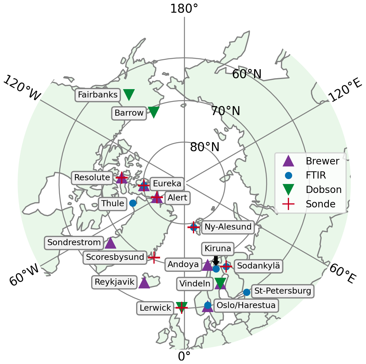
Figure 1Location of the 17 ground-based stations in the Arctic within 60–90° N considered in this study.
The aim of this study is to use different atmospheric ozone ground-based data sets over the Arctic to look for signals of recovery. We use data from 17 different stations, all located between 60 and 90° N (see Fig. 1) and from four different ground-based instrument techniques: Fourier transform infrared (FTIR) interferometers, ozonesondes, Brewer and Dobson spectrophotometers. Simultaneous use of these techniques enables to cover the whole stratosphere and troposphere: FTIR, Brewer and Dobson provide total columns of ozone, ozonesondes yield high-resolution profiles up to approximately 30 km, and four partial columns (one in the troposphere and three in the stratosphere) can additionally be extracted from FTIR. Each individual technique has been used in the past for trends detection (see e.g. Vigouroux et al., 2008, 2015 for FTIR, Kivi et al., 2007 and Christiansen et al., 2017 for ozonesondes and Harris et al., 1997 and Fioletov et al., 2023 for Brewer and Dobson).
The detection of stratospheric ozone trends typically requires the use of a multiple linear regression (MLR) in order to account for its variability, by explaining the time series variance by fitting several influencing physical processes. Those processes are typically the 11-year solar cycle, the Quasi-Biennal Oscillation (QBO) and the El-Niño Southern Oscillation (ENSO) as in the Long term Ozone Trends and Uncertainties (LOTUS) initiative (Petropavlovskikh et al., 2019). In the Arctic, the large ozone inter-annual variability is driven both by chemistry and by dynamics. Chemistry impacts ozone variability in polar regions through heterogeneous chemistry on polar stratospheric clouds (PSC). Dynamical variability is led by tropospheric planetary waves, which impact the stratospheric temperature and the Brewer-Dobson circulation (BDC) (Chipperfield and Santee, 2022), as well as by Arctic Oscillation (AO) which impacts the polar vortex (Lawrence et al., 2020) or by the equivalent latitude (EL) (Wohltmann et al., 2005). On a local scale, variability also depends on the tropopause pressure (TP) variations through stratosphere-troposphere exchanges. These processes are not independent, as e.g. the PSC formation is linked to the stratospheric temperature, and hence to the strength of the vortex. Various past studies used some of those drivers of polar ozone variability in multiple-linear regression (MLR) models (Vigouroux et al., 2015; Coldewey-Egbers et al., 2022; Weber et al., 2022; Bernet et al., 2023). A systematic statistical analysis of ozone proxies was carried out in Mäder et al. (2007) on ground-based data sets for the 1960–2000 period using a stepwise regression procedure. It concluded that in the North polar region, the optimized model includes the EL, PSC, Stratospheric temperature and aerosols. We do not consider aerosols here since in our period of focus there has been no major volcanic eruption in the North Hemisphere. To avoid biases due to pre-selection of proxies, in this work we also carry a stepwise regression procedure based on all proxies influencing ozone variability (11-year solar cycle, QBO, ENSO, PSC, EL, TP, Stratospheric temperature, BDC, and AO). The stepwise regression automatically selects the most significant proxies in the MLR and avoids overfitting. Overfitting is further controlled by verifying that the fitting is improved while the uncertainties of trends are reduced when adding new proxies. Some of these proxies have their own trend. Depending on the aim, one can choose to de-trend the proxies (as in e.g. Li et al., 2023), obtaining then an ozone linear trend that contains both influence of ODS and dynamics changes. We prefer here not to de-trend them, in order to obtain the ozone trend that would be due only to ODS changes, following e.g. Weber et al. (2022). Our trends can therefore be directly associated to the “recovery” of stratospheric ozone.
We further reduce the uncertainties of our trends by combining ground-based measurements into specific geographic regions, defined by performing a representativeness study (Weatherhead et al., 2017) based on the CAMS Re-Analysis data (Inness et al., 2019) for the total column of ozone and all four atmospheric layers, as done for tropospheric ozone in Van Malderen et al. (2025b). We thus obtain regional trends representative of these specific regions. We focus on the 2000–2024 period, since 2000 is commonly established as the onset of the ODS decline in the Arctic (World Meteorological Organization, 2023). The merging allows to include shorter time-period measurements or with gaps.
All data sets used are explicitly described in Sect. 2. In Sect. 3, we cross-compare ground-based data sets against two satellites ozone data sets, IASI-CDR (IASI, 2025) and MEGRIDOP (Sofieva et al., 2021). This enables us to validate the quality of our individual ground-based data sets before calculating trends, while also evaluating the drifts of satellite data sets with respect to ground-based instruments in the Arctic. The representativeness study and resulting regions for all total and partial columns are described in Sect. 4. Finally, we present in Sect. 5 our stepwise MLR model and the trends obtained in each of these regions for the four atmospheric layers (from 0 to 48 km) and for the total column of ozone.
All the ground-based data sets used in this work, their instrument's location, repository and time period are summarized in Table 2. The rest of this section describes all these data sets with more details, including a brief discussion of the measurement techniques and of the associated uncertainties.
2.1 FTIR interferometers
The FTIR interferometers record interferograms from sunlight that are Fourier-transformed into solar absorption spectra. Trace gas abundances, such as ozone abundances, are retrieved from these spectra by using line-by-line spectral fitting softwares (SFIT4, Hannigan et al., 2024, or PROFFIT, Hase et al., 2004), including radiative transfer models. Forward model inputs include spectroscopic parameters, climatological a priori information on trace gases concentrations, and 6-hourly pressure and temperature profile information from NCEP. The pressure and temperature-dependences of the ozone line-shapes enable us to retrieve low-vertical resolution profiles, with four to five distinct degrees of freedom for signal (DOFS), spanning the troposphere and stratosphere from approximately 0–48 km (Vigouroux et al., 2015).
In this study, we use FTIR ozone data sets from the Network for the Detection of Atmospheric Composition Change (NDACC) (https://ndacc.larc.nasa.gov/, last access: 8 June 2026). This network gathers the data sets of 160 ground-based instruments monitoring various components of the atmosphere from 73 active sites around the globe since 1990. This network enables detection of long-term trends, validation of other data sets and models (De Mazière et al., 2018). There are six NDACC FTIR instruments within the Arctic: Ny-Ålesund, Eureka, Kiruna, Harestua, St-Petersburg and Thule, see Table 2. These instruments are Bruker high-resolution (<0.005 cm−1) spectrometers. The retrieval strategy used at all these sites is standardized by the InfraRed Working Group (IRWG) (IRWG, 2025). It has been recently updated from the previous version described in details in Vigouroux et al. (2015) to an improved strategy (IRWG2023), based on the HITRAN2020 molecular spectroscopic database (Gordon et al., 2022), specific spectral microwindows (around 1000 cm−1) fitted to avoid interference with water vapor lines, an updated regularization scheme (Tikhonov) and an updated a priori (WACCMv7 IRWG, IRWG, 2025). More details on this new strategy used here can be found in the Appendix of Björklund et al. (2024), where it was shown to reduce biases with other instruments in Lauder, New Zealand from 1 %–3 % for all partial columns as well as to reduce drifts.
In addition, we consider a new ozone time series (Kivi et al., 2026) obtained by applying a new retrieval (in the 3040 cm−1 region following the strategy of Zhou et al. (2020) and García et al., 2014) to spectra recorded by the Sodankylä instrument that is part of the Total Carbon Column Observing Network (TCCON). The resulting vertical profiles contain lower DOFS of approximately 2.5, concentrated on the stratospheric layers, see Table 1.
Table 1Mean FTIR random, systematic and total uncertainties in percent and average degrees of freedom of signal (DOFS) of NDACC FTIR and of Sodankylä FTIR for each partial column and the total column of ozone (TCO).
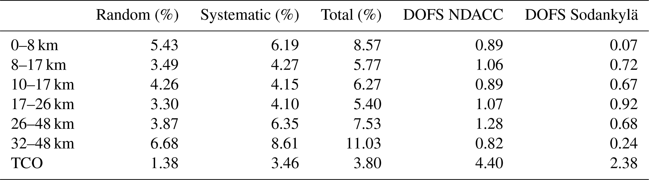
Table 2Summary of all the ground-based data sets that have been considered in this study ordered by decreasing latitude.
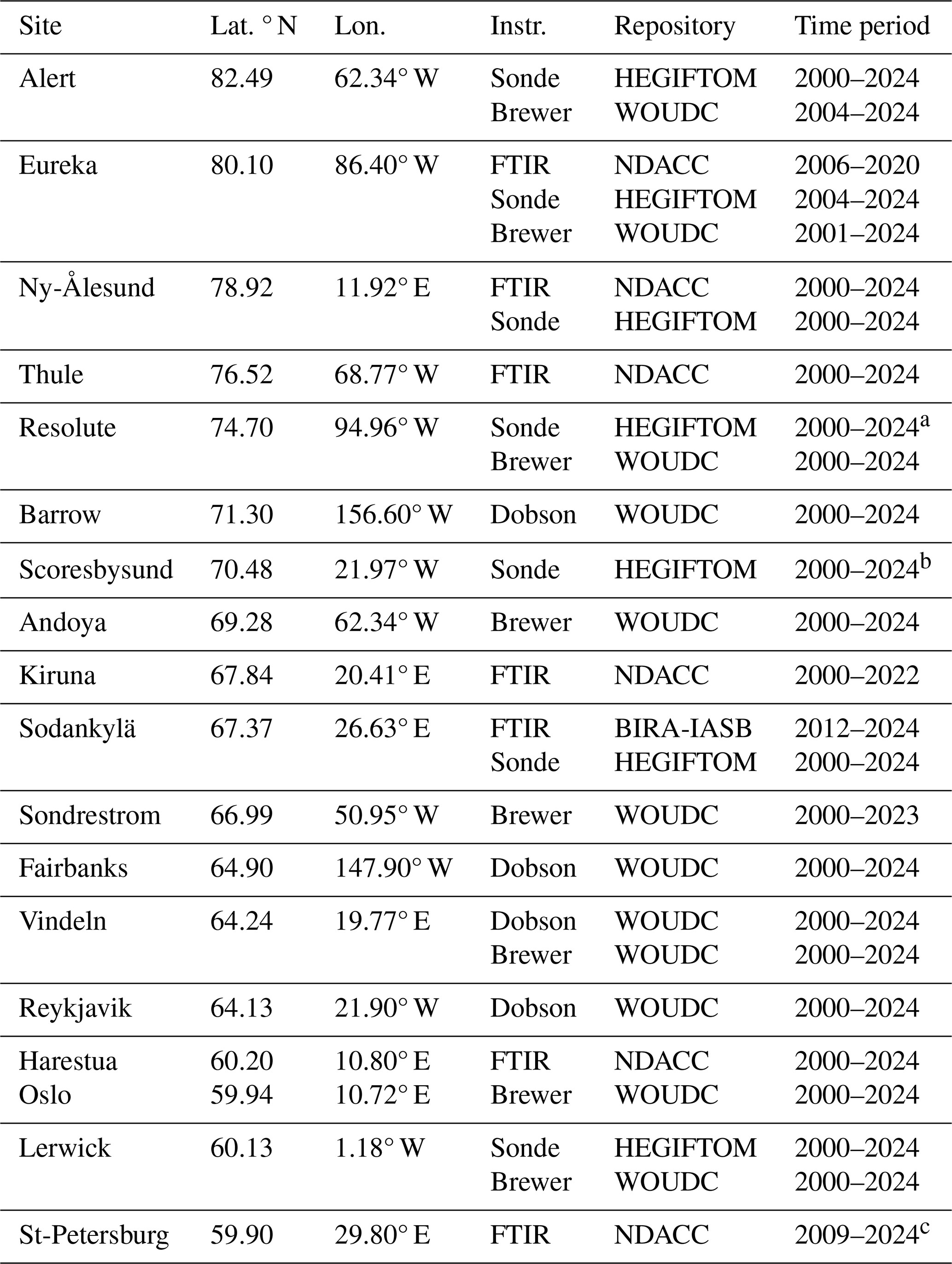
a Resolute's is restricted to the 2005–2024 time period for reason detailed in the comparison with satellites, see Sect. 3. b Scoresbysund's time series is not used at all in the trend analysis for reasons also detailed in Sect. 3. c In the lower stratosphere, St-Petersburg's is not used in the trend analysis because it cannot be merged with other data sets there and it only starts in 2009.
For all time series, the uncertainty on ozone partial columns is obtained from the propagation of the retrieved profile uncertainties. Random and systematic uncertainties are themselves obtained using optimal estimation (Rodgers, 2000; Vigouroux et al., 2015). The random error of partial columns additionally contains a smoothing error (Rodgers, 2000) estimated from the WACCMv7 covariance matrix at each site. In Table 1 we provide the mean of the obtained uncertainties in percent for each partial column considered in this paper and the total column of ozone (TCO). The partial columns are based on FTIR DOFS that are explicitly given here for NDACC products and for the Sodankylä product.
2.2 Ozonesondes
Ozonesondes are small, light-weight devices flown on weather balloons that measure the vertical profile of ozone based on the titration of ozone in a neutral buffered potassium iodide sensing solution, with a precision better than ± (3–5) % and an accuracy of approximately ± (5–10) % for up to 30 km altitude (Smit et al., 2024). However, changes in preparation and operation procedures, manufacturer type, sensing solution strength, and processing might result in biases in the time series, compromising any reliable ozone trends assessment. Therefore, a homogenization activity, correcting for those biases following recommendations in Smit et al. (2021) and Smit and the O3S-DQA Panel (2012) has been undertaken, with all the homogenized ozonesonde data stored and described within the framework of the Tropospheric Ozone Assessment Report Phase II (TOAR-II) Focus Working Group HEGIFTOM (Harmonization and Evaluation of Ground-based Instruments for Free-Tropospheric Ozone Measurements, see also Van Malderen et al., 2025a). In that study, the data from the Canadian Arctic sites Resolute, Alert, and Eureka and the European Arctic sites Scoresbysund, Ny-Ålesund, Sodankylä and Lerwick have been used. More details on the specific homogenization steps needed to correct those data sets are provided in Tarasick et al. (2016) for Resolute, Alert, and Eureka and in Nilsen et al. (2024) for Scoresbysund, Ny-Ålesund, and Sodankylä.
In this study, we cap sondes profiles at 26 km so that the mid-stratospheric column contains at least 60 % of all measured profiles at all sites (in some sites such as Alert and Resolute, less than 50 % to 40 % of profiles reach up to 30 km because the sondes balloon burst before that altitude). We sum profiles over the partial columns defined in Sect. 2.4. Random measurement uncertainties on profile points are also propagated to obtain partial columns uncertainties. When a profile doesn't provide uncertainties, we use the mean uncertainties of other profiles from the same site. Extreme outliers are found in the data after summing the profiles into partial columns. They are removed by applying a very loose percentile filter: for q1 and q3 the 25th and 75th percentiles, we remove datapoints lying beyond or below for each partial column time series.
2.3 Brewer and Dobson spectrophotometers
Brewer and Dobson spectrophotometers use sunlight in the UV range (approximately 305–340 nm) to extract the total column of ozone by comparing relative intensities for pairs of selected wavelengths. All Brewer and Dobson total column data sets used in this study are obtained from the World Ozone and Ultraviolet Radiation Data Centre (WOUDC), one of six World Data Centres part of the Global Atmosphere Watch programme of the World Meteorological Organization. It provides total column ozone and vertical profile data from over 500 registered stations (https://woudc.org/, last access: 8 June 2026). We use Brewer total column measurements from Resolute, Sondrestrom, Alert, Eureka, Vindeln, Oslo, Andoya and Dobson total column measurements from Lerwick, Barrow, Reykjavik, Fairbanks and Vindeln. They are given as daily measurements obtained from several measurements averaged together with a standard deviation estimate. When the standard deviation is not provided, we use a generic random error of 1 % for direct sun observation (DS) and 5 % for other types of measurement (zenith-sun ZS, focused-moon FM) (see e.g., Fioletov et al., 2005; Vogler et al., 2007). The Brewer in Alert has calibration issues concerning ZS measurements so these are excluded from the dataset. For all Brewer measurements we restrict to airmass factors μ<3.5 for single monochromator instruments (MKII, MKIV and MKV). Finally, most stations have measurements taken by several instruments, so we average all same-day observations with a weighted mean.
2.4 Choice of partial columns
While Dobson and Brewer data sets only provide a total column measurement of the ozone abundance, ozonesondes and FTIR present vertically-resolved profiles. Since this vertical resolution only contains four to five DOFS for the FTIR, we divide the troposphere and stratosphere into four layers (see Table 3) to obtain four partial columns of ozone, each containing approximately one DOFS for the FTIR (see Table 1). The specific choice of boundaries for these layers reflects the need for merging FTIR with sonde data sets.
Table 3Altitude layers defining the four partial columns of ozone considered for ozonesondes and FTIR. Partial columns are calculated from profiles using the altitude in kilometers. The CAMS grid line reports the approximate equivalent pressure layers used for calculating partial columns of CAMS data in the representativeness study (see Sect. 4). The last line summarizes which data sets are used in each partial column of this study. The asterisk next to FTIR means that the lower-resolution product at Sodankylä is excluded.
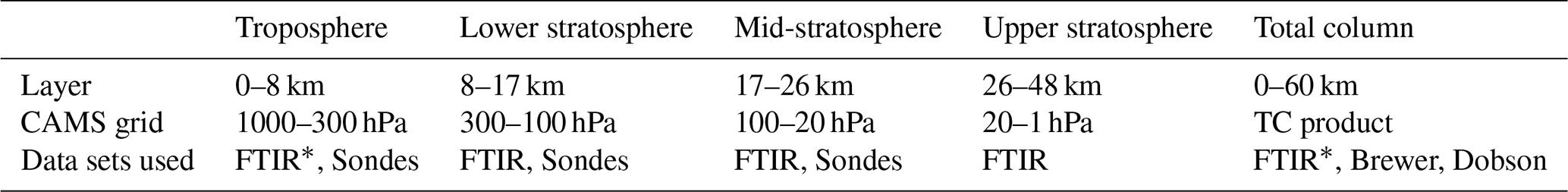
Since we work with fixed altitudes defining partial columns boundaries, we do not follow the tropopause variations in time. Note that since FTIR provides low-resolution profiles, a clear-cut disentanglement of tropospheric and lower-stratospheric measurements is impossible and some mixing is necessarily present. The choice of 0–8 km reflects the averaged Arctic tropopause limit (Zängl and Hoinka, 2001) while satisfying the constraint on FTIR DOFS.
In addition to the partial columns defined in Table 3, we consider an alternative lower stratospheric column from 10–17 km in Sect. 3 to ease comparison to satellite products, plus another upper stratospheric column from 32–48 km in Sect. 5 to better compare with trend literature that often considers the upper stratospheric layer higher up.
From those ozone columns we first calculate daily mean time series, and from those we obtain monthly mean time series. We then use the monthly mean time series to calculate relative (Eq. 1) and absolute (Eq. 2) anomalies:
with
the ozone mean for each month of the year averaging over n years of each data set, from start year to start year+n. Using anomalies when merging different data sets instead of monthly means removes the issues related to merging biased data
3.1 Satellite data sets and method
We use comparisons with two different satellite data sets, IASI-CDR and MEGRIDOP, to investigate the quality of all the ground-based time series described above and to evaluate the presence of drifts in satellites for the whole Arctic zonal mean (i.e., a weighted mean of all ground-based stations datasets within the 60–90° N region), both in the total column and for each partial column defined in Sect. 2.4.
The IASI-CDR dataset is a homogeneous ozone Climate Data Record (CDR) based on the Infrared Atmospheric Sounding Interferometer observations recently produced by EUMETSAT on behalf of AC SAF (AC SAF, 2025). The IASI-CDR O3 product has been validated in Boynard et al. (2025), who reported small total ozone biases (< 1 %–2 %), tropospheric differences of 10 %–12 %, and long-term drifts below 3 % per decade. It accurately captures seasonal and interannual variability and highlights a decrease in tropospheric ozone, notably in the tropics and Europe. Here, IASI-CDR O3 total columns are obtained from the combined AERIS Level-3 monthly IASI-CDR Metop-A (2007–2013) and Metop-B (2013–2024) products, called hereafter IASI-A + B (Clerbaux and Coheur, 2025a, b). Partial columns are derived from merged monthly mean gridded profiles computed from the AERIS Level-2 daily IASI-CDR Metop-A and B products as in Keppens et al. (2025), called IASI-AB hereafter. Both data sets cover 2007–2024 and we use daytime observations only.
The MErged GRIdded Dataset of Ozone Profiles (MEGRIDOP) (Sofieva et al., 2021) was generated using data from six limb and occultation satellite instruments (OSIRIS, GOMOS, MIPAS, SCIAMACHY, Aura MLS, OMPS-LP SNPP). We use the Level-3 gridded monthly time series from 2001 until 2024, which has a 10° lat. × 20° lon. horizontal resolution and a vertical coverage from 10–50 km.
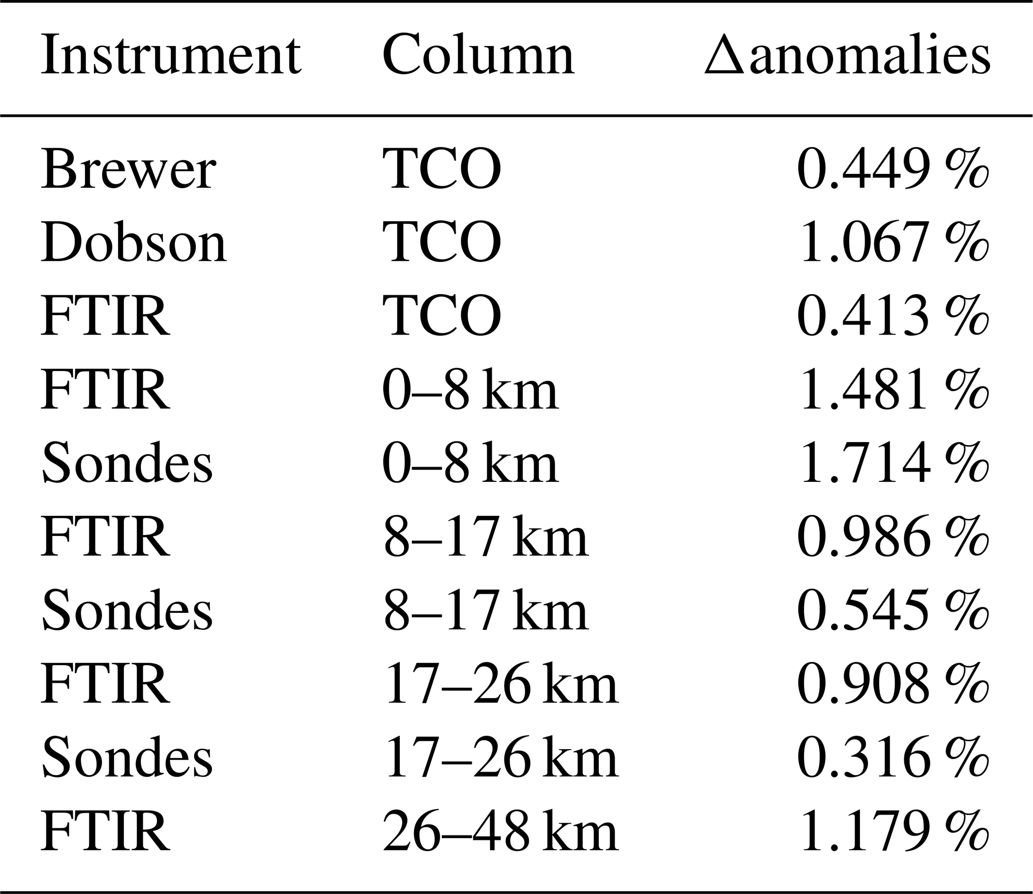
Our aim here is not to validate the satellite products but rather to compare satellite and ground-based time series to diagnose potential problems related to the calculation of trends from those time series. Therefore, we do not time-collocate satellites and ground-based measurements but instead we compute drifts by comparing monthly deseasonalized relative anomalies, that will later be used for trends computations. The time series of satellites are spatially collocated within their respective spatial grid with the ground-based instruments locations listed in Table 2. To compare satellite and ground-based time series, we define the difference of anomalies in percent:
from which we obtain the relative bias and the scaled mean absolute deviation (MADs) between the two time series (scaling with 1.4826 gives an equivalence to the 2σ of Gaussian statistics):
We then apply a robust linear regression (Theil-Sen method, Sen, 1968) on the difference (Eq. 4) to obtain the trend of this difference, i.e., the drift and its associated error, as shown in Fig. 2 for the Vindeln Brewer against IASI-A + B ozone total column.
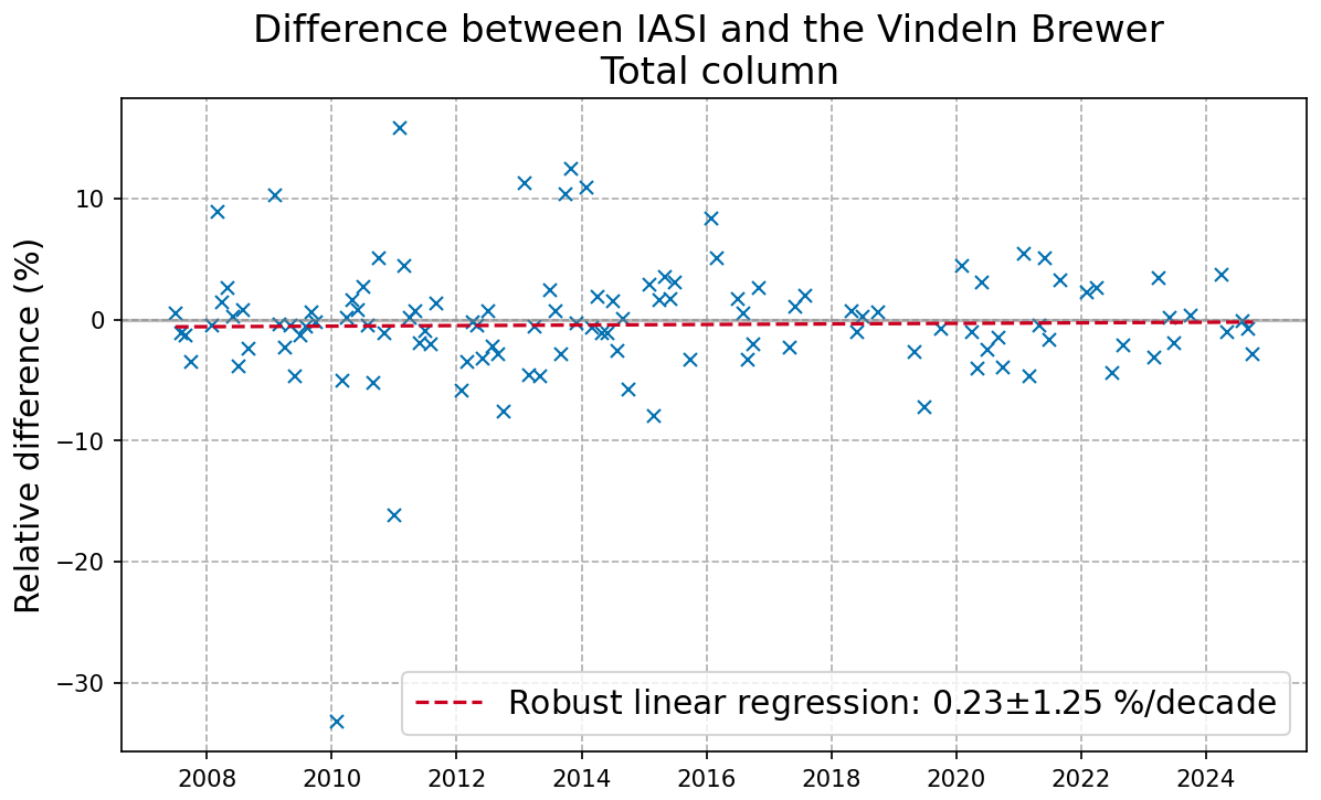
Figure 2Difference of relative anomalies in percent (Eq. 4) between the Vindeln Brewer total column and the IASI-A + B total column in Vindeln. The trend of this difference is represented by the red dashed line and corresponds to the drift, given in legend with its 2σ-error. The presence of several strong outliers requires the use of a robust regression method, here the Theil-Sen method.
The drift is estimated as the median of the slopes of all lines connecting all possible pairs of points. The standard Theil-Sen confidence interval estimates assume the time series have no autocorrelation, but by computing the autocorrelation on the regression residuals (as the Pearson correlation coefficient between the residuals at t and at ), we find that 13 % of our data sets have an autocorrelation comprised between 0.2 and 0.35 in absolute value. To rigorously account for this small autocorrelation, we have therefore applied the block bootstrap method (Gilda, 2024) to evaluate the confidence intervals of our estimated Theil-Sen drifts (Bontempi, 2024). We have used 1000 bootstrap samples and a block size of , where n is the length of the dataset. The Theil-Sen method was applied on each bootstrap sample. The 2σ-error estimate given for each drift value corresponds to the 95 % confidence interval, calculated by multiplying the square root of the bootstrap estimate of variance by z=1.96, i.e. the inverse of the standard normal cumulative distribution function , where α=0.95.
We make the assumption that problems in individual stations data sets can be identified by comparing to the two satellite data sets, while drifts in individual satellite dataset can be identified with combined ground-based data sets. In Sect. 3.2, we validate each individual ground-based dataset by detecting outliers in the drifts with respect to satellites, and then in Sect. 3.3, we evaluate satellites by computing their Arctic zonal mean drift with respect to the weighted mean of all validated ground-based time series.
3.2 Evaluation of ground-based time series from satellite comparison
MEGRIDOP is based on Limb satellites that do not measure in the troposphere, so ground-based measurements of the tropospheric column and the total column can only be compared to IASI-CDR (see Fig. 3 for a visual representation of the vertical coverage of profile data sets versus the chosen partial column layers). Moreover, because MEGRIDOP only starts at 10 km, we consider an alternative lower stratospheric column from 10–17 km. This alternative lower stratospheric partial column can be easily computed and still retains enough DOFS for the FTIR (see Table 1). The reason why we selected 8–17 km as our main lower stratosphere column is because we want to be able to compare total column trends to the sum of partial column trends.
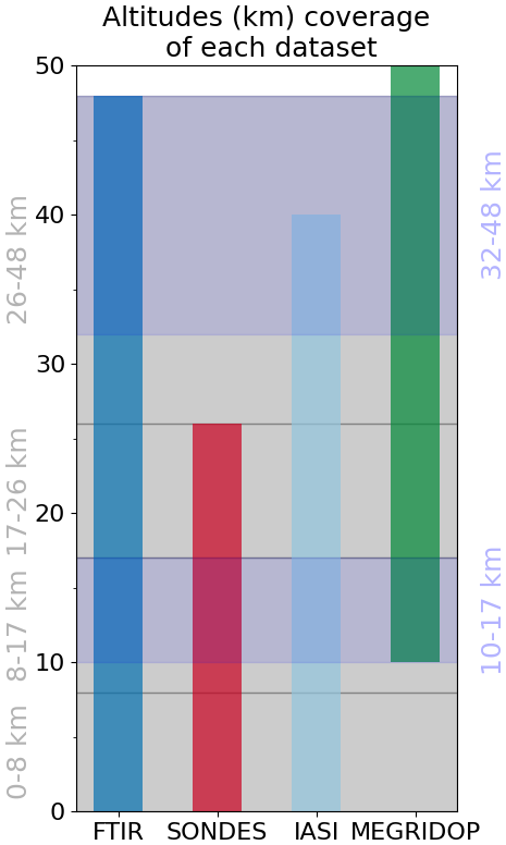
Figure 3Vertical coverage in kilometers of each profile data sets used in this study against our choice for partial columns altitude boundaries in grey on the left. Additional alternative partial columns are shown in blue on the right. The choice of partial columns boundaries is explained in Sect. 2.4.
We do not identify any outliers in the total column ground-based time series. We find all drifts lay within (see Fig. 4). Only the drifts in Fairbanks and Kiruna are at the limit of 2σ significance, reaching respectively % per decade and % per decade. Although it might indicate potential issues in those timeseries around 2007, we do not exclude them from our trend analysis, as these drift values are small and we will in fact consider the full 2000–2024 period for trends.
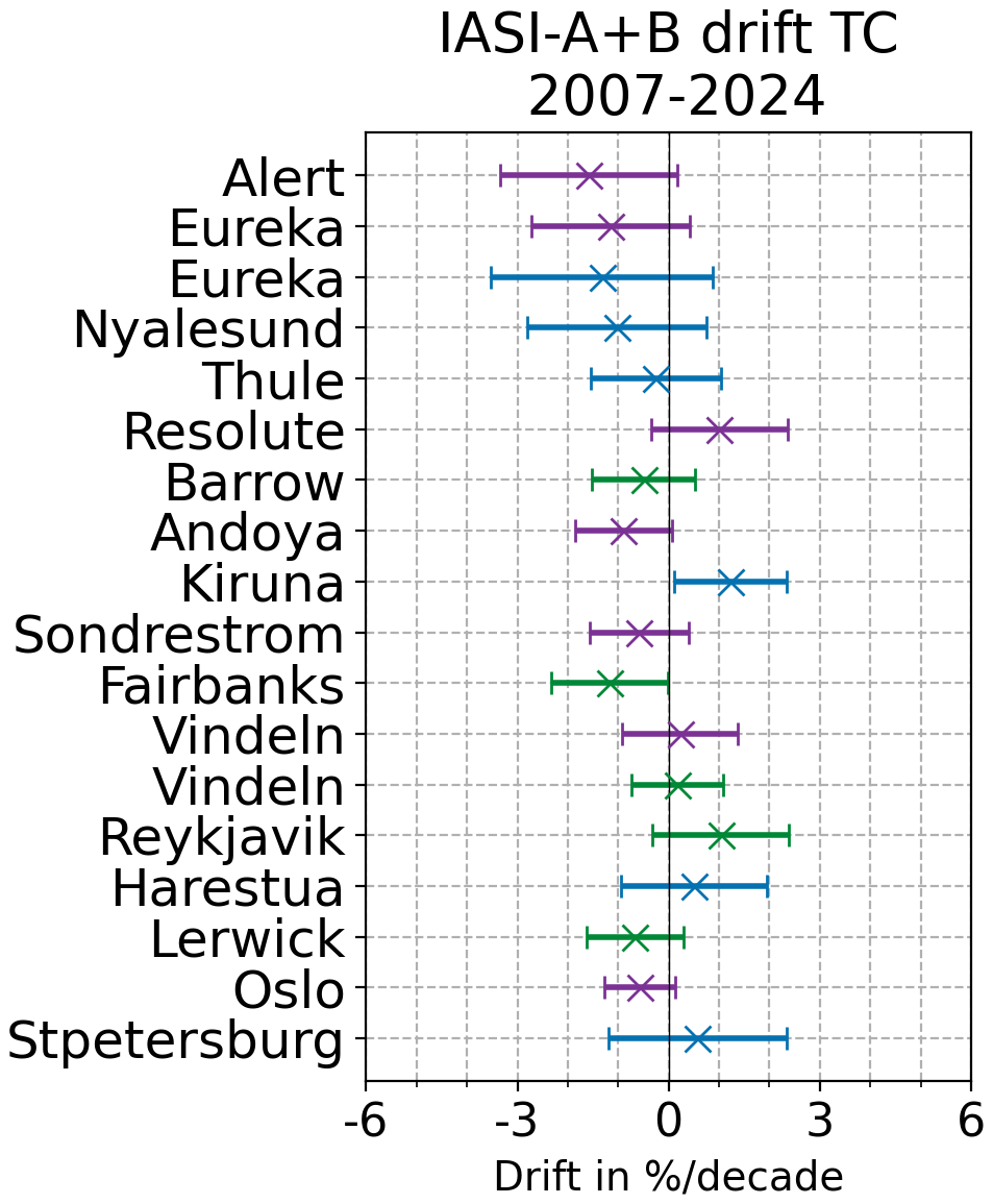
Figure 4Robust drift of IASI-CDR on the full 2007–2024 period for the total column with respect to all individual FTIR, Brewer and Dobson instruments in percent per decade, with a 2σ-error. Instruments are ordered by decreasing latitude from top to bottom, and trends are color-coded depending on the instrument (purple: Brewer, green: Dobson, blue: FTIR).
In the troposphere, IASI-CDR exhibits a significant negative drift of at least −5 % per decade with seven of the ground-based instruments (see Fig. 5). The Scoresbysund sonde stands out as the only significant positive drift of IASI, signaling an issue with this ground-based dataset. We checked that this large drift is not due to a different of time-sampling between the sonde data sets and the satellites: applying different filters on the minimal number of sonde measurements per month doesn't change the drifts values.
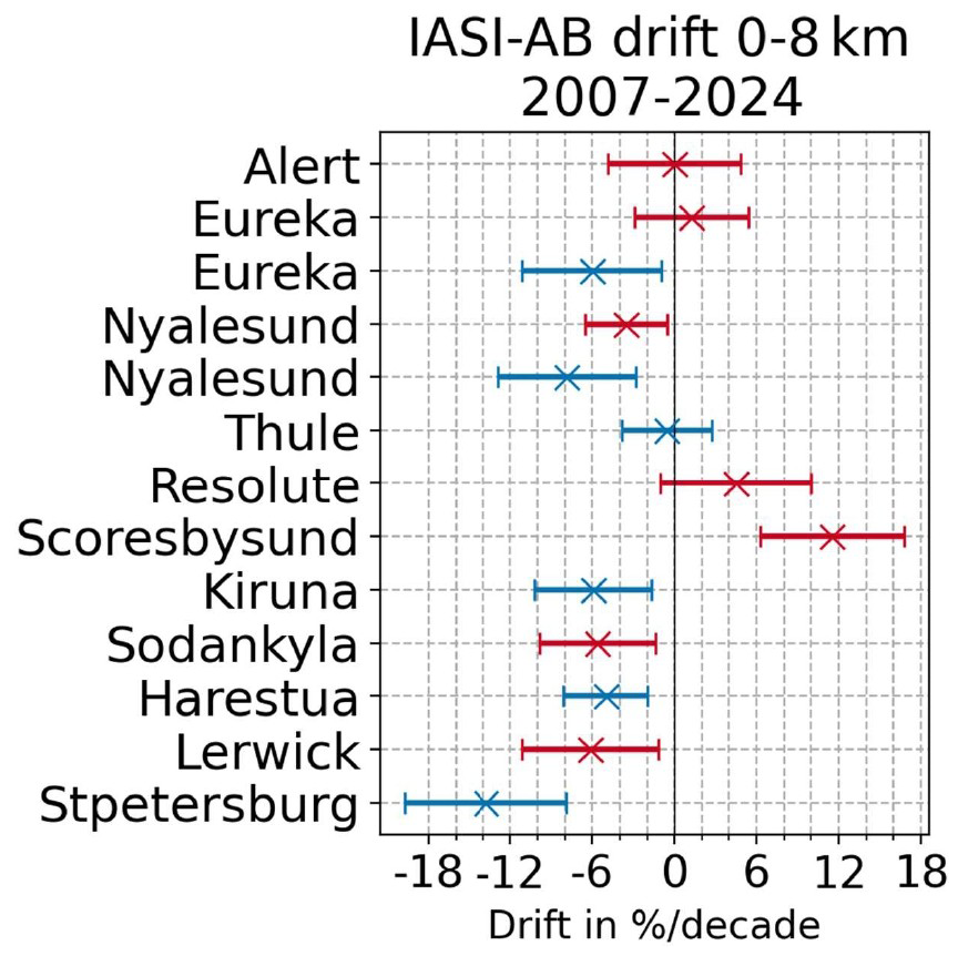
Figure 5Robust drift of IASI for the troposphere with respect to all individual FTIR and Sonde instruments in percent per decade with 2σ-error. As in Fig. 4, instruments are ordered by decreasing latitude from top to bottom, and trends are color-coded depending on the instrument (blue: FTIR, red: Sondes).
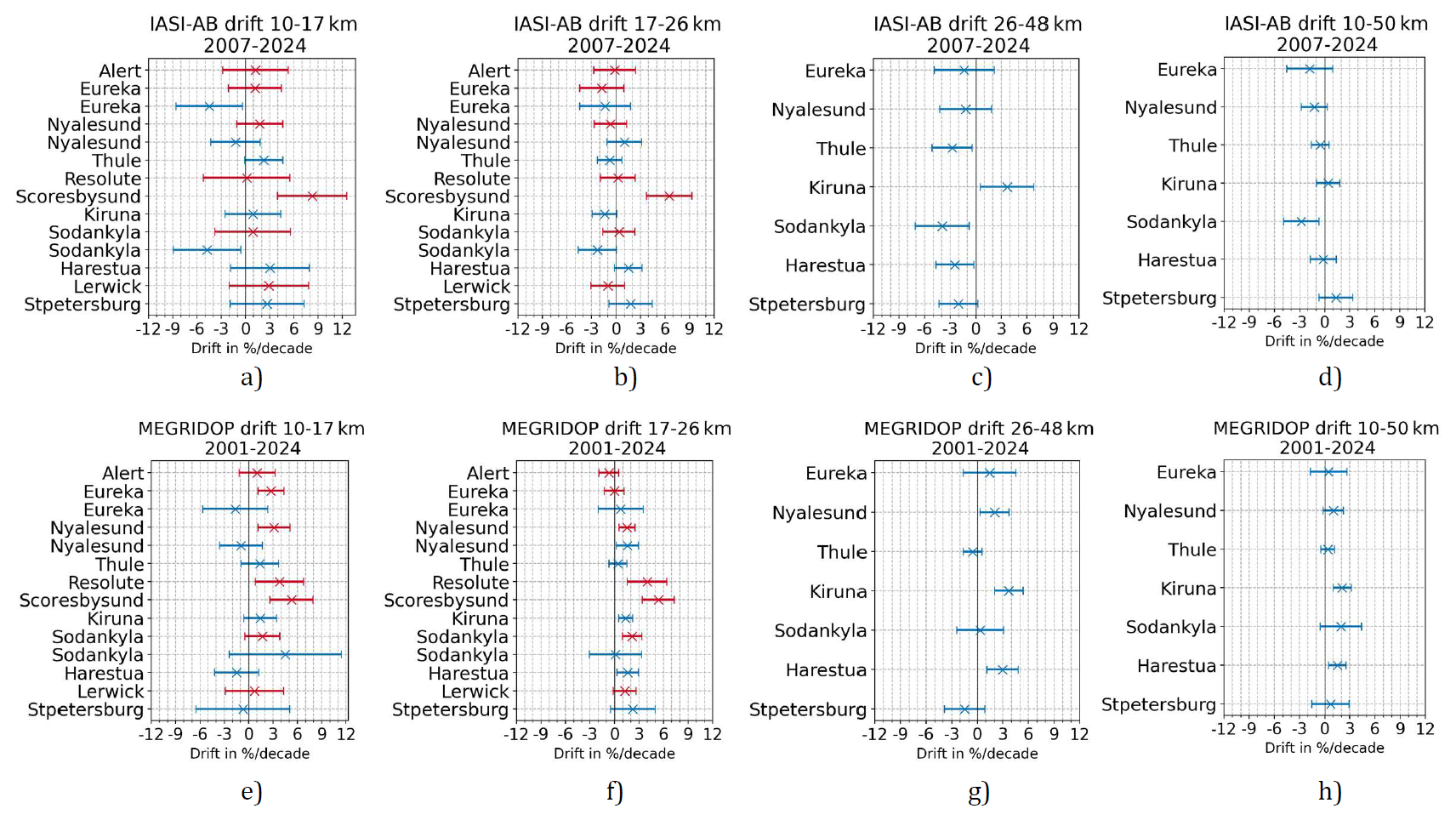
Figure 6Robust drifts of IASI-CDR (a–d) and MEGRIDOP (e–h), with respect to ground-based measurements for stratospheric partial columns. Drifts are in percent per decade with 2σ-error. Note that the time periods given in the title of each figure refers to the satellite time periods, but some ground-based time series are more limited, see Table 2.
Turning to the stratospheric column drifts of both IASI (on the 2007–2024 period) and MEGRIDOP (on the 2001–2024 period) with respect to all individual ground-based instruments in Fig. 6, we find that the Scoresbysund sonde also stands as an outlier in the lower and mid-stratosphere for both satellites. The drift is associated with a negative offset in the Scoresbysund ozone concentrations at most altitude levels in the ozonesonde time series since 2016 with respect to the previous years. Indeed, we have verified that the Scoresbysund's sonde dataset does not show any significant drift with respect to MEGRIDOP over the prior 2001–2015 period, where we found a drift of approximately 4 % per decade in the 10–17 km layer and of approximately 2 % per decade in the 17–26 km layer, both non-significant. This drop in 2016 coincides with a change of ozonesonde pump battery and pump temperature sensor types, possibly responsible for the lower recorded pump temperatures (around −10 K), and a radiosonde type change, creating a possible offset in the atmospheric pressure measurements (switch from pressure sensor to GPS height-derived pressure measurements). Too low pump temperatures might point to freezing solutions and too low signal readings, as noted at another ozonesonde site (Okamoto et al., 2026), and the radiosonde pressure offset might shift of the entire profile with +1.5 hPa at mid-stratospheric pressure levels. A total column ozone drop-off of −5.6 % with respect to OMI satellite overpass measurements has been mentioned for Scoresbysund around 2016 (change of ozonesonde serial batch number) in Stauffer et al. (2022), but the operational, non-homogenized, time series was used in that study. Therefore, at least a part of this drop-off is due to the fact that a −3 % to −4 % ozone bias correction has been implemented in the vertical profiles (transfer functions defined in Deshler et al., 2017) of the non-homogenized time series from 2016 onwards only, although it should also have been applied to earlier parts of the time series (e.g. from mid 2001 to 2015), as it has been done in the homogenized time series used here. Unfortunately, the homogenization did not seem to resolve all issues occurring around 2016, which need further investigation and the development of adequate correction algorithms, so we remove the Scoresbysund ozonesonde dataset from our study.
The Resolute sonde also appears as an outlier in MEGRIDOP's drifts for the lower and mid-stratosphere but not in IASI-CDR's drifts. By comparing the drifts on the same time period (2007–2024), the MEGRIDOP's drifts at Resolute disappear, see Fig. 7. In fact, we see a progressive diminution of the drift that becomes non-significant starting from 2005. This is probably the signal of a jump in the sonde dataset possibly due to instrumentation changes. Recalibrations in the data sets to account for these various changes have already been performed in Resolute (see Tarasick et al., 2016) but additional jumps cannot be excluded. Despite these recalibrations, it was found in Fig. 17 of Tarasick et al. (2016) and Fig. 3 of Nilsen et al. (2024) that the Resolute sonde exhibits stronger significant negative trends in the lower stratosphere than other sondes in the Arctic (except for the Churchill sonde that lies equatorward). To avoid effects of this potential jump, we consider the Resolute sonde dataset only starting from 2005.
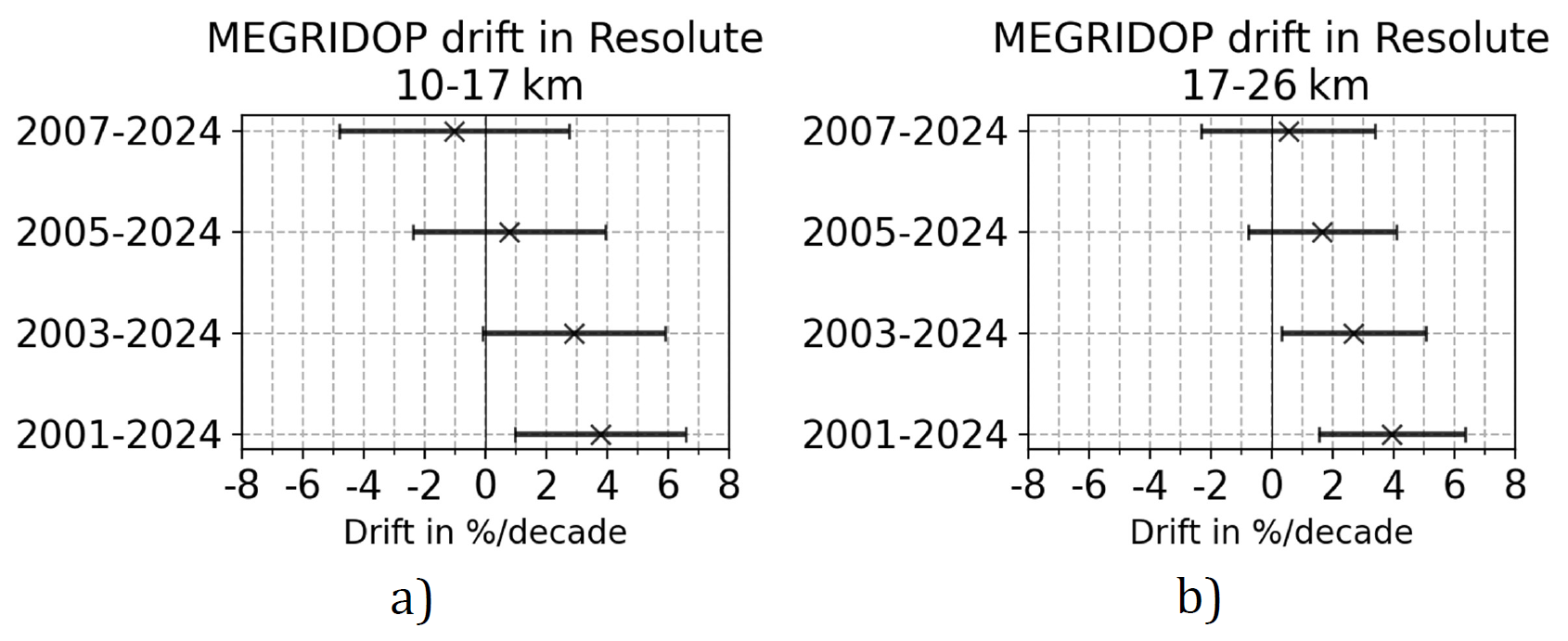
Figure 7Variation of the drift of MEGRIDOP with respect to the Resolute sonde in the lower (a) and mid (b) stratospheric columns, depending on the starting date of comparison.
In the upper stratosphere (26–48 km, Fig. 6), IASI-CDR possesses small negative drifts everywhere except at Kiruna, where it shows a singular significant positive drift above 3 % per decade. The drift of MEGRIDOP in Kiruna doesn't particularly stand out on the 2001–2024 period, but if we restrict both satellites to the same 2007–2022 time period (Kiruna time series stops in 2022, see Table 2), we observe a similar pattern where all drifts are non-significant and within 3 % per decade except in Kiruna where they reach 3.65±2.97 % per decade for IASI-CDR and 4.92±2.58 % per decade for MEGRIDOP, see Fig. 8. There are no records of possible issues with the Kiruna FTIR time series and visual scrutiny of its monthly mean and anomalies time series doesn't reveal obvious jumps. As the drift value with MEGRIDOP using the full time series (Fig. 6) is comparable to other FTIR stations (although significant at Kiruna), we retain Kiruna for our trend analysis on the full time period.
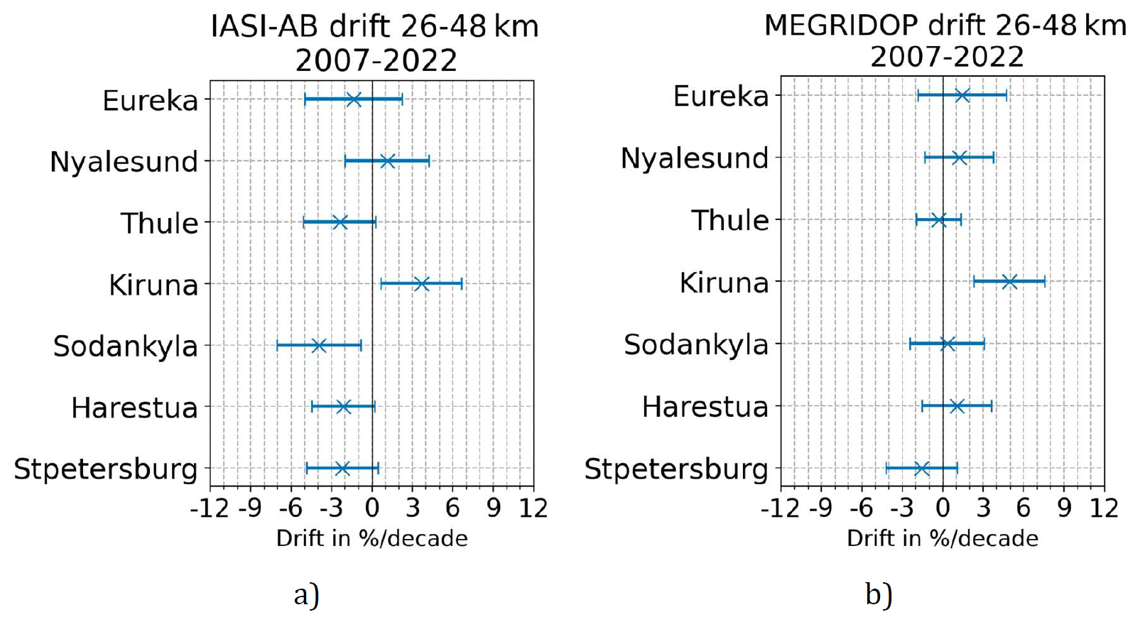
Figure 8Drifts of IASI-CDR (a) and MEGRIDOP (b) with respect to the FTIR data sets in the upper stratosphere when restricting to a common period of 2007 to 2022.
Finally, in the total stratospheric column (10–50 km, Fig. 6), IASI-CDR does not exhibit any significant drift except with the FTIR at Sodankylä. That time series is retrieved from a different spectral range than other NDACC FTIR products but there is no trace in previous studies of a potential drift due to this method of retrieval (García et al., 2014; Zhou et al., 2020). It is also the only time series that starts in 2012 so the starting date for IASI-CDR comparison is different from all other data sets.
3.3 Drift of satellites for the Arctic zonal mean
Having set aside ground-based time series with identified problems, we average all remaining data sets by a weighted mean (weights are given by the inverse squared uncertainties), and compare this average with the mean of satellites time series at the site locations. The resulting zonal mean drifts of IASI-CDR and MEGRIDOP are presented in Fig. 9.
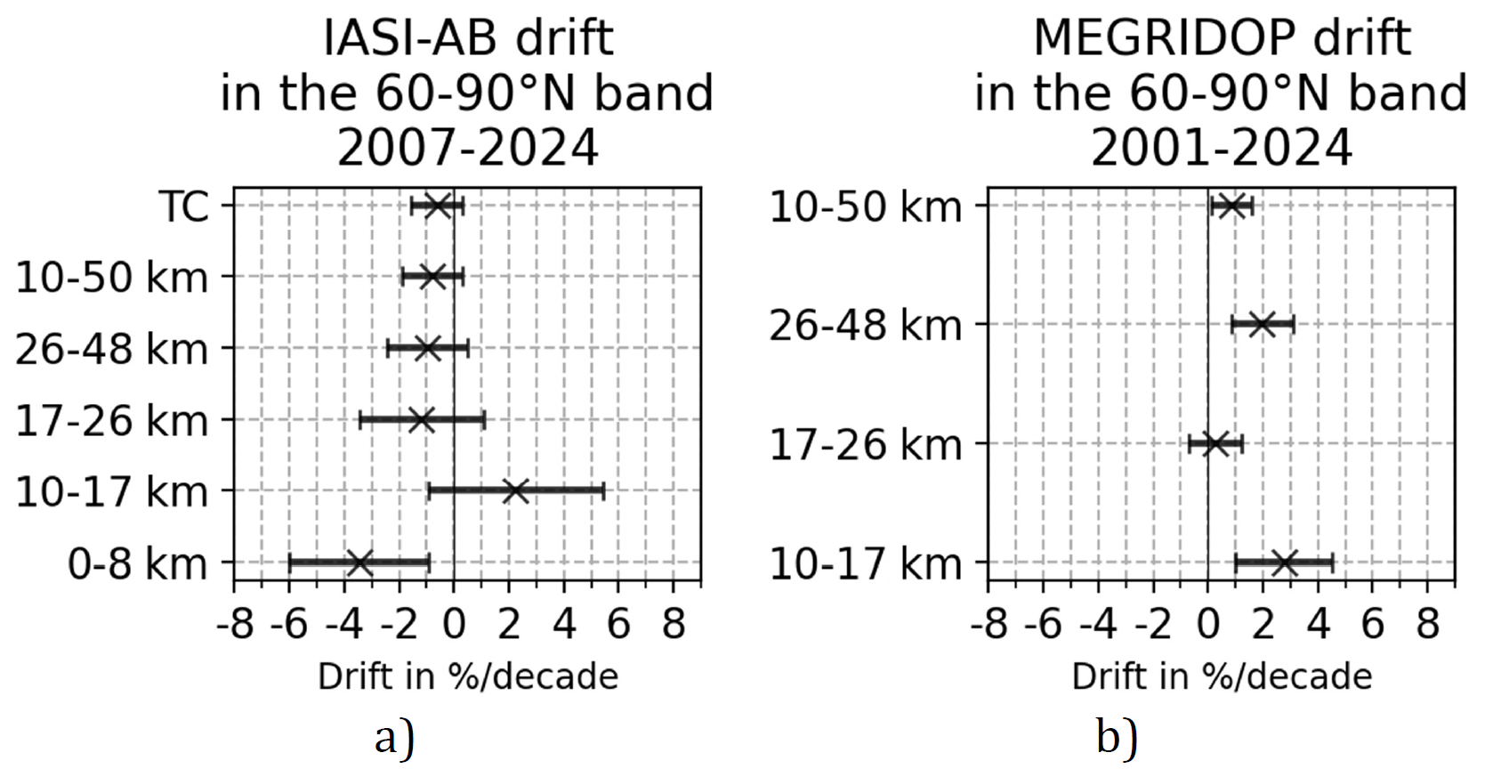
Figure 9Drifts of satellites with respect to the zonal (weighted) means of all ground-based instruments in each column. Ground-based instruments with identified problems (Scoresbysund sonde, Resolute sonde before 2005) are not included in the means.
The zonal mean drift of IASI-CDR total column is of % per decade. This is a very small uncertainty and it shows that the IASI-CDR Level 3 AERIS total column product doesn't show a drift over its full time series.
In the troposphere we find a negative significant drift of IASI-CDR of % per decade. Since the sensitivity of IASI in the troposphere is low, with an average number of DOFs <0.45, the a priori has a strong influence on the retrieved measurements in the troposphere. Degrading the ground-based data sets to the IASI sensitivity by smoothing their profiles with the IASI averaging kernels (Rodgers and Connor, 2003) was found to shift the IASI drift by −2.3 % per decade on average in the Arctic troposphere in Boynard et al. (2025). However, the smoothing formula must be performed on each individual profiles: the averaging kernel are non-linear objects and smoothing averaged monthly data is not equivalent to averaging individually smoothed profiles, and can introduce additional errors. We therefore do not smooth the ground-based data sets here. This means that we probably underestimate the tropospheric IASI drift by 2 %. Note that the much smaller drift obtained by Boynard et al. (2025) in the Arctic troposphere of −1.5±1.8 % per decade is biased due to the use of the Scoresbysund sonde dataset in the validation, see the Table S1 of Boynard et al. (2025) with individual stations drifts. By excluding this dataset and including FTIR, we find a larger and significant drift of the IASI Arctic troposphere. A more detailed validation using time-collocated pairs of smoothed Level-2 measurements is necessary to evaluate the exact amplitude of this drift and whether it represents a real stability issue.
IASI-CDR doesn't show any significant drift in the lower, middle and total stratosphere. In the lower stratosphere the individual drifts are all within , with a zonal mean drift of 2.25±3.17 % per decade. In the middle and total stratosphere individual drifts lay within , with a zonal mean drift of % per decade and % per decade, respectively.
The MEGRIDOP data shows a positive drift with respect to the zonal mean of all ground-based instruments in the lower and upper stratosphere with drifts of 2.76±1.77 % per decade and 1.97±1.18 % per decade, respectively. The smallness of the uncertainties reinforces our assumption that the zonal mean drift captures the true satellite drifts, while averaging out individual ground-based instruments errors and drifts.
In the mid-stratosphere, the zonal mean drift of MEGRIDOP is only 0.27±0.96 % per decade while all individual drifts lay within .
Finally, in the total stratospheric column, MEGRIDOP's zonal mean drift is slightly positive significant: 0.88±0.73 % per decade. All individual drifts are within . The smallness of the uncertainty is here also remarkable, but is expected to be smaller in MEGRIDOP than for IASI-CDR since the time period of comparison is more extended.
3.4 Conclusions on ground-based versus satellite comparisons
-
The Scoresbysund sonde is strongly negatively drifted. The drift is probably associated with the many instrumental changes around 2016 that cannot be fully corrected for. This is important as this sonde was used in the past for validation of satellites whose drift could have been overestimated or underestimated accordingly, as in Boynard et al. (2025). We don't use this time series in our trend analysis.
-
We find hints of a potential jump in the Resolute sonde dataset before 2005, possibly due to instrumentation changes. We restrict this time series to 2005–2024 for the trend analysis.
-
In the Arctic zonal mean, both satellites drifts are smaller than for all stratospheric columns.
-
IASI-CDR possesses a significant drift only in the troposphere, where its zonal mean drift reaches % per decade without smoothing. The effect of smoothing cannot be applied on monthly averaged measurements trustfully, but has been shown to shift the drift by −2.3 % per decade on average in the Arctic troposphere (Boynard et al., 2025). A careful validation on time-collocated smoothed Level-2 measurements is necessary to determine if this drift indeed exceeds the stability threshold of tropospheric ozone (Weber, 2024).
-
MEGRIDOP shows significant positive drifts for the zonal mean in the lower, upper and total stratosphere of 2.76±1.77 % per decade, 1.97±1.18 % per decade and 0.88±0.73 % per decade, respectively. These values, and in particular their very small associated uncertainties, constitute important results concerning the stability of the MEGRIDOP product, which is used in the Long-term Ozone Trends and Uncertainties in the Stratosphere (LOTUS) initiative.
An important drawback of ground-based measurements of atmospheric species compared to satellites measurements is the coarse spatial coverage of the data. Despite the use of various instrument types, in this study we only consider sixteen different sites where ozone is measured over a sufficiently long time period, spanning a region from 60 to 90° N, equivalent to a surface area of 34×106 km2. On the other hand, the long-term trends we are trying to observe are known to be small and hiding behind the large natural variability of ozone in the Arctic. To reduce uncertainties and obtain statistically significant trends, it is advantageous to combine several data sets which are geographically close. But what is a good criterion to combine data sets together? And what will be the spatial extent that the trends obtained from these combined data sets can actually represent? To answer these questions, we perform a representativeness study following Weatherhead et al. (2017). A similar representativeness study based on CAMS data for ozone but limited to the troposphere was also conducted in Van Malderen et al. (2025b). We use the CAMS global reanalysis (EAC4) monthly averaged fields (Inness et al., 2019) of ozone to calculate the correlation of ozone time series between the locations of each of our ground-based stations. This assumes that correlations are not only due to inter-annual variability, but that since we are comparing the same variables (i.e., ozone anomalies) at different locations, the same physical processes are causing the variability, so that similar trends are expected for largely correlated locations. This enables us to define groups of stations that are highly correlated, and for which we create merged ground-based data sets whose trends are studied in Sect. 5. We further refine the regional representativeness of those groups of stations by calculating the correlations of CAMS ozone time series at those stations with CAMS ozone time series in the rest of the Arctic. The CAMS dataset is a gridded dataset with a global coverage, a spatial resolution of 0.75° × 0.75° and a temporal coverage from 2003–2024. We use the ozone total column and the vertically gridded ozone profile given in 25 pressure levels that we sum in four partial columns as shown in Table 3.
Correlations are calculated based on monthly deseasonalized absolute anomaly (Eq. 2) time series because correlations of ozone column time series would mostly reflect the seasonal cycle of ozone. Therefore, the correlations represent the similarity in ozone variability independent of the seasonal cycle. For each ground-based station, we compute the Pearson correlation coefficient rx,y between the CAMS monthly anomaly at the grid-cell where that site is located, x, and the CAMS monthly anomalies for each of all the other cells, y, located in the Arctic between 60–90° N. We have verified the consistency of our results by analyzing the scatterplots of absolute anomalies between each ground-based station location.
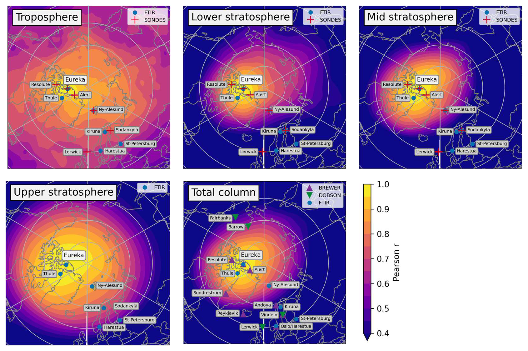
Figure 10Correlation of CAMS deseasonalized anomalies at the location of the Eureka station with CAMS anomalies in the rest of the Arctic for the 4 partial columns and the total column of Table 3. Stations where a ground-based instrument is used in the corresponding partial column are indicated.
We obtain correlation maps (see Fig. 10) at each ground-based station for the total column and the four partial columns of ozone. We consider each of these columns separately in this analysis because they all entail different sets of ground-based instruments (see Table 3) but also because the atmospheric dynamics and ozone chemistry vary with altitude, impacting the size of correlated regions in each layer. In the lower and mid-stratosphere (8–26 km), we find that regions with correlated ozone anomalies are smaller in extent than in the upper stratosphere, above 26 km. This is expected since photochemistry drives ozone variability in the upper stratosphere, while in the lower and mid-stratosphere, dynamical activity dominates variability (Brasseur and Solomon, 2005). In the troposphere, very highly correlated regions (r>0.95) are small like in the lower stratosphere, but correlated regions with are very spread out. This is consistent with the fact that photochemical processes dominate ozone variability in the troposphere (Cooper et al., 2014) and that emissions of ozone precursors are low and relatively homogeneous across the 70–90° N region.
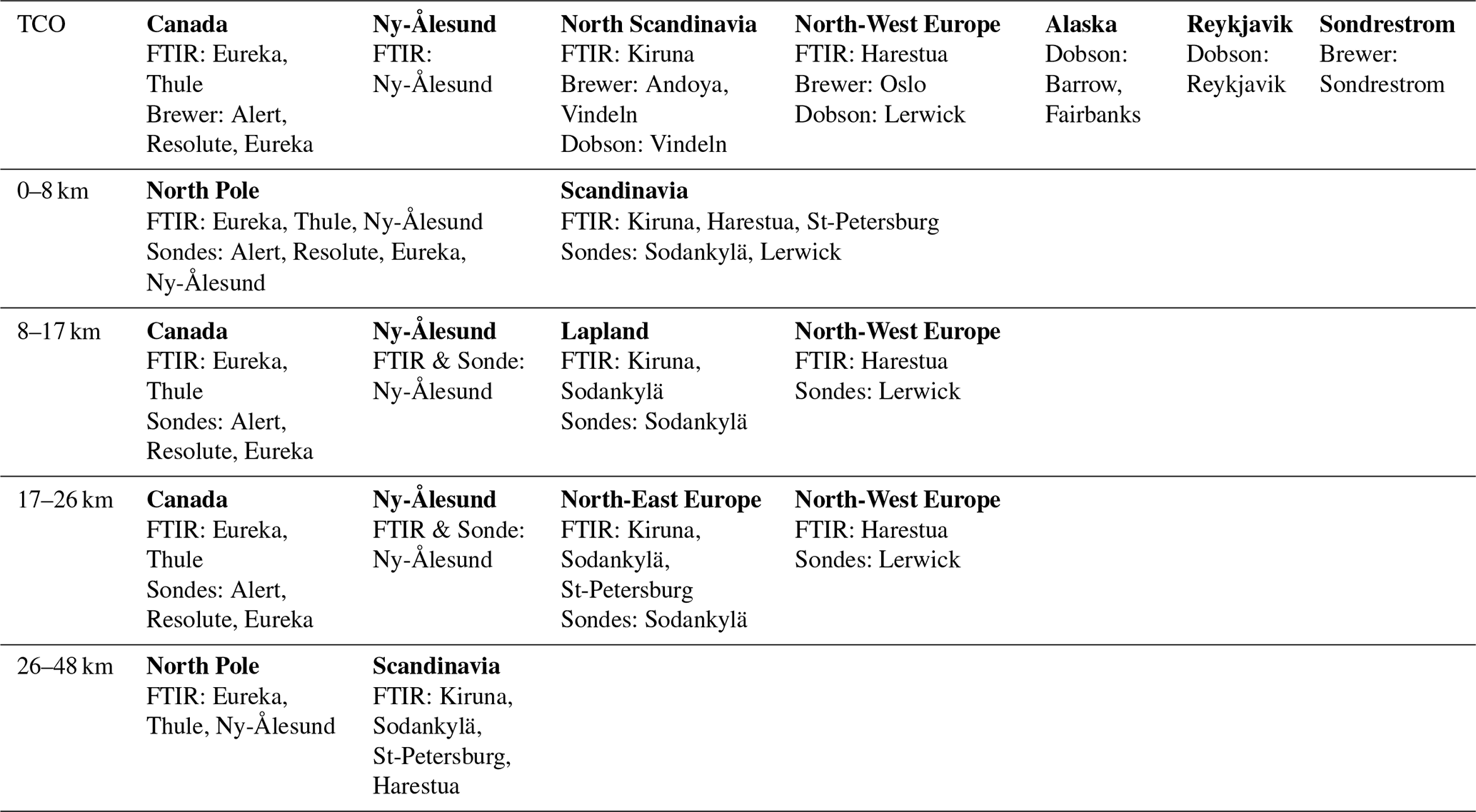
We define a group of stations as having CAMS correlation of each member station with each other member stations higher than r>0.8 (in Weatherhead et al., 2017, correlations of r>0.7 are deemed “well correlated”, while r>0.9 are “strongly correlated”). Correlations between all stations are given in Figs. A1 and A2 in Appendix A. The resulting regional groups are presented in Table 4. Some stations stand on their own and do not correlate well with any other stations. We consider them in our trend study only if their time series spans most of the 2000–2024 time period. For instance, Reykjavik and Sondrestrom in the total column are considered for trends, while St-Petersburg in the lower stratosphere and total column is not.
Table 4For each atmospheric layer, this table lists all data sets (classified by instrument) comprised in each of the groups we determined using the representativeness study and which are pictured on the maps in Fig. 11. Within a group, all station locations correlate with r>0.8, see all correlations tables in Appendix A in Figs. A1 and A2. Across layers, we have aligned groups corresponding to similar regions to represent how we can later sum partial column trends and compare with total column trends. For instance, the Canada total column trend will be compared to the sum of the North Pole tropospheric trend, the Canada lower and mid stratospheric trends and the North Pole upper stratospheric trend.
Having defined the groups of stations whose time series will be combined in order to obtain trends with reduced uncertainties, we now determine the spatial regions for which these trends will be representative. A grid-cell on the map is part of a group's region if the correlation coefficients r of the grid-cell with each of the group's stations are all larger than 0.8. If a grid-cell is part of several regional groups, the prevalence goes to the group with the highest mean of correlations between each of its stations and the grid-cell. All regional groups for each atmospheric layer are depicted in Fig. 11.
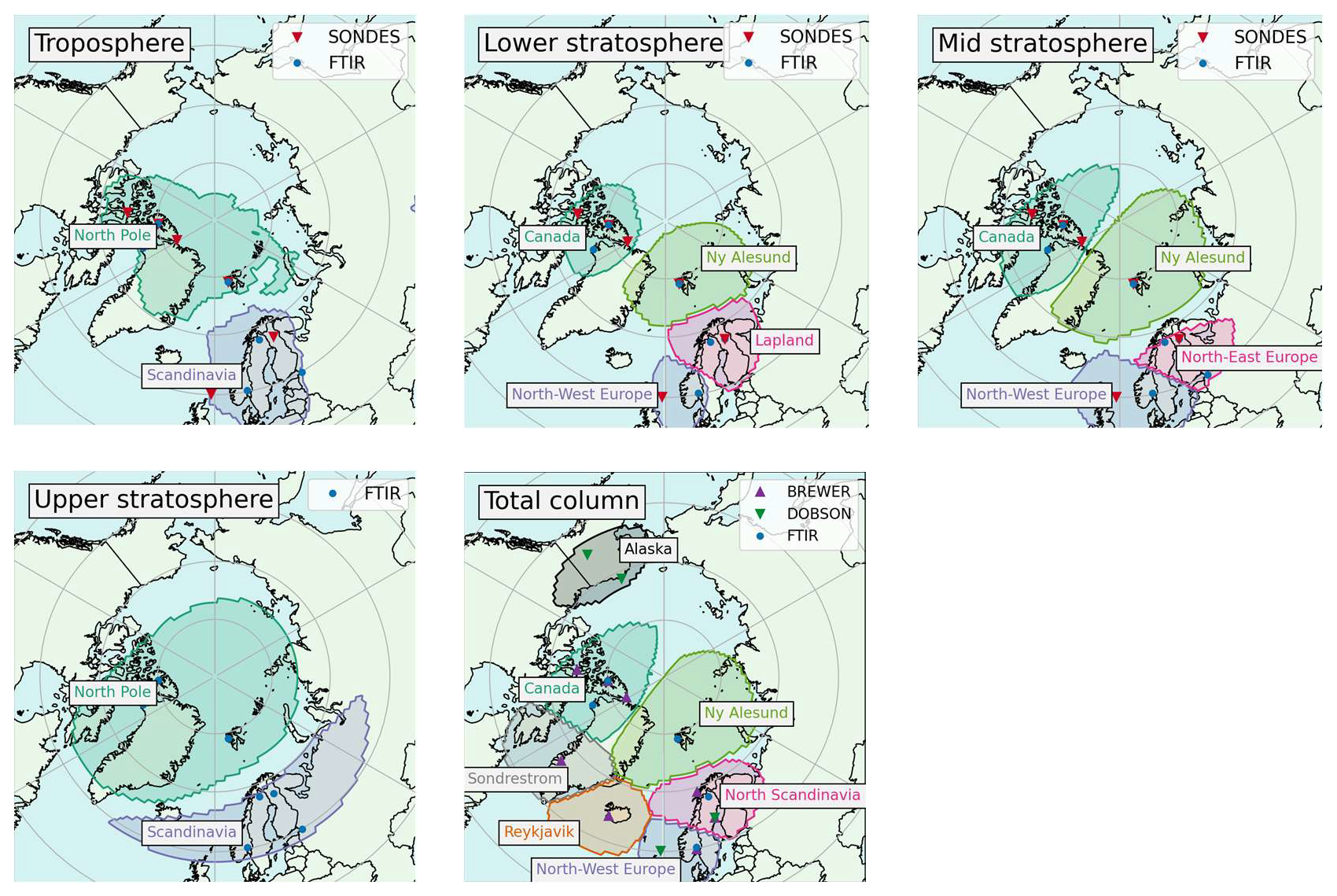
Figure 11Regional groups for the total column and each partial column, listed in Table 4. We don't consider the St-Petersburg station in the total column and the lower stratosphere because it stands on its own there but has a too short time series (2009–2024). In the upper stratosphere, Ny-Ålesund correlates equally well with Eureka and Thule as with Kiruna and Sodankylä. Since Kiruna and Sodankylä also correlate with Harestua and Lerwick, while the two latter do not correlate at all with Ny-Ålesund, we have chosen to include Ny-Ålesund with the Canadian sites.
5.1 Merged data sets
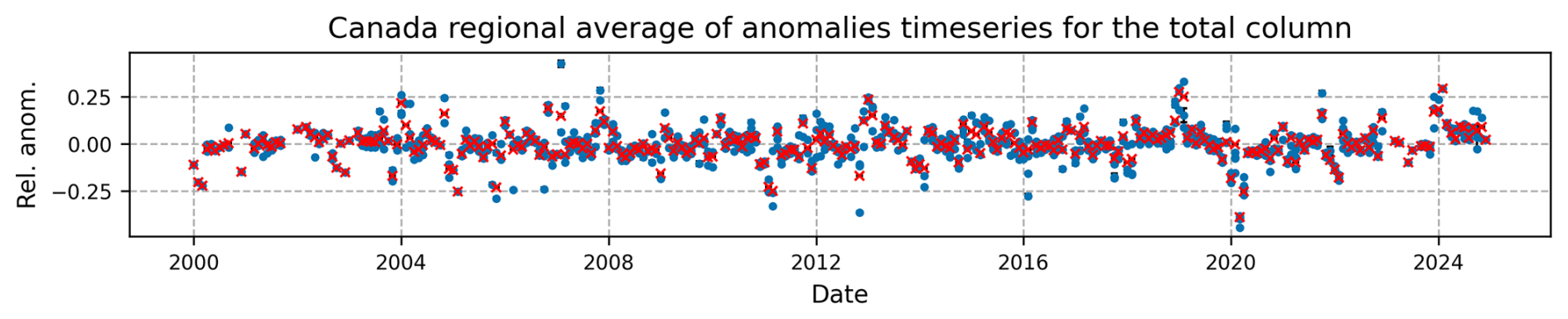
We calculate trends based on merged data sets obtained from weighted means of ozone anomalies (Eq. 1) time series, see Fig. 12 from an example with the total column anomalies of Canada. All the resulting merged data sets are available on the BIRA-IASB repository (Jonas and Vigouroux, 2026). Starting from N different anomalies data sets, anomα, their weighted merging is calculated as:
The weight used for merging is the inverse square of the anomalies errors, . Since systematic errors are affecting all values of the timeseries in the same way, we ignore them when considering anomalies and we only propagate random measurement uncertainties (considered as statistically independent) into the daily and monthly means of ozone columns and the monthly ozone anomalies. Starting from the individual measurements random uncertainties of the ozone timeseries , we calculate the uncertainties on the daily means , where Nday is the number of measurements in that specific day, and then we further propagate the random error to the monthly mean to obtain , with Nmonth the number of days of measurement within that month:
Finally, the error on the monthly relative anomalies (Eq. 1) is given by:
The random error on relative anomalies is given for each instrument and column in Table 5 in percent.
Table 5Averaged random error for anomalies for each instrument and each ozone column.
5.2 Regression model and proxies
In this section, we present the regression model and the proxies used for calculating ozone trends in the Arctic. We then analyze for each partial column the contribution of each proxies to the coefficients of determination, R2. Finally, we perform a sensitivity analysis to one of the proxies, the volume of polar stratospheric clouds.
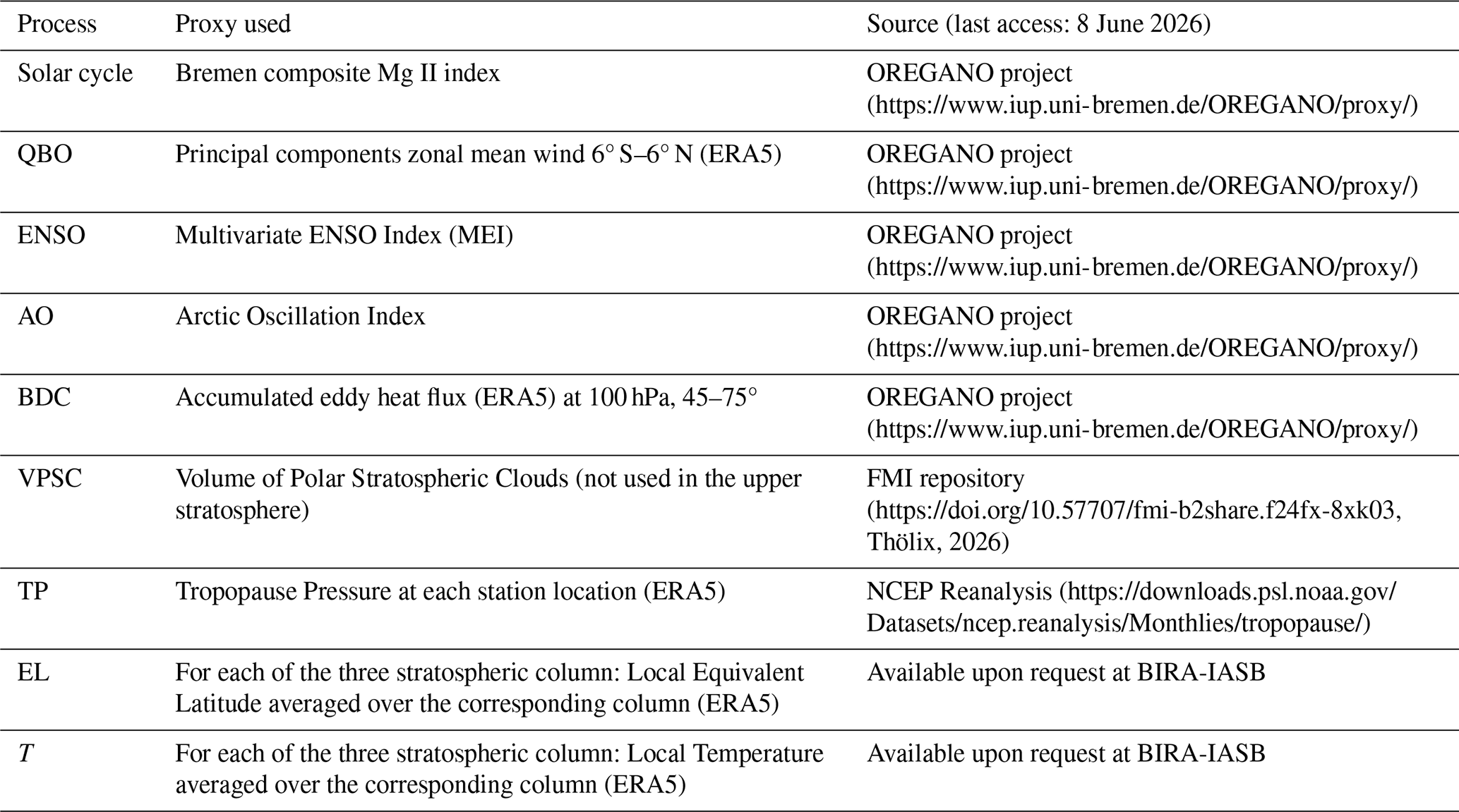
Long term trends in Arctic stratospheric ozone due to changes in ozone depleting substances are expected to be small (within a few % per decade) while the natural ozone variability is especially high in the Arctic (Brasseur and Solomon, 2005; Langematz and Tully, 2018). This means a simple linear regression is not sufficient to detect long-term trends. In this work, trends are calculated with a multiple-linear regression (MLR) using nine different proxies summarized in Table 6. These proxies try to account for the natural variability of ozone, thus reducing trends uncertainties. The proxies are similar to those used by Vigouroux et al. (2015), except that for the processes included in the LOTUS MLR model (Petropavlovskikh et al., 2019), namely Solar cycle, QBO, and ENSO, we used the LOTUS prescribed data sets made publicly available within the OREGANO project (https://www.iup.uni-bremen.de/OREGANO/proxydata/, last access: 8 June 2026). For Arctic Oscillation (AO) and Brewer-Dobson Circulation (BDC) proxies, we also use data sets provided within OREGANO, for which the accumulation during winter months has been taken into account (Weber et al., 2022). The Volume of Polar Stratospheric Clouds (VPSC) have been calculated as the volume of air between the 370 and 550 K potential temperature levels, where the temperature is below the formation temperature of ICE or NAT clouds, using ERA5 temperature (Thölix, 2026). We assumed a formation temperature of 185 K for ICE clouds and 194 K for NAT clouds (Rex et al., 2004). We also take into account the accumulation during winter, following Brunner et al. (2006). The local proxies (tropopause pressure (TP), equivalent latitude (EL) and stratospheric temperature (T)) have been taken from ERA5 reanalysis at the location of each station. Then for each region, we use as final TP, EL, and T proxies the mean of these local proxies at the sites included in a single region (Table 4). The EL and T proxies are calculated for the three stratospheric columns, leading to six proxy time series (called LS, MS, and US for the lower, middle and upper stratospheric columns, see Table 3). For each partial column, the mean of the EL (T) values in the corresponding ERA5 vertical layers is used. From all these proxies, only the local stratospheric temperature proxy is new compared to Vigouroux et al. (2015).
Thölix, 2026Table 6The nine proxies used in the MLR for attribution of ozone variability in ozone trends and their sources.
Since we use monthly anomalies (Eq. 1) for the determination of the trend, all the proxies are also deseasonalized. Note that proxies are not detrended as we want our trends to only reflect the influence of ODS changes. The effect of proxies detrending will be discussed in Sect. 5.3. For now, we model the monthly anomalies time series a(t) as:
where Xn(t) are the explanatory variables (i.e., proxies) with An their regression coefficient and A2 is the estimated trend. The trend error is given at the 2σ level and multiplied by a specific factor to account for autocorrelation (see Santer et al., 2008, which presents an alternative to the Cochrane-Orcutt method). Finally, ε(t) is the residual (difference between the regressed model and the real data). Note that the regression coefficients can be either negative or positive.
For each trend calculated, a stepwise procedure determines the relevant proxies used in the regression (Mäder et al., 2007), which can differ by region and partial column. Each of those relevant proxies adds an individual contribution Cfrac to the coefficient of determination . This individual contribution is calculated as the product of the standardized regression coefficient of the proxy with the correlation coefficient between the proxy and the observed dataset. The coefficient of determination then represents a statistical measure of the goodness of fit, i.e., how well the regressed model matches the data sets variability.
Figure 13 presents the total coefficients of determination R2 together with the individual contributions from each proxies for the annual trends in all partial columns. Similar charts for seasonal trends are shown in Fig. B1 in Appendix B.
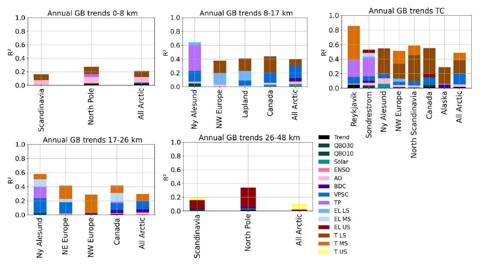
Figure 13R2 with individual contributions of proxies for all annual trends of ground-based instruments merged anomalies data sets for partial and total columns of ozone.
Note that the temperature and equivalent latitude proxies are often correlated (up to for the TLS and TMS in the total column) but thanks to the stepwise regression method, both can be included without overfitting. In cases where the stepwise procedure still selects two proxies with high correlation, we explicitly verify that their combined use positively improves the fitting of the model to the data sets (i.e., leads to a higher coefficient R2 without increasing the uncertainty on the trends). The median value of the absolute correlations between proxies is of approximately .
In all columns, the tropopause pressure (TP) doesn't contribute significantly to any of the merged regions but is relevant for the single-site regions, namely Ny-Ålesund, Reykjavik and Sondrestrom. The TP is largely influenced by the seasonal cycle and therefore strongly correlates with monthly ozone means (Hoinka et al., 1996; Steinbrecht et al., 1998), but a correlation still persists for deseasonalized anomalies (Coldewey-Egbers et al., 2022). The TP has sometimes been used as a proxy in single-site ozone trends (Vigouroux et al., 2015; Bernet et al., 2023). Because it reflects mainly local variability, in general it is not used when calculating satellite trends over zonal bands (Sofieva et al., 2021; Weber et al., 2022; Godin-Beekmann et al., 2022). The averaging of the TP time series over a region likely removes most of the correlations between ozone and TP at individual sites. However, a positive correlation between the ozone anomalies and the TP was found also for the North-Atlantic region in Coldewey-Egbers et al. (2022), so this feature may vary depending on location and region's size.
In the troposphere, the coefficients of determination for annual trends are relatively small (R2≤0.25). The main contributing proxies in the troposphere are the Arctic Oscillation (AO) and the lower stratosphere temperature (TLS), and to a smaller extent the tropopause pressure (TP) and the solar cycle (Solar). The three former can impact the troposphere via stratosphere-troposphere exchange. In this study we haven't included specific proxies to account for the tropospheric ozone variability as our main focus was on the stratosphere-troposphere exchange. Overall, tropospheric ozone variability is delicate and poorly understood. It can depend on local chemical emissions and processes (NOx, CO), forest fires, vegetation changes, as well as large-scale weather patterns. Accounting for these processes requires the use of global long-term simulations as in Law et al. (2023) and lies beyond the scope of our study.
In the lower and mid-stratospheric columns, we find that the main proxies contributing to the coefficient of determination are the equivalent latitude (EL) and the temperature (T) of the corresponding stratospheric layer. We see that the potential volume of polar stratospheric clouds is also very important except in the North-West Europe region, most probably because this region latitude is too low (about 60° N). Other proxies as the QBO, Solar cycle, ENSO, AO and BDC are present but with small contributions. The coefficients of determination R2 are of about 0.4 for merged regions and 0.6 for the single-site region of Ny-Ålesund.
In the upper stratospheric column, we find again a predominance of the equivalent latitude and temperature proxies of that layer. The R2 values are lower (0.2–0.35), with a marked diminution when considering the zonal mean (All Arctic). Note that for trends in the upper stratosphere, the VPSC proxy is not used, since polar stratospheric clouds form predominantly between 15 and 25 km of altitude.
For the total column, we find that the variability is mostly explained by the lower and mid-stratospheric temperature (TLS and TMS) and by the VPSC. As with partial columns, the AO, BDC, QBO, Solar cycle and equivalent latitudes account for smaller parts of the variability. The overall R2 values lay between 0.5–0.6, except in Reykjavik where it reaches beyond 0.8.
When analyzing contributing proxies to seasonal trends, shown in Fig. B1, we observe an overall homogeneity of proxies throughout regions, further strengthening the confidence in the results. The variability is in general best explained in spring, with R2 values about 0.7 for the total column, reasonably well explained in winter and summer, and much less well explained in autumn, especially for merged groups of several stations. This is an interesting result, as the Arctic ozone loss due to ODS is expected to be the most important during spring. The included proxies (such as VSPC which only occurs in winter and spring but also temperature and equivalent latitude) lead to better R2 values in spring, winter and summer.
The VPSC proxy has strong correlation with other proxies, in particular with the BDC (we find a correlation of −0.363 between the VPSC and the BDC proxies). A weak BDC is linked to lower temperatures and stronger vortex, and those conditions lead to more formation of PSCs (Langematz and Tully, 2018). We therefore perform a sensitivity analysis to the VPSC proxy by running the trend analysis without including this proxy. We find that part of the variability explained by the VPSC is taken up by other proxies in its absence, in majority the BDC. Both VPSC (Rex et al., 2004) and BDC proxy (Weber et al., 2011) are linked to the same dynamical phenomena and correlate strongly with polar chemical ozone loss. The QBOs, AO, TP, EL and T contributions also increase to a lesser degree. In general, about half of the variability previously explained by the VPSC is not covered up by other proxies, resulting in a coefficient of determination R2 smaller by up to 0.3 in the lower and mid-stratosphere where the effect of VPSC is the strongest. We find that adding the VPSC proxy improves our model's fit in the total column. This emphasizes the added value of using the stepwise regression, as it enables us to simultaneously use proxies with large correlations, contrary to Bernet et al. (2023) where VPSC had to be removed by hand to avoid overfitting.
5.3 Annual and seasonal trends
Before turning to the analysis of the trends results, it is important to stress that some of the proxies used in the MLR can themselves exhibit a trend. Whether or not these proxies trends should be part of the ozone trends depends on what we are trying to analyze. The VPSC for instance possesses a positive trend over the last two decades (von der Gathen et al., 2021; Pazmiño et al., 2023), which can be related to an increase of ozone depletion in the lower and mid-stratosphere. By including this proxy, together with its trend, in our MLR, we are effectively computing the ozone trend that is not due to this VPSC-related depletion. In the context of this study, this choice is justified by our aim in assessing the impact of the Montreal Protocol and its amendments, i.e., detecting the stratospheric ozone recovery associated with the diminution of ODS in the stratosphere. Therefore, our final trend results are calculated without detrending. We have nevertheless performed a sensitivity analysis by detrending each dynamical proxy (AO, BDC, VPSC, TP, EL, T) individually to assess their impact on the effective ozone levels and our conclusions. We compare trends obtained using the original proxy versus the detrended proxy, and we calculate the difference between the two. We find this difference is always non significant within the errors of the trends.
The mean absolute difference, calculated by subtracting the trend with the proxy detrended to the trend with no detrending, is of 0.80 % per decade for VPSC detrending, 0.59 % per decade for T detrending, 0.53 % per decade for EL detrending, 0.35 % per decade for AO detrending, 0.26 % per decade for BDC detrending and 0.10 % per decade for TP detrending. Although the differences are non-significant, the conclusions for very small trends such as in the lower stratosphere can be affected by those changes. First, VPSC detrending always lowers trends, leading to non-significant negative trends in the lower and mid-stratosphere. Ozone recovery above Canada in the mid-stratosphere becomes non significant when the VPSC is detrended. Note that the VPSC correlation with ozone is always negative, confirming that the correlation relies on the interannual variability and not on the trend, as expected. Temperature detrending has a smaller effect but drives the lower stratosphere trends towards negative values and the mid-stratosphere ones towards positive values. This is expected since in the polar lower stratosphere, the stratospheric cooling enhances the formation of VPSC where most of ozone-depleting reactions occurs, while on the other hand, the stratospheric cooling in mid-stratospheric altitude is associated with a slowing down of reaction rates of homogeneous chemistry, inducing a negative correlation between ozone and temperature (Barnett et al., 1975; Haigh and Pyle, 1982). EL detrending drives the trends in lower stratosphere, upper stratosphere and total column to slightly more positive trend values. AO detrending also drives lower stratospheric trends to more negative values. Finally, TP detrending drives all individual stations trends to lower and more negative values. Since we defined layers using a fixed altitude boundary, the tropopause trend (Keppens et al., 2025) also affects tropospheric and lower stratospheric ozone trends. Detailed plots illustrating these trends comparisons are shown in Fig. C1 in Appendix C, together with the trends obtained when including only the LOTUS proxies, i.e., Solar cycle, QBO and ENSO. The LOTUS trends are always smaller or more negative, because they do not include the VPSC, Temperatures and AO proxies. The uncertainties of the LOTUS trends are also always larger, making all LOTUS trends non-significant. Adding more proxies will always improve the R2 value, but it is non trivial that the uncertainty on the estimated trend is also improved, and this fact emphasizes the added value of our approach and of using more explanatory variables when calculating trends of a highly varying quantity such as ozone in the Arctic, and ensures that we are not overfitting our data.
We start by analyzing the total column trends results depicted in Fig. 14. For this and all other columns, exact numbers with the associated 2σ uncertainties, given both in % per decade and in DU per decade, are provided in Tables D1, D2 and D3 in Appendix D. We have calculated annual trends which account for the full ozone anomalies time series, as well as seasonal trends divided in winter (December–January–February), spring (March–April–May), summer (June–July–August) and autumn (September–October–November). It is important to keep in mind that due to the polar night, winter (and sometimes autumn) trends only consist of sondes profile in partial columns and of less precise measurements for Dobson and Brewer in the total column, especially at the highest latitudes where the polar night extends from October to February. We only calculate trends for time series with more than a certain number of data points (80 for annual trends and 25 for seasonal trends), so some winter or autumn trends in the total column and upper stratosphere, where only FTIR are present, are not calculated. Fewer data points during winter also implies that the variability is always larger for that season.
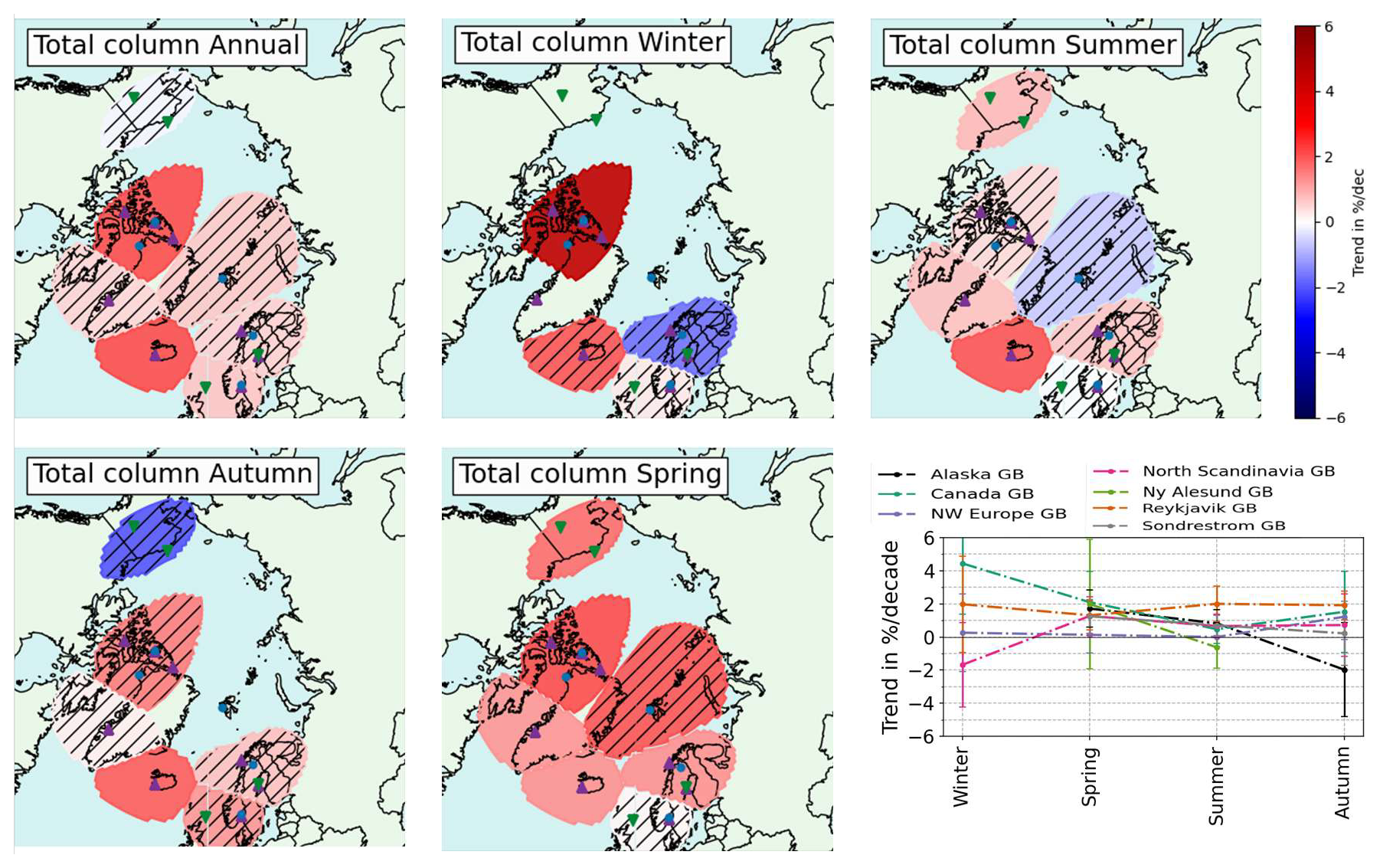
Figure 14Annual and seasonal regional trends maps for the total column of ozone. Black hatches mean the trends are not significant. Exact trend values and their 2σ uncertainties are displayed in Table D1.
In the total column, trends are found to be overall positive. Except during spring, there are some small negative trends but always non-significant. The trends in Canada, Reykjavik and Sondrestrom are always positive. The Lapland trend is negative only during winter, the Alaska one only during autumn and the Ny-Ålesund one only during summer. Many positive trends are significant, especially during spring, signalling the ozone recovery.
Previous studies of the total column of ozone in Arctic have found positive significant trends in individual stations. In Bernet et al. (2023), combined SAOZ, GUV and Brewer measurements led to annual positive significant trends at Andøya (0.9±0.7 % per decade) and Ny-Ålesund (1.5±1.0 % per decade), and a null trend at Oslo (0.1±0.5 % per decade) for the 2000–2020 period. Those values agree with our results within the 2σ uncertainties. In Anjali and Kuttippurath (2025), Arctic total column trends based on merged SAOZ, GUV, Brewer and Dobson measurements on one hand and on merged TOMS and OMI total column ozone (MSAT) data on the other hand, were found positive and significant for the 2000–2024 period in spring (respectively 0.75±0.61 and 1.04±0.85 DU yr−1), autumn (respectively 0.88±0.23 and 0.34±0.26 DU yr−1) and annually (resp. 0.65±0.39 and 0.85±0.60 DU yr−1). In order to compare with literature, we calculated Arctic zonal mean trends by merging all the Arctic ground-based stations used in this work for each partial and the total column. The results are provided in Table D1 and compare well with Anjali and Kuttippurath (2025), although based on different instruments and methodology. Finally, we point out the significant negative ozone loss trends found in Pazmiño et al. (2023) for 2000–2021 when regressing ozone loss with VPSC for the total column of ozone using chemical transport model TOMCAT/SLIMCAT, SAOZ ground-based instruments and Multi-Sensor Reanalysis (MSR2). Without the regression with VPSC, the ozone loss trend in Pazmiño et al. (2023) is not significant at the 2σ level. The VPSC detrending also lowers our total column zonal mean annual trend but it remains positive and significant (1.03±0.89 % per decade). However, our study is based on three additional years, which can accounts for the difference in significance.
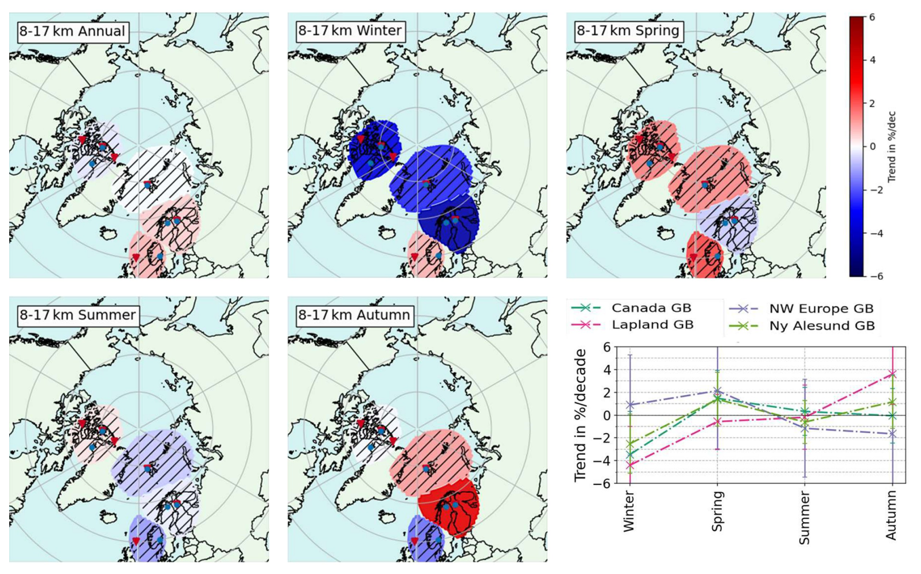
We now review all partial column trends, starting with stratospheric columns. In the lower stratospheric column (8–17 km ∼ 300–100 hPa), we find stronger seasonal and regional variations of the trends, see Fig. 15. Most trends are non-significant, and they are all very small annually. They are usually strongly negative during winter (even significantly for Lapland), and more positive during spring. Trends for Lapland are, however, positive and significant during autumn. Considering the seasonal pattern, North-West Europe distinguishes itself from other regions with positive trends in winter and negative trends in autumn, although always non-significant. As shown in Fig. C1, lower stratospheric trends become smaller or more negative when considering the detrended VPSC proxy. This indicates that the positive trend in VPSC in the Arctic is delaying the expected ozone recovery in the Arctic lower stratosphere. Trends in this layer in the Arctic are reported in Nilsen et al. (2024) for individual ozonesondes as well as in Millán et al. (2025) for two satellite data sets (ACE-FTS and MLS). The former uses Dynamical Linear Modelling (DLM) to obtain time-varying trends on 20-years periods, from 1994–2014 to 2003–2023. It considers 6 Arctic stations'sondes data sets which are also used in the present work. We do not consider their Resolute and Scoresbysund results as we found spurious jumps for those data sets in Sect. 3. At all remaining stations (Eureka, Alert, Ny-Ålesund and Sodankylä), they obtain negative annual trends within |1 % per decade| for their L2 (300–150 hPa ∼ 8–13 km) and L3 (150–40 hPa ∼ 13–22 km) layers for all periods after 1997–2017, with varying significance levels. These results agree within the 2σ errors margin. Besides our extended time-period and the addition of FTIR measurements, our analysis also differs in the proxies used for the regression. Nilsen et al. (2024) only considers the tropopause pressure, solar flux, Eddy heat flux (for the BDC) and the VPSC multiplied with Effective Equivalent Stratospheric Chlorine (EESC), which measures the impact of ozone-depleting stratospheric chlorine and bromine levels in the Arctic stratosphere. We have not included the EESC here because we want our trend term to reflect the impact of the declining ODS levels. Moreover, we found the temperature and equivalent latitude proxies (not included in their study) play a very important role in explaining the variability at these altitudes. The second study (Millán et al., 2025) reports overall positive annual trends around 2 % per decade for the MLS satellite in the 250–100 hPa layer above 60° N. These trends are not significant using a simple linear regression but become larger, positive and significant when using MLR or DLM instead. The seasonal pattern matches with ours in winter with large negative trends and in spring with more positive trends. In summer we obtain negative trends contrasting their positive trends and in autumn, we observe a strong zonal difference not captured by the latitudinal band cut of the satellite. ACE-FTS trends are highly variable (sparser sampling) but also show positive trends using MLR and DLM between 200–100 hPa in the 60–70° N latitudinal band.
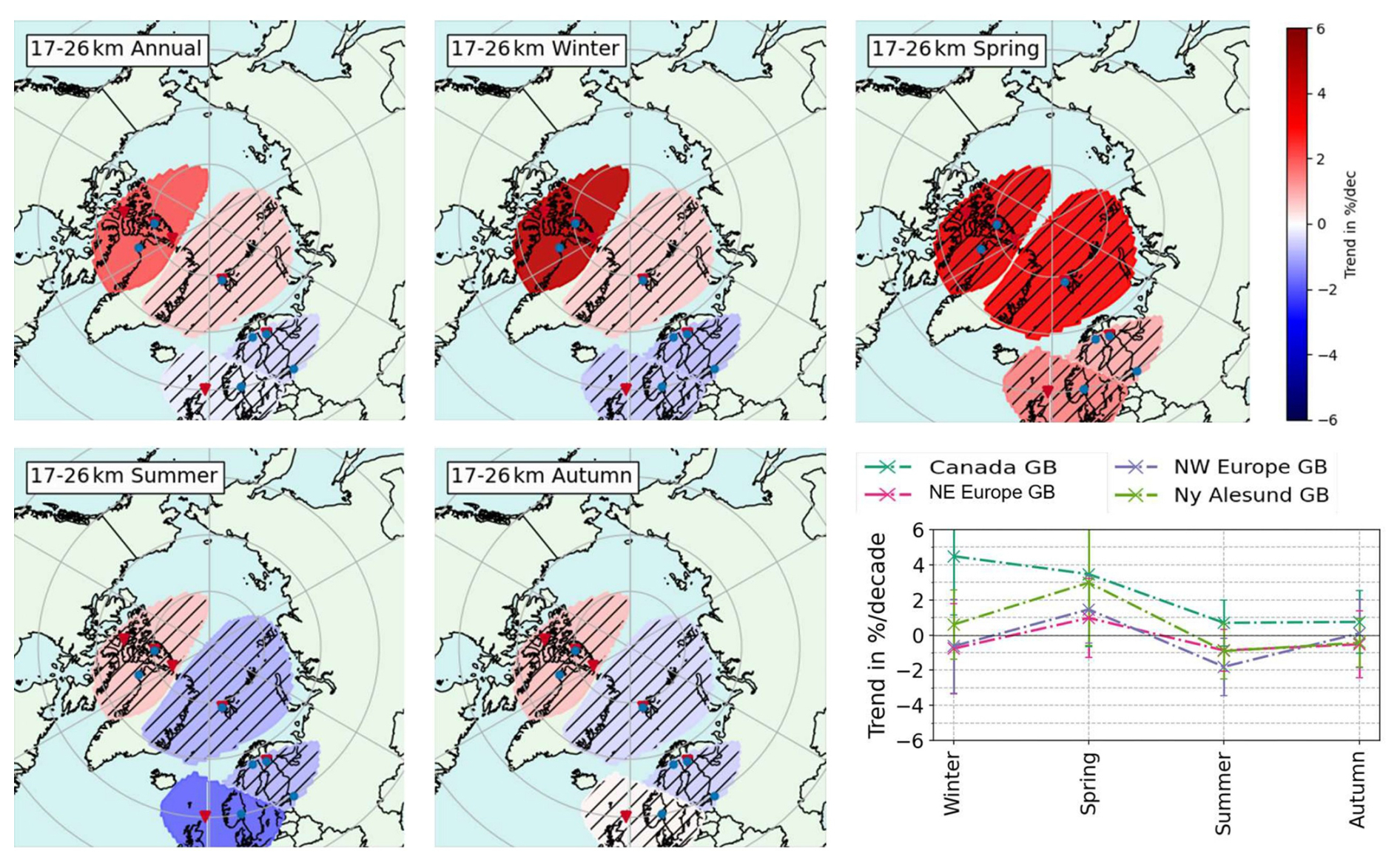
In the mid stratophere, see Fig. 16, we find positive trend values especially during spring. In Canada, trends are also positive and significant in winter and annually. There as well VPSC detrending lowers trends (see Fig. C1), highlighting that ozone recovery is delayed by this effect. In Sofieva et al. (2021), the annual trends at 20 km of altitude over the 2003–2018 period are very small on the whole region considered here, between −0.5 % per decade and +1 % per decade, but not significant anywhere. Besides, our mid-stratospheric trends exhibit a consistent seasonal cycle, with highest (positive) ozone trends during spring and lowest trends during summer (significant negative in North-West Europe). The marked zonal asymmetry between Canada and Scandinavia is discussed in the next paragraph together with the upper stratosphere.
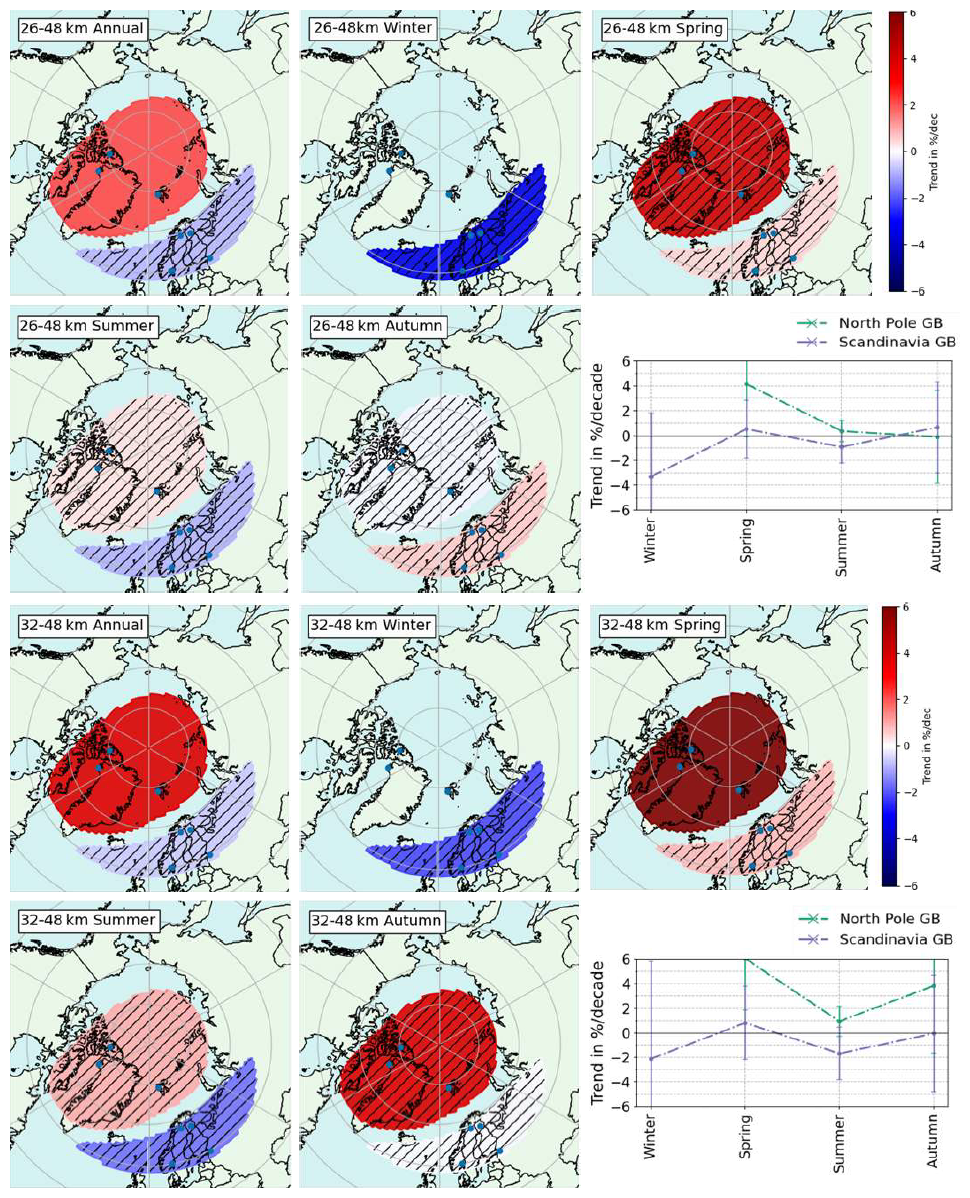
In the upper stratosphere (Fig. 17), the annual trends above North Pole are positive and significant, consistent with the results of Sofieva et al. (2021) in the 25–30 km layer and supporting the detection of ozone recovery seen in the total column trends. Seasonal trends are always non-significant, therefore we have also considered additionally the 32–48 km layer. More positive trends are generally observed at higher altitudes as in Sofieva et al. (2021) at 40 and 45 km. Indeed we find larger positive significant trends at North Pole during spring (6.06±4.19 % per decade) and annually (3.83±2.35 % per decade) for the 32–48 km layer.
In middle and upper stratosphere, we observe a zonal asymmetry as detected by satellites and models (e.g. in Arosio et al., 2019; Sofieva et al., 2021), and attributed in Arosio et al. (2024) to decadal changes in the dynamics of the polar vortex above the Arctic, stemming from climate change forcing. The zonal asymmetry is also visible when looking at which proxies are relevant: in the upper stratosphere, the North Pole trend is more influenced by the EL and the BDC, while the Scandinavian region is driven by the EL but to a lesser extent and slightly by temperature. Since the EL depends on the polar vortex, the zonal asymmetry is reduced by the use of that proxy, as it becomes larger in spring when detrending the EL. Similarly in the mid-stratosphere, the Canada region is the only one where the BDC plays a significant role, especially important in spring. This hints toward an explanation of the zonal asymmetry related to the atmospheric dynamics in the Arctic, in agreement with conclusions of Arosio et al. (2024).
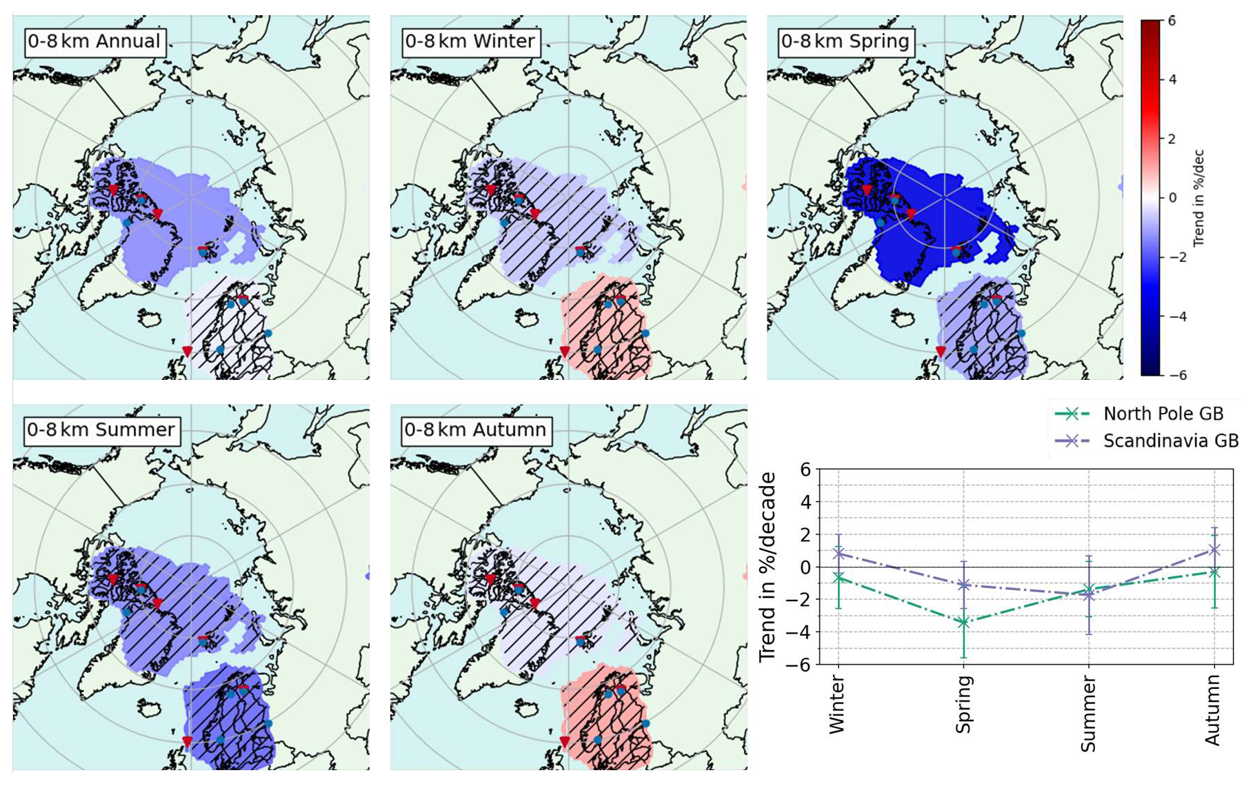
Next we consider the tropospheric ozone column in Fig. 18. We find that all tropospheric ozone trends are always negative in North Pole, significant both annually and in spring, while Scandinavian trends are always non-significant, positive in autumn and winter and negative in spring and summer. In Van Malderen et al. (2025b), the HEGIFTOM measurements using homogenized sondes, FTIR, Lidar, Umkehr and IAGOS measurements lead to merged trend results on the 2000–2022 period for the tropospheric ozone column (surf. −300 hPa) of ppb per decade in their European Arctic region and of ppb per decade in their Canadian Arctic region.1 For a tropospheric column of 8 km, we can approximate 1 DU ∼ 0.9 ppb by integrating the air density column and assuming a linear decrease of temperature in the troposphere with altitude at a rate K m−1. This approximation will be sufficient in the context of this qualitative comparison. In North Pole (Canada + Ny-Ålesund), we find a negative but smaller annual trend of ppb per decade (see Table D2 for the equivalent DU per decade trends), at the limit of agreement with Van Malderen et al. (2025b) within mutual 2σ errors. For Scandinavia we find much smaller non-significant annual trends of ppb per decade, not in agreement with the European Arctic value of Van Malderen et al. (2025b). The reasons for discrepancies are the exclusion of Scoresbysund, whose negative jump (see Sect. 3.2) drives a fake negative trend when included, the addition of two years of data and the update of FTIR data sets to the new IRWG2023 strategy. Seasonal trends results in the troposphere exhibit a clear seasonal cycle, with more negative values in spring and summer and more positive or close to zero values in autumn and winter. A similar seasonal cycle was observed in Law et al. (2023) for the 1995–2019 period, using ground-based measurements and models, but with a shift (maximum in summer). In that study, the increase in wintertime Arctic tropospheric ozone is linked to the reduction of NOx emissions in Europe and North-America mid latitudes, meaning less titration of ozone there, while the main source of tropospheric ozone at that time period comes from transports of air masses from mid to high latitudes. In the meantime, they relate the decrease in springtime tropospheric ozone to the reduction of European precursor emissions, implying less photochemical ozone production. Other factors such as the continued increase of methane or the increased dry deposition of ozone on boreal forest can also play a role.
Finally, we can compare the total column trends to the sum of all partial column trends to see how they match with each other and what is the individual contribution of each partial column to the total ozone trend (see Fig. 19 for annual and seasonal trends). We sum partial column trends in DU per decade, obtained by multiplying the trends in % per decade by the mean total column value in the corresponding region. Since regions vary across partial columns, we consider equivalent regions that we have aligned vertically in Table 4 and that we name following the smallest represented regions (those of the lower stratosphere). They are: Canada (North Pole in troposphere and upper stratosphere), Lapland (North Scandinavia in total column, Scandinavia in troposphere and upper stratosphere, North-East Europe in mid stratosphere), North-West Europe (Scandinavia in troposphere and upper stratosphere) and Ny-Ålesund (North Pole in troposphere and upper stratosphere). In addition we also show the zonal mean (All Arctic). We find that the impact of tropospheric trends is very small in DU per decade over the whole total column trend budget. Within error bars, total column trends overall agree with respective sums of partial columns trends. This is a non trivial feature since the various columns use measurements from different sets of instruments. The best match of sums of partial column trends to total column trends is observed during spring, comforting the results of ozone recovery at that season. In Ny-Ålesund in particular, the total column trend and the sum of partial columns trends agree very well both annually and for all seasons, although the upper stratospheric and total column trends are only given by the FTIR dataset while the three lower partial columns are a merging of the ozonesondes and FTIR data sets, see Table 2.
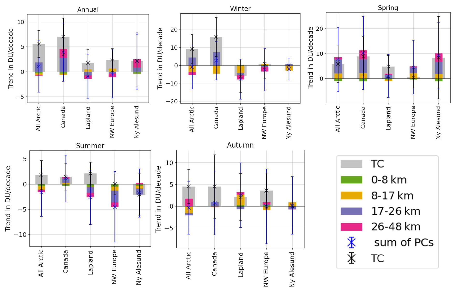
Figure 19Sums of all partial columns trends compared to total column trends in DU per decade for annual and seasonal trends. The groups are not always the same across the different layers, therefore we calculate sums for the smallest represented regions, i.e., the regions of the lower stratosphere (8–17 km). As shown in Table 4, we have for instance: Canada (TC) = North Pole (0–8 km) + Canada (8–17 km) + Canada (17–26 km) + North Pole (26–48 km) and North Scandinavia (TC) = Scandinavia (0–8 km) + Lapland (8–17 km) + North-East Europe (17–26 km) + Scandinavia (26–48 km).
By conducting a representativeness study based on CAMS re-analysis ozone profiles, we identified spatially coherent regions in which the combined time series yield reduced uncertainties and robust trend estimates for the total column as well as for four vertically resolved partial columns covering the troposphere and stratosphere (0–48 km), while enabling a finer description of ozone's evolution than zonal bands.
Cross-comparison with IASI-CDR and MEGRIDOP reveals only minor drifts (<3 % per decade) in those satellite products stratospheric columns, consistent with satellite's stability requirements (Weber, 2024), while it enabled us to exclude problematic ground-based data sets from our trend analysis. The tropospheric column of IASI is found to be slightly drifted beyond the stability requirement, so that continuous analysis is required to monitor the evolution of the drift.
Using a stepwise multiple-linear regression incorporating nine physical proxies (solar cycle, QBO, ENSO, Arctic Oscillation, Brewer–Dobson circulation, equivalent latitude, stratospheric temperature, tropopause pressure and volume of polar stratospheric clouds) we are able to detect ozone recovery (over the 2000–2024 period) due to ODS depletion while attributing ozone's variability to those physical processes. Despite the large amount of proxies used, the stepwise procedure ensures we are not overfitting, which is also verified through the improvement of fits and the reduction of trend uncertainties, visible e.g. when going from the LOTUS model to our full model. Moreover, the proxies analysis reveals a large consistency through regions, layers and seasons, giving us confidence in our trend results.
The obtained annual trends indicate a positive evolution of ozone total columns over the Arctic, statistically significant over Canada, Reykjavik (both +2.1 % per decade), and North-West Europe (+0.7 % per decade). We also detect an ozone recovery annually for the Canada region (+2 % per decade) in the mid-stratosphere (17–26 km) and for the North Pole region (Canada + Ny-Ålesund) in the upper stratosphere (+2.1 % per decade for 26–48 km and +3.8 % per decade for 32–48 km). Those trends are more pronounced during spring. Elsewhere and in the lower stratospheric column, trends are small and non-significant. Even when non significant, we see consistent seasonal patterns: e.g., trends are usually negative during winter in the lower stratosphere (significantly for Lapland), and during summer for the mid-stratosphere. The zonal asymmetry observed e.g., in Arosio et al. (2019) and Sofieva et al. (2021) for the middle and upper stratosphere is still visible in our results, despite partially accounting for it through dynamical proxies.
By analyzing the proxies influences, we find that equivalent latitude, temperature and volume of polar stratospheric clouds dominate the variability budget in stratospheric columns. The tropopause pressure plays a significant role in explaining the variability for single-site regions. We also see a slow down of the expected ozone recovery especially in the lower stratosphere (but also regionally in upper layers) due to stratospheric cooling (−0.6 % per decade) and the increase of volume of polar stratospheric clouds (−0.8 % per decade).
Annual tropospheric ozone trends are negative for the North Pole region (Canada + Ny-Ålesund), but non-significant for Scandinavia. The tropospheric trends are more negative in spring: −1.1 % per decade for Scandinavia and −3.4 % per decade (significant) for North Pole. The impact of the tropospheric trends is found to be negligible in the total column trend budget, as visible from the comparison of sums of partial columns versus total column trends.
Our study highlights the importance of long-term data sets of ozone measurements obtained simultaneously from a variety of ground-based instruments. Although ozone recovery starts to be observed in the Arctic, a continued monitoring is necessary to further assess the impact of climate change, which may undermine the efforts undertaken since the Montreal Protocol agreement, despite the successful reduction of ozone-depleting substances worldwide.
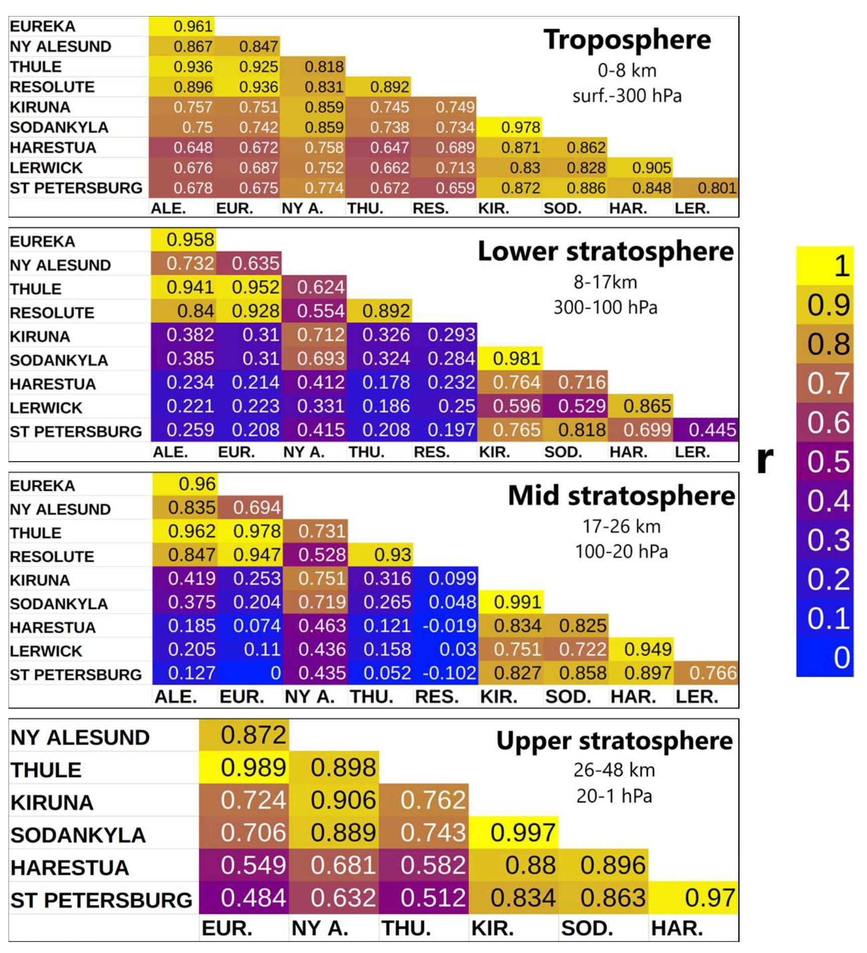
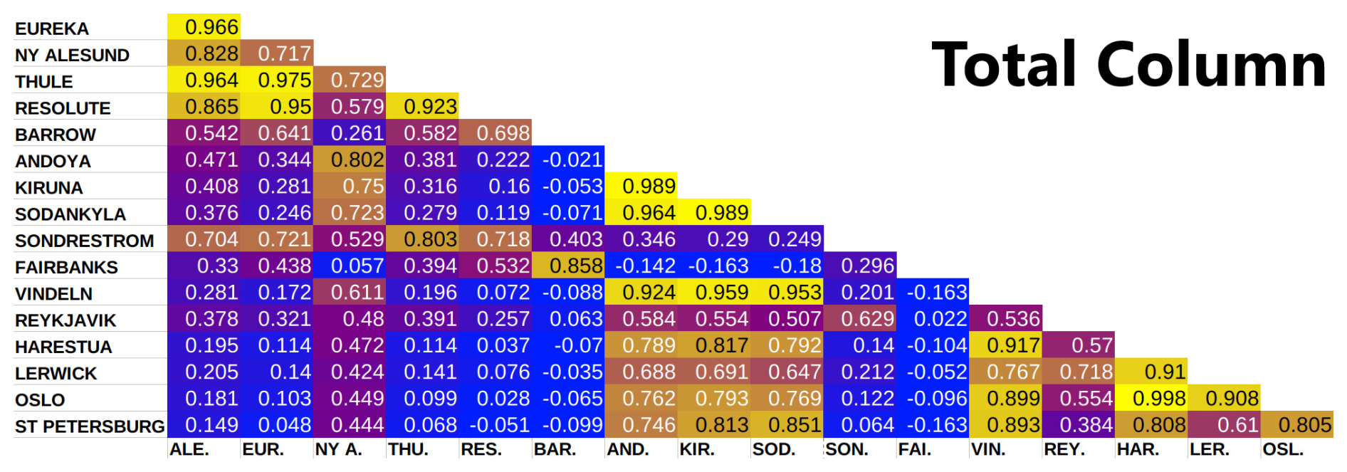
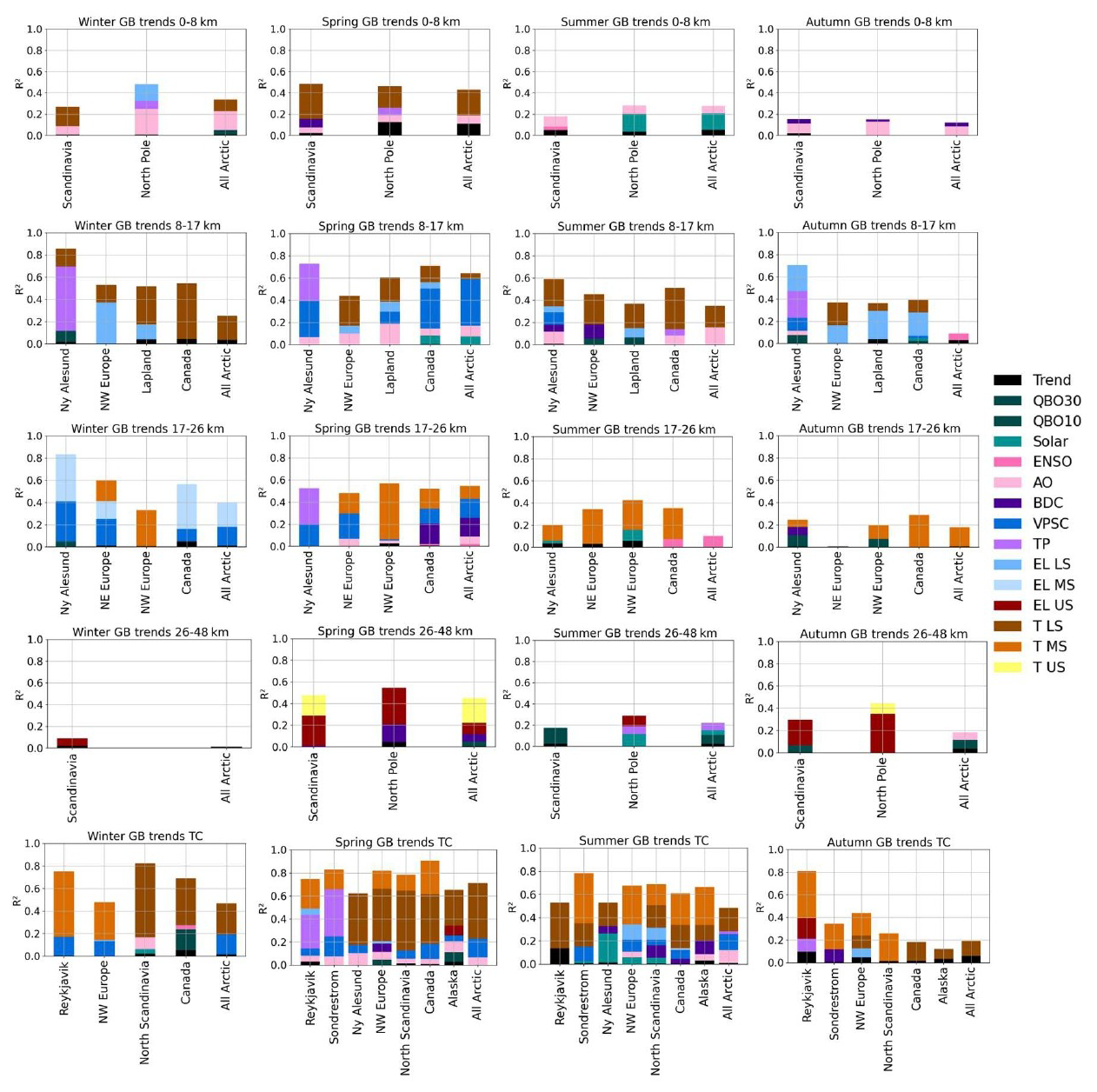
Figure B1Coefficients of determination R2 with individual contributions of proxies for all seasonal trends of ground-based instruments merged anomalies data sets.
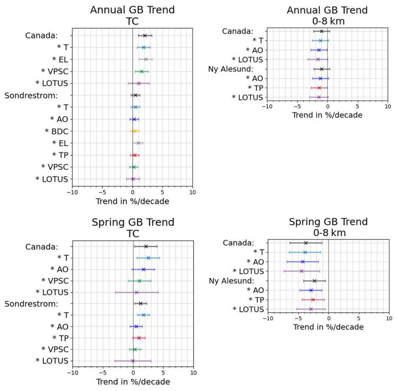
Figure C1Effect of detrending each non-LOTUS proxies on trends in Canada (a region with many merged instruments), in Sondrestrom for the total column and in Ny-Ålesund for partial columns, two single-site regions. Shown here for the total column and the troposphere. Stratospheric partial column trends are in the next figure. For each column and annual/Spring trends, we only show the detrending of proxies that are effectively contributing, to avoid unnecessary clutter. For comparison, we also show the LOTUS proxies-only trends, which always have a larger uncertainty since less variability is explained, leading to non-significant trends everywhere.
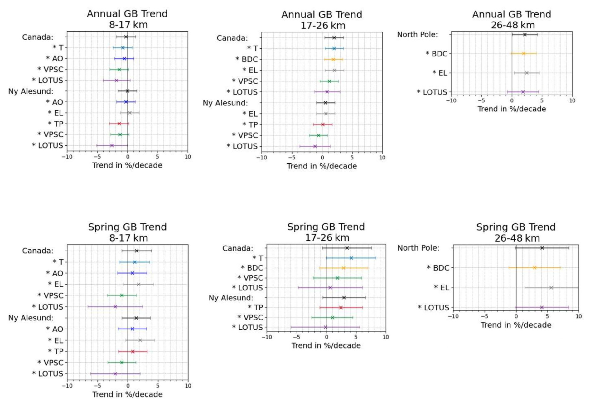
Table D1Annual and seasonal total column trends obtained from our ground-based regionally merged data sets with 2σ uncertainties, given both in percent per decade and in DU per decade. Significant trends are highlighted in bold. Missing seasons such as Ny-Ålesund winter and autumn mean that the number of available points in the time series was considered too small for applying the regression (we use a fixed threshold of at least 80 data points for annual trends and at least 25 points for seasonal trends). Partial column trends are presented in Tables D2, D3.
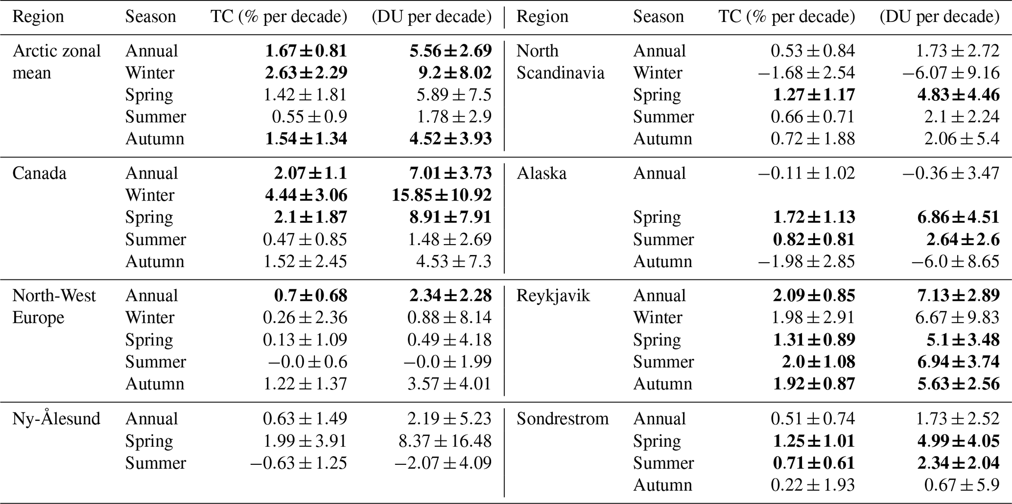
Table D2Lower and mid stratospheric regional trends in % per decade and DU per decade with 2σ uncertainties. Significant trends in bold.
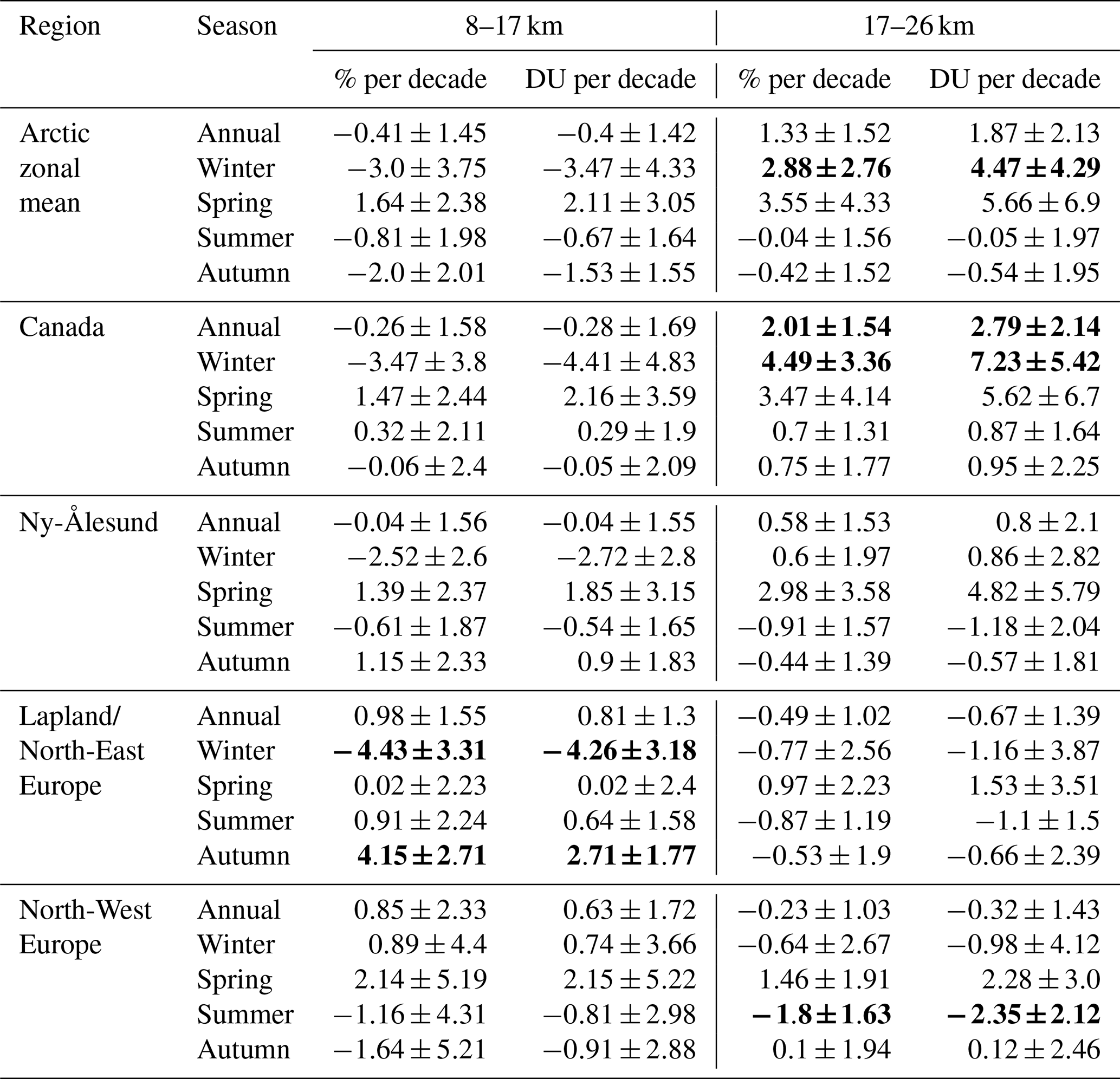
Table D3Tropospheric and upper stratospheric regional trends in % per decade and DU per decade with 2σ uncertainties. Significant trends in bold.
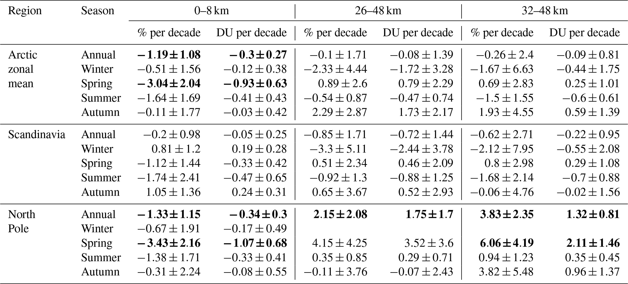
IASI-CDR: IASI is a joint mission of EUMETSAT and the Centre National d'Etudes Spatiales (CNES, France). The authors acknowledge the AERIS data infrastructure for providing access to the IASI-CDR data in this study, ULB-LATMOS for the development of the retrieval algorithms, and Eumetsat/AC SAF for O3 data production.
MEGRIDOP: Data from the European Space Agency Climate Change Initiative Ozone project, Ozone_cci (https://climate.esa.int/fr/projets/ozone/data/, Ozonecci, 2025), are provided via the BIRA archive.
The CAMS global reanalysis (EAC4) monthly averaged ozone gridded profiles used are available from the Copernicus website https://doi.org/10.24381/fd75fff2 (CAMS, 2020).
The sonde data are taken from a public ftp server, with connection details given on the HEGIFTOM website, https://hegiftom.meteo.be/datasets/tropospheric-ozone-columns-trocs (last access: 8 June 2026).
The FTIR data used in this publication are part of the Network for the Detection of Atmospheric Composition Change (NDACC) and are available through the NDACC website https://www.ndacc.org (last access: 8 June 2026), except for the Sodankylä FTIR product, available on the data repository of BIRA-IASB https://doi.org/10.18758/tzwr7tr6 (Kivi et al., 2026).
The Brewer and Dobson data are from the Ozone, World Ozone and Ultraviolet Radiation Data Centre (WOUDC), WMO/GAW Ozone Monitoring Community, World Meteorological Organization-Global Atmosphere Watch Program (WMO-GAW) https://doi.org/10.14287/10000001 (WMO/GAW Ozone Monitoring Community et al., 2013).
The merged data sets obtained from weighted means of ground-based ozone anomalies time series are available on the BIRA-IASB repository, https://doi.org/10.18758/74y0x62y (Jonas and Vigouroux, 2026).
CV designed the project. CJ, CV, and RB developed the methodologies, with the help of BL for the ozonesondes and FTIR data processing and the satellite comparison part. CJ wrote the paper, with support from CV. All other co-authors contributed to provide data sets (ground-based, satellites, or proxies) and to edit the paper.
The contact author has declared that none of the authors has any competing interests.
Publisher's note: Copernicus Publications remains neutral with regard to jurisdictional claims made in the text, published maps, institutional affiliations, or any other geographical representation in this paper. The authors bear the ultimate responsibility for providing appropriate place names. Views expressed in the text are those of the authors and do not necessarily reflect the views of the publisher.
The FTIR, Brewer, Dobson, and ozonesonde principal investigators and staff at the stations (NDACC, WOUDC) included in the work are warmly thanked for the provision of high-quality reference measurements. In particular, we thank Petra Duff and Ivan Ortega for the Eureka and Thule FTIR IRWG2023 retrievals, respectively, and Johan Mellqvist as PI of the Harestua station. Karlsruhe Institute of Technology would like to thank Uwe Raffalski from the Swedish Institute of Space Physics (IRF) and Thomas Blumenstock for their continuing support of the NDACC FTIR Kiruna activities.
VFS acknowledges support from the ESA projects OREGANO and Ozone_cci and from EU Copernicus Climate Change Service.
We thank Jenny Stavrakou and Bart Dils for useful discussions during the review of the paper. We also thank our two anonymous referees for their insightful comments and suggestions, in particular concerning the confidence in our trend results which enabled us to insist on this point in this revised version.
This research has been supported by the Belgian Federal Science Policy Office (grant no. RT/23/DORA; https://dora.aeronomie.be/, last access: 8 June 2026).
This paper was edited by Jens-Uwe Grooß and reviewed by two anonymous referees.
Anjali, S. and Kuttippurath, J.: Tracing the signatures of ozone recovery in the Arctic ozone, Sci. Rep., 15, 35304, https://doi.org/10.1038/s41598-025-19373-0, 2025. a, b, c, d
Arosio, C., Rozanov, A., Malinina, E., Weber, M., and Burrows, J. P.: Merging of ozone profiles from SCIAMACHY, OMPS and SAGE II observations to study stratospheric ozone changes, Atmos. Meas. Tech., 12, 2423–2444, https://doi.org/10.5194/amt-12-2423-2019, 2019. a, b, c
Arosio, C., Chipperfield, M. P., Rozanov, A., Weber, M., Dhomse, S., Feng, W., Jaross, G., Zhou, X., and Burrows, J. P.: Investigating Zonal Asymmetries in Stratospheric Ozone Trends From Satellite Limb Observations and a Chemical Transport Model, J. Geophys. Res.-Atmos., 129, e2023JD040353, https://doi.org/10.1029/2023JD040353, 2024. a, b
Ball, W. T., Alsing, J., Mortlock, D. J., Staehelin, J., Haigh, J. D., Peter, T., Tummon, F., Stübi, R., Stenke, A., Anderson, J., Bourassa, A., Davis, S. M., Degenstein, D., Frith, S., Froidevaux, L., Roth, C., Sofieva, V., Wang, R., Wild, J., Yu, P., Ziemke, J. R., and Rozanov, E. V.: Evidence for a continuous decline in lower stratospheric ozone offsetting ozone layer recovery, Atmos. Chem. Phys., 18, 1379–1394, https://doi.org/10.5194/acp-18-1379-2018, 2018. a
Barnett, J. J., Houghton, J. T., and Pyle, J. A.: The temperature dependence of the ozone concentration near the stratopause, Q. J. Roy. Meteor. Soc., 101, 245–257, https://doi.org/10.1002/qj.49710142808, 1975. a
Benito-Barca, S., Abalos, M., Calvo, N., Garny, H., Birner, T., Abraham, N. L., Akiyoshi, H., Dennison, F., Jöckel, P., Josse, B., Keeble, J., Kinnison, D., Marchand, M., Morgenstern, O., Plummer, D., Rozanov, E., Strode, S., Sukhodolov, T., Watanabe, S., and Yamashita, Y.: Recent Lower Stratospheric Ozone Trends in CCMI-2022 Models: Role of Natural Variability and Transport, J. Geophys. Res.-Atmos., 130, e2024JD042412, https://doi.org/10.1029/2024JD042412, 2025. a
Bernet, L., Svendby, T., Hansen, G., Orsolini, Y., Dahlback, A., Goutail, F., Pazmiño, A., Petkov, B., and Kylling, A.: Total ozone trends at three northern high-latitude stations, Atmos. Chem. Phys., 23, 4165–4184, https://doi.org/10.5194/acp-23-4165-2023, 2023. a, b, c, d, e
Björklund, R., Vigouroux, C., Effertz, P., García, O. E., Geddes, A., Hannigan, J., Miyagawa, K., Kotkamp, M., Langerock, B., Nedoluha, G., Ortega, I., Petropavlovskikh, I., Poyraz, D., Querel, R., Robinson, J., Shiona, H., Smale, D., Smale, P., Van Malderen, R., and De Mazière, M.: Intercomparison of long-term ground-based measurements of total, tropospheric, and stratospheric ozone at Lauder, New Zealand, Atmos. Meas. Tech., 17, 6819–6849, https://doi.org/10.5194/amt-17-6819-2024, 2024. a
Bontempi, G.: Statistical foundations of machine learning: the handbook, Machine Learning Group, ULB, https://leanpub.com/statisticalfoundationsofmachinelearning (last access: 8 June 2026, 2024. a
Boynard, A., Wespes, C., Hadji-Lazaro, J., Sinnathamby, S., Hurtmans, D., Coheur, P.-F., Doutriaux-Boucher, M., Onderwaater, J., Steinbrecht, W., Pennington, E. A., Bowman, K., and Clerbaux, C.: Assessment of 16-year tropospheric ozone trends from the IASI Climate Data Record, Atmos. Chem. Phys., 25, 11719–11755, https://doi.org/10.5194/acp-25-11719-2025, 2025. a, b, c, d, e, f
Brasseur, G. P. and Solomon, S.: Aeronomy of the middle atmosphere, Chemistry and Physics of the Stratosphere and Mesosphere, Atmospheric and Oceanographic Sciences Library, Springer, Dordrecht, 3rd edn., https://doi.org/10.1007/1-4020-3824-0, 2005. a, b, c
Brunner, D., Staehelin, J., Maeder, J. A., Wohltmann, I., and Bodeker, G. E.: Variability and trends in total and vertically resolved stratospheric ozone based on the CATO ozone data set, Atmos. Chem. Phys., 6, 4985–5008, https://doi.org/10.5194/acp-6-4985-2006, 2006. a
CAMS (Copernicus Atmosphere Monitoring Service): CAMS global reanalysis (EAC4) monthly averaged fields. Copernicus Atmosphere Monitoring Service (CAMS) Atmosphere Data Store [data set], https://doi.org/10.24381/fd75fff2, 2020. a
Chipperfield, M. P. and Santee, M. L.: Chapter 4: Polar Stratospheric Ozone: Past, Present, and Future, in: Scientific Assessment of Ozone Depletion: 2022, Global Ozone Research and Monitoring Project–Report No. 278, p. 509, World Meteorological Organization, Geneva, Switzerland, https://csl.noaa.gov/assessments/ozone/2022/downloads/Chapter4_2022OzoneAssessment.pdf (last access: 8 June 2026), 2022. a
Chipperfield, M. P., Dhomse, S., Hossaini, R., Feng, W., Santee, M. L., Weber, M., Burrows, J. P., Wild, J. D., Loyola, D., and Coldewey-Egbers, M.: On the Cause of Recent Variations in Lower Stratospheric Ozone, Geophys. Res. Lett., 45, 5718–5726, https://doi.org/10.1029/2018GL078071, 2018. a
Christiansen, B., Jepsen, N., Kivi, R., Hansen, G., Larsen, N., and Korsholm, U. S.: Trends and annual cycles in soundings of Arctic tropospheric ozone, Atmos. Chem. Phys., 17, 9347–9364, https://doi.org/10.5194/acp-17-9347-2017, 2017. a
Clerbaux, C. and Coheur, P.-F.: Daily IASI/Metop-A ULB-LATMOS ozone (O3) L2 product (vertical profile and columns – EUMETSAT processing), https://doi.org/10.25326/806, 2025a. a
Clerbaux, C. and Coheur, P.-F.: Daily IASI/Metop-B ULB-LATMOS ozone (O3) L2 product (vertical profile and columns – EUMETSAT processing), https://doi.org/10.25326/807, 2025b. a
Coldewey-Egbers, M., Loyola, D. G., Lerot, C., and Van Roozendael, M.: Global, regional and seasonal analysis of total ozone trends derived from the 1995–2020 GTO-ECV climate data record, Atmos. Chem. Phys., 22, 6861–6878, https://doi.org/10.5194/acp-22-6861-2022, 2022. a, b, c
Cooper, O. R., Parrish, D. D., Ziemke, J., Balashov, N. V., Cupeiro, M., Galbally, I. E., Gilge, S., Horowitz, L., Jensen, N. R., Lamarque, J.-F., Naik, V., Oltmans, S. J., Schwab, J., Shindell, D. T., Thompson, A. M., Thouret, V., Wang, Y., and Zbinden, R. M.: Global distribution and trends of tropospheric ozone: An observation-based review, Elementa, 2, https://doi.org/10.12952/journal.elementa.000029, 2014. a
De Mazière, M., Thompson, A. M., Kurylo, M. J., Wild, J. D., Bernhard, G., Blumenstock, T., Braathen, G. O., Hannigan, J. W., Lambert, J.-C., Leblanc, T., McGee, T. J., Nedoluha, G., Petropavlovskikh, I., Seckmeyer, G., Simon, P. C., Steinbrecht, W., and Strahan, S. E.: The Network for the Detection of Atmospheric Composition Change (NDACC): history, status and perspectives, Atmos. Chem. Phys., 18, 4935–4964, https://doi.org/10.5194/acp-18-4935-2018, 2018. a
Deshler, T., Stübi, R., Schmidlin, F. J., Mercer, J. L., Smit, H. G. J., Johnson, B. J., Kivi, R., and Nardi, B.: Methods to homogenize electrochemical concentration cell (ECC) ozonesonde measurements across changes in sensing solution concentration or ozonesonde manufacturer, Atmos. Meas. Tech., 10, 2021–2043, https://doi.org/10.5194/amt-10-2021-2017, 2017. a
Farman, J. C., Gardiner, B. G., and Shanklin, J. D.: Large losses of total ozone in Antarctica reveal seasonal ClOx/NOx interaction, Nature, 315, 207–210, https://doi.org/10.1038/315207a0, 1985. a
Fioletov, V., Zhao, X., Abboud, I., Brohart, M., Ogyu, A., Sit, R., Lee, S. C., Petropavlovskikh, I., Miyagawa, K., Johnson, B. J., Cullis, P., Booth, J., McConville, G., and McElroy, C. T.: Total ozone variability and trends over the South Pole during the wintertime, Atmos. Chem. Phys., 23, 12731–12751, https://doi.org/10.5194/acp-23-12731-2023, 2023. a
Fioletov, V. E., Kerr, J. B., McElroy, C. T., Wardle, D. I., Savastiouk, V., and Grajnar, T. S.: The Brewer reference triad, Geophys. Res. Lett., 32, https://doi.org/10.1029/2005GL024244, 2005. a
García, O. E., Schneider, M., Hase, F., Blumenstock, T., Sepúlveda, E., and González, Y.: Quality assessment of ozone total column amounts as monitored by ground-based solar absorption spectrometry in the near infrared (>3000 cm−1), Atmos. Meas. Tech., 7, 3071–3084, https://doi.org/10.5194/amt-7-3071-2014, 2014. a, b
Gilda, S.: tsbootstrap, Zenodo, https://doi.org/10.5281/zenodo.8226495, 2024. a
Godin-Beekmann, S., Azouz, N., Sofieva, V. F., Hubert, D., Petropavlovskikh, I., Effertz, P., Ancellet, G., Degenstein, D. A., Zawada, D., Froidevaux, L., Frith, S., Wild, J., Davis, S., Steinbrecht, W., Leblanc, T., Querel, R., Tourpali, K., Damadeo, R., Maillard Barras, E., Stübi, R., Vigouroux, C., Arosio, C., Nedoluha, G., Boyd, I., Van Malderen, R., Mahieu, E., Smale, D., and Sussmann, R.: Updated trends of the stratospheric ozone vertical distribution in the 60° S–60° N latitude range based on the LOTUS regression model , Atmos. Chem. Phys., 22, 11657–11673, https://doi.org/10.5194/acp-22-11657-2022, 2022. a
Gordon, I., Rothman, L., Hargreaves, R., Hashemi, R., Karlovets, E., Skinner, F., Conway, E., Hill, C., Kochanov, R., Tan, Y., Wcisło, P., Finenko, A., Nelson, K., Bernath, P., Birk, M., Boudon, V., Campargue, A., Chance, K., Coustenis, A., Drouin, B., Flaud, J., Gamache, R., Hodges, J., Jacquemart, D., Mlawer, E., Nikitin, A., Perevalov, V., Rotger, M., Tennyson, J., Toon, G., Tran, H., Tyuterev, V., Adkins, E., Baker, A., Barbe, A., Canè, E., Császár, A., Dudaryonok, A., Egorov, O., Fleisher, A., Fleurbaey, H., Foltynowicz, A., Furtenbacher, T., Harrison, J., Hartmann, J., Horneman, V., Huang, X., Karman, T., Karns, J., Kassi, S., Kleiner, I., Kofman, V., Kwabia-Tchana, F., Lavrentieva, N., Lee, T., Long, D., Lukashevskaya, A., Lyulin, O., Makhnev, V., Matt, W., Massie, S., Melosso, M., Mikhailenko, S., Mondelain, D., Müller, H., Naumenko, O., Perrin, A., Polyansky, O., Raddaoui, E., Raston, P., Reed, Z., Rey, M., Richard, C., Tóbiás, R., Sadiek, I., Schwenke, D., Starikova, E., Sung, K., Tamassia, F., Tashkun, S., Vander Auwera, J., Vasilenko, I., Vigasin, A., Villanueva, G., Vispoel, B., Wagner, G., Yachmenev, A., and Yurchenko, S.: The HITRAN2020 molecular spectroscopic database, J. Quant. Spectrosc. Ra., 277, 107949, https://doi.org/10.1016/j.jqsrt.2021.107949, 2022. a
Haigh, J. D. and Pyle, J. A.: Ozone perturbation experiments in a two-dimensional circulation model, Q. J. Roy. Meteor. Soc., 108, 551–574, https://doi.org/10.1002/qj.49710845705, 1982. a
Hannigan, J., Palm, M., Jones, N., Ortega, I., Langerock, B., Mahieu, E., Zhou, M., and Smale, D.: SFIT4 Line-by-line nonlinear spectral fitting software: version 1.0.18, Royal Belgian Institute for Space Aeronomy, https://doi.org/10.18758/ZEI21098, 2024. a
Harris, N. R. P., Ancellet, G., Bishop, L., Hofmann, D. J., Kerr, J. B., McPeters, R. D., Prendez, M., Randel, W. J., Staehelin, J., Subbaraya, B. H., Volz-Thomas, A., Zawodny, J., and Zerefos, C. S.: Trends in stratospheric and free tropospheric ozone, J. Geophys. Res.-Atmos., 102, 1571–1590, https://doi.org/10.1029/96JD02440, 1997. a
Hase, F., Hannigan, J., Coffey, M., Goldman, A., Höpfner, M., Jones, N., Rinsland, C., and Wood, S.: Intercomparison of retrieval codes used for the analysis of high-resolution, ground-based FTIR measurements, J. Quant. Spectrosc. Ra., 87, 25–52, https://doi.org/10.1016/j.jqsrt.2003.12.008, 2004. a
Hoinka, K. P., Claude, H., and Köhler, U.: On the correlation between tropopause pressure and ozone above central Europe, Geophys. Res. Lett., 23, 1753–1756, https://doi.org/10.1029/96GL01722, 1996. a
IASI: IASI portal, Atmospheric composition data products, https://iasi.aeris-data.fr/ (last access: 20 October 2025), 2025. a
Inness, A., Ades, M., Agustí-Panareda, A., Barré, J., Benedictow, A., Blechschmidt, A.-M., Dominguez, J. J., Engelen, R., Eskes, H., Flemming, J., Huijnen, V., Jones, L., Kipling, Z., Massart, S., Parrington, M., Peuch, V.-H., Razinger, M., Remy, S., Schulz, M., and Suttie, M.: The CAMS reanalysis of atmospheric composition, Atmos. Chem. Phys., 19, 3515–3556, https://doi.org/10.5194/acp-19-3515-2019, 2019. a, b
IRWG: Infrared Working Group, https://www2.acom.ucar.edu/irwg (last access: 17 November 2025), 2025. a, b
Jonas, C. and Vigouroux, C.: Regional weighted means of groundbased ozone (O3) anomalies timeseries in the Arctic, 2000–2024 (Version 1), Royal Belgian Institute for Space Aeronomy [data set], https://doi.org/10.18758/74y0x62y, 2026. a, b
Jonassen, M. O., Chechin, D., Karpechko, A., Lüpkes, C., Spengler, T., Tepstra, A., Vihma, T., and Zhang, X.: Dynamical Processes in the Arctic Atmosphere, 1–51, Springer International Publishing, Cham, https://doi.org/10.1007/978-3-030-33566-3_1, 2020. a
Keppens, A., Hubert, D., Granville, J., Nath, O., Lambert, J.-C., Wespes, C., Coheur, P.-F., Clerbaux, C., Boynard, A., Siddans, R., Latter, B., Kerridge, B., Di Pede, S., Veefkind, P., Cuesta, J., Dufour, G., Heue, K.-P., Coldewey-Egbers, M., Loyola, D., Orfanoz-Cheuquelaf, A., Maratt Satheesan, S., Eichmann, K.-U., Rozanov, A., Sofieva, V. F., Ziemke, J. R., Inness, A., Van Malderen, R., and Hoffmann, L.: Harmonisation of sixteen tropospheric ozone satellite data records, Atmos. Meas. Tech., 18, 6893–6916, https://doi.org/10.5194/amt-18-6893-2025, 2025. a, b
Kivi, R., Kyrö, E., Turunen, T., Harris, N. R. P., von der Gathen, P., Rex, M., Andersen, S. B., and Wohltmann, I.: Ozonesonde observations in the Arctic during 1989–2003: Ozone variability and trends in the lower stratosphere and free troposphere, J. Geophys. Res.-Atmos., 112, https://doi.org/10.1029/2006JD007271, 2007. a
Kivi, R., Vigouroux, C., Langerock, B., and Bjorklund, R.: FTIR ozone (O3) groundbased remote sensing at Sodankylä from HR125 FTS FMI instrument (Version 1), Royal Belgian Institute for Space Aeronomy [data set], https://doi.org/10.18758/tzwr7tr6, 2026. a, b
Langematz, U. and Tully, M. B.: Polar Stratospheric Ozone: Past, Present, and Future, in: Scientific Assessment of Ozone Depletion: 2018, Global Ozone Research and Monitoring Project – Report No. 58, chap. 4, World Meteorological Organization/UNEP, Geneva, Switzerland, https://wmo.int/scientific-assessment-of-ozone-depletion-2018 (last access: 2 December 2025), 2018. a, b, c
Law, K. S., Hjorth, J. L., Pernov, J. B., Whaley, C. H., Skov, H., Collaud Coen, M., Langner, J., Arnold, S. R., Tarasick, D., Christensen, J., Deushi, M., Effertz, P., Faluvegi, G., Gauss, M., Im, U., Oshima, N., Petropavlovskikh, I., Plummer, D., Tsigaridis, K., Tsyro, S., Solberg, S., and Turnock, S. T.: Arctic Tropospheric Ozone Trends, Geophys. Res. Lett., 50, e2023GL103096, https://doi.org/10.1029/2023GL103096, 2023. a, b, c
Lawrence, Z. D., Perlwitz, J., Butler, A. H., Manney, G. L., Newman, P. A., Lee, S. H., and Nash, E. R.: The Remarkably Strong Arctic Stratospheric Polar Vortex of Winter 2020: Links to Record-Breaking Arctic Oscillation and Ozone Loss, J. Geophys. Res.-Atmos., 125, e2020JD033271, https://doi.org/10.1029/2020JD033271, 2020. a
Li, Y., Dhomse, S. S., Chipperfield, M. P., Feng, W., Bian, J., Xia, Y., and Guo, D.: Quantifying stratospheric ozone trends over 1984–2020: a comparison of ordinary and regularized multivariate regression models, Atmos. Chem. Phys., 23, 13029–13047, https://doi.org/10.5194/acp-23-13029-2023, 2023. a
Mäder, J. A., Staehelin, J., Brunner, D., Stahel, W. A., Wohltmann, I., and Peter, T.: Statistical modeling of total ozone: Selection of appropriate explanatory variables, J. Geophys. Res.-Atmos., 112, https://doi.org/10.1029/2006JD007694, 2007. a, b
Millán, L., Hoor, P., Hegglin, M. I., Manney, G. L., Jeffery, P. S., Weyland, F. M., Leblanc, T., Walker, K. A., Boenisch, H., Kunkel, D., Petropavlovskikh, I., and Ye, H.: Ozone Trends in the Upper Troposphere-Lower Stratosphere Using Equivalent Latitude-Potential Temperature Coordinates, Geophys. Res. Lett., 52, e2025GL118651, https://doi.org/10.1029/2025GL118651, 2025. a, b
Nilsen, K., Kivi, R., Laine, M., Poyraz, D., Van Malderen, R., von der Gathen, P., Tarasick, D. W., Thölix, L., and Jepsen, N.: Time-varying trends from Arctic ozonesonde time series in the years 1994–2022, Sci. Rep., 14, 27683, https://doi.org/10.1038/s41598-024-75364-7, 2024. a, b, c, d, e
Okamoto, S., Ancellet, G., Godin-Beekmann, S., and Bodichon, R.: Correction of the Observatoire Haute Provence electrochemical concentration cell (ECC) ozonesonde 1991–2023 data record, Earth Syst. Sci. Data Discuss. [preprint], https://doi.org/10.5194/essd-2025-796, in review, 2026. a
Ozonecci: ESA Climate Change Initiative Ozone project, https://climate.esa.int/fr/projets/ozone/data/ (last access: 27 August 2025), 2025. a
Pazmiño, A., Goutail, F., Godin-Beekmann, S., Hauchecorne, A., Pommereau, J.-P., Chipperfield, M. P., Feng, W., Lefèvre, F., Lecouffe, A., Van Roozendael, M., Jepsen, N., Hansen, G., Kivi, R., Strong, K., and Walker, K. A.: Trends in polar ozone loss since 1989: potential sign of recovery in the Arctic ozone column, Atmos. Chem. Phys., 23, 15655–15670, https://doi.org/10.5194/acp-23-15655-2023, 2023. a, b, c, d
Petropavlovskikh, I., Godin-Beekmann, S., Hubert, D., Damadeo, R., Hassler, B., and Sofieva, V.: SPARC/IO3C/GAW Report on Long-term Ozone Trends and Uncertainties in the Stratosphere, Tech. rep., 9th assessment report of the SPARC project, International Project Office at DLR-IPA, GAW Report No. 241, WCRP Report 17/2018, https://elib.dlr.de/126666/ (last access: 8 June 2026), 2019. a, b
Rex, M., Salawitch, R. J., von der Gathen, P., Harris, N. R. P., Chipperfield, M. P., and Naujokat, B.: Arctic ozone loss and climate change, Geophys. Res. Lett., 31, https://doi.org/10.1029/2003GL018844, 2004. a, b
Rodgers, C. D.: Inverse Methods for Atmospheric Sounding, WORLD SCIENTIFIC, https://doi.org/10.1142/3171, 2000. a, b
Rodgers, C. D. and Connor, B. J.: Intercomparison of remote sounding instruments, J. Geophys. Res.-Atmos., 108, https://doi.org/10.1029/2002JD002299, 2003. a
Santer, B. D., Thorne, P. W., Haimberger, L., Taylor, K. E., Wigley, T. M. L., Lanzante, J. R., Solomon, S., Free, M., Gleckler, P. J., Jones, P. D., Karl, T. R., Klein, S. A., Mears, C., Nychka, D., Schmidt, G. A., Sherwood, S. C., and Wentz, F. J.: Consistency of modelled and observed temperature trends in the tropical troposphere, Int. J. Climatol., 28, 1703–1722, https://doi.org/10.1002/joc.1756, 2008. a
Sen, P. K.: Estimates of the Regression Coefficient Based on Kendall's Tau, J. Am. Stat. Assoc., 63, 1379–1389, 1968. a
Smit, H. and the O3S-DQA Panel: Guidelines for Homogenization of Ozonesonde Data, SI2N/O3S-DQA Activity as part of “Past Changes in the Vertical Distribution of Ozone Assessment”, https://www.wccos-josie.org/en/o3s-dqa/ (last access: 19 November 2025), 2012. a
Smit, H. G. J., Poyraz, D., Van Malderen, R., Thompson, A. M., Tarasick, D. W., Stauffer, R. M., Johnson, B. J., and Kollonige, D. E.: New insights from the Jülich Ozone Sonde Intercomparison Experiment: calibration functions traceable to one ozone reference instrument, Atmos. Meas. Tech., 17, 73–112, https://doi.org/10.5194/amt-17-73-2024, 2024. a
Smit, H. G. J., Thompson, A. M., and the ASOPOS 2.0 Panel: Ozonesonde Measurement Principles and Best Operational Practices, https://library.wmo.int/idurl/4/57720 (last access: 19 November 2025), 2021. a
Sofieva, V. F., Szeląg, M., Tamminen, J., Kyrölä, E., Degenstein, D., Roth, C., Zawada, D., Rozanov, A., Arosio, C., Burrows, J. P., Weber, M., Laeng, A., Stiller, G. P., von Clarmann, T., Froidevaux, L., Livesey, N., van Roozendael, M., and Retscher, C.: Measurement report: regional trends of stratospheric ozone evaluated using the MErged GRIdded Dataset of Ozone Profiles (MEGRIDOP), Atmos. Chem. Phys., 21, 6707–6720, https://doi.org/10.5194/acp-21-6707-2021, 2021. a, b, c, d, e, f, g, h, i
Stauffer, R. M., Thompson, A. M., Kollonige, D. E., Tarasick, D. W., Van Malderen, R., Smit, H. G. J., Vömel, H., Morris, G. A., Johnson, B. J., Cullis, P. D., Stübi, R., Davies, J., and Yan, M. M.: An Examination of the Recent Stability of Ozonesonde Global Network Data, Earth Space Sci., 9, e2022EA002459, https://doi.org/10.1029/2022EA002459, 2022. a
Steinbrecht, W., Claude, H., KöHler, U., and Hoinka, K. P.: Correlations between tropopause height and total ozone: Implications for long-term changes, J. Geophys. Res.-Atmos., 103, 19183–19192, https://doi.org/10.1029/98JD01929, 1998. a
Tarasick, D. W., Davies, J., Smit, H. G. J., and Oltmans, S. J.: A re-evaluated Canadian ozonesonde record: measurements of the vertical distribution of ozone over Canada from 1966 to 2013, Atmos. Meas. Tech., 9, 195–214, https://doi.org/10.5194/amt-9-195-2016, 2016. a, b, c
Thölix, L.: The Volume of Polar Stratospheric Clouds (VPSC), https://doi.org/10.57707/fmi-b2share.f24fx-8xk03, 2026. a, b
Van Malderen, R., Thompson, A. M., Kollonige, D. E., Stauffer, R. M., Smit, H. G. J., Maillard Barras, E., Vigouroux, C., Petropavlovskikh, I., Leblanc, T., Thouret, V., Wolff, P., Effertz, P., Tarasick, D. W., Poyraz, D., Ancellet, G., De Backer, M.-R., Evan, S., Flood, V., Frey, M. M., Hannigan, J. W., Hernandez, J. L., Iarlori, M., Johnson, B. J., Jones, N., Kivi, R., Mahieu, E., McConville, G., Müller, K., Nagahama, T., Notholt, J., Piters, A., Prats, N., Querel, R., Smale, D., Steinbrecht, W., Strong, K., and Sussmann, R.: Global ground-based tropospheric ozone measurements: reference data and individual site trends (2000–2022) from the TOAR-II/HEGIFTOM project, Atmos. Chem. Phys., 25, 7187–7225, https://doi.org/10.5194/acp-25-7187-2025, 2025a. a, b
Van Malderen, R., Zang, Z., Chang, K.-L., Björklund, R., Cooper, O. R., Liu, J., Maillard Barras, E., Vigouroux, C., Petropavlovskikh, I., Leblanc, T., Thouret, V., Wolff, P., Effertz, P., Gaudel, A., Tarasick, D. W., Smit, H. G. J., Thompson, A. M., Stauffer, R. M., Kollonige, D. E., Poyraz, D., Ancellet, G., De Backer, M.-R., Frey, M. M., Hannigan, J. W., Hernandez, J. L., Johnson, B. J., Jones, N., Kivi, R., Mahieu, E., Morino, I., McConville, G., Müller, K., Murata, I., Notholt, J., Piters, A., Prignon, M., Querel, R., Rizi, V., Smale, D., Steinbrecht, W., Strong, K., and Sussmann, R.: Ground-based tropospheric ozone measurements: regional tropospheric ozone column trends from the TOAR-II/HEGIFTOM homogenized datasets, Atmos. Chem. Phys., 25, 9905–9935, https://doi.org/10.5194/acp-25-9905-2025, 2025b. a, b, c, d, e, f, g
Vigouroux, C., De Mazière, M., Demoulin, P., Servais, C., Hase, F., Blumenstock, T., Kramer, I., Schneider, M., Mellqvist, J., Strandberg, A., Velazco, V., Notholt, J., Sussmann, R., Stremme, W., Rockmann, A., Gardiner, T., Coleman, M., and Woods, P.: Evaluation of tropospheric and stratospheric ozone trends over Western Europe from ground-based FTIR network observations, Atmos. Chem. Phys., 8, 6865–6886, https://doi.org/10.5194/acp-8-6865-2008, 2008. a
Vigouroux, C., Blumenstock, T., Coffey, M., Errera, Q., García, O., Jones, N. B., Hannigan, J. W., Hase, F., Liley, B., Mahieu, E., Mellqvist, J., Notholt, J., Palm, M., Persson, G., Schneider, M., Servais, C., Smale, D., Thölix, L., and De Mazière, M.: Trends of ozone total columns and vertical distribution from FTIR observations at eight NDACC stations around the globe, Atmos. Chem. Phys., 15, 2915–2933, https://doi.org/10.5194/acp-15-2915-2015, 2015. a, b, c, d, e, f, g, h
Vogler, C., Brönnimann, S., Staehelin, J., and Griffin, R. E. M.: Dobson total ozone series of Oxford: Reevaluation and applications, J. Geophys. Res.-Atmos., 112, https://doi.org/10.1029/2007JD008894, 2007. a
von der Gathen, P., Kivi, R., Wohltmann, I., Salawitch, R. J., and Rex, M.: Climate change favours large seasonal loss of Arctic ozone, Nat. Commun., 12, 3886, https://doi.org/10.1038/s41467-021-24089-6, 2021. a, b
Weatherhead, E. C., Bodeker, G. E., Fassò, A., Chang, K.-L., Lazo, J. K., Clack, C. T. M., Hurst, D. F., Hassler, B., English, J. M., and Yorgun, S.: Spatial Coverage of Monitoring Networks: A Climate Observing System Simulation Experiment, J. Appl. Meteorol. Clim., 56, 3211–3228, https://doi.org/10.1175/JAMC-D-17-0040.1, 2017. a, b, c
Weber, M.: Stability requirements of satellites to detect long-term stratospheric ozone trends based upon Monte Carlo simulations, Atmos. Meas. Tech., 17, 3597–3604, https://doi.org/10.5194/amt-17-3597-2024, 2024. a, b
Weber, M., Dikty, S., Burrows, J. P., Garny, H., Dameris, M., Kubin, A., Abalichin, J., and Langematz, U.: The Brewer-Dobson circulation and total ozone from seasonal to decadal time scales, Atmos. Chem. Phys., 11, 11221–11235, https://doi.org/10.5194/acp-11-11221-2011, 2011. a
Weber, M., Arosio, C., Coldewey-Egbers, M., Fioletov, V. E., Frith, S. M., Wild, J. D., Tourpali, K., Burrows, J. P., and Loyola, D.: Global total ozone recovery trends attributed to ozone-depleting substance (ODS) changes derived from five merged ozone datasets, Atmos. Chem. Phys., 22, 6843–6859, https://doi.org/10.5194/acp-22-6843-2022, 2022. a, b, c, d, e
WMO/GAW Ozone Monitoring Community, World Meteorological Organization-Global Atmosphere Watch Program (WMO-GAW), and World Ozone and Ultraviolet Radiation Data Centre (WOUDC): WMO-GAW/WOUDC Ozone and Ultraviolet Radiation Data, WOUDC [data set], https://doi.org/10.14287/10000001, 2013. a
Wohltmann, I., Rex, M., Brunner, D., and Mäder, J.: Integrated equivalent latitude as a proxy for dynamical changes in ozone column, Geophys. Res. Lett., 32, https://doi.org/10.1029/2005GL022497, 2005. a
World Meteorological Organization: Scientific Assessment of Ozone Depletion: 2022, full Report, https://library.wmo.int/idurl/4/58360 (last access: 8 June 2026), 2023. a, b, c
Zängl, G. and Hoinka, K. P.: The Tropopause in the Polar Regions, J. Climate, 14, 3117–3139, https://doi.org/10.1175/1520-0442(2001)014<3117:TTITPR>2.0.CO;2, 2001. a
Zhou, M., Wang, P., Langerock, B., Vigouroux, C., Hermans, C., Kumps, N., Wang, T., Yang, Y., Ji, D., Ran, L., Zhang, J., Xuan, Y., Chen, H., Posny, F., Duflot, V., Metzger, J.-M., and De Mazière, M.: Ground-based Fourier transform infrared (FTIR) O3 retrievals from the 3040 cm−1 spectral range at Xianghe, China, Atmos. Meas. Tech., 13, 5379–5394, https://doi.org/10.5194/amt-13-5379-2020, 2020. a, b
Note that our regions differ from those of Van Malderen et al. (2025b) because we do not consider the Scoresbysund sonde where we found a spurious drift, and we have decided to include Ny-Ålesund together with Canadian sites instead of Scandinavian ones. The correlation of Ny-Ålesund with other sites is high everywhere (0.75 annually), but when we consider seasonal correlations, we find that it correlates better with Canada in winter and spring, and better with Scandinavia in summer and autumn. This is most probably an effect of the polar vortex displacement. We have chosen to include it with Canada based on the annual correlation values.
- Abstract
- Introduction
- Ground-based data sets
- Comparison with satellite ozone data sets
- Representativeness study
- Regional trends
- Conclusions
- Appendix A: CAMS correlation tables for partial and total columns
- Appendix B: Proxies contributions to the coefficient of determination R2
- Appendix C: Comparison of trends when detrending each dynamical proxy separately
- Appendix D: Summary of all trend results for ground-based regional groups
- Data availability
- Author contributions
- Competing interests
- Disclaimer
- Acknowledgements
- Financial support
- Review statement
- References