Prognostic modeling of total specific humidity variance induced by shallow convective clouds in a GCM

Shallow convective cloud cover prediction is a critical element of climate modeling. In most global climate models (GCMs), the cloud scheme relies on a statistical description of the atmospheric water content. While the mean value of specific humidity is a standard output of the climate model, the upper moments, in particular the variance and skewness, must be prescribed by a dedicated model. Observations and large eddy simulations (LES) have shown that the asymmetry of water distribution is linked to the presence of organized convective cells. To capture this asymmetry, the boundary layer convective cells are represented in this work by an eddy diffusivity mass flux model, coupled to a bi-Gaussian statistical cloud scheme. Previously, the variance of each component has been prescribed diagnostically from the difference in specific humidity between updrafts and environment. This cloud scheme has demonstrated its capacity to represent dry shallow convective boundary layers, however, it reveals significant inaccuracies in deep convection situations and in the prediction of skewness. We propose here to develop a prognostic model for the total specific humidity variance. We show in particular that the transport of specific humidity and its square in the mass-flux scheme permits to implement the generic prognostic equations of the variance into a GCM. Furthermore, model adjustment is carried out using recently added automatic tuning methods. Based on this adjustment, we show that the prognostic model is consistent with previous work on shallow convective cases while providing significant improvements in the description of variance and third-order moment profiles.

1 Introduction

The importance of cloud representation in the radiative budget of the earth is widely documented (Bony et al., 2006; Stowasser et al., 2006; Zelinka et al., 2017) which has led climate modelers to integrate increasingly accurate cloud schemes in global climate models. Among these cloud schemes, a classical approach consists of building a sub-grid distribution of the (total or relative) humidity or of another thermodynamic quantity such as the saturation deficit (Mellor, 1977; Sommeria and Deardorff, 1977; Jam et al., 2013), which allows to characterize a saturated fraction of the mesh defining the cloud fraction. These distributions were gradually refined in their form, they were first symmetrical (triangle in Smith (1990), rectangle in Le Trent and Li (1991)) before observation and large-eddy simulations (LES) studies have shown the importance of asymmetrical distribution especially in the convective boundary layer with cumulus clouds (Lewellen and Yoh, 1993; Larson et al., 2002). Therefore it became essential to capture this asymmetry leading to various forms of the probability density functions (PDF) with non-zero skewness such as log-normal in Bony and Emanuel (2001), beta in Tompkins (2002) or bi-Gaussian distributions in Golaz et al. (2002b) or Jam et al. (2013). The modeling of the moments of the distribution has also evolved: first a priori (Smith, 1990; Le Trent and Li, 1991) then diagnosed (Bony and Emanuel, 2001; Jam et al., 2013) from thermodynamical variables or prognosed (Tompkins, 2002; Watanabe et al., 2009) with various closure hypothesis. It has been therefore necessary to develop a good understanding of the physical sources of these distribution moments, in particular to close the higher-order terms related to turbulent transport.

One approach for the determination of the moments of the subgrid water distribution in a GCM is to rely on the parameterziation of subgrid turbulent or convective transport. Most GCMs include a parametrisation of turbulent diffusion, the eddy diffusivity relying most often today on a prognostic equation of the turbulent kinetic energy (Mellor and Yamada, 1982). Whatever the sophistication of the computation of the eddy diffusivity however, this approach assumes a symmetrical distribution of turbulent motions resulting in downgradient transport. Though, alongside turbulent diffusion, the importance of convective structures carrying out non-local countergradient transport has long been established (Deardorff, 1966). In fact, this non-local transport is a key element in explaining the asymmetry of the distributions that was highlighted before. Several approaches exist to represent this non-local transport by using for example a joint bi-Gaussian PDF of velocity, liquid potential temperature and total specific humidity with higher-order closure (Golaz et al., 2002a, b; Larson et al., 2002). In this work we place ourselves within the framework of so-called mass flux schemes to represent non-local transport by organized convective plumes. The association of a mass flux scheme with a classical K-diffusion theory modeling small-scale turbulence (Mellor and Yamada, 1982; Yamada, 1983), has led to the so-called “eddy diffusivity mass flux” (EDMF) models, an idea initially proposed by Chatfield and Brost (1987), first tested by Hourdin et al. (2002) and widely disseminated since (Köhler et al., 2011; Rio and Hourdin, 2008; Pergaud et al., 2009; Neggers, 2009).

In the Laboratoire de Météorologie Dynamique atmospheric model (LMDZ), the EDMF scheme is associated with a bi-Gaussian statistical model of total specific humidity to determine cloud fraction for all clouds except those created by the deep convection scheme. The humidity variance within each Gaussian component is diagnosed from the specific humidity difference between the ascending plumes and the environment, while the asymmetry of the distribution is related to the relative weight of each Gaussian, given by the surface fraction of the updrafts. This cloud scheme has proven to be very effective in representing convective boundary layers with cloud formation at the tops of ascending plumes so as cumulus and stratocumulus clouds (Jam et al., 2013; Hourdin et al., 2019, 2021; Madeleine et al., 2020). In this scheme however, when the thermal plumes are absent or weak, the subgrid distribution reduces to a single gaussian, with a width imposed as a constant times the total water. In some cases with coexistence of shallow and deep convection, the bad representation of clouds in single columns simulations with LMDZ led us to hypothesize that the Gaussian width may be underestimated due to the omission of other sources of subgrid variance than thermal plumes as arising for instance from the detrainment of deep convection or from precipitating downdrafts. The importance of the detrainment terms of convective air masses, in particular, was demonstrated in Klein et al. (2005) (thereafter K05) based on CRM studies, after establishing the corresponding source terms in the prognostic equation of variance. Rather than adding ad-hoc diagnostic terms of variance with more free parameters, our main objective in this work is to present the implementation of K05's prognostic approach within a GCM, which has not been achieved yet. In fact K05 doubted the feasibility of implementing his developments in large-scale models because of the lack of information on the variance in the thermal plume scheme. Relying on an original methodology to circumvent this difficulties by transporting the specific humidity and its square within the thermal plume scheme, we propose here to integrate into a GCM the complete coupling of the mass flux scheme to the statistical cloud scheme via a prognostic variance equation. This approach allow us to build up a unified vision of the variance evolution and its sources with very limited free parameters. We focus here on the implementation of this prognostic model in the context of shallow convection. This first step is important to lay the theoretical and methodological foundations of the new model and to compare it to the pre-existing model and to LES in cumulus and stratocumulus scenes for which a robust tuning strategy has been developed (Couvreux et al., 2021; Hourdin et al., 2021). This tuning process employs statistical learning tools based on Bayesian inference models. The principle is to use a set of one-dimensional (1D) simulations of the model to produce a Gaussian statistical emulator of some specific metrics over the whole space of parameters. These metrics are then compared to LES simulations to determine a subspace of satisfactory parameters.

The paper is organized as follows. Section 2 presents a description of the LMDZ model setup and the methods used to develop and calibrate the prognostic parameterization, Sect. 3 presents the theoretical framework in which the prognostic model is developed, in particular the method leading to its integration into the convective transport scheme. Section 4 documents the results obtained after tuning the free parameters of the prognostic model, especially concerning cloud fraction and specific humidity variance and skewness as well as comparisons with the previous model and discussions on the different sources of variability.

2 Model and methods

In this part, we present the LMDZ model as well as the experimental methodologies and the principle of semi-automatic tuning used to calibrate and develop the prognostic physical parameterization.

2.1 The LMDZ model

The parameterization presented in this paper is tested and integrated into the global climate model of Laboratoire de Météorologie Dynamique LMDZ. LMDZ is the atmospheric component of the IPSL coupled atmosphere-ocean model, IPSL-CM, used in particular for the CMIP exercises. Concerning boundary layer subgrid scale vertical transport, LMDZ combines a K-diffusion model based on a prognostic equation of the turbulent kinetic energy (TKE) with a mass flux parameterization (Rio and Hourdin, 2008). This so-called “thermal plume model” and its coupling to a bi-Gaussian cloud scheme (Jam et al., 2013) is presented in Sect. 3.1, 3.2 and 3.3 as it is an essential element of the proposed parameterization. Deep convection on the other hand is modeled by the Emanuel's scheme (Emanuel, 1991; Emanuel and Živković-Rothman, 1999) in interaction with an original parameterization of cold pools created by reevaporation of convective rainfall (Grandpeix and Lafore, 2010; Rio et al., 2009). The LMDZ6A configuration used here, developed for CMIP6, includes developments in many aspects of the model (Madeleine et al., 2020) compared to previous CMIP5 configurations, as for example a modification of the thermal plume detrainment which led to a significant improvement of stratocumulus representation (Hourdin et al., 2019). The LMDZ model is a flexible tool which contains in particular a single column model (SCM) version. The SCM is extensively used for parameterization development, assesment and tuning based on 1D/LES comparisons.

2.2 The LES cases

The 1D/LES strategy is applied here with LES cases that embrace shallow convection scenes over earth and ocean as well as stratocumulus/cumulus transitions cases. These test cases were widely used in the development of the thermal plume model (Rio and Hourdin, 2008), the bi-Gaussian cloud scheme (Jam et al., 2013) and the modified formulation of the thermal plume detrainment (Hourdin et al., 2019). They will be refered as IHOP/REF, ARMCU/REF, RICO/REF and SANDU/REF, FAST and SLOW and we will briefly recall the context of these different 1D cases.

IHOP comes from observations carried out during the International H₂O project on 14 June 2002 on the Great Plains (Couvreux et al., 2005). It represents an almost cloudless boundary layer.

The ARM case is derived from observations collected on 21 June 1997 at the Atmospheric Radiation Measurement site in Oklahoma, USA (Brown et al., 2002). It represents a typical diurnal cycle of the shallow convective boundary layer with appearance of a few cumuli clouds in the middle of the day.

The RICO case (Rain In Cumulus over the Ocean, van Zanten et al., 2011) is a case of shallow cumuli clouds over the ocean characterized by frequent precipitation.

Finally, the SANDU REF, FAST and SLOW cases are described in Sandu and Stevens (2011). They were built by compositing the large-scale conditions encountered along a set of individual Lagrangian 3 d trajectories performed for the northeastern Pacific during the summer months of 2006 and 2007. They are meant to represent oceanic boundary layers overhung by stratocumulus clouds which become thinner with a gradual transition to shallow cumulus. REF, FAST and SLOW refer to different configurations involving more or less rapid transitions.

LES reference simulations used in this study have been performed with the MESO-NH non-hydrostatic model (Lac et al., 2018) for the IHOP, ARM and RICO cases. The LES used as a reference for the SANDU case is the one performed with the UCLA LES (Stevens and Seifert, 2008) and described in Sandu and Stevens (2011).

2.3 Model calibration

As explained in Hourdin et al. (2017), the calibration of the parameterizations of a GCM is a very sensitive step in climate modeling with the multiplication of sub-grid schemes and their associated free parameters. In LMDZ the calibration is done in successive stages from the scale of individual parameterization to the scale of the Earth's climate system as a whole. To facilitate this multi step and multi parameter tuning, automatic tuning techniques were developed (Williamson et al., 2013, 2015; Couvreux et al., 2021; Hourdin et al., 2021) based on the “history matching” approach, implemented in the “High-Tune explorer” or htexplo tool. The tool explores the model parameter space in successive waves and build an emulator of given metrics. Once this emulator is built, the parameter space is reduced at each wave according to the gap between the emulated values of the metrics and the target values of the LES. This tuning process on 1D simulations not only makes it possible to significantly reduce the parameter space but it also permits to focus and improve our understanding of the physical processes involved in the parameterizations and thus to adapt the underlying modeling work. More than a simple statistical calibration tool, it is therefore a real working support for the modeler. SCM tuning is then completed by one or several 3D waves.

Based on this approach, and using the previous mentioned 1D cases, Hourdin et al. (2021) were able to finely calibrate the key parameterizations on which we step on in the present work, the thermal plume parameterization and the cloud scheme. Here, we will reinvest the same tuning approach in order to obtain reliable and consistent comparison criteria with previous work.

3 Thermal and cloud parameterization in LMDZ

In this part, we describe the implementation of the variance prognostic model within the statistical cloud scheme. In LMDZ, the asymmetry of the total specific humidity distribution is captured by a bi-Gaussian PDF. One Gaussian is associated with the distribution within the thermal plumes and the other one within the environment of the plumes. The mass-flux scheme representing the thermal plumes and the statistical cloud scheme are therefore strongly coupled through the parameters of the PDF, and they will be even more so through the establishment of the prognostic equation of the variance. Thus, we will start this section by presenting the mass-flux parameterization of the updrafts before introducing the statistical cloud scheme, in which the specific humidity variance model is integrated.

3.1 The thermal plume model

Let ψ be a conservative variable, v the wind field and ρ the density. Using an Reynolds decomposition of the physical quantities ψ = $\stackrel{\mathrm{‾}}{\mathit{\psi }}+{\mathit{\psi }}^{\prime }$ and in the case of non-viscous transport, we can write:

$$\begin{array}{}\text{(1)}& {\displaystyle \frac{\partial \stackrel{\mathrm{‾}}{\mathit{\psi }}}{\partial t}}=-\mathit{v}\mathbf{.}\mathit{g}\mathit{r}\mathit{a}\mathit{d}\left(\stackrel{\mathrm{‾}}{\mathit{\psi }}\right)-{\displaystyle \frac{\text{div}\left(\stackrel{\mathrm{‾}}{\mathit{\rho }{w}^{\prime }{\mathit{\psi }}^{\prime }}\right)}{\mathit{\rho }}}\end{array}$$

The first term on the right-hand side is the tendency due to large-scale advection, computed by the dynamical core of the model. The second term is the tendency due to turbulent transport. It is computed in LMDZ as the sum of a K-diffusive term and a mass flux term:

$$\begin{array}{}\text{(2)}& \stackrel{\mathrm{‾}}{\mathit{\rho }{w}^{\prime }{\mathit{\psi }}^{\prime }}=-K\mathit{\rho }{\displaystyle \frac{\partial \stackrel{\mathrm{‾}}{\mathit{\psi }}}{\partial z}}+f\left(\stackrel{\mathrm{‾}}{{\mathit{\psi }}_{\mathrm{th}}}-\stackrel{\mathrm{‾}}{\mathit{\psi }}\right)\end{array}$$

The K-diffusion term follows Mellor and Yamada (1982) and includes a prognostic equation for the TKE. The mass flux transport relies on the so-called thermal plume model (Hourdin et al., 2002; Rio and Hourdin, 2008; Rio et al., 2010). It is activated only if the surface layer is unstable and relies on an original closure in Convective Availabale Potential Energy (CAPE) described by Hourdin et al. (2002). It represents a population of thermal plumes through a single equivalent thermal plume with vertical velocity $\stackrel{\mathrm{‾}}{w_{\mathrm{th}}}$ and surface fraction α. The vertical variation of the convective mass flux f = $\mathit{\rho }\mathit{\alpha }\stackrel{\mathrm{‾}}{w_{\mathrm{th}}}$, assumed stationary during one physics time step, is related to a lateral entrainment e and detrainment d through a mass conservation equation:

$$\begin{array}{}\text{(3)}& {\displaystyle \frac{\partial f}{\partial z}}=e-d\end{array}$$

The value of variable ψ within the thermal plume, noted $\stackrel{\mathrm{‾}}{{\mathit{\psi }}_{\mathrm{th}}}$, is given by the conservation equation:

$$\begin{array}{}\text{(4)}& {\displaystyle \frac{\partial f\stackrel{\mathrm{‾}}{{\mathit{\psi }}_{\mathrm{th}}}}{\partial z}}=e\stackrel{\mathrm{‾}}{\mathit{\psi }}-d\stackrel{\mathrm{‾}}{{\mathit{\psi }}_{\mathrm{th}}}+\mathit{\alpha }\mathit{\rho }S,\end{array}$$

where S is a source term for variable ψ (S ≡ 0 for a conserved variable).

The entrainment rate ϵ = $e/f$ depends positively upon the plume buoyancy B, according to the following equation:

$$\begin{array}{}\text{(5)}& \mathit{\epsilon }=max\left[\mathrm{0},{\displaystyle \frac{B\mathrm{1}}{\mathrm{1}+B\mathrm{1}}}\left({\displaystyle \frac{A\mathrm{1}B}{{\stackrel{\mathrm{‾}}{w_{\mathrm{th}}}}^{\mathrm{2}}}}-A\mathrm{2}\right)\right]\end{array}$$

where A1, B1, and A2 are tunable parameters.

The presence of parameters A1 and A2 in the computation of entrainment comes from the source term of the conservation equation for the vertical momentum (Eq. 4, with ψ = w). This source term reads S = $A\mathrm{1}B-A\mathrm{2}{\stackrel{\mathrm{‾}}{w_{\mathrm{th}}}}^{\mathrm{2}}$ and is the sum of a buoyancy and drag terms. Note that the plume fraction α is computed at each vertical level as $f/(\mathit{\rho }\stackrel{\mathrm{‾}}{w_{\mathrm{th}}}$), f being computed from the mass conservation equation and $\stackrel{\mathrm{‾}}{w_{\mathrm{th}}}$ from this vertical momentum conservation equation.

For a given value of S, the source term in the vertical momentum conservation equation, parameter B1 (taking values in [0,1]) controls whether the plume velocity increases rapidly with no lateral entrainment (B1=0) or increases less rapidly with strong lateral entrainment of air from the environment, assumed at rest (large values of B1).

The detrainment rate, δ = $d/f$, is mainly positive in the regions where the buoyancy is negative and reads

$$\begin{array}{}\text{(6)}& \mathit{\delta }=max\left[\mathrm{0},-{\displaystyle \frac{A\mathrm{1}\times B\mathrm{1}}{\mathrm{1}+B\mathrm{1}}}{\displaystyle \frac{B^{*}}{{\stackrel{\mathrm{‾}}{w_{\mathrm{th}}}}^{\mathrm{2}}}}+CQ{\left({\displaystyle \frac{\mathrm{\Delta }{q}_{\mathrm{t}}/q_{\mathrm{t}}}{{\left(\stackrel{\mathrm{‾}}{w_{\mathrm{th}}}/w_{\mathrm{0}}\right)}^{\mathrm{2}}}}\right)}^{\mathrm{0.5}}\right]\end{array}$$

with w₀ = 1 m s⁻¹. Δq_t is the contrast in humidity between the plume and its environment, and CQ is a tunable parameter. The CQ term was introduced to represent in part the enhancement of detrainment by the negative buoyancy subsequent to the evaporation of cloud water. The term is however active below the cloud as well. Note that a more physical parameterization of this CQ term is currently under development.

The computation of the buoyancy in the detrainment formulation reads:

$$\begin{array}{}\text{(7)}& B^{*}=g{\displaystyle \frac{{\mathit{\theta }}_{\mathrm{v},\mathrm{th}}\left(z\right)-{\mathit{\theta }}_{\mathrm{v}}\left(z+\mathit{\delta }z\right)}{{\mathit{\theta }}_{\mathrm{v}}(z+\mathit{\delta }z)}},\end{array}$$

where θ_v is the virtual potential temperature. In this formula, the buoyancy is computed by comparing the plume internal properties at altitude z with the environment at altitude, z + δz, with δz = DZ×z (DZ being an adjustable parameter as well). This modification enabled the thermal plume model to simulate correctly the stratocumulus and transition cases, by making the plume “aware” of the top boundary layer inversion before reaching it, thus increasing artificially detrainment just below. As explained in Hourdin et al. (2019), it may in part account for the fact that the air detrained at a given level has followed an overshoot and then a rapid downward motion, as occuring in fountains structures above stratocumulus or in so-called subsiding shells created around cumulus clouds by reevaporation of the detrained cloud water.

For the derivation of the variance model, below, we use the following Eq. (8), obtained by combining Eqs. (1) and (2) without the diffusive term:

$$\begin{array}{}\text{(8)}& {\displaystyle \frac{\partial \stackrel{\mathrm{‾}}{\mathit{\psi }}}{\partial t}}={\displaystyle \frac{d}{\mathit{\rho }}}\left(\stackrel{\mathrm{‾}}{{\mathit{\psi }}_{\mathrm{th}}}-\stackrel{\mathrm{‾}}{\mathit{\psi }}\right)+{\displaystyle \frac{f}{\mathit{\rho }}}{\displaystyle \frac{\partial \stackrel{\mathrm{‾}}{\mathit{\psi }}}{\partial z}}\end{array}$$

The first term on the right-hand is the tendency due to the thermal detrainment towards the environment, the second term is the tendency associated with the compensatory subsidence in the environment, the impact of which depends on the vertical gradient of the variable in the environment. Because the mass flux f is positive, a positive vertical gradient of the physical variable results in a positive tendency, as air with larger values of ψ is transported downward by subsidence. Here the fact that the tendency of the variable does not depend on entrainment is linked to the assumption that the entrained air is the average air of the environment. This hypothesis, which may be questioned, notably by investigating the impact of subsiding shells on the thermodynamic properties of the air in the vicinity of cumulus clouds (Heus and Jonker, 2008; Wang and Geerts, 2010; Mallaun et al., 2010), simplifies both mean and variance equation.

3.2 The cloud scheme

The LMDZ statistical cloud scheme is based on a bi-Gaussian PDF of saturation deficit in the presence of thermals (Jam et al., 2013). The saturation deficit is given by s = a_l(q_t−q_sat(T_l)) where T_l is the liquid temperature, q_t the total specific humidity, q_sat the total specific humidity at saturation and a_l is a factor depending on thermodynamic variables defined in Mellor (1977) and Sommeria and Deardorff (1977). The bi-Gaussian PDF of the deficit at saturation reads:

$$\begin{array}{}\text{(9)}& \text{PDF}\left(s\right)=(\mathrm{1}-\mathit{\alpha })\mathcal{G}\left(s,\stackrel{\mathrm{‾}}{s_{\mathrm{env}}},{\mathit{\sigma }}_{\mathrm{env}}\right)+\mathit{\alpha }\mathcal{G}\left(s,\stackrel{\mathrm{‾}}{s_{\mathrm{th}}},{\mathit{\sigma }}_{\mathrm{th}}\right),\end{array}$$

where 𝒢 is a Gaussian function of the variable s with mean value s_env and variance ${\mathit{\sigma }}_{\mathrm{env}}^{\mathrm{2}}$ in the environment and s_th and ${\mathit{\sigma }}_{\mathrm{th}}^{\mathrm{2}}$ inside the thermal plume, α being the fraction of the grid covered by the thermal plume. Because the fraction covered by thermal plumes is small (α ≪ 1) and the thermal plumes are moister than their environment (s_env < s_th), this distribution is positively skewed. We should notice that this PDF fails representing the negative asymmetry that may appear due to the presence of organised downward plumes within the compensatory subsidence. These plumes are however generally less organized than the ascending plumes forced by surface energy fluxes, and the asymmetry induced is also predominant near the surface, far from the boundary layer top where cumulus or stratocumulus clouds form.

With this choice of PDF, using the thermal plume fraction α to fix the weights of each Gaussian term, the variance and skewness of the saturation deficit are determined by the following equations being given the standard deviations σ_env and σ_th and the mean values in both environment and thermals (the detailed derivation being given in Appendix A).

$$\begin{array}{}\text{(10)}& {\displaystyle }V=\mathit{\alpha }{\mathit{\sigma }}_{\mathrm{th}}^{\mathrm{2}}+(\mathrm{1}-\mathit{\alpha }){\mathit{\sigma }}_{\mathrm{env}}^{\mathrm{2}}+\mathit{\alpha }(\mathrm{1}-\mathit{\alpha })({\stackrel{\mathrm{‾}}{s}}_{\mathrm{th}}-{\stackrel{\mathrm{‾}}{s}}_{\mathrm{env}}{)}^{\mathrm{2}}\text{(11)}& {\displaystyle }\begin{array}{rl}& S=\\ & {\displaystyle \frac{\mathrm{3}\mathit{\alpha }(\mathrm{1}-\mathit{\alpha })\left({\stackrel{\mathrm{‾}}{s}}_{\mathrm{th}}-{\stackrel{\mathrm{‾}}{s}}_{\mathrm{env}}\right)\left({\mathit{\sigma }}_{\mathrm{th}}^{\mathrm{2}}-{\mathit{\sigma }}_{\mathrm{env}}^{\mathrm{2}}\right)+\mathit{\alpha }\left(\mathrm{1}-\mathrm{3}\mathit{\alpha }+\mathrm{2}{\mathit{\alpha }}^{\mathrm{2}}\right){\left({\stackrel{\mathrm{‾}}{s}}_{\mathrm{th}}-{\stackrel{\mathrm{‾}}{s}}_{\mathrm{env}}\right)}^{\mathrm{3}}}{V^{\frac{\mathrm{3}}{\mathrm{2}}}}}\end{array}\end{array}$$

Once the PDF is given, the cloud fraction c_f of the mesh and the cloud water content q_c can be computed as:

$$\begin{array}{}\text{(12)}& {\displaystyle }{c}_{\mathrm{f}}=\underset{\mathrm{0}}{\overset{\mathrm{\infty }}{\int }}\text{PDF}\left(s\right)\mathrm{d}s\text{(13)}& {\displaystyle }{q}_{\mathrm{c}}=\underset{\mathrm{0}}{\overset{\mathrm{\infty }}{\int }}s\cdot \text{PDF}\left(s\right)\mathrm{d}s\end{array}$$

If the mean values of the saturation deficit in the updrafts and in the environment are explicitly calculated in the GCM, it remains to determine the values of the standard deviations in order to close this cloud scheme.

3.3 The original diagnostic variance model

In the current diagnostic version, the standard deviations of humidity in thermals and the environment are parameterized as follows:

$$\begin{array}{}\text{(14)}& {\mathit{\sigma }}_{\mathrm{th}}=BG\mathrm{2}(\mathit{\alpha }+\mathrm{0.01}{)}^{{\mathit{\gamma }}_{\mathrm{2}}}\left({\stackrel{\mathrm{‾}}{s}}_{\mathrm{th}}-{\stackrel{\mathrm{‾}}{s}}_{\mathrm{env}}\right)+b{\stackrel{\mathrm{‾}}{q}}_{\mathrm{th}}\end{array}$$

and

$$\begin{array}{}\text{(15)}& {\mathit{\sigma }}_{\mathrm{env}}=BG\mathrm{1}{\displaystyle \frac{{\mathit{\alpha }}^{{\mathit{\gamma }}_{\mathrm{1}}}}{\mathrm{1}-\mathit{\alpha }}}\left({\stackrel{\mathrm{‾}}{s}}_{\mathrm{th}}-{\stackrel{\mathrm{‾}}{s}}_{\mathrm{env}}\right)+b{\stackrel{\mathrm{‾}}{q}}_{\mathrm{env}}.\end{array}$$

BG1, BG2, γ₁, γ₂ and b being tunable parameters. This specific parameterization of the variance is based on a heuristic reasoning using the exchange surface and the specific humidity difference between the thermals and the environment (Jam et al., 2013). Our aim is to replace this multiparameter heuristic parameterization with a parameterization based on a well-established variance equation including all the air mass exchanges.

3.4 The variance prognostic model

Equation (8) cannot apply to the variance of a variable because the variance is not conservative. Analytical equations for the variance evolution in the presence of detraining mass fluxes have been proposed by K05 with one single plume, or by Tan et al. (2018) for a general formalism with N plumes. However their implementation in the climate model requires knowledge of the humidity variance in thermals. Although this is not an insurmountable difficulty in our model where it is predicted, we have chosen to implement a more straightforward, but theoretically equivalent, methodology consisting in transporting q and q² within the mass flux scheme. Let us first write the evolution of the variance of the total specific humidity in terms of q et q²:

$$\begin{array}{}\text{(16)}& {\displaystyle \frac{\partial \stackrel{\mathrm{‾}}{q^{\prime \mathrm{2}}}}{\partial t}}={\displaystyle \frac{\partial \stackrel{\mathrm{‾}}{q^{\mathrm{2}}}}{\partial t}}-{\displaystyle \frac{\partial {\stackrel{\mathrm{‾}}{q}}^{\mathrm{2}}}{\partial t}}={\displaystyle \frac{\partial \stackrel{\mathrm{‾}}{q^{\mathrm{2}}}}{\partial t}}-\mathrm{2}\stackrel{\mathrm{‾}}{q}{\displaystyle \frac{\partial \stackrel{\mathrm{‾}}{q}}{\partial t}}.\end{array}$$

To compute the convective variance tendency we only need knowledge of the mean total specific humidity $\stackrel{\mathrm{‾}}{q}$, its convective tendency $\frac{\partial \stackrel{\mathrm{‾}}{q}}{\partial t}$ and the convective tendency of the total specific humidity square $\frac{\partial \stackrel{\mathrm{‾}}{q^{\mathrm{2}}}}{\partial t}$. $\stackrel{\mathrm{‾}}{q}$ and $\frac{\partial \stackrel{\mathrm{‾}}{q}}{\partial t}$ are already calculated in the thermal plume model, therefore only $\frac{\partial \stackrel{\mathrm{‾}}{q^{\mathrm{2}}}}{\partial t}$ remains to be estimated. Noting that the total specific humidity is treated as a conservative variable in the thermal plume transport model, we initially assumed that its square is also conservative. Indeed, the material derivative of a squared quantity is zero if the material derivative of this quantity is zero. We would then be justified in transporting the square of the total specific humidity as a conservative tracer, just like the total specific humidity itself. However, the square is not a purely conserved quantity within the thermal plume because air parcels entering with a different humidity will mix. To subsequently account for this mixing, we added a relaxation term to the thermal plume equation.

To compute Eq. (16) in our first conservative approach (without the relaxation term) we only have to call the plume transport routine for both total humidity and its square, instead of just the first one, with no need to implement explicit equations. The consistency of this approach can be checked by deriving the analytical development which joins and provides another perspective on the K05's formalism of variance transport. Applying the Eq. (8) both to q and q², we obtain:

$$\begin{array}{}\text{(17)}& {\displaystyle \frac{\partial \stackrel{\mathrm{‾}}{q^{\prime \mathrm{2}}}}{\partial t}}={\displaystyle \frac{d}{\mathit{\rho }}}\left(\stackrel{\mathrm{‾}}{q_{\mathrm{th}}^{\mathrm{2}}}-\stackrel{\mathrm{‾}}{q^{\mathrm{2}}}\right)+{\displaystyle \frac{f}{\mathit{\rho }}}{\displaystyle \frac{\partial \stackrel{\mathrm{‾}}{q^{\mathrm{2}}}}{\partial z}}-\mathrm{2}\stackrel{\mathrm{‾}}{q}\left[{\displaystyle \frac{d}{\mathit{\rho }}}\left(\stackrel{\mathrm{‾}}{q_{\mathrm{th}}}-\stackrel{\mathrm{‾}}{q}\right)+{\displaystyle \frac{f}{\mathit{\rho }}}{\displaystyle \frac{\partial \stackrel{\mathrm{‾}}{q}}{\partial z}}\right]\end{array}$$

Subsidence terms combine as follows: $\frac{f}{\mathit{\rho }}\frac{\partial \stackrel{\mathrm{‾}}{q^{\mathrm{2}}}}{\partial z}-\mathrm{2}\stackrel{\mathrm{‾}}{q}\frac{f}{\mathit{\rho }}\frac{\partial \stackrel{\mathrm{‾}}{q}}{\partial z}=\frac{f}{\mathit{\rho }}\frac{\partial \stackrel{\mathrm{‾}}{q^{\prime \mathrm{2}}}}{\partial z}$. Detrainment terms can also be rearranged: $(\stackrel{\mathrm{‾}}{q_{\mathrm{th}}^{\mathrm{2}}}-\stackrel{\mathrm{‾}}{q^{\mathrm{2}}})-\mathrm{2}\stackrel{\mathrm{‾}}{q}(\stackrel{\mathrm{‾}}{q_{\mathrm{th}}}-\stackrel{\mathrm{‾}}{q})=(\stackrel{\mathrm{‾}}{q_{\mathrm{th}}}-\stackrel{\mathrm{‾}}{q}{)}^{\mathrm{2}}+(\stackrel{\mathrm{‾}}{q_{\mathrm{th}}^{\prime \mathrm{2}}}-\stackrel{\mathrm{‾}}{q^{\prime \mathrm{2}}})$. And the convective variance tendency finally reads:

$$\begin{array}{}\text{(18)}& {\displaystyle \frac{\partial \stackrel{\mathrm{‾}}{q^{\prime \mathrm{2}}}}{\partial t}}={\displaystyle \frac{d}{\mathit{\rho }}}\left[{\left(\stackrel{\mathrm{‾}}{q_{\mathrm{th}}}-\stackrel{\mathrm{‾}}{q}\right)}^{\mathrm{2}}+\left(\stackrel{\mathrm{‾}}{q_{\mathrm{th}}^{\prime \mathrm{2}}}-\stackrel{\mathrm{‾}}{q^{\prime \mathrm{2}}}\right)\right]+{\displaystyle \frac{f}{\mathit{\rho }}}{\displaystyle \frac{\partial \stackrel{\mathrm{‾}}{q^{\prime \mathrm{2}}}}{\partial z}}\end{array}$$

This approach leads to a similar equation that K05 derives from the mixing of two air masses and its impact on the humidity variance in the environment. This is not surprising because both approaches ultimately rely on the air mass conservation equations. In the present formalism we can underline the absence of the entrainment term, due to the already mentioned fact that we assumed that the entrained air had the average composition of the environment. We can interpret the different terms of the Eq. (18) as follows:

• The first term represents the impact of the mean values difference between the thermal plume and the environment

• The second one expresses the impact of the variances difference between the thermal plume and the environment

• The last one expresses the vertical transport of variance due to compensatory subsidence. Since the mass flux is positive, this term implies that a positive vertical gradient of variance contributes positively to the variance budget at the level considered. In physical terms, a larger variance at an upper level will tend to enhance the variance at the level below, and conversely, a smaller variance above will reduce it.

This variance transport equation is limited so far to organized convective sources which are supposed to be dominant in the studied cases, it could subsequently include however the diffusive terms, computed with the same approach by calling the diffusive transport model for both q and q². We could also include possible source/sink terms due to evaporation of precipitation for instance, or large-scale advection. This will be the subject of forthcoming publication. Here we place ourselves in a framework where the transport of variance is carried out by the organized convective terms and we only add a classical exponential dissipation term representing the small scale homogenization processes which will be discussed in Sect. 3.5. The present model finally reads:

$$\begin{array}{}\text{(19)}& {\displaystyle \frac{\partial \stackrel{\mathrm{‾}}{q^{\prime \mathrm{2}}}}{\partial t}}={\displaystyle \frac{d}{\mathit{\rho }}}\left[\right(\stackrel{\mathrm{‾}}{q_{\mathrm{th}}}-\stackrel{\mathrm{‾}}{q}{)}^{\mathrm{2}}+(\stackrel{\mathrm{‾}}{q_{\mathrm{th}}^{\prime \mathrm{2}}}-\stackrel{\mathrm{‾}}{q^{\prime \mathrm{2}}})]+{\displaystyle \frac{f}{\mathit{\rho }}}{\displaystyle \frac{\partial \stackrel{\mathrm{‾}}{q^{\prime \mathrm{2}}}}{\partial z}}-{\displaystyle \frac{\stackrel{\mathrm{‾}}{q^{\prime \mathrm{2}}}}{\mathit{\tau }}},\end{array}$$

where τ represents the relaxation time of the variance in the environment. In practice we can either implement this variance equation term by term or call the thermal transport equation for q and q² as described before. However, the two methods lead to very different implementation of the variance model, each of which having its own interest. In the first method we explicitly calculate the different terms of the Eq. (19) which allows us to compare the relative importance of this terms, especially the one associated to the difference in humidity mean and variance. The second way is simpler to implement and can be transposed to other transport processes (diffusive transport or large-scale advection for example). In this case it is no longer necessary to extract all the physical quantities from the thermal model, only the tendencies of $\stackrel{\mathrm{‾}}{q^{\mathrm{2}}}$ and $\stackrel{\mathrm{‾}}{q}$ are necessary.

As highlighted by K05, an important question underlying this theoretical approach is the determination of humidity variance in updrafts: $\stackrel{\mathrm{‾}}{q_{\mathrm{th}}^{\prime \mathrm{2}}}$. In the diagnostic parameterization, it was prescribed using the humidity difference with the environment. However, the transport of q and q² within the thermal model now gives us direct access to $\stackrel{\mathrm{‾}}{q_{\mathrm{th}}^{\prime \mathrm{2}}}$ = $\stackrel{\mathrm{‾}}{q_{\mathrm{th}}^{\mathrm{2}}}-{\stackrel{\mathrm{‾}}{q_{\mathrm{th}}}}^{\mathrm{2}}$.

With the same algebra as above, starting from the Eq. (4) applied to q_th and $q_{\mathrm{th}}^{\mathrm{2}}$, we obtain the following expression for the vertical evolution of the variance in the thermal.

$$\begin{array}{}\text{(20)}& {\displaystyle \frac{\partial \stackrel{\mathrm{‾}}{q_{\mathrm{th}}^{\prime \mathrm{2}}}}{\partial z}}=\mathit{ϵ}\left[{\left(\stackrel{\mathrm{‾}}{q_{\mathrm{th}}}-\stackrel{\mathrm{‾}}{q}\right)}^{\mathrm{2}}+\left(\stackrel{\mathrm{‾}}{q^{\prime \mathrm{2}}}-\stackrel{\mathrm{‾}}{q_{\mathrm{th}}^{\prime \mathrm{2}}}\right)\right]\end{array}$$

when considering q² as a conserved quantity. This expression can be completed by a relaxation term representing small-scale diffusion processes in the thermal. The advective-diffusive coupling leads to the introduction of a characteristic diffusion height z₀ = $\stackrel{\mathrm{‾}}{w_{\mathrm{th}}}{\mathit{\tau }}_{\mathrm{th}}$ in the thermal plume where $\stackrel{\mathrm{‾}}{w_{\mathrm{th}}}$ is the vertical advection and τ_th the diffusion timescale in the plume.

$$\begin{array}{}\text{(21)}& {\displaystyle \frac{\partial \stackrel{\mathrm{‾}}{q_{\mathrm{th}}^{\prime \mathrm{2}}}}{\partial z}}=\mathit{ϵ}\left[{\left(\stackrel{\mathrm{‾}}{q}-\stackrel{\mathrm{‾}}{q_{\mathrm{th}}}\right)}^{\mathrm{2}}+\left(\stackrel{\mathrm{‾}}{q^{\prime \mathrm{2}}}-\stackrel{\mathrm{‾}}{q_{\mathrm{th}}^{\prime \mathrm{2}}}\right)\right]-{\displaystyle \frac{\stackrel{\mathrm{‾}}{q_{\mathrm{th}}^{\prime \mathrm{2}}}}{\stackrel{\mathrm{‾}}{w_{\mathrm{th}}}{\mathit{\tau }}_{\mathrm{th}}}}\end{array}$$

In practice, $q_{\mathrm{th}}^{\prime \mathrm{2}}$ can be computed applying the thermal plume model to q² instead of q, adding the relaxation term in the computation, which requires to provide the value of q_th obtained in the transport computation of q by the thermal plume model.

3.5 The relaxation time in the variance model

The Newton relaxation time τ which appears in the dissipation term is an important parameter of the variance calculation. It can be estimated as the relaxation time of the turbulent energy as was proposed in Nieuwstadt and Brost (1986) and Neggers (2009). Tompkins (2002) proposes to add to this small-scale relaxation a second dissipation process associated with slower large-scale two-dimensional (2D) dissipation due to horizontal wind shear instability. This second component would be present even in case of strong temperature stratification. Although it will be a part of our reflection when extending our work to the upper atmosphere, we neglect it here, as we only focus on shallow convective cases where the first component is expected to be dominant. The order of magnitude of the turbulence relaxation time is:

$$\begin{array}{}\text{(22)}& \mathit{\tau }={\displaystyle \frac{l}{\sqrt{\text{TKE}}}}\end{array}$$

l being a mixing length of roughly 100 m (Blackadar, 1962). We obtain an order of magnitude of 100 to 1000 s for τ which is a fairly fast relaxation, especially compared to the 10 d estimated 2D relaxation (Tompkins, 2002). The prognostic model depends on a unique tunable parameter. We tested two options which led to small differences in the results either considering τ or l as the tunable parameter in Eq. (22). In the second case, it was necessary, as in Golaz et al. (2002a), to define an upper limit to the relaxation time as our TKE is likely to cancel out even below 3000 m. This prevents the relaxation terms from becoming too small and leading the variance to accumulate too strongly.

3.6 Injecting the total specific humidity variance into the cloud scheme

To replace the previous diagnostic model with a prognostic model based on humidity variance transport equations, it is first necessary to connect the humidity variance to the variance of the saturation deficit which drives the statistical cloud scheme. This well-known relationship (Tompkins, 2002) can be written as:

$$\begin{array}{}\text{(23)}& \mathit{\sigma }(s{)}^{\mathrm{2}}=a_l^{\mathrm{2}}\left(\stackrel{\mathrm{‾}}{q^{\prime \mathrm{2}}}+{\mathit{\alpha }}_l^{\mathrm{2}}\stackrel{\mathrm{‾}}{T_{\mathrm{l}}^{\prime \mathrm{2}}}-\mathrm{2}{\mathit{\alpha }}_l\stackrel{\mathrm{‾}}{q^{\prime }}\stackrel{\mathrm{‾}}{T_l^{\prime }}\right)\end{array}$$

where α_l = ${\left(\frac{\partial q_{\mathrm{sat}}}{\partial T}\right)}_{T_{\mathrm{l}}}$, a_l was mentioned in Sect. 3.2 and T_l is the liquid temperature.

We see that a liquid temperature variance term appears in this equation as well as a cross-correlation term whose physical interpretations are described in Tompkins (2003). Several studies have analyzed the relative importance of humidity and temperature contributions to the variance (Price, 2001; Tompkins, 2003). Although the temperature contribution is not completely negligible, it appears from these analyzes that order 1 is mostly dominated by the variability of specific humidity. In the context of this work, it seemed relevant to mainly concentrate on the specific humidity variability. Orders of magnitude of these variabilities can be estimated in LMDZ by simply diagnosing the differences in humidity and liquid temperature between the thermals and the environment. On this basis we obtain an order of magnitude of 10⁻⁴ for $\stackrel{\mathrm{‾}}{q^{\prime \mathrm{2}}}$ and closer to 10⁻⁵ for ${\mathit{\alpha }}_l^{\mathrm{2}}\stackrel{\mathrm{‾}}{T_{\mathrm{l}}^{\prime \mathrm{2}}}$. The comparison in LES of the standard deviations of total specific humidity multiplied by a_l and the saturation deficit also show an excellent first-order agreement. In this work the hypothesis is made that the variance of s is controlled by the variance of the total specific humidity.

In the new approach, the diagnosed value of σ_env is finally simply replaced by $a_l\stackrel{\mathrm{‾}}{q^{\prime \mathrm{2}}}$ and σ_th by $a_l\stackrel{\mathrm{‾}}{q_{\mathrm{th}}^{\prime \mathrm{2}}}$.

4 Results

4.1 Tuning setup

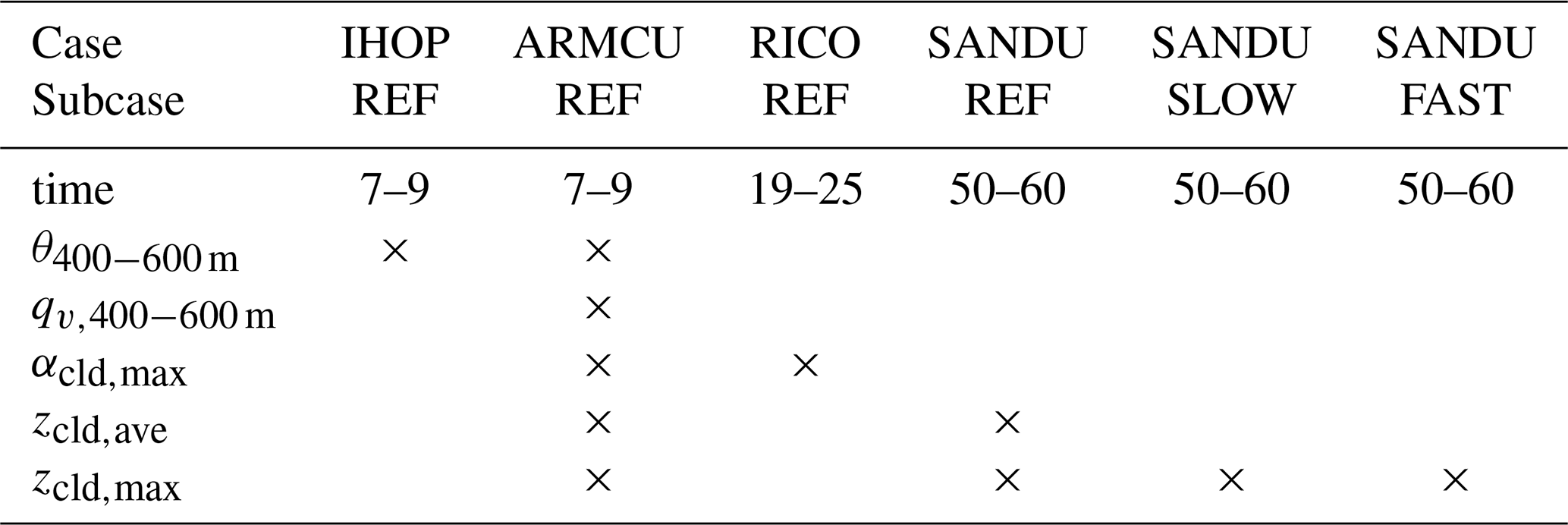
A long standing issue in parameterization development and improvement was the difficulty of retuning simultaneously the free parameters after a parameterization change, without which a physics improvement could be overled by a bad parameter tuning. This retuning is now made automatic thanks to the htexplo tool. The same tuning was applied here to the old model version and the new one with prognostic scheme. After a number of “waves”, we identify a number of configurations for both models, for which a series of metrics computed on SCM simulations of the IHOP, ARMCU, RICO and SANDU cases (Couvreux et al., 2021; Hourdin et al., 2021) match the metrics values computed on LES to less than a given tolerance to error σ. We use the same metrics as in Sect. 5.1 of Hourdin et al. (2021). These metrics are based on three model variables: potential temperature, humidity and cloud fraction. They are defined as temporal and spatial integrations over time and altitudes. For cloud fraction, three specific metrics are used: the first one is linked to the maximum cloud fraction on the vertical α_cld,max, the second one represents an average altitude of clouds z_cld,ave, and the last one corresponds to the altitude of the maximum cloud fraction z_cld,max, computed as an averaged altitude weighted by the fourth power of the cloud fraction. Table 1 details all the different metrics used in this tuning (the three cloud metrics, and those concerning potential temperature θ and humidity q_v).

Table 1 Metrics for the 1D/LES tuning. Time average is given in hours from the beginning of the simulation. Potential temperature is given in K, humidity in kg kg⁻¹ and height in m.

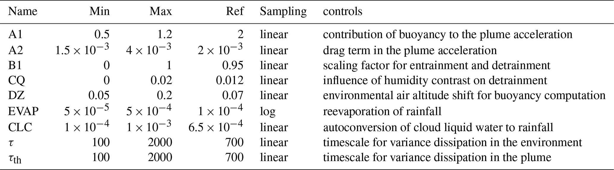
The free parameters are also kept the same as in Hourdin et al. (2021) except for the diagnostic model parameter of the diagnostic variance scheme BG1 and BG2 (Eqs. 15 and 14) which are replaced by parameters τ and τ_th in the prognostic scheme, allowed to vary between 100 and 2000 s. The other free parameters, common to both tuning exercises, are: (1) those involved in the modeling of the entrainment and detrainment rates of the thermal plume model (Eqs. 5 and 6): A1, B1, B2, CQ and DZ and (2) the CLC and EVAP parameters are involved in the precipitation and rain re-evaporation model, CLC being associated with the critical incloud water from which precipitation is activated and EVAP being a free parameter of the precipitation flux equation which controls the fraction of precipitation that re-evaporates at a given altitude. The formalism of these parameterizations was introduced by the work of Sundqvist (1978). Table 2 presents a summary of the different parameters to be tuned. More details on the parameterizations and free parameters can be found in Hourdin et al. (2021).

Table 2 Free parameters of the 1D/LES tuning.

4.2 Simulation scores according to the tuning tool

At each tuning wave, LMDZ SCM-simulations are computed within the range of authorized parameters by the previous wave (NROY: not-ruled out yet). For each of this simulations, a score is assigned per metric, this score being defined from the difference between the target value of the metric (the average value of the LES) and the value for the given simulation, as well as from the accepted tolerance. The closer the score is to 0, the closer the simulation metric is to the target value, a score equal to 1 indicates that the difference between the simulated metric and the target value corresponds exactly to the tolerance which we are willing to accept. The simulations can thus be classified according to the obtained scores, either on an average score criterion or on a maximum criterion. Here we use the maximum criterion to classify the ten most efficient simulations in order to prevent large errors on certain metrics from being compensated by very good results on others.

Figure 1 compares the results obtained on all the metrics between the diagnostic and prognostic models after 20 waves of tuning. From bottom to top, the figure displays the scores of the 10 best simulations across the 11 studied metrics. The second row shows the average score for each simulation, and the top row shows the maximum score of each simulation, corresponding to the worst score obtained among all metrics. As mentioned previously, the simulations are ranked according to the order of their maximum scores. In particular we see that the ten best simulations achieve almost identical maximum scores in both cases, close to 0.75 which means that the worst metric is at a distance of 0.75 σ from the target value. Note however that this score is obtained for a somewhat reduced tolerance to error σ in the case of the prognostic case for the metrics relative to the cloud height, z_cld,ave and z_cld,max. This lower values were adjusted since the new scheme was globally producing a better adjustment of the cloud height.

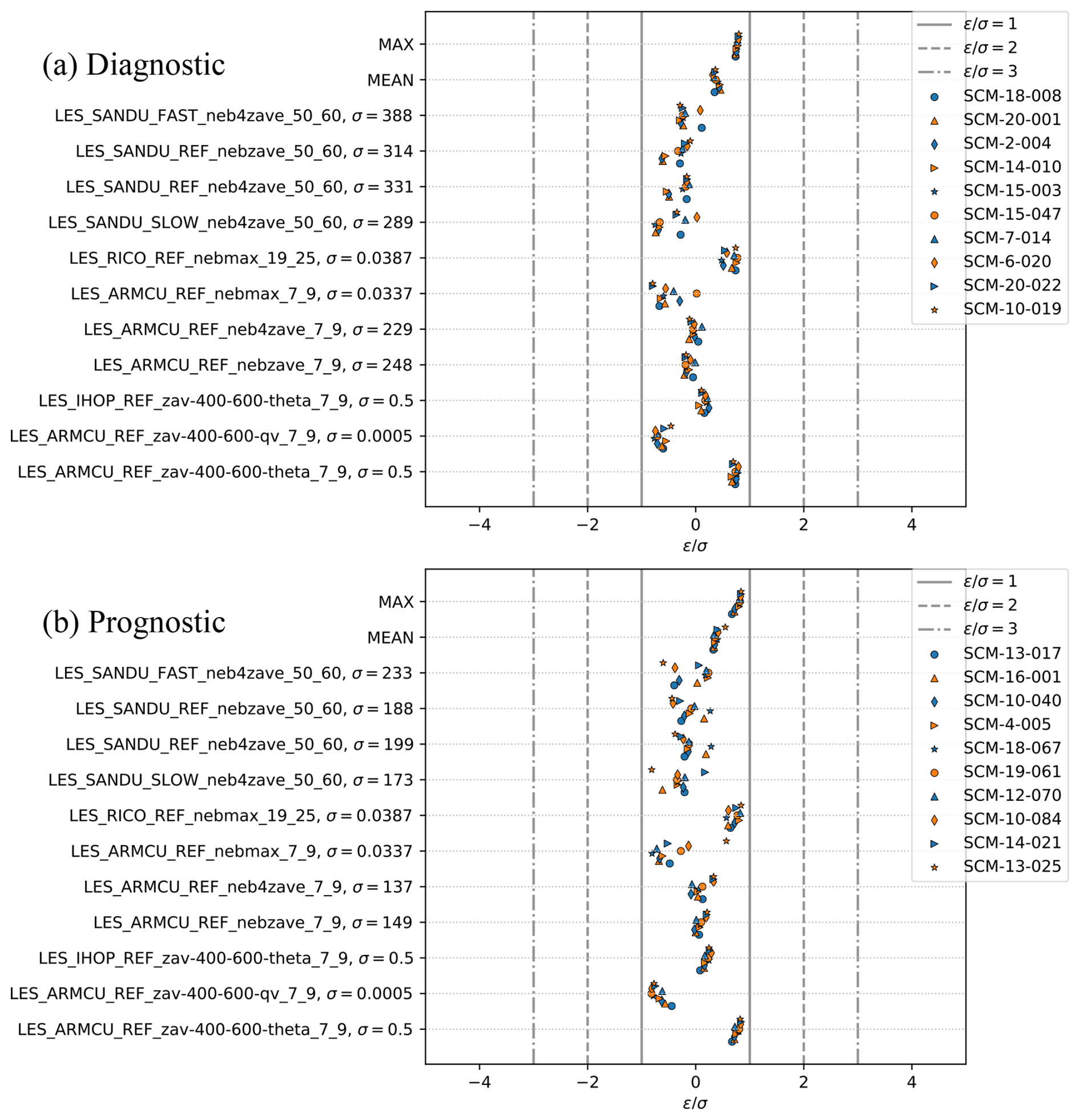
Figure 1 Metric scores ($\mathit{ϵ}/\mathit{\sigma }$) for the ten best simulations with (a) the previous diagnostic model and (b) the prognostic model. The SCM simulations are indexed by their wave number and by their number within that wave (out of 90 simulations per wave). The maximum and average scores of these ten best simulations are shown first, followed by their explicit scores for each metric. The 11 metrics are recalled on the left side with their acceptable margins of error σ.

It is important to underline that the tuning process does not aim to select an optimized configuration of the model but rather to highlight a range of parameters leading to acceptable results within the framework we have defined and the typical performance of the model in this range. In this context this tuning showed that the acceptable range of the relaxation time is 100 to 1300 s which is consistent with the previous qualitative considerations.

When using the TKE to define the relaxation time, the performance of the diagnostic scheme are comparable (results not shown) and the acceptable range of the mixing lengths shows up to be between 70 and 160 m.

4.3 Representation of the moments of the humidity distribution and cloud fraction

In this section, we focus on the variance, skewness, and cloud fraction profiles, which constitute the main diagnostics examined in this study. Most other physical quantities are only weakly affected by the change in the variance parameterization, as shown in Sect. 4.2. The results for the almost cloud-free IHOP case – used to control the potential temperature profile, which remains largely unchanged by the new parameterization – are not discussed here. Figure 2 presents the time evolution of the vertical cloud fraction profile simulated by the LES (left column) for the ARMCU, RICO, and SANDU cases, together with the differences between the LMDZ SCM and the LES for the diagnostic (middle) and prognostic models (right). Overall, the cloud fraction simulated by the two models remains very similar, with the prognostic formulation leading to a slight reduction in biases. Even if biased, the representation of the cloud fraction has been much improved in comparison with general model performances in simulating the ARM cumulus case 20 years ago (Lenderink et al., 2004), in particular regarding the cloud base and cloud top. Also, the RICO and SANDU cases involve precipitation processes and radiation, to which the cloud fraction simulated by LES is also quite sensitive (van Zanten et al., 2011; Sandu and Stevens, 2011).

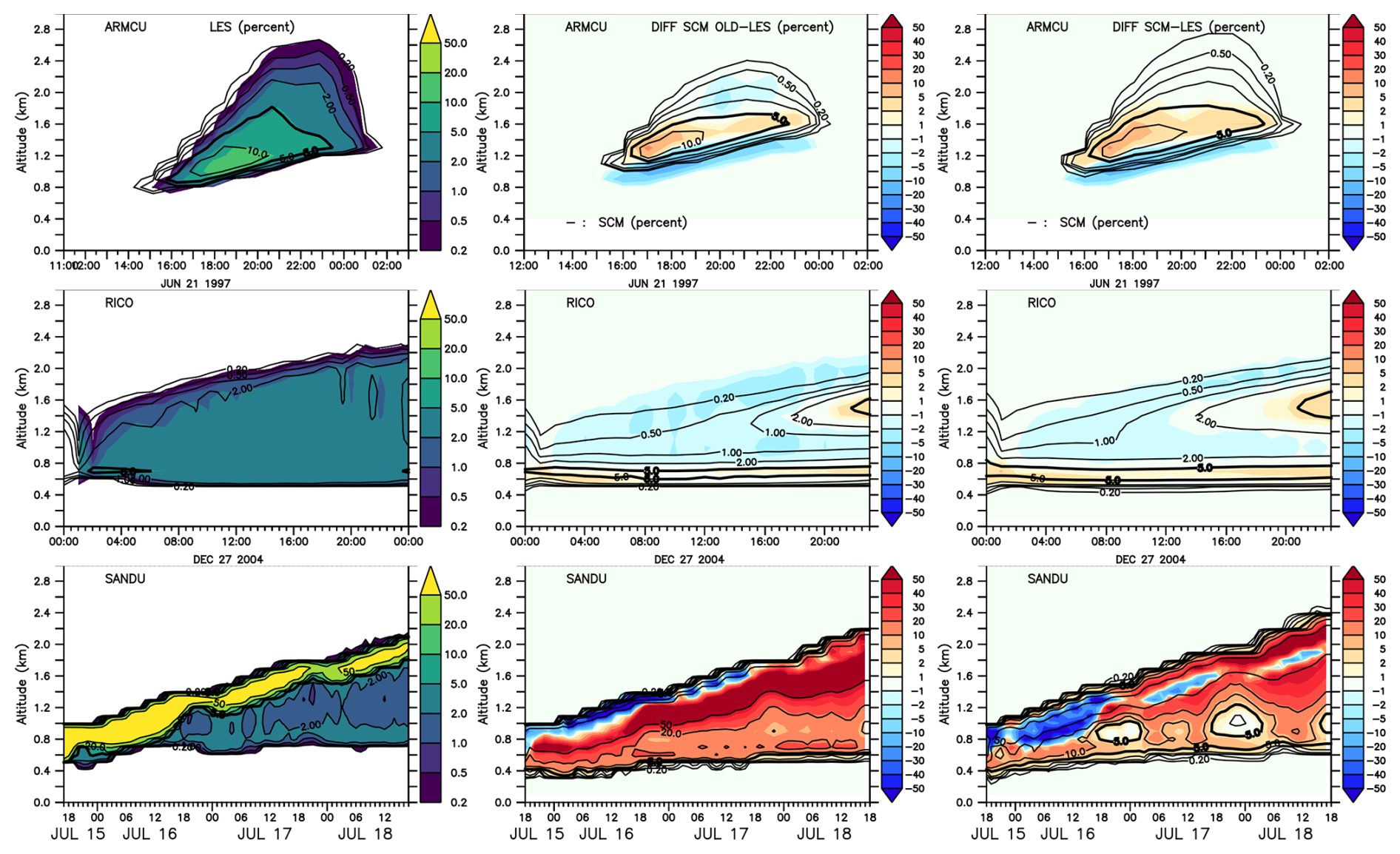
Figure 2 Total cloud fraction (%) in the ARMCU/REF (top), RICO/REF (middle) and SANDU/REF (bottom) cases. On the left the LES simulation. In the middle the difference in cloud fraction between the best tuning simulation with the old diagnostic model and the LES, black contours indicating the cloud fraction in the SCM simulation. On the right the difference in cloud fraction between the best tuning simulation with the prognostic model and the LES, black contours indicating the cloud fraction in the SCM simulation.

Figure 3 separates the total standard deviation into the standard deviation within thermals and within their environment, along with the corresponding difference in total specific humidity. Figure 4 shows the vertical profile of cloud fraction and the associated standard deviation of specific humidity for specific times of simulations, as well as the time evolution of the standard deviation averaged within the cloud layer. Figure 5 evaluates the representation of the third order moment and skewness.

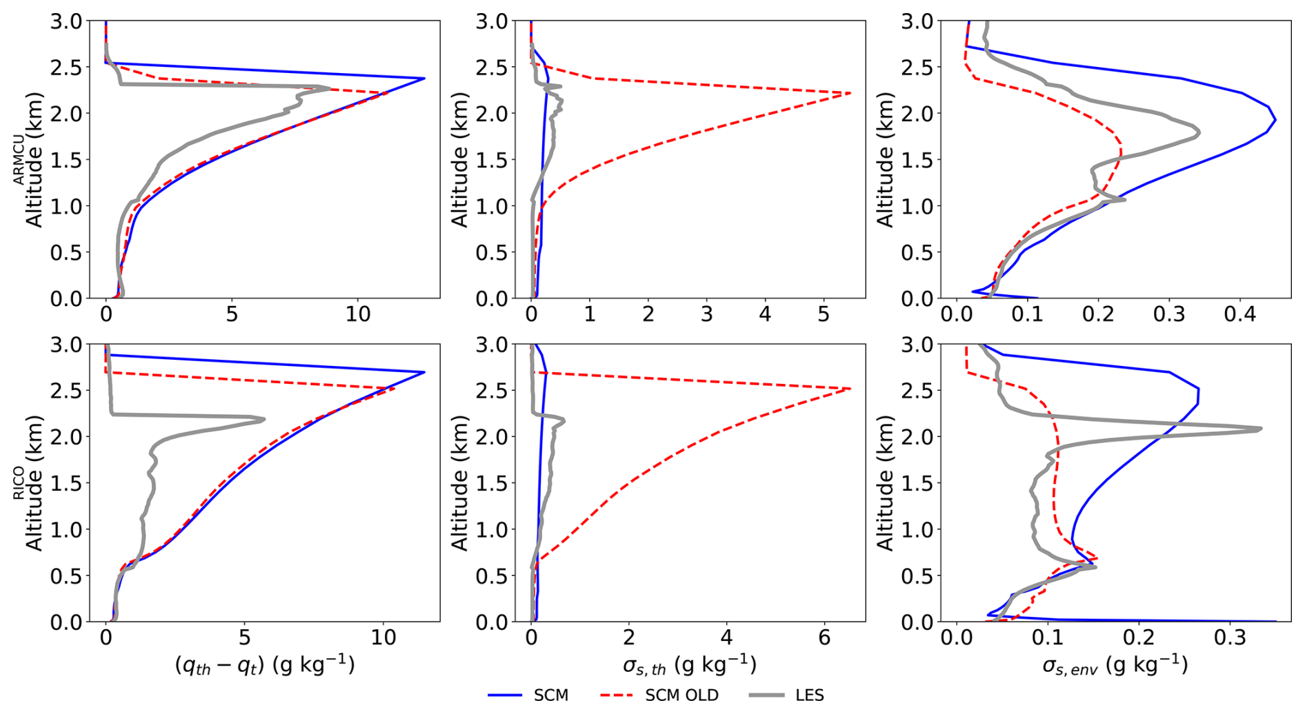
Figure 3 Difference in total specific humidity between thermals and the environment (left), standard deviation of the saturation deficit in the thermals (middle) and in the environment (right). Top ARMCU/REF at 19:00 LT, bottom RICO/REF at 20:00 LT. Blue: SCM with prognostic variance, dashed red: SCM with diagnostic variance, thick gray: LES.

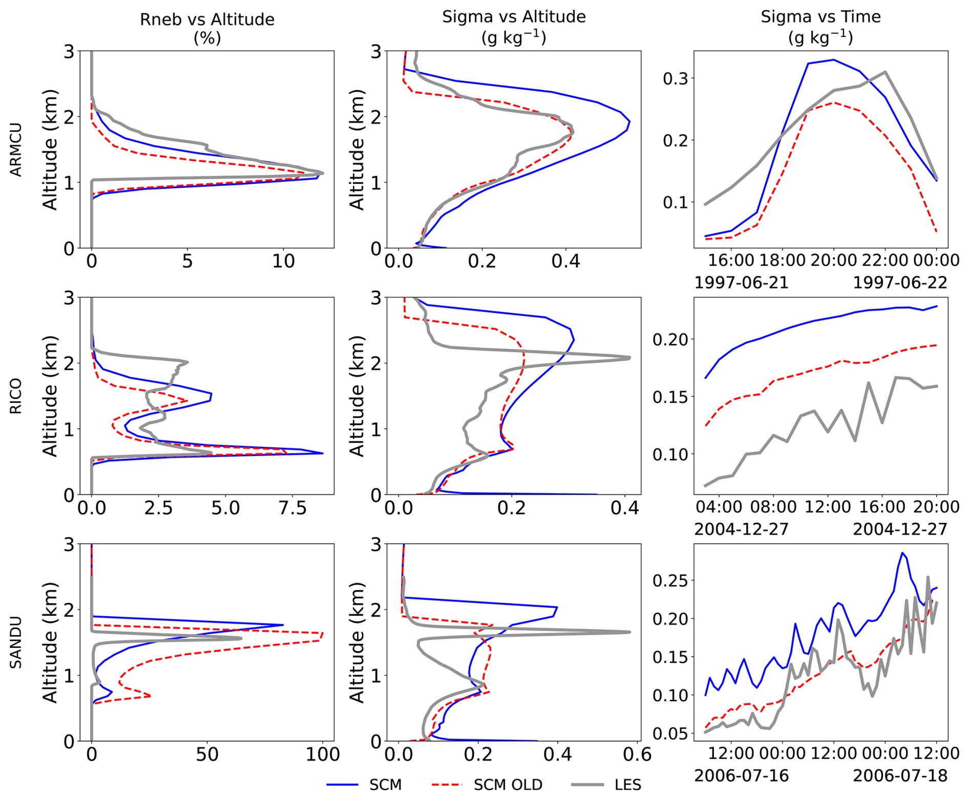
Figure 4 Cloud fraction and standard deviation of the saturation deficit, including the contribution of thermals, in the ARMCU/REF (top), RICO/REF (middle) and SANDU/REF (bottom) cases. Thick gray is the LES, blue is the LMDZ simulation with prognostic variance and dashed red with previous diagnostic model. On the left the cloud fraction profile at 19:00 LT for ARMCU, 20:00 LT for RICO and midnight on the last day for SANDU. In the middle the standard deviation of the saturation deficit profile at the same dates. On the right temporal evolutions of the averaged standard deviation between 500 and 2500 m for ARMCU and RICO and 400 and 2200 m for SANDU. These data were obtained with the best tuning simulations for each model.

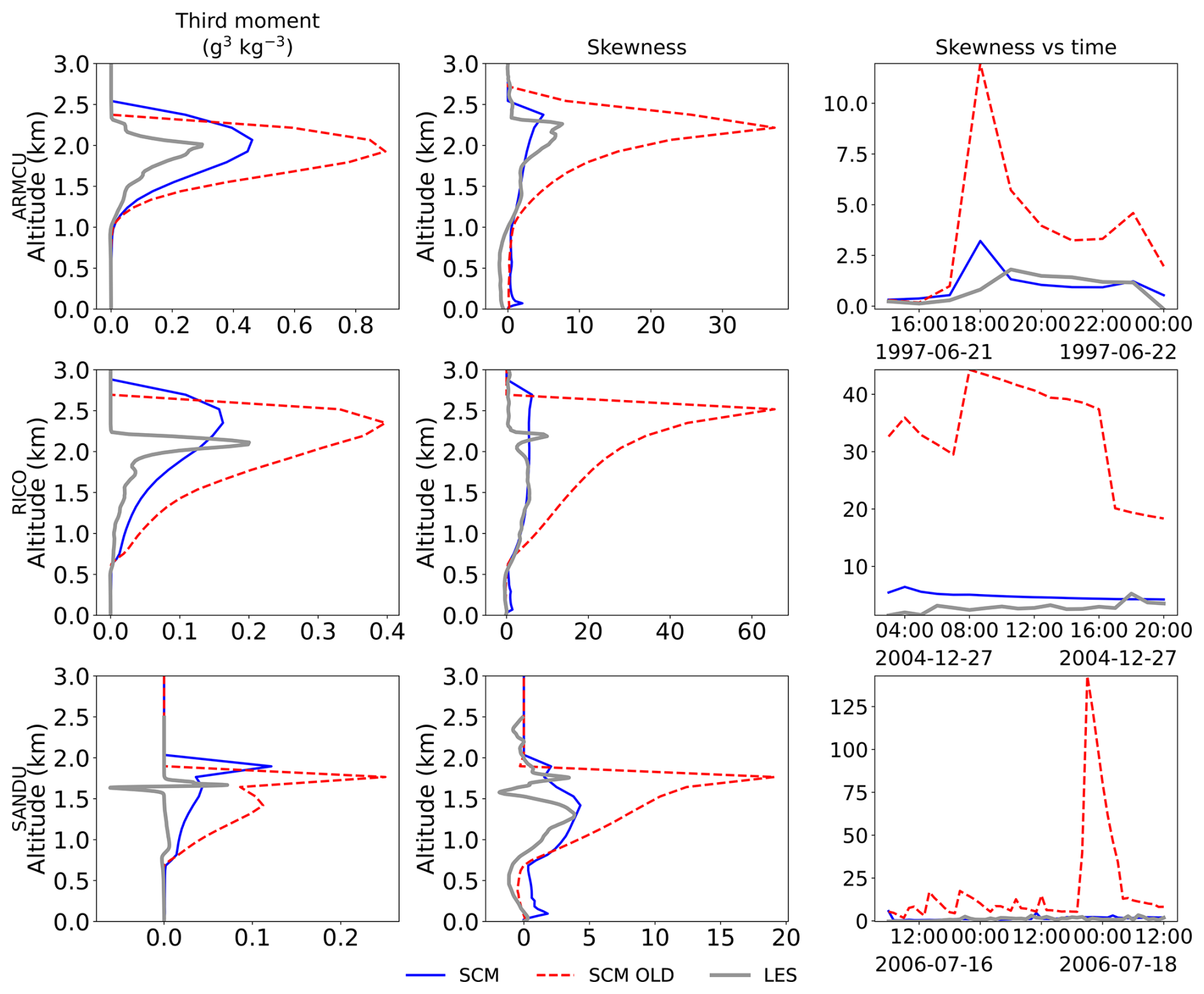
Figure 5 Centered third order moment (numerator of Eq. 11) of the saturation deficit distribution on the left, skewness of the saturation deficit distribution profile on the middle and its evolution in time averaged from 500 and 2500 m for ARMCU and RICO, and from 400 and 2200 m for SANDU on the right. Top ARMCU/REF, middle RICO/REF and bottom SANDU/REF. Left and middle profiles are represented at 19:00 LT for ARMCU, 20:00 LT for RICO and midnight on the last day for SANDU. Blue: SCM with prognostic variance, dashed red: SCM with diagnostic variance, thick gray: LES.

While the cloud fraction and the standard deviation of total specific humidity are quite close between the two model versions and the LES (Fig. 4), the prognostic model improves the representation of the standard deviation within thermals (Fig. 3). It can be seen that in the diagnostic model, the standard deviation is almost proportional to the specific humidity difference between the thermals and the environment and one order of magnitude too large. This strongly impacts the third-order moment (Fig. 5) through the first term of Eq. (11). This major flaw is largely corrected by the prognostic model, although the standard deviation is there slightly underestimated. The third-order moment, which reflects the asymmetry of the humidity distribution, is now in better agreement with the LES. This demonstrates that an improved representation of the higher moments of the distribution profiles can be obtained by simply exploiting the transport of q and q² within the thermals, with a tunable parameter that is easy to estimate using TKE. A possible flaw of the prognostic model is the lack of representation in the PDF of organized subsiding structures which tend to locally dry out the environment. Although subsidences are taken into account as sources of variance, they cannot negatively impact the third order moment because of the binary structure of our PDF with only thermal plume and environment. This is particularly visible in rare areas of negative skewness but it should not overshadow the quite accurate estimation of the third-order moments of the model.

Figure 6 further shows the contribution of the different terms of Eq. (18) in the variance transport. It shows the clear predominance of the first term of the variance transport equation, a term which represents the squared difference in humidity between thermals and environment. The two other terms, difference of variance and subsidence, appear to be an order of magnitude smaller so that they could be neglected if one wants to simplify the implementation of the explicit transport equation in the model. This result is specific to shallow convective cases, where the standard deviations of humidity, both in thermals and in the environment, are small compared to the mean values and their difference (see Fig. 3). In contrast, in a deep convective case, such as that studied in K05, the ratio r = $\frac{\mathit{\sigma }}{q_{\mathrm{t}}}$ is much higher, and one can therefore expect a significant impact from the variance difference term. K05 indeed shows that, in this case, the variance difference term is of the same order of magnitude as the squared humidity difference term. This point should not be overlooked when extending this study to deep convection cases. In that context, however, particular attention will also need to be paid to precipitating downdrafts, which can have a significant, and often negative, impact on the variance and skewness.

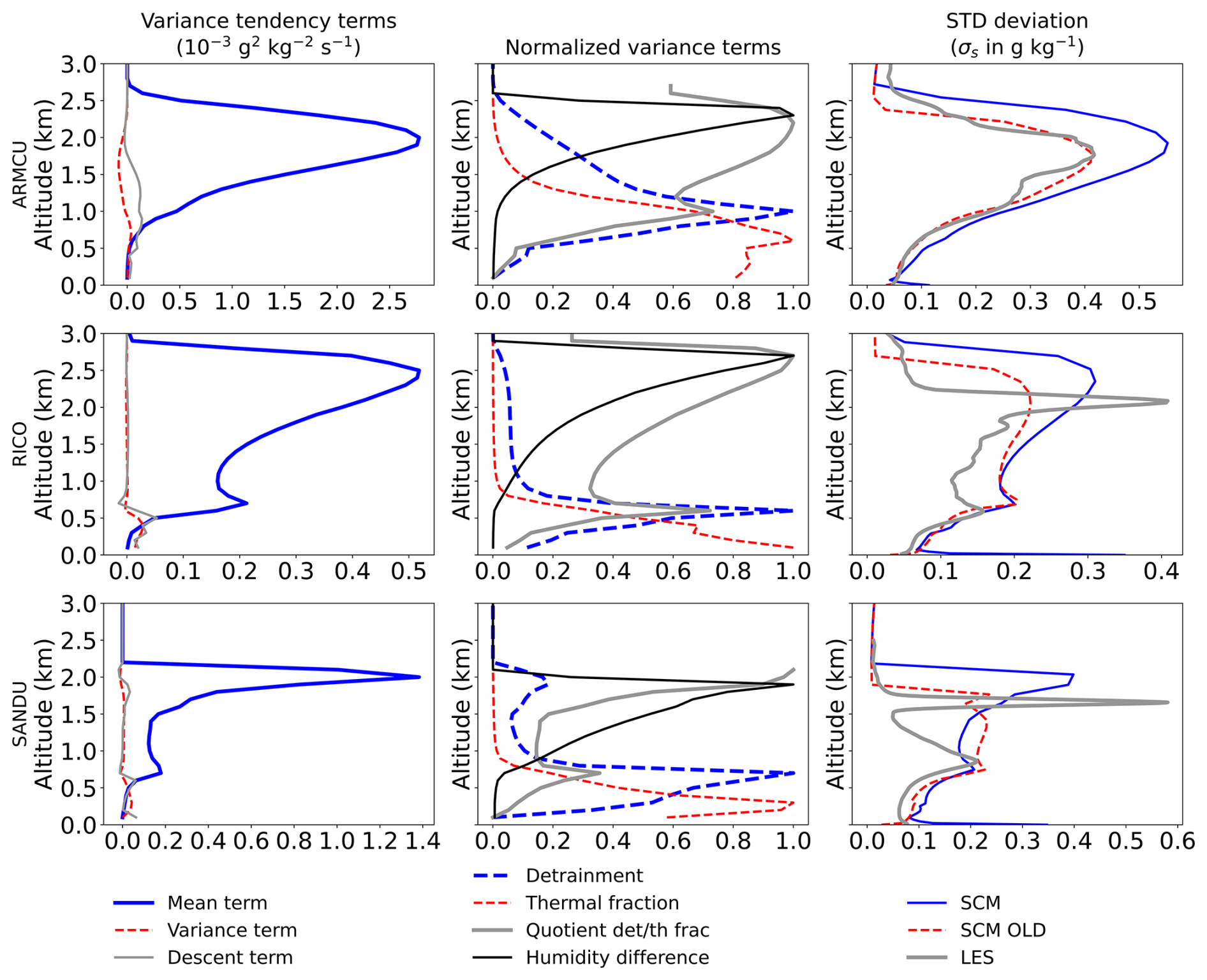
Figure 6 Various profiles in the ARMCU/REF (top) RICO/REF (middle) and SANDU/REF (bottom) cases. On the left: comparison between the 3 source terms of variance in Eq. (18), blue being $\frac{d}{\mathit{\rho }}(\stackrel{\mathrm{‾}}{q_{\mathrm{th}}}-\stackrel{\mathrm{‾}}{q}{)}^{\mathrm{2}}$ the squared mean difference term, dashed red the variance difference term $\frac{d}{\mathit{\rho }}(\stackrel{\mathrm{‾}}{q_{\mathrm{th}}^{\prime \mathrm{2}}}-\stackrel{\mathrm{‾}}{q^{\prime \mathrm{2}}})$ and thick gray the subsidence term $\frac{f}{\mathit{\rho }}\frac{\partial \stackrel{\mathrm{‾}}{q^{\prime \mathrm{2}}}}{\partial z}$. In the middle the normalized profiles of some physical quantities involved in the variance model: the detrainment rate d (thick dashed blue), the thermal fraction multiplicative term in the diagnostic model $\frac{{\mathit{\alpha }}^{{\mathit{\gamma }}_{\mathrm{1}}}}{\mathrm{1}-\mathit{\alpha }}$ (dashed red) and the square of the total humidity difference between thermal and environment $({\stackrel{\mathrm{‾}}{q}}_{\mathrm{th}}-{\stackrel{\mathrm{‾}}{q}}_{\mathrm{env}}{)}^{\mathrm{2}}$ (black). The quotient of the detrainement term by the termal fraction term is also represented (thick gray). On the right the total humidity variance profiles are remained: blue for the prognostic variance model, dashed red for the diagnostic one and thick gray for the LES. This profiles were computed at 19:00 LT for ARMCU, 20:00 LT for RICO and midnight on the last day for SANDU.

Accurately representing the vertical profile of cloud fraction during the stratocumulus-to-cumulus transition remains particularly challenging (SANDU case). Hourdin et al. (2019) showed that a carefully tuned modification of the detrainment parameterization represents an important first step toward simulating this transition. However, Fig. 2 shows that the cloud fraction still tends to remain saturated with the diagnostic model while it gradually fades in the LES. Moreover this cloud fraction is too thick at night in LMDZ especially from the second day of the simulation where it becomes significantly finer in the LES, leading to sometimes large differences in Fig. 2. Figures 2 and 4 show that both aspects are attenuated with the variance prognostic model, even though some notable differences still persist. Looking deeper at the variance profile, we can attribute this improvement to a better representation of the variance peak at the top of the clouds. Let's remind, indeed, that an increase in the variance of the statistical cloud scheme, in case of high cloud fraction, is likely to reduce the cloud fraction by increasing the fraction of air with lower humidity. This better representation of the variance peak can partly be attributed to the thermal plume detrainment peak in this area as we can see in Fig. 6 (in the middle bottom) even if this peak occurs a little too high. In fact, the detrainment is directly involved in the variance transport equation but was not taken into account in the diagnostic model which rather involves a term dependent on the thermal fraction (dashed red curve in the middle of Fig. 6). This term vanishes to zero while the detrainment reaches its peak which explains the difference in behavior between the two models. We can notice, however, that the difference in humidity between thermals and environment also plays a crucial role at these altitudes (in black in Fig. 6 in the middle) but in the diagnostic model this term is multiplied by a factor which tends quickly to zero while in the prognostic model the multiplicative factor, which depends on the detrainment, cancels out higher and can even reach a local maximum at the top of the clouds.

5 Conclusions

This study first confirms that the choice of a weighted bivariate Gaussian PDF, based on the fraction of thermals, provides a satisfactory framework for representing the asymmetric distribution of humidity at different atmospheric levels especially when associated with the prognostic variance model, which helps avoid inconsistent behaviors of the saturation deficit in the thermals and at the cloud tops through the thermal detrainment term.

It shows how the heuristic parameterization of the width of the two Gaussian proposed by Jam et al. (2013) can be replaced by a prognostic model of the variance of the total specific humidity whose physical content is based on a general transport equations.

In the context of shallow convection considered here, we make use of the thermal plume model in which the specific humidity is treated as a conservative variable. This property is used to transport its square and to derive the equation of evolution of the variance by assimilating the diffusive homogenization to a simple Newtonian relaxation of the humidity variance toward zero, both in the plume and in its environment, involving a time parameter which can be estimated from the TKE.

The new approach, coupling the thermal plume model, and a bi-Gaussian cloud scheme with width computed from the prognostic equation of q², was implemented in the LMDZ model and tested in SCM mode against LES results on cumulus and transition test cases.

Thanks to an automatic tuning of the model free parameters, we were able to obtain results consistent with those obtained previously with the diagnostic model of the Gaussian widths.

The new approach significantly improves the representation of the higher moments of the specific humidity distribution without degrading, or even improving slightly the representation of cloud fractions.

These improvements are closely related to the consideration of detrainment, which plays a key role in the prognostic equations of the variance. Certain inaccuracies of the diagnostic model could therefore be corrected, in particular in the thermal plumes and at the top of the clouds where detrainment is significant.

Note however that the present study is restricted to cases of shallow convection and that the variance model only accounts so far for source terms coming from thermal plumes and sink coming from small scale turbulence.

Negative asymmetries due to downdrafts cannot be accounted so far within the framework with the bi-Gaussian scheme.

Furthermore, subsiding shells, whose convective transport contribution can reach from 5 % to 10 % (Glenn and Krueger, 2013; Savre, 2021; Brient et al., 2023), are not explicitly represented in our mass-flux model. However, as previously said, the detrainment parameterization includes certain aspects that indirectly account for their influence. The parameterization of sub-cloud layer downdrafts, also referred to as dry tongues (Couvreux et al., 2007), is currently under development and could further contribute to the variance budget.

This study focuses on liquid boundary-layer clouds. In the presence of ice, beyond thermodynamic effects associated with latent heat release (which enhances thermal updrafts), additional microphysical processes (e.g., condensation nuclei, supersaturation) should be considered and are indeed an active area of research within LMDZ.

As a natural extension of this study, we are working on integrating the formalism of the Emanuel's scheme for deep convection into the variance model and further source terms associated with convective transport and evaporation of precipitation, with a particular focus on representing the impact of precipitating downdrafts from the Emanuel scheme on specific humidity variance. In contrast to shallow convection, these downdrafts are expected to have a significant effect on variance. Two competing processes may be involved: a drying effect associated with the descent of dry air, and a moistening effect linked to rain re-evaporation.

The final objective would be to transport the large-scale variance as a state variable in the dynamics of the GCM with the same approach proposed in the present study. This work is therefore an important step to incorporate into a GCM a unified global model of the upper moments of the atmospheric specific humidity relying on the fundamental physical equations and with a minimum of free parameters. It has helped to improve our understanding of the role of thermal updrafts in the variability of specific humidity, particularly through the detrainment process.

Appendix A: Calculation of second- and third-order moments of saturation deficit

A1 Second order moment of saturation deficit

The second order moment of saturation deficit writes by simply separating the spatial average into a thermal part and an environmental part:

$$\begin{array}{}\text{(A1)}& {\mathit{\sigma }}^{\mathrm{2}}=\stackrel{\mathrm{‾}}{s^{\prime \mathrm{2}}}=\stackrel{\mathrm{‾}}{{\left(s-\stackrel{\mathrm{‾}}{s}\right)}^{\mathrm{2}}}=\mathit{\alpha }\stackrel{\mathrm{‾}}{s_{\mathrm{th}}^{\prime \mathrm{2}}}+\left(\mathrm{1}-\mathit{\alpha }\right)\stackrel{\mathrm{‾}}{s_{\mathrm{env}}^{\prime \mathrm{2}}}.\end{array}$$

Let us calculate the two terms separately:

$$\begin{array}{}\text{(A2)}& \begin{array}{rl}\stackrel{\mathrm{‾}}{s_{\mathrm{th}}^{\prime \mathrm{2}}}& =\stackrel{\mathrm{‾}}{{\left(s_{\mathrm{th}}-\stackrel{\mathrm{‾}}{s}\right)}^{\mathrm{2}}}=\stackrel{\mathrm{‾}}{{\left(s_{\mathrm{th}}-\stackrel{\mathrm{‾}}{s_{\mathrm{th}}}+\stackrel{\mathrm{‾}}{s_{\mathrm{th}}}-\stackrel{\mathrm{‾}}{s}\right)}^{\mathrm{2}}}\\ & =\stackrel{\mathrm{‾}}{{\left(s_{\mathrm{th}}-\stackrel{\mathrm{‾}}{s_{\mathrm{th}}}\right)}^{\mathrm{2}}}+{\left(\stackrel{\mathrm{‾}}{s_{\mathrm{th}}}-\stackrel{\mathrm{‾}}{s}\right)}^{\mathrm{2}}+\mathrm{2}\stackrel{\mathrm{‾}}{\left(s_{\mathrm{th}}-\stackrel{\mathrm{‾}}{s_{\mathrm{th}}}\right)}\left(\stackrel{\mathrm{‾}}{s_{\mathrm{th}}}-\stackrel{\mathrm{‾}}{s}\right)\end{array}\end{array}$$

The last term is zero, the first one is the variance ${\mathit{\sigma }}_{\mathrm{th}}^{\mathrm{2}}$ of the saturation deficit in the thermal part, and the middle one can be rearranged as follow noting that $\stackrel{\mathrm{‾}}{s}=\mathit{\alpha }\stackrel{\mathrm{‾}}{s_{\mathrm{th}}}+(\mathrm{1}-\mathit{\alpha })\stackrel{\mathrm{‾}}{s_{\mathrm{env}}}$:

$$\begin{array}{}\text{(A3)}& {\left(\stackrel{\mathrm{‾}}{s_{\mathrm{th}}}-\stackrel{\mathrm{‾}}{s}\right)}^{\mathrm{2}}={\left(\mathrm{1}-\mathit{\alpha }\right)}^{\mathrm{2}}{\left(\stackrel{\mathrm{‾}}{s_{\mathrm{th}}}-\stackrel{\mathrm{‾}}{s_{\mathrm{env}}}\right)}^{\mathrm{2}}\end{array}$$

Finally it leads to:

$$\begin{array}{}\text{(A4)}& \stackrel{\mathrm{‾}}{s_{\mathrm{th}}^{\prime \mathrm{2}}}={\mathit{\sigma }}_{\mathrm{th}}^{\mathrm{2}}+{\left(\mathrm{1}-\mathit{\alpha }\right)}^{\mathrm{2}}{\left(\stackrel{\mathrm{‾}}{s_{\mathrm{th}}}-\stackrel{\mathrm{‾}}{s_{\mathrm{env}}}\right)}^{\mathrm{2}}\end{array}$$

In the same way we calculate:

$$\begin{array}{}\text{(A5)}& \begin{array}{rl}\stackrel{\mathrm{‾}}{s_{\mathrm{env}}^{\prime \mathrm{2}}}& =\stackrel{\mathrm{‾}}{{\left(s_{\mathrm{env}}-\stackrel{\mathrm{‾}}{s}\right)}^{\mathrm{2}}}=\stackrel{\mathrm{‾}}{{\left(s_{\mathrm{env}}-\stackrel{\mathrm{‾}}{s_{\mathrm{env}}}+\stackrel{\mathrm{‾}}{s_{\mathrm{env}}}-\stackrel{\mathrm{‾}}{s}\right)}^{\mathrm{2}}}\\ & =\stackrel{\mathrm{‾}}{{\left(s_{\mathrm{env}}-\stackrel{\mathrm{‾}}{s_{\mathrm{env}}}\right)}^{\mathrm{2}}}+{\left(\stackrel{\mathrm{‾}}{s_{\mathrm{env}}}-\stackrel{\mathrm{‾}}{s}\right)}^{\mathrm{2}}\\ & +\mathrm{2}\stackrel{\mathrm{‾}}{\left(s_{\mathrm{env}}-\stackrel{\mathrm{‾}}{s_{\mathrm{env}}}\right)}\left(\stackrel{\mathrm{‾}}{s_{\mathrm{env}}}-\stackrel{\mathrm{‾}}{s}\right)\end{array}\end{array}$$

which becomes:

$$\begin{array}{}\text{(A6)}& \stackrel{\mathrm{‾}}{s_{\mathrm{env}}^{\prime \mathrm{2}}}={\mathit{\sigma }}_{\mathrm{env}}^{\mathrm{2}}+{\mathit{\alpha }}^{\mathrm{2}}{\left(\stackrel{\mathrm{‾}}{s_{\mathrm{th}}}-\stackrel{\mathrm{‾}}{s_{\mathrm{env}}}\right)}^{\mathrm{2}}\end{array}$$

By introducing Eqs. (A4) and (A6) into Eq. (A1), we obtain as announced:

$$\begin{array}{}\text{(A7)}& V={\mathit{\sigma }}^{\mathrm{2}}=\stackrel{\mathrm{‾}}{s^{\prime \mathrm{2}}}=\mathit{\alpha }{\mathit{\sigma }}_{\mathrm{th}}^{\mathrm{2}}+(\mathrm{1}-\mathit{\alpha }){\mathit{\sigma }}_{\mathrm{env}}^{\mathrm{2}}+\mathit{\alpha }(\mathrm{1}-\mathit{\alpha }){\left(\stackrel{\mathrm{‾}}{s_{\mathrm{th}}}-\stackrel{\mathrm{‾}}{s_{\mathrm{env}}}\right)}^{\mathrm{2}}\end{array}$$

A2 Third order moment of saturation deficit

In the same way, we derive the expression for the third-order moment:

$$\begin{array}{}\text{(A8)}& M_{\mathrm{3}}=\stackrel{\mathrm{‾}}{s^{\prime \mathrm{3}}}=\stackrel{\mathrm{‾}}{{\left(s-\stackrel{\mathrm{‾}}{s}\right)}^{\mathrm{3}}}=\mathit{\alpha }\stackrel{\mathrm{‾}}{s_{\mathrm{th}}^{\prime \mathrm{3}}}+(\mathrm{1}-\mathit{\alpha })\stackrel{\mathrm{‾}}{s_{\mathrm{env}}^{\prime \mathrm{3}}}\end{array}$$

Which splits into

$$\begin{array}{}\text{(A9)}& \begin{array}{rl}\stackrel{\mathrm{‾}}{s_{\mathrm{th}}^{\prime \mathrm{3}}}& =\stackrel{\mathrm{‾}}{{\left(s_{\mathrm{th}}-\stackrel{\mathrm{‾}}{s}\right)}^{\mathrm{3}}}=\stackrel{\mathrm{‾}}{(s_{\mathrm{th}}-\stackrel{\mathrm{‾}}{s_{\mathrm{th}}}+\stackrel{\mathrm{‾}}{s_{\mathrm{th}}}-\stackrel{\mathrm{‾}}{s}{)}^{\mathrm{3}}}\\ & =\stackrel{\mathrm{‾}}{{\left(s_{\mathrm{th}}-\stackrel{\mathrm{‾}}{s_{\mathrm{th}}}\right)}^{\mathrm{3}}}+{\left(\stackrel{\mathrm{‾}}{s_{\mathrm{th}}}-\stackrel{\mathrm{‾}}{s}\right)}^{\mathrm{3}}+\mathrm{3}\stackrel{\mathrm{‾}}{{\left(s_{\mathrm{th}}-\stackrel{\mathrm{‾}}{s_{\mathrm{th}}}\right)}^{\mathrm{2}}}\left(\stackrel{\mathrm{‾}}{s_{\mathrm{th}}}-\stackrel{\mathrm{‾}}{s}\right)\end{array}\end{array}$$

by noting that $\mathrm{3}\stackrel{\mathrm{‾}}{\left(s_{\mathrm{th}}-\stackrel{\mathrm{‾}}{s_{\mathrm{th}}}\right)}{\left(\stackrel{\mathrm{‾}}{s_{\mathrm{th}}}-\stackrel{\mathrm{‾}}{s}\right)}^{\mathrm{2}}$ = 0. In our framework, the distribution of the saturation deficit is Gaussian in the thermal part. Therefore, the first term of Eq. (A9), which represents the third-order moment in the thermal part, is zero. Thus, using Eq. (A3), it remains:

$$\begin{array}{}\text{(A10)}& \stackrel{\mathrm{‾}}{s_{\mathrm{th}}^{\prime \mathrm{3}}}=(\mathrm{1}-\mathit{\alpha }{)}^{\mathrm{3}}{\left(\stackrel{\mathrm{‾}}{s_{\mathrm{th}}}-\stackrel{\mathrm{‾}}{s_{\mathrm{env}}}\right)}^{\mathrm{3}}+\mathrm{3}{\mathit{\sigma }}_{\mathrm{th}}^{\mathrm{2}}(\mathrm{1}-\mathit{\alpha })\left(\stackrel{\mathrm{‾}}{s_{\mathrm{th}}}-\stackrel{\mathrm{‾}}{s_{\mathrm{env}}}\right)\end{array}$$

By applying the same reasoning in the environmental part:

$$\begin{array}{}\text{(A11)}& \begin{array}{rl}\stackrel{\mathrm{‾}}{s_{\mathrm{env}}^{\prime \mathrm{3}}}& =\stackrel{\mathrm{‾}}{{\left(s_{\mathrm{env}}-\stackrel{\mathrm{‾}}{s}\right)}^{\mathrm{3}}}=\stackrel{\mathrm{‾}}{{\left(s_{\mathrm{env}}-\stackrel{\mathrm{‾}}{s_{\mathrm{env}}}+\stackrel{\mathrm{‾}}{s_{\mathrm{env}}}-\stackrel{\mathrm{‾}}{s}\right)}^{\mathrm{3}}}\\ & =\stackrel{\mathrm{‾}}{{\left(s_{\mathrm{env}}-\stackrel{\mathrm{‾}}{s_{\mathrm{env}}}\right)}^{\mathrm{3}}}+{\left(\stackrel{\mathrm{‾}}{s_{\mathrm{env}}}-\stackrel{\mathrm{‾}}{s}\right)}^{\mathrm{3}}\\ & +\mathrm{3}\stackrel{\mathrm{‾}}{{\left(s_{\mathrm{env}}-\stackrel{\mathrm{‾}}{s_{\mathrm{env}}}\right)}^{\mathrm{2}}}\left(\stackrel{\mathrm{‾}}{s_{\mathrm{env}}}-\stackrel{\mathrm{‾}}{s}\right)\end{array}\end{array}$$

which leads to:

$$\begin{array}{}\text{(A12)}& \stackrel{\mathrm{‾}}{s_{\mathrm{env}}^{\prime \mathrm{3}}}={\mathit{\alpha }}^{\mathrm{3}}{\left(\stackrel{\mathrm{‾}}{s_{\mathrm{env}}}-\stackrel{\mathrm{‾}}{s_{\mathrm{th}}}\right)}^{\mathrm{3}}+\mathrm{3}{\mathit{\sigma }}_{\mathrm{env}}^{\mathrm{2}}\mathit{\alpha }\left(\stackrel{\mathrm{‾}}{s_{\mathrm{env}}}-\stackrel{\mathrm{‾}}{s_{\mathrm{th}}}\right)\end{array}$$

And after some simple algebra we obtain the third-order moment by injecting Eqs. (A10) and (A12) into Eq. (A8):

$$\begin{array}{}\text{(A13)}& \begin{array}{rl}{M}_{\mathrm{3}}& =\mathrm{3}\mathit{\alpha }(\mathrm{1}-\mathit{\alpha })\left(\stackrel{\mathrm{‾}}{s_{\mathrm{th}}}-\stackrel{\mathrm{‾}}{s_{\mathrm{env}}}\right)\left({\mathit{\sigma }}_{\mathrm{th}}^{\mathrm{2}}-{\mathit{\sigma }}_{\mathrm{env}}^{\mathrm{2}}\right)\\ & +\mathit{\alpha }\left(\mathrm{1}-\mathrm{3}\mathit{\alpha }+\mathrm{2}{\mathit{\alpha }}^{\mathrm{2}}\right){\left(\stackrel{\mathrm{‾}}{s_{\mathrm{th}}}-\stackrel{\mathrm{‾}}{s_{\mathrm{env}}}\right)}^{\mathrm{3}}\end{array}\end{array}$$

The skewness is then obtained by dividing by $V^{\frac{\mathrm{3}}{\mathrm{2}}}$ as in the main text (Eq. 11).