Satellite observations reveal heterogeneous atmospheric composition responses to rapid emission changes

We developed a unified machine learning framework to retrieve daily, 1 km resolution, gap-free concentrations of six major atmospheric pollutants across China, providing a consistent basis for quantifying atmospheric composition responses to rapid emission perturbations. Our results reveal pronounced spatiotemporal variability across pollutant species, with recovery times ranging from two to eight weeks following abrupt emission reductions. Most air pollutants, such as particulate matter (PM) and NO₂, exhibited rapid declines and subsequent rebounds, consistent with changes in anthropogenic emissions, whereas O₃ showed the opposite response, reflecting nonlinear photochemical processes under reduced NO_x conditions. In contrast, SO₂ and CO displayed more sustained decreases, indicating longer-term structural changes in combustion-related sources. By integrating explainable artificial intelligence with atmospheric predictors, we disentangle meteorological and emission-driven contributions to the variability of secondary pollutants across spatial scales. In Wuhan, reduced anthropogenic emissions contributed to a 22 % decrease in PM_2.5 during the emission-reduction period, whereas enhanced atmospheric oxidation associated with meteorological variability led to a 40 % increase in O₃. During the subsequent recovery phase, meteorological factors dominated interannual variability, driving a 16 % rebound in PM_2.5 but a 5 % decline in O₃. These findings elucidate the chemical and physical mechanisms governing atmospheric composition under rapid perturbations in emissions and underscore the nonlinear coupling among primary emissions, secondary formation, and meteorological processes.

1 Introduction

Rapid and large-scale changes in anthropogenic emissions provide natural experiments for understanding the chemical and physical processes governing atmospheric composition. The abrupt reduction in human activities in China during early 2020 led to substantial short-term emission perturbations (Venter et al., 2020; Cooper et al., 2022; Wei et al., 2023b), offering a unique opportunity to investigate the response of multiple atmospheric pollutants to altered precursor emissions. As restrictions eased and human activities resumed, air quality and pollutant levels adjusted accordingly. These perturbations occurred against the backdrop of long-term emission control policies, such as the Blue Sky Protection Campaign (2018–2020), which further shaped atmospheric dynamics. However, the heterogeneous responses of different pollutant species and the mechanisms governing their evolution during subsequent emission recovery phases remain incompletely understood.

A growing body of research has examined pollutant changes during the emission-reduction period in China. For example, Wang and Zhang (2020) observed significant decreases in ground-based measurements of six major ambient air pollutants at the provincial level under strict activity restrictions, with 65 % of provinces showing normalized PM_2.5 and PM₁₀ concentrations below 80 % and 70 %, respectively, relative to historical levels. Cooper et al. (2022) found that surface NO₂ concentrations derived from TROPOMI data decreased by more than 10 ppbv in February in China, with declines persisting in eastern urban areas through April. These reductions were equivalent to more than three years of typical declines, and regions with the largest NO₂ decreases also showed greater local reductions in PM_2.5 levels. In contrast, Wei et al. (2022a) reported that surface O₃ concentrations, derived from satellite data using machine learning, increased substantially across eastern China during the lockdown, with relative changes exceeding 40 % in epidemic-hit areas, such as Hubei province and surrounding regions. Geng et al. (2024) found that emission reductions from industrial and socioeconomic activity led to a 14 % decrease in PM_2.5 exposure levels from January to April, simulated by the WRF/CMAQ model.

While short-term lockdowns initially had a significant impact on atmospheric pollutant levels and may have lasting effects, the subsequent rebound in anthropogenic emissions as restrictions eased could influence air pollutant levels in various ways in the following years. However, the evolution of atmospheric composition during these emission recovery phases has received comparatively less attention. Wang and Yang (2021) reported a varying-degree rebound in ground-measured air pollutants during April–September 2020 in nine Chinese cities, particularly for PM₁₀ and NO₂, which increased by 44 % and 87 % in September, respectively. They also observed a notably slower decline compared to the same period from 2017 to 2019, with concentrations occasionally exceeding the multi-year average. Guo et al. (2021) found that mean pollution levels and concentrations of six individual pollutants during May–October 2021 were 15 % and 8 %–38 % lower, respectively, than those of the same period in 2020 in the Beijing-Tianjin-Tangshan region, based on data from the China Air Quality Online Monitoring and Analysis Platform. Bhatti et al. (2022) observed increased air pollution during January–May 2021 in Jiangsu province, with PM₁₀ and NO₂ rising by 23 % and 16 %, respectively, resulting in a 3 % increase in the air quality index, according to the weather post report. Feng et al. (2022) reported that PM_2.5 concentrations increased by 22.3 µg m⁻³ in former lockdown cities during April–October 2020 compared to January–February 2020, while national levels remained lower than pre-lockdown 2019 values by 8.8–11.2 µg m⁻³, based on a weather-standardized pollutant dataset.

However, previous studies have largely focused on short-term air quality changes immediately following lockdowns, typically in specific regions and over limited periods, such as the early months of activity resumption. Most studies have also emphasized individual pollutants, such as PM_2.5 or NO₂, which reflect only the most severe pollutant at a given time. Furthermore, many analyses are based on heterogeneous datasets, particularly from ground-based measurements with limited spatial coverage due to the uneven distribution of monitoring stations in China. These limitations constrain the generalizability of findings and leave a critical gap in understanding nationwide air pollution conditions trends, especially in urban areas, where exposure and health risks are more pronounced. To date, no comprehensive assessment has fully captured the collective behavior of multiple air pollutants, particularly at fine spatial scales, where interactions among pollutants are more complex.

How has atmospheric composition evolved before, during, and after periods of rapid emission changes? What shifts have occurred in individual and composite pollutants, and what are the key drivers behind these changes? These questions can be addressed using advanced artificial intelligence (AI) models that leverage large-scale datasets spanning ground-based observations and satellite retrievals. In this study, we developed a state-of-the-art deep learning (DL) model to, for the first time, uniformly estimate six conventional outdoor air pollutants – fine particulate matter (PM_2.5), coarse particulate matter (PM₁₀), surface ozone (O₃), nitrogen dioxide (NO₂), sulfur dioxide (SO₂), and carbon monoxide (CO), primarily from satellite aerosol and trace gas retrievals at unprecedented spatial (1 km²) and temporal (daily) resolutions with complete coverage. Using this dataset, we investigate the spatiotemporal evolution of atmospheric composition across emission reduction and recovery phases and quantify the relative contributions of anthropogenic emissions and meteorological processes through explainable artificial intelligence. By examining coupled responses of primary and secondary pollutants across spatial scales, this study provides process-level insights into how rapid emission perturbations modulate atmospheric chemistry and composition.

2 Materials and Methods

2.1 Air pollutant modeling and validation

Air quality data were obtained from the ChinaHighAirPollutants (CHAP) database, developed by our team and extensively applied in environmental health studies. The CHAP database integrates ground observations, satellite retrievals, and chemical transport model simulations, addressing gaps in satellite data while capturing nonlinear relationships between satellite column retrievals and surface pollutant concentrations through advanced spatiotemporal artificial intelligence (AI) models. This integration yields a long-term, gap-free dataset with complete spatial coverage and high spatiotemporal resolution. In this study, six conventional air pollutants from 2019 to 2022 were analyzed, including two particulate species (PM_2.5 and PM₁₀) and four gaseous pollutants (i.e., O₃, NO₂, SO₂, and CO), all uniformly resolved at 1 km spatial resolution on a daily basis.

These AQ products are derived from the latest version, featuring substantial enhancements to key input variables within a unified AI framework – the four-dimensional spatiotemporal deep forest (4D-STDF) model – which aims to minimize inconsistencies across datasets and to ensure higher accuracy and reliability. A key improvement over the original deep forest model is the incorporation of spatiotemporal information. Spatial variability is represented using three spherical coordinate features derived from longitude (Lon) and latitude (Lat), i.e., $P_{\mathrm{s}}\sim [S_{\mathrm{1}},S_{\mathrm{2}},S_{\mathrm{3}}]=[\sin \left(\mathrm{2}\mathit{\pi }\frac{\text{Lon}}{\mathrm{360}}\right)$, $\cos \left(\mathrm{2}\mathit{\pi }\frac{\text{Lon}}{\mathrm{360}}\right)\sin \left(\mathrm{2}\mathit{\pi }\frac{\text{Lat}}{\mathrm{180}}\right)$, $\cos \left(\mathrm{2}\mathit{\pi }\frac{\text{Lon}}{\mathrm{360}}\right)\cos \left(\mathrm{2}\mathit{\pi }\frac{\text{Lat}}{\mathrm{180}}\right)$], which capture spatial autocorrelation patterns. Temporal variability is represented using three helix-shaped trigonometric features based on the normalized day of the year ($\frac{\text{DOY}}{N}$), i.e., $P_{\mathrm{t}}\sim [T_{\mathrm{1}},T_{\mathrm{2}},T_{\mathrm{3}}]=[\frac{\text{DOY}}{N}$, $\cos \left(\mathrm{2}\mathit{\pi }\frac{\text{DOY}}{N}\right)$, $\sin \left(\mathrm{2}\mathit{\pi }\frac{\text{DOY}}{N}\right)$], which capture both linear temporal progression and periodic (seasonal) variations. Together, these features enable the model to better represent daily variations and seasonal cycles in air pollution.

Specifically, PM_2.5 and PM₁₀ were estimated using MODIS MAIAC 1 km AOD products as the primary predictors (Wei et al., 2021), whereas surface concentrations of O₃ (Yang et al., 2025), NO₂ (Wei et al., 2022b), SO₂ (Wei et al., 2023c), and CO (Wei et al., 2023c) were derived from downscaled 1 km TROPOMI vertical column density products utilizing a geostatistical technique (Cersosimo et al., 2020) implemented on the Google Earth Engine platform. Table S1 in the Supplement provides a summary of all data utilized for pollutant modeling in this study.

During the modeling process, ground-based measurements of each air pollutant served as the target variables, while predictors were specifically tailored for each pollutant. For PM_2.5, key input variables included MODIS MAIAC gap-filled AOD, GEOS-CF PM_2.5 simulations, and anthropogenic emissions (e.g., PM_2.5, NH₄, NO_x, SO₂, CO, and VOCs) from the daily 1 km anthropogenic emissions provided by Tsinghua's Air Benefit and Cost and Attainment Assessment System–Emission Inventory (ABaCAS-EI; Li et al., 2023). Additional auxiliary variables influencing PM_2.5 concentrations included ERA5 meteorological factors such as boundary-layer height (BLH), air temperature (TEM), relative humidity (RH), surface pressure (SP), total precipitation (TP), total evaporation (ET), wind speed (WS), and wind direction (WD). Further predictors comprised the normalized difference vegetation index (NDVI), digital elevation model (DEM), population density (POD), nighttime lights (NTL), and spatiotemporal terms (P_s and P_t):

$$\begin{array}{}\text{(1)}& \begin{array}{rl}{\text{PM}}_{\mathrm{2.5}}& \sim f_{\mathrm{4}\mathrm{D}-\mathrm{STDF}}({\text{MAIAC}}_{\mathrm{AOD}},{\text{GEOS-CF}}_{{\mathrm{PM}}_{\mathrm{2.5}}},\\ & {\mathrm{ABaCAS}}_{{\mathrm{PM}}_{\mathrm{2.5}},{\mathrm{NH}}_{\mathrm{4}},{\mathrm{NO}}_x,{\mathrm{SO}}_{\mathrm{2}},\mathrm{CO},{\text{VOC}}_{\mathrm{s}}},\\ & {\text{ERA5}}_{\mathrm{BLH},\mathrm{TEM},\mathrm{SP},\mathrm{RH},\mathrm{TP},\mathrm{ET},\mathrm{WS},\mathrm{WD}},\text{NDVI},\\ & \text{DEM},\text{POD},\text{NTL},P_{\mathrm{s}}{P}_{\mathrm{t}})\end{array}\end{array}$$

For PM₁₀, the input variables included MODIS MAIAC gap-filled AOD, CAMS PM₁₀ simulations, and ABaCAS-EI PM₁₀ anthropogenic emissions, along with the same meteorological, surface-related, population-related, and spatiotemporal variables used for PM_2.5, as expressed below:

$$\begin{array}{}\text{(2)}& \begin{array}{rl}{\text{PM}}_{\mathrm{10}}& \sim f_{\mathrm{4}\mathrm{D}-\mathrm{STDF}}({\text{MAIAC}}_{\mathrm{AOD}},{\text{CAMS}}_{{\mathrm{PM}}_{\mathrm{10}}},\\ & {\mathrm{ABaCAS}}_{{\mathrm{PM}}_{\mathrm{10}}},{\text{ERA5}}_{\mathrm{BLH},\mathrm{TEM},\mathrm{SP},\mathrm{RH},\mathrm{TP},\mathrm{ET},\mathrm{WS},\mathrm{WD}},\\ & \text{NDVI},\text{DEM},\text{POD},\text{NTL},P_{\mathrm{s}}{P}_{\mathrm{t}})\end{array}\end{array}$$

For surface O₃, the main predictors included the TROPOMI gap-filled tropospheric NO₂ and HCHO columns, GEOS-CF surface O₃ simulations, and ABaCAS-EI anthropogenic emissions of NO_x, VOCs, and CO. Additionally, two key factors influencing photochemical reactions for ozone formation – satellite-derived surface downward shortwave radiation (DSR) and land surface temperature (LST) products – were integrated. The model also included the same auxiliary variables used for both PM_2.5 and PM₁₀:

$$\begin{array}{}\text{(3)}& \begin{array}{rl}{\mathrm{O}}_{\mathrm{3}}& \sim f_{\mathrm{4}\mathrm{D}-\mathrm{STDF}}({\text{TROPOMI}}_{{\mathrm{NO}}_{\mathrm{2}},\mathrm{HCHO}},{\text{GEOS-CF}}_{{\mathrm{O}}_{\mathrm{3}}},\\ & {\mathrm{ABaCAS}}_{{\mathrm{NO}}_{\mathrm{x}},{\mathrm{VOC}}_{\mathrm{s},\mathrm{CO}}},\text{DSR},\text{LST},\\ & {\text{ERA5}}_{\mathrm{BLH},\mathrm{SP},\mathrm{RH},\mathrm{TP},\mathrm{ET},\mathrm{WS},\mathrm{WD}}\text{NDVI},\text{DEM},\text{POD},\\ & \text{NTL},P_{\mathrm{s}}{P}_{\mathrm{t}})\end{array}\end{array}$$

For other surface gaseous pollutants (i.e., NO₂, SO₂, and CO), the input variables included the TROPOMI gap-filled tropospheric or total column, GEOS-CF surface gaseous pollutant simulations, and ABaCAS-EI anthropogenic emissions, along with the same meteorological, surface-, population-related, and spatiotemporal variables used for PM_2.5 and O₃:

$$\begin{array}{}\text{(4)}& {\displaystyle }\begin{array}{rl}{\mathrm{NO}}_{\mathrm{2}}& \sim f_{\mathrm{4}\mathrm{D}-\mathrm{STDF}}({\text{TROPOMI}}_{{\mathrm{NO}}_{\mathrm{2}}},{\text{GEOS-CF}}_{{\mathrm{NO}}_{\mathrm{2}}},\\ & {\mathrm{ABaCAS}}_{{\mathrm{NO}}_x},\mathrm{ERA}{\mathrm{5}}_{\mathrm{BLH},\mathrm{TEM},\mathrm{SP},\mathrm{RH},\mathrm{TP},\mathrm{ET},\mathrm{WS},\mathrm{WD}},\\ & \text{NDVI},\text{DEM},\text{POD},\text{NTL},P_{\mathrm{s}}{P}_{\mathrm{t}})\end{array}\text{(5)}& {\displaystyle }\begin{array}{rl}{\mathrm{SO}}_{\mathrm{2}}& \sim f_{\mathrm{4}\mathrm{D}-\mathrm{STDF}}({\text{TROPOMI}}_{{\mathrm{SO}}_{\mathrm{2}}},{\text{GEOS-CF}}_{{\mathrm{SO}}_{\mathrm{2}}},\\ & {\mathrm{ABaCAS}}_{{\mathrm{SO}}_{\mathrm{2}}},{\text{ERA5}}_{\mathrm{BLH},\mathrm{TEM},\mathrm{SP},\mathrm{RH},\mathrm{TP},\mathrm{ET},\mathrm{WS},\mathrm{WD}},\\ & \text{NDVI},\text{DEM},\text{POD},\text{NTL},P_{\mathrm{s}}{P}_{\mathrm{t}})\end{array}\text{(6)}& {\displaystyle }\begin{array}{rl}\mathrm{CO}& \sim f_{\mathrm{4}\mathrm{D}-\mathrm{STDF}}({\text{TROPOMI}}_{\mathrm{CO}},\mathrm{GEOS}-{\mathrm{CF}}_{\mathrm{CO}},{\mathrm{ABaCAS}}_{\mathrm{CO}},\\ & \mathrm{ERA}{\mathrm{5}}_{\mathrm{BLH},\mathrm{TEM},\mathrm{SP},\mathrm{RH},\mathrm{TP},\mathrm{ET},\mathrm{WS},\mathrm{WD}},\text{NDVI},\text{DEM},\\ & \text{POD},\text{NTL},P_{\mathrm{s}}{P}_{\mathrm{t}})\end{array}\end{array}$$

These estimated daily AQ data are comprehensively validated against surface measurements from over 1700 ground-based monitoring stations across China, as reported by the China National Environmental Monitoring Center (MEE, 2018). The evaluation utilizes three commonly used independent validation approaches for AI regression tasks: out-of-sample, out-of-station, and out-of-day ten-fold cross-validation (10-CV). These techniques are used to assess overall accuracy, spatial predictive accuracy, and temporal predictive accuracy, respectively. The latter two methods are specifically designed to evaluate the AI model's performance in predicting AQ data for areas and days without ground observations (Wei et al., 2023a, b, d).

2.2 Air quality assessment method

Air Quality Index (AQI) is used to communicate daily air quality and is categorized into six levels, indicating different degrees of public exposure to ambient air pollution: Good ($\mathrm{0}\le \text{AQI}\le \mathrm{50}$), Moderate ($\mathrm{50}<\text{AQI}\le \mathrm{100}$), Unhealthy for Sensitive Groups ($\mathrm{100}<\text{AQI}\le \mathrm{150}$), Unhealthy ($\mathrm{150}<\text{AQI}\le \mathrm{200}$), Very Unhealthy ($\mathrm{200}<\text{AQI}\le \mathrm{300}$), and Hazardous (AQI >300). This index is established by calculating the Individual Air Quality Index (IAQI) for six major air pollutants: fine and coarse particulate matter (PM_2.5 and PM₁₀), and gaseous pollutants, including ozone (O₃), nitrogen dioxide (NO₂), sulfur dioxide (SO₂), and carbon monoxide (CO):

$$\begin{array}{}\text{(7)}& {\mathrm{\text{IAQI}}}_p=\left(C_p-C_{p,l}\right)\times {\displaystyle \frac{{\text{IAQI}}_{p,j}-{\text{IAQI}}_{p,j-\mathrm{1}}}{C_{p,h}-C_{p,l}}}+{\text{IAQI}}_{p,j-\mathrm{1}}\end{array}$$

where IAQI_p represents the IAQI of pollutant p; C_p is the surface concentration of pollutant p. Specifically, we utilize raw floating-point pollutant concentrations (C_p) throughout the conversion process without any rounding, truncation, or exclusion. The thresholds C_p,1 and C_p,h are defined as the lower and upper surface concentration limits for pollutant p, respectively, selected based on proximity to C_p, while IAQI_p,j and IAQI${}_{p,j-\mathrm{1}}$ correspond to IAQI values for these respective limits (Table S2). All intermediate values are retained in floating-point precision to avoid discretization bias, and IAQI values are capped at 500.

In this study, we employed the refined Aggregated Air Quality Index (AAQI), which accounts for the combined effects of multiple criteria pollutants (Kyrkilis et al., 2007), offering a more comprehensive assessment of air quality by integrating various sources of pollutant exposure:

$$\begin{array}{}\text{(8)}& \text{AAQI}={\left(\sum _{i=\mathrm{1}}^n{\left({\text{IAQI}}_p\right)}^{\mathit{\rho }}\right)}^{\frac{I}{\mathit{\rho }}}\end{array}$$

where ρ is a constant that modulates the aggregation effect of individual IAQIs. Here, we set ρ to 2, allowing us to consider the combined effects of each pollutant while still emphasizing the impact of certain more severe pollutants in China (Hu et al., 2015). Similarly, the AAQI values are also capped at 500 to avoid skewing the assessment.

2.3 Air quality response analysis method

To comprehensively evaluate the impact of abrupt emission changes on air quality, the study period was divided into three distinct eras: the pre-reduction period (2019), the reduction period (2020), and the recovery period (2021–2022). First, air quality (AQ) data were adjusted to minimize the influence of short-term meteorological variations using our previously developed method. Next, Seasonal-Trend Decomposition (Cleveland et al., 1990) was applied to separate short-term fluctuations and seasonal effects, ensuring that observed trends reflect genuine changes in pollutant levels:

$$\begin{array}{}\text{(9)}& y_{\mathrm{t}}=T_{\mathrm{t}}+S_{\mathrm{t}}+R_{\mathrm{t}}\end{array}$$

where y_t is the observed time series, T_t is the trend component, S_t is the seasonal component, and R_t is the residual (noise) component. The Seasonal and Trend components are extracted using the Locally estimated scatterplot smoothing (STL) model, a nonparametric regression method that fits a smooth curve to the data with local polynomial regression within a moving window and assigns weights based on the distance from the window's center:

$$\begin{array}{}\text{(10)}& min\sum _i{\mathit{\omega }}_i(y_i-(b_{\mathrm{0}}+b_{\mathrm{1}}\left(x_i-x\right)+\mathrm{\dots }){)}^{\mathrm{2}}\end{array}$$

where ω_i is the weight determined by a kernel function (e.g., tricubic kernel) for the smoothed value at a point x using the weighted least squares method.

The response duration – defined as the time required for pollutants to return to baseline levels after abrupt emission changes – was determined by identifying the start and end dates of emission perturbation phases based on intersections of pollutant levels between pre-reduction and reduction periods. Using this response duration, changes in air pollution conditions across different emission phases were quantified. To establish a common temporal baseline across years, the Chinese New Year was set as the start of the year, mitigating holiday-related impacts on pollutant levels.

2.4 Driving factor analysis method

Considering that certain factors (e.g., land use and surface elevation) remain relatively stable over short timescales, the drivers of air pollution conditions were categorized into meteorological and anthropogenic factors, with a focus on two major secondary pollutants. For PM_2.5, anthropogenic factors included surface concentrations of SO₂, NO₂, and CO from the CHAP daily AQ datasets, as well as surface VOCs from the CAMS reanalysis. For surface O₃, major precursors included CHAP daily surface NO₂ and CO concentrations together with CAMS surface VOC concentrations. Meteorological variables were sourced from the ERA5 reanalysis dataset (Hersbach et al., 2020; Muñoz-Sabater et al., 2021) and included boundary-layer height (BLH), relative humidity (RH), surface pressure (SP), total precipitation (TP), air temperature (TEM), and wind speed and direction for PM_2.5. For O₃, additional variables related to photochemical reactions were incorporated, including MODIS daily surface downward shortwave radiation (DSR) products (Yang et al., 2025) and ERA5 daily surface sensible heat flux and total cloud cover. Specifically, auxiliary datasets with coarser spatial resolutions were resampled to a common 1 km × 1 km grid using bilinear interpolation to match the CHAP pollutant data.

The population-weighted concentration (PW_r,p) for pollutant p in region r is defined as:

$$\begin{array}{}\text{(11)}& {\text{PW}}_{r,p}={\displaystyle \frac{\sum _{i\in c}\left(C_{i,p}\times P_i\right)}{\sum _{i\in c}{P}_i}}\end{array}$$

where C_i,p is the pollutant concentration P_i is the population in grid cell i. Population data are derived from the LandScan™ dataset and adjusted to match United Nations annual total population estimates.

To reveal the drivers of air pollution level changes under different emission phases, we employed SHapley Additive exPlanations (SHAP; Antwarg et al., 2021), an advanced XAI (eXplainable Artificial Intelligence) method. SHAP provides a flexible and interpretable framework for ML/DL modeling, especially when spatial and non-spatial effects interact (Cheng et al., 2025; Li, 2022; Wei et al., 2024). Key features of SHAP include consistent allocation of feature contributions and the ability to capture complex interactions while maintaining global and local interpretability. The contribution of each factor can be expressed as:

$$\begin{array}{}\text{(12)}& {\mathit{\varphi }}_{\mathrm{f}}={\displaystyle \frac{\mathrm{1}}{N}}\sum _{k=\mathrm{1}}^N\left|\sum _{S\subseteq N}{\displaystyle \frac{\left|S\right|\mathrm{!}\left(\left|N\right|-\left|S\right|-\mathrm{1}\right)\mathrm{!}}{\left|N\right|\mathrm{!}}}\right[f(S\cup \left\{i\right\})-f\left(S\right)\left)\right]|\end{array}$$

where ϕ_f represents the SHAP value for a given feature, quantifying its average contribution to the model's prediction. N is the total number of samples, and S is a subset of features with $\left|S\right|$ as its size, and $\left|N\right|$ as the total number of features. The weight factor $\frac{\left|S\right|\mathrm{!}\left(\left|N\right|-\left|S\right|-\mathrm{1}\right)\mathrm{!}}{\left|N\right|\mathrm{!}}$ measures the importance of the subset S within all possible feature permutations. f(S∪{i}) denotes the model output when feature i is included, while f(S) represents the output when it is excluded.

In addition to SHAP, the traditional multiple linear regression (MLR) method was performed for comparison, using standardized regression coefficients to evaluate the average contribution of each factor. The same set of input variables used in the XAI analysis was applied, along with additional feature testing to address multicollinearity issues (Tables S3 and S4), evaluated using the Variance Inflation Factor (VIF) method (Wei et al., 2022a) across national, regional, and urban scales. A threshold of VIF <10 was adopted. Although some variables showed relatively high VIF values (e.g., 9.86 for air temperature and 8.79 for surface pressure in the national O₃ model), all remained below this threshold. Therefore, no variables were excluded, and multicollinearity is unlikely to substantially affect the results.

3 Results and Discussion

3.1 Evaluation of space-based air pollutant monitoring

Our developed uniform DL model can effectively estimate daily ambient particulate and gaseous pollutants, demonstrating high sample-based cross-validation coefficients of determination (CV-R²) [low root mean-square errors (RMSE)] values – 0.92 (16.87 µg m⁻³) for PM₁₀, 0.93 (7.58 µg m⁻³) for PM_2.5, 0.94 (11.48 µg m⁻³) for O₃, 0.87 (6.34 µg m⁻³) for NO₂, 0.79 (3.93 µg m⁻³) for SO₂, and 0.80 (0.18 mg m⁻³) for CO – validated against over 2.2 million ground-based observations collected from 2019 to 2022 at the national scale (Fig. 1). Strong model performance is also observed at individual ground-based monitoring stations across the domain (e.g., 52 %–99 % exhibiting moderate to strong CV-R² values >0.5), particularly in the eastern regions (Fig. S1 in the Supplement). Additionally, the model maintains consistent reliability in both spatial and temporal predictions of various air pollutant species across China, with minor declines in station-based and day-based cross-validated R² values (ranging from 0.63 to 0.92, and 0.64 to 0.8, respectively) when randomly dropping ground-based monitoring stations and observation days (Figs. S2–S3). These results underscore the strong potential of deep learning in monitoring ambient air pollution from space, particularly in areas and on days lacking direct ground measurements. However, the performance of specific trace gas retrievals (e.g., SO₂ and CO) is relatively poorer than that of particulate matter pollutants, primarily due to the weaker signals and reduced sensitivity of satellite observations.

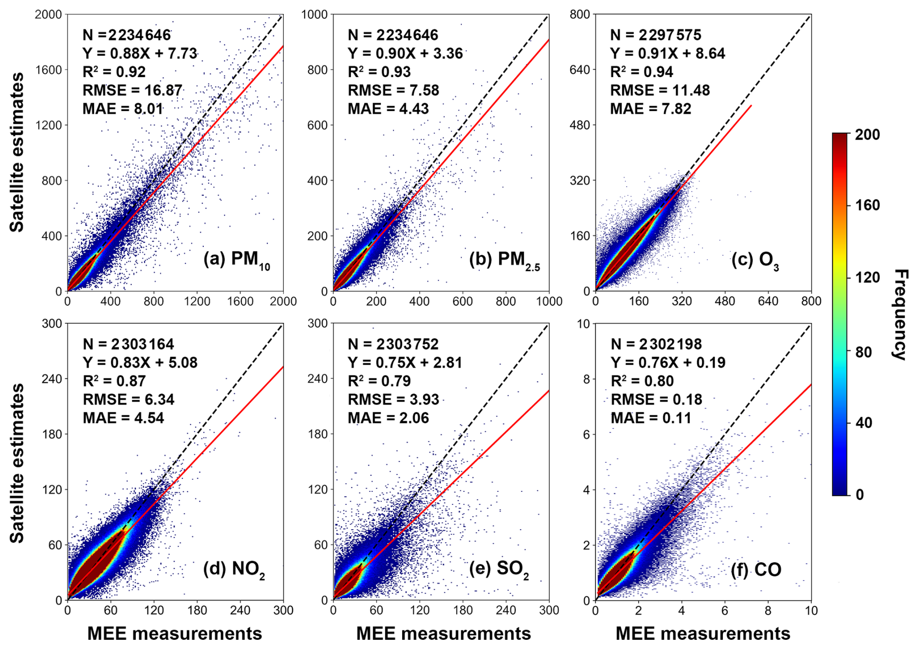
Figure 1 Overall accuracy of daily air pollutant estimates across China. Density scatter plots of satellite-derived daily gapless 1 km concentrations of ambient air pollutants – (a) PM₁₀ (µg m⁻³), (b) PM_2.5 (µg m⁻³), (c) O₃ (µg m⁻³), (d) NO₂ (µg m⁻³), (e) SO₂ (µg m⁻³), and (f) CO (mg m⁻³) – using the unified four-dimensional spatiotemporal deep forest (4D-STDF) model against ground-based measurements from all Ministry of Ecology and Environment (MEE) monitoring stations across China from 2019 to 2022, based on the sample-based 10-fold cross-validation approach. The black dashed lines represent the 1:1 reference line, while the red lines indicate the best-fit lines derived from linear regression.

Furthermore, year-specific validation demonstrates stable model performance over time, showing consistent sample-based CV-R² (RMSE) values during 2019–2022, ranging from 0.89–0.93 (12.51–20.21 µg m⁻³) for PM₁₀, 0.93–0.94 (6.40–8.79 µg m⁻³) for PM_2.5, 0.93–0.95 (10.11–13.59 µg m⁻³) for O₃, 0.86–0.87 (5.80–7.19 µg m⁻³) for NO₂, 0.76–0.81 (3.13–4.87 µg m⁻³) for SO₂, and 0.75–0.82 (0.16–0.20 mg m⁻³) for CO, indicating consistent reliability despite interannual variations in emissions and meteorology. In addition, the number of monitoring stations shows a moderate increase over time, ranging from 1474 to 1896 (Fig. S4), while the spatial distribution remains broadly stable, ensuring that interannual model stability is not confounded by changes in sampling density or spatial coverage.

At the regional scale (Fig. S5), both pollutants show strong performance, with sample-based CV-R² (slope) exceeding 0.93 (0.90) in both Northern and Southern China, and RMSE (MAE) ranges from 5.45–9.42 (3.68–5.26) µg m⁻³ for PM_2.5 and 10.84–11.78 (7.33–8.18) µg m⁻³ for O₃. At the city scale, Wuhan also demonstrates high accuracy, with CV-R² of 0.91 (slope = 0.91) for PM_2.5 and 0.94 (0.91) for O₃, along with average RMSE (MAE) values of 7.12 (5.05) and 12.71 (8.95) µg m⁻³, respectively. These results confirm the model's robustness across spatial scales, including its applicability to fine-scale urban analyses.

3.2 Impacts of abrupt emission changes on air quality

Using machine learning, we derived daily, gapless 1 km maps of six ambient air pollutants across China from satellite observations, providing spatially continuous estimates at each location and for each day, particularly in regions lacking ground-based measurements. Figure 2 presents a representative example on 1 January 2020, illustrating pronounced pollutant-specific spatial heterogeneity. Particulate matter exhibits strong regional clustering, with PM₁₀ showing elevated concentrations in arid and semi-arid regions of northwestern China, largely influenced by natural dust emissions and surface wind erosion, while PM_2.5 displays prominent hotspots over major urbanized and industrialized regions such as the North China Plain, the Fenwei Plain, and the Sichuan Basin. These PM_2.5 enhancements are closely associated with intensive anthropogenic emissions and unfavorable meteorological conditions during winter, including shallow boundary layers and weak ventilation, which promote pollutant accumulation.

In contrast, gaseous pollutants exhibit distinct spatial patterns that reflect differences in emission sources and chemical lifetimes. NO₂ exhibits strong urban-scale gradients and is tightly linked to traffic and industrial combustion sources, whereas SO₂ concentrations are generally low nationwide due to effective emission control policies, with residual enhancements confined to localized industrial regions. CO presents a relatively homogeneous spatial distribution owing to its longer atmospheric lifetime and regional transport. O₃ shows higher concentrations in western and high-altitude regions, while remaining lower in eastern urban areas during winter, reflecting weaker photochemical production and enhanced NO titration. Together, these results highlight the ability of high-resolution, gapless datasets to capture multi-scale characteristics of air pollution and their underlying drivers across China.

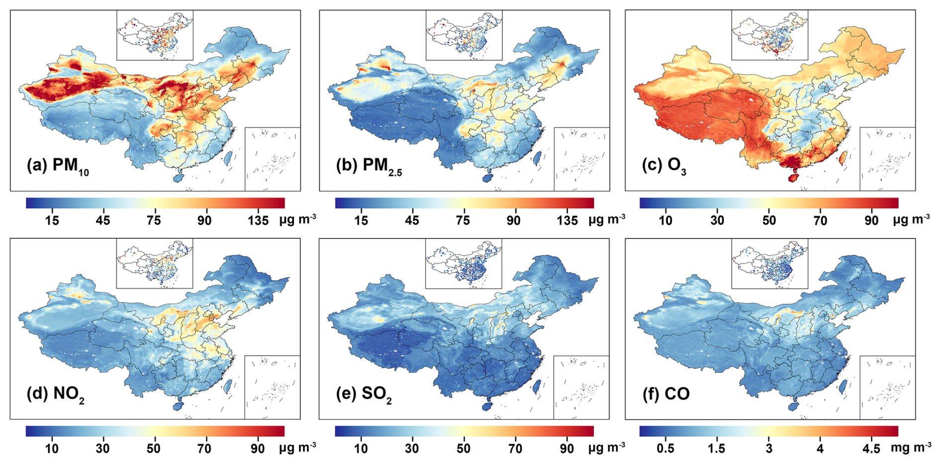
Figure 2 Example of daily 1 km gapless air quality datasets in China. A typical example of (a–f) satellite-derived (horizontal resolution = 1 km) gapless surface (a) PM₁₀ (µg m⁻³), (b) PM_2.5 (µg m⁻³), (c) O₃ (µg m⁻³), (d) NO₂ (µg m⁻³), (e) SO₂ (µg m⁻³), and (f) CO (mg m⁻³) compared with ground measurements on 1 January 2020 in China (inserted upper-middle maps).

These high-resolution AQ datasets enable a detailed examination of short-term pollutant responses to abrupt emission changes (Fig. 3). During the period of stringent emission reductions, marked by elevated values of the Oxford Coronavirus Government Response Tracker (OxCGRT) index in 2020 (Hale et al., 2021), most pollutants exhibited substantial declines, although the magnitude and temporal response varied markedly among species. The Individual Air Quality Index (IAQI) for PM_2.5 showed a sharp decline of 30 % over 22 d, while PM₁₀ decreased by 15 %, taking twice as long – 47 d – to return to normal levels. NO₂ experienced the largest drop, dropping by 32 % over a 52 d response period, while SO₂ and CO demonstrated moderate reductions of 21 % and 19 % over 45 and 25 d, respectively, driven by substantial cuts in anthropogenic emissions from transportation and industrial sources (Wei et al., 2023a, 2022b) In contrast, O₃ concentrations increased by 18 % and exhibited the fastest rebound time (17 d), largely attributable to the substantial reduction in nitrogen oxides (NO_x) emissions under a VOC-limited (NO_x-saturated) chemical regime across much of eastern China (Liu et al., 2021; Wei et al., 2022a). Overall, the Average Air Quality Index (AAQI) declined by 17 % during the most stringent reduction period, indicating widespread improvements in air pollution conditions across China.

During the subsequent emission recovery phase, pollutant-specific responses varied considerably. Approximately half of the pollutant species showed rebounds consistent with a partial resumption of anthropogenic emissions. NO₂ increased most notably, rising by 25 % relative to the reduction phase, reflecting the recovery of traffic and industrial activities. PM₁₀ increased by 16 %, influenced by spring dust events and renewed human activities. O₃ exhibited a slight increase of 1 %, highlighting the continued complexity of ozone formation driven by changes in precursor emissions, particularly NO_x. In contrast, PM_2.5 decreased marginally by 1 %, suggesting more persistent improvements, while SO₂ and CO decreased by 3 % and 8 %, respectively, indicating sustained control of primary emissions. Overall, the AAQI increased by 10 % during the recovery phase, reflecting a partial decline in air pollution conditions; however, conditions remained better than pre-reduction levels, with the aggregated indicator still 9 % lower on average, particularly for PM_2.5 (31 % reduction) and its major precursors (16 %–26 % reductions). These results suggest that although some benefits diminished as emissions resumed, structural reductions and ongoing policy measures contributed to lasting improvements in air quality.

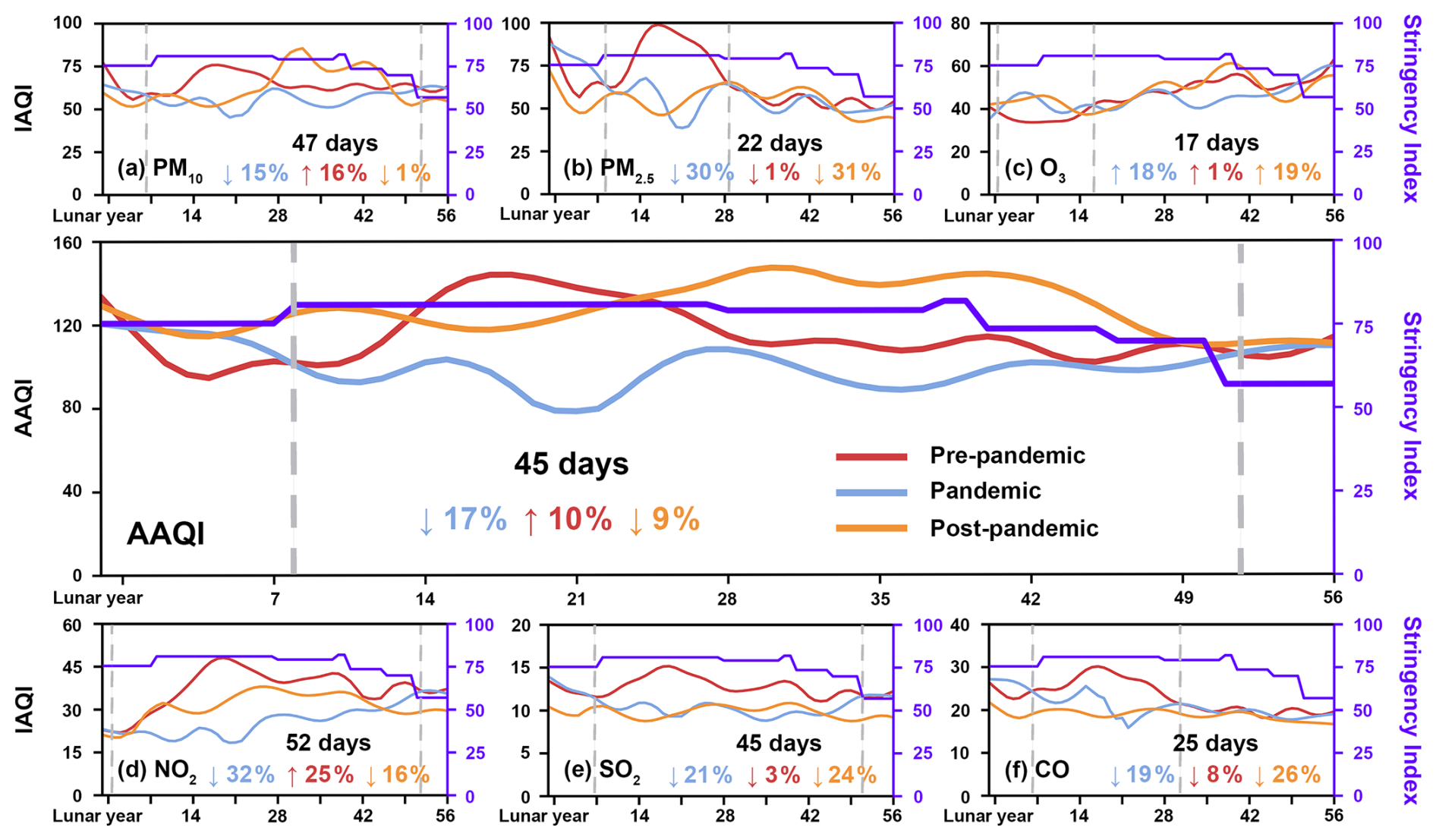
Figure 3 Response of air quality to abrupt emission reductions and subsequent recovery in China. Time series of daily Aggregated Air Quality Index (AAQI) and Individual Air Quality Index (IAQI) (colored lines) for (a) PM₁₀, (b) PM_2.5, (c) O₃, (d) NO₂, (e) SO₂, and (f) CO, along with the Oxford Coronavirus Government Response Tracker (OxCGRT) stringency index (purple lines) as a proxy for emission reduction intensity during the pre-reduction (2019), reduction (2020), and recovery (2021–2022) periods. The data were fitted via Seasonal-Trend Decomposition using the Locally Estimated Scatterplot Smoothing (STL) method. Gray dashed lines indicate the periods of most stringent emission reductions, with response durations (in days) labeled in black. Blue, red, and orange numbers represent the relative changes (%) in AAQI and each IAQI for reduction vs. pre-reduction, recovery vs. reduction, and recovery vs. pre-reduction comparisons, respectively.

During the period of stringent emission reductions, Wuhan, a major urban center with intensive anthropogenic activities, experienced more pronounced and rapid air quality changes than the national average (Fig. 4). PM_2.5 and PM₁₀ levels declined by 37 % and 34 %, respectively, with shorter response times of 35 and 38 d, indicating a stronger and faster particulate matter response to abrupt emission decreases. In contrast, O₃ levels increased sharply by 73 %, about four times the national average, reflecting an intensified ozone formation response under substantially reduced NO_x emissions. NO₂ exhibited the largest decrease (47 %) and the longest rebound period (65 d), consistent with the strong suppression of traffic and industrial emissions in the city. SO₂ and CO experienced moderate declines of 28 % and 12 %, respectively, with response times 2.3–2.4 times shorter than national averages. Overall, the AAQI in Wuhan decreased by 26 % over an average recovery period of 61 d. Notably, the end of this recovery period, identified from satellite observations, closely matched the timing of the city's emission control easing, differing by only ∼5 d, demonstrating the capability of space-based measurements to capture city-scale responses to emission interventions.

During the subsequent emission recovery phase, Wuhan's ambient air pollution levels partially rebounded, with NO₂ and PM₁₀ increasing by 58 % and 35 %, respectively, approximately 2.2–2.3 times the corresponding national averages. PM_2.5 levels also rose by 24 %, contrasting with the slight national decline. In comparison, O₃ exhibited a modest increase of 6 %, while SO₂ and CO continued to decrease at rates similar to national trends. Consequently, the composite index increased by 21 %, reflecting the partial resumption of urban activities. Compared with national patterns, Wuhan experienced more pronounced and faster reductions in particulate matter and NO₂ during the emission reduction phase, a substantially larger O₃ enhancement, and a stronger rebound in NO₂ during the recovery phase, highlighting the effects of stricter local emission controls followed by a rapid return of anthropogenic emissions. Despite this rebound, overall air pollution conditions in Wuhan remained improved relative to pre-intervention levels: except for O₃, which increased by 69 %, all other pollutants decreased by 10 %–21 %, resulting in an overall AAQI reduction of 11 %. These results indicate that, although emissions partially recovered, lasting air quality improvements persisted following the targeted emission control measures.

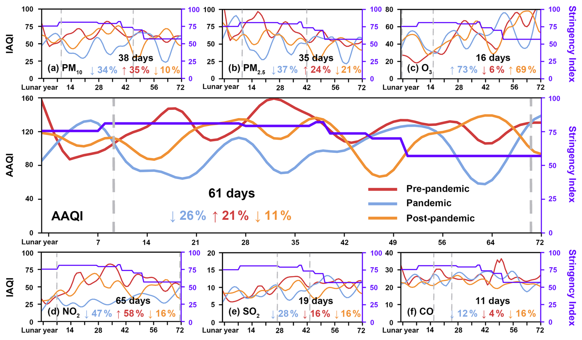
Figure 4 Response of air quality to emission reduction and recovery in Wuhan. Time series of daily Aggregated Air Quality Index (AAQI) and Individual Air Quality Index (IAQI) (colored lines) for (a) PM₁₀, (b) PM_2.5, (c) O₃, (d) NO₂, (e) SO₂, and (f) CO, along with the Oxford Coronavirus Government Response Tracker (OxCGRT) stringency index (purple lines) as a proxy for emission reduction intensity during the pre-reduction (2019), reduction (2020), and recovery (2021–2022) periods in Wuhan, Hubei province, China. The data were fitted via Seasonal-Trend Decomposition using the Locally Estimated Scatterplot Smoothing (STL) method. Gray dashed lines indicate the periods of most stringent emission reductions, with response durations (in days) labeled in black. Blue, red, and orange numbers represent the relative changes (%) in AAQI and each IAQI for reduction vs. pre-reduction, recovery vs. reduction, and recovery vs. pre-reduction comparisons, respectively.

3.3 Fine-scale variations in air quality across the domain

During the most stringent emission reduction period, only 13 % and 9 % of inhabited areas (population density >1 person km⁻²) and counties experienced an increase in PM₁₀ compared to pre-reduction levels (Figs. 5a and S6a), primarily in the desert-dominated northwestern regions affected by enhanced dust events. In contrast, PM_2.5 decreased in 74 % (76 %) of inhabited areas (counties), particularly across the densely populated Northern China Plain, with reductions exceeding 50 %. Pronounced declines in NO₂, SO₂, and CO were observed in 92 % (98 %), 85 % (90 %), and 72 % (87 %) of inhabited areas (counties), respectively, with the largest reductions occurring in urbanized regions of eastern China, especially Wuhan city, reflecting substantial suppression of direct emissions from transportation and industry. O₃ levels, conversely, increased in 76 % (84 %) of inhabited areas (counties), consistent with the spatial reduction of NO₂, which promotes ozone formation under a VOC-limited chemical regime. Overall, atmospheric conditions improved markedly, with 73 % of inhabited areas and 87 % of counties showing decreases in the Aggregated Air Quality Index (AAQI).

During the recovery period, fine-scale air quality patterns exhibited pronounced heterogeneity compared to the reduction period (Figs. 5b and S6b). PM₁₀ increased in 87 % (90 %) of inhabited areas (counties), particularly in Northern and Southwestern China, while PM_2.5 worsened in approximately half of the domain (49 % and 52 % of inhabited areas and counties), mainly in urbanized southeastern regions, including the Yangtze and Pearl River Deltas. NO₂ experienced the largest increase, affecting 90 % of inhabited areas and 96 % of counties, including rural and less industrialized regions. This trend was particularly evident in Hubei province and surrounding areas, where increases exceeded 50 %, reflecting the resumption of construction, transportation, and industrial activity. Moderate increases in SO₂ and CO (47 % and 18 % of inhabited areas, and 48 % and 23 % of counties) were primarily observed in specific industrial regions, suggesting a rebound in coal-dependent industries and partial relaxation of emission controls. O₃ rose in 55 % (48 %) of inhabited areas (counties), particularly in southern regions, likely due to high solar radiation and elevated precursor concentrations. While western regions generally experienced continued air quality improvements, central and eastern China saw noticeable declines. Overall, 72 % of inhabited areas and 70 % of counties showed composite index increases, highlighting the impact of emission recovery on ambient air pollution levels.

Comparing the recovery period to pre-reduction levels (Figs. 5c and S6c), PM₁₀ worsened in 49 % (43 %) of the domain (counties), particularly in central-northern and southern regions, while PM_2.5 IAQI increased in 26 % (24 %) of areas (counties), mainly in densely populated and industrialized southern regions, reflecting the influence of resumed human activities. NO₂ increased in 32 % (17 %) of inhabited areas (counties), while SO₂ and CO showed smaller increases (16 % (8 %) and 13 % (5 %), respectively), indicating that emission controls on vehicles and certain industrial sectors remained effective in many areas. In contrast, O₃ rose sharply in 87 % and 92 % of inhabited areas and counties, particularly in southern and southeastern China, suggesting that elevated precursor concentrations (NO_x and VOCs) and favorable meteorological conditions enhanced ozone formation. Overall, air quality improved in 53 % of inhabited areas and 66 % of counties relative to pre-reduction levels, especially in densely populated central and eastern regions, although other regions experienced localized declines in air pollutant concentrations.

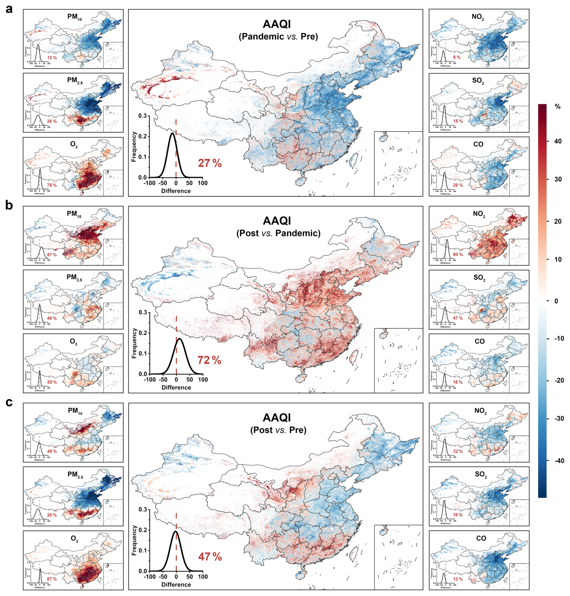
Figure 5 Fine-scale changes in air pollution across different emission-change eras in China. Spatial distributions of relative differences (%) in the Aggregated Air Quality Index (AAQI) and Individual Air Quality Index (IAQI) for PM₁₀, PM_2.5, O₃, NO₂, SO₂, and CO during the most stringent emission reduction periods, compared across three periods – (a) reduction vs. pre-reduction (2020 vs. 2019), (b) recovery vs. reduction (2021–2022 vs. 2020), and (c) recovery vs. pre-reduction (2021–2022 vs. 2019). Results are presented at 1 km² resolution for inhabited areas (population density >1 person km⁻²) across China. Lower-left plots display frequency histograms, with red numbers indicating the percentage of pixels showing deteriorated air quality due to emission recovery.

3.4 Changes in polluted days across the pandemic

Leveraging the daily, gapless air pollutant dataset, we assessed changes in the number of days at different AAQI levels during the first quarter (January–March), which typically experiences severe pollution in China. For example, 40 % (55 %), 34 % (44 %), and 33 % (48 %) of inhabited areas (counties) experienced unhealthy air quality (AAQI >100) for half of the quarter during the pre-reduction, reduction, and recovery periods, respectively (Figs. 6 and S7). Central and eastern China were particularly affected, with pollution exposure frequency exceeding three-fourths of the quarter. Compared to the pre-reduction period (Fig. S8), “Good” days (AAQI <50) increased in 12 % and 38 % of inhabited areas and counties, primarily in southern China, while “Moderate” days (AAQI = 51–100) increased in 72 % and 86 % of areas, mostly in central and eastern regions. More notably, “Unhealthy for Sensitive Groups” (AAQI = 101–150) days decreased in 66 % (62 %) of inhabited areas (counties), especially in central and southeastern China, while reductions in “Unhealthy” (AAQI = 151–200) and “Very Unhealthy” days reached 85 % (86 %) and 93 % (91 %), with hotspots in the North China Plain. Overall, healthy (AAQI <100) days increased in 76 % and 87 % of inhabited areas and counties (Figs. 6d and S7d), reflecting widespread improvement in ambient air pollution conditions during the emission reduction period.

During the recovery period, “Moderate” days showed a mixed pattern, with increases in northern China but decreases in southern and eastern regions (amplitude >20 %), resulting in an overall increase in 65 % of inhabited areas and 58 % of counties (Fig. S9). In contrast, higher pollution levels – “Unhealthy for Sensitive Groups” and “Unhealthy” days – substantially increased in 59 % (68 %) and 50 % (72 %) of areas, mainly in central and southern China, consistent with the partial resumption of anthropogenic emissions. “Good” and “Very Unhealthy” categories showed minimal changes, whereas “Hazardous” days (AAQI = 301–500) increased in 57 % (50 %) of inhabited areas (counties). These patterns indicate an overall deterioration in air pollution conditions during emission recovery (Figs. 6e, S7e), with unhealthy days (AAQI >100) rising in 63 % and 71 % of inhabited areas and counties.

Comparing the recovery to the pre-reduction period (Fig. S10), “Good” days remained similar to the reduction period, with minimal changes in southern regions. “Moderate” days increased in 63 % and 73 % of inhabited areas and counties, with widespread growth across central and southern China, especially in Hubei and surrounding areas, while declines were observed in southern provinces such as Guangdong and Guangxi. Continuous reductions were observed in “Unhealthy for Sensitive Groups,” “Unhealthy,” and “Very Unhealthy” days across 52 % (43 %), 73 % (68 %), and 82 % (79 %) of areas (counties), particularly in the Shandong Peninsula and nearby regions. Meanwhile, “Hazardous” days showed minor spatial changes (<5 %). These results suggest that, although emission levels partially recovered, overall air quality has generally improved relative to pre-reduction levels (Figs. 6f, S7f), with a clear north–south contrast – increasing healthy days in northern China but decreasing in southern regions (65 % vs. 35 % of inhabited areas, 73 % vs. 27 % of counties).

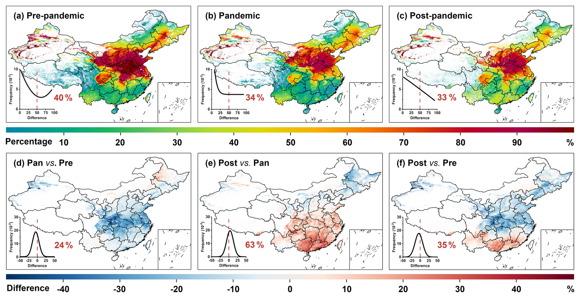
Figure 6 Changes in unhealthy air days across different emission-change eras in China. Spatial distribution of the percentage of days exceeding unhealthy air quality levels (i.e., falling outside the Good (AAQI = 0–50) and Moderate (51–100) categories) during the first quarter (January–March) for the (a) pre-reduction (2019), (b) reduction (2020), and (c) recovery (2021–2022) periods, along with their differences (%) for the following comparisons: (d) reduction vs. pre-reduction, (e) recovery vs. reduction, and (f) recovery vs. pre-reduction. Results are presented at 1 km² resolution for inhabited areas (population density >1 person km⁻²) across China.

3.5 Drivers of major air pollutant changes with XAI

Using eXplainable Artificial Intelligence (XAI), we examined the drivers of changes in PM_2.5 and O₃ concentrations across the pre-reduction (2019), reduction (2020), and recovery (2021–2022) periods. For PM_2.5, population-weighted concentrations declined by 32 % during the reduction period, primarily driven by a 22 % decrease in anthropogenic emissions (Fig. 7a). Sharp emission reductions from industrial activities and transportation led to marked decreases in particulate matter and its precursors. Meteorological conditions contributed a secondary yet important role, accounting for an additional 10 % reduction through enhanced dispersion and increased precipitation. During the recovery period, PM_2.5 stabilized at 40.5 µg m⁻³, with minor changes attributed to meteorology (1 % reduction) and a modest rebound in anthropogenic emissions (4 % increase). These results highlight the dominant role of human-driven emissions in controlling PM_2.5 levels, even as air quality improvements persisted post-reduction.

For O₃, the response differed: during the reduction period, population-weighted concentrations increased by 18 % relative to pre-reduction levels, largely due to meteorological factors (15 %) and partially to emission changes (3 %) (Fig. 7b). This increase reflects the complex photochemical response to reduced NO_x emissions during lockdowns: Lower NO_x emissions during the reduction period decreased O₃ titration in urban areas, resulting in higher ambient O₃ through nonlinear photochemical processes. During the recovery period, O₃ remained elevated at 84.6 µg m⁻³, with negligible additional contributions from meteorology or anthropogenic emissions. These findings underscore the dominant influence of meteorology on O₃ variations, modulated by chemical responses to emission reductions.

Considering regional differences north and south of the Qinling-Huaihe Line, we conducted separate XAI analyses (Fig. 7c–f). During the reduction period, PM_2.5 changes mirrored national trends, dominated by anthropogenic emission decreases (23 % in northern China and 11 % in southern China), while O₃ variations were primarily meteorology-driven (12 % and 13 %, respectively). In the recovery period, PM_2.5 and O₃ continued to decline in northern China by 5 % and 6 %, with anthropogenic factors dominating, whereas both pollutants increased in southern China. In this region, PM_2.5 increases were driven by both human activities and meteorology, while O₃ rises were largely meteorology-driven, influenced by high temperature and humidity.

At the city scale, Wuhan exhibited distinctive trends (Fig. 7g–h). During the reduction period, PM_2.5 decreased by 37 %, mainly due to human emission reductions (22 %), whereas O₃ increased by 40 %, dominated by meteorological factors. During the recovery period, PM_2.5 rebounded by 26 %, largely driven by meteorology (∼16 %), while O₃ decreased by 5 %, with meteorology again as the primary driver. These XAI results are consistent with traditional Multiple Linear Regression (MLR) analyses (Fig. S11) but provide a more nuanced understanding of nonlinear interactions between pollutants and their drivers at national, regional, and urban scales.

Overall, the results highlight the contrasting responses of O₃ and PM_2.5 to changes in emissions: reductions in primary pollutants yield clear benefits for particulate matter but can lead to increased O₃ through complex photochemistry. This underscores the need for balanced emission control strategies that simultaneously address primary and secondary pollutants, especially in densely populated and industrialized regions. The analysis further shows that while emission reductions can rapidly improve air quality, adaptive regulatory frameworks are essential for sustainable management of both PM_2.5 and O₃.

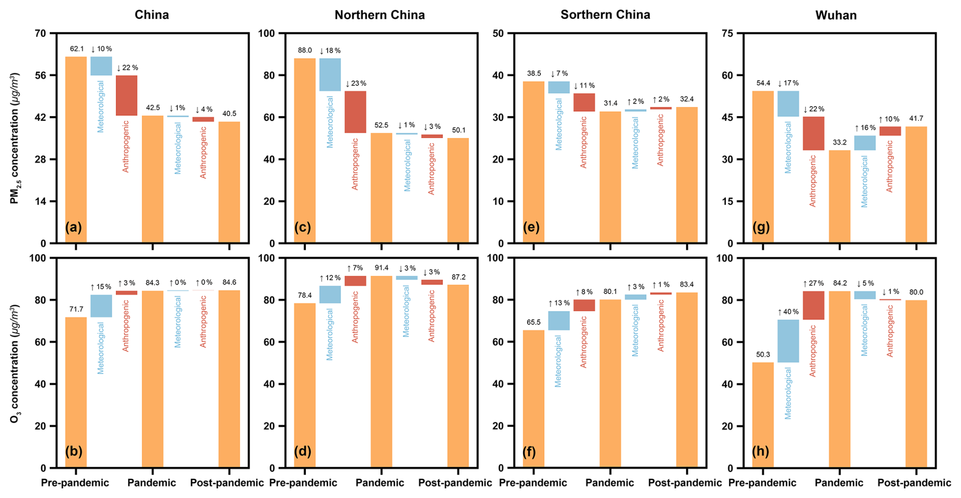
Figure 7 Drivers of air quality variations across different emission-change eras. Influencing factors driving changes in ambient PM_2.5 and O₃ pollution during the most stringent emission reduction period – from the pre-reduction (2019) to the reduction (2020) and recovery (2021–2022) periods – in (a, b) China, (c, d) Northern China, (e, f) Southern China, and (g, h) Wuhan city, Hubei province, using eXplainable Artificial Intelligence (XAI). The blue and red bars represent the contributions of meteorological conditions and anthropogenic emissions, respectively.

4 Conclusions

Previous studies of air quality (AQ) changes in China have largely focused on regional scales, individual pollutants, or the pre-reduction and reduction periods, with uneven ground-monitor coverage limiting fine-scale, nationwide assessment of post-reduction AQ. To address these gaps, we developed a uniform deep learning–based framework to generate a daily, gapless dataset at 1 km² resolution for six conventional air pollutants across China from 2019 to 2022. The resulting daily estimates show strong agreement with over 2.2 million ground-based observations, achieving high accuracy (PM₁₀: CV-R²=0.92, RMSE = 16.87 µg m⁻³; PM_2.5: 0.93, 7.58 µg m⁻³; O₃: 0.94, 11.48 µg m⁻³; NO₂: 0.87, 6.34 µg m⁻³; SO₂: 0.79, 3.93 µg m⁻³; CO: 0.80, 0.18 mg m⁻³), enabling robust multi-pollutant analyses at pixel- and county-scales.

We characterized air quality evolution across the pre-reduction, reduction, and recovery periods, capturing distinct response times to abrupt emission changes (17–47 d). During the reduction period, air quality improved substantially across China, with PM_2.5 and PM₁₀ declining in 76 % and 91 % of counties, NO₂, SO₂, and CO decreasing in 98 %, 90 %, and 87 % of counties, respectively, and overall AAQI improving in 87 % of counties, despite O₃ increases in 84 % of counties. In contrast, the recovery period showed a widespread rebound of air pollution, with NO₂, PM₁₀, and PM_2.5 increasing in 96 %, 90 %, and 52 % of counties, respectively, leading to AAQI deterioration in 70 % of counties as economic activity resumed. Nevertheless, relative to pre-reduction conditions, most primary pollutants (PM₁₀, PM_2.5, NO₂, SO₂, and CO) remained lower in 57 %–95 % of counties, resulting in net AAQI improvements in 66 % of counties, despite a pervasive increase in O₃ across 92 % of counties. These transitions produced pronounced wave-like changes in healthy days (AAQI <100) during the most pollution-sensitive first quarter (January–March), highlighting the combined roles of emission controls, economic recovery, and seasonal processes in shaping post-reduction air pollution levels.

Explainable AI (XAI) analysis revealed that, at the national scale, PM_2.5 variations were dominated by reductions in anthropogenic emissions (22 % during the reduction period), whereas O₃ changes were primarily driven by meteorology (15 % during the reduction period) and nonlinear photochemical responses to NO_x reductions. In Wuhan, PM_2.5 declined during the reduction period primarily due to anthropogenic reductions (∼22 %) but rebounded during recovery, largely driven by meteorological factors (∼16 %), while O₃ remained meteorologically controlled, increasing 40 % during reduction and decreasing 5 % during recovery. Our study provides high-resolution evidence of air quality evolution in China and underscores the need for coordinated, multi-pollutant, mechanism-oriented management strategies that account for both primary and secondary pollutants.