Advancing the quantification of aerosol-cloud interactions with the CALIPSO-CloudSat-Aqua/MODIS record

Aerosol-cloud-precipitation interactions are assessed over the non-polar ocean using more than 11 years of combined Aqua-MODIS, CALIPSO-CALIOP, and CloudSat products. The analysis first shows the benefit of incorporating vertically resolved aerosol extinction coefficient (σ_ext) in aerosol-cloud interactions (ACI) assessments, demonstrating that: σ_ext vertically collocated with the cloud layer (${\mathit{\sigma }}_{\text{ext}}^{\text{CL}}$) correlates best with cloud droplet number concentration (N_d), column-integrated aerosol optical depth (AOD) cannot explain the N_d variability in the extratropics, and the S-shape of the AOD-N_d relationship reported in previous studies is not replicated when using ${\mathit{\sigma }}_{\text{ext}}^{\text{CL}}$ instead of AOD, with a N_d-${\mathit{\sigma }}_{\text{ext}}^{\text{CL}}$ linearity more consistent with in-situ studies over the ocean.

ACI metric, estimated as the log-scale regression between CALIOP ${\mathit{\sigma }}_{\text{ext}}^{\text{CL}}$ and MODIS N_d reveals that the eastern Pacific is the region with the strongest ACI, followed by the Southern Ocean. The susceptibility of clouds to changes in their liquid water path (LWP) and frequency of precipitation followed a 2-step calculation by combining the N_d-${\mathit{\sigma }}_{\text{ext}}^{\text{CL}}$ regression (ACI) with the regression between these macrophysical variables and N_d. LWP susceptibility is negative (LWP decreases with aerosol loading) and statistically significant over the eastern Pacific, eastern Atlantic, and extratropics. In contrast, vast areas of the tropical and subtropical ocean feature negligible changes in LWP with aerosol. Precipitation frequency susceptibility is negative, but the values are only significant over the coastal eastern Pacific and Atlantic. The findings suggest that previous modeling assessments relying on AOD may need to be revisited by taking advantage of the synergy between passive and active sensors.

1 Introduction

Observational estimates of aerosol-cloud interactions (ACI) and cloud adjustments are critical for understanding the role of aerosols and clouds in climate and for testing the ability of models to simulate these susceptibilities. During the past decades, numerous studies have taken advantage of multi-year satellite observations for investigating ACI and cloud rapid adjustments in liquid boundary layer clouds (e.g. Myhre et al., 2007; Quaas et al., 2009; Chen et al., 2014). Although questions remain about the appropriateness of evaluating changes in radiative forcing since pre-industrial times with the use of the current satellite data record (e.g. Mülmenstädt et al., 2024), a more fundamental question to be addressed is whether linear regressions between satellite-derived cloud and aerosol properties capture meaningful physical mechanisms. An encouraging line of evidence is the positive linear correlation observed between satellite aerosol optical depth (AOD) and cloud droplet number concentration (e.g. Quaas et al., 2008), which is generally consistent with airborne observations (e.g. Sorooshian et al., 2019), and in agreement with expectations of the first aerosol indirect effect (that is, increase in cloud droplet concentration with aerosol concentration). This correlation consistency appears to be, in part, attributed to the good skill of satellite retrievals to replicate features observed by ground-based and in-situ platforms, especially over the ocean (e.g. Levy et al., 2013; Painemal et al., 2019; Gryspeerdt et al., 2022). However, fortuitous non-causal aerosol-cloud correlations could impact the interpretation of satellite-based statistics and the way they are used for understanding real physical processes (e.g. Quaas et al., 2020; Rosenfeld et al., 2023). Complexities arise in particular from the use of column-integrated AOD, as its adequacy for representing aerosol concentration or cloud condensation nuclei (CCN) in aerosol activation to cloud droplets have been called into question (Shinozuka et al., 2015; Stier, 2016). This is because AOD (or aerosol index) does not uniquely represent aerosol concentration or CCN concentration, as variations in aerosol composition, particle size distribution, and optical properties can yield the same AOD for different aerosol concentrations. A second limitation is the inability to disentangle the contributions of different aerosol layers to the total AOD, which prevents any meaningful vertical collocation between aerosol and cloud layer (e.g. Jia et al., 2022). These limitations are likely responsible for notable differences between in-situ- and satellite-based aerosol-cloud relationships. For example, the observed logarithmic AOD–N_d relationship from satellites resembles a S-curve: N_d features modest variations with AOD for small AOD values, followed by a rapid linear increase of N_d with AOD, and culminating in N_d values that remain nearly constant for high values of AOD (Gryspeerdt et al., 2016). While it is generally assumed that the insensitivity of N_d to high AOD is likely the result of less aerosol activation in highly polluted environments with substantial CCN availability (e.g. Reutter et al., 2009), the weak N_d–AOD dependency for pristine environments is difficult to interpret without invoking large uncertainties in AOD for regions with small aerosol burden. The weak relationship between N_d and AOD for pristine areas is particularly troubling especially considering the widespread occurrence of regions with low AOD over the ocean, which is precisely where one should expect a substantial occurrence of boundary layer clouds. These results are, again, at odds with multiple field campaigns, which consistently identify linear changes of aerosol concentration with N_d for a wide range of aerosol concentrations (e.g. McFarquhar et al., 2021; Painemal and Zuidema, 2013; Gupta et al., 2022; Zheng et al., 2024).

In addition to limitations in the physical information derived from satellite observations, retrieval artifacts can also impact the interpretation of aerosol-cloud linear regressions. For instance, analysis of passive satellite aerosol and cloud retrievals reveal that biases in AOD can yield underestimations of the N_d-AOD regression of at least 3 % due to aerosol biases in the Level 3 (1°×1°) product (Jia et al., 2022). Moreover, recent studies have warned about biases of aggregating satellite observations without removing pixels more prone to uncertainties (Painemal et al., 2025). To advance in the ACI quantification, Painemal et al. (2020) propose the use of vertically resolved satellite aerosol retrievals, with the objective of isolating the aerosol layer closer in altitude to the cloud layer from the rest of the aerosol column. More specifically, the incorporation of Cloud-Aerosol Lidar and Infrared Pathfinder Satellite Observations (CALIPSO) based aerosol retrievals to the analysis is advantageous for minimizing sensitivities to 3D radiative effects and cloud contamination. Regrettably, studies that make use of spaceborne lidar observations for ACI studies are surprisingly scarce, and global-scale analyses are lacking. Motivated by the proof-of-concept introduced in Painemal et al. (2020), we expand their study by taking advantage of more than 11 years of collocated daytime CALIPSO aerosol properties, MODerate resolution Imaging Spectroradiometer (MODIS) cloud retrievals, and CloudSat precipitation estimates to quantify ACI over the non-polar ocean. This study makes use of aerosol retrievals derived from a physically-based remote sensing algorithm, and thus, no attempts are made to derive aerosol concentration from the CALIPSO observations because we do not have a way to validate the multiple assumptions and approximations needed to compute concentrations from an elastic backscatter lidar. Our overarching objectives are: (a) to investigate the benefits of using vertically resolved aerosol properties and identify regions where the AOD proxy yield meaningful correlations with N_d, and (b) to compute metrics of ACI and cloud susceptibilities over the non-polar oceans.

2 Data and methods

2.1 Satellite products

The dataset for this study comprises daytime observations from Cloud-Aerosol LIdar with Orthogonal Polarization (CALIOP) on the CALIPSO, the CloudSat's Cloud Profiling Radar (CPR), and the MODIS on Aqua, from July 2006 to December 2017, for most of the period for which the 3 satellites flew in formation as a part of the A-Train constellation.

2.1.1 CALIOP

Aerosol retrievals are taken from a research product described in Painemal et al. (2019) that combines CALIPSO attenuated backscattering coefficient with an AOD product derived from the CALIOP's ocean surface return based on the Synergized Optical Depth of Aerosols algorithm (SODA, Josset et al., 2008), described in Painemal et al. (2019). This choice of CALIPSO-based research dataset responds to limitations of the standard CALIPSO product associated with the requirement of the algorithm to detect aerosol layers and categorize them into a limited number of aerosol types, adversely affecting the availability of CALIPSO AOD and extinction coefficient datapoints, and potentially biasing the retrievals especially when aerosol type misclassification occurs (e.g. Kim et al., 2017). The derivation of aerosol extinction coefficient (σ_ext) profiles at 60 m vertical resolution makes use of the attenuated backscattering coefficient and SODA AOD to invert the lidar equation by applying the Fernald-Klett iterative algorithm (Fernald, 1984). More specifically, the lidar equation is solved for the aerosol extinction coefficient and the extinction-to-backscatter ratio, with the latter commonly referred to as lidar ratio. We first start by prescribing a lidar ratio and computing the aerosol extinction coefficient and the corresponding AOD using the CALIPSO attenuated backscattering coefficient as the observational constraint. Next, the retrieved AOD is compared against the SODA AOD and, depending on the magnitude and sign of the difference, the lidar ratio is adjusted and σ_ext and AOD are recalculated (Li et al., 2022). The iteration ends when the retrieved AOD matches its SODA counterpart. Retrieval validations are presented in Painemal et al. (2019) and global statistics of lidar ratio are reported in Li et al. (2022). The lidar ratio (LR) is an important parameter for characterizing aerosols using lidars, and in this study will apply it for providing a coarse characterization of aerosol typing. Alternatively, one could directly use the aerosol typing from the CALIPSO product; however, the specific meaning and interpretation of the clean marine aerosol type have been called into question in Edition 4 (e.g. Toth et al., 2025. CALIPSO Edition 5 was not available at the time this manuscript was submitted for publication).

The CALIPSO-based aerosol products are spatially averaged to the standard 5 km resolution of CALIPSO and integrated into the analysis. To simplify the notation, we refer to the CALIPSO SODA aerosol retrievals as CALIOP-S. To reduce the effect of cloud contamination and signal enhancement near cloud edges (Varnai and Marshak, 2009), we remove from the analysis 5 km spatial averages with CALIOP-S cloud fraction greater than zero. On the issue of aerosol biases near clouds, Christensen et al. (2017) found that the removal of pixels near clouds was an effective way to minimize biases in passive sensor based AOD. However, this finding does not specifically apply to CALIOP because the lidar is nearly insensitive to 3D radiative transfer effects near clouds and aerosol-cloud misclassification. Indeed, the aerosol biases observed in MODIS are ameliorated in CALIOP (Yang et al., 2014). Moreover, Painemal et al. (2020) found that changes in CALIPSO AOD with cloud fraction were only substantial for cloud area fraction >0.9 (90 %), suggesting that a simple screening as a function of area coverage can substantially reduce biases in aerosol retrievals in the vicinity of clouds (see Sect. 2.2).

Cloud top height from CALIPSO version 4.2 (LID_L2_01kmCLay-Standard product) at 1 km resolution is added to the analysis, as it provides accurate detection of cloud top height (H_T). CALIPSO H_T is primarily used for defining the top boundary of the aerosol layer vertically collocated with the cloud. Because the focus of our study is boundary layer clouds (low clouds), we select pixels with H_T<3 km, and compute 5 km spatial averaging, with the corresponding 5 km cloud fraction calculated as the fraction of 1 km low-cloud pixels within the 5 km scanline section.

2.1.2 Aqua MODIS

MODIS cloud properties correspond to pixel-level cloud retrievals obtained from the Cloud and Earth's Radiant Energy System (CERES) Edition 4 product (Minnis et al., 2020). Variables ingested into the analysis include cloud droplet effective radius (r_e), optical depth (τ), temperature, and height (pressure). The estimation of τ and r_e primarily relies on the 0.64 and 3.7 µm MODIS channels, with the 3.7 µm based r_e showing less sensitivity to spatial inhomogeneities and three-dimensional radiative effects than retrievals derived from shorter wavelength channels (Zhang et al., 2012). Liquid water path (LWP) is estimated using the relationship $\text{LWP}=\frac{\mathrm{5}}{\mathrm{9}}\cdot \mathit{\rho }\cdot r_{\mathrm{e}}\cdot \mathit{\tau }$, with ρ denoting the liquid water density. To limit the analysis to low clouds, we only aggregate liquid-phase MODIS pixels (identified by MODIS cloud particle phase product) with cloud tops below 3 km, with pixel-level cloud top height taken from MODIS. N_d is calculated at 1 km (pixel-level) resolution, using the adiabatic formulation described in Painemal (2018) and Grosvenor et al. (2018):

$$\begin{array}{}\text{(1)}& N_{\mathrm{d}}={\mathrm{\Gamma }}^{\mathrm{1}/\mathrm{2}}{\displaystyle \frac{{\mathrm{10}}^{\mathrm{1}/\mathrm{2}}}{\mathrm{4}\mathit{\pi }{\mathit{\rho }}_w^{\mathrm{1}/\mathrm{2}}k}}{\displaystyle \frac{{\mathit{\tau }}^{\mathrm{1}/\mathrm{2}}}{r_{\mathrm{e}}^{\mathrm{5}/\mathrm{2}}}}\end{array}$$

The parameter Γ in Eq. (1) is the adiabatic condensation rate of water vapor with height, which is a function of temperature and pressure (Albrecht et al., 1990). We calculate Γ for each 1 km pixel using MODIS cloud top temperature and pressure. Departures from the adiabatic Γ value are not considered here due to a lack of understanding of how to estimate this adjustment with satellite data. The parameter k is the ratio between the volume radius and r_e and is assumed constant at 0.8 (Martin et al., 1994).

2.1.3 CloudSat Cloud Profiling Radar

CloudSat parameters are obtained from the 2B-GEOPROF Release 05 product. Cloud reflectivity is utilized in our analysis for precipitation detection. To minimize the effect of artifacts and surface echo, we used the CloudSat cloud mask for retaining samples with good and strong echoes (mask value of 30 or 40). The CloudSat maximum radar reflectivity of the cloud column with tops below 3 km (Z_max) is used to categorize the low-cloud precipitation rate for $Z_{\text{max}}>-\mathrm{15}$ dBZ.

2.2 Data matching and additional averaging

The data matching methodology follows Painemal et al. (2020) and is designed to combine datasets with different spatial resolutions, as well as to reduce potential sources of uncertainties that could otherwise impact our analysis. Briefly, the matching is conducted for individual 25 km segments along the CALIPSO ground track (Fig. 1), with the goal of creating a dataset of MODIS, CALIOP, and CloudSat retrieval aggregated to a 25 km resolution. We start by averaging the CALIPSO cloud height to yield a single value per 25 km segment, with values retained for averages constructed with at least 20 % of cloudy observations for the 25 km scanning line to guarantee a significant number of samples in the computation of cloud top height. Next, cloud-free CALIOP-S aerosol extinction coefficients at 5 km resolution are spatially averaged over the same 25 km segment. Lastly, the closest CloudSat CPR pixels to the CALIPSO ground-track, represented by the 25 km segment in Fig. 1 (in blue), are combined to derive a probability of precipitation (POP) defined as the fraction of precipitating pixels of the total cloudy pixels within the segment, with precipitation defined for samples with Z_max greater than −15 dBZ. Note that CloudSat and CALIPSO ground-tracks in Fig. 1 are not identical (e.g., Mace and Zhang, 2014), yet the discrepancy is much less than the 10 km cross-track distance in Fig. 1.

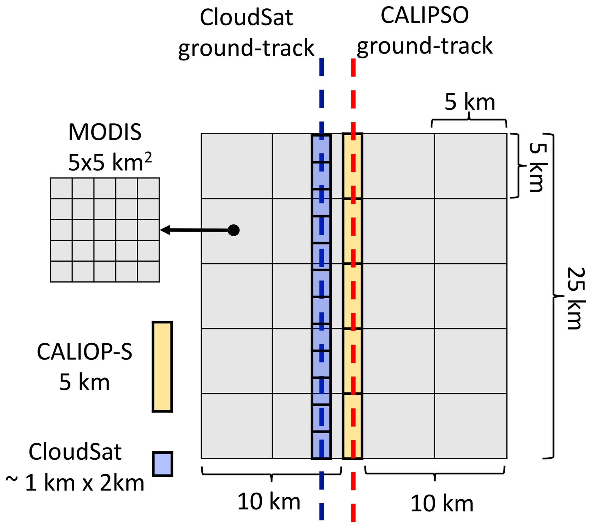
Figure 1 Spatial collocation of the 3 datasets along a 25 km CALIPSO along-track segment. CloudSat footprints are being represented without oversampling. CALIPSO CALIOP-S cross-track footprint is less than 100 m.

Considering that cloud retrievals and N_d come from MODIS, we take a number of steps to reduce retrieval biases. We first match MODIS pixels with the 5 km CALIPSO pixel (Fig. 1, yellow block) by using 5-pixel × 5-pixel MODIS boxes, with 2 boxes east and 2 boxes west of the CALIPSO ground-track (Fig. 1, gray squares). Second, for each of these MODIS data boxes, the 5 km² low-cloud fraction is calculated as the number of liquid phase cloudy points with MODIS cloud top heights of less than 3 km divided by the total number of points. Third, the 20 5×5 MODIS boxes are individually averaged and averaged boxes with cloud fraction greater or equal than 80 % are retained for future averaging. Then, the averaged MODIS boxes centered along the 25 km CALIPSO track segment are finally averaged to produce a single cloud value collocated at the 25 km CALIPSO along-track resolution. At this resolution, averaged MODIS data are used in the analysis when the solar zenith angle is less than 65° and the mean cloud optical depth is greater than 2.0, which helps reduce uncertainties in optically thin clouds (Painemal et al., 2025). Lastly, we only analyzed samples with CALIOP-S AOD greater than 0.05 to reduce uncertainties in the derivation of very low AOD (Painemal et al., 2019).

A final threshold applied to the 25 km aggregated data corresponds to limiting the analysis to MODIS grids with low-cloud fraction equal to or less than 90 %. This upper limit enables the removal of 25 km grids with aerosols fully embedded in cloudy regions, which are more severely affected by aerosol swelling in areas with peaks in humidity (Painemal et al., 2020).

2.3 Aerosol layers

For evaluating the impact of aerosol layers in the ACI quantification, we compute from the 25 km aerosol extinction coefficient horizontal averages, the vertically averaged σ_ext for three 300 m atmospheric layers (Painemal et al., 2020): near-surface (SFC), cloud-level (CL), and free troposphere (FT). Near-surface σ_ext (${\mathit{\sigma }}_{\text{ext}}^{\text{SFC}}$) is estimated as the vertical average value between the height 43 and 343 m above the sea level. Cloud-level average σ_ext (${\mathit{\sigma }}_{\text{ext}}^{\text{CL}}$) is computed as the average for the 300 m layer between 360 and 60 m below the mean cloud top height (25 km CALIPSO H_T). Free tropospheric σ_ext (${\mathit{\sigma }}_{\text{ext}}^{\text{FT}}$) is the 300 m layer average between the altitude 60 and 360 m above the mean CALIPSO cloud top height. The 60 m departure from H_T for the ${\mathit{\sigma }}_{\text{ext}}^{\text{CL}}$ and ${\mathit{\sigma }}_{\text{ext}}^{\text{FT}}$ calculation is intended to minimize the influence of uncertainty in H_T retrievals by limiting the contribution of samples in the free troposphere and boundary layer to the ${\mathit{\sigma }}_{\text{ext}}^{\text{CL}}$ and ${\mathit{\sigma }}_{\text{ext}}^{\text{FT}}$ averages, respectively.

2.4 Satellite susceptibilities

The aerosol-cloud interactions (ACI) metric is defined as the fractional change of N_d in response to the fractional change of aerosols (Eq. 2). In this study, the aerosol component is represented by the layer-averaged σ_ext, and ACI expressed as:

$$\begin{array}{}\text{(2)}& \text{ACI}={\displaystyle \frac{\mathrm{d}\ln \left(N_{\mathrm{d}}\right)}{\mathrm{d}\ln \left({\mathit{\sigma }}_{\text{ext}}\right)}},\end{array}$$

The computation of cloud adjustments (susceptibilities) to aerosols acknowledges the fact that cloud properties (liquid water path and precipitation) are modulated by N_d, which is, in turn, sensitive to variations in aerosol properties (σ_ext). It follows that LWP and precipitation (POP) susceptibilities to aerosol – S_LWP, S_POP respectively – can be expressed as:

$$\begin{array}{}\text{(3a)}& {\displaystyle }{S}_{\text{LWP}}={\displaystyle \frac{\mathrm{d}\ln \left(\text{LWP}\right)}{\mathrm{d}\ln \left({\mathit{\sigma }}_{\text{ext}}\right)}}={\displaystyle \frac{\partial \ln \left(\text{LWP}\right)}{\partial \ln \left(N_{\mathrm{d}}\right)}}\cdot {\displaystyle \frac{\partial \ln \left(N_{\mathrm{d}}\right)}{\partial \ln \left({\mathit{\sigma }}_{\text{ext}}\right)}},\text{(3b)}& {\displaystyle }{S}_{\text{POP}}={\displaystyle \frac{\mathrm{d}\ln \left(\text{POP}\right)}{\mathrm{d}\ln \left({\mathit{\sigma }}_{\text{ext}}\right)}}={\displaystyle \frac{\partial \ln \left(\text{POP}\right)}{\partial \ln \left(N_{\mathrm{d}}\right)}}\cdot {\displaystyle \frac{\partial \ln \left(N_{\mathrm{d}}\right)}{\partial \ln \left({\mathit{\sigma }}_{\text{ext}}\right)}},\end{array}$$

Defining cloud susceptibilities due to cloud microphysical changes as: $S_{\text{LWP}}^{\text{Nd}}=\frac{\partial \ln \left(\text{LWP}\right)}{\partial \ln \left(N_{\mathrm{d}}\right)}$ and $S_{\text{POP}}^{\text{Nd}}=\frac{\partial \ln \left(\text{POP}\right)}{\partial \ln \left(N_{\mathrm{d}}\right)}$. We can simplify the notation and express the overall susceptibility due to aerosols as:

$$\begin{array}{}\text{(4a)}& {\displaystyle }{S}_{\text{LWP}}=S_{\text{LWP}}^{\text{Nd}}\cdot \text{ACI},\text{(4b)}& {\displaystyle }{S}_{\text{POP}}=S_{\text{POP}}^{\text{Nd}}\cdot \text{ACI},\end{array}$$

ACI, $S_{\text{LWP}}^{\text{Nd}}$, $S_{\text{POP}}^{\text{Nd}}$, and are calculated as the linear regression between the natural logarithm of cloud and aerosol properties, following a binning method described in the following sections. For this study, we do not compute cloud fraction susceptibility ($S_{\text{CF}}^{\text{Nd}}=\frac{\partial \ln \left(\text{CF}\right)}{\partial \ln \left(N_{\mathrm{d}}\right)}$) as our CF dependent filtering could impact the susceptibility computations.

3 Results

3.1 Impact of the aerosol layer selection

The three different values of layer aerosol extinction coefficient (${\mathit{\sigma }}_{\text{ext}}^{\text{SFC}}$, ${\mathit{\sigma }}_{\text{ext}}^{\text{CL}}$, and ${\mathit{\sigma }}_{\text{ext}}^{\text{FT}}$) are utilized to determine whether a specific aerosol layer covaries the strongest with N_d. To this end, we compute maps of Spearman linear correlation coefficient (r) for the matched observations using a 5°×5° regular grid. First, we group the control variable (σ_ext) in 20 quantiles, with the goal of determining σ_ext bin sizes common to all 5°×5° regions. We generally favor the use of the Spearman correlation for this study because the metric provides information about the monotonic increase in a relationship and is less affected by outliers than the standard Pearson correlation coefficient. Next, we average N_d as a function of the 20 σ_ext bins. To eliminate spurious results associated with reduced sampling in each 5°×5° grid, we only use binned σ_ext – N_d when they are created with at least five paired samples per bin, and the total number of valid bins is at least 10, totaling at least 50 datapoints for regression calculation. The maps in Fig. 2 depict r for N_d–${\mathit{\sigma }}_{\text{ext}}^{\text{SFC}}$ (Fig. 2a), N_d–${\mathit{\sigma }}_{\text{ext}}^{\text{CL}}$ (Fig. 2b), and N_d–${\mathit{\sigma }}_{\text{ext}}^{\text{FT}}$ (Fig. 2c), with gray areas representing grids with insufficient number of samples or valid bins to perform the calculation. Overall, the analysis shows that N_d correlates the highest with cloud-level σ_ext with overall correlation coefficient greater than 0.7 over vast oceanic regions, except for the tropical Pacific, where the correlations are modest (Fig. 2b). Surface-layer σ_ext is positively correlated to N_d in the littoral regions of South Atlantic, the western Africa, Indian Ocean, and western North Pacific, however, the correlations are weaker than those for N_d–${\mathit{\sigma }}_{\text{ext}}^{\text{CL}}$. The N_d is least correlated to the free tropospheric σ_ext (Fig. 2c), but with a few patches of r>0.5 over the east coast of South America and southern Africa. Overall, the findings in Fig. 2 support the hypothesis formulated in Painemal et al. (2020) and Stier (2016) in that isolating the aerosol layer closer to the cloud deck is central for a more rigorous quantification of aerosol-cloud interactions. For the rest of this study, we will primarily center our attention on the relationship between ${\mathit{\sigma }}_{\text{ext}}^{\text{CL}}$ and other cloud quantities. The corresponding Pearson correlation coefficient (Fig. S1 in the Supplement) reveals a pattern quite similar to r in Fig. 2, with Fig. S1b confirming both that the relationship between N_d and ${\mathit{\sigma }}_{\text{ext}}^{\text{CL}}$ is monotonic and linear.

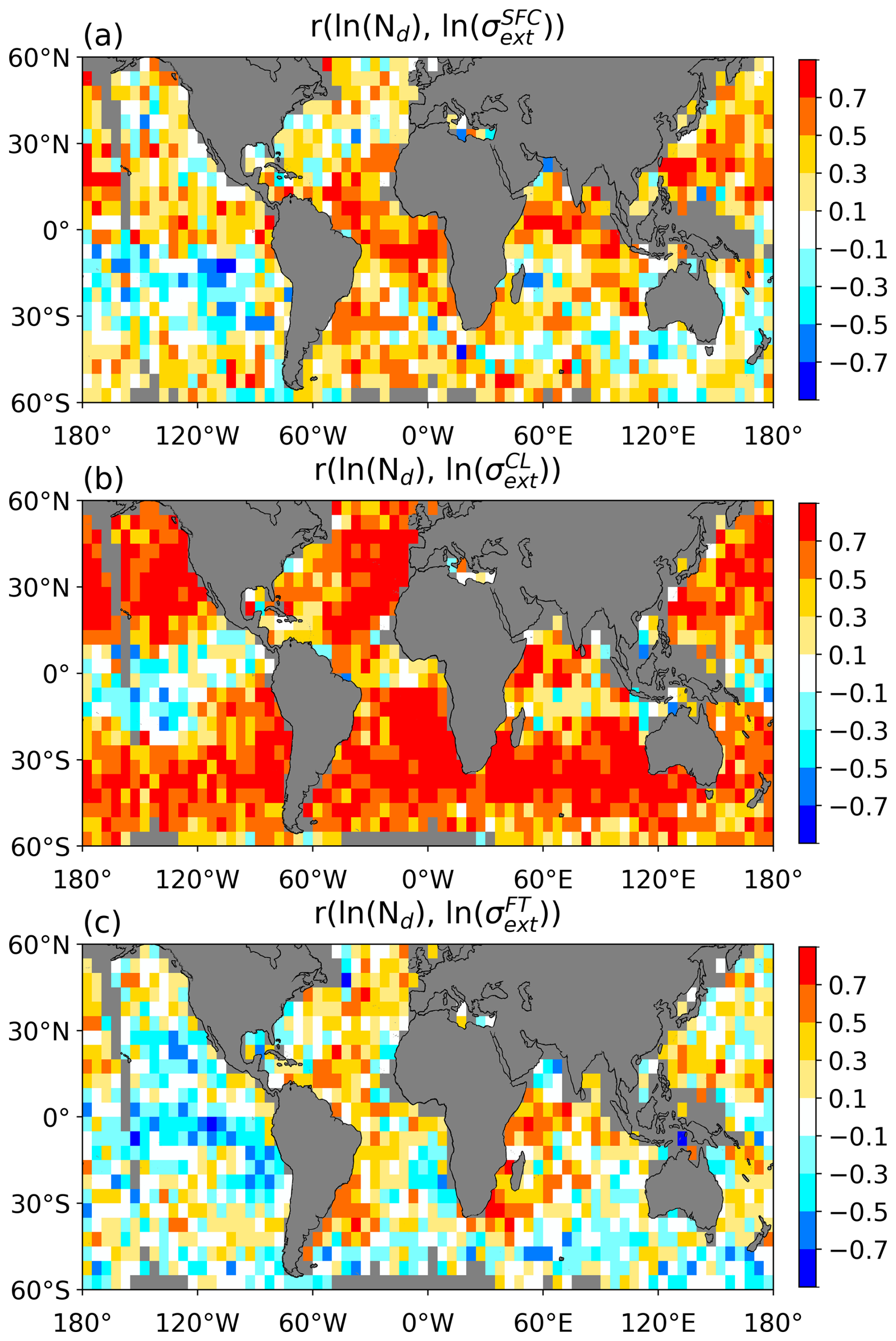
Figure 2 Gridded maps of correlation coefficient between MODIS N_d and (a) surface layer σ_ext (${\mathit{\sigma }}_{\text{ext}}^{\text{SFC}}$), (b) cloud level σ_ext (${\mathit{\sigma }}_{\text{ext}}^{\text{CL}}$), and (c) free tropospheric σ_ext (${\mathit{\sigma }}_{\text{ext}}^{\text{FT}}$). Correlations are estimated after applying the natural logarithm to the variables.

Having demonstrated that the aerosol extinction coefficient adjacent to the cloud-layer altitude is the parameter that best correlates with N_d, we assess the benefits of applying ${\mathit{\sigma }}_{\text{ext}}^{\text{CL}}$ to the analysis relative to the use of standard AOD as a control variable. For this purpose, we consider the relationship between CALIOP-S aerosol retrievals and N_d for five latitudinal bands and compare the aerosol–N_d relationship for the 2 control variables: ${\mathit{\sigma }}_{\text{ext}}^{\text{CL}}$ and AOD. For each regional band, we average N_d as a function of 50 CALIOP-S aerosol bins with equal number of data points. It is noteworthy to mention that because the vertically integrated σ_ext in the CALIOP-S data product is AOD (Painemal et al., 2020), analysis differences can only be attributed to the use of vertically resolved versus vertically integrated quantities, rather than product and algorithm discrepancies. A key characteristic depicted in Fig. 3a is that the shape of the N_d-${\mathit{\sigma }}_{\text{ext}}^{\text{CL}}$ relationship can be generally captured by a linear fit, with some departures for the 10 % smallest aerosol extinction coefficients (<0.01 km⁻¹), which are values within the retrieval uncertainty range (Painemal et al., 2019). Moreover, the strong relationship is observed across all the latitudinal bands, with Spearman correlation coefficients greater than 0.98 and Pearson values ≥0.88, confirming the linearity and monotonicity of the relationship. On the other hand, N_d shows little sensitivity to AOD for specific AOD regions (Fig. 3b). For example, the 40–60° latitude bands exhibit modest changes in N_d with AOD for AOD<0.2 (Fig. 3b, magenta and black), with overall Spearman correlation coefficient of 0.37 (40–60° N) and 0.16 (40–60° S). While the Pearson correlation for these 2 extratropical regions is relatively high (Spearman correlation, r_s>0.53), it indicates that a few outliers for AOD>0.2 account for the overall increase. For other bands (20–40° N and 20° S–20° N), the sensitivity of N_d is modest for AOD>0.2, with variations of less than 10 cm⁻³ in the tropical region (Fig. 3b, blue triangles). In sum, the analysis reveals that either, the N_d-AOD curve is not monotonic, at times governed by outliers with AOD>0.2, and consequently is poorly represented by a linear fit. Moreover, because the flattening of the N_d curve with AOD is not observed in σ_ext, this suggests that the S-shape curve between N_d and AOD reported in a number of studies may not be the manifestation of microphysical processes, rather it reflects the inadequacy of AOD as an aerosol proxy for ACI studies, especially for higher N_d.

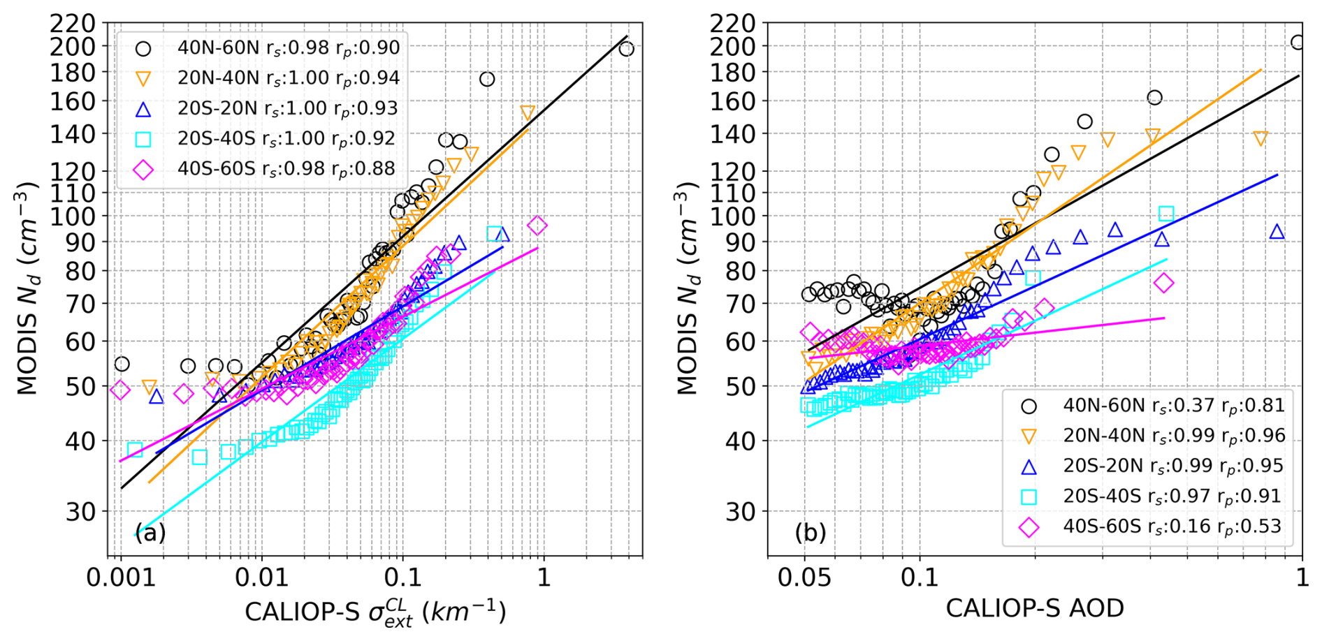
Figure 3 MODIS N_d as a function of (a) CALIOP-S ${\mathit{\sigma }}_{\text{ext}}^{\text{CL}}$ and (b) AOD. The relationships are shown for five latitude bands: 40 to 60° N (black circle); 20 to 40° N (gold inverted triangle); 20° S to 20° N (blue triangle); 20 to 40° S (cyan square); 40 to 60° S (magenta diamond). The linear best fit of each latitude band, represented by the line of corresponding color is estimated from the variables in logarithmic scale. r_s and r_p denotes, respectively, Spearman and Pearson correlation coefficients.

3.2 Aerosol-cloud interactions

Given the benefits of using ${\mathit{\sigma }}_{\text{ext}}^{\text{CL}}$ for studying the impact of aerosols on N_d, we apply Eq. (2) to estimate ACI via the linear regression between N_d and ${\mathit{\sigma }}_{\text{ext}}^{\text{CL}}$. In terms of number of samples (Fig. 4a), the subtropical open ocean features the largest yield (>850) whereas the Southern Ocean and the region north of 45° N show the lowest data availability (<350) due to the lack of aerosol retrievals there, for regions with extensive cloud coverage. Figure 4b shows the ACI map, computed following the same 20-bin methodology and spatial resolution applied to the construction of the 5°×5° correlation maps in Fig. 2. Statistically significant values are positive over most of the non-polar oceans, consistent with the notion that more aerosols drive an increase in cloud droplet number concentrations. The highest fractional changes of N_d with ${\mathit{\sigma }}_{\text{ext}}^{\text{CL}}$ are found in the coastal southeast Pacific, the northeast, and southeast Atlantic. These ACI peaks coincide with the location of subtropical stratocumulus cloud regimes, which have shown the largest sensitivity to changes in their shortwave fluxes due to perturbations in N_d (Painemal, 2018; Zhang and Feingold, 2023). Other regions with high ACI include the northeast Pacific Ocean and the Southern Ocean within the 60° W–140° E zonal band. In contrast, values statistically indistinguishable from zero are found over vast regions in the tropical ocean, where shallow cumulus clouds more frequently occur. It is also noteworthy that regions with high ACI in the southeast Atlantic and eastern Pacific, are also associated with modest precipitation occurrence (Fig. 5). For a more quantitative assessment of the role of precipitation, we compute ACI maps separately for non-precipitating and precipitating clouds. To this end, we define a 25 km segment (Fig. 1) as being non-precipitating if POP<0.05 (<5 %) and precipitating for POP>0.3 (30 %). ACI for precipitating clouds (Fig. 6a) generally features slightly negative values but statistically indistinguishable from the zero slope. In contrast, non-precipitating ACI (Fig. 6b) is similar to that derived irrespective of precipitation in Fig. 4b. Indeed, this similarity highlights that the low ACI values for vast regions over the tropical ocean is not linked to precipitation modulation (in an Eulerian sense).

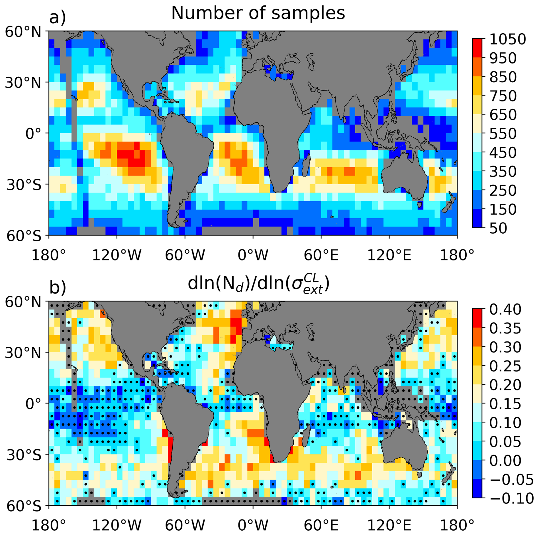
Figure 4 (a) Number of available 25 km samples used for ACI quantification. (b) Gridded map of ACI index ($\mathrm{d}\ln \left(N_{\mathrm{d}}\right)/\mathrm{d}\ln \left({\mathit{\sigma }}_{\text{ext}}^{\text{CL}}\right)$). Black dots indicate grids that are statistically indistinguishable from zero, according to a Student's t test at 95 % confidence level.

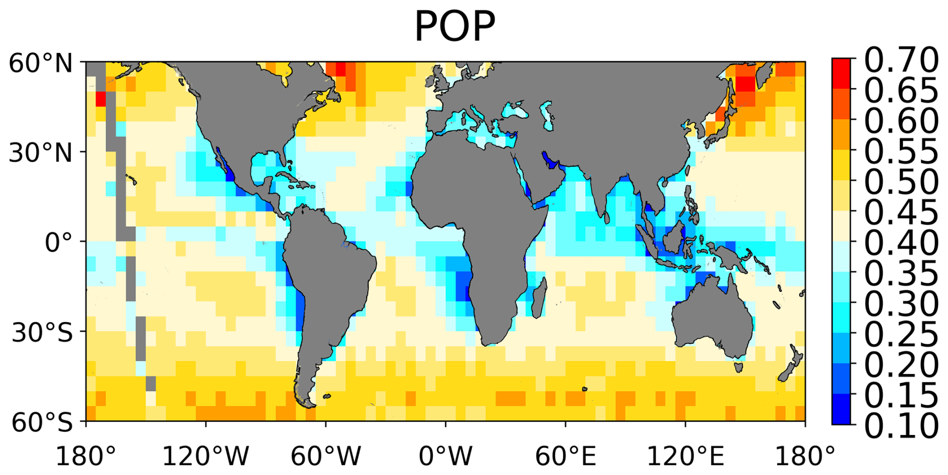
Figure 5 Mean frequency of precipitation occurrence for cloudy observations from CloudSat, with precipitating samples defined as having $Z_{\text{max}}>-\mathrm{15}$ dBZ.

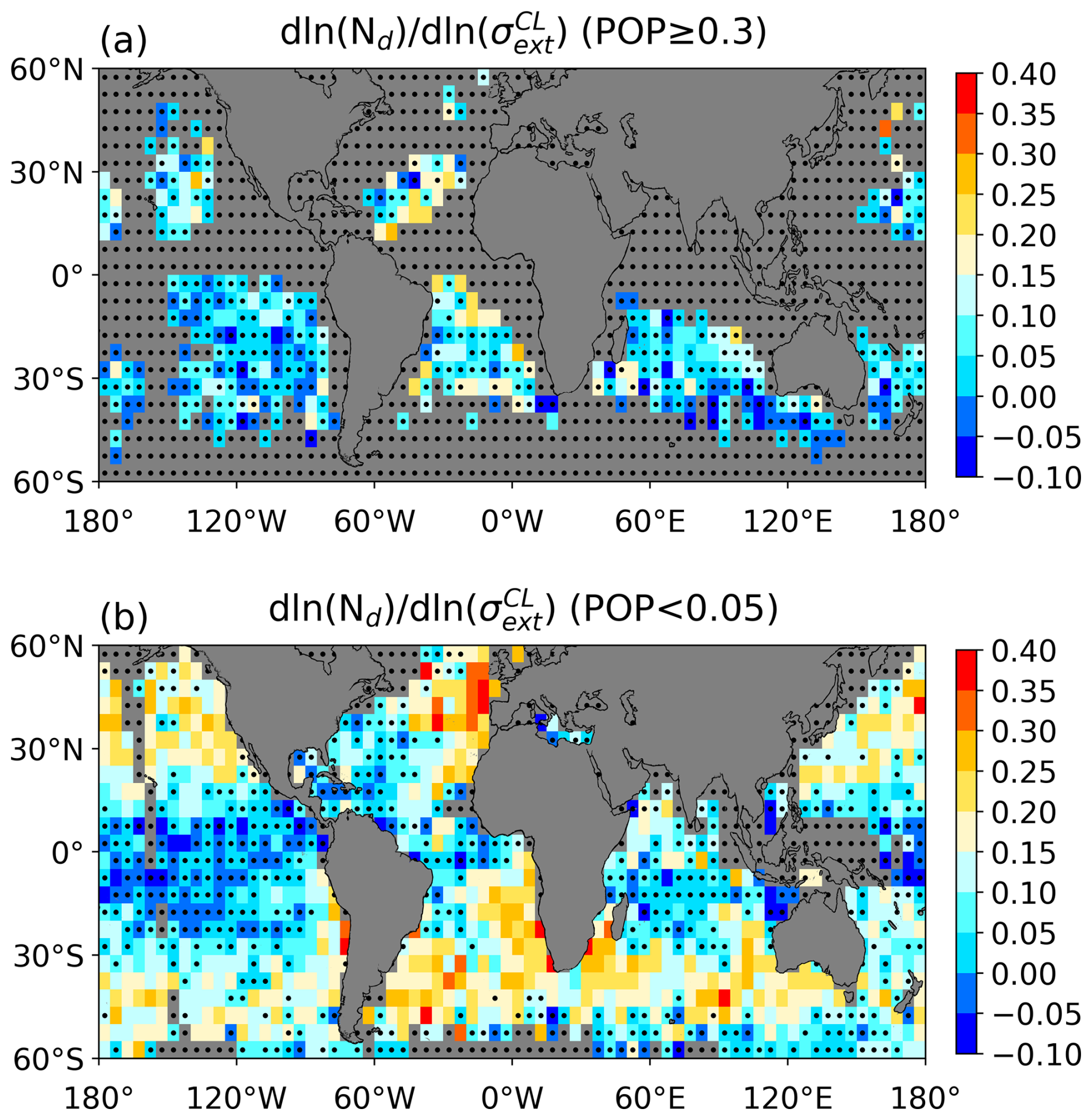
Figure 6 Gridded map of ACI index ($\mathrm{d}\ln \left(N_{\mathrm{d}}\right)/\mathrm{d}\ln \left({\mathit{\sigma }}_{\text{ext}}^{\text{CL}}\right)$). (a) Precipitating (POP<0.05) and (b) non-precipitating samples (POP≥0.3). Black dots indicate grids that are statistically indistinguishable from zero, according to a Student's t test at 95 % confidence level.

3.3 LWP susceptibility

The estimation of susceptibilities follows the regression method used for ACI. Since cloud susceptibilities are the regression between 2 cloud properties, the CF≤0.9 constraint – intended for reducing biases in aerosol retrievals – is no longer needed. We start with the LWP-N_d sensitivity term of Eq. (4a) ($S_{\text{LWP}}^{\text{Nd}}=\frac{\partial \ln \left(\text{LWP}\right)}{\partial \ln \left(N_{\mathrm{d}}\right)}$), as depicted in Fig. 7a. The map reveals two regimes over the ocean: (1) LWP increases with N_d over the tropics, and (2) LWP decreases in the subtropics and extratropics, with minima in high latitudes. This pattern is consistent with the results in Gryspeerdt et al. (2019), although the negative/positive $S_{\text{LWP}}^{\text{Nd}}$ contrast is more striking in our analysis, likely due to the less stringent data filtering applied in our study, which favors a wider dynamic range in LWP than that in Gryspeerdt et al. (2019). A closer inspection of four specific 20°×20° regions with positive and negative signs of $S_{\text{LWP}}^{\text{Nd}}$, uncovers how the LWP dependency on N_d varies for different ranges of LWP (Fig. 8). For the tropical areas (Fig. 8, black circles and magenta triangles), the strong positive LWP-N_d correlation is observed for low values of LWP with N_d. Conversely, the negative correlation in other regions is characterized by larger LWP for low N_d, decreasing to LWP<40 g m⁻² for N_d>100 cm⁻³. It is interesting to note that only when the full non-polar dataset is analyzed (Fig. 8, red), the inverted-V shape emerges. This demonstrates that relationships estimated at global scale should not be interpreted in the context of physical processes and regimes that modulate cloud susceptibilities. This explanation is similar to that in Arola et al. (2022), which postulates that natural heterogeneity can contribute to the misinterpretation of the LWP–N_d relationship.

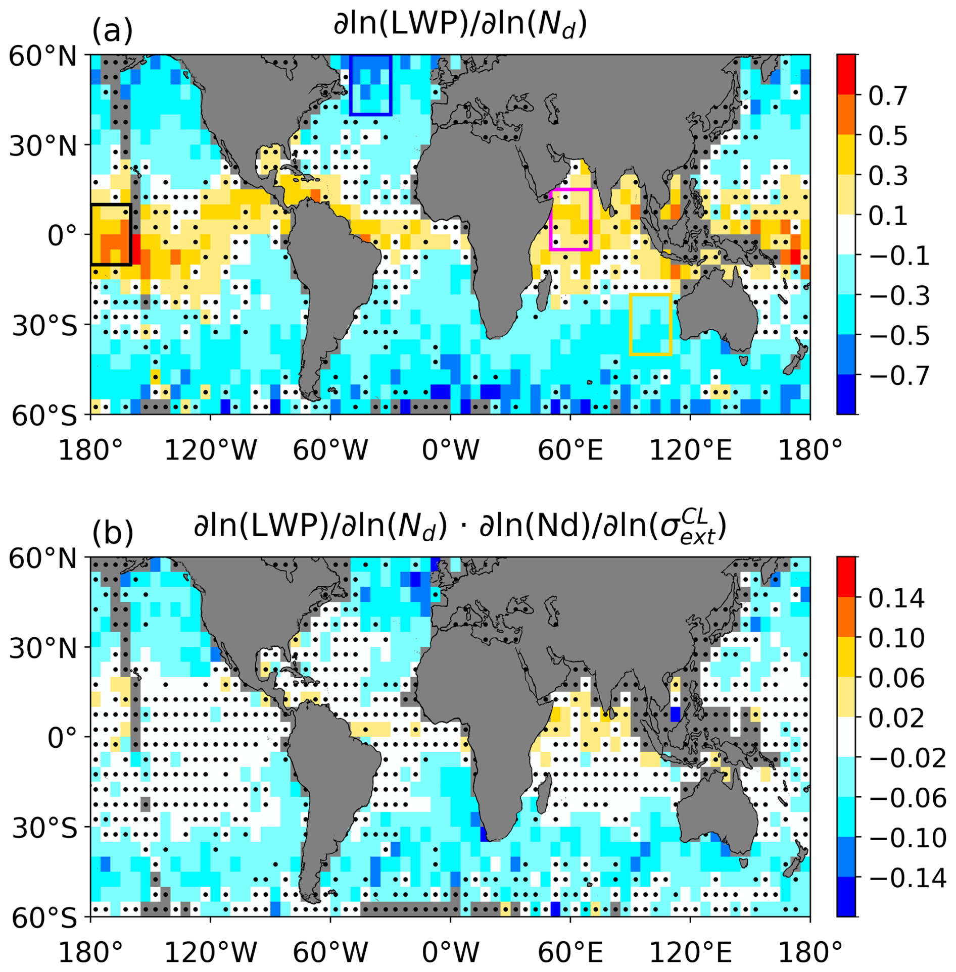
Figure 7 Gridded maps of (a) susceptibility of LWP to N_d or $S_{\text{LWP}}^{\text{Nd}}=\frac{\partial \ln \left(\text{LWP}\right)}{\partial \ln \left(N_{\mathrm{d}}\right)}$; and (b) overall LWP susceptibility to aerosols estimated as $S_{\text{LWP}}=S_{\text{LWP}}^{\text{Nd}}\cdot \text{ACI}$. Black dots in (a) indicate grids that are statistically indistinguishable from zero, according to a Student's t test at 95 % confidence level, whereas dots in (b) represent boxes when at least one metric (ACI or $S_{\text{LWP}}^{\text{Nd}}$) is statistically indistinguishable from zero. The LWP susceptibility computation includes 25 km cloud fraction >0.9 (90 %). The four regions in Fig. 8 are depicted in Fig. 7a with each region highlighted with the same legend color.

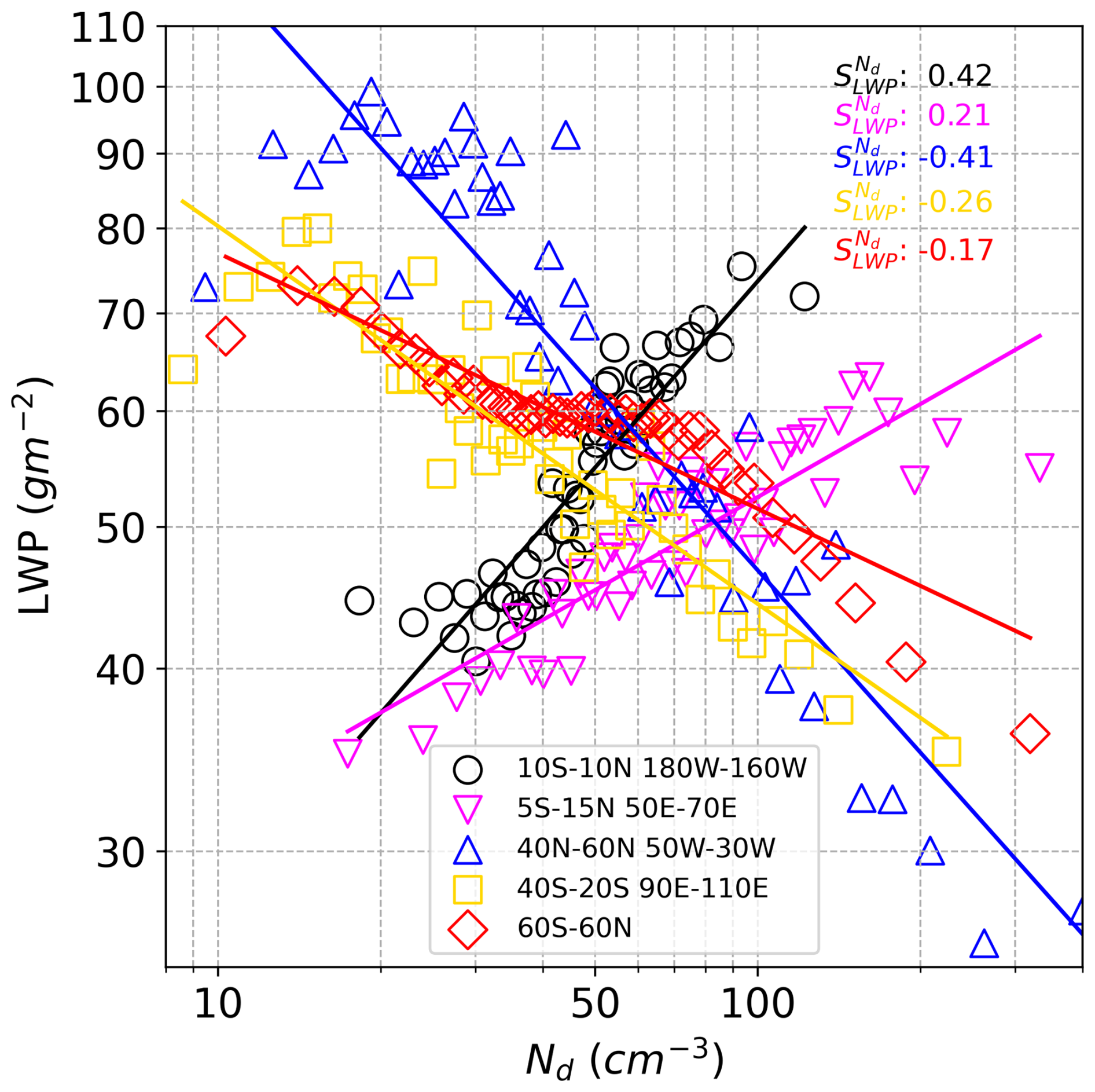
Figure 8 LWP-N_d relationship for 20°×20° regions with opposite sign slope, highlighted in Fig. 7a with the same color code. Central Pacific: 10° S–10° N, 180–160° W (black circles); tropical Indian Ocean: 5° S–15° N, 50–70° E (magenta inverted triangles); north Atlantic: 40–60° N, 50–30° W (blue triangles); and Southern Ocean: 40–20° S, 90–110° E (gold square).

LWP susceptibility S_LWP, is finally estimated as the product between $S_{\text{LWP}}^{\text{Nd}}$ and ACI (Fig. 7b). The S_LWP map features an overall negative susceptibility, indicating that the aerosol effect on LWP is a net reduction in LWP with an aerosol increase. It is also interesting that the susceptibility pattern is mainly driven by extratropical clouds in the Southern Ocean, eastern Pacific and Atlantic oceans. On the other hand, the susceptibility in the tropics and in parts of the subtropical open ocean is negligible.

3.4 POP (precipitation) susceptibility

The first step for estimating precipitation (POP) sensitivity is to quantify the POP-N_d sensitivity ($S_{\text{POP}}^{\text{Nd}}$, Fig. 9a). Due to the lack of precipitating samples and surface clutter in the CloudSat product, it is not possible to consistently estimate $S_{\text{POP}}^{\text{Nd}}$ for all areas. Moreover, when the data yield allows for the estimate of $S_{\text{POP}}^{\text{Nd}}$, the values are insignificant for most oceanic areas (Fig. 9a). For the regions with statistically significant $S_{\text{POP}}^{\text{Nd}}$, the total POP sensitivity to N_d is mostly negative, with the strongest susceptibilities over the eastern Pacific and southeast Atlantic. These regions are also those with statistically significant values of overall precipitation susceptibility due to aerosols (Fig. 9b). For these stratocumulus cloud regimes, the negative susceptibility is consistent with the notion that aerosols suppress precipitation simulated by numerical models (Mülmenstädt et al., 2024).

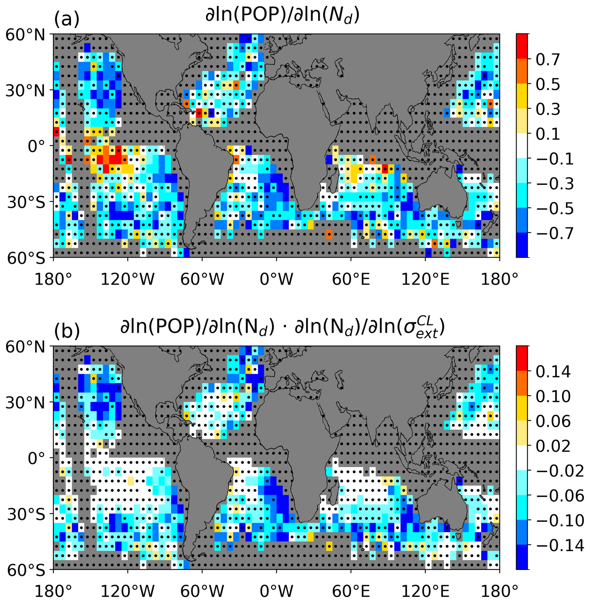
Figure 9 Gridded maps of (a) susceptibility of POP to N_d or $S_{\text{POP}}^{\text{Nd}}=\frac{\partial \ln \left(\text{POP}\right)}{\partial \ln \left(N_{\mathrm{d}}\right)}$; and (b) overall POP susceptibility to aerosols estimated as $S_{\text{POP}}=S_{\text{POP}}^{\text{Nd}}\cdot \text{ACI}$. Black dots in (a) indicate grids that are statistically indistinguishable from zero, according to a Student's t test at 95 % confidence level, whereas dots in (b) represent boxes when at least one metric (ACI or $S_{\text{POP}}^{\text{Nd}}$) is statistically indistinguishable from zero.

4 Discussion

In light of the results presented here, it is pertinent to revisit previous ACI assessments based on Aqua MODIS AOD. For this purpose, we take 5 years of daily Collection 6 MODIS Level 3 (L3) Atmosphere Gridded Product (MYD08_D3) and we compute ACI as ${\text{ACI}}_{\text{AOD}}=\frac{\mathrm{d}\ln \left(N_{\mathrm{d}}\right)}{\mathrm{d}\ln \left(\text{AOD}\right)}$, following the binning methodology used for the CALIOP-MODIS ACI calculations. MODIS L3 ACI map (Fig. 10) features a regional distribution that depart from the MODIS-CALIOP (Fig. 3). This level 3 based analysis partially differs from using pixel-level AOD (Fig. S2) due, likely, to the impact of the data filtering of Sect. 2. An important difference between both ACI estimates is in their magnitude, with MODIS L3 exhibiting values twice as large as those from MODIS-CALIOP. Because the functional relationship between AOD and N_d, and AOD and σ_ext are highly non-linear (Fig. 3b and Painemal et al., 2020), with the disadvantages of using AOD previously discussed, comparing ACI_AOD magnitudes does not provide meaningful information. Instead, our focus is on the interpretation of regional changes relative to the global map. In this regard, a key difference is the negligible ACI_AOD in the extratropics, especially in the Southern Ocean and north of 40° N. This contrasts with the local maximum observed over the same region for the ${\mathit{\sigma }}_{\text{ext}}^{\text{CL}}$-based ACI (Fig. 4). Moreover, except for the region west of Australia, the stratocumulus subtropical regions of the eastern Pacific and Atlantic show modest ACI in the AOD-based calculation, in disagreement with the analysis of Fig. 4 and with in-situ observations (e.g. Kang et al., 2021; Gupta et al., 2022; Sorooshian et al., 2019; Zheng et al., 2024). Figure 10 raises the concern, once again, that AOD-N_d relationship might be misrepresenting ACI and, thus, could misguide modelers about the physical processes that need to be refined, or retained, in models.

Figure 10 Gridded maps of ACI index $\mathrm{d}\ln \left(N_{\mathrm{d}}\right)/\mathrm{d}\ln \left(\text{AOD}\right)$, estimated from MODIS Atmosphere Team (Collection 6) Level 3 daily retrievals.

An aspect not explored in this study is the relationship between aerosol extinction coefficient and aerosol concentration and how it would impact the ACI calculations. While empirical relationships do show a close linear log-scale relationship between boundary layer aerosol concentration and aerosol extinction coefficient (e.g. Shinozuka, et al., 2015) significant regional variations are expected to affect the extinction-to-CCN conversion. An additional difficulty is accounting for the effect of ambient relative humidity in controlling the aerosol hygroscopicity and optical properties (Gasso et al., 2000), which is also dependent on aerosol size and chemical composition, but cannot be characterized with the needed accuracy using satellite data only. Regarding the potential effect of varying regional ambient relative humidity on aerosol extinction, we note that humidity in the boundary layer over the ocean remains on average bounded to values around 85 %, with modest changes across regions (not shown). That is, the narrow range of spatial variability in relative humidity suggests that the ACI patterns described in our study are not explained by humidity driven swelling.

A similar effort of matching aerosol products derived from CALIOP with satellite cloud retrievals was reported in Alexandri et al. (2024). Their study relies on cloud retrievals over Europe from the geostationary sensor The Spinning Enhanced Visible and InfraRed Imager (SEVIRI), and a CCN estimate derived using CALIOP products. Since the estimation of aerosol concentration from an elastic backscatter lidar involves several assumptions (aerosol model, typing, hygroscopic growth, and other empirical approximations), the way multiple uncertainties propagate into the derived product remains to be determined. To circumvent potentially large uncertainties when applying CCN retrieval algorithm, we recommend that future analyses should be framed in terms of the ambient aerosol extinction coefficient. This approach is adopted in an accompanying paper that documents the assessment of ACI over the eastern Atlantic Ocean in the Department of Energy's Energy Exascale Energy System Model (E3SM) using the dataset analyzed here (Zheng et al., 2025). In spite of our pragmatic choice of solely relying on aerosol extinction coefficient, we conduct an additional analysis of the effect of different aerosol types on ACI. Rather than using the aerosol classification product from CALIPSO, which likely misclassifies marine aerosols near the continents (Toth et al., 2025), we opt for a coarse yet effective aerosol classification that only utilizes the lidar ratio. More specifically, following ground-based and airborne studies (Müller et al., 2007; Burton et al., 2012; Groß et al., 2013), we define clean marine aerosol as having LR<25 sr. In addition, pollution and smoke are identified for LR>55 sr. Samples with lidar ratio within the 25–55 sr range are expected to include dust and/or a mixture of aerosols. The $N_{\mathrm{d}}-{\mathit{\sigma }}_{\text{ext}}^{\text{CL}}$ relationship features changes for the 3 aerosol types: ACI increases with lidar ratio, with marine aerosol showing ACI (slope) of 0.14, mixed aerosols at 0.19, and polluted/smoke aerosols yielding ACI=0.21 (Fig. 11). While additional analysis will be needed to interpret these results, we note that aerosol size differences should be expected between marine aerosols and pollution/smoke, with the latter generally featuring smaller sizes (Müller et al., 2007). This leads us to speculate that the weaking of the ACI relationship for marine aerosols could be associated with the enhanced contribution of aerosol size over concentration in the aerosol extinction coefficient.

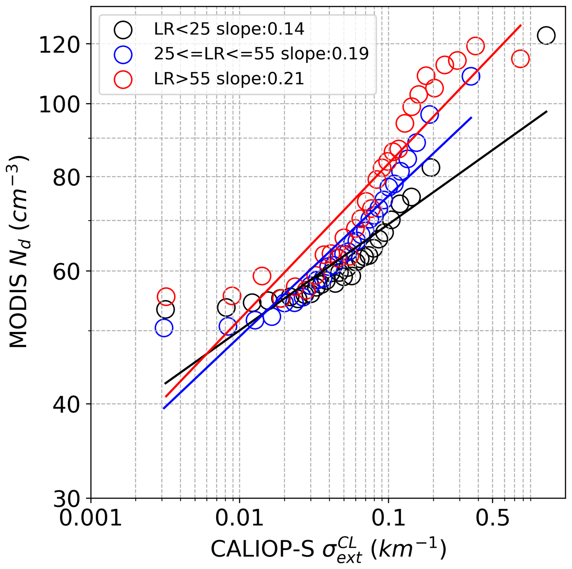
Figure 11 Binned relationship between N_d and ${\mathit{\sigma }}_{\text{ext}}^{\text{CL}}$ (ACI) for non-precipitating samples with 3 distinct values of aerosol lidar ratio (LR). LR<25 sr (black), LR within 25–55 sr (blue), and LR>55 sr (red).

The small values of precipitation/POP susceptibility should be interpreted as the lack of satellite data to show a significant influence of aerosols on the occurrence of precipitation. Being cognizant that the results could be dependent on the precipitation threshold applied in our study (−15 dBZ), we also repeated the precipitation susceptibility estimate using a more stringent definition by classifying precipitating samples as those with Z_max greater than −7 dBZ. The use of a higher precipitation threshold (not shown) did not qualitatively change the susceptibility variability of the map in Fig. 9a, yet the number of grids with statistically insignificant values substantially increased. Given the challenges of quantifying precipitation rate, especially for stratocumulus clouds, the use of airborne observations would be necessary to complement this satellite study with the use of precipitation rate retrievals, which will allow for more direct estimates of precipitation susceptibility.

Similar to Gryspeerdt et al. (2016), we explicitly partition the cloud adjustments into the N_d modulation of LWP and precipitation (POP), and the aerosol-cloud modulation of aerosols (${\mathit{\sigma }}_{\text{ext}}^{\text{CL}}$) on N_d. This method is more physically sound than directly calculating the effect of aerosol via aerosol-LWP and aerosol-precipitation regressions, because it takes into account the control variable (N_d) that mediates changes of aerosol in other cloud properties. Moreover, the partition applied here yields a more stringent condition for evaluating the significance of the cloud susceptibility as the requirement is that two regressions are required to produce meaningful values. Another rapid cloud adjustment commonly simulated by models and monitored with satellite observations is the lifetime effect, generally represented by changes in cloud (area) fraction as a function of aerosol concentration. This cloud fraction susceptibility is not reported in this study because cloud retrievals (N_d and LWP) are filtered using cloud fraction, with a threshold that directly affects the regression between CF and N_d. For example, Painemal et al. (2020) show a dramatic decrease in the CF–N_d slope when N_d values estimated in partially broken scenes are removed from the analysis. With optical retrieval biases sensitive to the type of cloud scene and sub-pixel scale cloud coverage, disentangling the physical signature from systematic biases in the CF–N_d relationship will make it difficult to determine the usability of such analysis using cloud observations from passive sensors.

5 Summary and final remarks

We computed aerosol-cloud interactions and cloud adjustments over the global ocean by combining aerosol retrievals from CALIOP-S, cloud properties from MODIS (CERES algorithm), and precipitation occurrence from CloudSat. This is the first global assessment, to the best of our knowledge, that relies on vertically-resolved aerosol retrievals that are vertically matched with the location of the cloud layer. Here we expand a previous study (Painemal et al., 2020) by considering most of the A-train record (2006–2017) and including the extratropical ocean. Moreover, we also incorporate estimates of liquid water path and precipitation susceptibilities due to aerosols to the analysis.

We corroborate that aerosol optical depth inadequately represents aerosols for the study of aerosol-cloud interactions in marine low clouds. More specifically, we found that AOD shows a negligible variation with cloud microphysics in the extra-tropics despite a strong correlation between cloud-layer aerosol extinction coefficient and N_d. We also found that the S-shape variations of N_d with AOD reported in numerous studies and reproduced here may not fully represent the physical processes governing cloud variability. This is because the S-shape is not replicated by the cloud-level aerosol extinction coefficient analysis presented here (Sect. 3.1) nor by airborne studies over the ocean. The limitation of using of AOD as an aerosol proxy for ACI is particularly manifested for values of AOD less than 0.1 and greater than 0.25, ranges for which N_d minimally varies with AOD. This finding indicates that the lack of sensitivity of N_d to AOD for typical aerosol loading over the ocean, is not indicative of the microphysical processes. We note that this conclusion is valid for the AOD magnitudes analyzed here, and it does not rule out other microphysical behaviors in more polluted conditions. Indeed, thermodynamically-driven saturation of N_d with aerosol loading over heavily polluted environments, especially over land, has been observed in several field studies (e.g. Ramanathan, et al., 2001). Lastly, it is important to emphasize that challenges in quantifying ACI goes beyond AOD. Indeed, near-surface aerosol retrievals weakly correlate with N_d and the associated linear regressions (Fig. S2) substantially differ from the analysis presented here (Fig. 4b), casting doubt on using near-surface ground-based aerosol observations for the quantifications of ACI and cloud adjustments.

The ACI metrics derived from combining CALIOP-S aerosol extinction coefficient, vertically collocated with the cloud layer, and MODIS products reveal regions with high sensitivity of clouds to changes in their N_d due to aerosols. These areas include the stratocumulus cloud regimes off the west coast of the continents, the Southern Ocean, and the extratropical Atlantic and Pacific Oceans in the Northern Hemisphere. High ACI values in stratocumulus cloud regimes are interpreted as the combined effect of a well-mixed boundary layer with readily available aerosols with a continental origin. However, it is somewhat surprising that the Southern Ocean, arguably the most pristine region on Earth, also witnesses high values of ACI, and relatively high N_d relative to other regions over the remote ocean with similar aerosol concentrations. This feature is possibly explained by enhanced aerosol activation driven by strong boundary layer turbulence in the Southern Ocean, especially in postfrontal conditions (e.g. Lang et al., 2021). In addition, abundant biogenic and sea-spray aerosols over the region (Humphries et al., 2021) can effectively serve as CCN.

In terms of LWP susceptibilities, this is negative in subtropical and extratropical regions, that is, LWP decreases with N_d. This decrease in LWP, also observed in other studies (e.g. Qiu et al., 2024), is generally interpreted as the drying effect of cloud top entrainment, which is enhanced with increasing N_d. In contrast, positive LWP-N_d slopes in the tropical ocean yield a modest LWP susceptibility because ACI is small and insignificant. This analysis also shows that the inverted-V shape in the LWP-N_d relationship is generally the consequence of spatial variability, which becomes more apparent when the calculation spatial domain is excessively large (Goren et al., 2025). Precipitation (POP) susceptibility, on the other hand, is also negative and consistent with the idea that aerosol suppresses precipitation. However, the magnitudes are only significant in narrow coastal areas in the eastern Pacific and southeast Atlantic. This is possibly related to the relatively small rain rates in these stratocumulus clouds, making them more susceptible to changes in their precipitation frequency than regions in the extratropics with more significant rain rates.

With the successful launch of the Earth Clouds, Aerosols and Radiation Explorer mission (EarthCARE; Wehr et al., 2023) in May 2024, the EarthCARE sensors will enable assessing aerosol-cloud interactions with products that will largely expand the capabilities of CALIPSO and CloudSat. For example, the improved sensitivity of the EarthCARE Cloud Profiling radar will enhance the detection of clouds relative to CloudSat, detecting clouds as low as 600 m. In addition, the EarthCARE Atmospheric Lidar (ATLID), being a high spectral resolution lidar, will provide direct observations of aerosol extinction coefficient and refined aerosol typing classification. Because of the sampling and collocation constraints in our study (which includes more than 11 years of A-Train observations), multiple years of EarthCARE observations will be required to replicate the statistical robustness of our analysis. Alternatively, efforts for expanding the lidar-cloud record through the homogenization of CloudSat, CALIPSO, and EarthCARE products will be necessary to corroborate and expand the findings of this study.