Long-term trace gas and black carbon measurements at the high-altitude station Mount Kenya: tropical atmospheric variability and the influence of African emissions

Long-term measurements of atmospheric composition are essential for understanding regional and global climate impacts. Although the Global Atmosphere Watch (GAW) programme provides a network of worldwide measurements, continuous atmospheric measurements across Africa remain scarce. This study presents multi-year in-situ measurements of trace gases and black carbon from the Mount Kenya GAW station (MKN) from 2020 to 2024, offering a unique dataset from equatorial Africa. Its location exposes MKN to contrasting air masses from both hemispheres, enabling detection of emissions and providing insights into tropical variability such as seasonal and diurnal cycles. We present carbon dioxide (CO₂), methane (CH₄), carbon monoxide (CO), ozone (O₃), and black carbon (BC) measurements and describe seasonal and diurnal variability. Atmospheric transport modelling combined with emissions estimates for CO and methane were used to distinguish African and non-African contributions to greenhouse gases and air pollution. CO and BC were mainly linked to household fuel use and industrial energy, with biomass burning contributing during dry seasons. Methane variability was driven by agriculture and seasonal wetlands, but large uncertainties remain in all emission estimates. We further compare the measurements from 2020–2024 with trace-gas data from 2002–2012. More positive trends were observed for CO₂ and CH₄ in agreement with global patterns, whereas O₃ exhibited non-significant positive trends in the recent period, consistent with findings from previous studies. CO trends were less conclusive due to the influence of sporadic biomass burning events, which complicate long-term trend detection. Comparison of the observations with Copernicus Atmospheric Monitoring Service (CAMS) model products shows CAMS fails to capture O₃ and BC dynamics during rainy seasons. Overall, our results demonstrate the value of MKN observations for evaluating atmospheric models and emission inventories, and underscore the urgent need to expand measurement infrastructure across Africa to improve understanding of atmospheric processes and climate impacts.

1 Introduction

The WMO Global Atmosphere Watch (GAW) Programme of the World Meteorological Organization (WMO) is an international framework dedicated to long-term, systematic and global observations of atmospheric composition (WMO, 2014). At the same time, GAW is complemented by several more specialized international networks that focus on particular species, techniques, or regions. Among these, the Network for the Detection of Atmospheric Composition Change (NDACC) (De Mazière et al., 2018), a contributing network to GAW, coordinates high-quality remote-sensing observations, and NDACC in turn includes affiliated cooperating networks such as AGAGE (Advanced Global Atmospheric Gases Experiment) (Western et al., 2025), SHADOZ (Southern Hemisphere Additional OZonesondes) (Thompson et al., 2025), and the NOAA Halocarbons and other Atmospheric Trace Species (HATS) program (Montzka et al., 1999). Together, these networks of hundreds of stations in total form an integrated global observing system that strengthens and broadens the capabilities of GAW. The observations deliver high-quality data from spatially representative sites that monitor atmospheric conditions, ideally with minimal local influence. This global framework is essential for understanding large-scale patterns and long-term trends in atmospheric composition. However, despite its wide reach, significant observational gaps remain – particularly across tropical regions and the Global South. Africa, though one of the most climate-vulnerable continents, is particularly under-represented in atmospheric monitoring networks, including for greenhouse gases (GHGs), primarily due to different national priorities, limited resources and infrastructure in emerging economies

Continuous GHG observations are essential for verifying and reducing uncertainties in bottom-up emission estimates, as demonstrated in Europe (Henne et al., 2016; Saboya et al., 2024) or other regions (Bukosa et al., 2025). Despite a few monitoring stations (e.g. Morgan et al., 2015; Labuschagne et al., 2018; Tiemoko et al., 2023), much of Africa still lacks the comprehensive GHG monitoring needed for robust emission assessments. This study explores the lessons learnt from the long-term data measured at the remote, high-altitude GAW station on Mount Kenya (0.062° S, 37.297° E, 3678 m a.s.l.). Besides an extensive data analysis to investigate atmospheric variability, we simulate air masses with an atmospheric transport model and combine them with emissions from bottom-up emission inventories. This integrated approach allows us to explore not only temporal variability but also the spatial and sectoral origins of the observed species. This assessment is made with full recognition that a denser GHG observation network across the continent is ultimately needed for robust verification and constraint of emission estimates.

The Mount Kenya station (MKN), operational since 1999, represents a unique monitoring site in tropical Africa. The recurrent meridional migration of the Intertropical Convergence Zone (ITCZ) that oscillates between approximately 20° N and 5–8° S depending on boreal and austral seasons (Henne et al., 2008a; Lashkari and Jafari, 2021; Hu et al., 2007), exposes the station to fundamentally different advection regimes throughout the year. These include continental air from the northeast during boreal winter and marine tropical air from the southeast in boreal summer. Moreover, more local anthropogenic processes and biomass burning emissions also influence the station, particularly during daytime. Based on early carbon monoxide (CO) and surface ozone (O₃) between 2002 and 2006, Henne et al. (2008b) showed that night-time observations reliably represent free-tropospheric background air. Using trajectory clustering, the authors identified six distinct regional flow regimes that drive the site's semi-annual CO cycle, including northern-hemisphere winter outflow and southern-hemisphere biomass-burning influence. Overall, the weak O₃ to CO correlations and rare pollution events demonstrated that Mt. Kenya provides a baseline perspective on tropical free-tropospheric composition, with interannual variability largely governed by southern African biomass-burning emissions. More recently a global tropospheric O₃ study included evaluation of east African O₃ trends for more than 20 years of Nairobi O₃ soundings. Total tropospheric O₃ changes (surface to tropopause) were estimated at approximately 1.5 % to 3.5 % per decade for the period of 2000 to 2023 (Thompson et al., 2025; Van Malderen et al., 2025) with the lower value representative of a trend at the altitude corresponding to Mt Kenya. Increases near the surface were closer to +5 % per decade because Nairobi is a polluted city of more than 4 million inhabitants.

The continuous and comprehensive greenhouse gas and air pollution datasets at MKN are unprecedented in the tropical African region and underline the importance of the MKN measurement site. While early carbon monoxide (CO) and surface ozone (O₃) data were reported previously (Henne et al., 2008b), the renewal of the power line has enabled largely gap-free, continuous aerosol measurements since 2015, and measurements of carbon dioxide (CO₂), methane (CH₄), CO, and surface O₃ since December 2019. Multiple trace gases were measured with flask samples at MKN by the Global Monitoring Lab (GML) of the National Oceanic and Atmospheric Administration (NOAA) from 2003 to 2011 (e.g. Lan et al., 2025), but were not continued afterwards. Kirago et al. (2023) investigated MKN CO in-situ and flask measurements up until 2022, but more recent years and other species have not yet been explored. Indeed, this study presents the first comprehensive analysis of the recent continuous datasets, focussing on the period 2020 to 2024.

Few studies have investigated similar compounds in the region. DeWitt et al. (2019) studied GHGs and air pollutants at the Rwanda Climate Observatory (Mt. Mugogo, 2590 m a.s.l) from 2015 to 2017. They demonstrated that their elevated site in equatorial East Africa was strongly influenced by both northern and southern hemispheric biomass-burning seasons, while also capturing substantial local combustion signatures. These findings highlight the importance of high-altitude stations for characterizing regional background air masses in Africa, a role similarly fulfilled by our Kenyan site. Earlier black carbon (BC) and aerosol measurements in East Africa have been analysed at urban and rural sites (Kirago et al., 2022; Gatari and Boman, 2003; Makokha et al., 2017; Khamala et al., 2018), but the recent multi-year BC data from MKN were not included. In addition to the continental East African site MKN, the Maïdo station (2155 m a.s.l) on Réunion Island (Callewaert et al., 2022) and the Lamto station (155 m a.s.l.) in Côte d'Ivoire (Tiemoko et al., 2021, 2023) provide tropical data on GHGs and air pollutants. Observations of CO₂, CH₄, and CO at Réunion Island showed that surface mole fractions are dominated by local influences (urban emissions at Saint-Denis, and biospheric fluxes at the high-altitude Maïdo station), whereas column measurements mainly reflect long-range transport from Africa, Madagascar, and distant biomass-burning regions. Because Lamto is a low-elevation site, multi-year observations showed that local wetland emissions, agricultural activities, and seasonal biomass burning, together with regional seasonal transport patterns, strongly shaped the variability of CO₂, CH₄, and CO in West Africa. The continuous, remote MKN measurements fill a critical gap in the tropical observation network.

In this study, we (i) analyse in-situ trace gas and aerosol measurements at MKN, (ii) evaluate the performance of Copernicus Atmospheric Monitoring Service (CAMS) model products for several species, (iii) compare surface ozone with vertical profiles from ozonesondes launched in Nairobi, (iv) simulate atmospheric transport using the particle dispersion model FLEXPART, and (v) combine transport simulations with bottom-up emission inventories for fires, wetlands, and anthropogenic sources.

This work was conducted within the Horizon Europe Coordination and Support Action “Knowledge and climate services from an African observation and Data research Infrastructure” (KADI), which aimed to strengthen Africa's climate knowledge base and provided a design for a pan-African atmospheric and climate observation system. The results presented in this study highlight the insights that can be gained from existing long-term measurements and underscore the urgent need to expand observational coverage across the African continent.

2 Data and Methods

2.1 The Mount Kenya station

The GAW Global station Mt. Kenya (MKN), located at 0.062° S, 37.297° E (WMO Integrated Global Observing System (WIGOS) Station Identifier (WSI) 0-20008-0-MKN), is situated on the north-western slope of Mt. Kenya at an altitude of 3678 m a.s.l. and is surrounded by alpine grassland and shrubs. As part of the Mt. Kenya National Park, the whole mountain area is protected and there are minimal local anthropogenic emissions, making the site suitable for continuous observations of the tropospheric background composition. Access by car is possible to the Old Moses Camp, located 300 m below and approximately 1.9 km northwest of the station. The closest settlement is situated 17 km in north-westerly direction, the closest city (Nanyuki) lies 27 km westwards at 1900 m a.s.l (Henne et al., 2008a).

MKN was established under the World Meteorological Organization (WMO)/United Nations Development Programme (UNDP)/Global Environment Facility (GEF) programme GLO/91/G32 in the mid-1990s and was officially inaugurated in October 1999. Due to limited power supply, it has operated on an irregular basis until 2014, when the power line was completely renewed. Nowadays, Mount Kenya is one of the very few high-altitude observatories in East-Africa (Alberti et al., 2023) and is among the best-equipped mountain stations in terms of atmospheric composition in the region.

The climate in Kenya is governed by the seasonally varying position of the ITCZ. The ITCZ lies North of MKN in boreal summer and south of MKN in boreal winter. The recurrent ITCZ displacement leads to different advection regimes in Equatorial Africa (see Fig. 2) with two rainy seasons from March to May (MAM) and October to December (OND), when the ITCZ crosses the equator (Nying'uro et al., 2024; Palmer et al., 2023; Lashkari and Jafari, 2021; Wainwright et al., 2019; Hart et al., 2019; Nicholson, 2018, 2017). The months in-between are characterized by a short dry season from January to February (JF) and a long dry season from June to August. September is a transitional month, with remaining dry conditions but higher temperature than in previous months. In this study, we count September as part of the long dry season (JJAS). Rainfall at MKN is governed by the mentioned rainy seasons, with maximum precipitation in April (see Fig. A1). However, precipitation measurements at MKN reveal larger values in August and September than expected from the regional seasonal classification (Fig. A1). This local precipitation is mainly governed by advection of Congo air masses (e.g. Hart et al., 2019), which converge around northern and western parts of MKN, leading to lifting air masses with showery precipitation. Nevertheless, we use the more regional classification of JJAS as “dry season” in our study. Daily minimum and maximum temperature at MKN vary on average between 4 and 11 °C. For more insights on the meteorological and climatological conditions and a comprehensive overview of the station characterization, refer to Henne et al. (2008a). Statistical data analysis of early carbon monoxide and ozone measurements (2002–2006) and air mass trajectory clustering confirmed the large-scale representativeness of the station and suitability of the location for background observations, specifically during the night (Henne et al., 2008b).

2.2 Observations

In-situ observations of greenhouse gases and air pollutants have been performed at the MKN station since the early 2000s, providing a unique long-term dataset for equatorial Africa. In 2006, issues with the station's power supply resulted in an interruption to the early CO and O₃ measurements. In 2008, there was an attempt to implement continuous GHG measurements, but it was unsuccessful due to severe damage to the power line caused by a wildfire in 2009. In 2010, the power supply was completely disconnected, but a new power line was installed in 2014, and continuous gas measurements were resumed in December 2019. In the following analysis, we therefore focus mainly on the continuous data from 2020 to 2024. The measurements are usually level 0 data stored as 1 min averages. Quality-controlled data are provided with 1-hourly temporal resolution.

For a better visualization and to obtain smooth seasonal cycles, we applied a curve fitting method provided by NOAA (https://gml.noaa.gov/ccgg/mbl/crvfit/crvfit.html, last access: 9 September 2025). The corresponding python code is publicly available (https://gml.noaa.gov/aftp/user/thoning/ccgcrv/, last access: 9 September 2025). The curve fitting method, also called CCGCRV (Carbon Cycle Group, Earth System Research Laboratory (CCG/ESRL), NOAA, USA), is a slight modification of the filtering approach presented by Thoning et al. (1989) and has been described and used in multiple studies (e.g. Pickers and Manning, 2015; Cristofanelli et al., 2024). The method first fits a 3rd order polynomial and 4th order harmonic function. Afterwards, the data is smoothed with a fast Fourier transform (FFT), and filtered with a low-pass filter, for which we use a short-term cut-off frequency of 80 d and a long-term cut-off of 667 d to remove remaining oscillations. To obtain the unbiased seasonal variability, any linear trend was removed.

2.2.1 In-situ CO₂, CH₄, CO, and O₃ measurements

Since December 2019, carbon dioxide (CO₂), methane (CH₄), and carbon monoxide (CO) observations have been performed with a commercially available Wavelength-Scanning Cavity Ringdown Spectrometer (Picarro Inc. G2401) coupled to a custom-built calibration unit. Ambient air is dried prior to analysis by means of a Nafion dryer (Permapure PD-50T-24SS). An experimentally determined correction function was applied to account for the interference of residual water vapour in the determination of dry air mole fractions. Measurements are calibrated about once a week with three reference gases, purchased from the GAW Central Calibration Laboratory at NOAA in Boulder, Colorado. A fourth reference gas is measured every second day to account for short-term sensitivity changes. In between these reference gas measurements, a fifth reference gas (target) is also measured every second day for quality control, i.e. it is treated as unknown in the same way as the ambient air data. The air inlet is approximately 10 m above ground. The air is drawn through $\mathrm{1}/\mathrm{4}$ in. outer diameter Synflex 1300 tubing with a flow rate of approximately 4 L min⁻¹ into the valve unit in the laboratory container. From there, the sample is directed through a $\mathrm{1}/\mathrm{4}$ in. outer diameter Synflex 1300 tubing, the Nafion dryer, and a sintered stainless steel filter of 7 µm pore size into the analyser. The Nafion dryer is connected in reflux mode, using the dry sample gas that is expelled from the analyser as counterflow gas of the dryer. A vacuum is applied to the counterflow to improve the drying efficiency. The residence time in the inlet is about 6 s.

Early CO measurements (2002 to 2006) were performed with a non-dispersive infrared (NDIR) analyser (Thermo Scientific TEI48C TL) as described in Henne et al. (2008b). The early CO data availability deteriorated in summer 2006 since the observations suffered from frequent power outages. The instrument was finally decommissioned during the power line replacement between 2010 and 2014.

Since the beginning of the surface ozone (O₃) observations in 2002, O₃ has been measured with in-situ instruments based on the UV absorption technique (Thermo Scientific, models 49 and 49C) as described in Henne et al. (2008b). Since September 2021, two UV absorption photometers, a Thermo 49C and 49i, have been operating in parallel. The air intake for the O₃ measurements is approximately 1.7 m above the roof of the container, and 4.5 m above ground. The inlet is made from glass tubing with an inner diameter of 5 cm, which also serves as a manifold. It is flushed at a high flow rate by a blower. The O₃ instruments are connected to the manifold with approximately 2 m of $\mathrm{1}/\mathrm{4}$ in. outer diameter perfluoroalkoxy (PFA) tubing. Polytetrafluoroethylene (PTFE) membrane filters with a pore size of 5 µm are installed upstream of the instruments to protect the instruments from particles. The total residence time is estimated to be less than 10 s.

2.2.2 Aerosol measurements

Aerosol measurements are performed in accordance with the GAW recommendations for aerosol sampling (WMO, 2016) and were implemented when the station was commissioned in 1999, and then renewed in March 2015. Data before 2015 are of unknown quality due to the frequent power outages and sparingly available. Since 2015, a custom-designed total suspended particulate matter (TSP) inlet is utilized as recommended for stations that are frequently in clouds. Given the site's dew point conditions and the availability of a temperature-controlled laboratory at the station, sampling is performed without additional drying. Periods during which the relative humidity (RH) exceeds 40 %, an occurrence normally associated with issues in the station's room temperature control system, are flagged appropriately.

The equivalent Black Carbon (BC, hereafter) mass concentrations reported in this study were derived from two aethalometer instruments (Magee Scientific Models AE31 (March 2015–July 2024) and AE33 (January 2024–to date)) with time resolutions of 5 and 1 min, respectively. The raw data processing adhered to the current GAW/ACTRIS recommendations (WMO, 2016; Zanatta et al., 2016). In a first step, the light absorption coefficient was calculated from the 880 nm wavelength channel of both instruments. This included compensation for non-linear filter loading effects as well as correction for multi-scattering effects in the AE31 instrument (Weingartner et al., 2003). The multi-scattering correction was achieved using a constant C-value of 3.5 (Zotter et al., 2017) in the absence of simultaneous measurements using an absorption reference method in accordance with the GAW recommendations (WMO, 2016). Data from the AE33 instrument were processed following the ACTRIS guidelines (Müller and Fiebig, 2021) using a harmonization factor of 1.76 in combination with an instrument internal M8060 filter tape factor of 1.39. In a final step, the derived light absorption coefficients of both instruments were converted to equivalent BC concentrations using a constant mass absorption cross-section (MAC)-value of 7.24 m² g⁻¹ (Zanatta et al., 2016). With this processing scheme, the BC data of the two instruments showed a very good agreement (R²=0.97) in their one-year overlapping period in 2023. The AE33 instrument showed on average 10 % higher BC concentrations in comparison to the AE31 instrument (Fig. B1).

2.2.3 Ozonesonde measurements

ENSI ECC ozonesondes have been launched from the Kenya Meteorological Department (KMD) Headquarters at Dagoretti Corner in Nairobi (https://oscar.wmo.int/surface/#/search/station/stationReportDetails/0-20008-0-NRB, last access: 12 May 2026) on Wednesdays on a weekly basis since 1996. These soundings contribute to both, the WMO Global Atmosphere Watch GAW program (https://woudc.org/en/data/, last access: 25 August 2025) and the NASA SHADOZ program (https://tropo.gsfc.nasa.gov/shadoz/Nairobi.html, last access: 25 August 2025). For the analysis presented here, ozone mole fraction time series were extracted from the profile data (SHADOZ v6 data) at 700 hPa for comparison with the in-situ surface ozone measurements, which is the level that correlated best with CAMS data (see Sect. 2.3).

2.3 Atmospheric modelling data

Due to the sparse availability of continuous measurements in the tropical region, the MKN measurements are highly valuable for validation of atmospheric models. We compared the MKN measurements with model data from CAMS (CAMS, 2025). For comparison of the model output with the MKN measurements, we selected for each species the CAMS grid for which CAMS data correlates best with the corresponding measurements over the entire time period. In the following, we describe the CAMS products used in our analyses.

2.3.1 CO, O₃ and black carbon data from CAMS reanalysis

For direct model comparison with CO, O₃ and BC measurements at Mt. Kenya, we used EAC4 (ECMWF Atmospheric Composition Reanalysis 4) global reanalysis data in the region between 0.7° N to 0.8° S and 36.5 to 39 ° E and at pressure levels from 1000 to 600 hPa (CAMS, 2020b, last update: 19 June 2025). The data have a temporal resolution of 3 h and a spatial resolution of 0.75 °. For direct comparison with MKN measurements, we chose CAMS data at 700 hPa, the level which correlates best with our CO and CH₄ measurements. For CAMS black carbon data, we used the sum of hydrophilic and hydrophobic black carbon mass mixing ratio (kg kg⁻¹). To convert it to mass concentrations (µg m⁻³), we scaled it with the air density, calculated from the temperature given by CAMS for that level and grid cell and a fixed pressure of 700 hPa.

2.3.2 CO₂ and CH₄ data from CAMS invGG

CO₂ and CH₄ measurements were compared with data from the CAMS global inversion-optimised greenhouse gas fluxes and concentrations (invGG) dataset (CAMS, 2020a). For CO₂, we downloaded model outputs that used satellite observations as input-data (CAMS, 2020a, last update: 20 June 2025). Before July 2023, the spatial resolution was 2.5 ° lon × 1.27 °lat, afterwards it increased to 1.4 ° lon × 0.7 ° lat. The temporal resolution is 3 h. For comparison with MKN measurements, we selected the CAMS grid with highest correlation with our measurements for the first period (until July 2023), which corresponds on average to 658 hPa in that period (model level 26).

The CH₄ invGG data uses surface air-samples and satellites as input (CAMS, 2020a, last update: 9 May 2025). The assimilated surface observations are ground-based observations from the NOAA network (Segers and Nanni, 2023). The product is thus independent from our MKN measurements. The spatial resolution for the CH₄ invGG product is 2 ° lat × 3 ° lon before 2022 and 1 ° × 1 ° afterwards, the temporal resolution is 6 h. The CAMS grid selected for MKN comparison, with highest correlations to measurements for the first period (until 2022), was on model level 9, which corresponds on average to 614 hPa.

2.4 Atmospheric transport model and emission data

To understand the origin and variability of trace gases and aerosols observed at MKN, it is essential to consider the influence of large-scale atmospheric transport and regional emission sources. The station's central location in equatorial Africa exposes it to contrasting air mass regimes from both hemispheres, resulting in a complex mixture of natural and anthropogenic signals. While in-situ measurements offer high-resolution temporal data, they do not provide direct information about the geographic or sectoral origin of the observed compounds. To address this, we use the Lagrangian particle dispersion model FLEXPART to simulate air mass transport to MKN. These simulations yield residence time distributions that describe the sensitivity of the station to air coming from different regions. By folding these residence times with spatially resolved emission inventories, we derive quantitative source contribution estimates to the measured concentrations. This approach enables us to disentangle the influence of biomass burning, wetland activity, and anthropogenic processes. Although the results depend on the transport simulations and cannot be used for quantitative verification of the emission inventories, they offer valuable insights into the processes driving variability at MKN and allow for a broad evaluation of the quality of current emission inventories for the African continent.

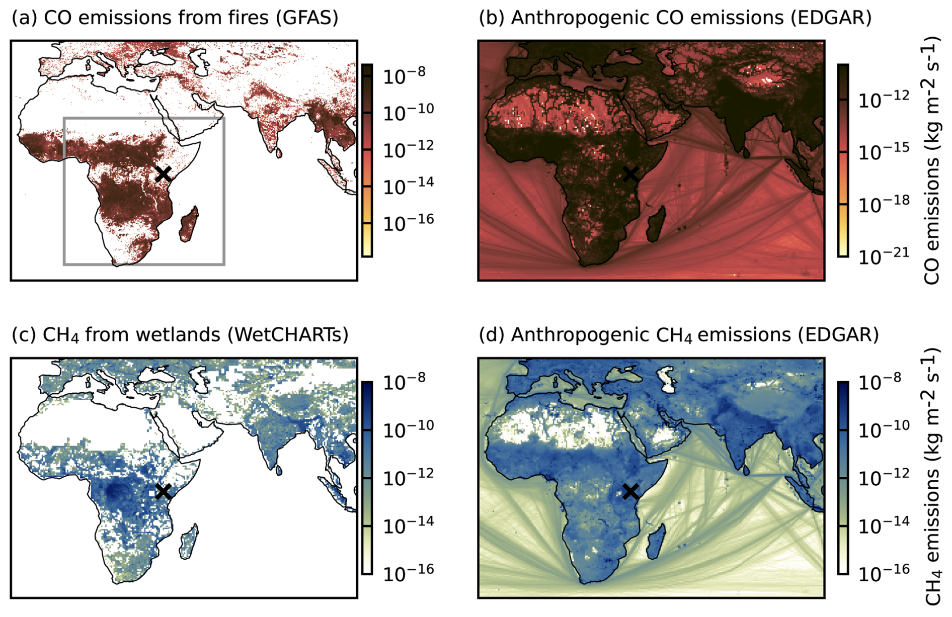
Figure 1 Spatial distribution of CO emissions from fires (a) and anthropogenic processes (b), and CH₄ emissions from wetlands (c) and anthropogenic processes (d) used for folding with FLEXPART, averaged for the year 2020. The grey box in panel (a) represents the nested domain (Sub-Saharan Africa) used in this study. The location of MKN is marked with a cross. Data are retrieved from GFAS, WetCHARTs and EDGAR, see text for details.

As emission inventories, we used satellite-based fire emissions from the CAMS Global Fire Assimilation System (GFAS), wetland methane emissions from WetCHARTs (Bloom et al., 2024), and anthropogenic emissions from the Emissions Database for Global Atmospheric Research (EDGAR) (Crippa et al., 2024b). We concentrate on the regional emissions where sensitivities and emissions are largest and include emissions from most of Sub-Saharan Africa (0° W to 60° E and 20° N to 35° S, see Fig. 1a). The global WetCHARTs and EDGAR emission data were handled and prepared to fit our study area using the Python package emiproc (Constantin et al., 2025). Averaged maps for CO and CH₄ emissions in 2020 from those datasets are shown in Fig. 1.

2.4.1 Particle dispersion model FLEXPART

FLEXPART is a Lagrangian particle dispersion model that is widely used to trace atmospheric transport from the global to the regional scale (Stohl et al., 2005; Bakels et al., 2024). In this study, we apply it in time-reversed backward mode to characterize the pathways of air masses arriving at MKN. Additionally, the model provides quantitative source sensitivities that can be folded with surface mass fluxes (emissions) to obtain tracer concentrations at the release location (here, MKN), representing regional concentration contributions.

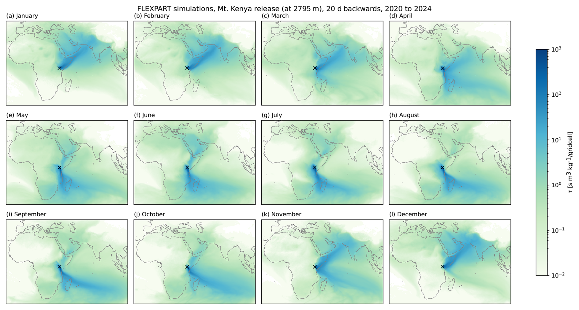
Figure 2 Monthly averaged FLEXPART footprints (2020–2024), showing the averaged residence time τ of air from backward simulations released at Mt. Kenya. The location of MKN is marked with a cross.

FLEXPART was driven with input meteorology taken from the European Centre for Medium Range Weather Forecast (ECMWF) operational high-resolution (HRES) forecast/analysis. These fields were available with a spatial resolution of 0.5° × 0.5° every 3 h. 50 000 particles were continuously released for each three-hour observation period at MKN and traced back to their origin 20 d earlier or until they crossed the border of the output domain. We performed simulations over two spatial domains: one covering most of Sub-Saharan Africa (0° W to 60° E and 20° N to 35° S, see Fig. 1a) with 0.1 ° resolution, and a second, larger domain covering the entire African continent and the adjacent Indian Ocean region (20° W to 110° E and 50° N to 40° S, see Fig. 2) with 0.5 ° resolution to obtain a larger overview of overall dynamics. The model particles were treated as inert compounds, hence no chemical transformation nor deposition was considered.

Due to the limited horizontal model resolution and the topography, the FLEXPART model altitude at MKN (2272 m) does not correspond to the true station altitude (3678 m). Therefore, we used a FLEXPART release height of 2975 m, which is the centre between the model altitude and the station altitude, as suggested by Brunner et al. (2012) and Henne et al. (2016).

To determine the background levels of CO, CH₄ and BC, we combined the FLEXPART simulations with CAMS concentration fields at the end points of FLEXPART model particles. CAMS concentrations were interpolated in space and time to particle positions and averaged over all particles released at a given time interval, representing the background concentration. For that, we used the same CAMS data as described above, but extended them to the large domain covering Africa and the Indian Ocean region. For the CH₄ background, we used CAMS data with surface observations only assimilated in the model, whereas for direct measurement comparison of CH₄, the satellite and surface data were assimilated in the product used, as described in Sect. 2.3.2. FLEXPART simulations could only be computed until the end of 2023. Therefore, the FLEXPART-related analyses in Sect. 3.3 are limited until the end of 2023. Furthermore, FLEXPART simulations are missing in October 2023 due to some technical issues.

2.4.2 CO, BC and CH₄ emissions from fires (GFAS)

Data from the CAMS Global Fire Assimilation System (GFAS) were used to investigate CO, BC and CH₄ emissions from fires (CAMS, 2022, last update: 20 January 2025). The data relies on satellite observations from NASA Terra MODIS and Aqua MODIS fire products. Emissions of various species are estimated based on given emission factors for each species (Kaiser et al., 2012). We use daily CO, BC and CH₄ data with a spatial resolution of 0.1 ° lat × 0.1 ° lon.

2.4.3 Wetland emissions (WetCHARTs)

The WetCHARTs dataset provides estimates of global wetland CH₄ emissions based on multiple terrestrial biosphere models (Bloom et al., 2017). We use WetCHARTs monthly data (v1.3.3) for 2020 to 2021 with a 0.5 ° × 0.5 ° spatial resolution (Bloom et al., 2024, last update: 3 March 2025) and average the output of 18 ensemble models. The processed FLEXPART output (sum of all trajectory days) is then folded with a constant emission inventory for each month. For the years 2022 and 2023, we used monthly averages from the last fully available year (2021).

2.4.4 Anthropogenic emissions (EDGAR)

For anthropogenic emissions, we use annual sector-specific grid maps from the Emissions Database for Global Atmospheric Research (EDGAR), v8.1 for CO and BC (EDGAR v8.1, 2025) and “EDGAR_2024_GHG” for CH₄ (EDGAR, 2025) with a spatial resolution of 0.1 ° lat × 0.1 ° lon. Details about the methodology of the EDGAR inventories as well as sectorial contributions in different regions can be found in Janssens-Maenhout et al. (2019), Crippa et al. (2024b), and Crippa et al. (2024a).

The emission inventories are based on statistics and assumptions about human behaviour and regional distribution, and uncertainties are large. For methane, Janssens-Maenhout et al. (2019) reported an uncertainty of 60 % for non-Annex1-countries, which includes the whole African continent. Uncertainties about emissions of air pollutants (in our case, CO and BC) in Africa are difficult to provide (Monica Crippa, personal communication, 2025). Certain sectors related to particulate matter emissions, combustion of biofuels in residential sectors and waste management may have particularly large uncertainties. The BC emission inventories are generally lower grade for domestic than for open burning, because activity and emission factors are largely unknown and highly variable (Bond et al., 2013). For example, Kerosene lamps can have 20 times higher BC emissions factors than the ones currently represented in inventories (Lam et al., 2012). Furthermore, certain countries provide less robust statistics than others.

We grouped the given emission categories in the EDGAR inventories into five overall sectors:

• i.

  industry, including the sectors “oil refineries and transformation industry” and “combustion for manufacturing”,

• ii.

  transportation (only for CO and BC), including “shipping” and “road transportation”,

• iii.

  waste (only for CH₄), including “waste water handling” and “solid waste landfills”

• iv.

  agriculture (only for CH₄), including “agricultural soils”, “agricultural waste burning”, “manure management”, and “enteric fermentation”, and

• v.

  energy, including “fuel exploitation” (only for CH₄), and “energy for buildings”, which includes households and commercial activities, such as solid fuel burning for domestic energy production.

EDGAR emission inventories were available until 2023 for CH₄ and until 2022 for CO and BC, afterwards we used the inventory of the last available year. To avoid double counting, we removed agriculture emissions from the CO and BC inventory, because those emissions (mostly due to agriculture-related fires) are mostly already accounted for in the GFAS fire emissions.

2.4.5 Emission source sensitivities

To obtain the sensitivities of emission sources at the MKN station, the residence times simulated with FLEXPART were combined with the emission data. For this, FLEXPART residence times τ in a 0.1° × 0.1° grid box (given in s m³ kg⁻¹ per grid cell) were multiplied with the fluxes from the emission data (in kg m⁻² s⁻¹) and summed up afterwards spatially to obtain a single contribution at MKN per day. The FLEXPART sampling height was set to 50 m above ground, and the volume of the grid cells and the molar weights of the gases were considered as described by Henne et al. (2016). Black carbon emissions were scaled with an approximated air density for dry air of 1.1839 kg m⁻³ (at 25 °C and 1013 hPa) for each grid cell volume. A constant emission map was applied to each FLEXPART footprint (sum of all trajectory days) for each year (EDGAR) or each month (WetCHARTs). For GFAS, however, we used daily averaged fluxes for each day of the trajectory.

3 Results and Discussion

3.1 Seasonal influences of air masses

Using the FLEXPART model, we simulated 3-hourly footprints for artificial particle releases at MKN for the whole study period (2020–2024). The residence time τ averaged for each month is shown in Fig. 2. The simulations confirm the dominant role of the ITCZ, which acts as a dynamic boundary that creates seasonally distinct hemispheric atmospheric regimes at MKN (Henne et al., 2008b). MKN is predominantly exposed to north-easterly advection from December to March, and to south-easterly advection from July to October, with the remaining months indicating the transition periods (Fig. 2). The atmospheric transport simulations indicate that processes above Western Africa only have an indirect impact on the observations at MKN.

3.2 Time series and trend analyses

Continuous GHG measurements at MKN have become available since 2020, as detailed in Sect. 2.2, while earlier in-situ and flask measurements had been measured intermittently since 2002 (Fig. C1). Trends for different periods as distinguished by different colours in Fig. C1 are listed in Table C1. Monthly aggregates of both the continuous measurements and the flask analyses were used for the determination of trends by linear regression. The CO₂ trend intensified over the 23-year record. While flask measurements for 2002–2011 indicated an increase of less than 2 ppm yr⁻¹, recent observations show a rise of nearly 2.4 ppm yr⁻¹. This rate is consistent with global increases reported by the NOAA network (NOAA, 2025) but is slightly below the most recent decadal global growth rate documented by WMO (WMO, 2025). CH₄ trends during 2002–2011 were characterized by the temporary global near-steady state in atmospheric CH₄, before growth resumed in 2007 (Rigby et al., 2008). As a result, the early-period trend is comparatively weak, while recent observations show a significant increase of more than 12 ppb yr⁻¹, even exceeding the global mean growth rate of 10.6 ppb yr⁻¹ over the past decade (WMO, 2025). This acceleration aligns with recent assessments that the tropics dominate the latitudinal contribution of global CH₄ emissions (Saunois et al., 2025) and highlight Central Africa and tropical South America as the dominant contributors to the current net CH₄ flux to the atmosphere (Niwa et al., 2025).

The combined O₃ time series for 2002–2024 is the most internally consistent among the four trace gases discussed here, as it is based on continuous in-situ measurements using the same technique throughout. A statistically significant positive trend is found for the full period (2002–2024) of 0.20 ± 0.07 ppb yr⁻¹. Comparison of sub-periods indicates a slowdown in the ozone growth rate, with a stronger increase during the early years (2002–2006: 0.42 ± 0.88 ppb yr⁻¹) and a smaller trend in the more recent period (2015–2024: 0.14 ± 0.21 ppb yr⁻¹) though both not statistically significant. This behaviour is consistent with SHADOZ observations showing that free-tropospheric and total tropospheric ozone above Nairobi exhibit weak, statistically insignificant long-term trends over 2000–2022 of 0.05 to 0.08 ppb yr⁻¹ depending on the trend calculation approach (Van Malderen et al., 2025), with earlier positive tendencies levelling off in recent years (Thompson et al., 2025). Our results also complement the conclusions of Cooper et al. (2020), who analysed long-term ozone trends from 27 remote ground-based sites worldwide but could not include East African stations owing to the lack of sustained observations at the time. While highlighting the African region as a major observational gap, they concluded that, globally, free-tropospheric ozone has increased since the mid-1990s, in contrast to Europe and North America, where surface ozone trends have largely flattened or declined since around 2000.

The long-term CO trend is the most difficult to interpret because it combines several measurement techniques, including in-situ NDIR and CRDS observations, different calibration strategies, and a mixture of in-situ, flask, and later again in-situ data. In addition, CO observations in the tropics are strongly influenced by biomass-burning emissions and by the varying strength of El Niño and La Niña events. These factors produce temporary CO enhancements, resulting in large interannual variability that often dominates any long-term trend signal. For the period 2002–2012, the CO trend derived from flask measurements is negative (−0.48 ± 1.28 ppb yr⁻¹), consistent with overall patterns observed at remote background sites (Patel et al., 2024). However, Patel et al. (2024) also highlight that trends in the tropics are less consistent than at higher latitudes because of the strong influence of biomass burning and climate variability. In contrast, the most recent period (2020–2024) shows a slightly positive trend, similar to that obtained for the full dataset. Depending on whether the early continuous measurements or the flask data are used, the overall CO trend ranges between 0.11 ± 0.33 and 0.63 ± 0.29 ppb yr⁻¹. These differences are likely related to the varying sensitivity of continuous versus intermittent flask sampling to episodic fire emissions. The long data gap from 2012 to 2019 also compromises robust trend determination.

Earlier conclusions from Mount Kenya CO and O₃ data (Kirago et al., 2023) determined a slightly positive trend for MKN CO data from 2002 to 2022. Furthermore, we observe that the seasonality does not differ substantially between previous and recent measurement periods (Fig. C1e–h). However, the February-maxima in CO₂ (Fig. C1e) and CO measurements (Fig. C1h) were larger in the 2002–2006 period (red and yellow lines) than in the recent period (blue line). Indeed, while Henne et al. (2008b), based on MKN measurements from June 2002 to June 2006, and DeWitt et al. (2019), using data from Mt. Mugogo (Rwanda) from 2015 to 2017, reported peak CO values in February, our more recent observations (2020 to 2024) show a shift, with maximum CO levels in July (Fig. C1h).

Larger and slightly earlier CO peaks in recent dry seasons (June/July 2020 to 2022) were also observed by Kirago et al. (2023), who investigated MKN CO measurements from 2002 to 2006 and 2020 to 2022. This shift in maximum CO values from February to July might be linked to seasonal changes in wildfire intensity, but it may also result from dynamical atmospheric changes. Further investigations would be needed to confirm those possibilities.

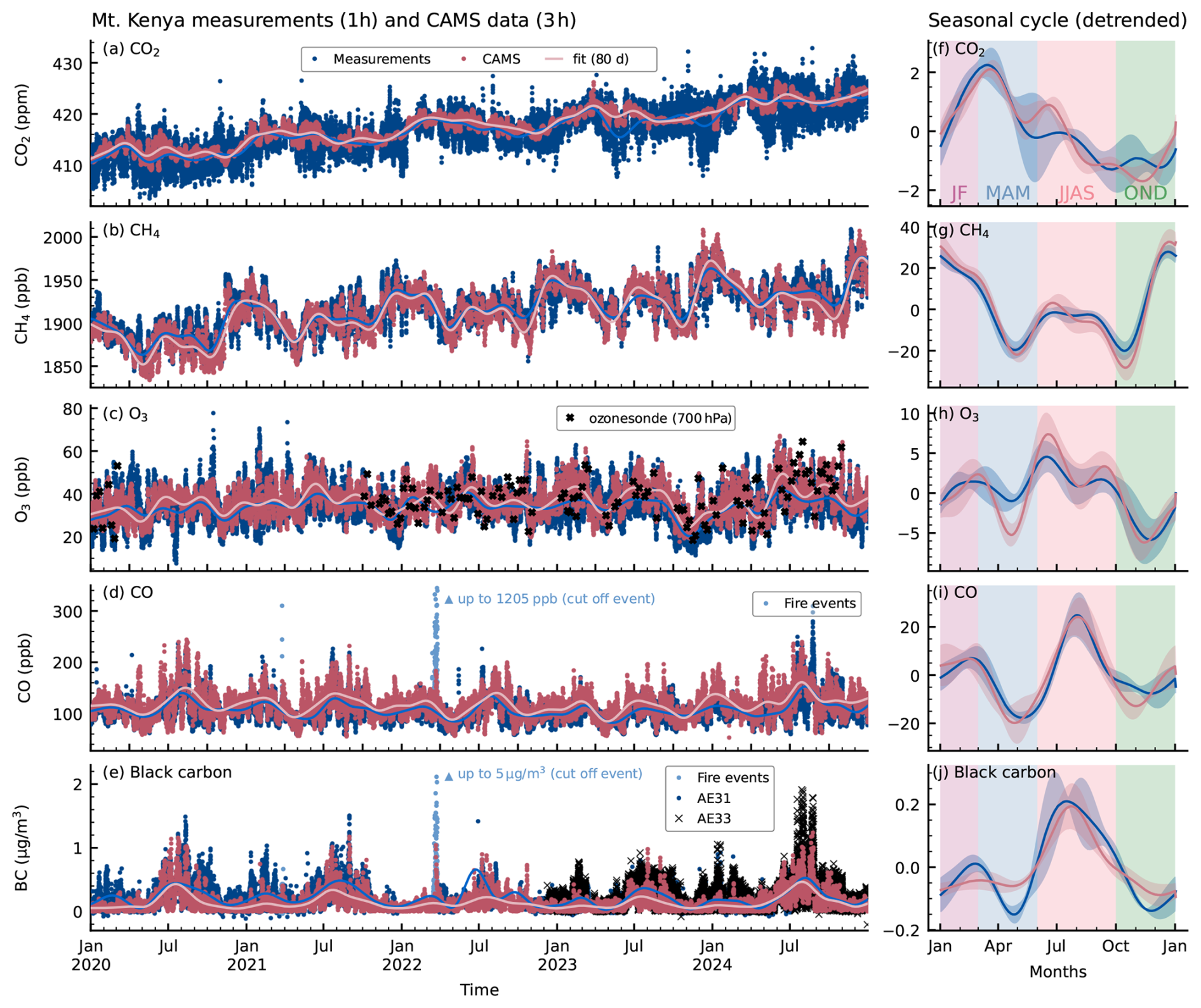
Figure 3 Measurements of CO₂, CH₄, O₃, CO and black carbon since 2020 and their seasonal cycles, compared to CAMS products (a–e). The dots show hourly (measurements) or 3-to-6-hourly (CAMS model) data points, the lines show the NOAA-fit using an 80 d filter. The right panels (f–j) show the corresponding detrended seasonal cycles based on the NOAA-fits. The shaded areas show the standard deviation over the 5-year period for each day of the year. The vertical shadings indicate the dry seasons (January–February (JF) and June–July–August–September (JJAS)) and wet seasons (March–April–May (MAM) and October–November–December (OND)).

The temporal evolution from 2020 to 2024 and the seasonal cycles for the five analysed species at Mt. Kenya are shown in Fig. 3, both for in-situ measurements and CAMS model data. Generally, we observe a good agreement between measurements and CAMS data, suggesting that the measurements are highly valuable for model validation in this region. The general larger variability in the measurements is partly due to their hourly resolution, whereas CAMS data shows 3-hourly values (or 6-hourly for CH₄), but mainly because the model misses some local variability.

The CO₂ CAMS data (Fig. 3a) have an even smaller variability than the other species. We observed that CAMS invGG generally only shows clear diurnal variations (> 1 ppm) up to approximately 850 hPa. At higher altitudes (lower pressure), the diurnal variability in the invGG product decreases and becomes negligible. At the selected CAMS level, the diurnal amplitude is on average only 0.04 ppm, which is a factor of 100 smaller than expected from measurements (see Sect. 3.2.2). These results suggest that despite the overall good agreement of the CAMS invGG CO₂ product with MKN measurements, the CAMS model is unable to resolve the diurnal cycle at the given altitude. We suspect the reason for this discrepancy is due to poor representation of the boundary layer in the CAMS model. Also for CH₄, the CAMS model at the selected level underestimates the diurnal cycle by a factor of 4 to 10 (depending on the season), but the underestimation is less pronounced than for CO₂.

CAMS O₃ data agree well with measurements (Fig. 3c). In addition to in-situ and CAMS O₃ data, we show ozonesonde measurements from the nearby launches in Nairobi. For each sounding profile, we chose measurements at a fixed pressure level (700 hPa) to compare with the in-situ measurements at MKN. Generally, the ozonesonde measurements agree well with the in-situ measurements. However, ozonesondes seem to report slightly higher values in 2024, which requires further investigation.

In 2023, the ozone in-situ measurements show smaller values than in other years, with a decrease starting approximately in September 2023 (Fig. 3d). This ozone decrease, which is also observed in ozonesonde measurements and in CAMS data, might be related to the El Niño event in 2023/2024 (Peng et al., 2024). Earlier El Niño events occurred in 2002/2003, 2009/2010, 2014/2015, 2018/2019 (https://ds.data.jma.go.jp/tcc/tcc/products/elnino/ensoevents.html, last access: 7 July 2025). In line with this hypothesis, previous ozone measurements (Fig. C1d) show decreased values towards the end of the years 2003, 2015 and 2019 (though less pronounced in 2019), which corresponds to the autumn/early winter following those El Niño events. Unfortunately, no measurements were available during the other El Niño events and further analyses would be required to better understand the underlying dynamical processes.

In the CO and BC time series, we observe that a nearby wildfire event in March 2022 led to a strong peak of up to 1205 ppb and 5 µg m⁻³, respectively. To avoid distortion of the figure, we cut the scale of the axis in Fig. 3d, e. Figure 3e shows BC measurements from two different instruments (AE31 and AE33). CAMS CO data agree well with CO measurements, whereas the agreement is slightly worse for BC, especially in 2024. In June/July 2024, CO and BC show increased values that are not reproduced by CAMS. We could not identify a single dominant local wildfire event in that period, but wildfire activity from July to September that was not detected by CAMS could possibly explain the differences.

3.2.1 Seasonality

The seasonal cycles show a common feature for CH₄, O₃, CO and black carbon (Fig. 3g–j) with two minima in April/May and November. This pattern can be explained by the seasonal variation of air masses and the displacement of the ITCZ (see Sect. 2.1), which has important implications for atmospheric composition measurements. The CO₂ cycles behave differently due to the strong seasonality of the sink, which features a different pattern.

The first minimum in April/May corresponds to the end of the long rainy season, when the ITCZ moves northward across Kenya, bringing clean air from the Indian Ocean (Fig. 2). This air mass is characterized by low amount fractions of CH₄ and CO, and low BC concentrations (Henne et al., 2008b). Despite this advection of clean air, ozone levels at MKN remain moderate during this period of the year (Fig. 3h), consistent with previous results by Henne et al. (2008b). Interestingly, CAMS fails to reproduce these moderate O₃ values in April, suggesting that the model may miss some ozone formation processes occurring during the transport in the rainy season. Another possibility is that CAMS underestimates vertical mixing during the ITCZ crossing. To investigate this seasonal underestimation, further analyses are needed, such as comparing CAMS ozone profiles with ozonesonde profiles.

A second minimum occurs in November, when the ITCZ shifts southward over Kenya, again resulting in dominant advection from the Indian Ocean (Fig. 2). CAMS overestimates BC concentrations during both April and November minima. This discrepancy could be attributed to a site- and potentially region-specific under-representation of BC scavenging and associated wet deposition processes in the model. It is known that deposition heavily depends on underlying aerosol particle size distributions, mixing state and precipitation intensity, etc., which are related to transport but also local site specific aspects (Ogren and Charlson, 1983; Bond et al., 2013; Vignati et al., 2010).

The annual maximum of CO and BC occurs during the dry season in July/August, which corresponds to the biomass burning season in the Southern Hemisphere. Ozone peaks earlier, in June, and again in September. These peaks are likely driven indirectly by biomass burning, which affects tropospheric O₃ through emissions of volatile organic compounds (VOCs) and nitrogen oxides (NO_x; DeWitt et al., 2019). The timing of O₃ maxima are not directly correlated with the CO and BC peaks, which may be explained by the complex tropospheric O₃ chemistry. Tropospheric ozone formation depends on the availability of VOCs, NO_x, and solar radiation, and is therefore not linearly related to emissions.

Unlike CO, BC and O₃, which all peak during the long dry season (JJAS), CH₄ amount fractions reach their maximum in December/January. During this time, northern continental air masses dominate MKN (Fig. 2). This correspondence suggests that CH₄ amount fractions at MKN are primarily influenced by northern continental air masses and associated emissions (in December/January), whereas highest levels of O₃, CO and black carbon originate from Southern Hemisphere biomass burning emissions (in July/August).

In contrast to the other species, CO₂ does not follow the same seasonal pattern (Fig. 3f). CO₂ values peak in March, and decline until November, before increasing again in early December. The lowest values occur between September and November, which mostly corresponds to the short rain period. This seasonal behaviour likely results from a combination of atmospheric transport and vegetation dynamics. Compared to the other species, CO₂ is strongly affected by vegetation activity, in addition to dynamical and anthropogenic influences. The pronounced increase in CO₂ starting in December and continuing through the dry months of January and February, reaching a maximum in March, is most likely driven by reduced photosynthetic uptake and increased plant respiration. During the long rains (March to June) the peak vegetation productivity leads to CO₂ uptake and decreasing CO₂ amount fractions. In the subsequent dry season, CO₂ briefly increases again in July, but decreases afterwards. This is surprising, as reduced vegetation activity during dry periods would typically lead to more respiration and hence higher CO₂ levels. However, air masses during this time predominantly originate from the southern Indian Ocean (Fig. 2), which suggests that vegetation is not the dominating factor. During the short rains from October to December, CO₂ remains rather constant, with a slight increase in November. This is again unexpected, as enhanced vegetation activity during rainy periods should reduce CO₂ levels. This is probably again related to changing air mass origins: in October, MKN receives air from the southern Indian Ocean, with increasing influence from the northern Indian Ocean and the Arabian Peninsula in November and December. These dynamical factors appear to outweigh local photosynthetic uptake during the rainy season. Finally, the CAMS CO₂ seasonality agrees well with the observations, but CAMS overestimates CO₂ in May and June (end of long rains) and underestimates CO₂ in November (short rains).

3.2.2 Diurnal cycles

The diurnal variability of all measured species and temperature at MKN is shown in Fig. 4. All species exhibit pronounced diurnal variability, with important differences during day and night. This variability is largely driven by meteorological mountain dynamics, as described by Henne et al. (2008a), who observed the development of thermally induced winds at Mt. Kenya, characterized by upslope winds during the day and downslope winds at night. This leads to transport of planetary boundary layer (PBL) air towards MKN during daytime. Henne et al. (2008b) concluded, based on detailed analyses of meteorological, CO and O₃ measurements, that MKN measurements represent free tropospheric conditions only at night (21:00–04:00 UTC, 00:00–07:00 local time), and a mixture of boundary layer and free tropospheric air during the day.

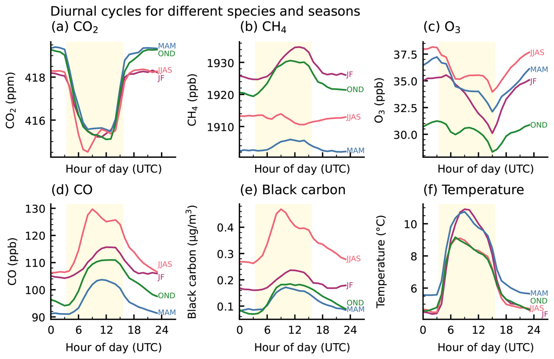
Figure 4 Diurnal cycles of measurements at Mt. Kenya for five measured species (a–e) as well as temperature (f) for dry seasons (January–February (JF, purple line) and June–September (JJAS, red line)) and wet seasons (March–May (MAM, blue line) and October–December (OND, green line)). The shaded area indicates the average daytime (from sunrise to sunset). All figures show the averaged diurnal cycle for 2020 to 2024, except for temperature, for which we use only data from 2022 to 2024.

The measurements are generally in line with the expected dynamical mechanisms. Nighttime CO₂ values drop rapidly by approximately 3 to 4 ppm after sunrise (Fig. 4a) with larger decreases typically observed during the wet season. These daytime reductions reflect lower CO₂ levels in the PBL driven by ecosystem uptake. Similar daytime CO₂ reductions have been observed at the high-altitude station Maïdo on Réunion Island in the southern Indian Ocean (Callewaert et al., 2022), where diurnal variability is primarily driven by surrounding vegetation uptake during the day and respiration at night. The 4 ppm nighttime decrease at MKN is also comparable to the boreal summer decline observed at the high-altitude station Mt. Cimone (5 ppm) in Italy (Cristofanelli et al., 2024). In contrast, lower-altitude African sites report substantially larger diurnal amplitudes, such as Saint-Denis on Réunion Island (∼ 10 ppm; Callewaert et al., 2022) and Lamto in Côte d'Ivoire (∼ 38 ppm; Tiemoko et al., 2021). These larger variations are likely due to higher absolute CO₂ amount fractions and more intense biospheric activity at lower elevations.

While CO₂ shows consistent diurnal patterns across all seasons, CH₄ is the only species that shows clear seasonal differences (Fig. 4b). From October to February, CH₄ amount fractions increase during the day, with peak enhancements of around 10 ppb in the afternoon. This period also shows the strongest diurnal variability, coinciding with the dominance of northern air masses. In contrast, during the dry season (June to September), the CH₄ cycle reverses, with slightly smaller afternoon values compared to nighttime. This reversal may result from elevated CH₄ values in the nighttime free troposphere – due to increased local emissions or a larger background – or from reduced daytime CH₄ amount fractions coming from the planetary boundary layer during the dry season. During these months, MKN is mainly influenced by south-eastern air masses from the Indian Ocean (see Fig. 2), a region with generally low CH₄ emissions. However, it remains unclear why daytime values are even slightly lower than the nighttime values, which are typically influenced by free-tropospheric air. Tiemoko et al. (2021) observed similar patterns at the Lamto station (155 m a.s.l.) in Côte d'Ivoire, attributing them to PBL development that dilutes CH₄ during the day. Further analyses would be required to investigate whether dynamical processes can fully explain the observed diurnal CH₄ variability at MKN.

Ozone shows a distinct diurnal cycle at MKN, with a minimum at sunset and a maximum at night. This pattern is consistent with the described mountain dynamics: O₃ amount fractions rise at night due to the influence of O₃-rich free-tropospheric air, and decline during the day as PBL-influence increases. Similar diurnal patterns have been reported for earlier MKN measurements (Henne et al., 2008b) and at other remote mountain sites (DeWitt et al., 2019; Zhang et al., 2015).

CO and BC also follow the expected mountain-driven diurnal patterns, with elevated daytime values under polluted PBL influence and lower nighttime values reflecting free-tropospheric air. The largest amplitudes occur during the JJAS dry season, when southern biomass burning dominates. The seasonality of CO and BC diurnal cycles is similar to those observed by DeWitt et al. (2019) in Rwanda, who also reported largest values and amplitudes in the JJAS dry season and lowest values and amplitudes during the long rains (MAM). However, they observed a distinct evening peak in BC measurements linked to local sources such as cooking and generator use. At MKN, such a peak is only slightly visible during the long dry season (JJAS), suggesting that local CO contributions are minimal.

3.3 Effect of African emissions on Mt. Kenya measurements

To assess the influence of natural and anthropogenic African emissions on concentrations measured at Mt. Kenya, we combine FLEXPART footprints with emission inventories as described in Sect. 2.4.5. We then add the resulting time series to the estimated background (see Sect. 2.4.1) to obtain the total simulated concentrations or amount fractions at MKN. Figure 5 shows the total simulated time series, including various emission contributions for CO, BC, and CH₄ alongside the measured time series and the simulated background. The simulated time series are shown for both domains, the African domain (in red) and the full domain, including the Indian Ocean region (black line).

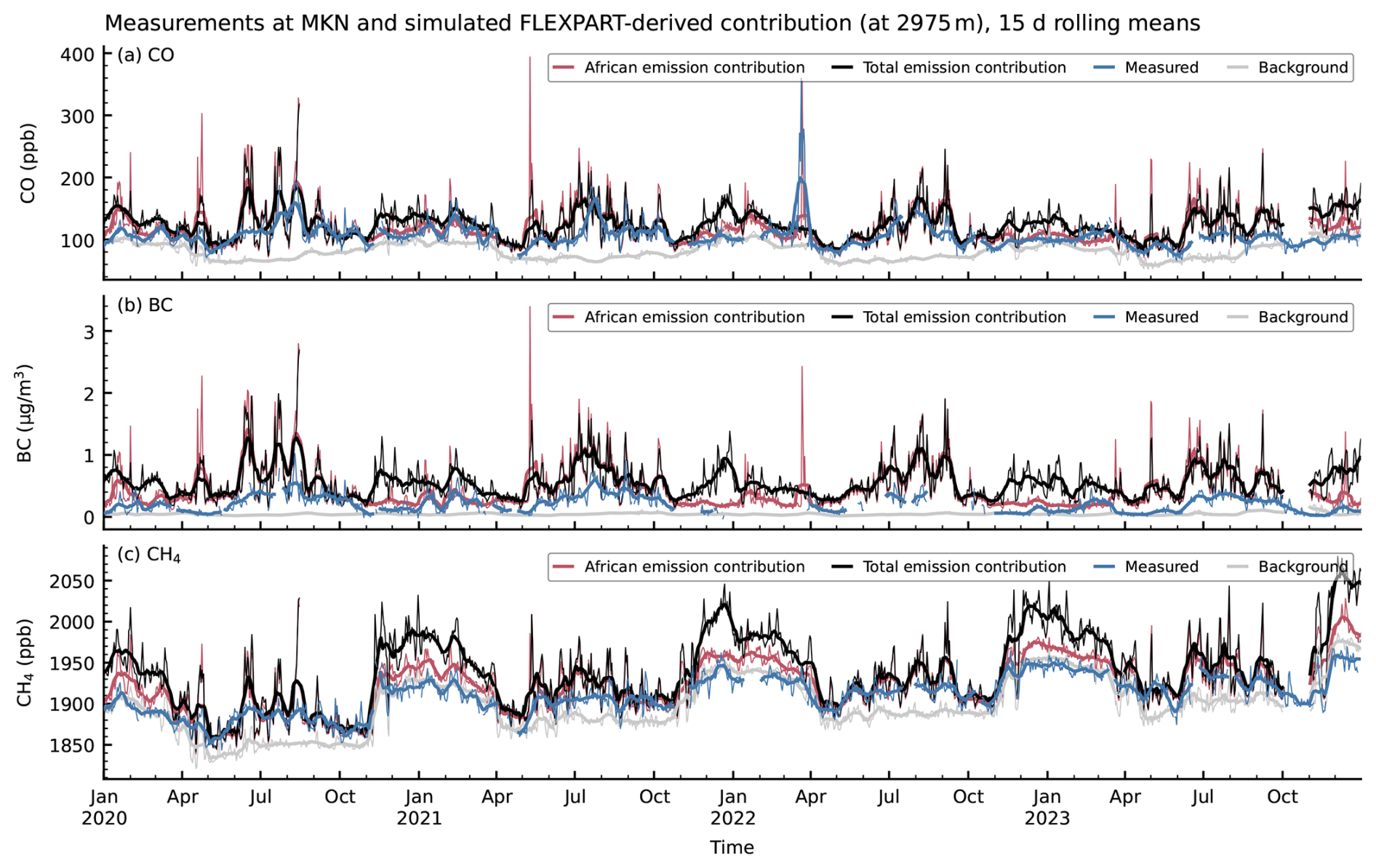
Figure 5 CO, BC and CH₄ measurements at Mt. Kenya and total simulated contributions accounting for fire, wetland, and anthropogenic emissions in the African domain (red) and the full domain (black). The background is derived from CAMS background data folded with FLEXPART footprints. Thin lines show daily averages, bold lines show data smoothed with a 15 d rolling mean.

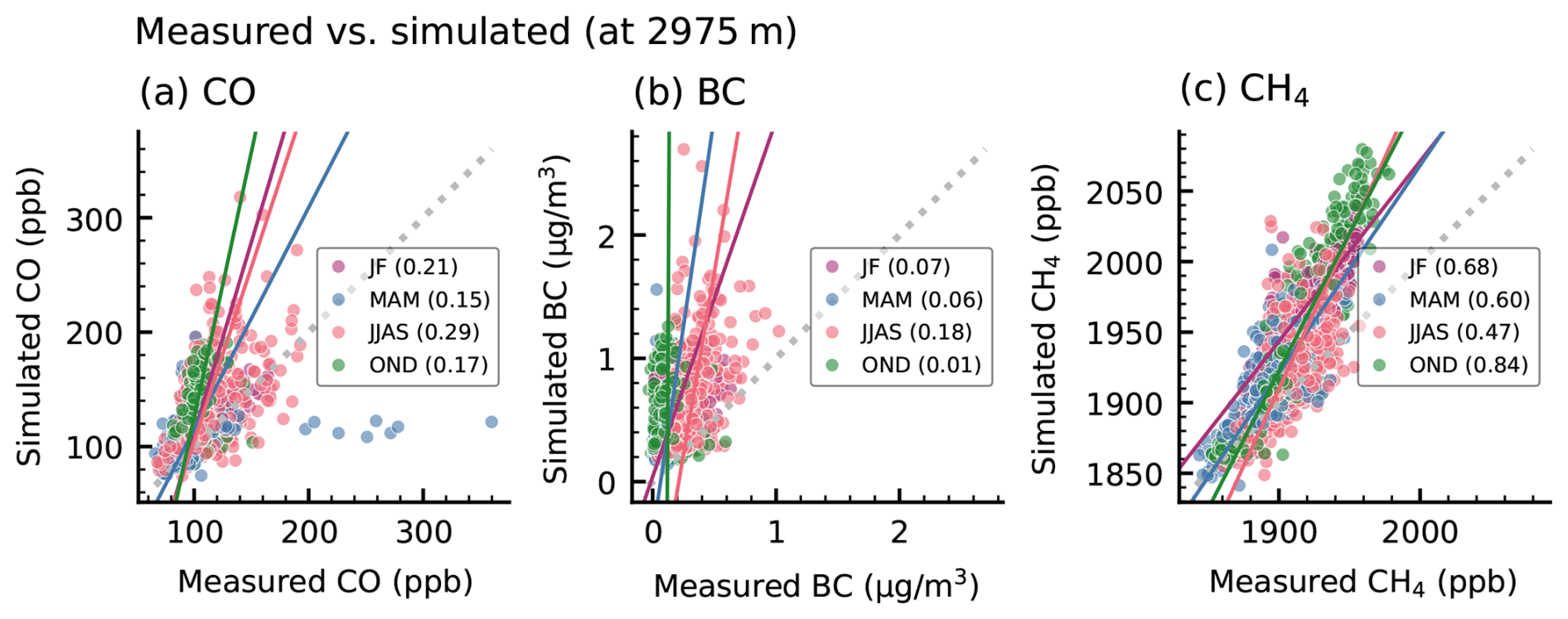
Figure 6 Scatter plots of measured (corresponding to the blue line in Fig. 5) versus simulated concentrations or amount fractions of the full domain (black line in Fig. 5) at MKN for CO, BC and CH₄ for all seasons. The grey dotted line shows the 1 : 1 fit, the thin coloured lines represent an orthogonal regression fit for each season. Values in the legend indicate the coefficients of determination R² for each season.

We observe good overall agreement between measured and simulated data for all three species, when transport and emissions are only accounted for the African domain (red line). However, when considering the full domain (black line), the simulated time series are mostly larger than observations. We saw that the largest contribution to this overestimation comes from anthropogenic EDGAR emissions, suggesting that the inventory overestimates emissions, not only in Africa but also from the larger domain. Figure 6 illustrates this overestimation of the simulated data, especially for CO and BC. Nevertheless, the correlation between observed and simulated BC and CO is weak in all months and the ODR model performs poorly for CO and BC, probably related to the large number of outliers (Fig. 6a, b). Furthermore, BC is treated in FLEXPART as an inert species neglecting scavenging, which likely explains why the model-observation agreement is worse for BC compared to CO, especially during the rainy seasons. Standard deviations of the measurements were considered for CO and CH₄ in the ODR fit, but were not available for BC, which might further explain the larger spread of the ODR fits for BC (Fig. 6b). Simulated CH₄ correlates better with the measurements (Fig. 6c) than CO and BC, but still slightly overestimates amount fractions in most months (Fig. 5c), for the full domain especially from December to March. This bias most likely results from overestimated emissions in the inventories or from an overestimated background. Indeed, the background (grey line in Fig. 5c) sometimes exceeds the measurements, indicating that simulated background values are too high.

As expected, we observe larger simulated contributions during the day (not shown), when the influence of PBL is largest, which is consistent with the results at Maïdo by Callewaert et al. (2022). However, comparing only day- or nighttime measurements with simulations hardly affects the overall correlation between modelled and simulated time series, suggesting that there is no major improvement when looking only at free-tropospheric or PBL contributions respectively.

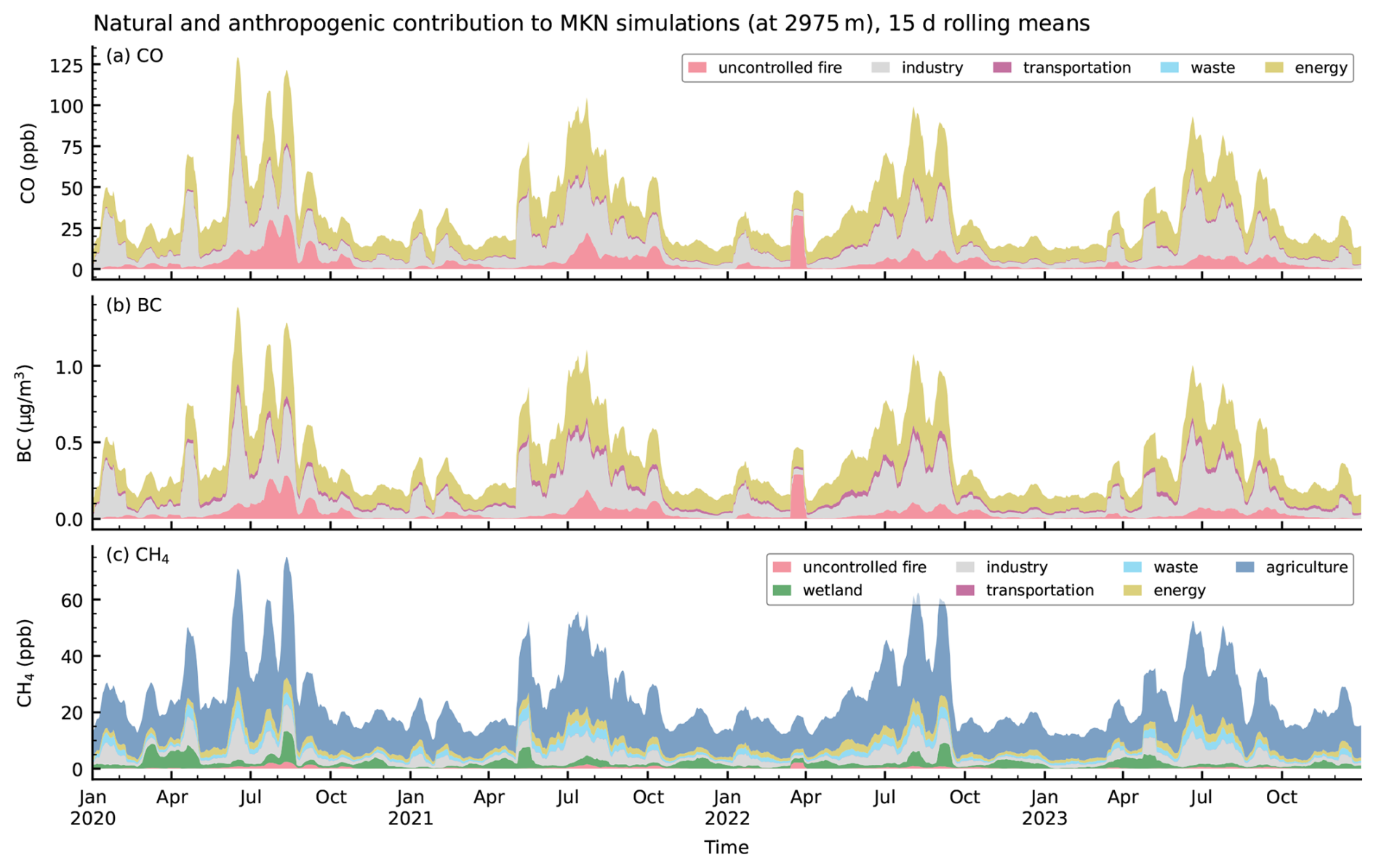
Figure 7 Simulated anthropogenic and natural emission contribution to MKN measurements above background and for various emission sectors, smoothed with a 15 d rolling mean.

The sectoral contributions from natural and anthropogenic emissions to the simulated time series are shown in Fig. 7, and their relative contributions for different seasons are shown in Fig. 8. Both figures concentrate on the African domain only, to investigate the effect of African emissions on MKN measurements. We observe that for CO and BC, the energy sector is the dominant contributor (around 46 %, see Fig. 8a, b), with contributions from the “energy for buildings”-group only. This represents solid fuel combustion for domestic and commercial energy production. The second largest contributing sector is industry (38 %), followed by uncontrolled fire (13 % for CO, 10 % for BC), with largest fire contributions around the dry season from June to October, and transportation. The fire sector here stands for uncontrolled burning detected by GFAS, in contrast to solid fuel burning for domestic energy production, which is part of the energy sector. As expected, CO and BC show very similar patterns, but the contribution from the transportation sector is slightly larger for BC (6 % for BC compared to 3 % for CO), due to larger shipping BC emissions.

As mentioned in Sect. 2.4.4, we use annual EDGAR inventories for anthropogenic emissions without seasonal variation. Our observed seasonal variability in anthropogenic emissions is thus only due to variations in atmospheric transport. For fire emissions, however, seasonal variations in atmospheric transport and emissions are considered.

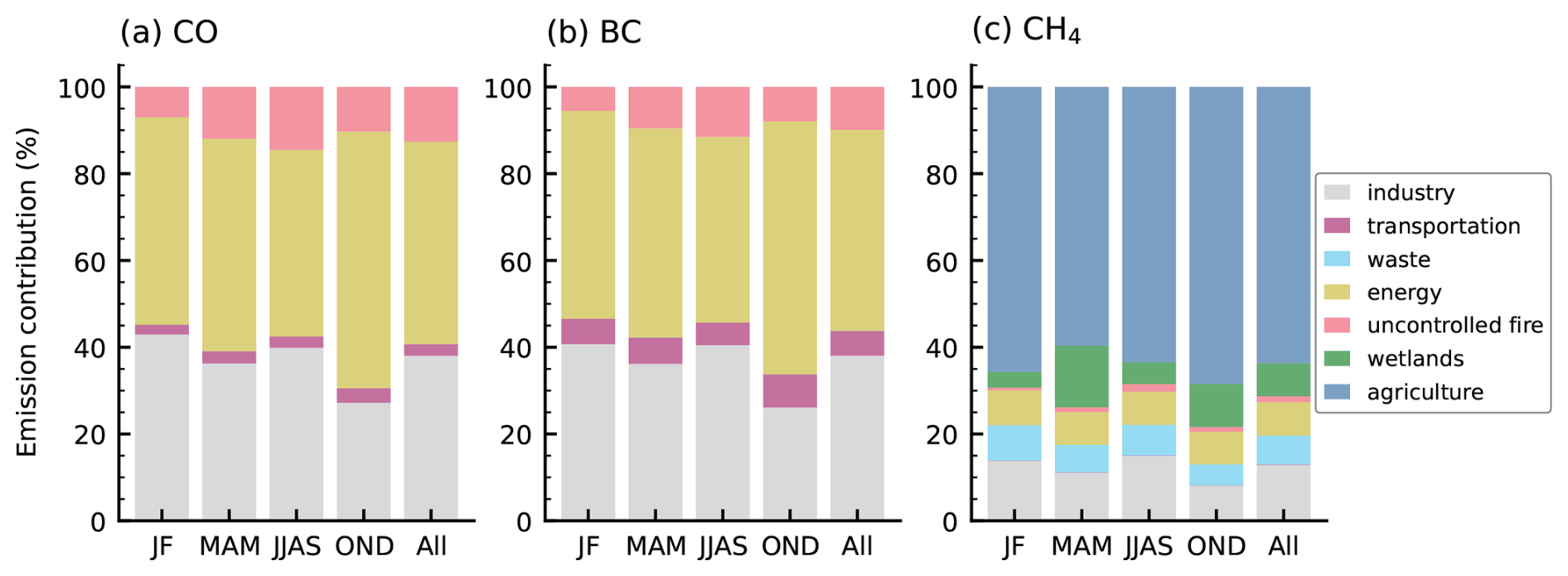
Figure 8 Relative sectorial contributions of simulated anthropogenic and natural emission to MKN measurements above background and for various emission sectors for different seasons and the whole time period (2020 to 2023).

For methane (Figs. 7c and 8c), the largest contribution comes from agriculture (64 %), which is mainly due to enteric fermentation, followed by industry (13 %), energy (due to fuel exploitation, 8 %), natural wetland emissions (8 %), waste (7 %), and uncontrolled fire (1 %). Wetland contributions, however, show a clear seasonal cycle, with contributions that exceed the ones from industry and energy during the wet seasons. In contrast to the anthropogenic emissions, the wetland seasonality is a combination of seasonal patterns in transport and emissions, because we use monthly resolved wetland inventory data.

Similar results for CH₄ were reported by Callewaert et al. (2022) at Réunion island, with dominating anthropogenic CH₄ contributions compared to wetland and fire. However, Dong et al. (2024) showed that emissions from one of the worldwide largest floodplain wetlands, the Sudd wetland in South Sudan, are highly underestimated, especially by the WetCHARTs product, due to the poor representation of wetland extent and dynamics. Even though the Sudd area is no major origin of air for MKN, their study indicates that wetland emissions may also be underestimated in our results.

In an ideal scenario, if the dispersion model and the inventories were perfect, the resulting simulated time series in Fig. 5 would perfectly match the measured concentrations at MKN. However, as discussed previously, inventories carry large uncertainties. Furthermore, like for any other dispersion model, tracer transport uncertainties in FLEXPART result from imperfect knowledge of the flow field (input fields) and approximations in the model formulation itself. Both uncertainties lead to differences between the observed and simulated time series.

Similar results have been reported by Callewaert et al. (2022), who modelled emission contributions to measured CO₂, CH₄ and CO at Réunion island. They found that EDGAR likely overestimates anthropogenic emissions.

Our overall agreement between measured and simulated time series suggests that the inventories for the African continent are broadly reliable in capturing underlying temporal patterns, which is an important insight for validation of regional emission inventories. However, in terms of absolute accuracy, the inventories are at the current state not good enough for accurate chemical modelling of the atmosphere (CO) or assessing the radiative forcing (BC). The underlying issues are well known, mainly related to the inaccurate and highly variable BC and CO emission factors for domestic energy production (cooking, lighting). More regional observations and a complete inversion analysis would be required to verify the quality of the inventories quantitatively. Due to the lack of continuous observations across the continent, this is not possible at the moment. Finally, it is important to note that the sectorial and seasonal variations are not representative for regional or African emissions, because they depend on the origin of air that is transported to MKN as considered by the FLEXPART dispersion model.

4 Conclusions

This study presents one of the most comprehensive multi-year datasets of in-situ trace gases and aerosol time series from equatorial Africa, measured at the high-altitude Global Atmosphere Watch (GAW) station Mt. Kenya (MKN). The results demonstrate the station's critical role in monitoring tropical atmospheric variability and trends, and for validating global models and emission inventories.

The trend analysis at Mount Kenya demonstrates that the detectability and interpretation of long-term changes strongly depend on the trace gas considered. For the well-mixed greenhouse gases CO₂ and CH₄, the MKN observations show clear and intensifying growth rates that are broadly consistent with global trends, confirming the suitability of this site for monitoring background concentrations in tropical Africa. In contrast, trends in the chemically reactive species O₃ and CO are weaker and more sensitive to period selection and regional processes. Ozone exhibits a modest long-term increase, but with evidence of a recent slowdown consistent with independent observations over East Africa, suggesting that regional photochemical production does not simply follow global free-tropospheric trends. CO trends are dominated by strong interannual variability related to biomass burning and climate modes such as ENSO, making robust long-term trend detection challenging despite the availability of continuous measurements. Together, these findings highlight that continuous observations at MKN provide unique constraints on tropical atmospheric variability and reveal important differences between greenhouse gases and shorter-lived species. They underscore both the value of sustained long-term measurements and the need for extended time series and additional stations across Africa to robustly separate long-term trends from climate-driven variability.

The observed seasonal cycles are strongly governed by the meridional migration of the Intertropical Convergence Zone (ITCZ), which modulates the origin of air masses and the associated trace gas and aerosol concentrations. Concentrations are generally lowest during the rainy seasons, when the ITCZ crosses the station in April/May and in November. CO, O₃ and BC peak during the southern biomass burning season from June to September, whereas CH₄ amount fractions show largest values in December/January, when northern continental air masses are dominant at MKN. Diurnal variability at the site is mainly driven by mountain dynamics, with upslope winds during the day transporting boundary layer air and downslope winds at night bringing free-tropospheric air to the station. This leads to distinct day–night differences in trace gas and aerosol particle concentrations, with nighttime measurements generally reflecting background conditions. The observed diurnal cycles are consistent across species, although CH₄ shows seasonally dependent patterns in the long dry season that require further investigation.

CAMS model data generally agree well with the measurements, but also reveal systematic underestimation of diurnal variability and seasonal dynamics, especially for ozone and black carbon during the rainy seasons. These discrepancies highlight the limitations of current model resolution and the importance of ground-based observations for improving atmospheric models.

The integration of FLEXPART dispersion modelling with bottom-up emission inventories allowed us to attribute observed variability to specific source sectors. CO amount fractions and BC concentrations are predominantly influenced by solid fuel burning emissions from the domestic energy and industrial sectors, and uncontrolled open biomass burning contributes to these species during the long dry season. Methane amount fractions beyond the hemispheric background are largely driven by agricultural emissions, with seasonal wetland contributions that are likely underestimated due to limitations in current wetland emission datasets. It is important to note that our results reflect the influence of air masses transported to the station and do not directly represent regional emissions. Systematic overestimation of the simulated concentrations highlight uncertainties and biases in both emission inventories and, to a lesser extent, transport modelling. Overall, our findings confirm the need for improved regional emission data and more comprehensive observational networks across Africa.

This study was conducted within the framework of the Horizon Europe KADI project, which aimed to strengthen Africa's climate knowledge base and support the development of a pan-African atmospheric observation system. It would not have been possible without prior persistent Kenyan and Swiss support of the station already 25 years ago, shortly after the official inauguration of the station. Sustained partnerships among national and international institutions, together with continuous capacity development and knowledge transfer, were key to successfully collecting the data and enabling the present analysis.

The long-term measurements at MKN provide critical insights into tropical atmospheric variability and demonstrate the value of sustained observations for model validation and emission inventory assessment. Furthermore, such long-term observations are indispensable to assess regional changes in greenhouse gas concentrations and to understand their variability in the context of a changing climate. In conclusion, the MKN station offers a unique and valuable perspective on tropical atmospheric variability, and its long-term measurements are essential for improving our understanding of regional variability and emissions, validating global models, and guiding future observational strategies.

Appendix A

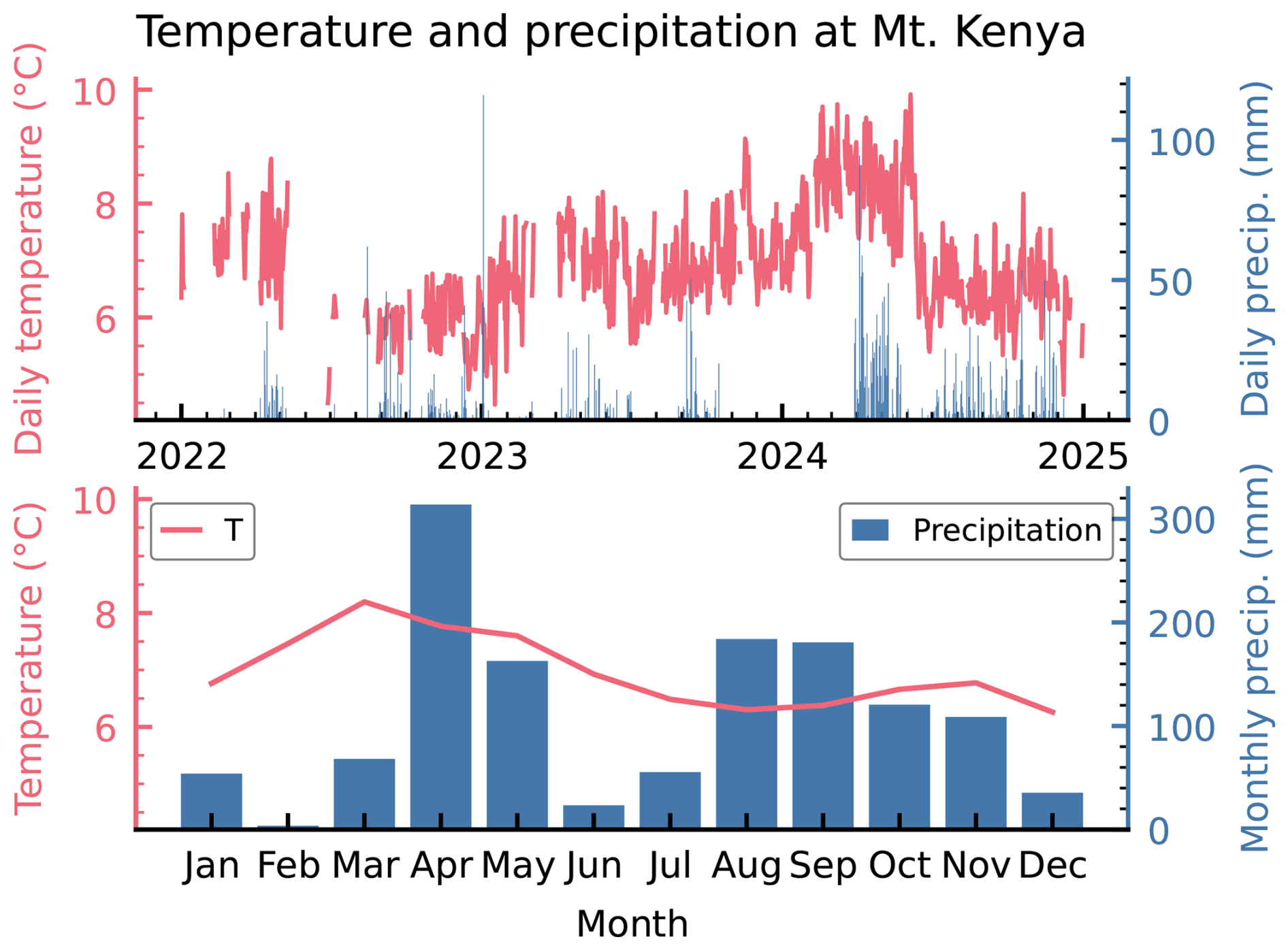
Figure A1 Measured temperature and precipitation data at the Mt. Kenya station for the period 2022 to 2024. The first panel shows daily temperature means and daily precipitation sums, for days with at least 18 hourly measurements available. The second panel shows monthly temperature means and monthly precipitation sums over the whole period.

Appendix B

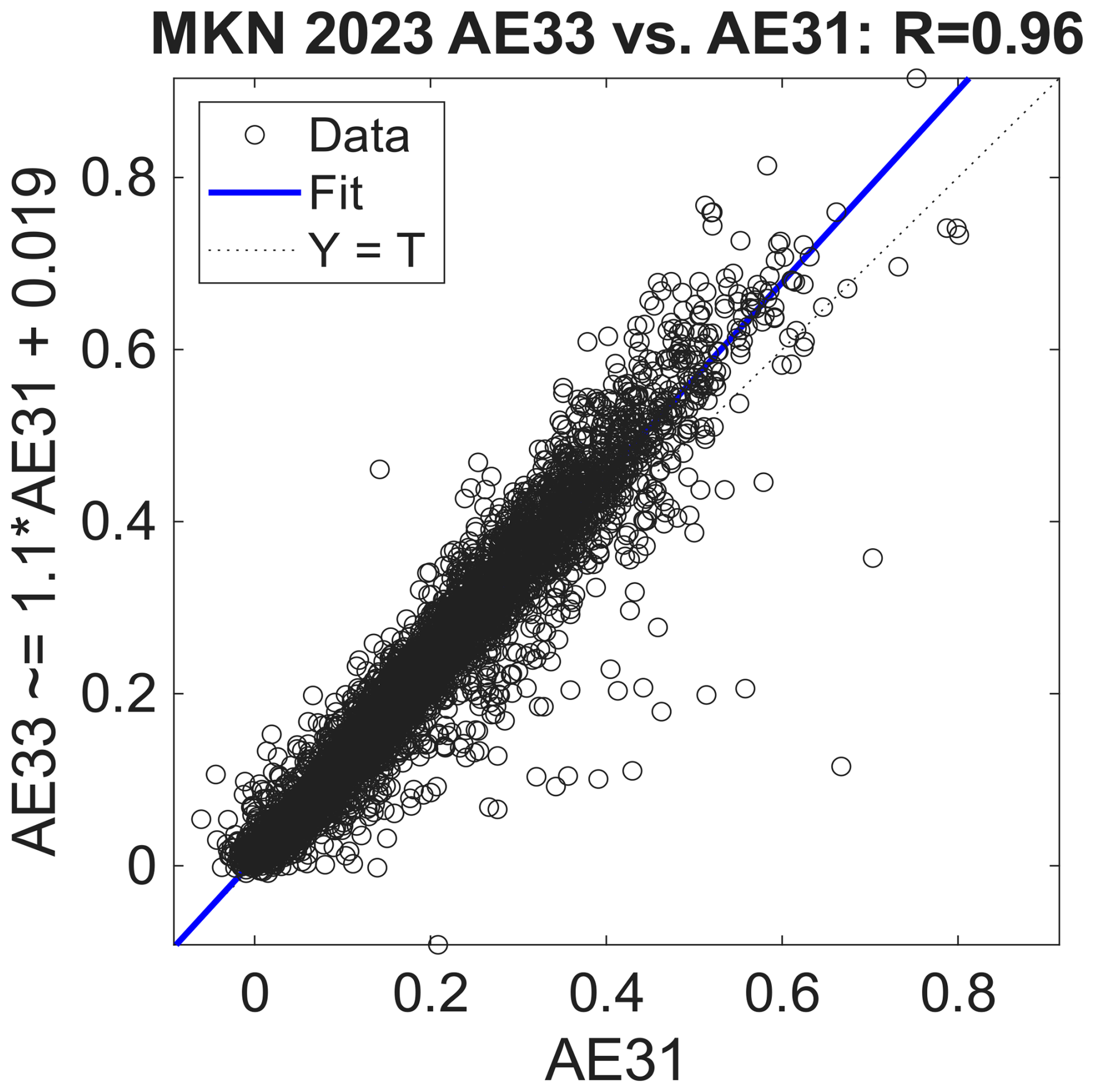
Figure B1 Comparison of equivalent black carbon (eBC) parallel measurements from two aethalometers (AE31 and AE33) in 2023 at MKN.

Appendix C

Table C1 Trends of CO₂ (in ppm yr⁻¹), CH₄ (in ppb yr⁻¹), O₃ (in ppb yr⁻¹) and CO (in ppb yr⁻¹) for different periods. Early and recent data for CO₂, CH₄ and CO are covering 2002 to 2011 and 2020 to 2024, respectively (see Fig. C1). For O₃, early and recent periods are 2002 to 2006 and 2015 to 2024. Trends ±2σ are calculated based on monthly aggregates.

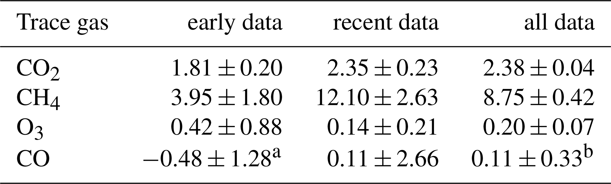
^a Derived from flask data (2004–2011). ^b Derived from flask data (2004–2011) plus continuous data (2020–2024).
The trend for all data (continuous (2002–2006), flasks (2008–2011), continuous (2020–2024)) is 0.63 ± 0.29 ppb yr⁻¹.

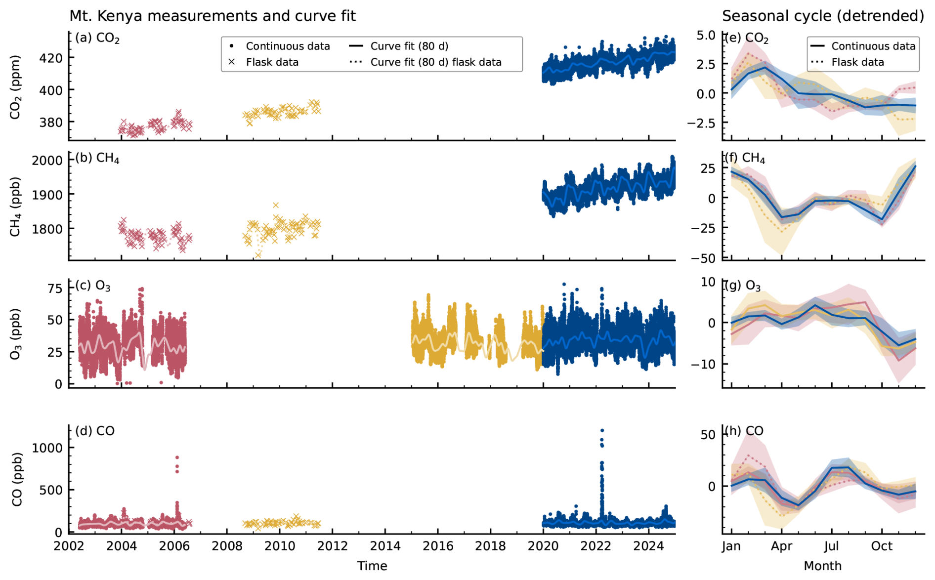
Figure C1 Long-term measurements including measurements prior to our analyses period. This includes early continuous O₃ and CO measurements, as well as NOAA flask measurements from 2003 to 2011. The data illustrate trends, challenges due to gaps, and good continuity since 2020. The seasonal cycles are shown for each of the 3 coloured time periods.