Processes driving the regional sensitivities of summertime PM_2.5 to temperature across the US: new insights from model simulations

The temperature sensitivity of fine particulate matter (PM_2.5) critically influences air quality and human health under a warming climate, yet models struggle to accurately reproduce observed sensitivities. This study improves the representation of PM_2.5-temperature relationships in the chemical transport model GEOS-Chem through targeted improvements and analyses of the underlying drivers based on simulations across the contiguous US (2000–2022). Our simulations reveal that chemical production processes, particularly isoprene secondary organic aerosol (SOA) and sulfate formation, determine the magnitude of PM_2.5 sensitivity in the eastern US. In the western US, primary emissions drive the increasing PM_2.5-temperature sensitivity. Transport processes contribute to interannual variability in PM_2.5 sensitivity across all regions. We quantified the contributions from individual temperature-sensitive processes for the first time. Sulfate concentration plays a pivotal role in modulating the sensitivity of isoprene SOA due to its direct influence on isoprene SOA formation. Furthermore, the increased SO₂ emissions on warm days dictates both the magnitude and variability of sulfate sensitivity in the eastern and central US. In the western US, however, sulfate sensitivity is primarily controlled by the temperature response of hydroxyl radicals (^•OH). These findings highlight the impact of anthropogenic emission reductions on declining PM_2.5–temperature sensitivity in the eastern US, improve our understanding of climate-driven air quality changes, and underscore the importance of accurately representing temperature-dependent processes in future air quality projections.

1 Introduction

Climate change represents one of the most crucial global challenges of the 21st century, adversely impacting human health through multiple pathways. These include exposure to extreme temperatures beyond habitual ranges, heightened food and water insecurity due to shifting average temperature and precipitation patterns, and the expanded transmission of infectious diseases in environments increasingly favorable to viruses (Romanello et al., 2021). Epidemiological studies reveal that a 1 °C rise in summer mean temperature correlates with an estimated 1 % and 2.5 % increase in mortality among older adults in the northeastern and southeastern US Medicare populations, respectively (Shi et al., 2015, 2016a). While numerous studies have explored the health impacts of climate change and the associated burden of rising temperatures (Achakulwisut et al., 2019; Costello et al., 2009; Ebi et al., 2021; Mora et al., 2017; Vicedo-Cabrera et al., 2021), one critical yet underexplored pathway is the health burden arising from climate-induced deterioration of ambient air quality.

Ambient air pollution, recognized as a leading environmental risk factor for global mortality, is suggested to play an increasingly important role in health outcomes under a warming climate (Murray et al., 2020). Among air pollutants, fine particulate matter (PM_2.5, particulate matter with an aerodynamic diameter less than 2.5 µm) is of particular concern due to its well-documented associations with increased all-cause mortality and elevated risks of cardiovascular, respiratory, and neurological diseases for both long-term and short-term exposure (Burnett et al., 2001; Cohen et al., 2017; Medina-Ramón et al., 2006; Shi et al., 2016b, 2020, 2023; Wang et al., 2017; Wei et al., 2019, 2020). PM_2.5 levels are controlled by primary and precursor emissions, photochemical reactions, transport, and deposition, and many of these factors are highly sensitive to temperature changes. Higher temperatures have often been associated with increased PM_2.5 pollution, a phenomenon termed the “climate penalty”, which reflects the potential deterioration of air quality due to warming in the absence of changes in anthropogenic activities (Bloomer et al., 2009; Duffy et al., 2019; Jacob and Winner, 2009; Schnell and Prather, 2017; Tai et al., 2010; Wu et al., 2008). This deterioration, in turn, adversely impacts human health and contributes to climate feedbacks via aerosol radiative effects. It is worth noting, however, that observational and modelling studies show that the sign and magnitude of this relationship vary substantially across regions, time periods, and PM_2.5 components, and are less consistent than those observed for tropospheric ozone.

PM_2.5 comprises several components, including sulfate, nitrate, ammonium, organic aerosols (OA), and elemental carbon (EC). The response of each component to temperature is governed by complex interactions of chemical and physical processes. Sulfate, for instance, forms through the gas-phase oxidation of sulfur dioxide (SO₂) and aqueous-phase oxidation of dissolved SO₂ in cloud droplets. Fossil fuel combustion remains the principal source of SO₂. Abel et al. (2017) found that the SO₂ emissions from power plants exhibited a 3.35 % ± 0.50 % increase per °C increase in summer months, attributed to heightened energy demand. While gas-phase oxidation of SO₂ accelerates at higher temperatures due to increased reaction rates, aqueous-phase oxidation exhibits competing effects: elevated temperatures enhance reaction rates but reduce dissolved gas concentrations due to equilibrium shifts, with cloud cover changes introducing further uncertainty (Xie et al., 2019). Nitrate is formed through the oxidation of nitrogen oxides (NO_x), and organic aerosols are generated both directly through combustion and indirectly via the atmospheric oxidation of non-methane volatile organic compounds (NMVOCs). Biogenic NMVOCs emissions are highly temperature sensitive (Guenther et al., 2012). Recent studies have suggested that emissions of anthropogenic NMVOCs can also increase with temperature (Pfannerstill et al., 2024; Qin et al., 2025; Wu et al., 2024). Both nitrate and organic aerosols are semi-volatile, with their partitioning between particle and gas phases strongly influenced by temperature. With warming and drought events intensifying wildfire activity, biomass burning emissions can be highly temperature sensitive, contributing to primary organic aerosol (POA) and EC. The formation of SOA is influenced by the presence of inorganic aerosols, such as sulfate and nitrate (Marais et al., 2016, 2017; Xu et al., 2015). The reactive uptake of semi-volatile or low-volatility organics into the aqueous phase introduces additional complexity to SOA temperature sensitivity. Xu et al. (2015) demonstrated that the isoprene-derived SOA and monoterpene SOA are directly modulated by the abundance of sulfate and NO_x, respectively. However, the extent to which anthropogenic pollutants impact the temperature sensitivity of biogenic SOA remains insufficiently explored. Beyond emissions and chemical production, temperature changes are associated with changes in meteorological factors such as ventilation (which is dependent on wind speed, mixing depth, convection, and frequency of frontal passages), precipitation, and atmospheric stagnation, all of which influence aerosol transport and removal rates, further modulating the PM_2.5 response to rising temperatures (Jacob and Winner, 2009).

Atmospheric aerosols play a critical role in modulating the Earth's energy balance by reducing the solar radiation that reaches the surface, thereby offsetting the greenhouse effect and slowing global warming. Understanding the interactions between climate and air pollution is crucial for predicting future climate scenarios and mitigating the adverse health impacts of climate change. Despite this importance, comprehensive studies on the temperature sensitivity of PM_2.5 remain limited, largely due to the complicated and diverse response of PM_2.5 components to temperature rises (Shen et al., 2017; Tai et al., 2010; Vannucci et al., 2024; Vannucci and Cohen, 2022; Westervelt et al., 2016). The relationship between elevated PM_2.5 levels and temperature is often quantified as the slope of the best-fit line between detrended PM_2.5 anomalies and temperature anomalies. Recent research has highlighted the decreasing temperature sensitivity of ammonium sulfate aerosols, accompanied by growing contributions from organic aerosols in recent years, driven by anthropogenic emission reductions (Hass-Mitchell et al., 2024; Nussbaumer and Cohen, 2021; Pfannerstill et al., 2024; Vannucci et al., 2024; Vannucci and Cohen, 2022). Our previous work, leveraging machine learning-derived high-resolution datasets combined with ground-based measurements, demonstrated widespread climate penalty effects across the contiguous United States (CONUS) (Yin et al., 2025). These effects show that the degradation of air quality due to rising temperatures has been partially mitigated by reductions in anthropogenic emissions, especially in the eastern US. However, while observations and machine learning provide insights into the overall temperature sensitivity of air pollution (e.g., ${\mathrm{dPM}}_{\mathrm{2.5}}/\mathrm{d}T$, $\mathrm{dsulfate}/\mathrm{d}T$, $\mathrm{dSOA}/\mathrm{d}T$), they cannot disentangle the contributions of individual processes. To address this, chemistry transport models (CTMs) can be helpful in decomposing total sensitivity into specific process contributions, such as precursor emissions ($\partial \left[\mathrm{sulfate}\right]/\partial \left[{\mathrm{SO}}_{\mathrm{2}}\right]\cdot \partial \left[{\mathrm{SO}}_{\mathrm{2}}\right]/\partial \left[T\right]$, $\partial \left[\mathrm{SOA}\right]/\partial \left[\mathrm{VOC}\right]\cdot \partial \left[\mathrm{VOC}\right]/\partial \left[T\right]$), chemical reaction rates ($\partial \left[\mathrm{sulfate}\right]/\partial \left[\mathrm{reaction}\mathrm{rate}\right]\cdot \partial \left[\mathrm{reaction}\mathrm{rate}\right]/\partial \left[T\right]$), transport and removal processes ($\partial \left[\mathrm{sulfate}\right]/\partial \left[\mathrm{transport}\right]\cdot \partial \left[\mathrm{transport}\right]/\partial \left[T\right]$), etc. By employing CTMs, these contributions may be dissected and quantified, potentially enabling a deeper understanding of the processes that govern temperature sensitivity and air quality.

Numerous studies have attempted to forecast air quality and the associated health risks under future climate conditions using global coupled climate-chemical models. However, these models often yield conflicting results, with disagreements even on the direction of future PM_2.5 changes (Jacob and Winner, 2009; Nolte et al., 2018; Vannucci et al., 2024). This variability underscores significant uncertainties in how climate change will affect air quality (West et al., 2023). The discrepancies among model results stem from challenges in projecting climate variables such as precipitation and cloud cover and capturing the temperature sensitivities of air pollution. For example, Shen et al. (2017) found that GEOS-Chem underestimated the temperature sensitivity of sulfate, potentially due to an overly sensitive response of cloud fractions to temperature in the meteorological fields. Given these limitations, it is essential to evaluate CTMs against observational data before relying on them for future projections. A model's ability to accurately resolve present-day relationships between climate variables and air quality serves as a robust criterion for identifying biases and building confidence in its application for forecasting future air quality responses to climate change (Fiore et al., 2012).

In this study, we evaluated the performance of the standard GEOS-Chem model in capturing the temperature sensitivity of PM_2.5 over CONUS. We implemented targeted model modifications to improve simulations and quantify the contributions of various temperature-sensitive processes. By identifying the primary drivers of PM_2.5 temperature sensitivity, this work advances our understanding of the complex interactions between climate, air quality, and health, thus providing greater confidence in projections of future air quality.

2 Methodology

2.1 Temperature Sensitivity Diagnosis

Following the methodology outlined by Fu et al. (2015), the sensitivity of air pollution to temperature was calculated as the slope of the linear regression line between detrended anomalies of air pollutant concentrations (e.g., ΔPM_2.5) and detrended temperature anomalies (ΔT). Interannual anomalies of pollutant concentration and temperature were derived by removing long-term means to eliminate apparent associations caused by overarching trends. For instance, a decreasing long-term trend in PM_2.5 coupled with an increasing temperature trend could create a misleading negative correlation, obscuring the true relationships between PM_2.5 and temperature driven by factors such as chemistry, emissions, and transport.

This study focused on the temperature sensitivity of ground-level PM_2.5 concentrations due to their direct implications for public health. Different regions in the CONUS were investigated separately to illustrate the spatial heterogeneity of pollutant-temperature relationships. The CONUS was divided into four regions (Fig. S1 in the Supplement): the Southeastern US, the Northeastern US, the Western US, and the Central US. The regional responses were obtained by regressing all detrended air pollution anomalies on temperature anomalies within each region. The study examined the temperature sensitivity of PM_2.5, as well as its five primary components, including sulfate, nitrate, ammonium, OA, and EC. The analysis utilized both ground-based observations from the Air Quality System (AQS) monitoring sites (for PM_2.5 and the five major components) and a high-resolution ground-level PM_2.5 concentration dataset generated through an ensemble machine-learning (ML) approach constrained by ground and satellite observations and by output from chemistry models (Di et al., 2019, 2021). Detailed descriptions of the AQS data, the ML dataset, the methodology for deriving temperature sensitivities, and the obtained results are provided in Yin et al. (2025). Overall, observational evidence reveals that a positive temperature sensitivity of summer PM_2.5 is pervasive across the continental US. While stringent emission control policies have markedly mitigated this sensitivity in the eastern US, an increasing temperature responsiveness of PM_2.5 has been observed in the western US. Temperature sensitivity values derived from observational and ML-modeled data were compared to those from GEOS-Chem simulations to evaluate model performance.

2.2 Evaluation of model performance with archived data

As a historical reference, we utilized archived outputs from an 18-year GEOS-Chem simulation (2000–2017) to evaluate the model performance in reproducing the temperature sensitivity of surface air pollution (Silvern et al., 2019a). The simulation was conducted using GEOS-Chem version 11-02c, driven by NASA MERRA-2 assimilated meteorological data. A nested simulation over North America was performed at a horizontal resolution of 0.5° × 0.625°, with dynamic boundary conditions obtained from a global simulation at a coarser resolution of 4° × 5°. Anthropogenic emissions for the US were based on the National Emission Inventory for 2011 (NEI 2011) and scaled to individual years using national annual scaling factors provided by the Environmental Protection Agency (EPA). Non-electricity generation NO_x emissions in NEI 2011 were reduced by 60 % for all years following Travis et al. (2016) to reduce model bias for NO_x, inorganic nitrate, and ozone simulations. Biomass burning emissions were derived from the daily Quick Fire Emissions Database (QFED) (Darmenov and da Silva, 2015). The simulation incorporated the complex SOA scheme, which accounts for the gas-phase oxidation of biogenic and anthropogenic volatile organic compounds (VOCs) and aqueous-phase oxidation of isoprene (Marais et al., 2016).

We focused on the model performance in simulating responses of summertime PM_2.5 to summer mean temperatures due to the strong positive correlation and their important implications for public health and climate projections (Yin et al., 2025). Figure 1 compares the temperature sensitivity derived from GEOS-Chem outputs (Fig. 1a2–a5) with diagnoses from ground-based observations and ML-modeled data for 2000–2016 (Fig. 1a1). To ensure comparability, all of these results were calculated based on 2000–2016 data, although more data are available for both observations and GEOS-Chem simulations. Maps showing only statistically significant results (p<0.05) are illustrated in Fig. S2. The results derived from the archived GC outputs are denoted as the “REF_2019” case. As shown in Fig. 1a2, the temperature sensitivities of PM_2.5 in the western and southeastern US derived from the REF_2019 case were significantly higher than results from observations and ML-modeled data. This overestimate was primarily driven by contributions from POA emitted by wildfires in the West and Central US and from SOA formed via aqueous-phase oxidation of isoprene in the Southeast and Northeast US (Fig. 1b1–b5). The similarly overestimated PM_2.5 and OA concentrations in the West and Southeast US (Figs. S3–S4) suggest that these discrepancies may stem from overestimated biomass burning emissions and uncertainties in the parameterization of isoprene SOA formation through aqueous-phase processes. Many studies have shown that QFED tends to overestimate fire emissions in the US, while the Global Fire Emissions Database (GFED) shows much better agreement with observed OA concentrations (Carter et al., 2020; Pan et al., 2020). Regarding the aqueous-phase oxidation of isoprene, Zheng et al. (2020) demonstrated that GEOS-Chem overestimates the dependence of acid-catalyzed reactive uptake of epoxy-diols (IEPOX) on inorganic aerosols, leading to an overestimated SOA concentration and exaggerated monthly variability. Additionally, the relatively low NH₃ emissions in August (compared to June and July) from NEI 2011 resulted in a highly acidic environment, which facilitates the aqueous SOA formation and contributes to the large simulated monthly variability (Fig. S5) (Zheng et al., 2020).

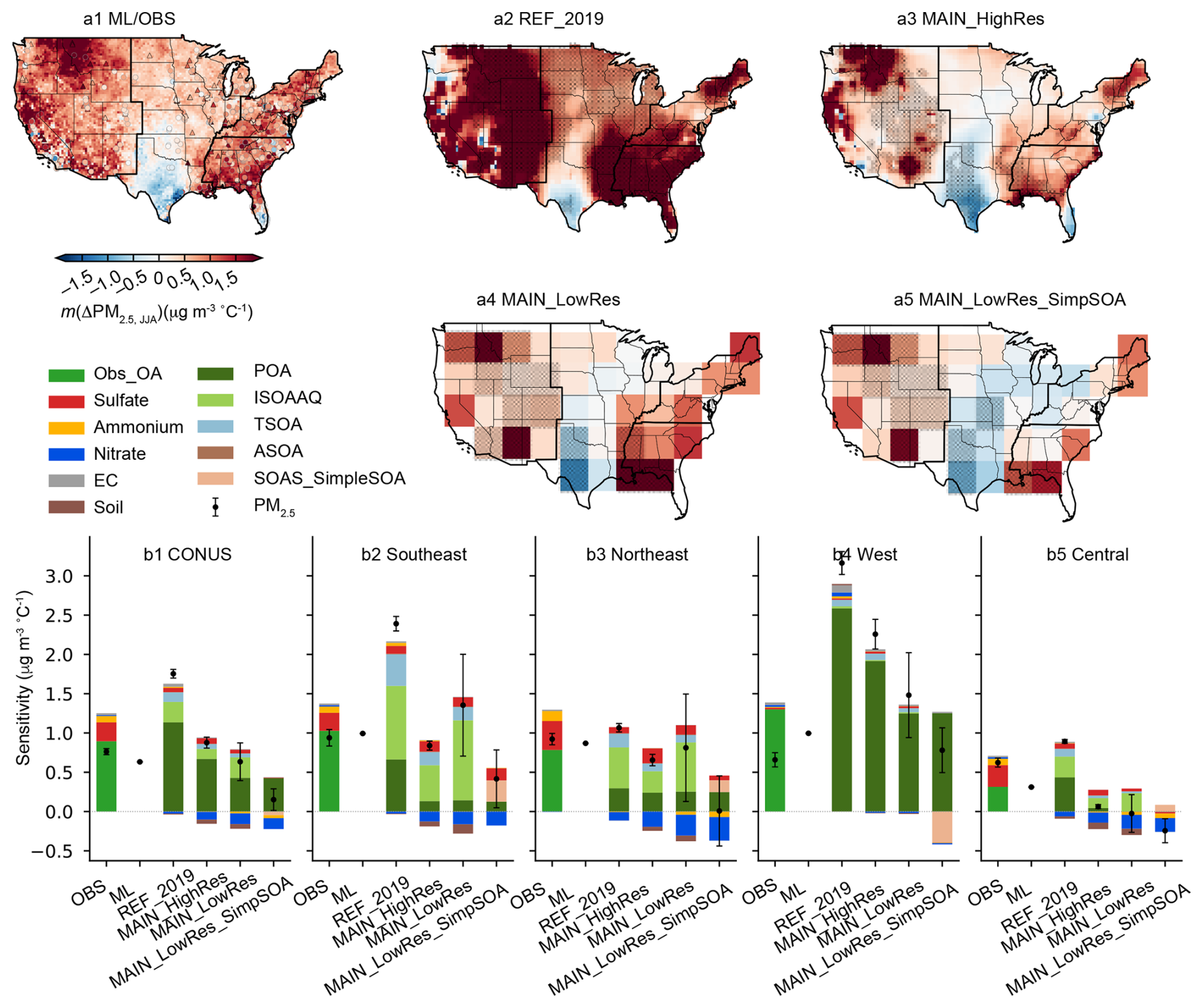
Figure 1 Spatial distribution and regionally aggregated temperature sensitivity of summertime PM_2.5 and its major components during 2000–2016, derived from ground-based observations, machine-learning (ML) modeled datasets, and GEOS-Chem simulations. Maps show the spatial distribution of PM_2.5 temperature sensitivity derived from ML-modeled data and observations (a1), GEOS-Chem REF_2019 case simulations (a2), MAIN_HighRes case simulations (a3), MAIN_LowRes case (a4), and MAIN_LowRes_SimpSOA case (a5). Triangle markers represent fitted sensitivities from observations with p-value < 0.05. Stippling represents fitted temperature sensitivities with p-value < 0.05 in GEOS-Chem. Bar charts show regionally aggregated temperature sensitivities for PM_2.5 and its major components across the contiguous United States (b1), the Southeastern US (b2), the Northeastern US (b3), the Western US (b4), and the Central US (b5).

In addition, in the REF_2019 case, the GEOS-Chem model underestimated the temperature sensitivity of sulfate in the US (Figs. 1b1–b5, S6–S7), despite reasonably reproducing sulfate concentrations (Figs. S3–S4). Shen et al. (2017) attributed this underestimation to the excessive sensitivity of cloud fraction in GEOS-5 assimilated meteorological data (used in older versions of GEOS-Chem) to temperature. This exaggerated response leads to a rapid decrease in cloud fraction with rising temperatures, reducing aqueous-phase sulfate production and resulting in a negative correlation between sulfate concentrations and temperature in GEOS-Chem simulations. However, the MERRA-2 meteorological data used in this study show a weak cloud cover response to temperature rise (∼ 0.01 K⁻¹, Fig. S8), more consistent with the satellite-derived results than GEOS-5 (Shen et al., 2017). For SO₂ emissions from electricity generation, the GEOS-Chem model relies on the NEI, which adopts data from the Power Sector Emissions Data collected by the EPA's Clean Air Markets Division (CAMD, https://campd.epa.gov, last access: 20 April 2026). However, the NEI scaling factors for individual years do not fully capture interannual variations in SO₂ emissions from power plants, which are often temperature dependent. Figure S9 shows that the national variations used to scale NEI 2011 SO₂ emissions fail to align with the raw CAMD data, potentially limiting the model's ability to reproduce the observed temperature sensitivity of sulfate. To address this, we replaced the default GEOS-Chem scaling method for NEI, which applies uniform annual scaling factors across all months and regions, with a more detailed approach. In brief, year-to-year variations in monthly SO₂ emissions for each subregion were derived from CAMD data and incorporated into the simulations. Figure S10 illustrates the time series of SO₂ and NO_x emissions during June, July, and August for four subregions in the CONUS. The northeastern US exhibited the highest emissions, followed by the Central US, Southeast, and West. These region-specific monthly variations are expected to enhance the model's capability to capture the temperature sensitivity of sulfate more accurately.

2.3 Model setup

To address the potential sources of discrepancies mentioned above and improve the performance of GEOS-Chem in estimating temperature sensitivity, we conducted a new simulation covering 2000–2022 with GEOS-Chem version 12.9.3 (https://doi.org/10.5281/zenodo.3974569, International GEOS-Chem User Community, 2020). The nested simulation at 0.5° × 0.625° horizontal resolution over the US was conducted with dynamic boundary conditions from a global simulation with 4° × 5° horizontal resolution. The model is driven by offline meteorology from NASA MERRA-2. Global anthropogenic emissions are derived from the Community Emissions Data System (CEDS) inventory (https://doi.org/10.5281/zenodo.4741285, O'Rourke et al., 2021), with the US region replaced by NEI 2016 to address the large discrepancies in NH₃ emissions between August and June–July (Fig. S5). Monthly mean anthropogenic emissions were scaled from 2016 to the simulated year using the EPA's national annual scaling factors, except for SO₂ and NO_x emissions from the power sector, which were scaled based on the CAMD annual trends, as described earlier (Fig. S10). Biomass burning emissions were obtained from GFED version 4 (Randerson et al., 2017). Biogenic emissions of isoprene and terpenes were calculated using the Model of Emissions of Gases and Aerosols from Nature (MEGAN2.1) (Guenther et al., 2012). The ISORROPIA II thermodynamic model is employed to estimate aerosol water content and aerosol acidity (Fountoukis and Nenes, 2007).

We employed the complex SOA scheme in GEOS-Chem with specific modifications to improve SOA modeling. The complex scheme utilizes a more advanced volatility basis set approach for non-isoprene SOA, incorporating an explicit aqueous uptake mechanism for isoprene SOA (Marais et al., 2016). The semi-volatile POA was disabled by default in the model configuration. A study assessing model performance across different OA schemes found that the non-volatile POA treatment more accurately reproduces the low-tropospheric POA profile compared to the semi-volatile approach (Pai et al., 2020a). Additionally, since oxidized POA is not included in the SOA mass, disabling the semi-volatile POA scheme does not impact SOA simulation results and helps reduce computational costs. The default aqueous-phase isoprene SOA formation scheme in GEOS-Chem did not account for the mixing of inorganic aerosols with organics, which is common in the real atmosphere (Li et al., 2021; Riva et al., 2016). This omission can lead to overestimations, as organic coatings on aerosols may suppress the uptake of IEPOX onto acidified sulfate aerosols (Riva et al., 2016; Schmedding et al., 2019; Zhang et al., 2018). To address this, we implemented the linear coating effect following the method described by Zheng et al. (2020) for IEPOX-SOA formation. This modification aims to reduce the overestimated SOA concentration and its sensitivity to inorganic aerosols present in the default GEOS-Chem setup. Additionally, we fixed the aerosol acidity $a_{{\mathrm{H}}^{+}}$ level at 0.1 mol L⁻¹ for the IEPOX uptake rate calculation, based on findings from Zheng et al., (2020), which demonstrated the best agreement with observed SOA levels in the southeastern US. Importantly, the aerosol acidity level was fixed only for the IEPOX uptake process and did not affect other chemical processes in the model.

GEOS-Chem also includes a simple SOA scheme, which treats POA as non-volatile and employs a fixed-yield approach for SOA formation. Despite their differing levels of complexity, the simple and complex schemes have demonstrated comparable performance in capturing overall OA magnitudes (Pai et al., 2020b). To assess the ability of these two schemes to reproduce the temperature sensitivity of PM_2.5, we conducted simulations using the simple SOA scheme. This simulation was performed at a coarser horizontal resolution of 4° × 5° for the period 2000–2017, matching the resolution of the boundary condition (BC) simulations used in nested simulations for other cases. Table 1 provides a summary of all simulation cases conducted in this study. Although total simulation durations vary across cases, all comparisons with ML-based results and observations are restricted to their overlapping periods to ensure temporal consistency.

Table 1 Case configurations used in this study.

3 Results

3.1 Model evaluation

The observed and simulated spatial distribution and regional mean of summertime PM_2.5 and its species concentrations during 2000–2022 are shown in Figs. S3–S4. The simulated regional means were calculated based on grid points co-located with observation sites. Two primary metrics were used in this study to evaluate model performance against ambient observations: the coefficient of determination (r²) and the root-mean-square error (RMSE). The r² metric represents the proportion of variance in observational data that is accurately captured by the model, while RMSE quantifies the average magnitude of differences between simulations and observed data. A comparison of these metrics across four cases is shown in Fig. S11. The main GEOS-Chem (MAIN_HighRes) case outperformed the REF_2019 case for most PM_2.5 species, demonstrating higher r² values and lower RMSE. For nitrate, however, the RMSE of MAIN_HighRes is 30 % higher than that of the REF_2019 case in the CONUS, likely due to improved NO_x emissions used in REF_2019 simulations (Silvern et al., 2019a). However, accurate measurements of nitrate are challenging due to its temperature-sensitive thermodynamic equilibrium. The EPA's Federal Reference Method (FRM) standard for sampling PM has been shown to underestimate PM_2.5 concentrations, primarily due to the volatilization of aerosol nitrate from filters (Hering and and Cass, 1999; Ward et al., 2025). OA metrics are significantly improved in the Southeast, West, and Central US, with r² ranging from 0.63 to 0.80. Across the CONUS, the r² of OA improved markedly from 0.30 in the REF_2019 case to 0.68 in the MAIN_HighRes case. The higher RMSE for OA simulations in certain regions can be attributed to overestimated concentrations in 2021. This discrepancy is likely driven by exceptionally high wildfire emissions within the GFED4 inventory for certain years, such as 2021 (Fig. S4). Because wildfire-driven OA is strongly temperature dependent and spatially heterogeneous, these overestimations can disproportionately affect regression-based temperature sensitivity diagnostics. Additionally, potential under-sampling by ground-based monitors near fire zones may lead to an underestimation of regional mean concentrations in observational datasets. Furthermore, current CTMs face inherent challenges in capturing the non-linear chemistry and rapid transport associated with extreme fire events (Qiu et al., 2024). Despite these uncertainties, data from high-fire years were retained in the full record, as they represent the growing influence of extreme wildfire events on air quality in a warming climate and reflect an important stress test for current modelling frameworks. In general, the modified GEOS-Chem model demonstrates reasonable accuracy in simulating concentrations of PM_2.5 and its components, supporting its suitability for diagnosing temperature sensitivity.

3.2 Model performance in temperature sensitivity simulation

As shown in Fig. 1a3, the magnitudes of the simulated sensitivity of summertime (JJA) PM_2.5 to summertime temperature in 2000–2016 by the modified GEOS-Chem were significantly reduced, bringing them closer to the machine-learning and observation-derived results. For the CONUS, the PM_2.5 sensitivities across the four cases REF_2019, MAIN_HighRes, MAIN_LowRes, and MAIN_LowRes_SimpSOA are 1.75, 0.88, 0.63, and 0.15 µg m⁻³ °C⁻¹, respectively. In comparison, ML-derived and observation-derived PM_2.5 sensitivities are 0.63 and 0.76 µg m⁻³ °C⁻¹, respectively.

The PM_2.5 sensitivity is significantly reduced in the MAIN_HighRes case in all subregions. Specifically, in the Southeast US, the PM_2.5 sensitivity was reduced from 2.39 µg m⁻³ °C⁻¹ in REF_2019 to 0.75 µg m⁻³ °C⁻¹ in MAIN_HighRes, better aligning with the ML-derived and observation-derived values of 0.99 and 0.94 µg m⁻³ °C⁻¹, respectively. The temperature sensitivity of POA and aqueous-phase formed isoprene SOA (ISOAAQ), two key drivers of OA sensitivity and overall PM_2.5 sensitivity, decreased by approximately 80 % and 50 %, respectively, in the MAIN_HighRes case compared to the REF_2019 case. In the Northeast, the POA sensitivities remained consistent across cases, but the ISOAAQ sensitivity decreased from 0.52 in the REF_2019 case to 0.27 µg m⁻³ °C⁻¹ in the MAIN_HighRes case. In the West, the temperature sensitivity of POA dominates PM_2.5 sensitivity. The MAIN_HighRes case estimated a POA sensitivity of 1.92 µg m⁻³ °C⁻¹, substantially reducing the overestimation observed in the REF_2019 case. In the Central US, the POA and ISOAAQ sensitivities decreased from 0.44 and 0.26 µg m⁻³ °C⁻¹ in the REF_2019 case to 0.04 and 0.13 µg m⁻³ °C⁻¹ in the MAIN_HighRes case, respectively. These reductions in POA and ISOAAQ sensitivities contribute to narrowing the discrepancy between observed/ML-derived PM_2.5 sensitivities and standard GEOS-Chem simulations. This highlights the effectiveness of incorporating GFED4s for wildfire emissions and accounting for coating effects in aqueous SOA formation from IEPOX uptake in improving temperature sensitivity simulations.

In the MAIN_HighRes case, we incorporated the annual variation in SO₂ emissions from electricity generation units to enhance the simulation of sulfate temperature sensitivity. As shown in Fig. 1b1, the temperature sensitivity of sulfate in the CONUS increased by 40 % in the MAIN_HighRes case (0.07 µg m⁻³ °C⁻¹) compared to the REF_2019 case (0.05 µg m⁻³ °C⁻¹), with the most notable improvement observed in the Northeast, where the sensitivity was twice as high in the MAIN_HighRes case. In the Southeast, the sulfate sensitivity increased from 0.10 to 0.13 µg m⁻³ °C⁻¹. Despite these improvements, the MAIN_HighRes case still underestimated sulfate sensitivity by 42 %, 49 %, and 74 % in the Southeast, Northeast, and Central US, respectively. In the Western US, sulfate sensitivity remained negligible (0.02 µg m⁻³ °C⁻¹) across both simulations and observations. While using CAMD-derived scaling factors improved sulfate sensitivity simulations to some extent, a more accurate representation of the temperature dependence of SO₂ emissions and sulfate formation is needed for further refinement. Additionally, the parameterization of temperature-sensitive processes related to sulfate concentrations should be improved to better capture the observed high sensitivities. The low regional sulfate sensitivity may also result from subregional aggregation, which includes both urban and rural areas. Most ground-based stations are located in urban areas, where sulfate is more temperature-dependent due to higher energy consumption. However, as shown in the spatial distributions of species' temperature sensitivity (Figs. S6–S7), GEOS-Chem systematically underestimated sulfate sensitivity at most sites in the eastern US, particularly in the Northeast and Appalachian regions.

Nitrate concentrations are observed to exhibit minimal sensitivity to temperature changes, whereas the model estimates a strong negative correlation between nitrate and temperature (Fig. 1b1–b5). Using satellite-derived NO_x emissions in the REF_2019 case partially mitigated this issue, but strong negative correlations persist across much of the central and eastern US (Figs. S6–S7). One plausible explanation is that the temperature dependence of NO_x emissions is not adequately represented in the emission inventories and scaling factors, making it challenging for the model to reproduce the observed positive correlation. Additionally, the gas-particle phase partitioning of nitrate in GEOS-Chem appears overly sensitive to temperature, reinforcing the strong negative relationship, which competes with the positive correlation expected from emissions (Shen et al., 2017). Evaporation artifacts in nitrate measurements, which affect absolute concentrations, may also introduce bias in the calculation of temperature sensitivity. As the ammonium concentration tracks sulfate and nitrate, the model also simulated negative correlations between ammonium and temperature in the eastern US, driven by the strong negative response of nitrate to temperature. In contrast, observations indicate positive correlations for ammonium. The temperature sensitivity of EC and dust is negligible in both observations and simulations, consistent across the analyzed regions.

The role of complex SOA formation schemes in temperature sensitivity simulations can be investigated by comparing the MAIN_LowRes case and MAIN_LowRes_SimpSOA case. In the MAIN_LowRes case, which employed the complex SOA scheme, the temperature sensitivity of SOA is primarily driven by ISOAAQ, with a smaller contribution from monoterpene SOA (TSOA). By contrast, the simple SOA scheme in the MAIN_LowRes_SimpSOA case represents total SOA concentrations as a single variable (SOAS). The overall SOA sensitivity in the MAIN_LowRes case is 0.31, 1.19, 0.71, 0.07, and 0.26 µg m⁻³ °C⁻¹ in the CONUS, Southeast, Northeast, West, and Central US, respectively. These values compare to sensitivities of −0.05, 0.27, 0.15, −0.39, and 0.09 µg m⁻³ °C⁻¹ in the MAIN_LowRes_SimpSOA case. Our findings indicate that, while the simple SOA scheme performs reasonably well in reproducing observed PM_2.5 and OA concentrations (Figs. S4 and S11), it fails to capture the temperature dependence of SOA formation. This limitation suggests that using the simple scheme for predicting air pollution levels under future climate scenarios could result in significant discrepancies, particularly in regions where temperature-driven processes strongly influence SOA production.

3.3 Long-term variabilities of PM_2.5 temperature sensitivity

We further investigated the model performance in reproducing the variability of temperature sensitivity of PM_2.5 and its species. Figure 2 shows the 5-year rolling windows of temperature sensitivity for summertime PM_2.5 derived from observations, ML-modeled data, and four GEOS-Chem cases. The sensitivities of two key species, sulfate and OA, are also included in Fig. 2. Figure S12 shows the variability for summertime ammonium, nitrate, and BC sensitivity. The results reveal that the REF_2019 case consistently overestimated PM_2.5 sensitivity in the Southeast and the West across all 5-year windows from 2000 to 2017. By contrast, the MAIN_HighRes case significantly reduced this overestimation, accurately capturing both the magnitude and variability of PM_2.5 sensitivity in each subregion.

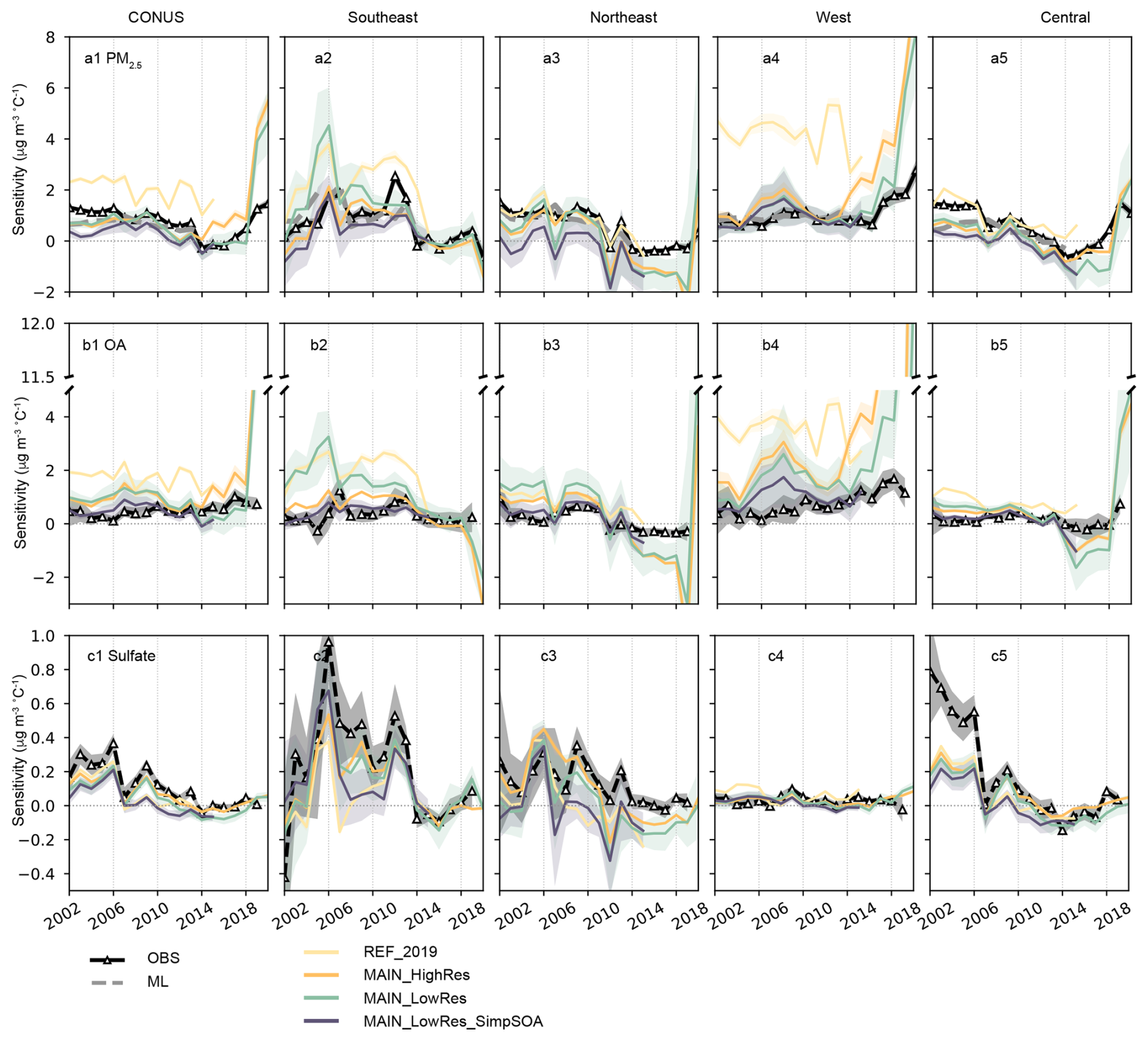
Figure 2 Regional-aggregated temperature sensitivity of PM_2.5, organic aerosols (OA), and sulfate for 5-year running time windows, derived from ground-based observations, machine-learning-modeled data (2000–2016), and four GEOS-Chem simulation cases. The shaded areas represent the 95 % confidence interval across each region. Panels (a1)–(a5) show the PM_2.5 sensitivity for the contiguous US (a1), the Southeast US (a2), the Northeast US (a3), the West US (a4), and the Central US (a5); (b1)–(b5) show the OA sensitivity for each region; (c1)–(c5) show the sulfate sensitivity for each region.

In the Southeast, observed PM_2.5 sensitivities to temperature in 2000–2013 were relatively high, ranging from 0.15 to 2.54 µg m⁻³ °C⁻¹ with substantial interannual variations. After 2014, the PM_2.5 sensitivity stabilized at lower levels, ranging from −0.63 to 0.39 µg m⁻³ °C⁻¹. Two notable peaks were observed during 2004–2008 and 2008–2012, which coincided with peaks in OA and sulfate sensitivities. Since the primary source of OA sensitivity in the Southeast is ISOAAQ, the formation of which is sensitive to the sulfate concentrations, the OA sensitivity could also be affected by the sulfate sensitivity. Both the REF_2019 and MAIN_HighRes cases captured sulfate sensitivity peaks in 2006 and 2012 (Fig. 2b2, c2). However, the REF_2019 case exhibited exaggerated OA sensitivity with two pronounced peaks during this period, resulting in substantial overestimation of both OA and PM_2.5 sensitivities. This result aligns with findings by Zheng et al. (2020), which highlighted that the ISOAAQ formation in GEOS-Chem is overly sensitive to sulfate concentrations. Incorporating the coating effects in the MAIN_HighRes case effectively reduced these discrepancies, yielding more accurate simulations of OA and PM_2.5 sensitivities.

In the Northeast, observed PM_2.5 sensitivity to temperature decreased from 1.53 µg m⁻³ °C⁻¹ during 2000–2004 to −0.32 µg m⁻³ °C⁻¹ during 2012–2016 and has remained at low levels since then. The MAIN_HighRes case successfully reproduced the overall decreasing tendency, except for a significant overestimation during 2017–2022, primarily driven by overestimated OA sensitivity in this region (Fig. 2b3). This discrepancy may be attributed to high POA emissions in the GFED4 inventory for 2021 (Fig. S4). Observed OA concentrations in the Northeast exhibit minimal temperature sensitivity from 2000 to 2011, ranging from 0.06 to 0.96 µg m⁻³ °C⁻¹. After 2011, observations show a negative relationship between OA and temperature, with sensitivities ranging from −0.03 to −0.34 µg m⁻³ °C⁻¹. The GEOS-Chem cases reasonably captured this transition, with an average OA sensitivity of 0.75 µg m⁻³ °C⁻¹ before 2011 and −0.53 µg m⁻³ °C⁻¹ afterward. Observed sulfate sensitivity in the Northeast shows a decreasing tendency from 2000 to 2013, stabilizing at approximately 0.01 µg m⁻³ °C⁻¹ in recent years. This decrease is primarily driven by efficient emission controls implemented in the eastern US during the study period (Yin et al., 2025).

In the western US, observed PM_2.5 sensitivity shows a substantial increase after 2014. The MAIN_HighRes case shows good consistency with observed data from 2000–2016, while overestimating PM_2.5 sensitivity in the western US from 2016–2022 (Fig. 2a4, b4), which could also be attributed to the high OA concentrations during this period (Fig. S4). These results highlight that short-term temperature sensitivity diagnoses are inherently susceptible to single-year emission or concentration anomalies, as shortening the analysis window increases the leverage of such outliers. This underscores the critical need for accurate representation of temperature-dependent processes in emission inventories – particularly for primary pollutants – within sensitivity simulations. For OA, this specifically requires a robust representation of temperature-sensitive burned area during emission estimation. Furthermore, we conducted a 10-year rolling window analysis (Fig. S13) to assess long-term stability. As expected, the longer time window smooths the interannual variability, demonstrating that the underlying signals of anthropogenic mitigation (in the East) and climate penalty intensification (in the West) are robust and persist despite the noise introduced by the 2021 fire anomaly. Consequently, the substantial fluctuations observed in the 5-year analysis reflect the high leverage that extreme events exert on short-term regressions rather than a lack of robustness in the underlying model framework. As this study aims to move beyond the long-term patterns to focus on interannual variability and its specific drivers, retaining the 2021 data can also help identify and quantify the role of wildfire emissions in temperature sensitivity simulations.

In the Central US, observed PM_2.5 sensitivity decreased from 1.46 µg m⁻³ °C⁻¹ during 2000–2004 to −0.63 µg m⁻³ °C⁻¹ during 2012–2016 and then increased to 1.09 µg m⁻³ °C⁻¹ during 2018–2022 (Fig. 2a5). As shown in Fig. 2c5, the decrease before 2016 was mainly driven by declines in sulfate sensitivity, whereas the OA sensitivity remained stable during this period. After 2016, sulfate sensitivity increased slightly by ∼ 0.17 µg m⁻³ °C⁻¹, and OA increased by ∼ 0.73 µg m⁻³ °C⁻¹, dominating the increases of PM_2.5 sensitivity from 2016 to 2022 (Fig. 2b5). Similar to the OA sensitivity observed in the western US, the increased OA sensitivity in the Central US may also be associated with wildfire emissions, reflecting the growing influence of wildfires on both regional and national air quality (Burke et al., 2023). The MAIN_HighRes case reproduced variabilities for both PM_2.5 and its species, although it underestimated sulfate sensitivity during 2000–2006. Notably, PM_2.5 sensitivity derived from ML-modeled datasets is lower than that from ground-based observations and more closely matches the GEOS-Chem simulations. The low spatial coverage of ground monitoring sites in the Central US makes observed PM_2.5 sensitivity less representative of the broader regional response; it also means that the ML-modeled dataset is likely more influenced in this region by the chemistry models used in the ML training. Additionally, the high sulfate sensitivity observed in this region could also be partly attributed to the lack of stations in the southern part of the Central US, where GEOS-Chem simulations show negative correlations between sulfate and temperature (Fig. S6).

Temperature sensitivities of ammonium, nitrate, and BC make a minor contribution to the overall PM_2.5 sensitivity, as shown in the ground-based observations (Figs. 1 and S12). However, in GEOS-Chem, the strong negative response of nitrate to temperature increases leads to an underestimation of PM_2.5 sensitivity in the northeastern and central US (Fig. 1b3, b5). As shown in Fig. S12b1–b5, observations suggest a near-zero nitrate sensitivity in most regions of the CONUS, whereas the MAIN_HighRes case predicts negative sensitivities ranging from −0.3 to −0.05 µg m⁻³ °C⁻¹. The incorporation of the satellite-derived NO_x emission inventory in the REF_2019 case significantly reduced this discrepancy. It resulted in nitrate sensitivities of approximately −0.1 µg m⁻³ °C⁻¹ in the Eastern and Central US and +0.1 µg m⁻³ °C⁻¹ in the Western US, aligning more closely with observational data. These findings underscore the critical role of temperature-dependent emissions in determining the response of air pollutants to temperature changes. They highlight the necessity of accounting for detailed temperature-dependent processes during the development of emission inventories to improve model accuracy.

3.4 Processes driving the changing PM_2.5 temperature sensitivity

The modified model (MAIN_HighRes case) reasonably reproduces the spatial distribution, magnitude, and variability of PM_2.5 temperature sensitivity. Consequently, its outputs can be utilized to gain insights into the processes governing the magnitude, long-term pattern, and interannual variations of temperature sensitivity. The budget diagnostic in GEOS-Chem calculates mass changes due to major processes, providing valuable information on the factors driving temperature sensitivity. This diagnostic quantifies the mass tendencies per grid cell (in kg s⁻¹) for each species within defined regions of the atmospheric column and across each GEOS-Chem component. The diagnostic is calculated by taking the difference in vertically summed column mass before and after major GEOS-Chem components. Three column regions are defined for this diagnostic: troposphere-only, planetary boundary layer (PBL)-only, and full column. This analysis focused on the PBL-only budget diagnostic, as it represents mass changes within the PBL and is most relevant to the temperature response of surface PM_2.5 and its species.

The major GEOS-Chem components represent major chemical and physical processes controlling species concentrations. The budget diagnostics for chemistry, mixing, cloud convection, transport, and wet deposition were used in this study. Chemistry represents the changes in net chemical production, which is determined by the change in reaction rate and the concentration of precursors. Transport represents the change in horizontal and vertical advection of species. The mixing process describes turbulence diffusion in the boundary layer and represents the total exchange of the PBL with the free troposphere. Cloud convection and wet deposition capture removal processes through precipitation and convective activity. Emissions and dry deposition processes are combined in the diagnostic due to their simultaneous application. However, this diagnostic does not capture all fluxes from these sources and sinks, as our simulations use a non-local PBL mixing scheme, which accounts for the stability of the PBL and has been shown to better simulate the concentration and vertical distribution of chemical tracers (Lin et al., 2008; Lin and McElroy, 2010). Consequently, the emissions and dry deposition budget was not included in further analysis, except for the discussion on the POA budget.

The impact of this omission should be minimal, as our focus is primarily on secondary pollutants formed through chemical reactions. Additionally, for secondary pollutants, emissions are inherently accounted for in the chemistry budget through precursor concentrations. To avoid misunderstanding, the chemistry budget is referred to as the production budget in the following text. Chemical production occurring above the PBL may influence surface concentrations through downward transport and mixing. Although GEOS-Chem does not provide diagnostics that allow explicit separation of free-tropospheric chemistry from these transport pathways, these effects are captured implicitly in the transport and mixing tendency terms diagnosed for the PBL.

Since the budget diagnostic is mass based, removal processes such as mixing, cloud convection, transport, and wet deposition are inherently influenced by the existing mass of species in the PBL. To disentangle the contributions of these processes from the original mass, we calculated the efficiency of each removal process. Efficiency is defined as the budget output divided by the total species mass in the PBL, with units of s⁻¹. The sign of efficiency is as follows: a negative value indicates that the process reduces species mass, while a positive value indicates an increase. Using efficiency allows for an independent assessment of the effects of removal processes, making comparisons across regions with varying species concentrations more meaningful. This approach provides a clearer understanding of how specific processes influence temperature sensitivity and supports more accurate regional and interannual analyses.

As previously mentioned, the temperature sensitivity of POA, biogenic SOA, and sulfate are the main contributors to the overall PM_2.5 sensitivity in the GEOS-Chem model. Among these, POA sensitivity is predominantly driven by the temperature sensitivity of wildfire emissions. Therefore, we focused our analysis on the driving factors influencing biogenic SOA and sulfate sensitivity. Figures 1b1–b5 and S14 show that the aqueous-phase formed isoprene SOA is the primary source of biogenic SOA sensitivity in all regions in the CONUS. Therefore, this analysis primarily investigates the mechanisms and processes driving the temperature sensitivities and temporal distribution patterns of ISOAAQ and sulfate, using budget diagnostics from the modified GEOS-Chem model. Additional discussions address the mechanisms influencing monoterpene SOA and POA.

The temperature sensitivity of each process was calculated using the same method as for PM_2.5 and species concentrations. Figures 3 and 4 present the 23-year-averaged chemical production budget diagnostics, removal efficiencies, and their respective temperature sensitivities for ISOAAQ and sulfate. The absolute budgets for removal processes and their temperature sensitivities are provided in Figs. S15–S16. Time series for regional budget diagnostics for each process and removal efficiencies are shown in Figs. S17–S18 for reference. It is important to note that the variations in removal processes reflect contributions from both concentration changes and efficiency changes. The use of removal efficiency helps isolate the effect of efficiency changes, eliminating the influence of declining concentrations on removal process changes. The efficiency of transport, mixing, wet deposition, and convection for ISOAAQ and sulfate remains largely stable throughout the study period in most regions, except for a decreasing transport efficiency of sulfate observed in the Southeast US (Fig. S18).

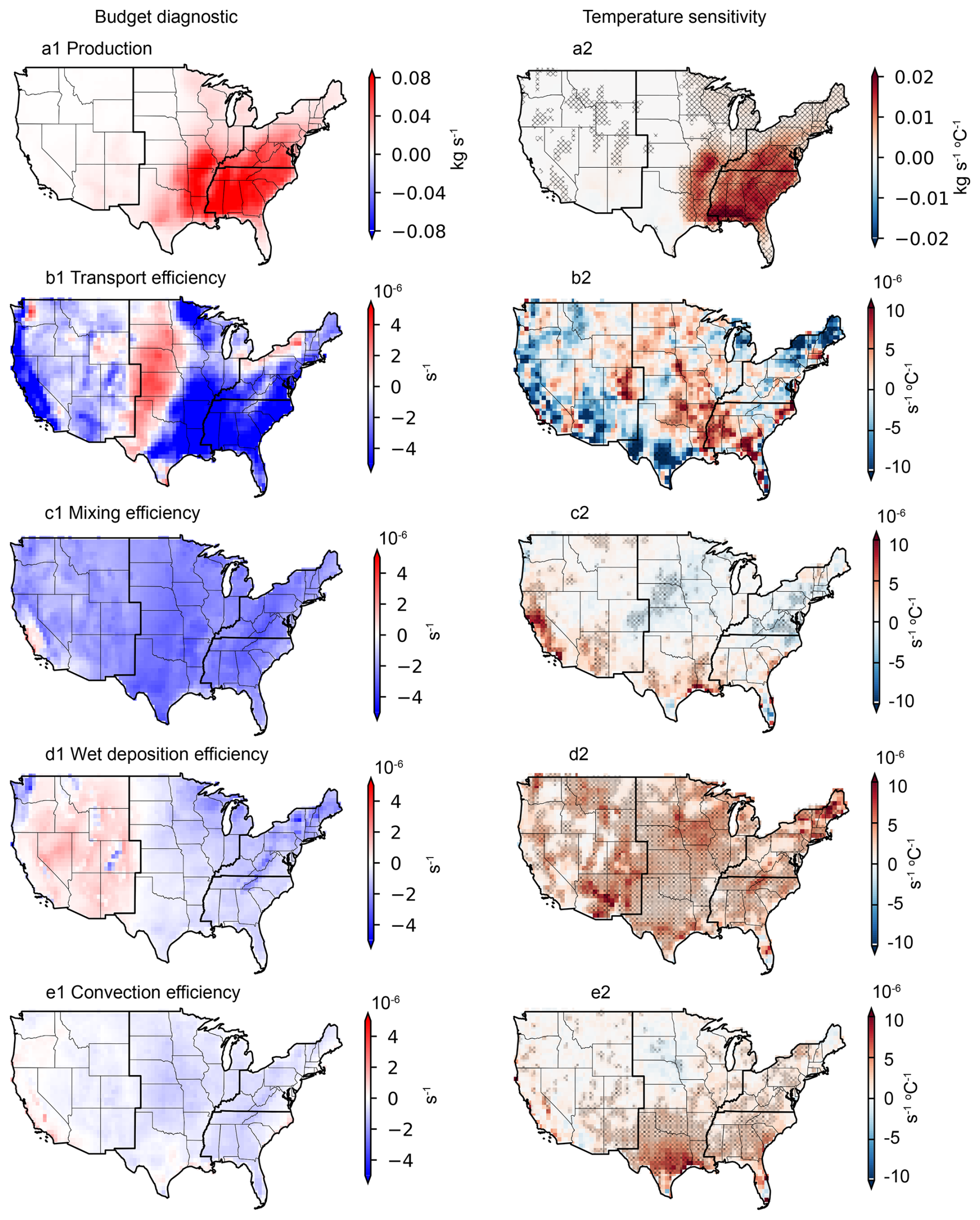
Figure 3 Budget diagnostics for aqueous-phase-formed isoprene SOA (ISOAAQ) and the temperature sensitivity of each process. Results are from the MAIN_HighRes case spanning 2000 to 2022. Stippling represents fitted temperature sensitivities with p-value < 0.05. Panels (a1)–(a2) show the Production budget diagnostic (a1) and its derived temperature sensitivity (a2). Other panels represent the average efficiencies (lefthand column) and corresponding temperature sensitivities (righthand column) for transport (b1, b2), mixing (c1, c2), wet deposition (d1, d2), and convection processes (e1, e2).

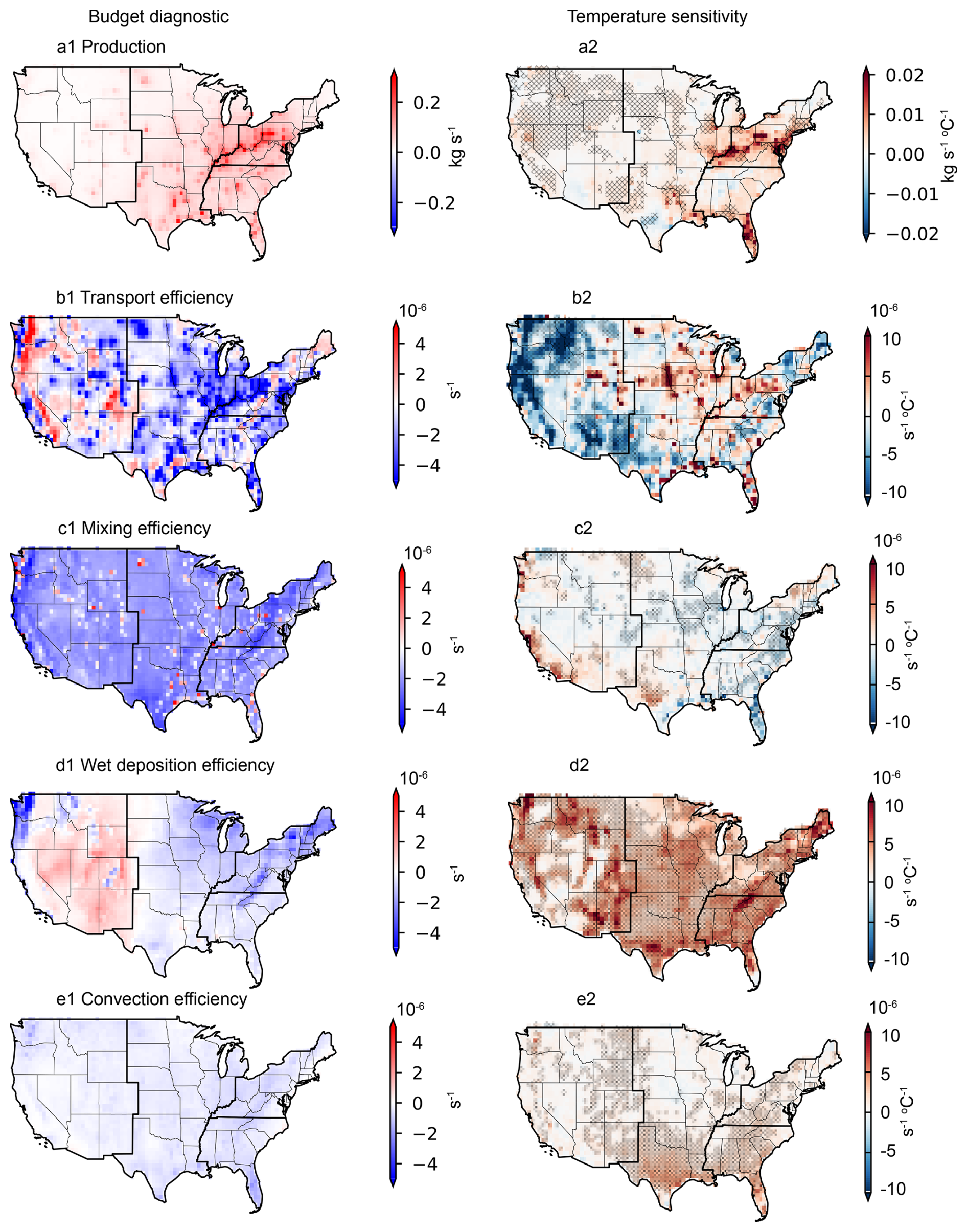
Figure 4 Same as Fig. 3 but for budget diagnostic and temperature sensitivity of sulfate.

The results show that chemical production leads to a positive mass change in ISOAAQ in the PBL across the CONUS from 2000 to 2022, with the largest increase occurring in the Southeast (Fig. 3a1). Horizontal and vertical transport generally reduce the PBL ISOAAQ mass in most regions, except for the central parts of the CONUS (Fig. 3a2). Mixing into the free troposphere also results in decreases in ISOAAQ mass throughout the CONUS. Wet deposition contributes to mass loss in the PBL in the Eastern US but leads to a mass increase in the Western US, likely due to re-evaporation of precipitation and particle resuspension processes. Cloud convection predominantly reduces ISOAAQ mass across most regions. Overall, chemical production is the primary driver of ISOAAQ mass increases, while transport emerges as the most efficient process for particle removal, followed by mixing, wet deposition, and cloud convection.

Figure 3a2–e2 illustrates the temperature sensitivity of the chemical production budget and the efficiencies of other processes. The chemical production of ISOAAQ shows a positive relationship with temperature across the CONUS, with the highest sensitivity in the Southeast, which could be related to increased isoprene emissions from forests and accelerated reaction rates. Because the chemical production process leads to an increase in mass, a positive production-temperature relationship indicates that as temperature increases, the mass increases, contributing to the positive temperature sensitivity of species, i.e., ISOAAQ in this case. In contrast, the temperature sensitivities of the other processes – transport, mixing, wet deposition, and convection – show a range of positive and negative values across the CONUS. For much of the CONUS, the temperature sensitivity of these processes is negative, and thus a negative relationship between the efficiency of these processes and temperature means that as temperature increases, efficiency increases, resulting in greater mass removal. The opposite is true for a positive efficiency-temperature relationship.

For example, although transport processes lead to decreased ISOAAQ mass in the Southeastern US, the temperature sensitivity of transport efficiency is positive in many grid cells in this region (Fig. 3b1–b2). This suggests that in warmer summers, transport efficiency could decline, allowing ISOAAQ to accumulate, thereby contributing to a positive temperature response. This reduced efficiency is likely linked to more stagnant, wind-free conditions typical of warmer weather in much of Southeastern US. The mixing efficiency shows less temperature dependence overall, with increases in the Northeast and decreases in the Southern US as temperatures rise (Fig. 3c1–c2). Wet deposition efficiency shows a positive correlation with temperature, which aligns with expectations of reduced precipitation and more frequent drought events in warmer summers, leading to decreased removal (Fig. 3d1–d2). Similarly, convection efficiency decreases with rising temperatures, as illustrated in Fig. 3e1–e2.

The budget analysis for sulfate reveals a pattern similar to that of ISOAAQ (Fig. 4), with a high production budget diagnostic observed in the eastern US. While most regions in the CONUS exhibit a positive temperature sensitivity for sulfate production, negative production-temperature relationships are identified in South Texas. This anomaly may be attributed to reduced aqueous-phase sulfate formation caused by decreased cloud cover at higher temperatures. The transport processes reduce sulfate concentrations in more polluted areas, such as the Eastern US, while increasing concentrations in less polluted regions, like the Western US. The temperature sensitivity of transport is generally opposite to its efficiency, indicating that transport efficiency decreases during warmer summers. Consistent with the findings for ISOAAQ, mixing efficiency exhibits a limited temperature dependence, while the removal efficiencies of wet deposition and cloud convection decline in warmer summers. This reduction in removal efficiency contributes to higher sulfate concentrations and a positive temperature sensitivity associated with these processes.

Figure 5 shows the time series of the temperature sensitivity for each process affecting ISOAAQ and sulfate over 5-year windows during 2000–2022. For comparison, the temperature sensitivities of ISOAAQ and sulfate concentrations are also shown. The results highlight that chemical production is the primary driver of both the signs and variability of ISOAAQ and sulfate sensitivities. Specifically, in the CONUS, as the production sensitivity decreased from 0.005 kg s⁻¹ °C⁻¹ to zero, the sensitivity of ISOAAQ concentration also decreased from 0.2 µg m⁻³ °C⁻¹ to zero, following similar interannual variations. At the regional scale, wet deposition and convection efficiencies are positively correlated with temperature, with a temperature sensitivity of 0.3 × 10⁻⁶ and 0.1 × 10⁻⁶ s⁻¹ °C⁻¹, respectively. This reflects reduced precipitation during warmer summers, leading to a positive response of air pollution to temperature. Conversely, mixing efficiency shows minimal temperature sensitivity, typically exhibiting a weak negative correlation with temperature, promoting dispersion of air pollution in the boundary layer during warmer summers. Transport efficiency demonstrates larger year-to-year variations compared to other removal processes. No significant temporal pattern is observed in the temperature sensitivities of transport, mixing, wet deposition, or convection efficiencies over the studied period.

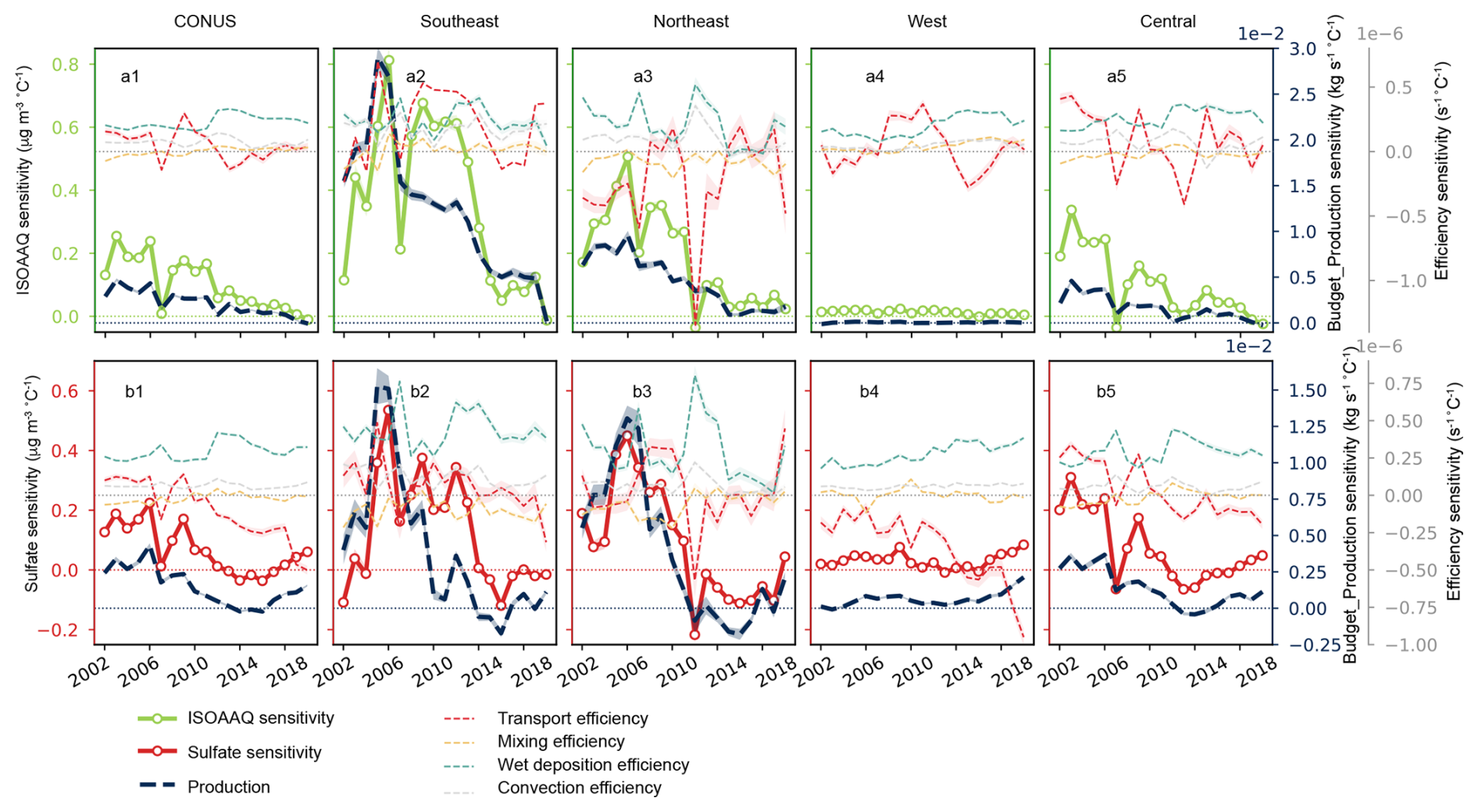
Figure 5 Regionally aggregated temperature sensitivities of the concentrations of isoprene SOA (ISOAAQ) and sulfate (left axes) and of the processes driving these concentrations (right axes). Shading represents the 95 % confidence interval. The top row shows the time series from ISOAAQ diagnostics for the contiguous US (a1), Southeastern US (a2), Northeastern US (a3), Western US (a4), and Central US (a5). The bottom row shows the results for sulfate in each region.

In the Southeast, the production sensitivity of ISOAAQ decreased by ∼ 40 % from 2005 to 2007 and continued declining after 2007. During the same period, the sensitivity of ISOAAQ concentration dropped by ∼ 75 % from 2005 to 2007 but then increased and stabilized at ∼ 0.6 µg m⁻³ °C⁻¹ between 2008 and 2014. This apparent inconsistency is likely due to variations in transport efficiency and its positive correlation with temperature during this period. During the 2005–2009 window, the temperature sensitivity of transport efficiency decreased from +2.6 × 10⁻⁷ to −6.4 × 10⁻⁸, and then increased to +3.6 × 10⁻⁷ during the 2006–2009 window. The negative sensitivity during 2005–2007 indicates that the transport efficiency increased with rising temperatures, reducing ISOAAQ concentration. The combined effects of decreased chemical production sensitivity and increased transport efficiency contributed to the sharp decline in ISOAAQ sensitivity during this period. From 2006 to 2014, while chemical production sensitivity continued to decline, transport efficiency sensitivity remained positive, indicating reduced transport efficiency with rising temperatures. This facilitated the buildup of ISOAAQ in the boundary layer, partially offsetting the impact of decreased chemical production sensitivity and resulting in stable ISOAAQ sensitivity during this period. A similar effect of reduced transport efficiency likely contributed to the increased ISOAAQ sensitivity observed in the Northeastern US during 2006–2014. These findings underscore that while ISOAAQ sensitivity is primarily driven by the temperature sensitivity of chemical production, fluctuations in the temperature sensitivity of transport efficiency also play a critical role in modulating the interannual variations of ISOAAQ sensitivity.

Similar to the ISOAAQ sensitivity, the decrease in the temperature sensitivity of sulfate concentration is primarily driven by the temperature response of chemical production, whereas the temperature response of transport efficiency plays an important role in interannual variations. The negative transport efficiency, which means higher transport efficiency in warmer summers, contributes to notable decreases in sulfate sensitivity. This impact is particularly evident during 2005–2009 in the Southeastern US and Central US (Fig. 5b2, b5) and 2010–2014 in the Northeastern US (Fig. 5b3). In summary, the budget diagnostic analysis reveals that chemical production is the dominant factor determining the decrease in ISOAAQ and sulfate sensitivities to temperature, which in turn drive the decrease in PM_2.5 sensitivity. Additionally, transport processes play a crucial role in shaping the interannual variations in ISOAAQ and sulfate sensitivities to temperature.

The temperature sensitivity of major processes contributing to POA concentration is shown in Fig. S19a1–a5. Unlike the other species considered here, POA is directly emitted from fire events, making the emission process the dominant factor driving POA sensitivity. Additionally, the temperature sensitivity of transport significantly influences the interannual variation in POA sensitivity, particularly in the Southeast and Northeast US. TSOA, formed from monoterpene oxidation, is an important component of biogenic SOA. We find that the temperature sensitivity of TSOA is approximately an order of magnitude lower than that of isoprene SOA, typically ranging from 0 to 0.2 µg m⁻³ °C⁻¹ in most regions in the CONUS (Fig. S14). As with ISOAAQ, chemical production dominates the variability in TSOA sensitivity, whereas transport sensitivity contributes to the variations in certain years (Fig. S19b1–b5).

As previously discussed, GEOS-Chem tends to underestimate the sulfate sensitivity (Figs. 1b1–b5, S6b1–b4). Shen et al. (2017) attributed this underestimate to the overly rapid decrease in cloud fraction with rising temperatures in GEOS-5 meteorological reanalysis data. This rapid reduction significantly decreases aqueous-phase sulfate production at higher temperatures, contributing to the underestimation of sulfate sensitivity in GEOS-Chem. Xie et al. (2019) noted that while cloud fraction representation in MERRA-2 has been substantially improved, cloud cover still decreases too quickly under drought conditions, which frequently occur with high temperatures in summer. As a result, aqueous-phase sulfate production decreases under dry conditions in the MERRA-2-driven GEOS-Chem, leading to lower sulfate concentrations than is observed from ground-based measurements. In the MAIN_HighRes case, using CAMD scaling factors slightly improves sulfate sensitivity simulations, but the results still fall short of observed values (Fig. 1).

Considering that the magnitude of aerosol sensitivity is determined by the chemical production process, we investigated the contribution of different sulfate formation mechanisms based on the production rates diagnostic in GEOS-Chem. There are three major sulfate production pathways in GEOS-Chem: (1) gas-phase SO₂ oxidation by hydroxyl radical (^•OH), (2) in-cloud SO₂ oxidation by H₂O₂, and (3) in-cloud SO₂ oxidation by O₃. The production rate and temperature sensitivity for each pathway in the MAIN_HighRes case are shown in Fig. S20. Gas-phase SO₂ oxidation is the dominant sulfate production mechanism, followed by aqueous-phase oxidation by H₂O₂ and O₃. Gas-phase production hotspots are scattered across the Eastern US, while aqueous-phase production is concentrated in the Northeastern US and Appalachian regions (Fig. S20a1–a3). Gas-phase production rates exhibit positive correlations with temperature, particularly in the Northeastern US. Conversely, aqueous-phase production rates negatively correlate with temperature across the CONUS, with the strongest negative correlations observed in the southern Appalachian region and Texas. As shown in Figs. S20b1–b5 and S6b2, the underestimation of sulfate sensitivity to temperature in the Appalachian region in the MAIN_HighRes case is likely due to a combination of low gas-phase production sensitivity and a strong negative temperature sensitivity of aqueous-phase production. Although MERRA-2 meteorological reanalysis data have improved the issue of rapid cloud coverage decline with temperature increases (Fig. S8), cloud cover in the Appalachian region and Texas remains relatively more sensitive to temperature changes than in other areas. This heightened sensitivity leads to the pronounced negative temperature sensitivity of aqueous-phase sulfate formation in these regions, contributing to the underestimate of sulfate sensitivity in the model.

Figure S20c1–c5 illustrates the time series of the temperature sensitivity of each sulfate production pathway during the studied period. The gas-phase production rate, highly sensitive to ambient SO₂ concentrations, exhibited a significant decline in temperature sensitivity from 2000 to 2014, driven by effective emission control measures. After 2014, the temperature sensitivity of the gas-phase production rate decreased by an order of magnitude, stabilizing at a negligible level of approximately ∼ 0.0005 kg⁻¹ s⁻¹ °C⁻¹. These changes in gas-phase sulfate production have been the primary drivers of sulfate concentration sensitivity over the past two decades. By contrast, no significant pattern was observed in the temperature sensitivity of aqueous-phase sulfate formation rates during this period.

3.5 Quantifying the contributions from individual processes

As previously mentioned, ground-based observations and machine learning data can provide information on the total derivative of air pollution with respect to temperature (${\mathrm{dPM}}_{\mathrm{2.5}}/\mathrm{d}T$, $\mathrm{dSOA}/\mathrm{d}T$, $\mathrm{dsulfate}/\mathrm{d}T$). Chemistry transport models such as GEOS-Chem are helpful for breaking down the total sensitivity and quantifying the contributions from the individual processes. Based on the simulations from the modified GEOS-Chem model, we further investigated the contributions from various temperature-sensitive processes in the chemical formation to the aerosol-temperature sensitivity. The production of ISOAAQ and sulfate, the primary source of the overall PM_2.5 sensitivity, were used as examples for the quantification (Fig. 6). Additional discussions were provided for TSOA formation. The temperature sensitivities of ISOAAQ, sulfate, and TSOA are expressed as:

$$\begin{array}{}\text{(1)}& {\displaystyle }\begin{array}{rl}{\displaystyle \frac{\mathrm{dISOAAQ}}{\mathrm{d}T}}& ={\displaystyle \frac{\partial \mathrm{ISOAAQ}}{\partial \mathrm{Isoprene}}}\times {\displaystyle \frac{\partial \mathrm{Isoprene}}{\partial T}}\\ & +{\displaystyle \frac{\partial \mathrm{ISOAAQ}}{\partial {\mathrm{SO}}_{\mathrm{4}}}}\times {\displaystyle \frac{\partial {\mathrm{SO}}_{\mathrm{4}}}{\partial T}}+\mathrm{\dots }\end{array}\text{(2)}& {\displaystyle }\begin{array}{rl}{\displaystyle \frac{{\mathrm{dSO}}_{\mathrm{4}}}{\mathrm{d}T}}& ={\displaystyle \frac{\partial {\mathrm{SO}}_{\mathrm{4}}}{\partial {\mathrm{SO}}_{\mathrm{2}}}}\times {\displaystyle \frac{\partial {\mathrm{SO}}_{\mathrm{2}}}{\partial T}}+{\displaystyle \frac{\partial {\mathrm{SO}}_{\mathrm{4}}}{\partial \mathrm{OH}}}\times {\displaystyle \frac{\partial \mathrm{OH}}{\partial T}}\\ & +{\displaystyle \frac{\partial {\mathrm{SO}}_{\mathrm{4}}}{\partial \mathrm{CLDFRC}}}\times {\displaystyle \frac{\partial \mathrm{CLDFRC}}{\partial T}}+\mathrm{\dots }\end{array}\text{(3)}& {\displaystyle }\begin{array}{rl}{\displaystyle \frac{\mathrm{dTSOA}}{\mathrm{d}T}}& ={\displaystyle \frac{\partial \mathrm{TSOA}}{\partial \mathrm{TSOG}}}\times {\displaystyle \frac{\partial \mathrm{TSOG}}{\partial T}}+{\displaystyle \frac{\partial \mathrm{TSOA}}{\partial \mathrm{MTP}}}\times {\displaystyle \frac{\partial \mathrm{MTP}}{\partial T}}\\ & +{\displaystyle \frac{\partial \mathrm{TSOA}}{\partial {\mathrm{NO}}_x}}\times {\displaystyle \frac{\partial {\mathrm{NO}}_x}{\partial T}}+{\displaystyle \frac{\partial \mathrm{TSOA}}{\partial \mathrm{OH}}}\times {\displaystyle \frac{\partial \mathrm{OH}}{\partial T}}+\mathrm{\dots }\end{array}\end{array}$$

The temperature dependence of the reaction rates was not included due to the lack of GEOS-Chem output. For sulfate, only gas-phase production was considered as it predominantly drives the magnitude and variability of the production sensitivity (Fig. S20). It is important to note that the partial derivatives were not calculated under the assumption that other factors remain constant, as this would require substantial computational resources. Instead, similar to the temperature sensitivity calculations, each term was determined as the slope of the linear regression line for detrended anomalies as a first-order estimate. We acknowledge that this method may introduce uncertainties in our results due to interdependencies among the variables, but our analysis indicates that this approximation can well capture the total temperature sensitivity and provide useful insights into contributions from different processes.

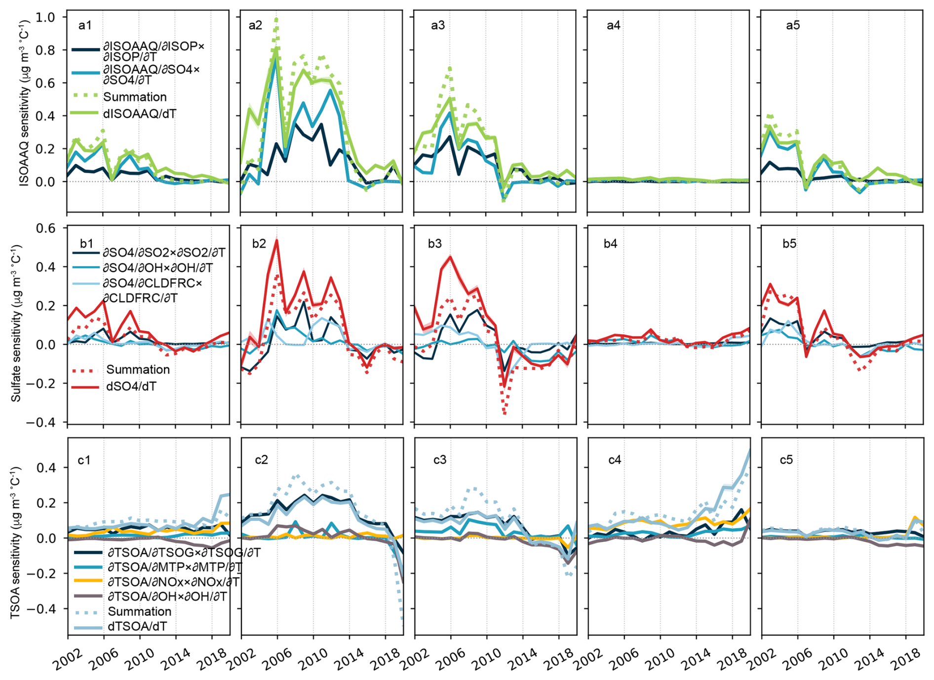
Figure 6 Contributions from major temperature-dependent processes to the overall temperature sensitivity of aqueous-phase formed isoprene SOA (ISOAAQ), sulfate, and monoterpene SOA (TSOA). Top row shows the results for ISOAAQ for the contiguous US (a1), Southeastern US (a2), Northeastern US (a3), Western US (a4), and Central US (a5). Middle row shows the results for sulfate in each region. Bottom rows show the results for TSOA in each region. Equations (1)–(3) provide detailed explanations of the terms.

The temperature sensitivity of ISOAAQ and relative contributions from the temperature dependence of isoprene and sulfate concentrations are shown in Fig. 6a1–a5. These two mediating processes exhibit similar long-term temporal pattern, with the sulfate-mediated temperature sensitivity being the most important factor influencing the magnitude and variability of the ISOAAQ-temperature relationship. It is important to note that these two processes are not entirely independent, and their combined contributions exceed the ISOAAQ sensitivity calculated directly from detrended anomalies of ISOAAQ concentration and temperature.

Figure S21a1–a5 shows the time series of the two processes contributing to the temperature dependence of ISOAAQ mediated by the temperature dependence of isoprene concentration: (1) $\frac{\partial \mathrm{Isoprene}}{\partial T}$, the sensitivity of isoprene concentration to temperature; and (2) $\frac{\partial \mathrm{ISOAAQ}}{\partial \mathrm{Isoprene}}$, the sensitivity of ISOAAQ concentration to isoprene concentration. Our results indicate that the variability of this term is mainly driven by  $\frac{\partial \mathrm{ISOAAQ}}{\partial \mathrm{Isoprene}}$, which has experienced a significant decrease in the Eastern and Central US over the time period. For example, in the Southeast, $\frac{\partial \mathrm{ISOAAQ}}{\partial \mathrm{Isoprene}}$ ranged from 0.10 to 0.61 µg m⁻³ ppb⁻¹ during 2000–2014, with an average of 0.38 µg m⁻³ ppb⁻¹, but dropped to −0.24 to 0.11 µg m⁻³ ppb⁻¹ (average: −0.03 µg m⁻³ ppb⁻¹) in recent years. Similarly, the average $\frac{\partial \mathrm{ISOAAQ}}{\partial \mathrm{Isoprene}}$ before 2016 was 0.30 µg m⁻³ ppb⁻¹ in the Northeast US and 0.31 µg m⁻³ ppb⁻¹ in the Central US, respectively. After 2016, these values decreased to 0.00 and 0.04 µg m⁻³ ppb⁻¹, respectively. The isoprene concentration positively correlates with temperature, and no significant temporal pattern was found during the study period.

Figure S21b1–b5 illustrates the temperature dependence of ISOAAQ mediated by the temperature dependence of sulfate aerosol. This relationship is quantified as the product of two terms: the sensitivity of sulfate to temperature change ($\frac{\partial {\mathrm{SO}}_{\mathrm{4}}}{\partial T}$) and the sensitivity of ISOAAQ concentration to sulfate concentration change ($\frac{\partial \mathrm{ISOAAQ}}{\partial {\mathrm{SO}}_{\mathrm{4}}})$. As previously discussed, $\frac{\partial {\mathrm{SO}}_{\mathrm{4}}}{\partial T}$ exhibits substantial variability and a clear decreasing pattern over the study period. Additionally, the average $\frac{\partial \mathrm{ISOAAQ}}{\partial {\mathrm{SO}}_{\mathrm{4}}}$ decreased by more than 60 % in the Eastern US from 2000–2014 to 2014–2022. Specifically, in the Southeast US, a unit increase in sulfate concentration could lead to a 1.34 µg m⁻³ increase in ISOAAQ concentration during 2000–2014, whereas this value decreased to 0.52 µg m⁻³ during 2014–2022. The reduced sensitivity of isoprene SOA formation to sulfate concentration can be attributed to changes in the relative abundance of organic and inorganic compounds. Over recent years, the increasing fraction of organic compounds could intensify the coating effect, which inhibits the uptake of IEPOX to form SOA. This may have led to a decline in the sensitivity of ISOAAQ to sulfate concentration. The product of $\frac{\partial \mathrm{ISOAAQ}}{\partial {\mathrm{SO}}_{\mathrm{4}}}$ and $\frac{\partial {\mathrm{SO}}_{\mathrm{4}}}{\partial T}$ generally follows variations in $\frac{\partial {\mathrm{SO}}_{\mathrm{4}}}{\partial T}$, emphasizing the critical role of sulfate-temperature sensitivity in shaping the overall temperature dependence of ISOAAQ.

The term $\frac{\partial \mathrm{ISOAAQ}}{\partial \mathrm{Isoprene}}$ reflects the conversion of isoprene to IEPOX and the subsequent uptake of IEPOX and SOA formation. These processes are related to factors that are closely linked to sulfate concentration, for instance, aerosol liquid water and the availability of proton donors and nucleophiles (Marais et al., 2016, 2017; Xu et al., 2015). Additionally, the coating effect considered in the modified GEOS-Chem model depends on the ratio between organic and inorganic aerosols, which is also influenced by sulfate concentration. Consequently, the $\frac{\partial \mathrm{ISOAAQ}}{\partial \mathrm{Isoprene}}$ is mediated by sulfate concentration, explaining its similar interannual variations and decreasing pattern alongside $\frac{\partial {\mathrm{SO}}_{\mathrm{4}}}{\partial T}$. Our findings suggest that sulfate concentration is the primary driver of the temperature sensitivity of aqueous-phase-formed isoprene SOA, underscoring the pivotal role of sulfate in regulating ISOAAQ temperature sensitivity.

Figure 6b1–b5 shows the contribution of the temperature sensitivity of SO₂, ^•OH radical, and cloud fraction to the overall sulfate sensitivity. The contribution of SO₂ can be represented as the product of the temperature response of SO₂ ($\frac{\partial {\mathrm{SO}}_{\mathrm{2}}}{\partial T}$) and the sensitivity of sulfate to changes in SO₂ concentration ($\frac{\partial {\mathrm{SO}}_{\mathrm{4}}}{\partial {\mathrm{SO}}_{\mathrm{2}}}$). As shown in Fig. S22a1–a5, $\frac{\partial {\mathrm{SO}}_{\mathrm{4}}}{\partial {\mathrm{SO}}_{\mathrm{2}}}$ shows no significant change over the study period. The average $\frac{\partial {\mathrm{SO}}_{\mathrm{4}}}{\partial {\mathrm{SO}}_{\mathrm{2}}}$ values during 2000–2014 were 1.7, 1.0, 0.2, and 2.1 µg m⁻³ ppb⁻¹ in the Southeast, Northeast, West, and Central US, respectively. During 2014–2022, the averages in these subregions changed to 1.8, 1.5, 0.2, and 1.6 µg m⁻³ ppb⁻¹, respectively. In contrast, $\frac{\partial {\mathrm{SO}}_{\mathrm{2}}}{\partial T}$ decreased from ∼ 0.1 ppb °C⁻¹ to near zero in most regions, except for the Western US, where wildfire emissions influenced SO₂ concentrations. This decline in the temperature sensitivity of SO₂ concentration drives the decrease in the first term in Eq. (2).

Similarly, the sulfate sensitivity mediated by the temperature response of the ^•OH can be calculated as the product of the sensitivity of the ^•OH concentration to temperature change ($\frac{\partial \mathrm{OH}}{\partial T}$) and the sensitivity of sulfate concentration to changes in ^•OH concentration ($\frac{\partial {\mathrm{SO}}_{\mathrm{4}}}{\partial \mathrm{OH}}$) (Fig. S22b1–b5). The temperature sensitivity of ^•OH exhibits an increasing tendency in the Eastern US and Central US but shows a decrease in the Western US. From 2000–2014 to 2014–2022, the average $\frac{\partial \mathrm{OH}}{\partial T}$ increased from −0.0009, 0.0006, 0.0041, and 0.0033 ppt °C⁻¹ to 0.003, 0.0045, 0.0014, and 0.0051 ppt °C⁻¹ in Southeast, Northeast, West, and Central US, respectively. The increased $\frac{\partial \mathrm{OH}}{\partial T}$ could be partially attributed to reductions in primary pollutant emissions, which lead to the accumulation of ^•OH in the atmosphere. Meanwhile, the sensitivity of sulfate concentration to ^•OH concentration shows a decreasing pattern from 2000 to 2014 and remains stable from 2014 to 2022 in most regions. Across the CONUS, the average $\frac{\partial {\mathrm{SO}}_{\mathrm{4}}}{\partial \mathrm{OH}}$ decreased from 3.5 µg m⁻³ ppt⁻¹ during 2000–2014 to −5.7 µg m⁻³ ppt⁻¹ during 2014–2022. Overall, the contribution of the temperature dependence of ^•OH to sulfate sensitivity decreases throughout the study period, although its magnitude remains small.

Figure S22c1–c5 illustrates the time series of two components of cloud fraction-mediated temperature sensitivity of sulfate. This term is calculated as the product of the temperature sensitivity of cloud fraction ($\frac{\partial \mathrm{CLDFRC}}{\partial T}$) and the sensitivity of sulfate to changes in cloud fraction ($\frac{\partial {\mathrm{SO}}_{\mathrm{4}}}{\partial \mathrm{CLDFRC}}$). As expected, $\frac{\partial \mathrm{CLDFRC}}{\partial T}$ is consistently negative in GEOS-Chem, indicating a decrease in cloud fraction with increasing temperature. However, $\frac{\partial {\mathrm{SO}}_{\mathrm{4}}}{\partial \mathrm{CLDFRC}}$ varies between positive and negative values. This variability reflects not only the influence of aqueous-phase formation but also processes related to precipitation and wet scavenging. Figure S20c1–c5 demonstrates that the aqueous-phase production rate decreases with rising temperatures during the study period. Despite this, the cloud-mediated process contributes positively to sulfate sensitivity in the earlier years, potentially driven by reduced wet scavenging during warmer summers with diminished cloud coverage.

All three processes significantly influence the magnitude of sulfate sensitivity. The SO₂-related process contributes more prominently to the Eastern and Central US, whereas in the Western US, the overall magnitude is primarily determined by the ^•OH-related process (Fig. 6b1–b5). The temperature dependence of SO₂ concentration largely determines the variability of sulfate sensitivity over time. During 2000–2010, the sum of contributions from these processes was lower than the overall sulfate sensitivity in the Eastern US, indicating that the other processes, including the temperature dependence of reaction rates and transport efficiency, may also play an essential role in driving the positive temperature sensitivity of sulfate. In conclusion, these findings demonstrate that the temperature sensitivity of sulfate is primarily governed by the temperature dependence of SO₂ concentration. The observed decrease in sulfate sensitivity after 2016 can be attributed to reductions in SO₂ concentrations during warmer summers.

The temperature sensitivity of SOA formed by monoterpene oxidation makes a non-negligible contribution to the overall SOA sensitivity, especially in the Southeast US (Fig. 1). To better understand this contribution, we decomposed the temperature sensitivity of TSOA into components mediated by TSOG (semi-volatile oxidation in the gas phase), which reflects the gas-particle phase partitioning, and by concentrations of monoterpenes, NO_x, and ^•OH (Figs. 6c1–c5 and S23). Our results reveal that phase partitioning plays a significant role in determining the magnitude of TSOA temperature sensitivity, particularly in the Southeast and Northeast US. Additionally, the temperature sensitivities of ^•OH and NO_x contribute to both the temporal pattern and interannual variations in TSOA sensitivity. This phenomenon is especially pronounced in the Western US, where NO_x concentrations are heavily influenced by wildfire emissions (Campbell et al., 2022), which have shown a consistent increase in recent years. The rising NO_x temperature sensitivity, combined with the temperature sensitivity of ^•OH, has driven a substantial increase in TSOA sensitivity in the West. The influence of NO_x is less significant in other regions. Zheng et al. (2023) suggested that the impact of anthropogenic NO_x on monoterpene SOA formation is missing from current models, highlighting the need for future studies to evaluate how this omission may affect simulations of temperature sensitivity.

To verify the robustness of the decomposition method, we performed a sensitivity analysis using multiple rolling temporal windows. In addition to the 5-year rolling windows shown in Fig. 6, we included results derived from 3-year rolling windows for isoprene SOA and sulfate (Fig. S24). This analysis serves as an uncertainty and robustness check, as shorter windows amplify sensitivity to interannual variability and potential detrending choices. Across both window lengths, the summed contributions from individual processes consistently reproduce the magnitude and variability of the total temperature sensitivity. The persistence of these patterns across different temporal windows provides confidence that the regression-based decomposition captures the dominant physical drivers despite unavoidable interdependencies among variables. Overall, the consistency of process contributions across rolling window lengths indicates that the decomposition is robust to temporal sampling and detrending assumptions.

Additionally, we performed a decomposition analysis for nitrate to investigate the mechanisms driving the model's predicted negative temperature sensitivity. We expressed particulate nitrate NO${}_{\mathrm{3}}^{-}$) as the product of total nitrate (TNO₃ = HNO₃ + NO${}_{\mathrm{3}}^{-}$) and the particle-phase fraction (f_p).

$$\left[{\mathrm{NO}}_{\mathrm{3}}^{-}\right]=\left[{\mathrm{TNO}}_{\mathrm{3}}\right]\times f_{\mathrm{p}}$$

The temperature sensitivity was then decomposed into two terms:

$$\begin{array}{}\text{(4)}& {\displaystyle \frac{\mathrm{d}\left[{\mathrm{NO}}_{\mathrm{3}}^{-}\right]}{\mathrm{d}T}}\approx f_{\mathrm{p}}\times {\displaystyle \frac{\mathrm{d}\left[{\mathrm{TNO}}_{\mathrm{3}}\right]}{\mathrm{d}T}}+\left[{\mathrm{TNO}}_{\mathrm{3}}\right]{\displaystyle \frac{\mathrm{d}{f}_{\mathrm{p}}}{\mathrm{d}T}}\end{array}$$

Production Driver $\frac{\mathrm{d}\left[{\mathrm{TNO}}_{\mathrm{3}}\right]}{\mathrm{d}T}$: Sensitivity mediated by changes in total nitrate (driven by NO_x emissions and oxidation).

Thermodynamic Driver $\frac{\mathrm{d}{f}_{\mathrm{p}}}{\mathrm{d}T}$: Sensitivity mediated by changes in the gas-particle partitioning fraction f_p.

Our analysis confirms that the thermodynamic driver is the dominant factor, as shown in Fig. S25. The model simulates a strong negative response of the partitioning fraction to temperature, which causes substantial volatilization of ammonium nitrate. This negative thermodynamic term overwhelms the production term, which is weakly positive, driven by slight increases in NO_x emissions or oxidation rates with temperature. This quantification highlights that the model's negative nitrate bias is largely due to the high sensitivity of the partitioning equilibrium to temperature.

4 Conclusions

Understanding the mechanisms driving the response of PM_2.5 and its components to rising temperatures is critical for improving future air quality and climate projections, given the complex interactions between aerosols and climate change. While previous studies have established observational correlations between aerosols and temperature and highlighted model biases, our study advances this field by comprehensively evaluating and improving the performance of the GEOS-Chem model in simulating the temperature sensitivity of PM_2.5 and its species across the contiguous United States. We further quantify the contributions of relevant processes to this sensitivity, thereby identifying the dominant drivers for both total PM_2.5 and its individual components. The baseline model significantly overestimated PM_2.5 temperature sensitivity, particularly in the Southeast and West US, driven by excessive contributions from biomass burning POA emissions and SOA formation processes, which increased with rising temperatures. Additionally, the model underestimated the temperature sensitivity of sulfate. To address these issues, targeted modifications were implemented, including adopting the GFED4 inventory for biomass burning emissions, incorporating the coating effects on the aqueous-phase isoprene SOA formation, and applying updated scaling factors for SO₂ and NO_x emissions from energy-generated units. These adjustments significantly reduced the discrepancies, aligning simulated results more closely with observations and machine-learning-derived datasets.

The GFED4 inventory proved effective in reproducing more reasonable temperature sensitivities of wildfire emissions and their increasing patterns. The default complex SOA scheme in GEOS-Chem overestimated SOA temperature sensitivity, especially in the southeastern US, primarily due to its overly strong dependence on sulfate concentrations. This led to an overestimation of isoprene SOA levels. Incorporating coating effects into the aqueous-phase isoprene SOA formation process addressed this issue effectively, aligning model results more closely with observations. Conversely, while the simple SOA scheme demonstrated reasonable performance in simulating overall SOA concentrations, it failed to capture the strong positive temperature sensitivity of SOA formation and its decreasing pattern observed in the US. This limitation highlights the necessity of incorporating improved formation mechanisms to accurately simulate the temperature dependence of air pollution, particularly for projecting future air quality under changing climatic conditions and for understanding climate-aerosol feedbacks.

The modified GEOS-Chem model successfully reproduced the magnitude and variability of PM_2.5 temperature sensitivity. Analysis of model outputs revealed that chemical production primarily determines the sign and long-term changes in temperature sensitivity for isoprene SOA and sulfate, which are key contributors to PM_2.5 sensitivity. However, transport processes play a critical role in shaping the interannual variability of temperature sensitivity. In addition, the temperature sensitivity of POA, a significant contributor to overall OA and PM_2.5 sensitivity, is predominantly influenced by wildfire emissions, with transport processes further modulating interannual variations. The temperature sensitivity of monoterpene SOA is driven by temperature-dependent phase partitioning and chemical production processes.

Improvements in sulfate sensitivity estimation were achieved by applying CAMD scaling factors to improve interannual variability in SO₂ emissions, but underestimation persisted in regions such as the Appalachian Mountains. These biases were attributed to an overly rapid decrease in cloud cover with temperature in the MERRA-2 meteorological data, which reduced aqueous-phase sulfate production. Regionally, gas-phase oxidation dominated sulfate temperature sensitivity during the study period, but its influence has declined and stabilized since 2014 as a result of emission control strategies. The response of aqueous-phase formation is insensitive to SO₂ emission change and shows no significant variations over the study period. The persistent underestimate of sulfate sensitivity in regions where aqueous-phase formation plays a critical role highlights the urgent need to refine our understanding and parameterization of cloud-temperature interactions in meteorological models, specifically for fair-weather cumulus clouds, which are challenging to capture in models. Improving these processes is essential for enhancing the accuracy of air quality and climate predictions.

We quantified the contributions from the temperature-dependence of isoprene and sulfate to ISOAAQ sensitivity. The sum of the temperature sensitivities mediated by these two processes reasonably matches the observed ISOAAQ sensitivity, despite their interdependence. Our results highlight a dominant role of sulfate sensitivity due to its influence on ISOAAQ formation through the aerosol liquid water content and coating thickness, which is determined by the relative abundance of organic and inorganic compounds. Given the important role of gas-phase production in modulating sulfate sensitivity, as indicated by our findings, we further quantified the contributions from the temperature response of precursors of the gas-phase reaction precursors (SO₂ and ^•OH) and the cloud fraction to sulfate temperature sensitivity. The long-term temporal pattern of the temperature sensitivity of sulfate is mainly driven by the decreasing response of SO₂ concentration to temperature as SO₂ emissions declined overall. The combined contributions of SO₂, ^•OH and cloud fraction adequately explain sulfate sensitivity after 2014. The remaining sensitivity during 2000–2014 is likely attributable to temperature-sensitive reaction rates. Our findings suggest that reductions in anthropogenic SO₂ emissions have decreased the temperature sensitivities of both sulfate and isoprene SOA, thereby reducing overall PM_2.5 temperature sensitivity. For monoterpene SOA, gas-particle phase partitioning plays a significant role in overall sensitivity, while its dependence on precursor concentrations including monoterpenes, ^•OH, and NO_x, collectively contributes to interannual variability.

There are several limitations to the present study. First, when using the budget diagnostics from GEOS-Chem simulations to quantify the contribution of each process, the partial derivatives were calculated in the same manner as total derivatives, without holding other variables constant, as required by the strict physical definition of partial derivatives. Although the results show acceptable agreement with total derivatives, it should be noted that potential interdependencies among different processes may exist. Second, due to the lack of available observational data to validate the mass changes associated with the relevant physical and chemical processes simulated by GEOS-Chem, the results should be interpreted with a reasonable degree of caution. Third, one dataset used to evaluate the performance of GEOS-Chem was the temperature sensitivity derived from ML models, which included GEOS-Chem estimates (REF_2019 case) as one of the input features. Although the incorporation of ground-based observations, satellite data, and simulations from other models was intended to reduce dependence on GEOS-Chem outputs, potential residual dependence in the model evaluation cannot be entirely ruled out, particularly for regions with sparse observations. Nevertheless, this limitation does not affect the conclusion regarding the improved performance of our modified model, as the evaluation also included PM_2.5 and its species-specific temperature sensitivities derived from observations. Furthermore, regarding the methodology for deriving temperature sensitivity, we used local measurements or simulations of PM_2.5 and temperature. We acknowledge that in regions where PM_2.5 is strongly influenced by long-range transport, this approach may introduce biases. However, the use of summer mean concentrations helps mitigate this issue in areas where air pollution is primarily driven by local sources.

An additional source of uncertainty concerns the treatment of POA volatility. Although a semi-volatile treatment of POA is generally recommended for applications focused on reproducing absolute OA burdens (Pai et al., 2020a), it has also been shown to introduce longer atmospheric residence times and enhanced low-tropospheric POA concentrations, reflecting uncertainties in volatility distributions, aging processes, and removal pathways. We acknowledge that disabling the semi-volatile POA option may affect simulated OA mass. However, process-based diagnostics indicate that the temperature sensitivity of POA is dominated by the temperature dependence of primary emissions, particularly wildfire emissions (Fig. S19). Consequently, the diagnosed POA temperature sensitivity is largely insensitive to the choice of POA volatility treatment. Moreover, oxidized POA is not included in the SOA mass in GEOS-Chem, such that enabling the semi-volatile POA option does not directly affect SOA formation pathways. The dominant drivers of OA and PM_2.5 temperature sensitivity in the eastern US – namely isoprene-derived SOA production and sulfate-mediated chemical processes – are therefore not expected to be significantly affected by this modeling choice.

Overall, this study establishes a robust framework for evaluating and improving the representation of air pollutant temperature sensitivity in chemistry transport models. These insights will contribute to more accurate predictions of future air quality under climate change scenarios and will provide valuable guidance for developing strategies to mitigate the health and environmental impacts of air pollution.