Aging of droplet size distribution in stratocumulus clouds: regimes of droplet size distribution evolution

The climatic impact of maritime stratocumulus clouds depends on the evolution of their droplet size distribution (DSD), yet the mechanisms controlling their variability during evaporation remain poorly constrained. Using large-eddy simulations coupled with a Lagrangian cloud model, we demonstrate that the DSD evolution follows two primary regimes: adiabatic growth and entrainment–descent. Within the latter, DSD evolution follows divergent pathways determined by the parcel's entrainment history: strong entrainment-driven dilution near the cloud top causes rapid broadening, whereas large-scale boundary-layer descent leads to gradual evaporation. Our Lagrangian analysis of the Damköhler number reveals that the commonly observed vertical transition from inhomogeneous to homogeneous mixing signatures does not necessarily reflect a change in the local mixing mechanism. Instead, it results from the vertical sorting of parcels with divergent histories. Parcels subject to strong entrainment retain inhomogeneous signatures throughout their descent, while those experiencing minimal dilution exhibit homogeneous-like characteristics regardless of altitude. This distinction helps resolve ambiguities in interpreting in situ observations where mixing history is often unknown. Finally, we propose a combined analytical–empirical formulation that captures the relative dispersion during both growth and evaporation.

1 Introduction

Maritime stratocumulus (Sc) clouds play a key role in Earth's climate by cooling the planet through the reflection of large amounts of incoming solar radiation (Chen et al., 2000; Siebesma et al., 2004; Wood, 2012). Stratocumulus-topped boundary layers (STBLs) are characterized by a Rayleigh-Bénard-type circulation, driven predominantly by longwave radiative cooling at the cloud top (e.g. Wood, 2012; Mellado, 2017). This circulation is characterized by broad, cloud-laden updrafts and narrow, nearly cloud-free downdrafts known as cloud holes (e.g. Krueger, 1993; Korolev and Mazin, 1993; Gerber et al., 2005). As droplets cycle through this dynamic environment, they undergo activation, condensational growth, entrainment-driven evaporation, and circulation-induced descent, leading to systematic changes in the droplet size distribution (DSD). The DSD fundamentally governs cloud optical properties (Considine and Curry, 1996; Pawlowska et al., 2006; Chandrakar et al., 2022) and precipitation initiation (Seifert and Beheng, 2006).

To capture the time-dependent transformation of cloud microphysics, we define “DSD aging” as the temporal evolution of its shape. Although this concept has previously been introduced in the context of precipitation initiation (Seifert and Beheng, 2006), we specifically use it here to describe the microphysical evolution of the DSD driven by condensation, evaporation, entrainment, and mixing. We characterize DSD aging using two key parameters: the arithmetic mean droplet radius (r_m=〈r〉) and the relative dispersion (d_r), defined as the ratio of the standard deviation to the mean radius. The relative dispersion d_r describes the relative width of the size distribution. It is a key determinant of both cloud optical properties and rain initiation (Liu and Daum, 2004; Liu et al., 2008; Wang et al., 2021), yet it is rarely predicted in conventional moment-based microphysical models. Therefore, understanding DSD aging within the STBL is essential for improving cloud–aerosol–precipitation interactions in climate models, as it links intricate DSD shapes to more predictable boundary layer dynamics.

Previous studies indicate that the correlation between d_r and mean droplet size varies with dominant microphysical processes and environmental conditions, often shifting between positive and negative across different stages of droplet evolution (Chandrakar et al., 2018; Lu et al., 2020; Luo et al., 2022). We note that some prior studies utilize the volume-mean radius ($r_{\mathrm{v}}=\langle r^{\mathrm{3}}{\rangle }^{\mathrm{1}/\mathrm{3}}$), which is weighted toward larger droplets (e.g. Chandrakar et al., 2018; Lu et al., 2020). While r_v≥r_m, both metrics generally capture similar evolutionary trends in this context. Focusing on r_m, specifically within an adiabatically ascending parcel, condensational growth leads to an increase in r_m while d_r decreases. This occurs because smaller droplets grow faster, causing the DSD to narrow (Yau and Rogers, 1996). This inverse relationship is well-characterized by existing analytical expressions (Liu et al., 2006).

However, during entrainment and mixing, the changes in r_m and d_r become more complex and less predictable. This complexity arises because entrainment is a non-adiabatic and intermittent process. The amount of free-tropospheric air that is entrained, the rate at which it mixes with cloudy air, and the timescale over which the mixture approaches thermodynamic equilibrium, all of which are critical for understanding how entrainment and mixing influence DSD shape, remain poorly constrained in both observations and models. In addition, the specific mixing scenario further complicates predictions. Under homogeneous mixing, r_m typically decreases and d_r increases as all droplets partially evaporate (Baker and Latham, 1979). In contrast, inhomogeneous mixing may leave both parameters largely unchanged while decreasing the droplet number concentration through the complete evaporation of some droplets (Baker and Latham, 1979; Baker et al., 1980; Lehmann et al., 2009). Even r_m can increase and d_r decrease in a “narrowing” mixing scenario as suggested in a recent study (Lim and Hoffmann, 2023). In situ measurements often reveal inhomogeneous mixing signatures near the cloud top and homogeneous characteristics below (Wang et al., 2009; Yum et al., 2015; Yeom et al., 2021). However, it remains unclear whether this reflects a true change in the physical mixing mechanism or results from other processes, such as dilution or the vertical sorting of parcels with different mixing histories. Therefore, to understand the spatiotemporal variability of d_r in stratocumulus clouds, it is essential to resolve how entrainment and mixing interact with the Lagrangian history of the droplets.

In this study, we employ the L³ model (Hoffmann et al., 2019; Hoffmann and Feingold, 2019; Lim and Hoffmann, 2023, 2024), a novel framework that combines large-eddy simulation (LES) with a linear eddy model (LEM) and a Lagrangian cloud model (LCM). The L³ model explicitly resolves subgrid-scale (SGS) supersaturation (S) fluctuations and turbulent mixing using the LEM, which mimics fine-scale turbulent stirring and scalar transport (Kerstein, 1988). The LCM tracks individual hydrometeors (e.g. Hoffmann et al., 2015), represented as computational particles that stand in for ensembles of real droplets or aerosols (Shima et al., 2009), thereby capturing detailed microphysical processes. This Lagrangian approach enables us to track individual particles along their trajectories through the STBL vertical circulation, capturing the evolving thermodynamic and microphysical conditions that govern droplet growth. In particular, it allows for a detailed quantification of how the DSD shape evolves along distinct pathways shaped by droplet activation, condensation, entrainment, mixing, and evaporation.

This paper is structured as follows. Section 2 presents the L³ model framework and simulation settings. Section 3 shows how the DSD shape parameters evolve in different regimes. In Sect. 4, we discuss a method to predict d_r in these regimes. Finally, we conclude our paper in Sect. 5. Parts of this study are based on the first author's dissertation (Lim, 2024), which has been extended with special attention to the impact of different mixing pathways (Sect. 3.3.3 and 3.4) and more general conclusions (Sect. 5).

2 Model and Simulations

2.1 The L³ model

We employ the novel L³ model (Hoffmann et al., 2019), built upon the System for Atmospheric Modeling (SAM), a nonhydrostatic, anelastic LES model (Khairoutdinov and Randall, 2003). Cloud microphysical processes are modeled using the LCM, employing individually simulated computational particles, i.e. LCM particles, where each particle represents a group of identical hydrometeors. Additionally, the linear eddy model (LEM), an explicit turbulence and mixing model (Kerstein, 1988; Krueger et al., 1997), is coupled with the LCM and LES to represent the unresolved effects of entrainment and mixing on droplet growth (Hoffmann et al., 2019; Hoffmann and Feingold, 2019; Lim and Hoffmann, 2023, 2024).

In the Lagrangian Cloud Model (LCM), condensational growth of droplets is driven by the supersaturation,

$$\begin{array}{}\text{(1)}& {\displaystyle }{\displaystyle }S=\overline{S}+S^{\prime },\end{array}$$

where the LES-resolved mean supersaturation is

$$\begin{array}{}\text{(2)}& {\displaystyle }{\displaystyle }\overline{S}={\displaystyle \frac{{\overline{q}}_{\mathrm{v}}}{q_{\mathrm{s}}(\overline{T},p)}}-\mathrm{1}.\end{array}$$

Here, ${\overline{q}}_{\mathrm{v}}$ is the LES-resolved water vapor mixing ratio, and q_s is the saturation vapor mixing ratio determined by the LES-resolved temperature $\overline{T}$ and pressure p. The fluctuation term S^′ represents the deviation from $\overline{S}$ and is tracked individually for each LCM particle, being updated continuously throughout its growth history. The LEM redistributes S^′ among the LCM particles by mimicking turbulent compression and folding based on the LES subgrid turbulence kinetic energy. Therefore, in the L³ model, droplet condensational growth is determined by both $\overline{S}$ and S^′, allowing for a realistic representation of different mixing scenarios during entrainment and mixing (Lim and Hoffmann, 2023, 2024). Moreover, the standard deviation of supersaturation, σ_S, defined as the standard deviation of $S=\overline{S}+S^{\prime }$, is inherently resolved by the L³ model. Further details on the L³ framework can be found in Hoffmann et al. (2019).

2.2 Simulation Setup

A maritime nocturnal Sc cloud is simulated based on the Second Dynamics and Chemistry of Marine Stratocumulus Field Study (DYCOMS-II) campaign (Stevens et al., 2003), with fixed surface fluxes, subsidence, and a simple parameterization for longwave radiative cooling (Ackerman et al., 2009). The model domain is $\mathrm{3.2}\mathrm{km}\times \mathrm{3.2}\mathrm{km}\times \mathrm{2.56}\mathrm{km}$ in x, y, and z directions. We use a grid spacing of $\mathrm{10}\mathrm{m}\times \mathrm{10}\mathrm{m}\times \mathrm{5}\mathrm{m}$ to resolve the energy-containing eddies and the sharp thermodynamic gradients across the entrainment interface layer. Unresolved scalar inhomogeneity and turbulent mixing that control droplet response are represented by the coupled LEM (Hoffmann et al., 2019), which redistributes the particle-level supersaturation fluctuation S^′ at an effective vertical resolution of $\mathrm{\Delta }{z}_{\text{LEM}}=\mathrm{\Delta }{z}_{\text{LES}}/n_{\mathrm{p}}\approx \mathrm{5}\mathrm{cm}$ (see below). The model time step δt=0.5 s, and the total model integration time is 5 h. The results are analyzed only for the last 2 h of the simulation.

The LCM particles, each representing the same number of hydrometeors, are initialized as sea-salt particles with dry radii randomly chosen from a log-normal distribution (geometric mean radius of r_{m, a}=80 nm, geometric standard deviation σ_r=1.4). Initial aerosol number concentrations of N_a=50, 100, and 200 cm⁻³ are considered, named N50, N100, and N200, respectively. Results are discussed mainly for the N100 case unless otherwise stated. Note that droplet sedimentation and collision–coalescence processes are not considered, as we focus on the evolution of the DSD shape in non-drizzling stratocumulus. Given the absence of drizzle, the maximum droplet radii are approximately 15, 12, and 9 µm for the N50, N100, and N200 cases, respectively. For droplets in the 5–15 µm range, terminal fall speeds are 𝒪 (1 cm s⁻¹) (Yau and Rogers, 1996), which is negligible compared to typical turbulent vertical-velocity fluctuations near cloud top (e.g. σ_w is $\mathcal{O}\left({\mathrm{10}}^{-\mathrm{1}}\mathrm{m}{\mathrm{s}}^{-\mathrm{1}}\right)$; Wood, 2012). However, neglecting sedimentation may slightly alter droplet residence times and hence microphysical exposure near cloud top.

The LEM further complements the high resolution of the LES. In the L³ model, the vertical LES grid spacing (Δz_LES) and the number of LCM particles per grid box (n_p) jointly determine the resolution of the LEM, defined as $\mathrm{\Delta }{z}_{\text{LEM}}=\mathrm{\Delta }{z}_{\text{LES}}/n_{\mathrm{p}}$. In this simulation, we initialize 100 LCM particles per grid box, resulting in a Δz_LEM of approximately 5 cm, which allows the model to represent fine-scale scalar inhomogeneity relevant for inhomogeneous mixing in stratocumulus within the L³ framework (Hoffmann and Feingold, 2019).

2.3 Lagrangian Particle Tracking

To explicitly resolve the microphysical histories of individual droplets, we implemented a Lagrangian particle-tracking algorithm within the L³ model. Each LCM particle is assigned a unique identifier (ID) upon initialization, which is preserved throughout its lifecycle. For this study, we tracked 400 particles. At initialization, four distinct and equidistantly spaced vertical columns were selected across the domain. Within each column, one particle was randomly chosen from each of the lowest 100 vertical grid boxes, yielding 100 tracked particles per column. To manage data volume and focus exclusively on in-cloud evolution, we applied a conditional recording scheme: data were recorded only when a flagged particle resided within a grid box classified as cloudy ($q_{\mathrm{c}}\ge \mathrm{0.01}\mathrm{g}{\mathrm{kg}}^{-\mathrm{1}}$). We used the first 3 h as a spin-up period, during which the flagged particles were dispersed by boundary-layer turbulence and became nearly well mixed within the boundary layer. Particle output was then enabled, and the final 2 h are used for analysis (Sect. 2.2).

These tracked particles function as “virtual observers”, although they remain microphysically active, undergoing condensation and evaporation indistinguishable from the standard LCM particles. At each time step, they sample the local thermodynamic conditions and record the bulk microphysical statistics of the droplet ensemble within their resident grid cell. Since particles typically undergo multiple cycles of entrainment and detrainment driven by turbulent vertical circulations, they often re-enter the cloud layer several times. Consequently, the effective number of in-cloud records is larger than the number of tracked LCM particles.

The recorded dataset includes each particle's Lagrangian state vector (unique ID, radius r, multiplicity, supersaturation fluctuation S^′, three-dimensional velocity components, and position) together with the co-located Eulerian state variables, including pressure p, turbulent kinetic energy dissipation rate ε, LES gridbox mean supersaturation $\overline{S}$, temperature T, and water vapor mixing ratio q_v. Additionally, properties derived from the full droplet population within the grid box, including q_c, cloud droplet number concentration N_c, supersaturation standard deviation σ_S, r_m, and d_r, were calculated and stored alongside the particle data. This approach ensures that the dataset captures the complete microphysical context of droplets, specifically during their residence in the cloud, filtering out the dry aerosol phase.

The resulting trajectories are recorded at a sampling interval equivalent to the model timestep (δt=0.5 s). To mitigate the high-frequency noise inherent to Lagrangian trajectories in turbulent flows, these properties were smoothed using a Gaussian kernel filter (Virtanen et al., 2020) with a window size of 10 s during post-processing.

3 Results

3.1 Dynamical and Mixing Characteristics of the STBL

We begin by characterizing the dynamical and mixing structure of the STBL. Figure 1a shows the mean vertical profile of two moist-adiabatically conserved variables: total water mixing ratio (q_t) and liquid water potential temperature (θ_l). The STBL consists of a well-mixed layer, characterized by high q_t and low θ_l, the free troposphere with low q_t and high θ_l, and an entrainment interface layer (EIL) in between. The EIL is characterized by sharp gradients in both moisture and temperature, typically within a few tens of meters. It represents the transition zone where turbulent eddies from the boundary layer mix with overlying dry and warm free-tropospheric air. Based on the sharp contrast in q_t and θ_l between the boundary layer and the free troposphere, we adopt a mixing fraction,

$$\begin{array}{}\text{(3)}& {\displaystyle }{\displaystyle }\mathit{\chi }={\displaystyle \frac{(q_{\mathrm{t}}-q_{\text{t,bl}})}{(q_{\text{t,ft}}-q_{\text{t,bl}})}},\end{array}$$

which represents the fraction of free-tropospheric air mixed with boundary-layer air (Yang et al., 2016; Lu et al., 2018b). While calculating χ using θ_l yields results highly correlated with those based on q_t, we select q_t as the conserved variable because it exhibits a more constant profile in the free troposphere (Fig. 1a), making the choice of representative free-troposphere value easier.

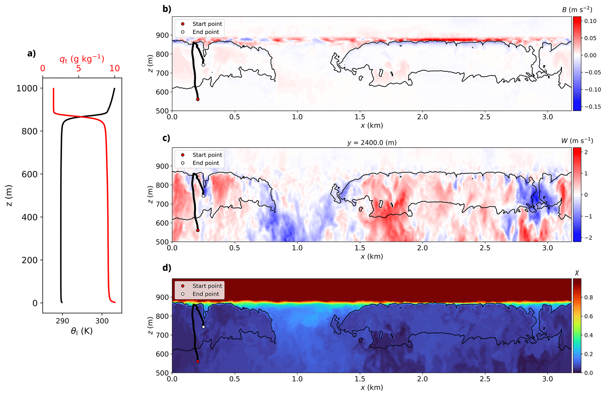
Figure 1 (a) Vertical profiles of q_t (red solid line) and θ_l (black solid line). Vertical cross-sections of (b) buoyancy B, (c) vertical velocity W, and (d) mixing fraction χ at y=2400 m, presented as a snapshot at a simulation time of t=13 320 s. In panels (b–d), the Lagrangian trajectory of a selected particle is overlaid as a thick black line, tracing its path from the entry point (red dot at t=12 298.5 s) to its current position (white dot at t=13 320 s). The thin black solid lines indicate where the cloud water mixing ratio $q_{\mathrm{c}}=\mathrm{0.01}\mathrm{g}{\mathrm{kg}}^{-\mathrm{1}}$.

In this simulation, the reference values q_t,ft and q_t,bl are set to their initial values of 1.5 and 9.5 g kg⁻¹, respectively, which remain nearly constant throughout the simulation. Note that turbulent fluctuations can cause local parcels to exhibit q_t values exceeding the domain-averaged q_t,bl, resulting in slightly negative χ values (accounting for ∼0.02 % of the total data; Fig. 2). These minor deviations reflect the natural physical variability within the boundary layer reservoir.

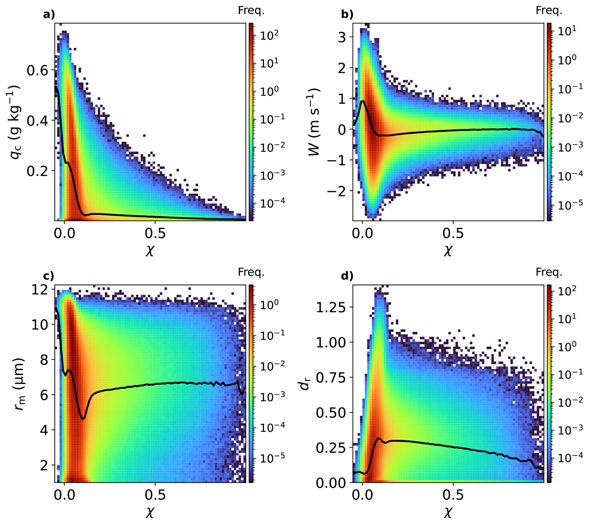
Figure 2 Two-dimensional density histograms of χ vs. (a) q_c, (b) W, (c) r_m, and (d) d_r, with black solid lines indicating the mean of each variable in bins of χ.

At the top of the STBL, stable stratification inhibits mixing between the boundary layer and the free troposphere. Consequently, χ is also strongly stratified (Fig. 1d), with the most rapid change confined to the EIL, identifying this region as the primary site of entrainment and mixing. The cloud top and EIL are persistently negatively buoyant (Fig. 1b), where the buoyancy is defined by

$$\begin{array}{}\text{(4)}& {\displaystyle }{\displaystyle }B=g\left({\displaystyle \frac{{\mathit{\theta }}_{\mathrm{v}}-{\overline{\mathit{\theta }}}_{\mathrm{v}}}{{\overline{\mathit{\theta }}}_{\mathrm{v}}}}\right)\end{array}$$

where g is the gravitational acceleration, and θ_v and ${\overline{\mathit{\theta }}}_{\mathrm{v}}$ are the local and horizontally averaged virtual potential temperatures, respectively. The negative B arises from evaporative cooling during entrainment and longwave radiative cooling (Stevens, 2002; Wood, 2012).

High values of χ are rarely observed within the cloud interior. However, localized pockets of enhanced χ can appear within the boundary layer, particularly near cloud holes and in descending branches of the STBL vertical circulation ($W<\mathrm{0}\mathrm{m}{\mathrm{s}}^{-\mathrm{1}}$, Fig. 1c). For example, at x=0.2 km and x=3 km, cloud holes coincide with downdrafts and elevated χ, possibly indicating the accumulation of previously entrained dry air.

While χ can highlight regions influenced by entrainment, its relationship with microphysical variables such as r_m and d_r is not straightforward. To explore this quantitatively, Fig. 2 illustrates the relationships between various variables and χ. q_c is negatively correlated with χ, with high q_c ($>\mathrm{0.5}\mathrm{g}{\mathrm{kg}}^{-\mathrm{1}}$) occurring only in regions with very low χ (<0.1), corresponding to undiluted, nearly adiabatic cloud interiors. Notably, all panels show a dense cluster around χ<0.1, suggesting a prevalence of nearly adiabatic cloud interior during both ascent and descent (Fig. 2b). High values of χ are associated with $-\mathrm{1}\mathrm{m}{\mathrm{s}}^{-\mathrm{1}}<W<\mathrm{1}\mathrm{m}{\mathrm{s}}^{-\mathrm{1}}$, a range typically found in regions experiencing entrainment and mixing at the cloud top under near-neutral conditions.

Figures 2c and d show that r_m tends to decrease and d_r tends to increase with increasing χ in regions that remain nearly adiabatic (χ<0.1). However, when χ>0.1, the mean values flatten out, and the relationship becomes less clear: neither r_m nor d_r shows a strong or consistent dependence on χ. This suggests that while χ may correlate with microphysical variability in undiluted cloud regions, it alone cannot explain the droplet size evolution in environments influenced by entrainment and mixing. Therefore, to gain a more comprehensive understanding of the evolution of r_m and d_r, especially under the influence of entrainment and mixing, it is essential to consider the full growth history of individual droplets.

To illustrate this approach, Figs. 1 and 3 show an example particle trajectory that captures a representative pathway within the STBL vertical circulation. Droplets along this path undergo four key microphysical stages: (i) activation near the cloud base, (ii) condensational growth in updrafts, (iii) entrainment and mixing at the cloud top, and (iv) descent, evaporation, and deactivation. These stages leave clear imprints on the evolution of r_m and d_r. While both r_m and q_c generally increase with height in cloudy updrafts, a sharp decrease occurs near cloud holes (Fig. 3a and b), reflecting the effects of mixing and evaporation. In contrast, d_r shows a more complex distribution: it is typically lower inside clouds but increases near cloud top and cloud-hole boundaries (Fig. 3c), resembling the spatial structure of χ (Fig. 1d). In the following sections, we examine how particle histories shape distinct DSD aging regimes and control the evolution of r_m and d_r.

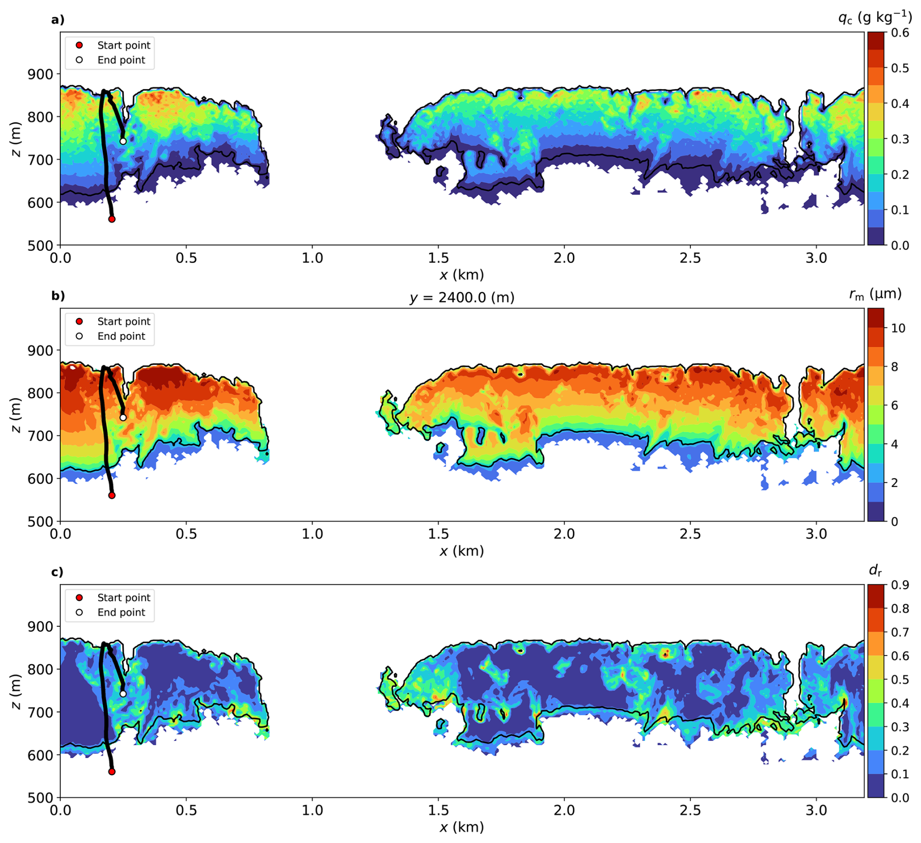
Figure 3 Vertical cross-sections of (a) q_c, (b) r_m, and (c) d_r at y=2400 m, presented as a snapshot at a simulation time of t=13 320 s. The thick black line traces the Lagrangian history of a selected droplet, ending at its current position (white dot) at this instant and extending backward in time to its cloud entry point (red dot). The thin black lines in each panel indicate the cloud boundary defined by a mixing ratio of $q_{\mathrm{c}}=\mathrm{0.01}\mathrm{g}{\mathrm{kg}}^{-\mathrm{1}}$.

3.2 Droplet Evolution Pathways in the r_m–d_r Phase Space

To further understand the evolution of r_m and d_r, we analyze the droplet evolution in the r_m–d_r phase space. Figure 4a shows the frequency distribution of the r_m–d_r phase space obtained from three-dimensional model output, where r_m and d_r are estimated from cloud droplets with radii >1 µm only. Overall, the range of d_r is inversely proportional to r_m, with d_r=1.0 at r_m=3 µm and d_r→0 for r_m=12 µm. The high-frequency pattern visible in Fig. 4a is divided into two distinct parts, which can be constrained by S (Fig. 5). We define these as the “growth pathway” characterized by low d_r for S≥0 and hence condensational growth (Fig. 5c and d), and the “evaporation pathway” characterized by high d_r for S<0 and hence evaporation (Fig. 5e and f). Thus, we expect a quasi-loop structure of droplet evolution from the growth pathway to the evaporation pathway. Figure 4b shows the LCM particle trajectories in this phase space, with black and green markers indicating the start and end points, respectively, and the corresponding frequency distribution in Fig. 4c. Note that the high-density patterns resemble the two pathways identified in the model output frequency distribution (Fig. 4a). In this analysis, we treat each continuous in-cloud segment of a particle trajectory as an independent trajectory, as a single particle can enter the cloud multiple times. This results in a total of 384 trajectory segments. We confirm that the qualitative features of Fig. 4 and other analyses presented later in this study (e.g. Fig. 5) remain unchanged when using subsets of 100, 200, or 400 trajectories, indicating that the results are robust with respect to sample size throughout the analysis.

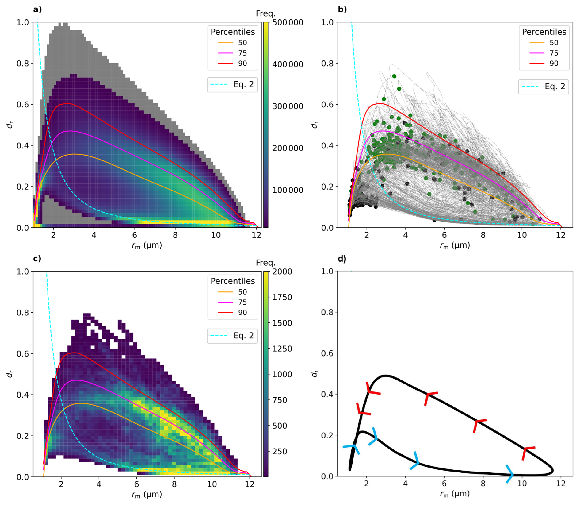
Figure 4 (a) Two-dimensional frequency histogram in r_m and d_r phase space. (b) Corresponding droplet evolution pathways (gray dotted lines) with start/end points in black/green. (c) The corresponding frequency distribution of droplet evolution pathways. (d) Conceptual schematic summarizing the composite evolution loop, constructed from the most frequently observed trajectory patterns in the r_m–d_r phase space. Blue and red arrows represent the dominant directions of growing and decaying pathways, respectively, based on the Lagrangian trajectory. In each panel, 50th, 75th, and 90th percentiles at each r_m value and Eq. (5) are indicated as solid lines in orange, magenta, red, and cyan, respectively. In panel (a), the gray-shaded regions indicate areas where the sample count is below 10 000, which are masked for statistical robustness.

The growth pathway can be described by

$$\begin{array}{}\text{(5)}& {\displaystyle }{\displaystyle }{d}_{\mathrm{r}}=d_{\text{r, 0}}{\displaystyle \frac{r_{\text{m, 0}}^{\mathrm{2}}}{r_{\mathrm{m}}^{\mathrm{2}}}},\end{array}$$

following the analytic solution proposed by Liu et al. (2006), where d_{r, 0} and r_{m, 0} denote the boundary values. Here, we use d_{r, 0}=0.01 and r_{m, 0}=12 µm to show Eq. (5) as a cyan dashed line in Fig. 4a and b.

While Eq. (5) effectively captures the growth pathway, it fails to describe the evaporation pathway (Fig. A1). To approximate the latter, we utilize percentile-based diagnostics, where the 50th, 75th, and 90th percentiles of d_r at each r_m bin provide a reasonable empirical representation of the evaporation pathway (Fig. 4a–c), exhibiting an inverse trend between d_r and r_m. In analogy to Eq. (5), the fitted function is given as

$$\begin{array}{}\text{(6)}& {\displaystyle }{\displaystyle }{d}_{\mathrm{r}}=d_{\text{r,max}}\left(\mathrm{1}-{\displaystyle \frac{r_{\mathrm{m}}^{\mathrm{2}}}{r_{\text{m,max}}^{\mathrm{2}}}}\right),\end{array}$$

where r_m,max and d_r,max denote the maximum values of r_m and d_r, respectively. Each percentile line (p50, p75, and p90) can be represented by a distinct d_r,max value for the same r_m (e.g. Fig. 4a). For instance, d_r approaches zero as r_m approaches r_m,max, whereas d_r,max typically occurs at much smaller droplet sizes (e.g. r_m<3 µm), well below r_m,max. A detailed discussion on this empirical formulation is provided in Sect. 4.

3.3 Different Regimes of Droplet Evolution Pathways

In the previous section, we showed that droplet evolution pathways diverge depending on whether droplets grow or decay. To better characterize these differences, we analyze the r_m–d_r phase space in terms of the sign of the correlation between $\mathrm{d}{d}_{\mathrm{r}}/\mathrm{d}t$ and $\mathrm{d}{r}_{\mathrm{m}}/\mathrm{d}t$. This analysis uses the particle trajectories shown in Fig. 4b and c.

As already indicated above, the resulting patterns are closely tied to the supersaturation S. As shown in Fig. 5a and b, the phase space structure under all S conditions can be decomposed into two dominant subsets based on S≥0 and S<0 (second and third rows). While the droplet life cycle is a continuous process, we can classify it into four distinct regimes, each characterized by a dominant set of microphysical processes: A (activation) and B (adiabatic growth) for S≥0, and C (entrainment and descent) and D (deactivation) for S<0, each of which corresponds to a dominant microphysical process. Although precipitation is another key process in DSD evolution, we focus on condensational growth and evaporation, examining phase-space-averaged microphysical and environmental properties across the four regimes (Figs. 6 and 7).

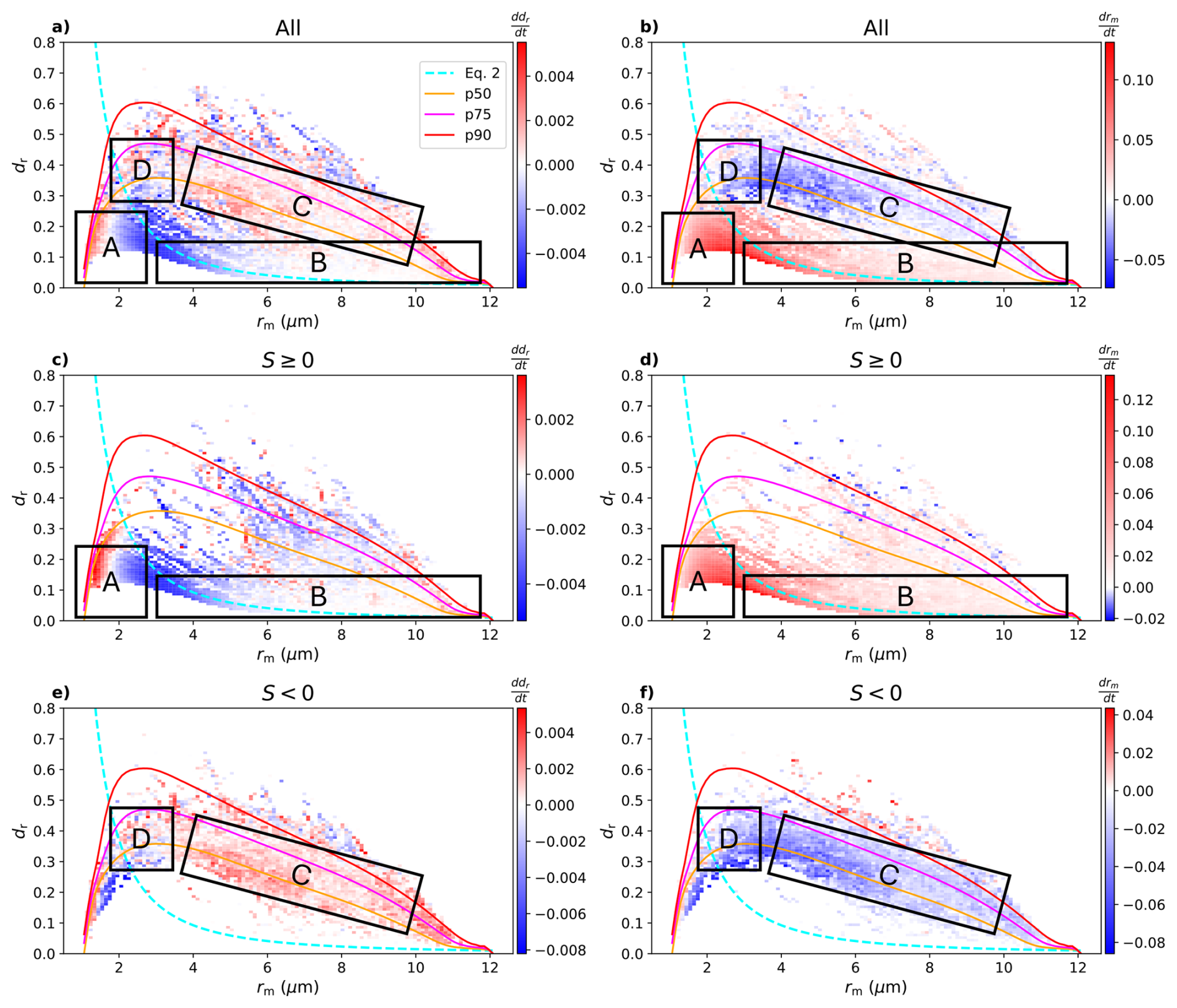
Figure 5 Two-dimensional binned mean values of the rates of change, $\mathrm{d}{d}_{\mathrm{r}}/\mathrm{d}t$ (first column) and $\mathrm{d}{r}_{\mathrm{m}}/\mathrm{d}t$ (second column), in the r_m–d_r phase space for all conditions (first row), S≥0 (second row), and S<0 (third row). In each panel, the 50th, 75th, and 90th percentile values (p50, p75, p90), and Eq. (5) from Fig. 4 are indicated by solid lines in orange, magenta, red, and cyan, respectively. Each panel shows 2D binned mean values of $\mathrm{d}{d}_{\mathrm{r}}/\mathrm{d}t$ and $\mathrm{d}{r}_{\mathrm{m}}/\mathrm{d}t$ in the r_m–d_r phase space, based on Lagrangian trajectories smoothed with a Gaussian kernel (window =10 s) and averaged over time.

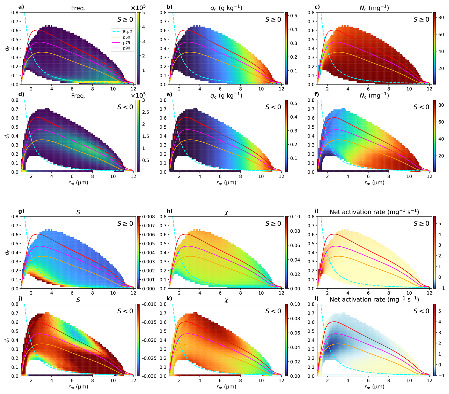
Figure 6 Two-dimensional binned mean values of cloud properties in the r_m and d_r phase space for S≥0 (first and third row) and S<0 (second and fourth row). (a) and (d) show the frequency distributions, (b) and (e) show cloud water mixing ratio (q_c), (c) and (f) show cloud droplet number concentration (N_c), (g) and (j) show the mean supersaturation (S), (h) and (k) show mixing fraction (χ) and (i) and (l) show net activation rate (activation rate – deactivation rate). In each panel, the 50th, 75th, and 90th percentile values (p50, p75, p90), and Eq. (5) from Fig. 4 are indicated by solid lines in orange, magenta, red, and cyan, respectively. Values represent bin-averaged means from 3D simulation results during the final 2 h of simulation, mapped onto the r_m–d_r phase space.

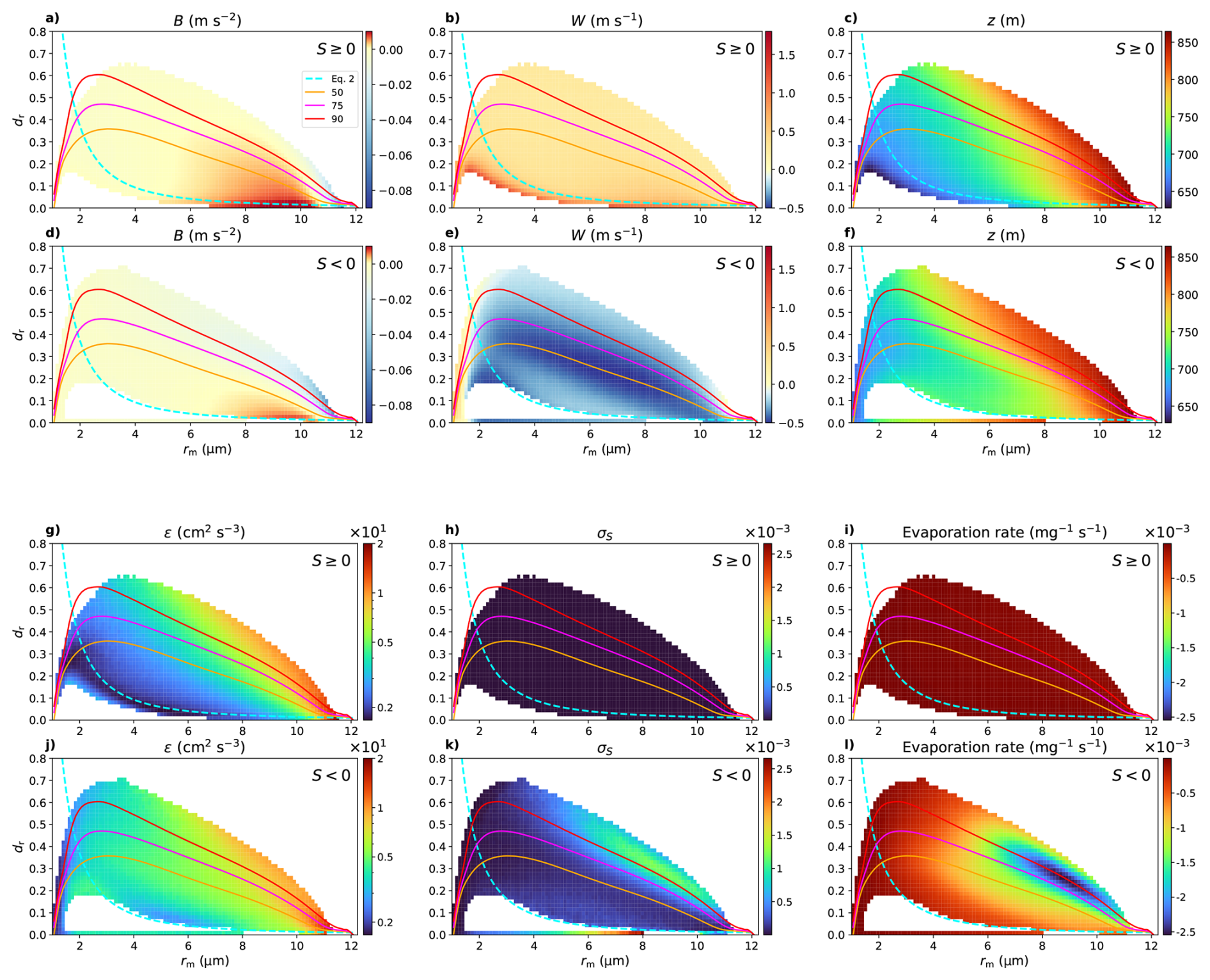
Figure 7 Two-dimensional binned mean values of cloud properties in the r_m and d_r phase space for S≥0 (first and third row) and S<0 (second and fourth row). (a) and (d) show buoyancy (B), (b) and (e) show vertical velocity (W), (c) and (f) show height (z), (g) and (j) show kinetic dissipation rate (ε), (h) and (k) show supersaturation fluctuation (σ_S) and (i) and (l) show the evaporation rate. In each panel, the 50th, 75th, and 90th percentile values (p50, p75, p90), and Eq. (5) from Fig. 4 are indicated by solid lines in orange, magenta, red, and cyan, respectively. Values represent bin-averaged means from 3D simulation results during the final 2 h of simulation, mapped onto the r_m–d_r phase space.

3.3.1 Activation Regime (S≥0)

In the activation regime, the $\mathrm{d}{r}_{\mathrm{m}}/\mathrm{d}t$–$\mathrm{d}{d}_{\mathrm{r}}/\mathrm{d}t$ correlation is primarily positive (region A in Fig. 5c and d), especially when r_m<2 µm. This regime is associated with droplet activation occurring in updrafts (Fig. 7b) near the cloud base (Fig. 7c), as indicated by high net activation rates (Fig. 6i). The corresponding increase in droplet number concentration (Fig. 6c) marks cloud formation. In Fig. 4b, most particle trajectories initiate within this regime (black dots). During this phase, condensational growth increases r_m, while the time-dependent activation of aerosols with different critical supersaturations leads to an increase in d_r. This results in a transient broadening of the DSD, prior to narrowing due to subsequent condensational growth.

3.3.2 Adiabatic Growth Regime (S≥0)

Following the activation regime, droplets enter the adiabatic growth regime (region B in Fig. 5c and d), particularly when d_r<0.1. In this regime, cloud droplets grow by condensation within regions of high supersaturation (Fig. 6g), strong updrafts (Fig. 7b), and low mixing fraction χ (Fig. 6h). Activation and deactivation are negligible (Fig. 6i), resulting in an almost constant droplet number concentration, N_c (Fig. 6c). The turbulent kinetic energy dissipation rate (ε) remains low (Fig. 7g), indicating weak turbulence. In addition, the small standard deviation of supersaturation, σ_S (Fig. 7h), indicates a highly homogeneous supersaturation field, implying minimal entrainment and mixing-driven dilution of the cloudy air.

In this regime, the rates of change of r_m ($\mathrm{d}{r}_{\mathrm{m}}/\mathrm{d}t$) and d_r ($\mathrm{d}{d}_{\mathrm{r}}/\mathrm{d}t$) exhibit a negative correlation, reflecting classical condensational growth behavior: the radius of small droplets grows faster, narrowing the DSD as its mean size increases. This behavior aligns with parcel theory and is typically observed within the adiabatic cores of stratocumulus clouds (Yau and Rogers, 1996; Liu et al., 2006).

3.3.3 Entrainment and Descent Regime (S<0)

After the adiabatic growth regime, droplets enter the entrainment and descent regime (region C in Fig. 5e and f). In this regime, the $\mathrm{d}{r}_{\mathrm{m}}/\mathrm{d}t$–$\mathrm{d}{d}_{\mathrm{r}}/\mathrm{d}t$ correlation becomes negative: r_m decreases and d_r increases due to evaporation caused either by mixing with entrained free-tropospheric air or by adiabatic heating during descent. Unlike in the previous regimes, where most droplets follow similar evolution pathways, droplet pathways diverge significantly in this regime (Fig. 4b). Notably, for rare cases of very high d_r, r_m increases while d_r decreases (Fig. 5e and f). These represent cases of narrowing mixing (Lim and Hoffmann, 2023), wherein an extremely wide DSD narrows after mixing due to the substantial evaporation of small droplets, causing the average droplet size to increase.

While some droplets experience rapid altitude changes, following the STBL vertical circulation (indicated by the p50 line in Fig. 4), others remain near the cloud top, close to the p90 line (Fig. 7f). These latter droplets exhibit weak vertical velocity W (Fig. 7e) within negatively buoyant air (Fig. 7d) and are subject to stronger entrainment-driven dilution. This is indicated by high ε (Fig. 7j), high σ_S (Fig. 7k), low S (Fig. 6j), and high χ (Fig. 6k). Consequently, droplets in more diluted regions (near the p90 line in Fig. 6k) undergo more abrupt evaporation and deactivation (Fig. 6l) compared to those following the STBL vertical circulation (near the p50 line in Fig. 4b), which experience more gradual evaporation (Fig. 7l) and lower χ (Fig. 6k).

To determine whether certain droplets escape the strong effects of entrainment and mixing (i.e. those following the downdrafts of the STBL vertical circulation with minimal dilution), we analyze the density distribution of maximum χ values along individual droplet trajectories (Fig. 8). The maximum χ, calculated over each droplet's lifetime from activation to deactivation, serves as a proxy for the droplet's entrainment history, representing the maximum fraction of environmental air the parcel has experienced. Trajectories with a maximum χ<0.1 indicate a relatively minor impact from entrainment. As shown in Fig. 8, a notable fraction of parcels exhibit low maximum χ values, suggesting that these are not substantially diluted by entrainment and mixing events near the cloud top. This is consistent with Fig. 4, where some droplets descend without a significant decrease in supersaturation S or increase in χ (Fig. 6j and k) despite strong downdrafts (Fig. 7e).

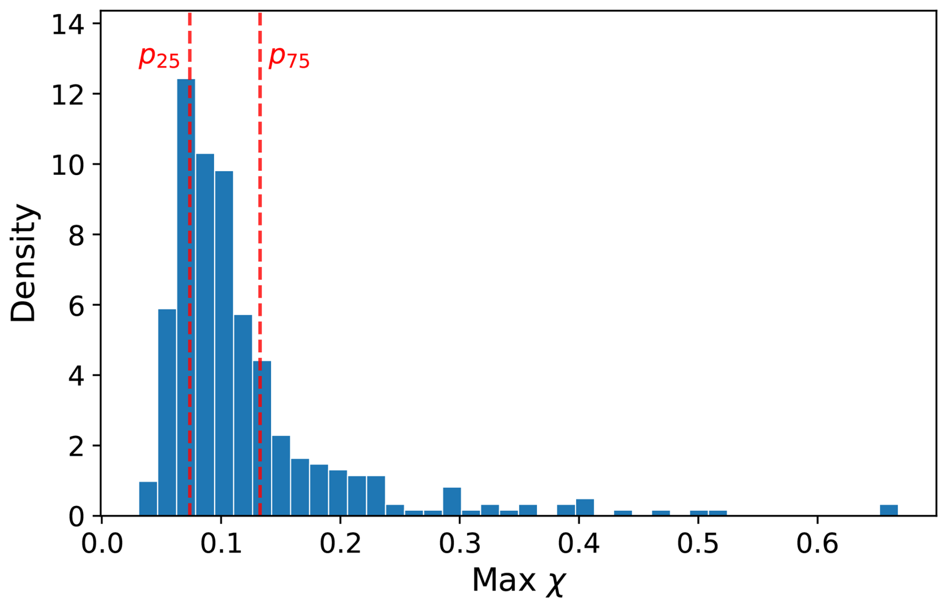
Figure 8 Density distribution of maximum χ for individual tracked particles over their lifetime in the stratocumulus-topped boundary layer. The 25th (p₂₅) and 75th (p₇₅) percentiles of the maximum χ are indicated with red dashed lines.

The diversity of pathways in the evaporation regime contrasts with the adiabatic growth regime, where droplets follow nearly uniform growth paths. In the entrainment and descent regime, trajectories diverge: some parcels are strongly diluted by entrainment (near the p90 line in Fig. 7e), while others experience minimal dilution, following the strong downdraft circulation (near the p50 line in Fig. 7e). To better understand the evolution of these diverse pathways and how microphysical properties diverge, we show changes in mixing-related properties for individual particle trajectories in the χ–z phase space (Figs. 9 and 10). We categorized droplets based on the 25th (χ=0.08) and 75th (χ=0.14) percentiles of their maximum lifetime χ values (Fig. 8). Droplets within parcels subject to strong entrainment-driven dilution experience high maximum χ>0.14 (first row), while the second and third rows show droplets with intermediate ($\mathrm{0.08}\le \mathit{\chi }\le \mathrm{0.14}$) and low (χ<0.08) maximum values, respectively. In all cases, d_r remains below 0.1 during ascent and increases when W<0, particularly for parcels with higher χ (Fig. 9c, f, and i).

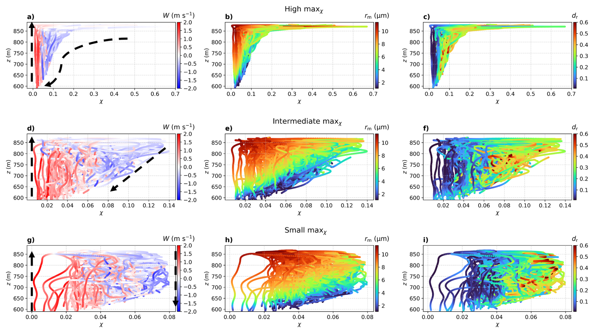
Figure 9 Particle trajectories in the χ–z phase space, where different colors of dots indicate: the W (first column), r_m (second column), d_r (third column). The first row shows trajectories with the maximum χ>0.14, the third row shows trajectories where the maximum χ≤0.08, and the second row shows trajectories with intermediate values, where the maximum χ lies between these two conditions. In panels (a), (d), and (g), the dashed black arrows indicate inferred droplet motion directions based on the vertical velocity W.

While most droplets descend without experiencing a substantial decrease in S, only a fraction are strongly diluted by entrainment, where S decreases as χ increases (Fig. 10e). For these droplets, S increases and χ decreases again after reaching its peak, indicating the restoration of S following turbulent mixing and evaporation, as well as further homogenization within the cloud. Notably, supersaturation fluctuation (σ_S) reaches a maximum at the cloud top while χ increases, further indicating entrainment and mixing. As r_m decreases and d_r increases rapidly during mixing and evaporation (Fig. 9b and c), these droplets descend and evaporate in a new state characterized by modified r_m and d_r. Conversely, droplets that do not experience high χ descend with a continuous state obtained at the end of the adiabatic growth regime, characterized by maximum r_m and minimum d_r (Fig. 9h and i).

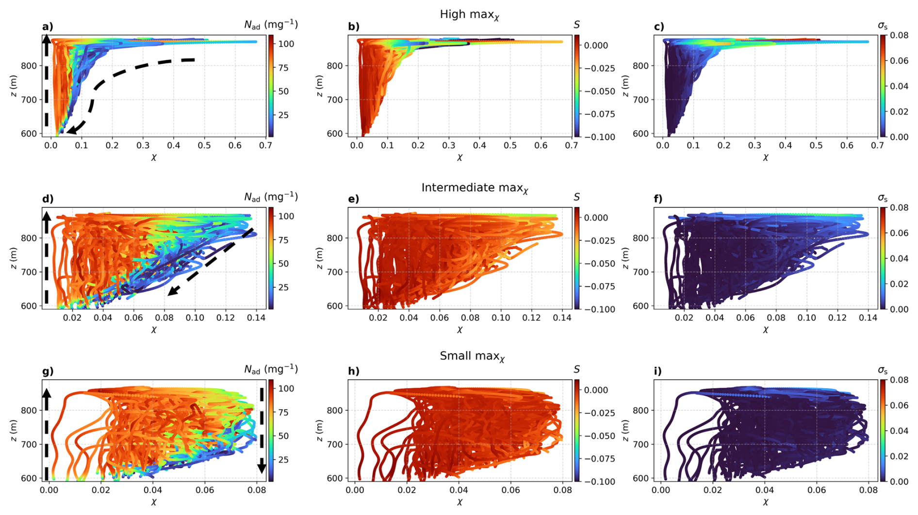
Figure 10 Particle trajectories in the χ–z phase space, where different colors of dots indicate: the N_ad (first column), S (second column), and σ_S (third column). The first row shows trajectories with the maximum χ>0.14, the third row shows trajectories where the maximum χ≤0.08, and the second row shows trajectories with intermediate values, where the maximum χ lies between these two conditions. In panels (a), (d), and (g), the dashed black arrows indicate inferred droplet motion directions based on the vertical velocity W.

Thus, for droplets within parcels subject to minimal dilution, r_m is primarily a function of altitude (Fig. 9h). At the same altitude, r_m is only slightly smaller at higher χ, regardless of whether the droplets are ascending or descending (Fig. 9g). Meanwhile, d_r is larger during descent (Fig. 9i), reflecting the broadening of the droplet size distribution due to evaporation in the absence of the collision-coalescence process. Along these trajectories, S remains high, while χ and σ_S remain low, suggesting that these droplets likely ascend and descend with negligible influence from entrainment. Furthermore, while both droplet groups undergo evaporation during descent, their initial r_m and d_r differ based on whether they reached a new state after mixing. This divergence leads to distinct evolution paths in the r_m–d_r phase space.

Another difference between the ascending and descending pathways is the evolution of droplet number concentration. To separate the decrease in N_c caused by simple entrainment dilution from that caused by mixing-induced evaporation, we examine the dilution-corrected number concentration, defined as $N_{\text{ad}}=N_{\mathrm{c}}/(\mathrm{1}-\mathit{\chi })$. Here, the subscript “ad” denotes the adiabatic value, representing the concentration expected in an undiluted parcel. Specifically, N_ad is substantially lower at higher altitudes when parcels are strongly diluted by entrainment (Fig. 10a) compared to those experiencing minimal dilution (Fig. 10g). This distinct reduction is also evident in the r_m–d_r phase space, where parcels subject to strong entrainment-driven dilution exhibit a rapid decrease in N_ad (Fig. 10a). This decrease, representing droplet loss beyond simple dilution, is consistent with inhomogeneous mixing, wherein some droplets completely evaporate in locally subsaturated environments while others remain relatively unaltered. The localized increase in σ_S further supports the conclusion that SGS supersaturation variability, as resolved by the LEM, drives this selective evaporation. These findings align with recent observational studies suggesting that inhomogeneous mixing signals are prevalent near the top of Sc clouds (Yeom et al., 2021).

However, we cannot ensure that $N_{\mathrm{c}}/(\mathrm{1}-\mathit{\chi })$ has fully isolated the effects of evaporation from entrainment-driven dilution. While the spatial distribution of the mixing signal indicates stronger inhomogeneous characteristics near the cloud top and homogeneous-like features below, it is questionable whether changes observed in the lower cloud should be interpreted as a result of active entrainment, especially since the majority of parcels descending with the STBL vertical circulation experience minimal dilution through entrainment. These uncertainties highlight a fundamental ambiguity in interpreting in situ observations of r_m and N_c as indicators of mixing type, particularly when a precise estimation of χ is unavailable.

To resolve this ambiguity, the maps of Da_phase, Da_evap, and the ratio ${\mathit{\tau }}_{\text{phase}}/{\mathit{\tau }}_{\text{evap}}$ in the χ–z phase space (Fig. 11) quantify the varying inhomogeneous and homogeneous mixing signals at the same height. Here, the Damköhler number is defined generally as

$$\begin{array}{}\text{(7)}& {\displaystyle }{\displaystyle }\mathit{Da}={\displaystyle \frac{{\mathit{\tau }}_{\text{mix}}}{{\mathit{\tau }}_{\text{micro}}}},\end{array}$$

where the mixing timescale (Baker and Latham, 1979; Baker et al., 1980) is

$$\begin{array}{}\text{(8)}& {\displaystyle }{\displaystyle }{\mathit{\tau }}_{\text{mix}}={\left({\displaystyle \frac{l^{\mathrm{2}}}{\mathit{\epsilon }}}\right)}^{\frac{\mathrm{1}}{\mathrm{3}}}.\end{array}$$

Here, l represents the length scale of scalar inhomogeneity caused by entrainment, which breaks down to the Kolmogorov length scale through turbulent motion. Since the entrainment length scale l varies with the size of the entrained blobs, we estimate the mixing length using χ as $l=(\mathit{\chi }\cdot \mathrm{\Delta }x\cdot \mathrm{\Delta }y\cdot \mathrm{\Delta }z{)}^{\mathrm{1}/\mathrm{3}}$. Notably, using the equivalent geometric LES grid lengthscale (≈7.9 m) as a proxy for l results in a larger τ_mix but does not alter the conclusions. The relevant microphysical timescales are the phase relaxation time

$$\begin{array}{}\text{(9)}& {\displaystyle }{\displaystyle }{\mathit{\tau }}_{\text{phase}}={\displaystyle \frac{\mathrm{1}}{\mathrm{4}\mathit{\pi }{D}_{\mathrm{v}}{r}_{\mathrm{m}}{N}_{\mathrm{c}}}}\end{array}$$

and the evaporation timescale

$$\begin{array}{}\text{(10)}& {\displaystyle }{\displaystyle }{\mathit{\tau }}_{\text{evap}}=-{\displaystyle \frac{r_{\mathrm{m}}^{\mathrm{2}}}{\mathrm{2}GS}},\end{array}$$

defined only in subsaturated regions with S<0 (Squires, 1952; Lehmann et al., 2009; Tölle and Krueger, 2014). Here, D_v is the molecular diffusion coefficient for water vapor, and $G={\left(F_{\mathrm{d}}+F_{\mathrm{k}}\right)}^{-\mathrm{1}}$ is the condensational growth parameter that summarizes the effects of vapor diffusion and heat conduction on condensation, with F_d, a coefficient associated with vapor diffusion, and F_k, associated with heat conduction (Yau and Rogers, 1996). Theoretically, when Da≫1, turbulent mixing is slower than the microphysical response, favoring inhomogeneous mixing. Conversely, when Da≪1, turbulent mixing is fast enough to homogenize the subsaturated entrained air with the saturated cloud air before droplets respond, leading to homogeneous mixing.

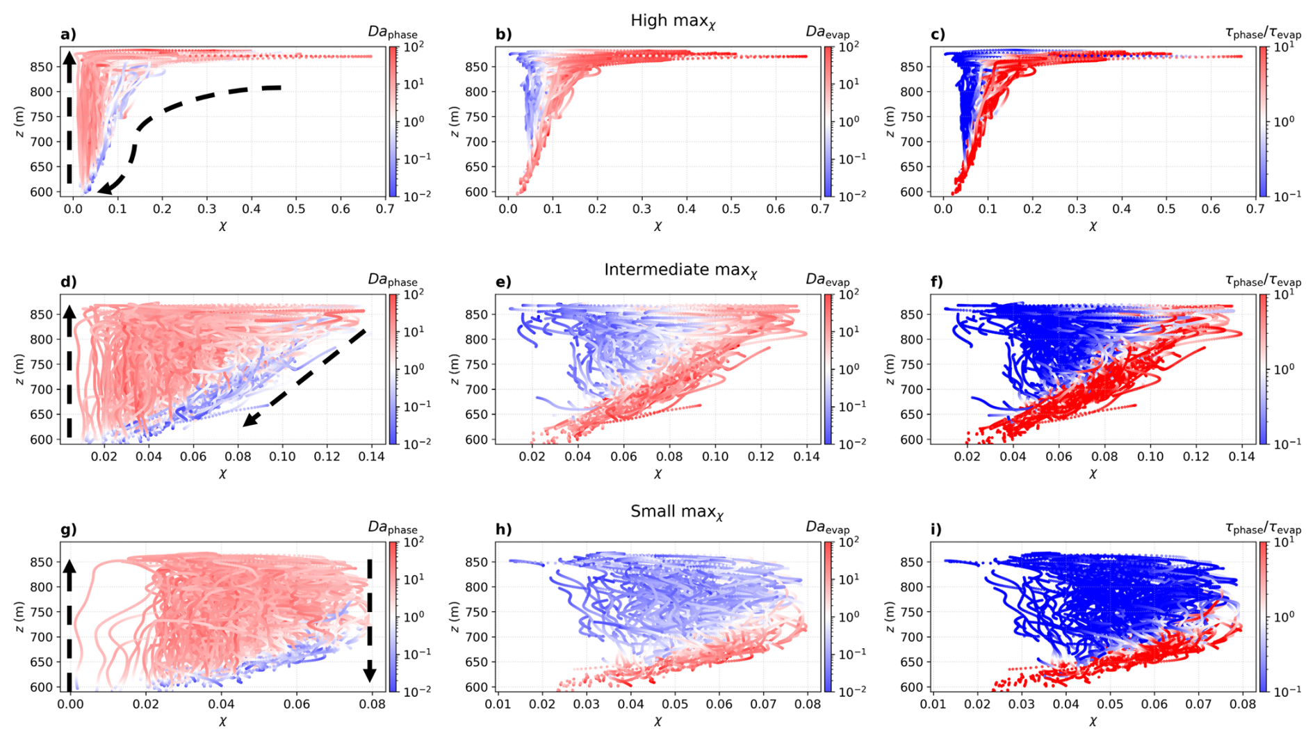
Figure 11 Particle trajectories in the χ–z phase space, where different colors of dots indicate: the Da_phase (first column), Da_evap (second column), ${\mathit{\tau }}_{\text{phase}}/{\mathit{\tau }}_{\text{evap}}$ (third column). The first row shows trajectories with the maximum χ>0.14, the third row shows trajectories where the maximum χ≤0.08, and the second row shows trajectories with intermediate values, where the maximum χ lies between these two conditions. In panels (a), (d), and (g), the dashed black arrows indicate inferred droplet motion directions based on the vertical velocity W.

While mixing scenarios have often been characterized using a single Damköhler number constructed from one microphysical response time (e.g. Baker et al., 1980; Burnet and Brenguier, 2007), recent work has highlighted the limitations of such single-parameter descriptions and the need to consider multiple thermodynamic timescales (Lehmann et al., 2009; Jeffery, 2007; Lu et al., 2018a; Fries et al., 2021). Therefore, we define two Damköhler numbers:

$$\begin{array}{}\text{(11)}& {\displaystyle }{\mathit{Da}}_{\text{phase}}={\displaystyle \frac{{\mathit{\tau }}_{\text{mix}}}{{\mathit{\tau }}_{\text{phase}}}}\text{ and }{\mathit{Da}}_{\text{evap}}={\displaystyle \frac{{\mathit{\tau }}_{\text{mix}}}{{\mathit{\tau }}_{\text{evap}}}},\end{array}$$

which represent the supersaturation relaxation-based and evaporation-based Damköhler numbers, respectively. Here, Da_phase measures how efficiently phase relaxation can restore supersaturation relative to turbulent mixing, whereas Da_evap measures how efficiently droplets can evaporate before the mixed air is re-saturated. In addition, we use the ratio between the two Damköhler numbers, ${\mathit{\tau }}_{\text{phase}}/{\mathit{\tau }}_{\text{evap}}$, which is closely related to the parameter suggested by Fries et al. (2021) and corresponds to the potential evaporation parameter of Pinsky et al. (2016).

In the high-χ regime (first row of Fig. 11), parcels subject to strong entrainment-driven dilution frequently exhibit Da_phase>1 (Fig. 11a) and Da_evap>1 (Fig. 11b), alongside a ratio of ${\mathit{\tau }}_{\text{phase}}/{\mathit{\tau }}_{\text{evap}}\gtrsim \mathrm{1}$ (Fig. 11c). This combination is consistent with an inhomogeneous mixing scenario, in which a subset of droplets evaporates completely while the remaining droplets maintain a relatively large r_m. As these parcels descend, Da_phase tends to decrease (Fig. 11a), whereas Da_evap remains greater than unity (Fig. 11b). Consequently, reliance on Da_phase alone might falsely indicate a transition toward homogeneous mixing during descent. The persistently high Da_evap, however, contradicts this interpretation. These parcels retain the signature of inhomogeneous mixing (depleted N_c, high Da_evap) well below the cloud top, even as a consistent decrease in χ indicates no further active entrainment dilution but mixing with boundary layer air. This occurs because they descend through air that remains incompletely homogenized, creating an environment more subsaturated than would be expected from adiabatic descent alone.

In contrast, trajectories that remain in the low-χ regime throughout their lifetime (third row of Fig. 11) tend to occupy regions with smaller Da_evap (Fig. 11h) but relatively large Da_phase (Fig. 11g), and with ${\mathit{\tau }}_{\text{phase}}/{\mathit{\tau }}_{\text{evap}}<\mathrm{1}$ (Fig. 11i). In this regime, phase relaxation is fast compared to both turbulent mixing and evaporation. This implies that adiabatic warming during descent is the primary source of droplet evaporation, without additional subsaturation caused by entrainment and dilution. These signatures are consistent with a homogeneous mixing-like response during descent, in which droplets gradually adjust r_m under a comparatively uniform supersaturation field without a substantial decrease in N_c, aside from weak entrainment-driven dilution at the cloud top. Moreover, as χ generally decreases during the descent, this implies no further strong effect of entrainment dilution during the descent. Crucially, this implies that the homogeneous-mixing-like signature often observed deeper in the cloud is not necessarily due to active entrainment and mixing at that level. Instead, it reflects droplet evaporation in weakly diluted, near-adiabatic parcels descending via the STBL vertical circulation (Telford and Chai, 1980; Wang et al., 2009).

The corresponding maps of the absolute timescales τ_mix, τ_phase, and τ_evap (Fig. 12) clarify why these diagnostics separate the regimes. The mixing timescale τ_mix varies relatively modestly across the χ–z phase space (Fig. 12a and g), whereas τ_phase and τ_evap exhibit much stronger spatial contrasts. Therefore, changes in Da_phase and Da_evap are driven mainly by the two microphysical timescales. The phase relaxation time τ_phase is strongly related to N_c: regions with strongly reduced N_c after complete evaporation events exhibit larger τ_phase (Fig. 12b), while most other regions show much shorter τ_phase (Fig. 12h). The evaporation timescale τ_evap behaves inversely, being large in nearly saturated regions and decreasing rapidly with increasing subsaturation (Fig. 12c and i). Consequently, the ratio ${\mathit{\tau }}_{\text{phase}}/{\mathit{\tau }}_{\text{evap}}$ serves as a direct indicator of where complete droplet evaporation is likely. This ratio is significantly higher for high maximum-χ parcels, reflecting their tendency toward complete evaporation, and remains much lower for low maximum-χ parcels until they reach the cloud base. Taken together, using ${\mathit{\tau }}_{\text{phase}}/{\mathit{\tau }}_{\text{evap}}$ provides a natural separation between regimes where droplets are prone to complete evaporation due to entrainment-induced dilution and regimes where supersaturation is restored quickly enough to prevent substantial droplet loss.

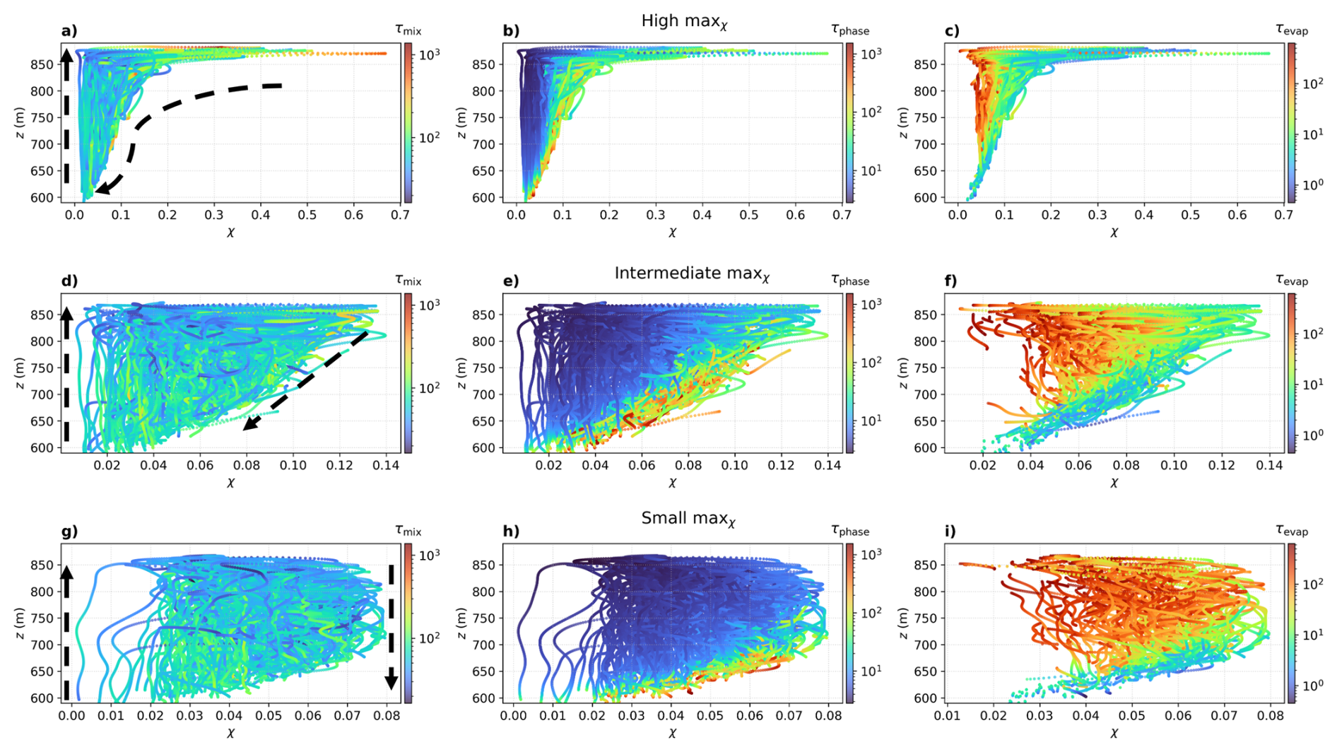
Figure 12 Particle trajectories in the χ–z phase space, where different colors of dots indicate: the mixing timescale τ_mix (first column), the phase-change timescale τ_phase (second column), and the evaporation timescale τ_evap (third column). The first row shows trajectories with the maximum χ>0.14, the third row shows trajectories where the maximum χ≤0.08, and the second row shows trajectories with intermediate values, where the maximum χ lies between these two conditions. In panels (a), (d), and (g), the dashed black arrows indicate inferred droplet motion directions based on the vertical velocity W.

These results highlight a contrast based on Lagrangian history. Parcels strongly diluted by entrainment near the cloud top are dominated by the inhomogeneous mixing signature. During descent, these parcels undergo gradual evaporation by adiabatic warming. Because of their greater subsaturation and decreased N_c, the droplets evaporate completely at a higher location in the cloud (Figs. 6l and 7f). Conversely, weakly diluted parcels descending near-adiabatically via the STBL circulation show a homogeneous-mixing-like signature driven solely by evaporation in the adiabatically descending parcel, rather than by active mixing events. These distinct Lagrangian histories explain why snapshots of r_m and N_c at a given altitude can simultaneously contain the imprints of both inhomogeneous and homogeneous mixing signatures, even without active entrainment events.

3.3.4 Deactivation Regime (S<0)

Droplets transition into the deactivation regime at the end of their life cycle near the cloud base (Fig. 7f). In this regime, the relationship between $\mathrm{d}{r}_{\mathrm{m}}/\mathrm{d}t$ and $\mathrm{d}{d}_{\mathrm{r}}/\mathrm{d}t$ is complex, as r_m decreases while d_r increases for larger r_m, but decreases for smaller r_m. The decrease in r_m is due to the evaporation of droplets. For larger r_m, d_r initially increases, as observed in the entrainment and descent regime. However, as the droplets approach complete evaporation, d_r decreases since only a small number of droplets remain. Therefore, this regime is opposite to the activation regime with substantial deactivation (Fig. 6l). Note that this regime does not overlap with the activation regime, because r_m and d_r are generally larger in the deactivation regime compared to the activation regime, indicating a stronger spatial variability in deactivation. Moreover, since particle trajectories are only tracked for q_c>0, an abrupt loss of liquid water near the point of complete evaporation may result in a bias toward retaining large r_m values as the final recorded state.

4 Complete Expression of Droplet Evolution Pathway

As demonstrated in Sect. 3.2, the growth phase of droplet evolution follows the analytical solution (Eq. 5) derived by Liu et al. (2006), which is grounded in classical diffusional growth theory. Starting from the condensational growth equation

$$\begin{array}{}\text{(12)}& {\displaystyle }{\displaystyle \frac{\mathrm{d}r}{\mathrm{d}t}}={\displaystyle \frac{SG}{r}},\end{array}$$

one may equivalently write $\frac{\mathrm{1}}{\mathrm{2}}\mathrm{d}\left(r^{\mathrm{2}}\right)/\mathrm{d}t=SG$, showing that condensational growth increases r² at a rate set by S and G.

To relate distribution width to the mean growth, Liu et al. (2006) define a relative deviation $x=(r-r_{\mathrm{m}})/r_{\mathrm{m}}$ so that $r=r_{\mathrm{m}}(\mathrm{1}+x)$ with $\stackrel{\mathrm{‾}}{x}=\mathrm{0}$. Substituting this into Eq. (12) and linearizing $\mathrm{1}/(\mathrm{1}+x)\approx \mathrm{1}-x$ yields an evolution equation of the form (their Eq. (4))

$$\begin{array}{}\text{(13)}& {\displaystyle }{\displaystyle }(\mathrm{1}+x){\displaystyle \frac{\mathrm{1}}{\mathrm{2}}}{\displaystyle \frac{\mathrm{d}\left(r_{\mathrm{m}}^{\mathrm{2}}\right)}{\mathrm{d}t}}+r_{\mathrm{m}}^{\mathrm{2}}{\displaystyle \frac{\mathrm{d}x}{\mathrm{d}t}}=SG(\mathrm{1}-x).\end{array}$$

Averaging this over the droplet population yields their Eq. (5):

$$\begin{array}{}\text{(14)}& {\displaystyle }{\displaystyle \frac{\mathrm{1}}{\mathrm{2}}}{\displaystyle \frac{\mathrm{d}\left(r_{\mathrm{m}}^{\mathrm{2}}\right)}{\mathrm{d}t}}=SG.\end{array}$$

By combining these two equations and using $d_{\mathrm{r}}^{\mathrm{2}}=\stackrel{\mathrm{‾}}{x^{\mathrm{2}}}$, this leads to

$$\begin{array}{}\text{(15)}& {\displaystyle }{\displaystyle \frac{\mathrm{1}}{d_{\mathrm{r}}^{\mathrm{2}}}}{\displaystyle \frac{\mathrm{d}\left(d_{\mathrm{r}}^{\mathrm{2}}\right)}{\mathrm{d}t}}=-\mathrm{2}{\displaystyle \frac{\mathrm{1}}{r_{\mathrm{m}}^{\mathrm{2}}}}{\displaystyle \frac{\mathrm{d}\left(r_{\mathrm{m}}^{\mathrm{2}}\right)}{\mathrm{d}t}}.\end{array}$$

Integrating this relationship yields the characteristic inverse-square scaling $d_{\mathrm{r}}\propto r_{\mathrm{m}}^{-\mathrm{2}}$ (Eq. 5), providing a quantitative expression of condensational narrowing during adiabatic ascent. For the full derivation, see Liu et al. (2006) (their Eqs. 2–9).

However, this analytical formulation is insufficient for the decay phase (S<0), where evaporation and mixing induce nonlinear and path-dependent spectral broadening. While applying Eq. (5) to this regime captures the overall decreasing trend, it fails to reproduce the observed concave curvature, resulting in lower correlation coefficients (r²=0.5–0.8; see light-gray dashed line in Fig. 13). Given that an analytical derivation is complicated by the stochastic nature of entrainment, we instead formulate an empirical model based on geometric constraints. This model is constructed to satisfy two physical boundary conditions observed in our simulations: (1) a maximum dispersion (d_{r, max}) at the limit of small radii, and (2) a vanishing dispersion as the mean radius approaches a system maximum (r_{m, max}), representing the spectral narrowing limit governed by condensational growth.

Figure 13 Frequency distribution in the r_m–d_r phase space for S<0 for the (a) N50, (b) N100, and (c) N200 cases. Black dots represent the most frequent value (mode) in each r_m bin. The light-gray dashed line shows the fit of the analytical growth-phase equation (Eq. 5) to the S<0 data. The red lines represent the empirical fits for this evaporation pathway using the final quadratic formulation (the S<0 part of Eq. 16 as solid and the S≥0 part of Eq. 16 as dashed). All fits are based on the median d_r value in each r_m bin.

To satisfy these conditions while capturing the observed curvature, we adopt a quadratic formulation. Combining the analytical growth term with this empirical decay formulation, we propose the following piecewise function for the complete evolution pathway:

$$\begin{array}{}\text{(16)}& {\displaystyle }{\displaystyle }{d}_{\mathrm{r}}=\left\{\begin{array}{ll}{d}_{\text{r, 0}}\frac{r_{\text{m, 0}}^{\mathrm{2}}}{r_{\mathrm{m}}^{\mathrm{2}}}& \text{if }S\ge \mathrm{0},\\ d_{\text{r, max}}\left(\mathrm{1}-\frac{r_{\mathrm{m}}^{\mathrm{2}}}{r_{\text{m, max}}^{\mathrm{2}}}\right)& \text{if }S<\mathrm{0}.\end{array}\right.\end{array}$$

The results of Eq. (16), fitted to the 50th percentile of the frequency distributions over the final 2 h of simulation, are shown as solid lines in Fig. 13 for the N50, N100, and N200 cases. The fitted values of d_{r, max} are 0.39, 0.40, and 0.41, respectively, while r_{m, max} values are 14.9, 11.8, and 9.4 µm, with all fits yielding r²>0.98. While d_{r, max} exhibits only modest variation across aerosol scenarios, r_{m, max} decreases noticeably with increasing N_a, consistent with liquid water being partitioned among a larger number of droplets. The relative insensitivity of d_{r, max} to N_a suggests that a fixed value in the range of 0.3–0.4, commonly observed in stratocumulus clouds (Pawlowska et al., 2006), may serve as a useful approximation.

5 Summary and Conclusion

Maritime stratocumulus (Sc) clouds play an important role in Earth's radiative budget by reflecting incoming solar radiation (Wood, 2012). However, our lack of understanding of the variation of key parameters determining the cloud's optical properties, such as the droplet size distribution (DSD), makes clouds a key source of model uncertainty (Boucher et al., 2013). In this study, we investigate the evolution of droplets, focusing on how DSD shape parameters, the mean droplet radius (r_m) and droplet radius relative dispersion (d_r), evolve by tracking individual cloud droplets. For this purpose, we employ the L³ model that couples a large-eddy simulation (LES) model with a Lagrangian cloud model (LCM), and the linear eddy model (LEM) to accurately represent entrainment and mixing, a key process in determining DSD shape (Lim and Hoffmann, 2023).

We find that the evolution of droplet size distribution (DSD) shape parameters follows characteristic trajectories in the r_m–d_r phase space, governed by the large-scale circulation of the stratocumulus-topped boundary layer (STBL). Droplets undergo distinct transitions, including activation, condensational growth, entrainment-driven evaporation, and descent within downdrafts, each constituting a stage of an “aging” pathway. Based on supersaturation conditions, we classify the droplet population into four microphysical regimes as follows:

1. Activation (S≥0, small r_m): droplets activate, increasing r_m and broadening d_r.

2. Adiabatic growth (S≥0, small d_r): condensational growth narrows the DSD while increasing r_m, following the analytical parcel theory ($d_{\mathrm{r}}\propto r_{\mathrm{m}}^{-\mathrm{2}}$).

3. Entrainment and descent (S<0): evaporation drives a decrease in r_m and an increase in d_r. Critically, droplets in this regime do not follow a single pathway; their trajectories diverge in the r_m–d_r phase space depending on parcel-specific entrainment history (mixing fraction χ).

4. Deactivation (S<0, near cloud base): the final evaporation stage, where large droplets persist longer than small ones, briefly widening d_r before full deactivation.

Importantly, this study helps resolve a fundamental ambiguity in interpreting mixing mechanisms in stratocumulus clouds. While vertical profiles of droplet number concentration (N_c) and mean radius (r_m) often suggest a transition from inhomogeneous mixing at cloud top to homogeneous mixing below (Wang et al., 2009; Yum et al., 2015; Yeom et al., 2021), our trajectory-resolved analysis shows that much of this vertical structure arises from sorting of parcels with different entrainment histories within the STBL circulation (Telford and Chai, 1980; Wang et al., 2009). Specifically, the apparent mixing regime is controlled primarily by the Lagrangian entrainment history (summarized by the mixing fraction χ) rather than instantaneous altitude. Parcels subject to strong entrainment-driven dilution (high χ) exhibit robust inhomogeneous-mixing signatures at cloud top, characterized by a rapid reduction in N_c with only weak changes in r_m under strong subsaturation.

In contrast, the pervasive homogeneous-mixing-like signature at lower altitudes arises largely from parcels that descend adiabatically within the STBL downdrafts with minimal dilution (low χ). In these parcels, r_m decreases mainly due to adiabatic warming during descent, while N_c remains approximately conserved, producing vertical profiles that mimic homogeneous mixing without requiring active entrainment and mixing at that level. These results demonstrate that interpretations based solely on Eulerian snapshots of N_c and r_m can conflate local mixing with the imprint of pathway-dependent Lagrangian histories.

Consequently, to provide a more accurate assessment, we suggest using the evaporation-based Damköhler number Da_evap or the timescale ratio ${\mathit{\tau }}_{\text{phase}}/{\mathit{\tau }}_{\text{evap}}$ as a better parameter for diagnosing mixing scenarios (Pinsky et al., 2016; Fries et al., 2021) than using a Da based on the single microphysical timescale. This approach is supported by the fact that inhomogeneous mixing is fundamentally controlled by whether a subset of droplets can completely evaporate. In particular, ${\mathit{\tau }}_{\text{phase}}/{\mathit{\tau }}_{\text{evap}}$ depends only on the microphysical state variables r_m, N_c, and S and does not require explicit knowledge of τ_mix, making it particularly attractive. While both Da values indicate inhomogeneous mixing near the cloud top, each Da indicates different mixing scenarios during descent without active entrainment events. Therefore, a single Da may give a false classification of an inhomogeneous to homogeneous mixing scenario, but the combination of both can successfully indicate if the parcel is strongly diluted or not, which is useful to diagnose different entrainment-driven dilution histories.

While our regime classification spans the full vertical structure of the STBL, observational access to this regime space is inherently limited. As a result, the complete trajectory of DSD evolution remains poorly constrained in most field observations. Although some observational studies have reported phase-space patterns consistent with portions of our defined regimes (e.g. Lu et al., 2020), comprehensive vertical coverage is needed to resolve the full aging pathway. Our Lagrangian framework overcomes this methodological limitation by providing a trajectory-resolved depiction of regime transitions across the full STBL depth, offering a coherent framework for interpreting in situ observations within the broader context of cloud evolution.

Building on these regime definitions, we propose an empirical formulation, combined with the analytical expression of Liu et al. (2006), that expresses d_r as a function of r_m. This formulation explicitly captures the inverse-square DSD narrowing governed by condensational growth and the nonlinear broadening driven by entrainment and dilution. This unified expression provides a practical framework for incorporating DSD aging variability into microphysical parameterizations in cloud models.

Our findings underscore the significance of DSD aging in preconditioning the onset of precipitation (e.g. Seifert and Beheng, 2006). Broader DSDs, shaped by diverse droplet growth pathways and entrainment-induced dilution and mixing histories, can enhance the potential for rain formation or reduce a cloud's ability to reflect incoming solar radiation. These results emphasize that droplet-scale evolution under varying thermodynamic and dynamic conditions governs not only the DSD shape but also key radiative and precipitation-relevant properties, highlighting the need for improved representation of DSD variability in large-scale models.