A spectral perspective of the clear-sky OLR variability driven by ENSO

The study of short-term unforced variability of the Earth radiative budget can provide much information for the understanding of the long-term effect of external radiative forcing, related to the present climate change. In this regard, inter-annual variability of the Outgoing Longwave Radiation (OLR) is strongly shaped by El-Niño Southern Oscillation (ENSO). So far, the relationship between the OLR and ENSO has been investigated using broadband satellite-based observations, such as those of the Clouds and Earth Radiant Energy System, finding that the peak of the OLR response lags the peak of ENSO activity. However, such observations cannot directly inform on the individual processes that drive the radiative response to ENSO. Here, we exploit the spectrally-resolved clear-sky OLR fluxes – measured by the Infrared Atmospheric Sounding Interferometer and the Atmospheric Infrared Sounder instruments – to expand the observational analysis of ENSO's radiative response, showing that its intensity and lag vary along the spectral dimension. The spectral fingerprint of water vapor, surface and air temperature, and ozone feedback is then calculated using a set of spectral kernels to evaluate the role of individual processes in building the overall response. Results show a strong contribution coming from the ozone absorption band, along with a contribution of opposite sign coming from the core of the carbon dioxide band, which is mainly affected by stratospheric temperature. This analysis confirms the important role of the spectral dimension to study climate processes. In this regard, it sets the basis for a spectral diagnostic to evaluate how ENSO driven variability is reproduced by climate models.

1 Introduction

The Outgoing Longwave Radiation (OLR) encompasses the energy flux (W m⁻²) emitted by the Earth towards space across the far and thermal infrared spectral regions (from 100 to about 3330 cm⁻¹) and represents the main mechanism by which the climate system loses energy to maintain its thermal equilibrium. The long-term trend of the OLR bears the signal related to the increase of carbon dioxide concentration and other Greenhouse Gases (GHGs), driving the present-day climate change, as well as that of the system's radiative response, produced by the warming of the planet's surface and resulting climate feedbacks.

To monitor the changes in OLR emission through time we can rely on satellite measurements of the top-of-atmosphere (TOA) OLR. One of the most important instruments is the Clouds and Earth Radiant Energy System (CERES). It has flown since 2000 on board the Terra and Aqua platforms and it has now achieved more than 20 years of stable records of the Earth energy budget and its components. Despite that, the available observational records are not yet long enough to accurately quantify the long-term trend of the OLR and use it to constrain climate models feedbacks (Uribe et al., 2024). Indeed, the exact magnitude of climate feedbacks, which determine the ultimate warming of the planet in response to forcing, is still uncertain and Global Climate Models (GCMs) struggle to agree on a precise value. For example, a stronger positive cloud feedback in the Coupled Model Intercomparison Project phase 6 (CMIP6) is the cause of a higher Effective Climate Sensitivity (ECS) estimate, with values between 1.8–5.6 K, exceeding the range 2.1–4.7 K, obtained with the previous generation of models (CMIP5) (Zelinka et al., 2020). A possible way ahead is represented by the study of the planet's internal variability from observations. The OLR is in fact also subjected to fluctuations on seasonal and interannual timescales. Several research efforts have been focused on the study of the short-term variability to improve the understanding of feedback processes on longer timescales (Dessler et al., 2008; Dessler, 2010, 2013; Uribe et al., 2022).

On the inter-annual time scale, El-Niño Southern Oscillation (ENSO) is the dominant variability mode of the climate system. It causes changes in the Tropical Pacific Sea Surface Temperature (SST) coupled with changes in the above atmospheric circulation, affecting the Earth's climate on a global scale (McPhaden et al., 2020). ENSO induced perturbations to atmospheric and surface variables strongly affect the TOA OLR. Loeb et al. (2012) and Susskind et al. (2012) studied the effect of ENSO on the OLR using the first decade of measurements acquired by the CERES instrument. They both show that the OLR co-varies significantly with ENSO activity, assuming positive (negative) anomalies in correspondence to El-Niño (La-Niña) phase. The main radiative feedback driven by ENSO induced SST perturbations involves water vapor, temperature and clouds properties changes (Huang et al., 2021). Their evolution during the ENSO life cycle provides information on the feedbacks important for ENSO developing and maintenance. Particularly, the atmosphere exerts an overall positive feedback that act to strengthen ENSO during its developing phase (Kolly and Huang, 2018; Huang et al., 2021). This result is also confirmed by Ceppi and Fueglistaler (2021), which used measurements of broadband energy fluxes to investigate the time relationship between the net TOA Earth Radiative Budget (ERB) and ENSO.

All the works presented above examined ENSO driven variability using broadband OLR observations, which provide the total radiative flux integrated over the Infrared (IR) spectral range (e.g. 50–2000 cm⁻¹ for CERES). However, we can also rely on spectral OLR measurements (the integrand of the broadband radiance), which has consolidated since the beginning of this century thanks to the availability of instruments such as the Atmospheric Infrared Sounder (AIRS), the Infrared Atmospheric Sounding Interferometer (IASI) or the Cross-track Infrared Sounder (CrIS) (Brindley and Bantges, 2016). For instance, Huang and Ramaswamy (2008) investigated the OLR variability in relation to SST using spectral measurements acquired by the AIRS instrument. More recently, Raghuraman et al. (2023) analyzed trends in AIRS spectral radiances (2003–2021) and, combining these observations with simulations from the Geophysical Fluid Dynamics Laboratory general circulation model, separated climate feedbacks from radiative forcing and stratospheric adjustment associated with increasing greenhouse gas concentrations. The analysis of the trend of the first ten years of observations of IASI (from 2008 to 2017) revealed the spectral signature related to both the increase in GHGs concentration and ENSO variability across channels sensitive to water vapor and temperature (Whitburn et al., 2021). Using IASI observations, Roemer et al. (2023) calculated the net longwave (LW) spectral feedback parameter and directly observed the spectral fingerprint due to changes in relative humidity for an increasing value of global mean surface temperature.

In addition, spectral OLR have been proven to be a powerful method to assess climate model performance, allowing to reveal biases otherwise hidden by compensating effects when broadband fluxes are considered (Della Fera et al., 2023; Huang et al., 2007; Leroy et al., 2008; Huang et al., 2014). The study of the spectral radiative response to ENSO potentially allows to better constrain climate feedbacks and evaluate the performance of climate models, inspecting their representation of the coupled atmosphere-ocean dynamics (Andrews et al., 2015; Armour et al., 2024; Andrews et al., 2022). Indeed, there is evidence that the radiative response to ENSO is still not completely reproduced in both its amplitude and timing by climate models (Kolly and Huang, 2018; Planton et al., 2021; Ceppi and Fueglistaler, 2021).

The present work aims to demonstrate the value of the spectral dimension in OLR measurements for the understanding of the mechanisms that drive the radiative response to ENSO. Building on the analysis by Ceppi and Fueglistaler (2021), we first assess the OLR response to ENSO using CERES broadband observations. We then explore the potential of the spectral dimension to identify the processes that drive the timing and the magnitude of the OLR anomalies, comparing measurements acquired by IASI and AIRS instruments. Finally, the role of water vapor, surface and air temperature spectral feedback is investigated, calculating their radiative changes by means of spectral radiative kernels. Our analysis highlights the role of different feedback processes in driving OLR variability and we propose to apply it for a stricter evaluation of climate model performance.

The article is organized as follows: a description of the datasets and of the methodology applied is provided in Sect. 2; the results of the analysis are presented in Sect. 3; the main findings are discussed in Sect. 4, and final conclusions are drown in Sect. 5.

2 Data and Methods

2.1 Observational datasets

The analysis is based on clear-sky OLR spectral fluxes which are derived from radiance measurements acquired by two different sounders: the AIRS and IASI instruments.

The first is a grating array spectrometer which measures spectrally resolved radiances across three different bands, 650–1136, 1216–1613, 2170–2674 cm⁻¹ (Aumann et al., 2003). The corresponding fluxes have been derived by Huang et al. (2008) for both clear and all-sky observations of the instrument flying on board the Aqua satellite from November 2002 to present days. Simulated radiances have been used to fill the spectral gaps and extend the original spectral range below 650 cm⁻¹, down to 15 cm⁻¹. The final product consists of monthly mean spectral fluxes computed at 10 cm⁻¹ from 15 to 1995 cm⁻¹, with a horizontal resolution of 2° latitude by 2° longitude. Two separate flux products are provided for the two AIRS overpass times at the equator, 01:30 and 13:30 LT. In this study, we use the average of these two overpasses.

IASI is a Fourier transform spectrometer which measures radiances across the range from 645 to 2760 cm⁻¹, with a spectral resolution of 0.25 cm⁻¹ (Simeoni et al., 2004). We use the dataset of clear-sky spectral fluxes derived from measurements acquired by IASI on board the MetOp-A (October 2007–December 2021), as described in Whitburn et al. (2020). The dataset consists of monthly mean spectral fluxes for the period from January 2008 to October 2021. Spectral fluxes are provided over a 2° longitude by 2° latitude grid and span the wavenumber range from 645 to 2300 cm⁻¹, with a spectral resolution of 0.25 cm⁻¹. Two products are provided for night-time (21:30 LT at the equator) and daytime (09:30 LT at the equator) observations, respectively. As was as done for AIRS, these overpasses have been averaged. The same product is also available for data collected on board the MetOp-B (2013–today) and C (2017–today), however, for this study, the MetOp-A ensures the greatest temporal overlap with the AIRS and CERES datasets. It should be noted that the MetOp-A platform began drifting from its nominal orbit in autumn 2017, resulting in an earlier local time of the ascending node.

In addition to AIRS and IASI spectral fluxes, we used broadband OLR values derived from CERES measurements. CERES is a broadband radiometer with three channels that measure radiances across the whole spectrum (50–3000 cm⁻¹), the shortwave (2000–3000 cm⁻¹) and the atmospheric window (830–1250 cm⁻¹) regions, respectively (Wielicki et al., 1996). We use the CERES Energy Balanced and Filled (EBAF) Edition 4.1 data product (Loeb et al., 2020), which gathers data collected by different CERES instruments on board Terra and Aqua platforms since 2000. Two clear-sky products are available, one that only considers cloud-free observations and another that additionally applies a correction factor for a better comparison with climate models output, for which clear-sky fluxes are artificially produced by removing clouds from the flux calculation. The first product has been selected for consistency with IASI and AIRS observations. CERES-EBAF 4.1 provides monthly mean TOA OLR fluxes with an horizontal resolution of 1° per 1° and a temporal coverage from January 2000 to March 2022.

The main features of the three datasets are resumed in Table 1.

Loeb et al. (2020)Huang et al. (2008)Whitburn et al. (2020)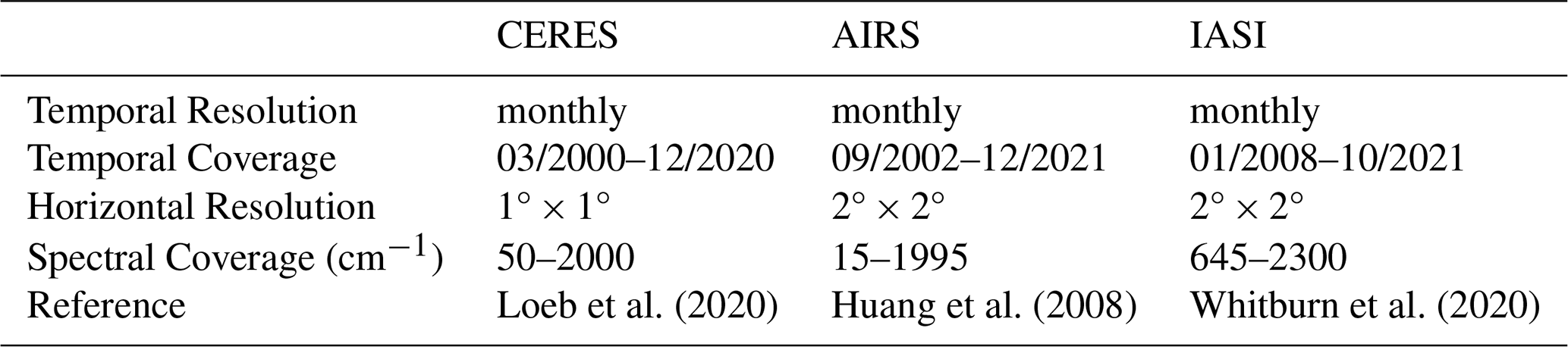

Table 1 Main features of the datasets used.

2.2 Spectral Radiative Kernels

Radiative kernels (or Jacobians) represent the partial derivative of the spectral flux or radiance with respect to specific climate variables, evaluated across the atmospheric levels. They can be used to estimate the OLR perturbation at the TOA resulting from changes in atmospheric and surface climate variables (Soden et al., 2008).

For this study we use a set of clear-sky spectral kernels developed by Della Fera et al. (2025). The kernels have been computed using the RTTOV model (Radiative Transfer model for the TIROS-N Operational Vertical Sounder) (Matricardi, 2009) and monthly mean profiles from the European Center for Medium-Range Weather Forecast (ECMWF) Reanalysis v5 (ERA5) dataset as the input for meteorological fields. The derivatives have been computed for three different years 2008, 2009, and 2010, and then averaged to obtain representative monthly kernels of surface and atmospheric temperature, water vapor and ozone. Furthermore, in order to obtain the derivatives of the spectral flux (W (m² cm⁻¹)⁻¹), radiance derivatives (W (m² cm¹ sr)⁻¹) were computed at three distinct viewing angles (24.29, 53.80, 77.74°). The resulting values were then integrated using Gaussian quadrature, which has been shown to yield accurate results for clear-sky radiative transfer calculations (Clough et al., 1992). More details regarding the construction of the spectral kernels can be found in Della Fera et al. (2025).

The resulting product consists of radiative kernels, averaged over 10 cm⁻¹ intervals, from 100 to 2300 cm⁻¹, spanning 17 pressure levels (hPa): 1000, 925, 850, 700, 600, 500, 400, 300, 250, 200, 150, 100, 70, 50, 30, 20, 10, on a horizontal grid of 2.5° longitude per 2.5° latitude. As an example, Figs. A1 and A2 show a comparison of the surface and air temperature kernels used in this study with the radiative kernels computed by Huang and Huang (2023) for the month of January. For the selected scenario, the differences between the two sets of radiative kernels are small, being within the 5 % for the tropical zone. Additional validation has been made to test the accuracy of using as input monthly mean versus instantaneous profiles for the meteorological fields, as done by Huang and Huang (2023) (not shown). It emerges that for the clear-sky case the differences between the two approaches are small (within the 1 %) and do not appear to be significant for the results of our analysis.

Finally, the change in the radiative flux associated to the change in each climate variable is obtained multiplying the respective radiative kernel by the anomaly of that variable and then, for 3D fields, summing over the pressure levels to obtain the total atmospheric response. Surface and atmospheric temperature, water vapor and ozone fields are taken from the monthly ECMWF ERA5 reanalysis (Hersbach et al., 2023). Atmospheric variables are selected on the same 17 pressure levels used for the radiative kernels computation. Anomalies of meteorological fields are computed relative to the monthly mean from January 2008 to December 2020, the period selected for the analysis.

2.3 The Niño 3.4 index

The Niño 3.4 index has been used as a measure of ENSO phase and magnitude. It is defined as the average SST anomaly over the Niño 3.4 region (5° S–5° N, 170–120° W), smoothed with a five-month running mean (Trenberth, 1997). Area-averaged SSTs provided by the NOAA database have been used for its calculation (https://www.cpc.ncep.noaa.gov/data/indices/ersst5.nino.mth.91-20.ascii, last access: 15 April 2024). The resulting Niño 3.4 index is plotted in Fig. 1 for the years from January 2008 to December 2020. The period examined is characterized by two strong El-Niño events. The first peaked during the 2009–2010 winter and the second during the winter of 2015–2016. Two strong La-Niña events also occurred in the winter of 2007–2008 and 2010–2011.

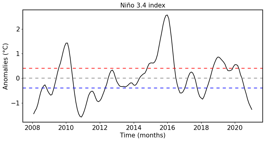
Figure 1 The Niño 3.4 from January 2008 to December 2020 calculated using the area-averaged SST provided by the NOAA-PSL database. The blue (red) horizontal line marks the −0.4 (0.4) °C temperature anomalies, above which ENSO episodes are classified as La-Niña (El-Niño).

2.4 Lagged regression analysis

The time relationship between OLR anomalies and ENSO activity has been investigated through a lagged regression analysis, performed over the period from January 2008 to December 2020, which is common to all the observational datasets.

All the datasets have been regridded to a common grid of 2.5° latitude per 2.5° longitude, through a bilinear interpolation. Then, the monthly OLR anomaly has been calculated by subtracting the monthly climatology, relative to the period considered, from the OLR time series. In order to better isolate the internal variability signal from the one related to the increase in GHGs concentration, we removed the linear trend of the OLR anomaly over the given period.

Lagged regressions have been calculated performing a linear regression between the radiative anomaly and the Niño 3.4 index as follow:

$$\begin{array}{}\text{(1)}& y=m\cdot x+q\end{array}$$

In Eq. (1), y and x are the OLR anomaly and Niño 3.4 index time series, respectively, from January 2008 to December 2020; the variable x has been shifted one month at a time from −12 to +12 months, resulting in 25 regression coefficients, m, being obtained at the end of the procedure. The regression coefficients (units of W m⁻² K⁻¹) are a measure of the radiative perturbations driven by ENSO induced SST anomalies. We will refer to these as “ENSO feedback” for the rest of the paper, as done also by Kolly and Huang (2018) and Huang et al. (2021). The 95 % statistical significance of the regression coefficients has been assessed with a two-tailed t-test.

The analysis focused on the tropical zone (30° S–30° N), where the radiative perturbations induced by ENSO are strongest, and on values above ocean, to avoid introducing biases in the comparison of non-simultaneous measurements, which can arise from the rapid temperature variability typical of land surfaces (Huang and Yung, 2005; Whitburn et al., 2021).

3 Results

Here, we present the main results of the analysis, starting from the broadband fluxes and then moving to the spectral dimension.

3.1 Broadband LW radiative response to ENSO

The OLR response to ENSO variability is presented first from a broadband perspective. Figure 2 shows the tropical mean broadband OLR response to ENSO as a function of the time lag obtained using fluxes from CERES, IASI and AIRS. In the case of AIRS, the spectral fluxes are integrated over two different spectral ranges: from 50–1995 cm⁻¹, to be as consistent as possible with CERES, which encompasses the range from 50 to 2000 cm⁻¹, and from 645–1995 cm⁻¹, to match the spectral range encompassed by IASI. Note that, in order to be consistent with the definition of climate feedbacks, the sign of the OLR response has been inverted. Thus, a negative ENSO feedback corresponds to an enhanced OLR emission at the TOA, conversely, a positive feedback is associated with a decrease in OLR.

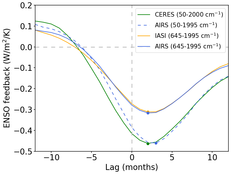
Figure 2 Lagged regressions of the tropical mean broadband OLR anomalies from CERES (green), AIRS (blue) and IASI (orange), respect to the Niño 3.4 index, from lag −12 to +12 months. The sign of the OLR has been inverted (negative feedback = positive OLR anomaly).

The radiative response depicted in Fig. 2 suggests an increase in OLR emission at the TOA associated to ENSO. In more detail, the total LW ENSO feedback becomes negative starting from about five months ahead of the ENSO peak. The negative peak is reached at a lag of 2 months, and the response gradually weakens thereafter. This result agrees with Ceppi and Fueglistaler (2021), who found a similar OLR response to ENSO in clear-sky conditions, suggesting that it is likely driven by the Planck effect.

When the entire spectral region from 50 to 2000 cm⁻¹ is accounted for, the OLR peak at the 2-months lag is of −0.46 ± 0.11 W m⁻² K⁻¹ for AIRS and −0.46 ± 0.12 W m⁻² K⁻¹ for CERES, whereas it decreases to −0.31 ± 0.05 W m⁻² K⁻¹ for AIRS and −0.31 ± 0.05 W m⁻² K⁻¹ for IASI, when the 645–1995 cm⁻¹ wavenumber range is considered. These values denote that approximately 30 % of the total OLR emission during ENSO is achieved between 50 and 645 cm⁻¹, confirming the importance of the Far-Infrared (FIR) spectral region (100–600 cm⁻¹) for the TOA ERB (Palchetti et al., 2020; Harries et al., 2008).

Although we find an excellent agreement in the magnitude of the OLR response peak between CERES and AIRS, the AIRS signal exhibits a delay of one month, peaking at 3-months lag, and a smaller value at negative lags, compared to CERES. Instead, the agreement between AIRS and IASI is excellent, with minor differences at negative lags.

3.2 ENSO spectral footprint from AIRS and IASI

In order to examine the factors that control the magnitude and timing of the LW ENSO feedback, we have extended the analysis to the spectral dimension. Lagged regressions between the tropical mean OLR anomalies and the Niño 3.4 index have been performed at each wavenumber encompassed by IASI and AIRS spectral fluxes. To enable a direct comparison, IASI spectra have been resampled to the same resolution as the AIRS dataset (10 cm⁻¹).

Results are showed in Fig. 3, which reports the spectral ENSO feedback as a function of wavenumbers and time lag (panels a and b), and for a time lag of two months (panel c), where the broadband response peaks. Different responses are obtained across the spectrum. Specifically, different spectral regions are associated with a characteristic lag, as well as a particular sign and magnitude of the ENSO feedback. The wings of the carbon dioxide absorption band (∼ 600–645 and ∼ 700–800 cm⁻¹), the atmospheric windows (∼ 800–1000 and ∼ 1100–1200 cm⁻¹) and the ozone absorption band (∼ 1000–1065 cm⁻¹) are all associated with a negative ENSO feedback. Below 600 cm⁻¹, where only AIRS simulated spectral fluxes are available, a widespread negative ENSO feedback emerges. The only positive feedback comes from the center of the carbon dioxide absorption band (∼ 645–700 cm⁻¹).

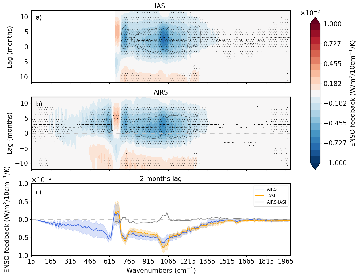
Figure 3 (a) Lagged regressions of the tropical mean spectral OLR anomalies from IASI respect to the Niño 3.4 index as a function of wavenumbers and lag. (b) Same as (a), but for AIRS. (c) Regression of the spectral OLR anomalies respect to the Niño 3.4 index at the 2-months lag for AIRS (blue) and IASI (orange), and their difference (gray). In panels (a) and (b), thinner black dots mark 95 % significance of the slopes, while thicker black dots mark the lag where the strongest radiative response occurs at each wavenumber. Contour lines mark correlation values of 0.5. In panel (c), shades envelope the 95 % confidence interval. As above, the sign of the OLR has been inverted (negative feedback = positive OLR anomaly).

The strongest response across the whole spectrum is found in correspondence with the ozone absorption band, where the OLR is sensitive mainly to surface temperature and upper tropospheric/lower stratospheric ozone. It is followed by the carbon dioxide band, wings and center, which provide information on the tropospheric and stratospheric temperature, respectively, and the atmospheric windows, where radiation is mainly sensitive to surface temperature. The negative response in the FIR is likely driven by water vapor, which exhibits strong absorption in this spectral range (Harries et al., 2008).

The time lag of the ENSO feedback is also spectrally dependent. This is highlighted by thicker black dots in Fig. 3, which mark the lag of the response peak at each wavenumber. A lag of 2 months is observed across the atmospheric windows, while a 3-months lag characterizes the spectral regions associated with the wings of the carbon dioxide and the ozone absorption band. Finally, at the center of the carbon dioxide band the OLR response peaks at a lag of 5 months.

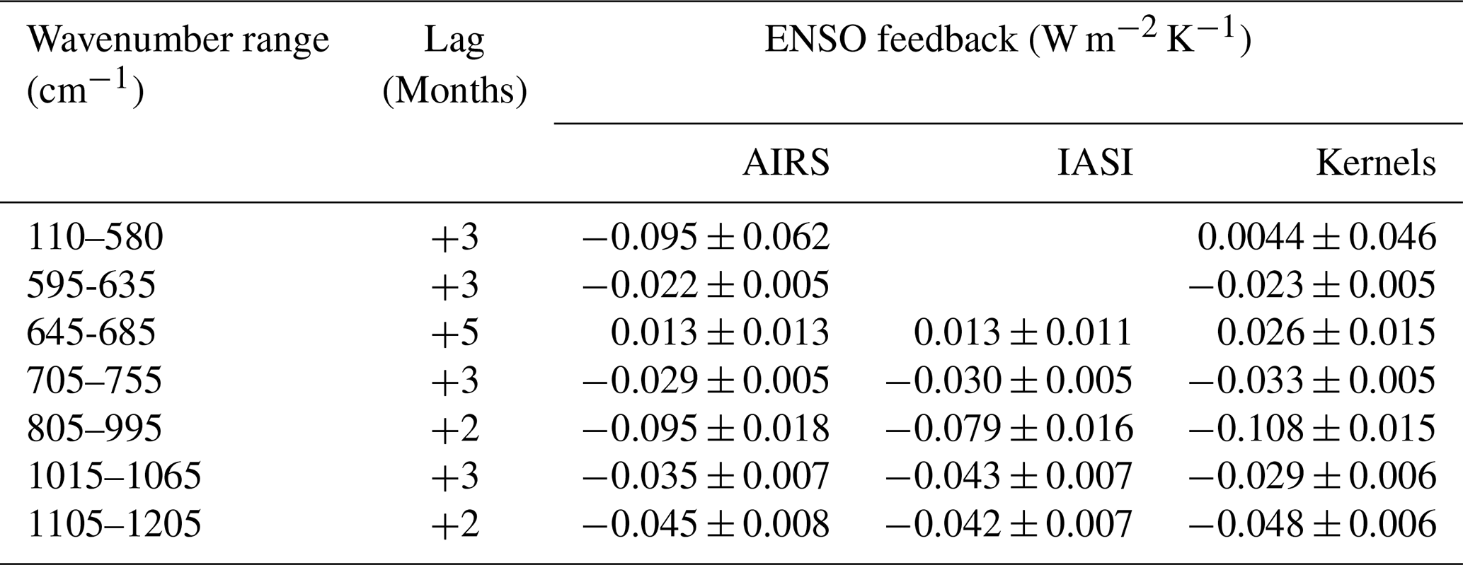
A summary of the ENSO spectral feedback for the spectral regions discussed above is provided by Table 2. It reports the value of the ENSO feedback integrated over each wavenumber interval, along with the lag at which the OLR response peaks in each spectral region.

AIRS and IASI spectral footprints are generally in a good agreement, showing the same main features. There are some differences in the magnitude of the response peak within the atmospheric window (∼ 800–1000 cm⁻¹), where the AIRS signal is slightly higher than that of IASI, but inside the uncertainty range (Table 2, fifth row and Fig. A3a). The opposite behavior is observed within the ozone absorption band (Table 2, sixth row and Fig. A3a), where a stronger signal is obtained for IASI. One factor to consider is the different overpass time of AIRS and IASI. This could partly explain the observed bias within the atmospheric window, where radiance is more sensitive to surface temperature (Whitburn et al., 2020). However, the different clear-sky scene selection could also play a role. Specifically, AIRS clear-sky fluxes are based on the collocated CERES measurements considered as clear-sky by the scene type information provided by the Moderate Resolution Imaging Spectroradiometer (MODIS), as described in Huang et al. (2008). We found that this strategy produced a more conservative cloud screening than that of IASI (not shown). This aspect will be more evident in Sect. 3.4, when we will examine the spatial pattern of the ENSO feedbacks.

Table 2 Total ENSO feedback associated to characteristic spectral regions obtained from AIRS, IASI and the reconstruction using spectral radiative kernels. The values reported correspond to the integral over the selected wavenumber intervals at the lag of the radiative response peak. The associated confidence interval (95 %) is reported.

3.3 Atmospheric drivers of the radiative response

The spectral fluxes of IASI and AIRS allowed us to study the total LW ENSO feedback associated with characteristic spectral regions and relate it to atmospheric and surface variables to which radiation is sensitive. Now, spectral radiative kernels are exploited to investigate the origin of the ENSO signal in more depth. Specifically, we address the individual radiative contribution associated with changes in surface and atmospheric temperature, water vapor and ozone. The corresponding surface and atmospheric Planck, water vapor and ozone ENSO feedbacks have been obtained by performing the same regression analysis that was performed on the IASI and AIRS observations. Results of the lagged regressions are plotted in Fig. 4.

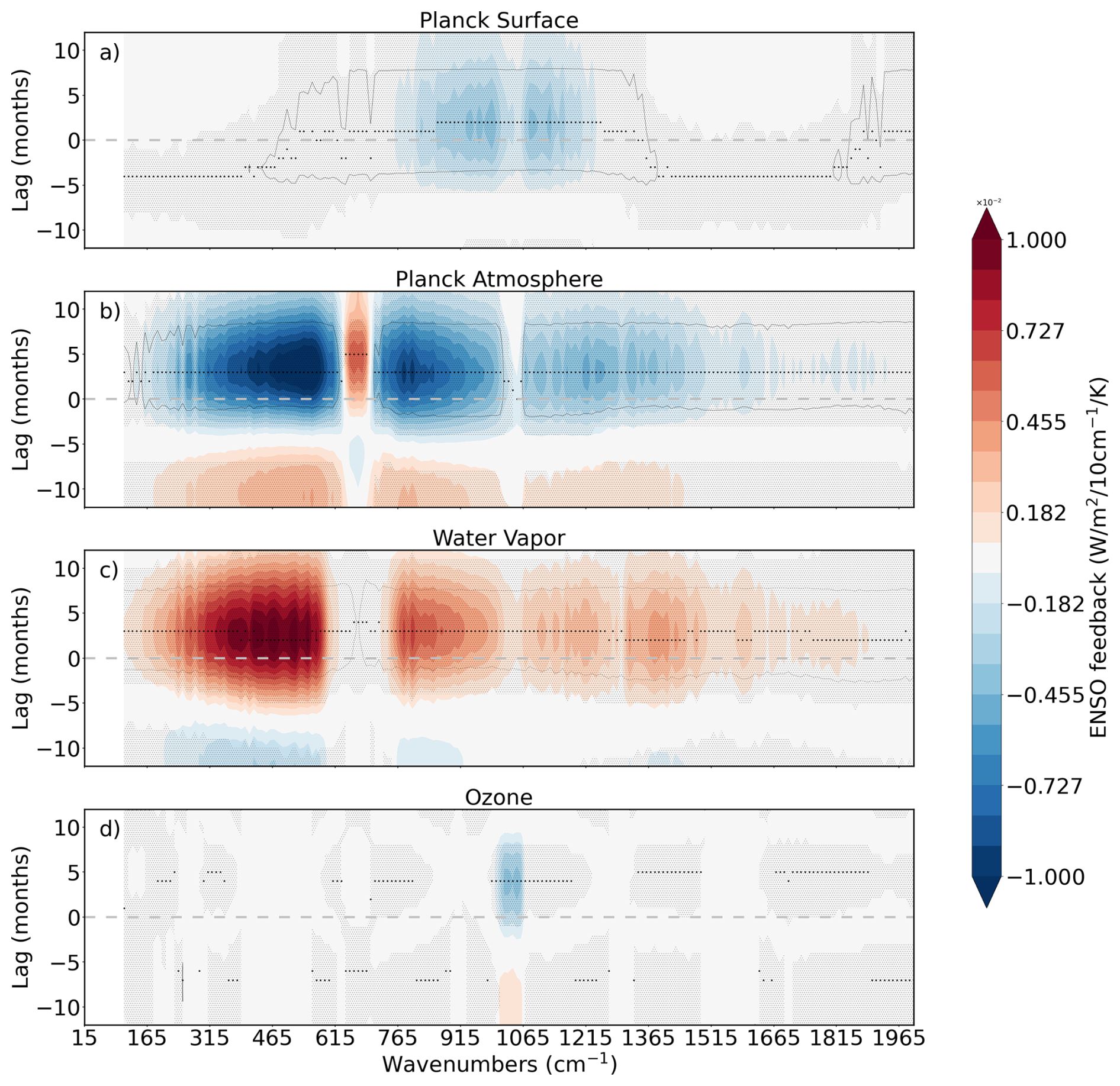
Figure 4 Lagged regressions between the tropical OLR anomaly driven by surface and atmospheric temperature (a, b), water vapor (c) and ozone (d) changes, and the Niño 3.4 index. Thinner black dots mark 95 % significance of the slopes, while thicker black dots mark the lag where the slope peaks at each wavenumber. Contour lines mark correlation values of 0.5. As above, the sign of the OLR has been inverted (negative feedback = positive OLR anomaly).

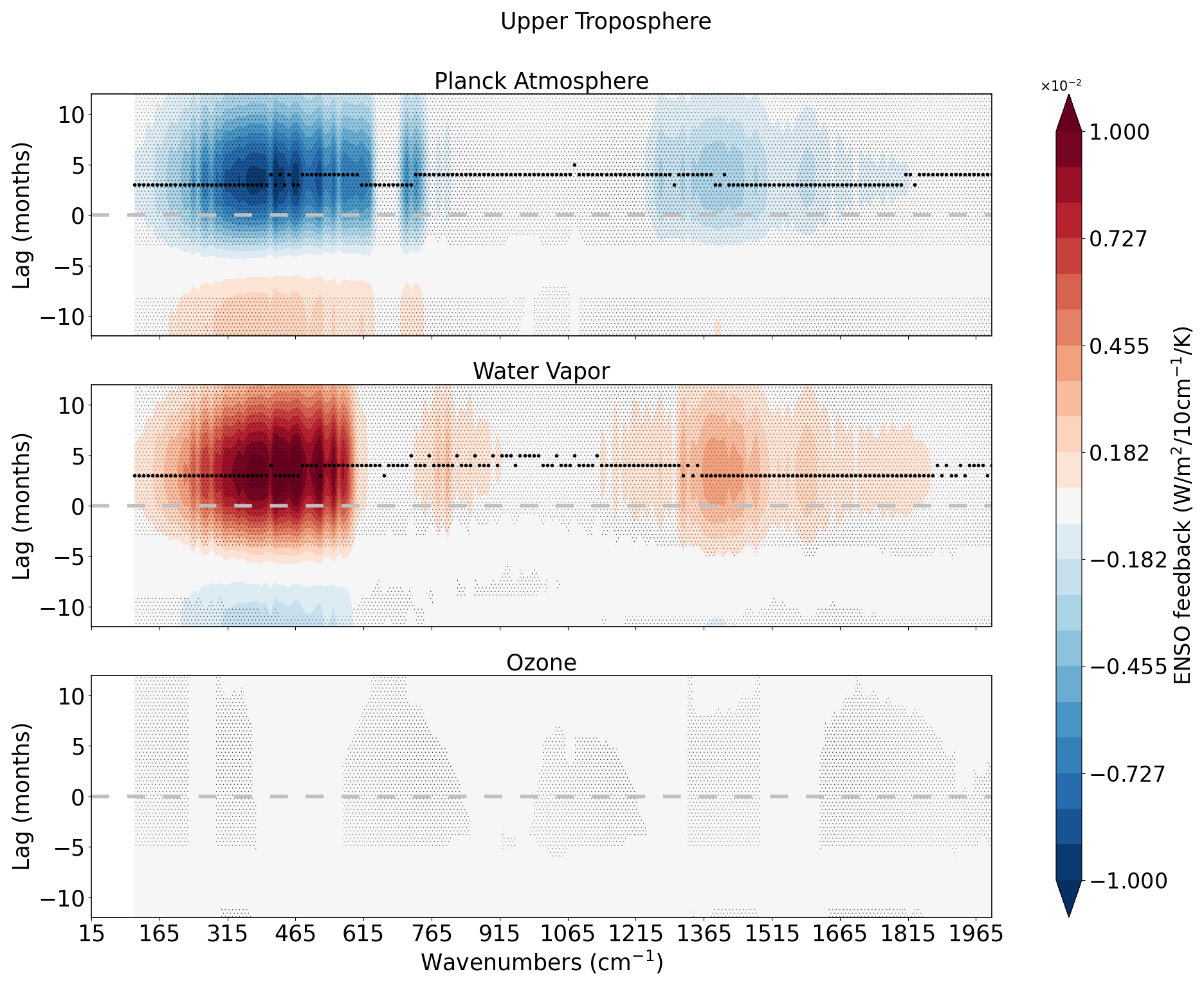
The Planck surface ENSO feedback (Fig. 4a) is negative and contributes to the TOA OLR only within the atmospheric windows, where the OLR is sensitive to the surface temperature. It peaks at a lag equal to 2 months across the two spectral ranges (∼ 800–1000 and ∼ 1100–1200 cm⁻¹). A negative feedback is also associated with the Planck atmospheric effect (Fig. 4b) below about 600 cm⁻¹, between 700–1000 cm⁻¹ and above 1100 cm⁻¹. Instead, the positive sign of the Planck atmospheric feedback between 645–700 cm⁻¹ (Fig. 4b) explains the positive ENSO feedback that characterizes also IASI and AIRS observations at the center of the carbon dioxide band (Fig. 3). In this spectral region the Planck atmospheric feedback peaks with a lag of 5 months, whereas over the remainder of the spectral range it peaks between 3 and 4 months lags. When the Planck atmospheric feedback is separated in a tropospheric and stratospheric contribution, with the tropical tropopause fixed at 100 hPa, it becomes evident that the positive feedback originates from the stratospheric temperature change (Fig. A5) and that the strong negative feedback within the FIR spectral region comes from the troposphere (Fig. A4), with the largest contribution from the upper troposphere (600–150 hPa) (Fig. A7). The Planck surface and atmospheric feedbacks are both negative, enhancing the OLR emission. Water vapor changes, instead, constitute the main positive ENSO feedback, acting to dampen the OLR emission. The water vapor feedback peaks with a lag of 3 months at all wavenumbers. As for the Planck atmosphere, the strongest signal occurs in the FIR spectral region, with the majority of the contribution coming from the upper troposphere (Fig. A7).

Given the strong ENSO feedback observed in correspondence of the ozone absorption band (Fig. 3), we isolated the ozone contribution to assess its specific impact. A negative feedback, peaking in the stratosphere (Fig. A5), is found between about 1010–1065 cm⁻¹, with a pick at 4-months lag. At the same wavenumbers and lags there is also a smaller positive feedback associated to the stratospheric temperature (Fig. A5), which, opposed to ozone, acts to reduce the OLR emission.

Finally, we reconstructed the total observed LW response summing the individual feedbacks calculated with kernels. The feedback sum is shown in Fig. 5, as a function of wavenumber and lag (panel a) and wavenumber only for the 2-months lag (panel b), along with its components. The main features of the AIRS and IASI clear-sky OLR response (Fig. 3) are present. The kernel regression analysis correctly reproduces the negative feedback within the two atmospheric windows and the wings of carbon dioxide absorption bands, as well as the positive feedback at the center of it. Except for the magnitude of the latter, which is overestimated by the feedback sum with respect to AIRS (Table 2, third row), both the amplitude and time-lag are well reproduced (Table 2). The difference between IASI total LW response and the feedback sum is reported in Fig. A3b. The main discrepancy arises in the spectral regions below 600 and above 1300 cm⁻¹: here AIRS fluxes indicate a negative feedback that peaks 3 months after ENSO, while the kernels reconstruction indicates a contribution close to zero at that lag (Table 2, first row) and a positive feedback that anticipates the ENSO peak (Fig. 5). A possible explanation for these two biases lies in the fact that ERA5 profiles used in the kernel reconstruction represent all-sky conditions. This leads to higher humidity content than in clear-sky profiles, causing an overestimation of the associated water vapor feedback and leading to the complete compensation between the atmospheric temperature and water vapor signal below 600 and above 1300 cm⁻¹ at positive lags.

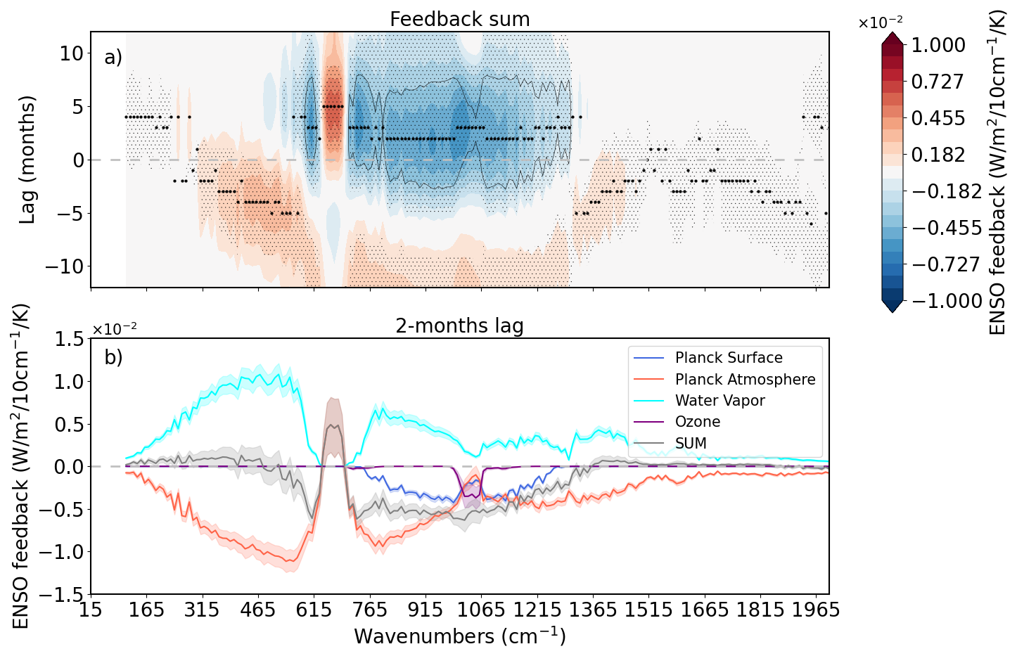
Figure 5 (a) Total OLR ENSO feedback reconstructed from the sum of individual feedback reported in Fig. 4. Thinner black dots mark 95 % significance of the slopes, while thicker black dots mark the lag where the slope peaks at each wavenumber. Gray contour lines mark correlation values of 0.5. (b) Same ENSO Planck surface (blue), Planck atmospheric (red), water vapor (cyan) and ozone (purple) feedback as Fig. 4, and feedback sum (gray) as panel (a), but plotted for the 2-months lag. Shades envelope the 95 % confidence interval. Contour lines mark correlation values of 0.5. As above, the sign of the OLR has been inverted (negative feedback = positive OLR anomaly).

In the next section (Sect. 3.4), the spatial pattern of the OLR response to ENSO is examined, which will help to trace the OLR response to specific regions of the tropical Pacific Ocean.

3.4 Spatial pattern of the longwave response to ENSO

We now examine the spatial pattern of the OLR response to ENSO across the tropics (30° S–30° N). Starting from the top of Fig. 6, the total OLR ENSO feedback obtained for IASI, AIRS and the kernel reconstruction is shown. The left column refers to the 900–910 cm⁻¹ interval, within the atmospheric window, where OLR is sensitive to surface temperature, but also to water vapor, that we want to assess and compare among the observed and reconstructed signal. The right column corresponds to the 1020–1030 cm⁻¹ interval, located within the ozone absorption band. Here, the OLR is mainly sensitive to surface temperature and ozone.

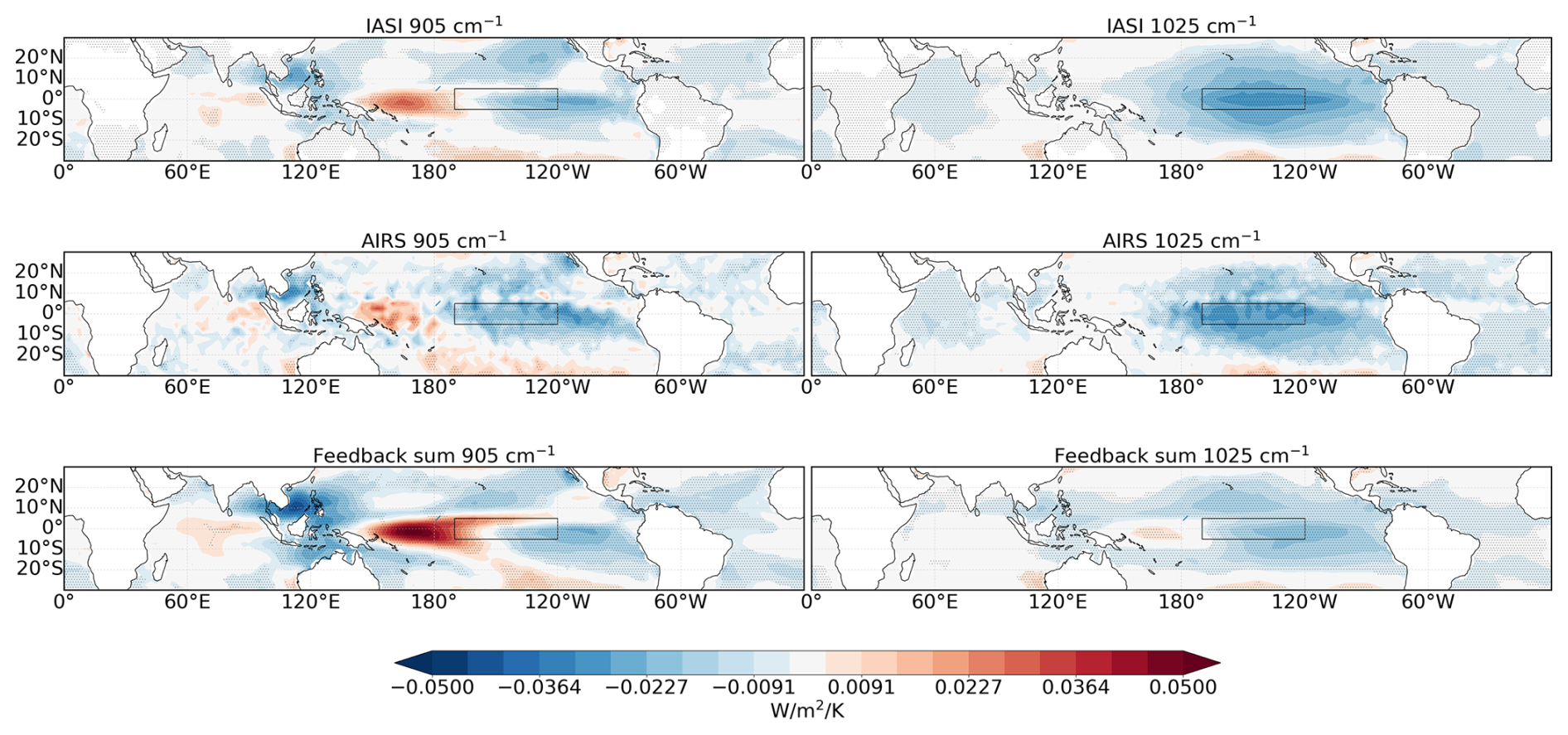
Figure 6 Spatial pattern of the total LW ENSO feedback of IASI (top maps), AIRS (central maps) and the kernels feedback sum (bottom maps), at 905 cm⁻¹ (left maps) and 1025 cm⁻¹ (right maps), for a lag equal to two months. Black dots mark regions where the regressions reach the 95 % significance level. The black rectangle highlights the Niño 3.4 region. As above, the sign of the OLR has been inverted (negative feedback = positive OLR anomaly).

At 905 cm⁻¹ the response, obtained from IASI and AIRS fluxes, shows a dipole within the tropical Pacific Ocean, in phase with the SST pattern typical of El-Niño conditions. Indeed, a positive ENSO feedback characterizes the western part of the basin, while a negative value is found in the central and eastern parts of the basin. Significant negative contributions are also found over the north-east subtropical region and over the Maritime Continent. The OLR response at 1025 cm⁻¹ is characterized by a negative feedback coming from the central and eastern part of the Pacific Ocean. Its magnitude is highest within the Niño 3.4 region (marked by a black box in Fig. 6), and decreases moving off the equator.

Although, there is a good agreement in the pattern obtained from IASI and AIRS data, as anticipated in Sect. 3.2, the impact of the clear-sky scene selection of AIRS observations is evident here. Specifically, AIRS shows a more scattered pattern with respect to IASI in the western and central tropical Pacific at 905 cm⁻¹.

Regarding the feedback sum, it correctly reproduces the response pattern at 905 cm⁻¹, but the magnitude of the positive feedback within the west Pacific is clearly overestimated. A similar discrepancy is also obtained for the reconstructed response at 1025 cm⁻¹, where the signal in the central and eastern regions is smaller in magnitude than observations and its peak is shifted eastward. The anomalous positive feedback can be attributed to the water vapor ENSO feedback, which shows a positive signal in the western and central parts of the Tropical Pacific Ocean at both 905 and 1025 cm⁻¹ (Fig. 7). These differences consolidate our hypothesis of an overestimation of the water vapor feedback, that would also overcompensate the Planck contribution below 600 cm⁻¹ and above 1300 cm⁻¹ in the kernel reconstruction (Sect. 3.3).

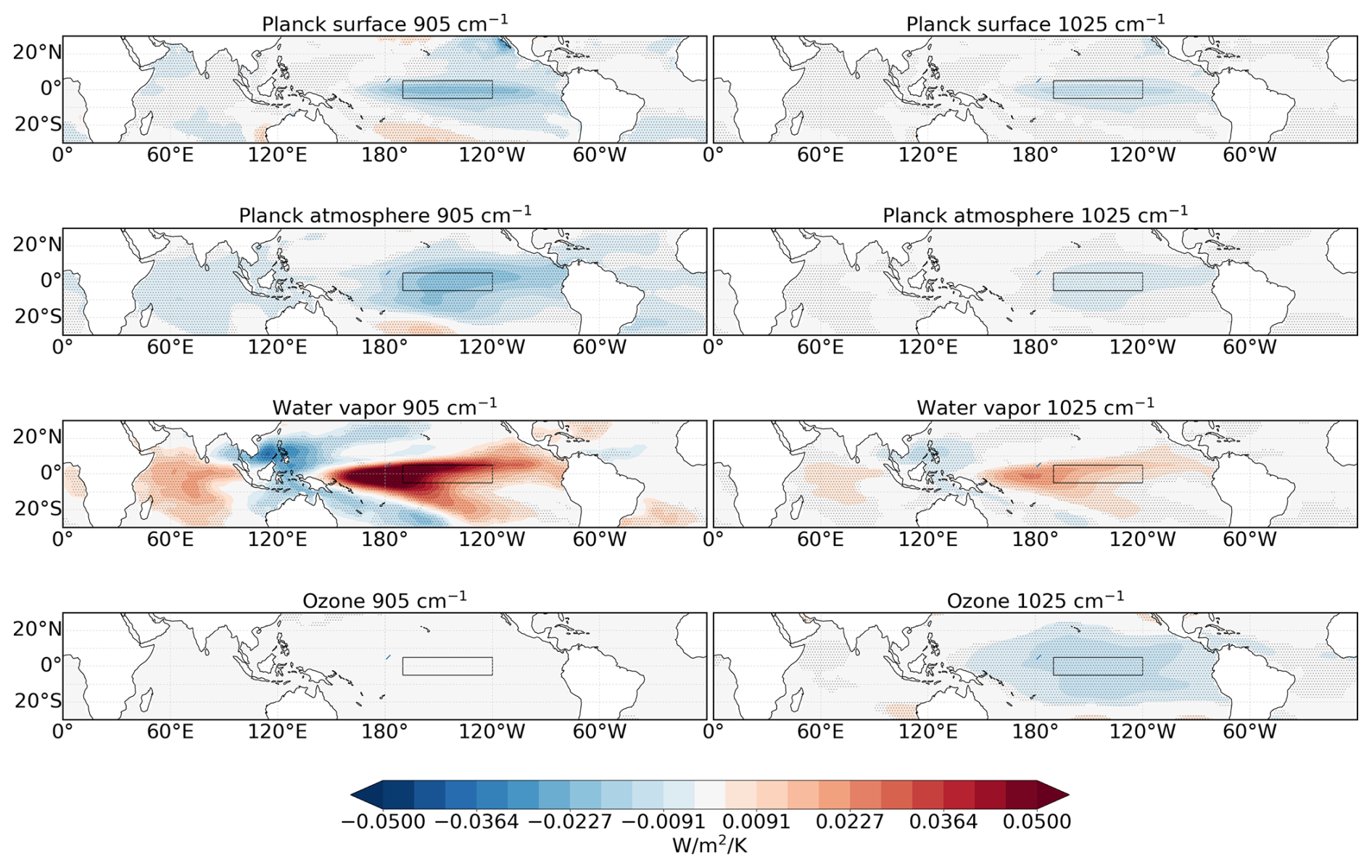
Figure 7 Spatial pattern of the Planck surface and atmosphere, water vapor and ozone ENSO feedback calculated using radiative kernels, at 905 cm⁻¹ (left maps) and 1025 cm⁻¹ (right maps), for a lag equal to two months. Black dots mark regions where the regressions reach the 95 % significance level. The black rectangle highlights the Niño 3.4 region. As above, the sign of the OLR has been inverted (negative feedback = positive OLR anomaly).

4 Discussion

The analysis reported in Sect. 3 highlighted some key features of the LW radiative response to ENSO that help to understand and constrain the main processes behind the variability of the tropical radiative budget.

The main effect of ENSO on the climate system is the anomalous SST pattern across the tropical Pacific Ocean, accompanied by a shift of the Walker Circulation (WC) (Bjerknes, 1966). During the positive El-Niño phase warmer SST anomalies characterize the eastern and central part of the basin, while cooler SSTs are found in the western part. The WC is shifted eastward, with an increase in convective activity over the central Pacific and a decrease over the west Pacific warm pool. The negative ENSO phase, La-Niña, brings to the opposite conditions, and it is accompanied by a strengthening of the WC.

In general agreement with Ceppi and Fueglistaler (2021), the clear-sky broadband OLR response suggests that ENSO activity during the time period considered resulted in an enhanced OLR emission at the TOA, whose peak lags ENSO by 2 months. The observed lag of the radiative response can be explained by the fact that ENSO-induced SST anomalies are not constrained to the Niño 3.4 region but migrate across the tropical Pacific ocean from the east, at the beginning of an El-Niño event, to the west, where positive anomalies persist up to five months after ENSO peak (Ceppi and Fueglistaler, 2021).

In this study, the combined use of spectrally resolved OLR measurements from the IASI and AIRS instruments, together with kernel analysis, allows the OLR response to ENSO to be disentangled, showing how the lag varies across different spectral ranges. Indeed, the spectrally resolved fluxes show that channels associated to the 2-months lag correspond to the atmospheric windows, whose radiance is mainly sensitive to the surface temperature. The response in other spectral regions is further lagged, from 3 months for regions sensitive to the upper troposphere to 5 months for the center of the CO₂ band, which is sensitive to the stratosphere, showing the impact of ENSO on the whole atmospheric column.

Although it does not directly emerge from IASI and AIRS observations, the spectral kernel analysis also shows that within the atmospheric windows the water vapor feedback counteracts the Planck surface feedback. It is important to note that water vapor concentration is affected by humidity changes arising from the anomalous atmospheric circulation during ENSO (Susskind et al., 2012). The effect of an increased water vapor concentration is to dampen the emission of OLR (positive feedback), absorbing most of the radiation emitted by the surface as a result of the increased SST (Raghuraman et al., 2019). At the same time the negative Planck atmospheric feedback contributes to the OLR emission at these wavenumbers as the main cooling mechanisms of the system, as pointed out by Huang et al. (2021) and Kolly and Huang (2018). The Planck atmospheric and water vapor feedback are dominant throughout the troposphere and counteract each other throughout the entire spectrum (Fig. 4b and c). However, according to the overall negative LW response obtained from IASI and AIRS observations, the Planck atmospheric feedback dominates, leading to an overall increase in OLR emission across the entire spectrum. We observe that they generally peak at the same 3-months lag, except in the FIR region between 400–600 cm⁻¹, where the temperature peaks at 3 months while the water vapor peaks at 2-months lag (Fig. 3).

When considering the ENSO-driven OLR response under clear-sky conditions, the main radiative feedbacks are those induced by temperature and water vapor changes. We obtain a value of −0.94 ± 0.05 W m⁻² K⁻¹ for the broadband temperature LW ENSO feedback (sum of the Planck surface and atmospheric feedback, integrated along the spectral dimension) at the 3-months lag, which shows a fairly good agreement with that obtained by Kolly and Huang (2018) (see their Fig. 3). While our broadband water vapor LW feedback, at the same time lag, is of 0.69 ± 0.07 W m⁻² K⁻¹, which is larger than that of Kolly and Huang (2018), which is around 0.5 W m⁻² K⁻¹ (see Fig. 3 of Kolly and Huang (2018)). In addition to the different time period of the analysis, this can be explained both by the different set of radiative kernels used for the study, as well as the reanalysis product employed for the calculation of the radiative perturbations (ERA5 in this work and ERA-Interim in the work of Kolly and Huang, 2018). These results are also broadly consistent with the analysis carried out by Raghuraman et al. (2019) (see their Table 3), although the different framework hampers a more quantitative comparison.

In addition, we found a significant negative feedback associated to ozone changes. Together with the positive Planck atmospheric feedback observed at the center of the carbon dioxide absorption band, this reveals the ENSO-related stratospheric signal (Zeng and Pyle, 2005; Randel et al., 2009; Calvo et al., 2008; Manzini, 2009; Konopka et al., 2016; Manatsa and Mukwada, 2017; Garfinkel et al., 2018). According to Domeisen et al. (2019), a reduction in ozone concentration near and above the tropopause is observed as a result of the anomalous upwelling during El-Niño, which cause an increase of ozone-poor air in the central and eastern tropical Pacific. This agrees with the spatial patterns reported in Fig. 7, which show that at 1025 cm⁻¹ the ozone feedback characterizes these regions. Our analysis adds evidence to the attribution of IASI radiance trends in the ozone band in Whitburn et al. (2021) to ENSO-related ozone changes. In addition to composition changes, El-Niño also affects the stratospheric temperature. Specifically, an opposite response is observed compared to the troposphere. The ENSO impact on stratospheric temperature is the result of the upward propagation of Rossby waves forced by El-Niño and the strengthening of the Brewer Dobson Circulation (Domeisen et al., 2019). The stratospheric temperature decrease related to ENSO can explain the coherent decrease in TOA OLR emission observed at the center of the carbon dioxide absorption band (Figs. 3 and A5). Although a stratospheric signal is also involved, a decrease in the OLR is not observed in the ozone band, since the ozone concentration is also co-varying with ENSO near and above the tropopause, reversing the overall signal there. These findings confirm that the ENSO stratospheric signal plays an important role in shaping the LW radiative response peak.

5 Conclusions

In this work, we used spectrally resolved observation of the OLR to isolate and constrain the main processes controlling the inter-annual variability of the tropical energy budget. We focused on ENSO as the main driver of inter-annual radiative perturbations to the tropical OLR. Results further consolidate the potential of satellite-based spectrally-resolved measurements of the OLR to constrain the fast inter-annual feedbacks and isolate the processes driving them.

We recall here the main results of the study:

• The lagged regression analysis based on the spectrally-integrated tropical OLR from AIRS is largely consistent with CERES, with a slight delay of AIRS, likely due to the spatial sampling strategy used for the radiance to flux conversion. IASI and AIRS agree very well when integrated on the same spectral range, supporting the consistence among different data products.

• Further insight into the OLR response to ENSO is enabled by the spectral analysis:

  • –

    The lag of the response is spectrally dependent, with channels sensitive to lower atmospheric layers peaking earlier than channels sensitive to the stratosphere.

  • –

    The peak of the radiative response is found between ∼ 1000–1065 cm⁻¹ in correspondence with the ozone absorption band and follows ENSO by three months.

• The spectral kernel analysis gives additional information on the processes driving the observed signal:

  • –

    The Planck surface feedback (peaking at two-months lag) and the Planck atmosphere feedback (three-months lag) are responsible for the negative LW feedback observed throughout the spectrum, that causes an increase in OLR following ENSO. The only positive feedback, which acts to decrease the OLR, is the water vapor feedback, that also peaks at three-months lag.

  • –

    The response at the center of the carbon dioxide absorption band together with the ozone is likely the result of ENSO induced changes to the stratospheric composition and temperature, which are important for the LW radiative response peak.

  • –

    The sum of the Planck surface, atmosphere, water vapor and ozone feedback generally reproduces the observed signal, though with some differences. In particular, the water vapor feedback perfectly balances the Planck atmosphere feedback, while the observations show that the temperature response prevails. These discrepancies may be caused by an over-estimation of the water vapor response due to the fact that the ERA5 temperature/humidity fields refer to all-sky conditions.

In the FIR spectral region, both the water vapor and temperature ENSO feedbacks are higher, but to date we could only rely on simulated spectral fluxes at these wavenumbers. In this regard, an important contribution will be provided by the future Far-infrared Outgoing Understanding and Monitoring (FORUM) mission, the selected Earth Explore-9 (EE-9) of the European Space Agency (ESA) (Palchetti et al., 2020), that will close this observational gap, allowing to assess the role of this critical region for the inter-annual and forced climate feedbacks.

This work sets the basis for a future investigation of ENSO-induced variability of the OLR as simulated by climate models. The spectral dimension will allow to disentangle the various processes contributing to ENSO OLR response avoiding compensating errors that may arise from the use of broadband OLR. In an upcoming study, we plan to apply this diagnostic to evaluate the climate models participating in the CMIP6. This could improve our understanding of how models reproduce the coupled atmosphere-ocean dynamics that drive the ENSO response.

Appendix A

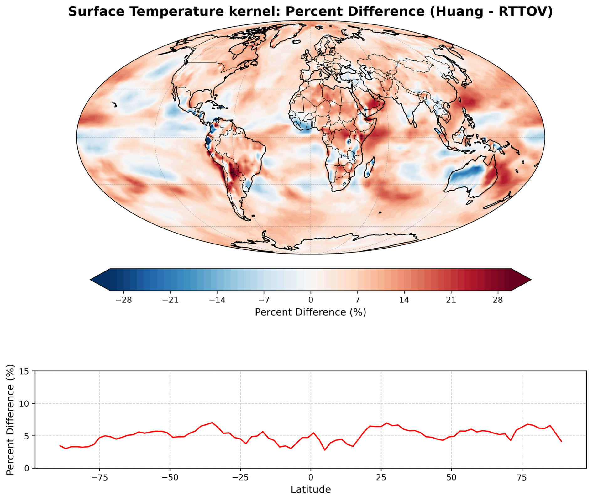
Figure A1 Differences between clear-sky surface temperature radiative kernels used for this work (RTTOV) (Della Fera et al., 2025) respect to radiative kernels computed by Huang and Huang (2023) (Huang). Spatial distribution of the percentage differences (upper map) and over the longitudinal mean (lower panel).

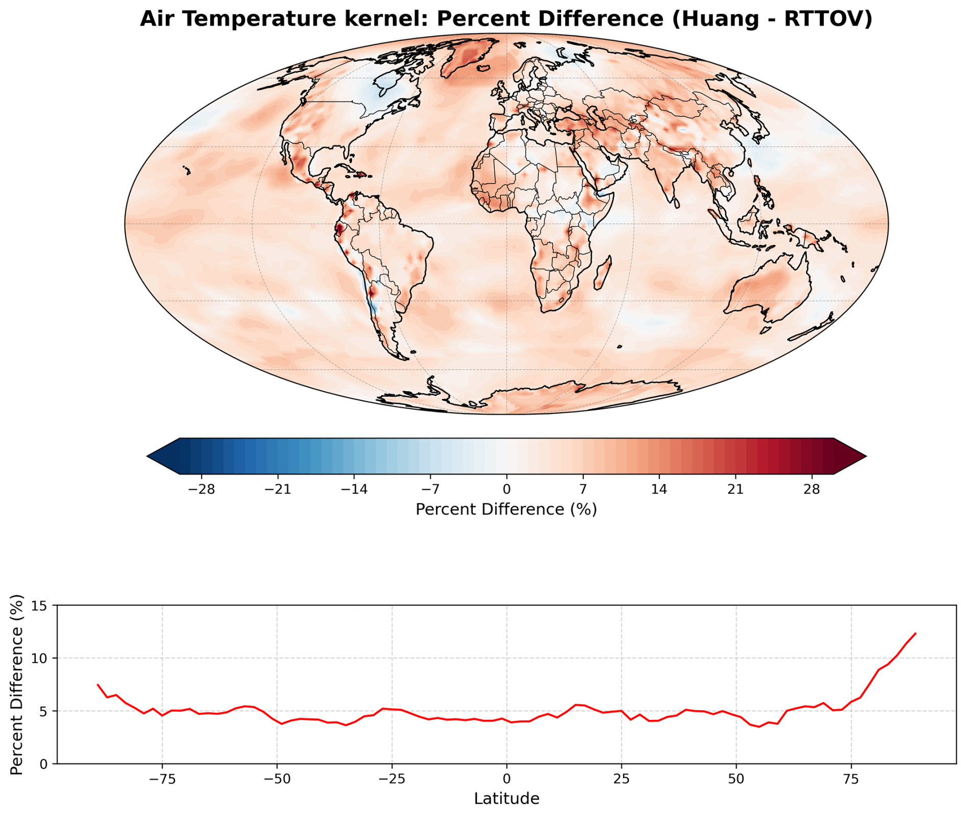
Figure A2 Same as Fig. A1 but for air temperature radiative kernel.

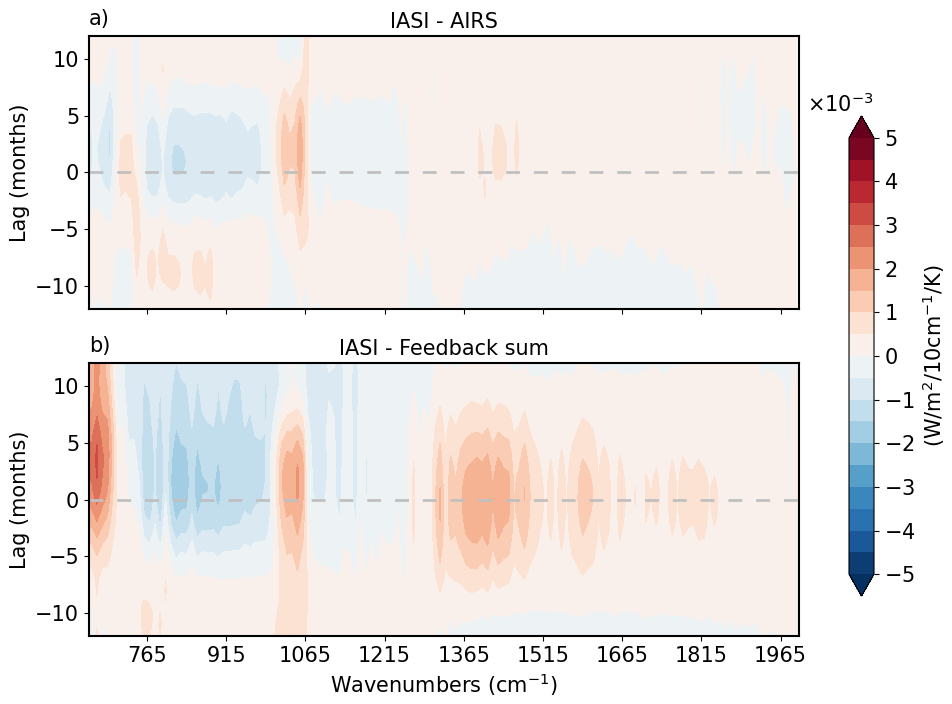
Figure A3 Differences in the tropical mean lagged regressions between the OLR and the Niño 3.4 index, obtained using IASI and AIRS observations (a) and IASI and the reconstructed signal (Feedback sum) (b).

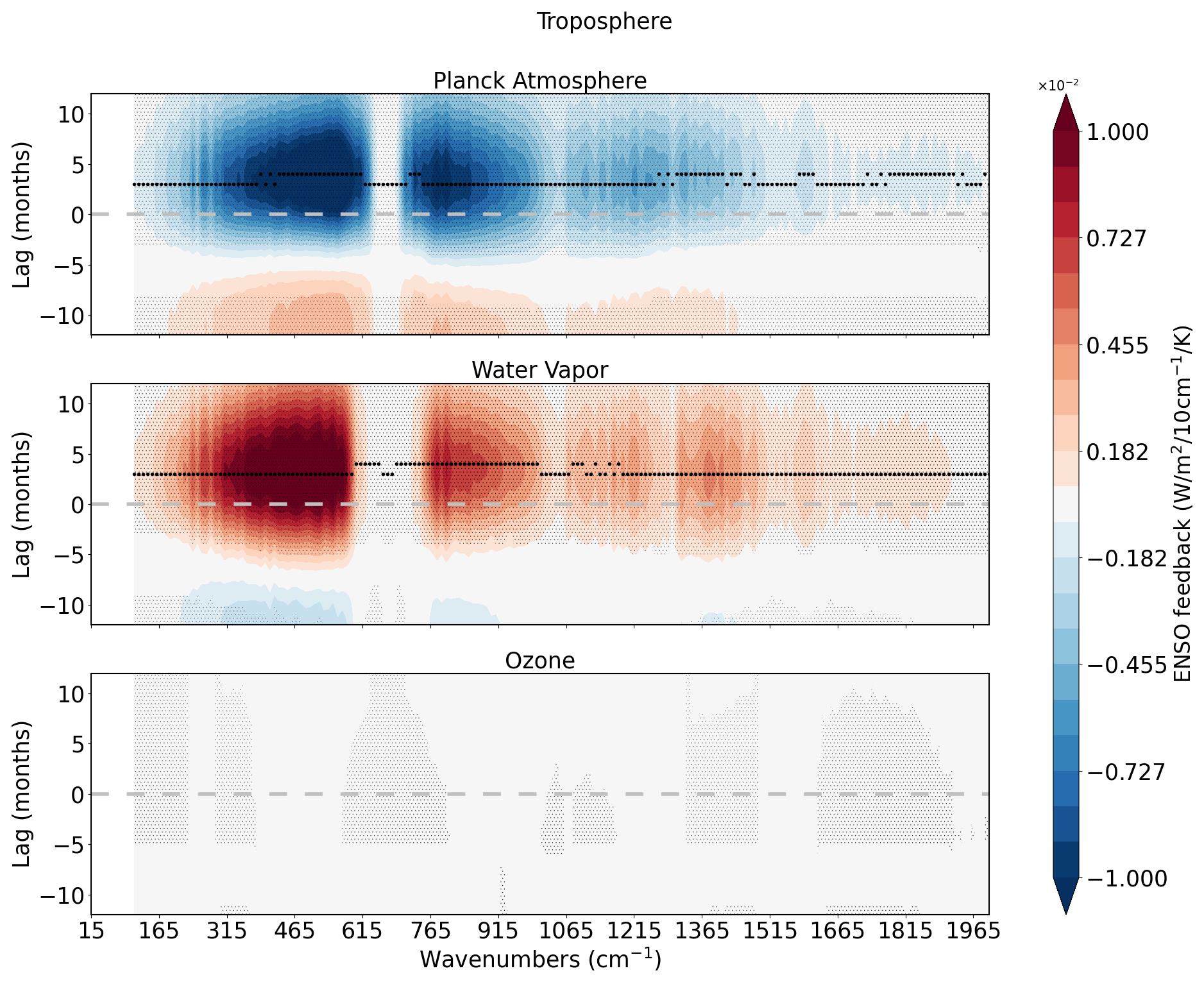
Figure A4 Lagged regressions between the tropospheric OLR anomaly driven by atmospheric temperature, water vapor and ozone changes, and the Niño 3.4 index. The tropical tropopause is set at 100 hPa. Thinner black dots mark 95 % significance of the slopes, while thicker black dots mark the lag where the slope peaks at each wavenumber.

Figure A5 Same as Fig. A4, but for radiative changes within the stratosphere (150–10 hPa).

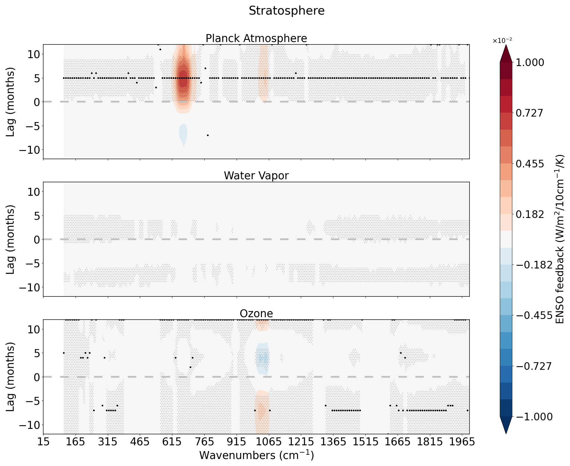
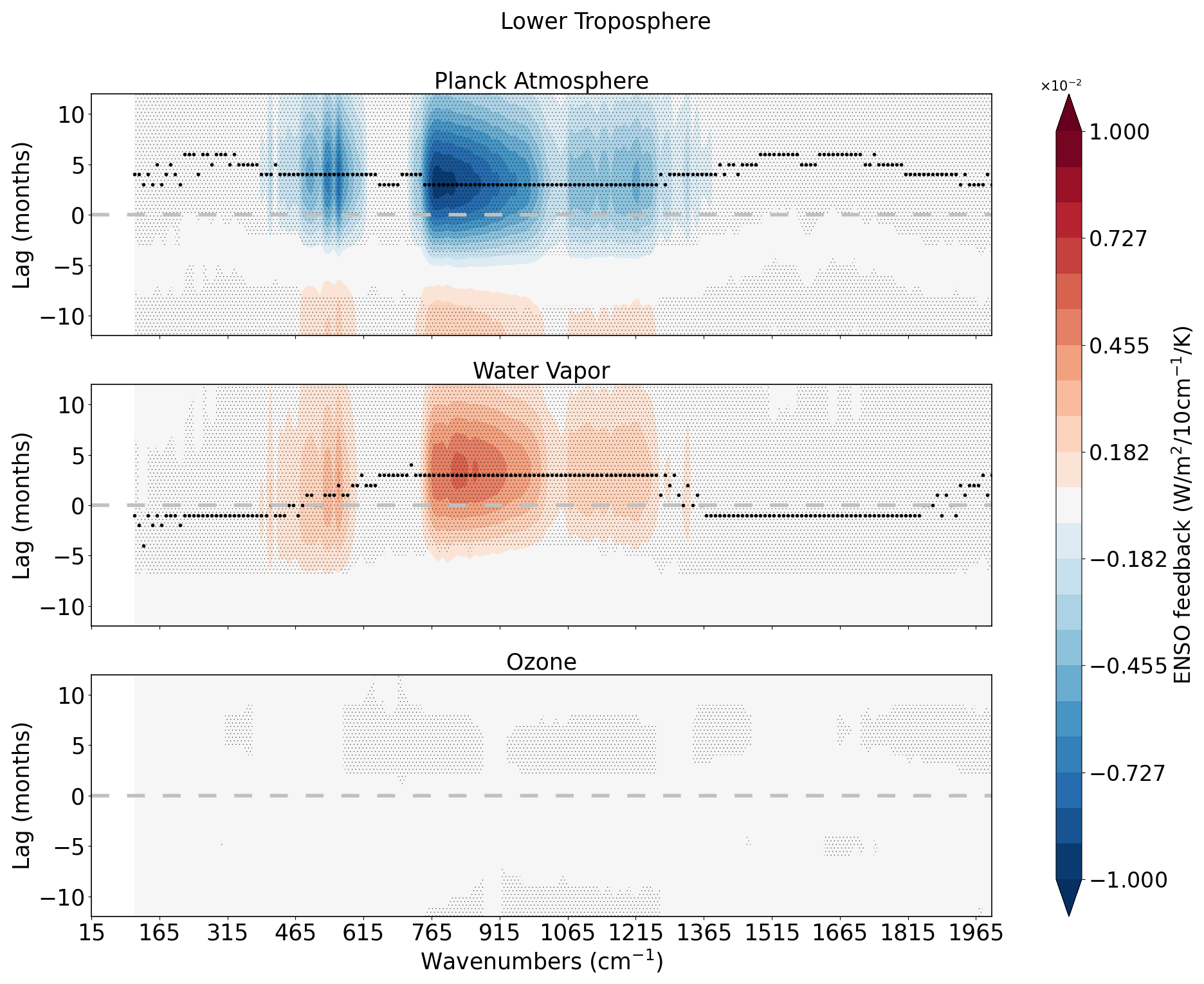
Figure A6 Same as Fig. A4, but for radiative changes within the lower troposphere (1000–600 hPa).

Figure A7 Same as Fig. A4, but for radiative changes within the upper troposphere (600–150 hPa).