Drivers and implications of declining fossil fuel CO₂ concentrations in Chinese cities revealed by radiocarbon measurements

China's clean air policies have successfully mitigated fossil fuel CO₂ (CO_2ff or C_ff) emissions in bottom-up inventories since 2013. Yet, evidence from top-down measurements and their underlying drivers remains limited. Here, we quantify C_ff concentrations and fuel-specific contributions using atmospheric Δ(¹⁴CO₂) and δ(¹³CO₂) measurements across representative Chinese cities. We found regional differences in C_ff and co-emission characteristics: megacities like Guangzhou show an indicative inter-period decrease in wintertime C_ff concentrations, of roughly 56 %–64 % lower in 2022 than in 2010 in afternoon-equivalent terms, while smaller cities have yet to demonstrate comparable decreases. These changes are consistent with a 23 % reduction in coal use, a 17 % increase in the natural-gas contribution (evidenced by stable isotope analysis), and improved combustion efficiency (indicated by a 63 % decline in $R_{\mathrm{CO}/{\mathrm{CO}}_{\mathrm{2}\mathrm{ff}}}$ ratios). Notably, the 24 years observational record (1998–2022) shows steeper declines in urban $R_{\mathrm{CO}/{\mathrm{CO}}_{\mathrm{2}\mathrm{ff}}}$ ratios than inventory estimates, suggesting current emission inventories may underestimate combustion efficiency improvements and CO emission reductions relative to C_ff mitigations. These findings are consistent with progress toward mitigating C_ff and co-emitted CO in major Chinese cities. They also underscore how coal-to-gas transitions and technological upgrades simultaneously advance air quality and climate goals. Importantly, our results highlight the critical need to integrate top-down observational frameworks (e.g. radiocarbon measurements) with traditional inventories to better capture rapid, policy-driven emission changes and inform future co-benefit optimization strategies.

1 Introduction

As the world's largest energy consumer, China's heavy reliance on fossil fuels has resulted in severe air pollution and substantial fossil fuel CO₂ (CO_2ff or C_ff) emissions, accounting for 31 % of global fossil CO₂ emissions in 2022 (Friedlingstein et al., 2023a). These emissions pose critical threats to public health and ecological stability. In response, China has enacted progressive policies including the 2013 Clean Air Action Plan (Zheng et al., 2018; Zhang et al., 2019), 2018 Blue Sky Defense Battle, and 2022 Pollution-Carbon Synergy Plan, achieving co-benefits in air quality improvement and C_ff mitigation as quantified through bottom-up inventories like Multi-resolution Emission Inventory for China (MEIC) (Shi et al., 2022). However, the effectiveness of these policies in reducing atmospheric C_ff concentrations, and the underlying drivers of these reductions, remains unverified and unexplored through top-down observational approaches, creating a critical knowledge gap in climate policy assessment.

Bottom-up inventories and top-down measurements are approaches commonly used to determine atmospheric C_ff emissions, but each has inherent limitations that can affect accuracy and reliability. Although bottom-up inventories are available at increasingly higher spatiotemporal resolution (Han et al., 2020), they are time-consuming to compile and update promptly, often lack quantitative estimation of uncertainty (Crippa et al., 2019), and frequently debated in attributing emissions to specific sources (Gurney et al., 2021). In contrast, top-down studies encompass all existing sources within a geographic region but struggle to achieve accurate partitioning of the fossil fuel and biospheric CO₂ contributions. This methodological impasse can be resolved by ¹⁴C analysis, which exploits the unique ¹⁴C-depletion signature of C_ff compared to contemporary biogenic sources (Levin et al., 2003; Turnbull et al., 2006), enabling unambiguous fossil fuel emission quantification.

Urban areas, occupying merely 3 % of global land yet responsible for 75 % of global C_ff emissions (reaching 80 % in China) (Dhakal, 2009; Duren and Miller, 2012), represent strategic priorities for emission mitigation. Recent advances in analytical tools can help identify key drivers of urban C_ff reductions. δ(¹³CO₂) signatures successfully distinguished coal, oil, and natural gas contributions in cities like Beijing and Xi'an (Wang et al., 2022b), while $\mathrm{\Delta }\mathrm{CO}/C_{\mathrm{ff}}$ (ΔCO denotes the difference between observed and background values; $\mathrm{\Delta }\mathrm{CO}={\mathrm{CO}}_{\text{obs}}-{\mathrm{CO}}_{\text{bg}}$) ratios tracked combustion efficiency variations across national (China, South Korea) and urban (Paris, Heidelberg) scales (Turnbull et al., 2011; Lee et al., 2020; Lopez et al., 2013; Rosendahl, 2022). To address the research gaps mentioned above, we performed spatiotemporal mapping of 2022 C_ff concentrations across representative Chinese cities using dual-carbon isotope constraints (Δ(¹⁴CO₂)+δ(¹³CO₂)) for fuel-specific source attribution. By integrating multi-source inventories with extended $\mathrm{\Delta }\mathrm{CO}/C_{\mathrm{ff}}$ observations through 2022, we developed a robust framework for top-down verification of policy-driven emission reductions. Our methodology not only quantifies C_ff concentration decreases but also identifies the key mechanisms behind these reductions, offering critical insights for refining climate mitigation strategies and supporting sustainable urban development.

2 Data and methods

2.1 Study area and sample collection

We selected representative Chinese cities of varied population sizes for this study: Guangzhou, Shenzhen, and Beijing for megacities (urban permanent resident populations>10 million), Xi'an for supercities (5–10 million), Zhanjiang for large cities (1–5 million), and Shaoguan for medium and small cities (<1 million), which is retrieved from the Tabulation on 2020 China Population Census by Office of the Leading Group of the State Council for the Seventh National Population Census, 2022). Since we could obtain results in Beijing and Xi'an from previous studies, we conducted field sampling in the four cities in Guangdong Province, China (Fig. 1). Guangdong Province is located south of the Nanling Mountains and on the coast of the South China Sea, lying within subtropical and tropical low-latitude regions. The area experiences a prevailing southeast monsoon from the ocean during summer and a northeast monsoon from the continent during winter. The four cities in Guangdong Province differ in terms of area, population, gross domestic product (GDP), C_ff inventory emissions, population density, topographic elevation, and land use/land cover. Guangzhou and Shenzhen represent two of China's seven megacities – approximately 45 exist globally – within the Pearl River Delta (PRD), the world's largest urban agglomeration (Taubenböck et al., 2019). Guangzhou, the capital of Guangdong Province, has a population of 18.7 million, GDP of 2884 billion Yuan, and built-up area covering 35.2 %. Shenzhen, a high-tech hub transformed by post-1978 reforms, hosts 17.7 million people with GDP reaching 3239 billion Yuan and 53.8 % built-up coverage. In contrast, Zhanjiang (large city) and Shaoguan (medium and small city) have smaller populations – 7.0 million and 2.9 million respectively – and lower GDPs of 371.3 billion Yuan and 156.4 billion Yuan. Zhanjiang features extensive cultivated land (31.7 %) and coastal ports (Zhanjiang Municipal Bureau of Statistics, 2025), while Shaoguan is distinguished by 74.5 % forest coverage (Shaoguan Municipal Bureau of Statistics, 2024).

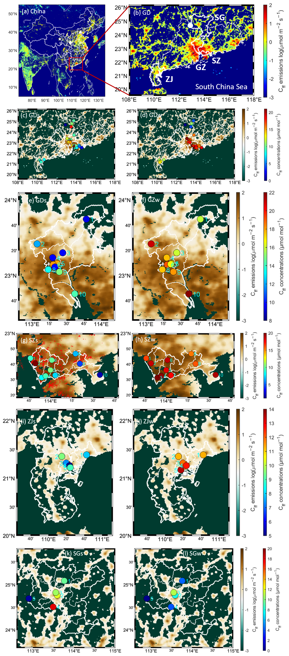
Figure 1 Locations of sampling sites and spatial distribution of C_ff concentrations during summer (s) and winter (w) in (c, d, GD) Guangdong Province and the cities of (e, f, GZ) Guangzhou, (g, h, SZ) Shenzhen, (i, j, ZJ) Zhanjiang, and (k, l, SG) Shaoguan. White-filled symbols denote Beijing (▴), Xi'an (⧫), and Waliguan (⋆) in (a); Nanling (•) in (b); Shenzhen Airport (▸) in (g); and Zhanjiang Port (▪) in (j). Shenzhen's industrial land use (https://download.geofabrik.de/asia/china.html, last access: 11 November 2025) is shown as red in (g), with the spatial distribution of all industrial enterprises and CO₂-emitting facilities documented in Li et al. (2025a). Colored circles in (c)–(l) represent the observations, while the shading indicates the C_ff inventory emissions from the Open-source Data Inventory for Anthropogenic CO₂ (ODIAC) (Oda and Maksyutov, 2024) in August and December with 1 km×1 km grid spacing. White lines indicate boundaries of cities in Guangdong Province (c, d), and boundaries of districts in the four cities (e–l). In (c), (d), bold white lines indicate boundaries of nine cities of the Pearl River Delta. The left color bar represents the C_ff inventory emissions, while the right color bar represents the C_ff observations.

We collected 240 air samples from 30 sites during summer (28 July–30 August 2022) and winter (12 December 2022–6 January 2023) campaigns, with weekly sampling in both periods. Because atmospheric transport variability can influence observed C_ff signals, we evaluated the meteorological representativeness of the sampling months using ERA5 diagnostics and trajectory analyses. Specifically, we assessed whether the August and December 2022 flask measurements were representative of typical summer and winter transport conditions. Standardized anomalies ($z=(x_{\text{target}}-{\mathit{\mu }}_{\text{season}})/{\mathit{\sigma }}_{\text{season}})$ were calculated for five ERA5 meteorological variables: 10 m eastward wind (U10), 10 m northward wind (V10), 2 m air temperature (T2M), surface pressure (SP), and planetary boundary-layer height (PBLH). Each target month was compared against (i) the concurrent 2022 seasonal background (June–July–August, JJA; December–January–February, DJF) and (ii) the 2010–2021 seasonal climatology. The choice of 2010 as the starting year ensures consistency with the earlier dataset from 2010, which is directly compared in this study. A month was considered “typical” when $|z\le \mathrm{1}$ and its dominant wind direction fell within the canonical summer (90–225°) or winter (0–45°) monsoon sectors.

The locations and details of these sampling sites are shown in Fig. 1 and summarized in Table A1. Ten sampling sites were located in Guangzhou (GZ1–GZ10), ranging from urban downtown to suburban areas, selected based on spatial gradients of C_ff emissions derived from the Open-source Data Inventory for Anthropogenic CO₂ (ODIAC) (Oda and Maksyutov, 2011; Oda and Maksyutov, 2024). Another 10 sampling sites were distributed uniformly throughout Shenzhen (SZ1–SZ10). In Zhanjiang (ZJ1–ZJ5) and Shaoguan (SG1–SG5), five sampling sites were selected in each city, primarily in urban areas, and distributed according to the first and second most dominant wind directions. These sites are located on the tower or on the roof of the building with 10–12 m extendable masts and are chosen to be free from any modifying effects of surrounding skyscrapers. Most of our sampling sites are generally no more than 300 m from the nearest air quality monitoring station. The sampling height is usually kept above 30 m above the ground level to avoid the influence of local sources. We assume that the measurements at the sampling sites in Guangzhou and Shenzhen are statistically sufficient to assess the whole cities, while those in Zhanjiang and Shaoguan are sufficient to assess the urban areas. Air sampling occurred between 13:00 and 17:00 LT (local time), coinciding with the deepest planetary boundary layer and well-mixed atmospheric conditions. Post-filtration samples were transferred into pre-evacuated/flushed 3 L borosilicate flasks using 12 V micro-diaphragm pumps. These delivered a flow rate of 6 L min⁻¹ at 25 °C and 101.3 kPa, with pressurization to 172.4–206.8 kPa. The duration of the sampling was approximately 15–20 min in total.

2.2 Measurement of atmospheric CO₂ and δ(¹³C)

Whole-air samples were dried using magnesium perchlorate at a constant flow rate of 25 mL min⁻¹, controlled by a mass flow controller. The CO₂ concentrations and δ(¹³C) values were then measured using a Picarro G2201-i high-precision carbon isotope analyzer (Picarro, Inc., Santa Clara, CA, USA) with cavity ring-down spectroscopy. Each sample was measured for 10 min, and only data from the final 5 min were used to calculate the average CO₂ concentration and δ(¹³C) value. Calibration for the CO₂ concentrations and the δ(¹³C) values was performed using the method described by Wen et al. (2013) with three standards: (a) (409.47±0.02) ppm (µmol mol⁻¹; similar hereafter), $(-\mathrm{8.717}\pm \mathrm{0.013})\mathrm{‰}$; (b) $(\mathrm{447.78}\pm \mathrm{0.01})\mathrm{\mu }\mathrm{mol}{\mathrm{mol}}^{-\mathrm{1}}$, $(-\mathrm{9.759}\pm \mathrm{0.006})\mathrm{‰}$; and (c) $(\mathrm{503.65}\pm \mathrm{0.01})\mathrm{\mu }\mathrm{mol}{\mathrm{mol}}^{-\mathrm{1}}$, $(-\mathrm{11.456}\pm \mathrm{0.004})\mathrm{‰}$, obtained from the Chinese Academy of Meteorological Sciences. The CO₂ concentrations of the standards are traceable to the X2019 standard scale maintained by the Central Calibration Laboratory of the World Meteorological Organization, and the δ(¹³C) values are traceable to the stable isotope laboratory of the Institute of Arctic and Alpine Research based on the NBS-19 and NBS-20 standards. The δ¹³C values were reported relative to the international Vienna Pee Dee Belemnite standard (Coplen, 1996). The precision was better than 0.2 µmol mol⁻¹ for CO₂ concentrations and 0.1 ‰ for δ(¹³C) values.

2.3 Measurement of atmospheric Δ(¹⁴C)

The residual air samples were transferred into a vacuum system at a flow rate of 300 mL min⁻¹. It was then first passed through a cold trap consisting of dry ice and ethanol slurry to freeze out water, followed by passage through a liquid nitrogen cold trap (−196 °C) to freeze down the CO₂ (Xu et al., 2007). The extracted and purified CO₂ was converted into graphite using the hydrogen reduction method. The graphite was then pressed into an aluminum holder for ¹⁴C measurements using an NEC 0.5MV 1.5SDH-2 accelerator mass spectrometer (AMS, National Electrostatics Corporation, USA) (Zhu et al., 2015). Each measurement wheel typically comprises 13 primary standards (oxalic acid II), 13 sary standards (IAEA-C7), 13 solid process blanks (p-phthalic acid), 6 gas process blanks (¹⁴C-free CO₂ in synthetic air from a cylinder), and some authentic air samples. The results are presented as Δ(¹⁴C), which is the per mill (‰) deviation from the absolute radiocarbon reference standard, corrected by fractionation and decay Stuiver and Polach, 1977). We analyzed 17 pairs of parallel air samples to evaluate the quality control and assurance of the entire sampling and laboratory analysis process, including sampling, extraction, graphitization, and AMS measurement. The AMS measurement uncertainty and the average deviation are (2.1±0.3) ‰ and (0.2±2.9) ‰, respectively (see Fig. A1). We thus specify a one-sigma measurement uncertainty of 2.9 ‰ for Δ(¹⁴C) based on these repeat measurements of air samples.

2.4 C_ff concentration estimation (incorporated biomass burning emissions)

Recently added atmospheric CO₂ (CO_2obs or C_obs) is thought to consist of background CO₂ (CO_2bg or C_bg) and excess CO₂ (CO_2xs or C_xs). The C_xs mainly includes C_ff and biogenic CO₂ (CO_2bio or C_bio). The corresponding Δ(¹⁴C) values are expressed as Δ_obs, Δ_bg, Δ_ff (−1000 ‰, zero ¹⁴C content), and Δ_bio, respectively. The mass balance equations for atmospheric CO₂ and Δ(¹⁴C) are expressed as follows (Levin et al., 2003):

$$\begin{array}{}\text{(1)}& {\displaystyle }& {\displaystyle }{C}_{\mathrm{obs}}=C_{\mathrm{bg}}+C_{\mathrm{xs}}=C_{\mathrm{bg}}+C_{\mathrm{ff}}+C_{\mathrm{bio}}\text{(2)}& {\displaystyle }& {\displaystyle }{C}_{\mathrm{obs}}{\mathrm{\Delta }}_{\text{obs}}=C_{\mathrm{bg}}{\mathrm{\Delta }}_{\text{bg}}+C_{\mathrm{ff}}{\mathrm{\Delta }}_{\text{ff}}+C_{\mathrm{bio}}{\mathrm{\Delta }}_{\text{bio}}\text{(3)}& {\displaystyle }& {\displaystyle }\begin{array}{rl}{\displaystyle }{C}_{\mathrm{ff}}=& {\displaystyle \frac{C_{\mathrm{obs}}({\mathrm{\Delta }}_{\text{bg}}-{\mathrm{\Delta }}_{\text{obs}})}{{\mathrm{\Delta }}_{\text{bg}}+\mathrm{1000}\mathrm{‰}}}-{\displaystyle \frac{C_{\mathrm{bio}}({\mathrm{\Delta }}_{\text{bg}}-{\mathrm{\Delta }}_{\text{bio}})}{{\mathrm{\Delta }}_{\text{bg}}+\mathrm{1000}\mathrm{‰}}}\\ {\displaystyle }=& {\displaystyle \frac{C_{\mathrm{obs}}({\mathrm{\Delta }}_{\text{bg}}-{\mathrm{\Delta }}_{\text{obs}})}{{\mathrm{\Delta }}_{\text{bg}}+\mathrm{1000}\mathrm{‰}}}-\mathit{\beta }\end{array}\end{array}$$

The added C_ff component is determined using Eq. (3). The CO₂ and Δ(¹⁴C) from other sources, such as air–sea exchange (see Appendix C1) and nuclear facilities (see Appendix C2), have been neglected owing to their relatively small amounts. The second term (β) represents a disequilibrium correction for the effect of CO₂ sources from biospheric exchange with distinct Δ(¹⁴C) signatures relative to atmospheric values, primarily attributed to heterotrophic respiration (Rh) and biomass burning (BB). We quantified β using integrated modeling frameworks (see Appendixes B and C3). The heterotrophic respiration correction (β_Rh) was derived from FLEXPART simulations (Pisso et al., 2019) with CASA-GFED4s data (Randerson et al., 2017; Van Der Werf et al., 2017), yielding values of $(-\mathrm{0.06}\pm \mathrm{0.03})\mathrm{\mu }\mathrm{mol}{\mathrm{mol}}^{-\mathrm{1}}$ in summer and $(-\mathrm{0.11}\pm \mathrm{0.04})\mathrm{\mu }\mathrm{mol}{\mathrm{mol}}^{-\mathrm{1}}$ in winter. The biomass burning corrections (β_BB) was calculated under two assumptions: (1) Δ(¹⁴C) endmembers assume 100 % perennial biomass, and (2) C_BB emissions represent 100 % of C_{bio_edgar} in EDGAR2024 (covering open and closed combustion) (EDGAR, 2024). β_BB showed maximum values of $(-\mathrm{0.09}\pm \mathrm{0.08})\mathrm{\mu }\mathrm{mol}{\mathrm{mol}}^{-\mathrm{1}}$ during summer and $(-\mathrm{0.24}\pm \mathrm{0.12})\mathrm{\mu }\mathrm{mol}{\mathrm{mol}}^{-\mathrm{1}}$ during winter. The combined correction ($\mathit{\beta }={\mathit{\beta }}_{\text{Rh}}+{\mathit{\beta }}_{\text{BB}}$) under the maximum-assumption simulation was $(-\mathrm{0.16}\pm \mathrm{0.09})\mathrm{\mu }\mathrm{mol}{\mathrm{mol}}^{-\mathrm{1}}$ in summer and $-\mathrm{0.35}\pm \mathrm{0.15})\mathrm{\mu }\mathrm{mol}{\mathrm{mol}}^{-\mathrm{1}}$ in winter, which contrasts with the seasonal pattern in Turnbull et al. (2009): $(-\mathrm{0.5}\pm \mathrm{0.2})\mathrm{\mu }\mathrm{mol}{\mathrm{mol}}^{-\mathrm{1}}$ during summer and $(-\mathrm{0.2}\pm \mathrm{0.1})\mathrm{\mu }\mathrm{mol}{\mathrm{mol}}^{-\mathrm{1}}$ during winter. This study is the first to explicitly account for BB emissions within a C_ff estimation framework, allowing us to quantify their contribution and associated uncertainty relative to Rh under our assumptions. To maintain methodological consistency and comparability with previous work, the final C_ff values reported here adopt the correction estimate from Turnbull et al. (2009), which does not explicitly include BB. Nevertheless, our simulations, which incorporate BB emissions and their uncertainties, indicate that the magnitude of the required corrections ($\le -\mathrm{0.5}\mathrm{\mu }\mathrm{mol}{\mathrm{mol}}^{-\mathrm{1}}$) is broadly consistent with Turnbull et al. (2009), and that our main conclusions are robust across this range of potential corrections.

2.5 C_ff footprint by FLEXPART model

Surface flux sensitivity simulations for C_ff were performed using the FLEXible PARTicle (FLEXPART) dispersion model (version 10.4) (Pisso et al., 2019). In this study, FLEXPART is used to characterize source–receptor sensitivities (“footprints”) to support qualitative interpretation of the sampled upwind regions and potential source influences; it is not used to meteorologically normalize the long-term trends in C_ff. The model produced source–receptor relationships, often referred to as “footprints” for atmospheric surface measurements, which represent the response of the observations at a measuring station to a source emission. The footprints are calculated using global meteorological fields from the National Centers for Environmental Prediction's Climate Forecast System (CFSv2) Reanalysis model (Saha et al., 2011). They are computed by releasing 10 000 virtual particles from each receptor at each sampling time and tracking them backward for 30 d over the domain of 0°–60° N, 70°–150° E, with resolution of 0.1°×0.1°.

2.6 Fuel-specific fractions of C_ff by Keeling plot and Bayesian mixing model

The method to determine coal, oil, and natural gas (i.e., fossil fuel type) fractions of C_ff is described briefly using a Keeling plot (Miller and Tans, 2003) and the Bayesian mixing model (MixSIAR) (Stock et al., 2018). We calculated the excess δ(¹³C) (intercepts δ_xs, Eq. 4) above the background level based on the best-fit lines in the Keeling plot. To determine the δ(¹³C) of the fossil fuel source (δ_ff, Eq. 5), we estimated the weighted averages of the fossil fractions F_ff using a two end-member mixing analysis on C_xs. The δ(¹³C) of the biogenic source (δ_bio) was set to −26.1 ‰, which is the average δ(¹³C) value of the background air plus the −16.8 ‰ discrimination by the terrestrial ecosystem (Bakwin et al., 1998). We then estimated the coal, oil, and natural gas fractions of C_ff (F_coal, F_oil, and F_ng, Eqs. 6 and 7) using a Bayesian tracer mixing model framework implemented as an open-source R package. The model used the δ_ff values as mixing data and the end-member δ(¹³C) signatures of coal, oil, and natural gas as the source data.

We adopted the end-member δ(¹³C) signatures measured in Beijing: ${\mathit{\delta }}_{\text{coal}}=(-\mathrm{24.3}\pm \mathrm{0.2})\mathrm{‰}$, ${\mathit{\delta }}_{\text{oil}}=(-\mathrm{28.9}\pm \mathrm{0.5})\mathrm{‰}$ and ${\mathit{\delta }}_{\text{ng}}=(-\mathrm{33.2}\pm \mathrm{0.9})\mathrm{‰}$ (Wang et al., 2022a). This selection was based on three considerations: First, coal δ(¹³C) signatures exhibit remarkable regional stability in China (Wang et al., 2022a). Second, oil signatures from the Pearl River Mouth Basin of $(-\mathrm{28.1}\pm \mathrm{1.6})\mathrm{‰}$ (Cheng et al., 2013) show close agreement with Beijing values of $(-\mathrm{28.9}\pm \mathrm{0.5})\mathrm{‰}$. Third, measured natural gas signatures like $(-\mathrm{33.2}\pm \mathrm{0.9})\mathrm{‰}$ in Beijing and $(-\mathrm{32.0}\pm \mathrm{0.1})\mathrm{‰}$ in Xi'an are significantly enriched compared to literature averages (−39.5 ‰ in Beijing and $(-\mathrm{38.9}\pm \mathrm{2.6})\mathrm{‰}$ in Pearl River Mouth Basin) (Ping et al., 2018; Quan et al., 2018), as using the lower literature values would lead to underestimation of natural gas contributions.

$$\begin{array}{}\text{(4)}& {\displaystyle }& {\displaystyle }{\mathit{\delta }}_{\text{obs}}=C_{\mathrm{bg}}({\mathit{\delta }}_{\text{bg}}-{\mathit{\delta }}_{\text{xs}})\times {\displaystyle \frac{\mathrm{1}}{C_{\mathrm{obs}}}}+{\mathit{\delta }}_{\text{xs}}\text{(5)}& {\displaystyle }& {\displaystyle }{\mathit{\delta }}_{\text{xs}}=F_{\text{ff}}{\mathit{\delta }}_{\text{ff}}+(\mathrm{1}-F_{\text{ff}}){\mathit{\delta }}_{\text{bio}}\text{(6)}& {\displaystyle }& {\displaystyle }{\mathit{\delta }}_{\text{ff}}=F_{\text{coal}}{\mathit{\delta }}_{\text{coal}}+F_{\text{oil}}{\mathit{\delta }}_{\text{oil}}+F_{\text{ng}}{\mathit{\delta }}_{\text{ng}}\text{(7)}& {\displaystyle }& {\displaystyle }\mathrm{1}=F_{\text{coal}}+F_{\text{oil}}+F_{\text{ng}}\end{array}$$

2.7 Correlation of C_ff and CO and derivation of their ratio

We calculated Pearson correlation coefficient (r) between C_ff and CO enhancement ($\mathrm{\Delta }\mathrm{CO}={\mathrm{CO}}_{\text{obs}}-{\mathrm{CO}}_{\text{bg}}$), and observational concentration ratio of Δ CO to C_ff ($R_{\mathrm{CO}/{\mathrm{CO}}_{\mathrm{2}\mathrm{ff}}}$) (ppb ppm⁻¹ (nmol µmol⁻¹; similar hereafter)) using linear least squares regression. The $R_{\mathrm{CO}/{\mathrm{CO}}_{\mathrm{2}\mathrm{ff}}}$ ratios were derived from the regression slopes of ΔCO versus C_ff concentrations. Here, CO and CO_2ff enhancements are defined relative to a regional background site, which is intended to represent upwind regional conditions rather than a completely remote, pristine background. Consequently, the inferred ΔCO and C_ff, and thus the derived $R_{\mathrm{CO}/{\mathrm{CO}}_{\mathrm{2}\mathrm{ff}}}$ ratios, may include contributions from emissions outside the target city. We do not explicitly correct for this potential bias, but we consider it as an additional source of uncertainty when comparing observational $R_{\mathrm{CO}/{\mathrm{CO}}_{\mathrm{2}\mathrm{ff}}}$ with city-level $I_{\mathrm{CO}/{\mathrm{CO}}_{\mathrm{2}\mathrm{ff}}}$ ratios from emission inventories.

To correct for the contribution of non-fossil CO₂ in the observed enhancement (C_xs), the concentration ratio $R_{\mathrm{CO}/{\mathrm{CO}}_{\mathrm{2}\mathrm{ff}}}$ was estimated by dividing observed $R_{\mathrm{CO}/{\mathrm{CO}}_{\mathrm{2}}}$ by 0.8 for sites and times without Δ(¹⁴CO₂) observations. Equivalently, we assume $C_{\mathrm{ff}}/C_{\text{xs}}=\mathrm{0.8}$ (i.e., 20 % of C_xs is non-fossil), so that $R_{\mathrm{CO}/{\mathrm{CO}}_{\mathrm{2}\mathrm{ff}}}=R_{\mathrm{CO}/{\mathrm{CO}}_{\mathrm{2}\mathrm{xs}}}/(C_{\mathrm{ff}}/C_{\text{xs}})=R_{\mathrm{CO}/{\mathrm{CO}}_{\mathrm{2}\mathrm{xs}}}/\mathrm{0.8}$ for those subsets. Previous urban Δ(¹⁴CO₂) studies (Turnbull et al., 2011; Lopez et al., 2013; Newman et al., 2016; Miller et al., 2020) have shown that ∼10 %–30 % (Table E1) of the total CO₂ enhancement above background during daytime/afternoon is typically of non-fossil origin, while CO is emitted almost exclusively from fossil-fuel combustion. Thus, the 20 % correction represents a reasonable first-order approximation for well-mixed afternoon conditions. Our Δ(¹⁴CO₂)-based source separation (Sect. 3.2) provides city/season-dependent $C_{\mathrm{ff}}/C_{\text{xs}}$ constraints that are broadly consistent with this range.

For comparison, the inventory emission ratio of CO to C_ff ($I_{\mathrm{CO}/{\mathrm{CO}}_{\mathrm{2}\mathrm{ff}}}$) ($\mathrm{ppb}{\mathrm{ppm}}^{-\mathrm{1}}\left(\mathrm{nmol}\mathrm{\mu }{\mathrm{mol}}^{-\mathrm{1}}\right)$) was calculated following Lee et al. (2020) as:

$$\begin{array}{}\text{(8)}& I_{\mathrm{CO}/{\mathrm{CO}}_{\mathrm{2}\mathrm{ff}}}=E_{\mathrm{CO}}/E_{{\mathrm{CO}}_{\mathrm{2}\mathrm{ff}}}\times M_{{\mathrm{CO}}_{\mathrm{2}}}/M_{\mathrm{CO}}\end{array}$$

where E_CO and $E_{{\mathrm{CO}}_{\mathrm{2}\mathrm{ff}}}$ represent the total CO and C_ff emissions (Tg a⁻¹), summed over all grid cells within the relevant administrative boundaries from MEIC v1.4, MIX v2, and EDGAR 2024 inventories; and M_CO and $M_{{\mathrm{CO}}_{\mathrm{2}}}$ refers to the molar masses of CO and CO₂ in grams per mole (g mol⁻¹).

3 Results and discussions

3.1 Background selection

We conducted atmospheric observations of CO₂ and its carbon isotope composition (Δ(¹⁴C) and δ(¹³C)) in Guangzhou, Shenzhen, Zhanjiang, and Shaoguan in Guangdong Province, South China, during the summer and winter of 2022. To attribute CO₂ enhancements (C_xs) to a particular region, it is necessary to isolate the component of the observed concentration attributable to fluxes within the region by removing the background (Karion et al., 2021). High-elevation mountains, representing the free troposphere, were considered ideal background locations for use in this study (Turnbull et al., 2009). Specifically, the Nanling site (NL, 1700 m above sea level (m a.s.l.)), one of the 30 sampling sites of this study (SG5; Table A1), was selected because it serves as the nearest regional background site for the study areas with relatively complex boundary conditions (for more reasons see Appendix D). The “annual” CO₂ and Δ(¹⁴C) averages at NL station, calculated as averages of summer and winter measurements, were $(\mathrm{418.5}\pm \mathrm{7.3})\mathrm{\mu }\mathrm{mol}{\mathrm{mol}}^{-\mathrm{1}}$ and $(-\mathrm{7.1}\pm \mathrm{3.9})\mathrm{‰}$, respectively. These values closely match those observed at Jungfraujoch (JFJ, 3580 m a.s.l.) and appear in the upper-right section of the Keeling plot of Δ(¹⁴C) and CO₂ (i.e., scatter plot between Δ(¹⁴C) and inverse of CO₂ mole fractions) representing background conditions (Pataki et al., 2003). This positioning becomes evident when comparing with Waliguan (WLG, 3890 m a.s.l.) station data (Fig. 2). The advantage of using the Keeling plot method to screen background data is that it simultaneously accounts for both higher values of Δ(¹⁴C) and lower values of CO₂ (Zhou et al., 2024). The Δ(¹⁴C) averages at NL were the highest among the 30 sampling sites considered in this study, with values of $(-\mathrm{3.7}\pm \mathrm{1.3})\mathrm{‰}$ in summer and $(-\mathrm{10.6}\pm \mathrm{0.8})\mathrm{‰}$ in winter (Table A1).

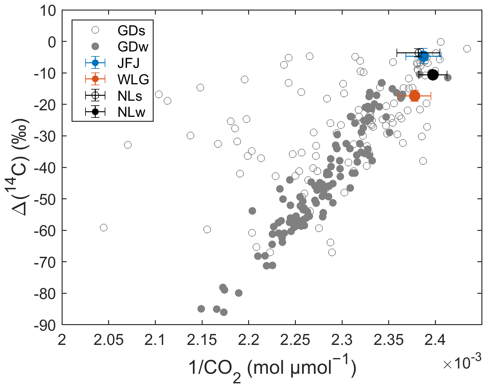
Figure 2 Keeling plot of CO₂ and Δ(¹⁴C) measurements from Guangdong Province in summer (GDs) and winter (GDw), and background stations including JFJ (Jungfraujoch) (Emmenegger et al., 2024a, b), WLG (Waliguan) (Liu et al., 2024; Lan et al., 2024), and NL (Nanling, this study) in 2022. For the JFJ background site, the complete 2022 dataset was used to calculate a true annual mean. For the WLG background site, CO₂ concentrations were obtained from the World Data Centre for Greenhouse Gases (WDCGG, https://gaw.kishou.go.jp/, last access: 21 April 2024), while Δ(¹⁴C) observations were obtained from Liu et al. (2024). For the NL background site, CO₂ and Δ(¹⁴C) observations were obtained from two campaigns in August and December 2022, representing typical summer and winter conditions.

3.2 CO₂, Δ(¹⁴C), C_xs and C_ff concentrations

CO₂ concentrations in Guangzhou, Shenzhen, Zhanjiang, and Shaoguan were (438.8±12.3), (435.0±12.7), (444.2±17.2), and $(\mathrm{431.6}\pm \mathrm{10.5})\mathrm{\mu }\mathrm{mol}{\mathrm{mol}}^{-\mathrm{1}}$ (multisite mean and one-sigma standard deviation), respectively; the corresponding Δ(¹⁴C) values were $(-\mathrm{40.7}\pm \mathrm{13.4})\mathrm{‰}$, $(-\mathrm{37.2}\pm \mathrm{24.1})\mathrm{‰}$, $(-\mathrm{28.8}\pm \mathrm{13.8})\mathrm{‰}$, and $(-\mathrm{25.0}\pm \mathrm{14.9})\mathrm{‰}$, respectively. Relative to the background, CO₂ concentrations in the four cities were enhanced by (20.3±12.5), (16.5±13.5), (25.8±16.7), and $(\mathrm{13.1}\pm \mathrm{10.1})\mathrm{\mu }\mathrm{mol}{\mathrm{mol}}^{-\mathrm{1}}$ (C_xs), respectively; the mean Δ(¹⁴C) was depleted by $(-\mathrm{33.6}\pm \mathrm{11.3})\mathrm{‰}$, $(-\mathrm{29.9}\pm \mathrm{22.3})\mathrm{‰}$, $(-\mathrm{21.5}\pm \mathrm{11.7})\mathrm{‰}$, and $(-\mathrm{17.8}\pm \mathrm{15.7})\mathrm{‰}$ (ΔΔ(¹⁴C)), respectively, reflecting the marked influence of ¹⁴C-free CO₂ emissions from fossil fuel combustion. The fossil fuel and biogenic fractions of C_xs, C_ff and C_bio, were determined using a two end-member mixing analysis. The C_ff fractions were (79±5) %, (73±6) %, (59±4) %, and (53±13) % during winter in Guangzhou, Shenzhen, Zhanjiang, and Shaoguan, respectively. In comparison with other cities worldwide (Table E1 and Fig. E1), we observed higher C_ff fractions (>70 %) in some megacities and supercities compared with large and medium-sized cities. Noting that the $C_{\mathrm{ff}}/C_{\text{xs}}$ ratio is critically sensitive to background selection. Regional backgrounds (as implemented here) introduce C_bio contributions from surrounding rural/agricultural sources to C_xs, whereas local urban backgrounds effectively isolate urban emissions by filtering out these external biogenic signals, thereby increasing the apparent C_ff fraction compared to regional background approaches. The consistent adoption of regional background methodologies across all studies in Table E1 ensures the comparative validity of the results, as they share a common framework for accounting for C_bio influences from peripheral non-urban sources. The derived annual C_ff averages are (15.3±5.2), (13.7±10.2), (10.0±5.2), and $(\mathrm{8.2}\pm \mathrm{7.0})\mathrm{\mu }\mathrm{mol}{\mathrm{mol}}^{-\mathrm{1}}$ in Guangzhou, Shenzhen, Zhanjiang, and Shaoguan, respectively, based on the mass balance equations of CO₂ and Δ(¹⁴C). These C_ff concentrations were low to moderate compared with those in other cities globally (Table E2 and Fig. E1), despite the high emissions in Guangzhou and Shenzhen from inventories (Fig. 1).

3.3 Spatial distribution and seasonal variations

The spatial differences observed in C_ff primarily reflect the combined influence of emission intensity and atmospheric transport rather than direct emission magnitudes. We first identified potential source regions that are likely to contribute to the observed C_ff variability by analyzing its spatial distribution and seasonal variations. Higher C_ff levels were typically observed at densely populated downtown sites (GZ6 and GZ5; SG3 and SG2) in Guangzhou during summer (GZs) and Shaoguan during winter (SGw), forming an “urban C_ff dome” (Fig. 1cj). This was further supported by a positive correlation between the C_ff measurements and the corresponding 1 km×1 km gridded ODIAC (Oda and Maksyutov, 2011; Oda and Maksyutov, 2024) inventory emissions in GZs (r=0.53, p=0.1), and a significant positive correlation in SGw (r=0.91, p=0.03). These correlations are used here as qualitative support and should be interpreted cautiously given uncertainties in the emission inventory (e.g., missing or spatially misallocated sources). The “urban C_ff dome” indicates that C_ff is mainly derived from the localized fossil fuel combustion, which is likely to be influenced by the urban topography. That is, downtown Guangzhou and downtown Shaoguan are surrounded by mountains to the east, north, and west. In contrast, we found that higher C_ff from western industrial areas and airport (SZ2) in Shenzhen during summer (SZs), and from port areas (ZJ5 > ZJ2; ZJ2 > ZJ3 > ZJ4) in Zhanjiang during winter (ZJw) and summer (ZJs, by atmospheric transport) (Fig. 1e, h and g).

Atmospheric transmission of C_ff from potential source regions was observed at large spatial scales combined with air mass back trajectories by the Hybrid Single-Particle Lagrangian Integrated Trajectory (HYSPLIT) model (Stein et al., 2015) and emission footprints by the FLEXPART dispersion model (Pisso et al., 2019). Shaoguan exhibited higher C_ff concentrations in summer ($(\mathrm{10.7}\pm \mathrm{8.3})\mathrm{\mu }\mathrm{mol}{\mathrm{mol}}^{-\mathrm{1}}$) than in winter ($(\mathrm{5.8}\pm \mathrm{4.4})\mathrm{\mu }\mathrm{mol}{\mathrm{mol}}^{-\mathrm{1}}$). Trajectory and footprint analyses suggest that summer observations at Shaoguan were frequently influenced by air masses arriving from the Pearl River Delta (PRD) urban agglomeration (HYSPLIT, Fig. F1a; FLEXPART, Fig. 3g), consistent with a larger upwind contribution under prevailing transport conditions. We note that the inference of “local versus non-local” contributions is conditional on the completeness and spatial allocation of the emission inventories. In contrast, we found higher C_ff concentrations in winter compared with those in summer in Guangzhou ($(\mathrm{17.7}\pm \mathrm{3.5})>(\mathrm{12.9}\pm \mathrm{5.6})\mathrm{\mu }\mathrm{mol}{\mathrm{mol}}^{-\mathrm{1}}$), Shenzhen ($(\mathrm{18.0}\pm \mathrm{9.9})>(\mathrm{9.2}\pm \mathrm{8.5})\mathrm{\mu }\mathrm{mol}{\mathrm{mol}}^{-\mathrm{1}}$), and Zhanjiang ($(\mathrm{12.1}\pm \mathrm{5.1})>(\mathrm{7.6}\pm \mathrm{4.3})\mathrm{\mu }\mathrm{mol}{\mathrm{mol}}^{-\mathrm{1}}$), consistent with the values in 14 other Chinese cities (Zhou et al., 2020). The higher winter concentrations likely reflect a combination of (i) reduced ventilation (e.g., a shallow planetary boundary layer), and (ii) higher wintertime emissions suggested by ODIAC/MEIC (winter emissions 8 %, 10 %, and 11 % [ODIAC] and 17 %, 22 %, and 14 % [MEIC] higher than summer for Guangzhou, Shenzhen, and Zhanjiang, respectively (Oda and Maksyutov, 2024; MEIC, 2023)), noting the associated inventory uncertainties. Within Guangzhou (GZw) and Shenzhen (SZw), wintertime spatial gradients show higher C_ff concentrations at downwind sites (GZ2, GZ6, and GZ10; SZ3 and SZ4) than at upwind sites (GZ1 and GZ3; SZ8 and SZ9), suggesting an important role of transport/accumulation in shaping the observed enhancements. The air mass back trajectories (HYSPLIT, Fig. F1b) and emission footprints (FLEXPART, Fig. 3b and d) showed that the major source region was traced to the Yangtze River Delta (YRD) urban agglomeration in East China, and a portion from North China via long-range transport (Fig. F2e and f). The major source region from the YRD was also reported in a study of CFC-11 in Shenzhen (Chen et al., 2024).

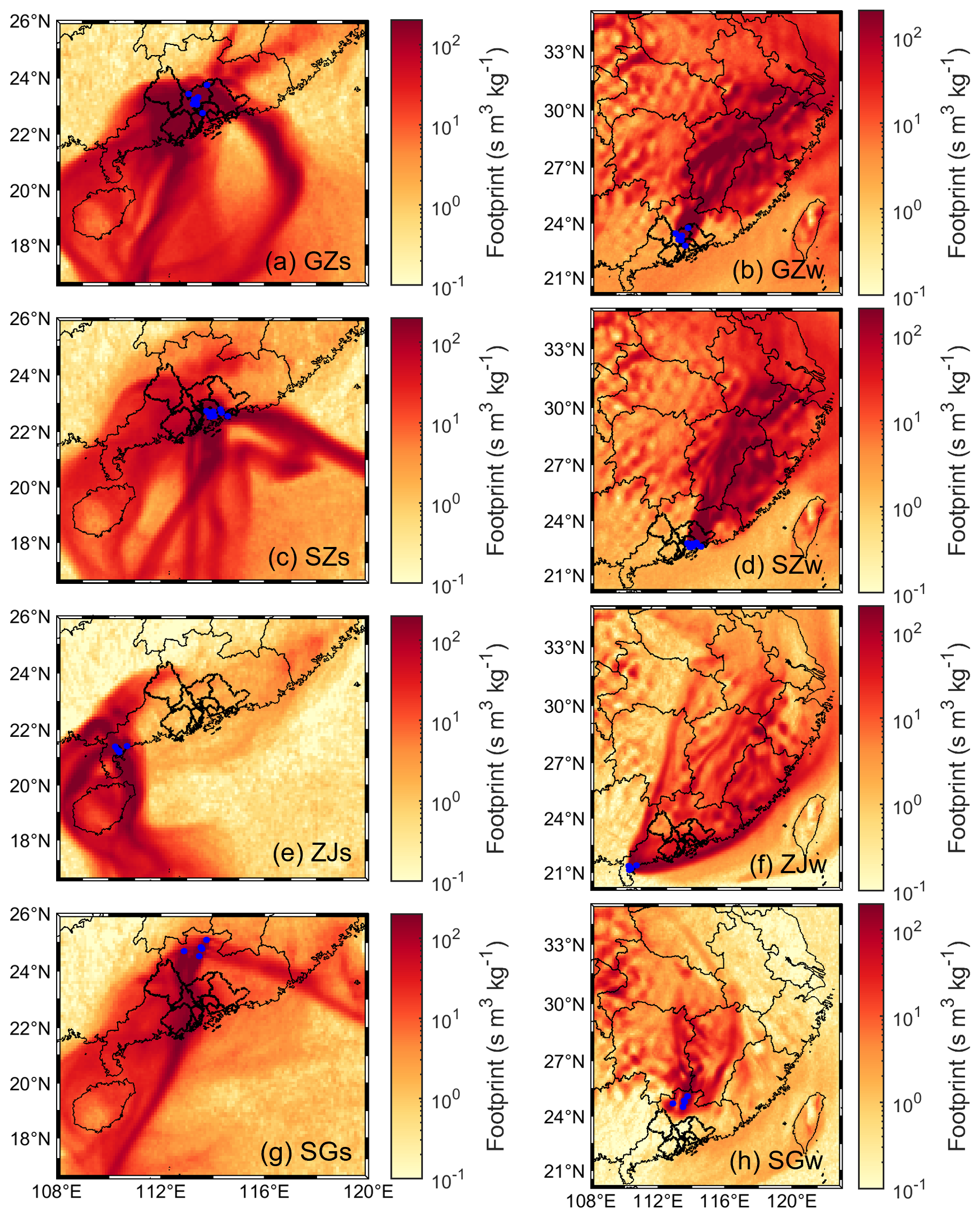
Figure 3 FLEXPART footprints simulating C_ff emissions in summer (s) and winter (w) for (a, b, GZ) Guangzhou, (c, d, SZ) Shenzhen, (e, f, ZJ) Zhanjiang, and (g, h, SG) Shaoguan at heights from 0–100 m a.s.l. over a period of 30 d. Blue points represent the locations of sampling sites. Black lines indicate the boundaries of continents (left), Chinese provinces (left, bold), and the nine cities of the PRD (right, bold) taken from Natural Earth (https://www.naturalearthdata.com/, last access: 9 March 2024).

3.4 Historical variations

3.4.1 Meteorological typicality of sampling months

As shown in Fig. G1, all five meteorological variables (10 m eastward wind, U10; 10 m northward wind, V10; 2 m air temperature, T2M; surface pressure, SP; and planetary boundary-layer height, PBLH) at all Guangzhou sites exhibit $\left|z\right|\le \mathrm{1}$, indicating that both August and December 2022 were meteorologically typical relative to the same-year seasonal background and the 2010–2022 climatological baselines. At GZ7, December 2010 also shows $\left|z\right|\le \mathrm{1}$ relative to both the DJF 2010 seasonal mean and the 2010–2022 DJF climatology, indicating that the 2010 winter sampling month was likewise meteorologically typical (Fig. G1e–f). August 2022 featured slightly weaker easterly winds and near-climatological boundary-layer heights, while December 2022 was characterized by prevailing northerly flow and typical boundary-layer ventilation. Similarly, all five variables for December 2010 at GZ7 remained within ±1σ of both the DJF 2010 mean and the 2010–2022 DJF climatology, confirming that the 2010 winter sampling month was not associated with unusual circulation or mixing conditions.

Complementary ERA5 wind-rose analyses (Fig. G2) and 72 h HYSPLIT back-trajectory simulations (Fig. F1) confirm that both months followed the canonical East Asian monsoon regimes – maritime inflow during summer and continental outflow during winter. Using GZ7 as an illustrative example representative of central Guangzhou, the ERA5 wind roses show dominant east–east-southeasterly (90–135°) winds in August 2022, typically 3–8 m s⁻¹. In comparison, JJA 2022 and the 2010–2021 JJA climatology peak in the south–south-westerly sector (157.5–225°), representing a within-sector rotation (90–225°) rather than a regime change. ERA5 anomalies of U10, V10, and PBLH remain below 1σ, confirming transport typicality. HYSPLIT trajectories indicate that August 2022 air masses primarily originated over the South China Sea, consistent with summer maritime inflow. For December 2022, the ERA5 wind roses display a clear north–north-easterly (0–45°) dominance with 3–8 m s⁻¹ speeds. The DJF 2022 composite and the 2010–2021 DJF climatology show nearly identical northerly continental patterns, typical of the East Asian winter monsoon. HYSPLIT back trajectories confirm that the air parcels predominantly arrived from northern continental China under prevailing northerlies. Similarly, the ERA5 wind roses for December 2010 and DJF 2010 at GZ7 (Fig. G2g–h) show dominant northerly to north-easterly flow, closely matching the DJF climatological wind regime, indicating that the 2010 winter sampling period was also embedded in the canonical East Asian winter monsoon pattern.

To directly compare the meteorological environments of the two sampling years, we further analysed ERA5 diagnostics on flask sampling days at GZ7 (Tables G1 and G2). Both December 2010 and December 2022 were dominated by northerly to north-easterly flow, with winds in the 0–45° sector accounting for 61.7 % and 82.7 % of occurrences, respectively (Table G2). However, December 2022 exhibited stronger winds and deeper boundary layers than December 2010 (mean wind speed: 3.6 vs. 2.6 m s⁻¹; mean PBLH: 476 vs. 377 m; mean ventilation: 2024.5 vs. 1258.0 m² s⁻¹), and these differences are statistically significant (p<0.01 for both Student's t-test and Mann–Whitney U test; Table G1). These conditions would tend to dilute near-surface enhancements in 2022 relative to 2010, implying that the observed decreases in C_ff and $R_{\mathrm{CO}/{\mathrm{CO}}_{\mathrm{2}\mathrm{ff}}}$ between the two periods are, if anything, conservative with respect to emission changes.

Overall, these diagnostics suggest that the sampling windows in both 2010 and 2022 were not associated with anomalous large-scale transport. Nevertheless, variability in mixing and transport at sub-monthly scales may still contribute to uncertainty, especially given the limited number of winter flasks in 2022. Accordingly, we treat transport/mixing variability as an uncertainty in the inter-period comparison rather than assuming it to be negligible.

3.4.2 Representativeness of weekly flask samples

Each flask represents approximately 15–20 min of integrated air, and about 40 samples were collected per month across ten stations, providing broad spatial and temporal coverage. To evaluate how representative these discrete samples are for the respective seasons, we compared ERA5 diagnostics (PBLH, wind speed, and wind direction) during sampling days with the corresponding monthly means. The results show that meteorological conditions during sampling closely matched monthly climatological averages, confirming that no unusual stagnation or transport anomalies occurred on the sampling days. For the December 2010 flask sampling at GZ7, ERA5 diagnostics and wind roses (Figs. G1e, f and G2g, h) likewise show that sampling-day conditions were consistent with the DJF 2010 seasonal mean and the 2010–2022 DJF climatology, indicating that these earlier samples were also collected under typical winter transport regimes.

ERA5 wind roses (Fig. G2) and HYSPLIT 72 h back-trajectories (Fig. F1) further confirm that the flask collection periods coincided with the prevailing summer (90–225°) and winter (0–45°) monsoon sectors. Hence, the samples captured the dominant seasonal transport regimes rather than isolated short-term events. We therefore consider the weekly flask observations to be broadly representative of their seasonal backgrounds in terms of large-scale transport, while noting that the discrete nature of flask sampling (and the small winter 2022 sample size) limits the ability to fully average out synoptic-scale variability.

3.4.3 Historical variation of C_ff concentrations

To ensure comparability, all available historical datasets (Table H1) were harmonized to identical sites, seasons, and local-time windows, and recalculated using unified background references (Table H2 and Fig. 4a). This harmonization reduces methodological differences (e.g., background choice and sampling-window differences) and facilitates an inter-period comparison of C_ff mole fractions, while transport and mixing variability remains a source of uncertainty. We emphasize that the following comparison addresses observed near-surface C_ff concentrations. Without an atmospheric transport model and inverse modelling, we cannot quantitatively attribute the observed inter-period concentration differences to emission changes.

For Guangzhou, a site-specific long-term comparison was conducted at the GZ7 urban station, which was also used by Ding et al. (2013). In their study, C_ff was derived from flask observations collected around 20:00 LT (post-rush-hour) using a Δ(¹⁴C) background based on corn-leaf samples from Qinghai, Gansu, and Tibet. Such a background likely represents a different air-mass domain from Guangzhou. In contrast, the present study used atmospheric Δ(¹⁴C) observations from the NL regional background site, which directly samples the same regional air masses influencing Guangzhou. To harmonize the background reference used in the C_ff calculation between studies, the winter 2010 C_ff values from Ding et al. (2013) and the winter 2022 values from this work were recalculated using the NL tree-ring Δ(¹⁴C) record (Li et al., 2025b) as a common reference baseline. The NL tree-ring Δ(¹⁴C) represents a growing-season (March–October) integrated proxy and the 2022 value is linearly extrapolated from the 2011–2020 record; it is therefore not intended to represent wintertime background variability and is used here only to provide an internally consistent baseline for inter-study comparison. This adjustment changes C_ff from 45.6±5.3 to $\mathrm{44.2}\pm \mathrm{5.3}\mathrm{\mu }\mathrm{mol}{\mathrm{mol}}^{-\mathrm{1}}$ for 2010, and from 16.8±3.4 to $\mathrm{12.5}\pm \mathrm{3.4}\mathrm{\mu }\mathrm{mol}{\mathrm{mol}}^{-\mathrm{1}}$ for 2022.

Because sampling times differ (20:00 vs. 14:00 LT), we quantified the expected diurnal C_ff contrast using continuous CO observations near GZ7. ΔCO increased from 168 ppb at 14:00 to 221 ppb at 20:00, corresponding to a 21 % C_ff nighttime enhancement (Scheme 1, Appendix H1). A supplementary analysis using the winter 2023–2024 dataset gave a 35 % enhancement (Scheme 2, Appendix H1). These findings suggest that the evening C_ff level is typically 21 %–35 % higher than the well-mixed afternoon value due to weaker nocturnal boundary-layer mixing, although a diurnal cycle in emissions may also contribute to this difference. Applying this correction, the 2010 nighttime C_ff ($\mathrm{44.2}\pm \mathrm{5.3}\mathrm{\mu }\mathrm{mol}{\mathrm{mol}}^{-\mathrm{1}}$) corresponds to an afternoon-equivalent concentration between 28.7±3.5 and $\mathrm{34.9}\pm \mathrm{4.2}\mathrm{\mu }\mathrm{mol}{\mathrm{mol}}^{-\mathrm{1}}$, which remains substantially higher than the 2022 value of $\mathrm{12.5}\pm \mathrm{3.4}\mathrm{\mu }\mathrm{mol}{\mathrm{mol}}^{-\mathrm{1}}$.

In addition to harmonizing background Δ(¹⁴C) and sampling times, we explicitly evaluated the impact of changes in boundary-layer mixing between 2010 and 2022 (Sect. 3.4.1 and Table G1). To assess how much of the inter-period difference could plausibly be explained by changes in boundary-layer mixing, we provide a first-order estimate of the sensitivity of near-surface C_ff to PBLH variations. Under a well-mixed boundary-layer “box” approximation, the surface enhancement of predominantly surface-emitted tracers scales approximately as $C_{\mathrm{ff}}\propto \mathrm{1}/\text{PBLH}$, implying $\mathrm{\Delta }{C}_{\mathrm{ff}}/C_{\mathrm{ff}}\approx -\mathrm{\Delta }\text{PBLH}/\text{PBLH}$. Using ERA5 PBLH at the actual flask sampling hours (Fig. G1), the standardized anomaly of PBLH in Dec 2022 at Guangzhou sites is z≈0.17, corresponding to a relative PBLH increase of 11 % (based on the local winter mean and standard deviation used to define z). If emissions and other factors were unchanged, this would translate into an expected dilution of C_ff by 11 % (i.e., 1–3 µmol mol⁻¹ for typical wintertime C_ff levels). This indicates that the modestly higher PBLH in December 2022 would tend to reduce the observed C_ff, but its magnitude is smaller than the observed inter-period difference (16.2–22.4 µmol mol⁻¹).

Taken together, after harmonizing the Δ(¹⁴C) background and accounting for sampling-time differences, the observations indicate an indicative inter-period decrease in wintertime C_ff in Guangzhou between 2010 and 2022. Using the CO-based diurnal scaling (21 %–35 % nighttime enhancement), the 2010 value corresponds to an afternoon-equivalent C_ff of 28.7–34.9 µmol mol⁻¹, compared to $\mathrm{12.5}\pm \mathrm{3.4}\mathrm{\mu }\mathrm{mol}{\mathrm{mol}}^{-\mathrm{1}}$ in 2022 (i.e., 56 %–64 % lower; the range reflects uncertainty in the diurnal scaling). This percentage refers to the observed concentration change and may include a modest contribution from differences in boundary-layer mixing; our first-order PBLH-based scaling suggests that the December 2022 mixing anomaly would affect C_ff at the ∼10 % level (1–3 µmol mol⁻¹). Given the limited number of winter flasks in 2022, we performed a leave-one-out sensitivity test (Appendix H), which shows that the inferred 2010–2022 decrease remains negative for all subsets, although the magnitude varies. Accordingly, we interpret the Guangzhou 2010–2022 difference as an indicative inter-period change rather than a robustly quantified long-term trend. FLEXPART footprint analyses for 2010 and 2022 show similar source-sensitivity patterns centered on the Guangzhou urban core, supporting that GZ7 remains representative of Guangzhou's urban influence domain in both periods.

Comparable harmonized analyses were performed for other Chinese cities (Tables H1 and H2; Fig. 4a). For Beijing, all measurements originate from the urban rooftop site of the Research Center for Eco-Environmental Sciences, Chinese Academy of Sciences (RCEES). The Δ(¹⁴C) background used in Zhou et al. (2020) was based on Qixianling Mountain (QXL), whereas Wang et al. (2022b) adopted the Waliguan (WLG) background. All C_ff values were recalculated using WLG as a common reference background with the 2015 value from Niu et al. (2016). After this correction, the 2014–2016 winter C_ff value increases slightly from 27.0±0.3 to $\mathrm{27.6}\pm \mathrm{0.3}\mathrm{\mu }\mathrm{mol}{\mathrm{mol}}^{-\mathrm{1}}$, ensuring consistency across datasets. Relative to this harmonized baseline, the subsequent decline to 19.7±22.0 µmol mol⁻¹ by winter 2020 (Wang et al., 2022b) represents an approximate 29 % reduction (p<0.05). This trend is consistent with regional fossil-fuel CO₂ emission reductions and corroborated by independent Δ(¹⁴C) tree-ring records showing a peak near 2010 in Beijing (Niu et al., 2024). For Xi'an, at the Institute of Earth Environment, Chinese Academy of Sciences (IEECAS) urban site, C_ff fell by 36 % from $(\mathrm{40.1}\pm \mathrm{3.8})\mathrm{\mu }\mathrm{mol}{\mathrm{mol}}^{-\mathrm{1}}$ in 2011–2013 to $(\mathrm{25.7}\pm \mathrm{1.1})\mathrm{\mu }\mathrm{mol}{\mathrm{mol}}^{-\mathrm{1}}$ in 2014–2016 (p<0.001) (Zhou et al., 2022). Suburban sites declined by ≈12 % from $(\mathrm{23.5}\pm \mathrm{6.5})\mathrm{\mu }\mathrm{mol}{\mathrm{mol}}^{-\mathrm{1}}$ in 2016 (Wang et al., 2018) to $(\mathrm{13.1}\pm \mathrm{10.9})\mathrm{\mu }\mathrm{mol}{\mathrm{mol}}^{-\mathrm{1}}$ in 2021–2022 (Liu et al., 2024) (p<0.05). These decreases are consistent with independent Δ(¹⁴C) tree-ring records indicating emission peak near 2013 in Xi'an (Niu et al., 2024).

Overall, the harmonized, site-specific, and time-of-day-corrected comparisons demonstrate statistically significant reductions in fossil-fuel CO₂ across China's major urban centers. For Guangzhou particularly, the combined evidence – consistent background domain, typical meteorology, verified sampling representativeness, and quantified diurnal correction – provides strong support that the observed C_ff decline reflects genuine decarbonization rather than artifacts of sampling or transport variability. Furthermore, this observed decline in C_ff is consistent with reported emission reductions in major source regions of South and East China (e.g., Hebei, Shandong, Zhejiang, and Guangdong; Fig. F2) according to the MEIC inventory (Shi et al., 2022), supporting the interpretation of a widespread decarbonization trend.

Similar reductions were found in C_ff emissions from 2012–2020 according to the MEIC inventory (Shi et al., 2022), such as Guangzhou (by 16 % from 2011), Shenzhen (by 3 %), Zhanjiang (by 0.1 %), Beijing (by 16 %), and Xi'an (by 9 %) (Fig. 4b), particularly in the industrial and power sectors (Li et al., 2017). We also found such declines in the MIXv2 Asian emission inventory (MIXv2, excluding Shenzhen and Shaoguan) (Li et al., 2024) and another carbon inventory for most Chinese cities (Zhang et al., 2024), but not in the ODIAC (Oda and Maksyutov, 2024) and the Emissions Database for Global Atmospheric Research (EDGAR) (Crippa et al., 2023). In fact, the mitigation of C_ff emissions in China's MEIC inventory was primarily driven by heterogeneous trends across cities: 38 % exhibited sustained emission reductions, 29 % showed an initial decline followed by a rebound, while 33 % maintained increasing trajectories. Notably, cities achieving sustained reductions were disproportionately concentrated in larger cities, comprising 86 % of megacities, 43 % of supercities, and 43 % of Type I large cities (populations of 3–5 million). In contrast, smaller cities showed lower mitigation prevalence, with only 34 % of Type II large cities (1–3 million) and 38 % of medium/ small cities attaining emission decreases.

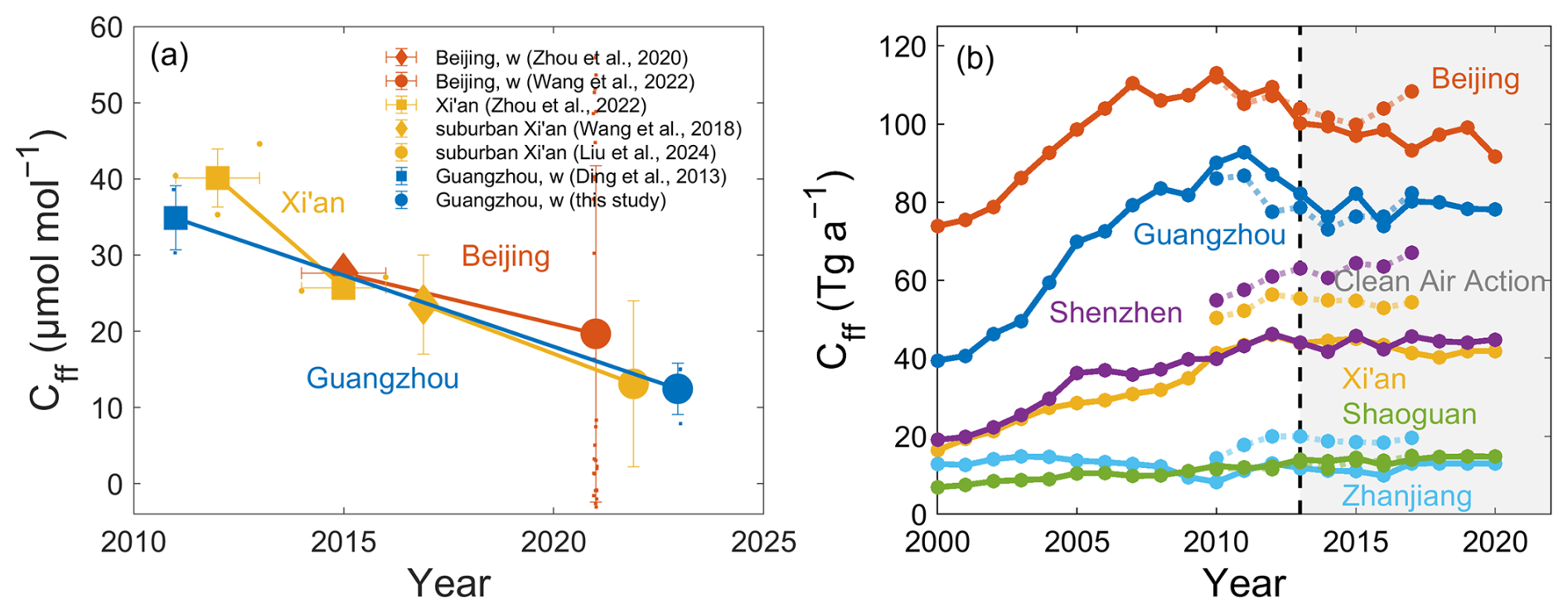
Figure 4 (a) Harmonized comparison of C_ff mole fractions at the same sites and seasons, after applying consistent sampling time and background assumptions. C_ff concentrations are compiled from atmospheric measurements (Wang et al., 2022b; Zhou et al., 2022, 2020; Ding et al., 2013; Wang et al., 2018) in Beijing, Xi'an, and Guangzhou. Large symbols indicate annual means, multiyear averages, or winter means (w) of the harmonized C_ff values listed in Table H2; small symbols represent the corresponding individual measurements. C_ff is calculated as enhancements over the regional background (Nanling for Guangzhou; Waliguan for Beijing and Xi'an). For Guangzhou, the inter-study harmonization in Table H2 uses a common NL tree-ring Δ(¹⁴C) reference baseline (growing-season integrated; extrapolated to 2022 from the 2011–2020 record; Li et al., 2025b) to harmonize background definitions across studies (used for harmonization only, not as a winter background). The y axis error bars indicate uncertainty, and the x axis error bars represent the observed period. (b) C_ff emissions from the MEIC (solid lines) (Li et al., 2017; Meic, 2023; Zheng et al., 2018) and MIXv2 (dotted lines) (Li et al., 2024) inventories in Beijing, Xi'an, Guangzhou, Shenzhen, Zhanjiang, and Shaoguan since 2010. The vertical dashed line indicates the year 2013 when China's Clean Air Action Plan was implemented.

3.5 Driver factors

3.5.1 Coal-to-gas transition

We determined the coal, oil, and natural gas fractions of C_ff using the Keeling plot of δ(¹³C) and CO₂ (i.e., scatter plot between δ(¹³C) and inverse of CO₂ mole fractions) and the Bayesian mixing model (MixSIAR) (Stock et al., 2018) during winter 2022. The fractions in winter were (49±25) %, (29±22) %, and (22±19) %, respectively, for Guangzhou, (47±25) %, (29±21) %, and (24±20) % for Shenzhen, (43±24) %, (29±21) %, and (28±21) % for Zhanjiang, and (39±24) %, (34±23) %, and (27±21) % for Shaoguan (Table I1). Coal combustion was the largest contributor to C_ff emissions, followed in descending order by oil combustion and natural gas combustion. Compared with other cities around the world (Table I1), we found natural gas was the primary fuel type consumed in Paris (70 %) (Lopez et al., 2013) and Beijing (55±9 %) (Wang et al., 2022b), whereas oil was the main fuel type consumed in Los Angeles (>50 %) (Djuricin et al., 2010; Newman et al., 2016). Coal remains the primary fossil fuel used in Xi'an ((72.6±10.4) % in 2014 and (54±4) % in 2019) (Wang et al., 2022b; Zhou et al., 2014), Guangzhou (49 % in 2022), and Shenzhen (47 % in 2022). Notably, cities with high C_ff emissions consume all three types of fossil fuels, with the dominant fuel type varying by city. Coal remains the primary fossil fuel used in many Chinese cities.

The reduction in C_ff concentrations can be attributed to changes in energy systems as a result of China's clean air measures (Shi et al., 2022). A major contribution has been the reduction in coal usage and the shift to low-carbon energy sources such as natural gas. During 2013–2022, the share of coal in the energy mix decreased by 4.9 % in China and by 7.1 % in Guangdong Province, whereas the share of natural gas increased by 3.0 % in China and by 7.2 % in Guangdong Province, according to the MEIC inventory (Li et al., 2017; Zheng et al., 2018; Meic, 2023; Xu et al., 2024). By applying the coal, oil, and natural gas fractions of C_ff derived from our measurements, it's likely that coal usage in Guangdong Province since 2013 have decreased ≥21 %, and natural gas usage have increased by ≥16 % (Fig. 5a). Similarly, in Guangzhou city, it's likely that coal usage since 2011 has decreased by 23 % instead of by 8.8 % (Fig. 5b), and natural gas usage has increased by 17 % instead of by 7.9 %, assuming that the fuel type fractions of C_ff in Guangzhou city were the same as those in Guangdong Province in the inventory.

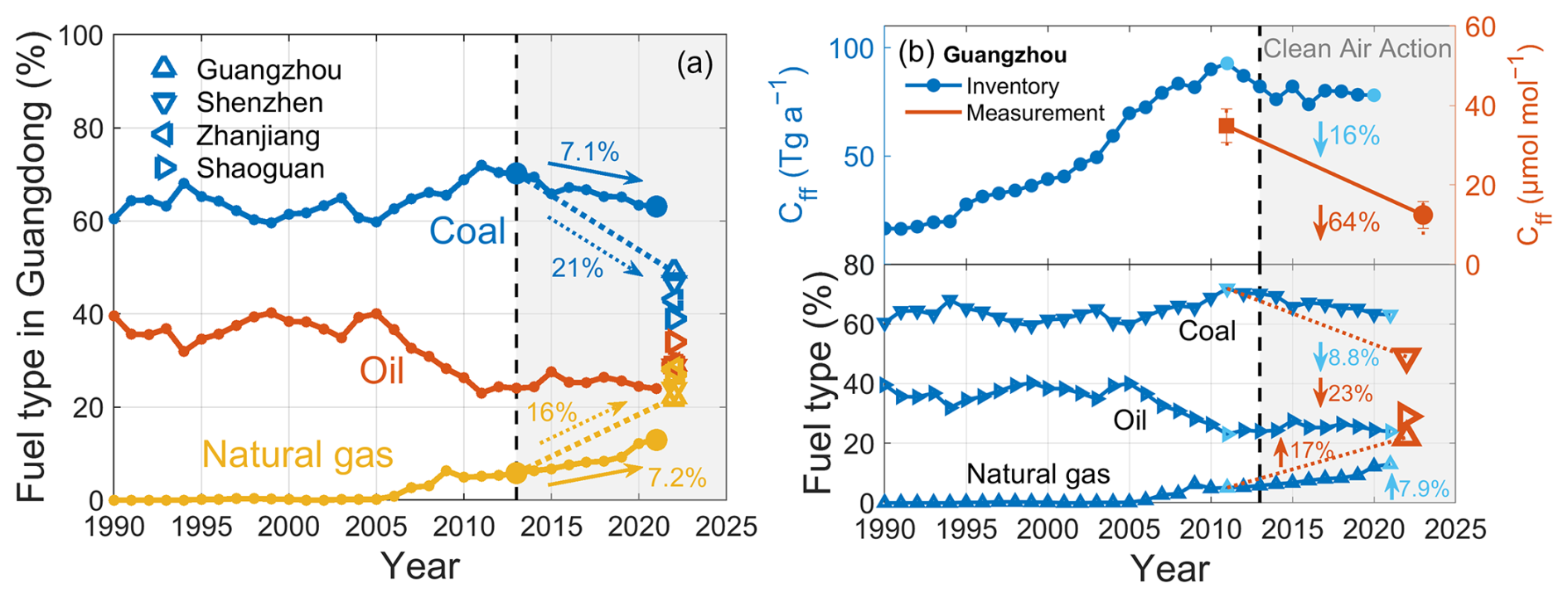
Figure 5 (a) Coal, oil, and natural gas fractions of C_ff in Guangdong Province from the MEIC inventory from 1990–2021 (points), and in the cities of Guangzhou, Shenzhen, Zhanjiang, and Shaoguan from measurements in this study in 2022 (triangles). (b) (Top) Comparison of reductions in C_ff inventory emissions (blue) and harmonized measured C_ff concentrations in Guangzhou (red; harmonized by applying consistent sampling-time and background assumptions) resulting from (Bottom) reduced coal usage and increased natural gas usage in Guangzhou. The vertical dashed line indicates the year 2013 when China's Clean Air Action Plan was implemented.

3.5.2 Combustion efficiency improvement

We calculated $R_{\mathrm{CO}/{\mathrm{CO}}_{\mathrm{2}\mathrm{ff}}}$ ratios at each measurement site and found higher ratios in summer than winter (Fig. J1). However, we focused only on observations in winter for four reasons. First, summer CO shows greater instability as its atmospheric lifetime depends on OH radical production, which is enhanced through photochemical reactions (e.g., CH₄ oxidation) under intense solar radiation, making CO a less reliable fossil fuel tracer (Rosendahl, 2022). Second, winter exhibits stronger ΔCO-C_ff correlations (r>0.6, p<0.01; Fig. J2) with better regional representativeness due to extended CO atmospheric lifetime from slower CO oxidation rates. Third, the winter ΔCO-C_ff relationship better captures anthropogenic emission characteristics compared to other seasons. Fourth, weaker vertical mixing in winter accentuates local emission impacts (Wang et al., 2010). In addition, the lower C_ff signals observed in summer lead to higher uncertainty in the regression slope and thus greater uncertainty in the $R_{\mathrm{CO}/{\mathrm{CO}}_{\mathrm{2}\mathrm{ff}}}$ ratios, as also noted in Maier et al. (2024), which can be seen in the larger error bars of the summer data in Fig. J2.

We then estimated winter 2022 $R_{\mathrm{CO}/{\mathrm{CO}}_{\mathrm{2}\mathrm{ff}}}$ ratios across Chinese cities using ΔCO-C_ff regression slopes (Fig. J2), with spatial variations primarily attributed to differences in fuel composition and combustion efficiency (Graven et al., 2009). CO is generated through incomplete combustion of both fossil fuels and biomass. These spatial patterns are consistent with combustion characteristics showing biomass burning produces higher CO emissions per unit energy than fossil fuel combustion (Akagi et al., 2011). As shown in Fig. J1, suburban/rural sites (GZ1, SZ9, ZJ1, SG1) exhibited significantly higher ratios than urban sites (GZ5, SZ7, ZJ4, SG3): GZ1 > GZ5 ((30.4±10.0) > (19.8±4.6) nmol µmol⁻¹), SZ9 > SZ7 ((41.3±23.0) > (14.8±2.4) nmol µmol⁻¹), ZJ1 > ZJ4 ((41.2±3.6) > (11.9±6.4) nmol µmol⁻¹), and SG1 > SG3 ((26.7±2.9) > (15.1±3.6) nmol µmol⁻¹). This pattern is in agreement with previous studies attributing elevated ratios in non-urban areas to biomass burning contributions (Rosendahl, 2022). In contrast, megacities showed 35 %–40 % lower ratios (Guangzhou: $\mathrm{13.3}\pm \mathrm{3.1}\mathrm{nmol}\mathrm{\mu }{\mathrm{mol}}^{-\mathrm{1}}$, Shenzhen: $\mathrm{13.5}\pm \mathrm{2.4}\mathrm{nmol}\mathrm{\mu }{\mathrm{mol}}^{-\mathrm{1}}$) compared to smaller cities (Zhanjiang: $\mathrm{22.6}\pm \mathrm{5.0}\mathrm{nmol}\mathrm{\mu }{\mathrm{mol}}^{-\mathrm{1}}$, Shaoguan: $\mathrm{21.7}\pm \mathrm{6.4}\mathrm{nmol}\mathrm{\mu }{\mathrm{mol}}^{-\mathrm{1}}$; p<0.01; Fig. J2), suggest higher fossil fuel combustion efficiency and/or lower biomass burning inputs. Guangzhou's ratios are dominated by improved fossil fuel combustion efficiency due to having the highest biomass burning emissions among the four studied cities in the EDGAR2024 inventory, while Shenzhen's ratios are attributed to both factors with nearly negligible biomass contributions corresponding to its 2017 biomass boiler phase-out policy.

We retrieved historical $R_{\mathrm{CO}/{\mathrm{CO}}_{\mathrm{2}\mathrm{ff}}}$ data from observations in China by estimation from Δ(¹⁴C) measurements and correction from $R_{\mathrm{CO}/{\mathrm{CO}}_{\mathrm{2}}}$ (increased by 20 %) (Table J1), and $I_{\mathrm{CO}/{\mathrm{CO}}_{\mathrm{2}\mathrm{ff}}}$ data from the MEIC, MIXv2, and EDGAR inventories (Fig. 6). Because the observational record consists of discrete campaigns, for the observations we assess changes using inter-period differences (rather than fitting a single 1998–2022 linear trend), and we test robustness by comparing the inferred change with the combined 1σ uncertainties (added in quadrature, using the reported vertical 1σ uncertainties for each period). Given the minor contribution of biomass burning (BB)-related CO emissions across all inventories, with $I_{\mathrm{CO}/{\mathrm{CO}}_{\mathrm{2}\mathrm{ff}}}$ ratio below 0.003 (MEIC, incorporating OBBEIC data (Song et al., 2009; Huang et al., 2012)), less than 1.0 (MIXv2), and declining from 3.8 (1990) to 1.1 (2022) in EDGAR, we assume that interannual variability in BB emissions has negligible influence on the overall emission ratios. The compiled observations (1998–2022) and inventories (1990–2022) both indicate $R_{\mathrm{CO}/{\mathrm{CO}}_{\mathrm{2}\mathrm{ff}}}$ and $I_{\mathrm{CO}/{\mathrm{CO}}_{\mathrm{2}\mathrm{ff}}}$ ratios tend to be lower in recent years than in earlier periods (Fig. 6a), consistent with improved combustion efficiency (Wang et al., 2010; Lee et al., 2020), which is another factor contributing to the reduction in C_ff concentrations. The MEIC inventory attributes this trend to spatiotemporally heterogeneous mitigation pathways: 72 % of the cities started $I_{\mathrm{CO}/{\mathrm{CO}}_{\mathrm{2}\mathrm{ff}}}$ reductions during 1990–1994, while the remaining 28 % (mainly concentrated in the western provinces) exhibited a delayed start until 1995–2004. The implementation of China's clean air policies since 2013 has systematically phased out small, inefficient combustion facilities and replaced them with centralized, high efficient, and clean energy infrastructure (Shi et al., 2022). The phase-out of coal-fired industrial boilers during 2013–2020 reduced CO₂ emissions by (1.5±0.3) Gt, accounting for 12 % of the national industrial emission reduction (Li, 2023). These technological transitions enhanced combustion efficiency by >10 %, and reduced coal-dominated energy intensity by 40 % across the sector. The MEIC inventory showed that these synergistic measures resulted in significant energy savings, with a net reduction of 0.25 gigatonnes of coal equivalent (Gtce) in 2020 and a cumulative reduction of 1.06 Gtce over the policy implementation period (Shi et al., 2022). Critically, the efficiency-driven transition decoupled energy demand from C_ff emissions, with combustion optimization directly reducing coal consumption 1 %–2 % and C_ff emissions by 1–3 Gt yr⁻¹ after 2015 (Le Quéré et al., 2016; Friedlingstein et al., 2023b).

We systematically compared observational $R_{\mathrm{CO}/{\mathrm{CO}}_{\mathrm{2}\mathrm{ff}}}$ values with inventory $I_{\mathrm{CO}/{\mathrm{CO}}_{\mathrm{2}\mathrm{ff}}}$ estimates. Our 2022 measurements of the $R_{\mathrm{CO}/{\mathrm{CO}}_{\mathrm{2}\mathrm{ff}}}$ ratios in megacities (Guangzhou and Shenzhen) were consistent with EDGAR estimates (14.9 nmol µmol⁻¹, 2022), while those in smaller cities (Zhanjiang and Shaoguan) were closer to MEIC values (19.2 nmol µmol⁻¹, 2020) (Fig. 6a) and independent field measurements near Xi'an (23±6 nmol µmol⁻¹, 2021) (Liu et al., 2024). City comparisons of observations against MEIC estimates revealed systematic deviations: Shenzhen's observed ratio fell 42 % below inventory estimates (23.4 nmol µmol⁻¹), whereas Shaoguan's exceeded projections (12.7 nmol µmol⁻¹) by 71 %; Guangzhou's and Zhanjiang's are similar to inventory estimates (14.2 and 23.8 nmol µmol⁻¹, respectively) (Fig. 6b). When a regional background site is used, however, the inferred $R_{\mathrm{CO}/{\mathrm{CO}}_{\mathrm{2}\mathrm{ff}}}$ ratios may be influenced by emissions from outside the target city, so that the observed ratios represent a mixture of urban and regional emission signatures rather than a purely city-scale signal. This background effect may therefore contribute to some of the discrepancies between $R_{\mathrm{CO}/{\mathrm{CO}}_{\mathrm{2}\mathrm{ff}}}$ and $I_{\mathrm{CO}/{\mathrm{CO}}_{\mathrm{2}\mathrm{ff}}}$.

The 24 year observational record of $R_{\mathrm{CO}/{\mathrm{CO}}_{\mathrm{2}\mathrm{ff}}}$ ratios (1998–2022) are closer to (higher than) the MEIC estimates with a difference of (22±23) % compared with the MIXv2 and EDGAR estimates, when focusing on the ratios over time and ignoring the local deviations caused by the specific cities. These findings indicate that the MEIC inventory is more accurate than the EDGAR inventory for China. For specific cities, we found that the MEIC inventory estimates were deviated less from the observed $R_{\mathrm{CO}/{\mathrm{CO}}_{\mathrm{2}\mathrm{ff}}}$ (based on Δ(¹⁴C) measurements) in recent years than the corrected $R_{\mathrm{CO}/{\mathrm{CO}}_{\mathrm{2}\mathrm{ff}}}$ (using $R_{\mathrm{CO}/{\mathrm{CO}}_{\mathrm{2}}}$) in earlier years for Beijing and Guangzhou (Fig. 6b). For example, in Beijing, the discrepancy in the ratios between observations and inventories decreased from 22 % in 2006–2007 ($R_{\mathrm{CO}/{\mathrm{CO}}_{\mathrm{2}}}$-corrected) (Wang et al., 2010) to 8.7 % in 2009–2010 (Δ(¹⁴C)-derived) (Turnbull et al., 2011), and further declined to 7.0 % by 2014 (Δ(¹⁴C)-derived) (Niu et al., 2018). Similarly, in Guangzhou, the discrepancy dropped from 84 % in 2009–2010 ($R_{\mathrm{CO}/{\mathrm{CO}}_{\mathrm{2}}}$-corrected) (Silva et al., 2013) to 34 % in 2014–2017 ($R_{\mathrm{CO}/{\mathrm{CO}}_{\mathrm{2}}}$-corrected) (Mai et al., 2021), and eventually reached 6.4 % by 2022 (Δ(¹⁴C)-derived). These results suggest that $R_{\mathrm{CO}/{\mathrm{CO}}_{\mathrm{2}}}$ corrections should be carefully interpreted, as the effect of CO₂ from non-fossil sources can significantly bias the results, even in megacities with high C_ff emissions. For example, human respiration could bias $R_{\mathrm{CO}/{\mathrm{CO}}_{\mathrm{2}}}$ low by about 9 % at a rural site near Beijing (Wang et al., 2010; Turnbull et al., 2011).

Despite the relatively good agreement of ratios between observations ($R_{\mathrm{CO}/{\mathrm{CO}}_{\mathrm{2}\mathrm{ff}}}$) and MEIC inventory ($I_{\mathrm{CO}/{\mathrm{CO}}_{\mathrm{2}\mathrm{ff}}}$) at the national scale, observational data exhibited significantly greater $R_{\mathrm{CO}/{\mathrm{CO}}_{\mathrm{2}\mathrm{ff}}}$ reduction rates than inventory estimates when examined at the city level. From observations (Fig. 6b), in Guangzhou, $R_{\mathrm{CO}/{\mathrm{CO}}_{\mathrm{2}\mathrm{ff}}}$ decreased by 36 % from 35.8 nmol µmol⁻¹ in 2009–2010 (Silva et al., 2013) to 23.8 nmol µmol⁻¹ in winter of 2014–2017 (Mai et al., 2021) and by 63 % to 13.3 nmol µmol⁻¹ in winter 2022 (partly reflecting seasonal differences, as the Silva et al. (2013) dataset included summer observations, and partly indicating reduced CO emissions relative to C_ff due to improved combustion efficiency); in Beijing, $R_{\mathrm{CO}/{\mathrm{CO}}_{\mathrm{2}\mathrm{ff}}}$ decreased by 58 % from 72.3 nmol µmol⁻¹ in 2004 (Han et al., 2009) to 30.4 nmol µmol⁻¹ in 2014 (Niu et al., 2018); in Xi'an, $R_{\mathrm{CO}/{\mathrm{CO}}_{\mathrm{2}\mathrm{ff}}}$ decreased by 50 % from $(\mathrm{46}\pm \mathrm{13})\mathrm{nmol}\mathrm{\mu }{\mathrm{mol}}^{-\mathrm{1}}$ in 2016 (Wang et al., 2018) to $(\mathrm{23}\pm \mathrm{6})\mathrm{nmol}\mathrm{\mu }{\mathrm{mol}}^{-\mathrm{1}}$ in 2021 (Liu et al., 2024). The MEIC estimates for the above three cities decreased by 36 %, 52 %, and 21 %, respectively, over the same period. Larger reductions of the ratios were found from observations than those from the MEIC inventory (i.e., 63 %>36 % for Guangzhou, 58 %>52 % for Beijing, and 50 %>21 % for Xi'an). This conclusion holds even after artificially biasing the $R_{\mathrm{CO}/{\mathrm{CO}}_{\mathrm{2}\mathrm{ff}}}$ ratio downward by about 9 % to account for human respiration in Beijing (2004) and in Guangzhou (2009–2010 and 2014–2017). These findings suggest that the MEIC inventory may insufficiently capture, or lag, the rapid improvement in combustion efficiency and energy structure transformation in China.

The 24 year decline in China's $R_{\mathrm{CO}/{\mathrm{CO}}_{\mathrm{2}\mathrm{ff}}}$ ratios (1998–2022) demonstrates both improved fossil fuel combustion efficiency and successful implementation of air pollution control policies i.e., the success of air pollution emission reduction efforts. Our observations reveal significantly greater urban $R_{\mathrm{CO}/{\mathrm{CO}}_{\mathrm{2}\mathrm{ff}}}$ reductions than those estimated by the MEIC inventory, indicating potential underestimation of CO emission reductions relative to C_ff mitigations in current inventories. This finding aligns with previous reports of inventory underestimates for real-world CO reductions. Mai et al. (2021) showed that the MEIC inventory may underestimate cumulative reductions from fleet turnover and catalytic converter upgrades, despite China's National V standards having achieved the $\le \mathrm{1}\mathrm{g}{\mathrm{km}}^{-\mathrm{1}}$ CO emission limit since 2013. Together, these results imply that the MEIC inventory might systematically underestimate the actual effectiveness of clean air policies in reducing air pollutant emissions.

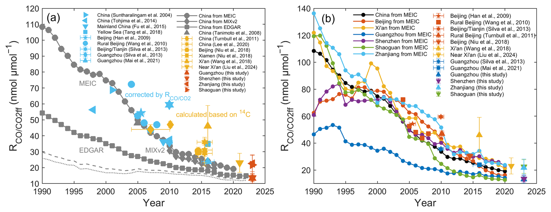
Figure 6 $R_{\mathrm{CO}/{\mathrm{CO}}_{\mathrm{2}\mathrm{ff}}}$ for (a) China and for (b) Chinses cities obtained from inventories and observations (values refer to Table H1). For (a), the gray symbols represent data from the emission inventories (Tanimoto et al., 2008), including MEIC (Meic, 2023; Xu et al., 2024; Li et al., 2019, 2017), MIXv2 (Li et al., 2024), and EDGAR2024 (EDGAR, 2024). The $I_{\mathrm{CO}/{\mathrm{CO}}_{\mathrm{2}\mathrm{ff}}}$ emission ratios derived from the three inventories are shown with distinct approaches: (1) MEIC calculated the $I_{\mathrm{CO}/{\mathrm{CO}}_{\mathrm{2}\mathrm{ff}}}$ ratio for all anthropogenic sectors (represented by solid line with point symbols); (2) MIXv2 computed two variants: combining anthropogenic sectors with open biomass burning (solid line with diamond symbols) and anthropogenic-only emissions (dash-dotted line); while (3) EDGAR2024 provided three ratios: fossil + biogenic CO (solid line with square symbols), fossil + biomass burning CO (dashed line), and fossil-only CO (dotted line), all relative to C_ff emissions. The light blue symbols represent $R_{\mathrm{CO}/{\mathrm{CO}}_{\mathrm{2}\mathrm{ff}}}$ corrected by $R_{\mathrm{CO}/{\mathrm{CO}}_{\mathrm{2}}}$ from observational studies (Wang et al., 2010; Tohjima et al., 2014; Suntharalingam et al., 2004; Tang et al., 2018; Han et al., 2009; Fu et al., 2015), assuming that 20 % of the CO₂ enhancement was from sources other than C_ff. The orange symbols represent $R_{\mathrm{CO}/{\mathrm{CO}}_{\mathrm{2}\mathrm{ff}}}$ calculated based on atmospheric ¹⁴CO₂ measurements from previous studies (Turnbull et al., 2011; Niu et al., 2018; Lee et al., 2020; Wang et al., 2018; Liu et al., 2024). The red symbols depict the values observed in this study. For (b), the Chinese cities include Beijing, Xi'an, Guangzhou, Shenzhen, Zhanjiang, and Shaoguan from the MEIC inventory (filled circles) and observations from previous studies (Wang et al., 2018, 2010; Liu et al., 2024; Silva et al., 2013; Niu et al., 2018; Mai et al., 2021; Han et al., 2009; Turnbull et al., 2011) and this study since 1990. The up and down triangles represent $R_{\mathrm{CO}/{\mathrm{CO}}_{\mathrm{2}\mathrm{ff}}}$ estimated based on atmospheric Δ(¹⁴CO₂) measurements. Other symbols represent the $R_{\mathrm{CO}/{\mathrm{CO}}_{\mathrm{2}\mathrm{ff}}}$ corrected by $R_{\mathrm{CO}/{\mathrm{CO}}_{\mathrm{2}}}$ from observational studies, assuming that 20 % of the CO₂ enhancement is from sources other than C_ff. For observation-based $R_{\mathrm{CO}/{\mathrm{CO}}_{\mathrm{2}\mathrm{ff}}}$, vertical error bars denote the uncertainty of the fitted ΔCO-C_ff regression slope. Horizontal error bars indicate the time span of each observation period, and the symbol is plotted at the median time.

3.6 Implication

Since 2013, China has implemented a series of measures with the explicit aim of improving air quality. While the initial goal of China's clean air targets was to address air pollution, they also served as a powerful catalyst for the simultaneous transformation of energy systems and the mitigation of C_ff emissions. As a result, we have observed C_ff concentration and emission reductions in some Chinese megacities and supercities, such as Guangzhou, Beijing, and Xi'an. The achievement of peak emissions in Beijing (2010) and Xi'an (2013) (Niu et al., 2024) marks a pivotal transition for China, signaling that cities across the nation, from megacities to small cities, are gradually reaching their emission peaks. This milestone has profound implications for both China's sustainable development and global climate governance, as China has dominated the global trend since 2010 (Friedlingstein et al., 2023a).

Despite China's remarkable success in reducing C_ff emissions, continued efforts are needed to optimize the nation's energy system and economic structure in order to facilitate future green growth. It is imperative that common solutions to climate change and air pollution are formulated and implemented with urgency, as China has set a goal for all cities to meet current air quality standards by 2035 and has pledged to achieve carbon peak by 2030 and carbon neutrality by 2060. One available solution is to control the common key sources and dominant source regions of air pollution and CO₂ emissions (Wu et al., 2022; Zheng et al., 2024). In future policymaking, it is essential to adopt a co-beneficiary strategy that co-ordinates clean air measures and addresses climate change measures. This strategy, together with the associated assessment approach, will be an essential part of achieving sustainable development.

4 Conclusions and outlook

This study advances the understanding of urban C_ff concentration changes in China through three key contributions. First, we provide a comprehensive error analysis framework for C_ff estimation, including contributions from air–sea exchange, nuclear facilities, and particularly biomass burning. Second, we identify inter-period decreases in observed C_ff concentrations in cities and their source regions, which are consistent with coal-to-gas transitions (evidenced by stable isotope analysis) and combustion efficiency improvements (supported by declining $R_{\mathrm{CO}/{\mathrm{CO}}_{\mathrm{2}\mathrm{ff}}}$ ratios), where megacities and supercities lead this decline. Finally, through systematic analysis of long-term $R_{\mathrm{CO}/{\mathrm{CO}}_{\mathrm{2}\mathrm{ff}}}$ trends, we reveal current emission inventories may underestimate combustion efficiency gains and CO emission reductions relative to C_ff mitigations. These findings provide critical support for refining emission accounting systems and developing evidence-based climate policies. The integrated approach offers new insights into urban emission dynamics and mitigation effectiveness.

This study has some limitations in sampling and source attribution. First, current sampling only covers summer and winter; future work should include all seasons to better capture annual trends. Second, the δ(¹³C)-based source partitioning is associated with large uncertainties – on the order of tens of percent – due to the limited isotopic separation among CO₂ sources and the poorly constrained biogenic endmember. Similar uncertainty ranges have been reported in previous urban studies (see Table I1). Therefore, the δ(¹³C) partitioning results presented here should be considered as a preliminary, first-order estimate. Direct measurements of source-specific isotopic values would help refine the analysis.

In future work, a detailed quantitative analysis linking C_ff to emission distributions using FLEXPART footprints will be conducted to provide a more rigorous connection between observations and emission sources. Additionally, future studies should explicitly consider seasonally varying background references, ideally including coastal or marine background sites to better represent summer air masses. Furthermore, upcoming efforts could incorporate atmospheric modelling and inversion methods to improve emission estimates. This would require high resolution prior flux data and validation against direct measurements (e.g., radiocarbon analysis). Addressing these gaps would enhance source apportionment accuracy and enable a more robust integration of top-down (e.g., inversions) and bottom-up (e.g., inventories) approaches for evaluating urban emission mitigation strategies.

Appendix A: Seasonal averages and quality control of Δ(¹⁴C) and δ(¹³C) measurements

Table A1 Δ(¹⁴C) and δ(¹³C) averages and standard deviations (n=4 for each value) at 30 sampling sites.

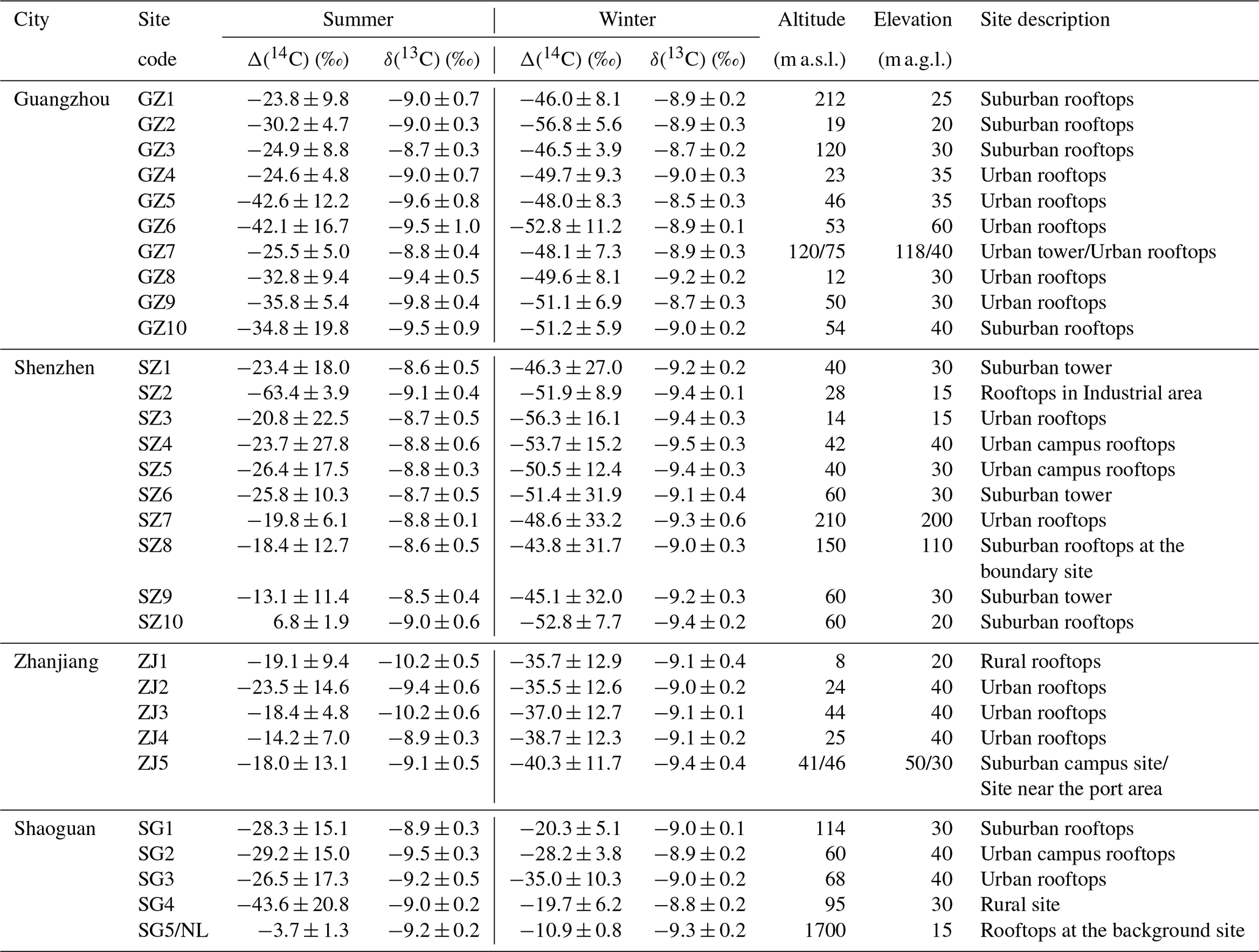
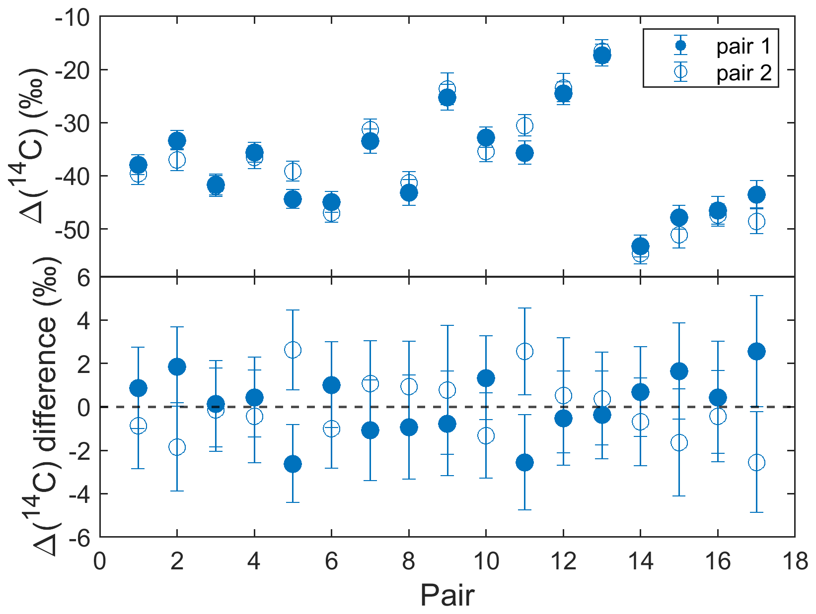
Figure A1 Pair differences of Δ(¹⁴C) for replicate measurements. Replicates were obtained from parallel air samples. The difference of each individual measurement from its pair mean is shown. Closed and open symbols are the first and second group taken from each pair, respectively. Error bars are the 1σ uncertainty on each measurement for the upper panel.

Appendix B: Radiocarbon isotope endmembers for biomass burning

Atmospheric ¹⁴CO₂ is assimilated by plants via photosynthesis, imprinting atmospheric Δ(¹⁴CO₂) signatures into plant tissues. This creates a bidirectional link: plant Δ(¹⁴C) reflects atmospheric Δ(¹⁴CO₂) levels, while atmospheric Δ(¹⁴CO₂) dynamics can be inferred from plant biomass archives (e.g., tree-ring). Annual biomass Δ(¹⁴C) closely matches contemporaneous atmospheric Δ(¹⁴CO₂) (due to rapid carbon turnover within a single growing season). Multi-year biomass Δ(¹⁴C) represents an integrated signal, blending atmospheric Δ(¹⁴CO₂) variations over its growth period (e.g., tree-ring capture annual Δ(¹⁴CO₂) fluctuations).

B1 Annual biomass

The Δ(¹⁴C) for annual biomass (Δ_a) in 2022 was estimated as $-\mathrm{14.8}\pm \mathrm{2.2}\mathrm{‰}$ (mean ± MSE), derived from a linear regression model of atmospheric Δ(¹⁴CO₂) decline ($-\mathrm{4.4}\mathrm{‰}{\mathrm{a}}^{-\mathrm{1}}$) observed in Northern Hemisphere zone 3 between 2010 and 2018 (Hua et al., 2022).

B2 Multi-year biomass

The Δ(¹⁴C) for multi-year biomass (Δ_m) is related with its age; the year it was growing, the annual increase in biomass, and atmospheric ¹⁴CO₂ during its growth cycle. The Δ(¹⁴C) for multi-year biomass can be determined (Lewis et al., 2004):

$$\begin{array}{}\text{(B1)}& \mathrm{\Delta }{}^{\mathrm{14}}{\mathrm{C}}_{\mathrm{m}}={\displaystyle \frac{{\int }_{t_{\mathrm{1}}}^{t_{\mathrm{2}}}\mathrm{\Delta }{}^{\mathrm{14}}\mathrm{C}\left(t\right)w\left(t\right)\mathrm{d}t}{{\int }_{t_{\mathrm{1}}}^{t_{\mathrm{2}}}w\left(t\right)\mathrm{d}t}}\end{array}$$

where Δ¹⁴C(t) is the atmospheric Δ(¹⁴CO₂) at age t, and the weighting function w(t) is the growth rate of carbon in biomass at age t, which can be determined by the Chapman–Richards growth model (Lewis et al., 2004):

$$\begin{array}{}\text{(B2)}& {\displaystyle }& {\displaystyle }V=A{\left(\mathrm{1}-{\mathrm{e}}^{-\frac{t-t_{\mathrm{0}}}{\mathit{\tau }}}\right)}^m\text{(B3)}& {\displaystyle }& {\displaystyle }w\left(t\right)={\displaystyle \frac{\mathrm{d}V}{\mathrm{d}t}}\end{array}$$

where V is the volume of a tree at age t (V=0 at t=t₀), and the parameters A, τ, and m can be chosen empirically to fit measured tree growth characteristics. The Chapman–Richards growth model describes cumulative growth of V.

It is assumed that the multi-year biomass was partitioned into five age cohorts (10, 20, 40, 65, and 85 year-old trees) with relative share of 20±10 %, 20±10 %, 40±20 %, 10±5 % and 10±5 %, respectively (Mohn et al., 2008). The corresponding Δ(¹⁴C) values were calculated as 20.9±5.4 ‰, 52.9±4.0 ‰, 137.5±35.1 ‰, 261.2±50.4 ‰, and 203.1±17.4 ‰, respectively. Consequently, the Δ(¹⁴C) signature of the multi-year biomass for the year 2022 was estimated as 116.2±17.6 ‰ (mean ±1σ; Δ_m) using the Chapman–Richards growth model (τ=50, m=3) and long-term tree-ring Δ(¹⁴C) measurements (Hua et al., 2022).

B3 Biomass burning

The Δ(¹⁴C) endmember for biomass burning (Δ_BB) was calculated using the two biomass types:

$$\begin{array}{}\text{(B4)}& {\mathrm{\Delta }}_{\text{BB}}=f_{\mathrm{a}}\times {\mathrm{\Delta }}_{\mathrm{a}}+(\mathrm{1}-f_{\mathrm{a}})\times {\mathrm{\Delta }}_{\mathrm{m}}\end{array}$$

where Δ_a and Δ_m represent the Δ(¹⁴C) signatures of annual biomass (e.g., crop residues) and multi-year biomass (e.g., woody waste), respectively, and f_a is the annual biomass fraction.

Using this framework, we estimated the 2022 Δ(¹⁴C) endmembers for biomass burning as 116.2±17.6 ‰, 103.1±15.8 ‰, 90.0±14.1 ‰, 76.9±12.3 ‰, 63.8±10.6 ‰, and 50.7±8.9 ‰ for f_a values of 0 %, 10 %, 20 %, 30 %, 40 %, 50 %, respectively.

Appendix C: Bias correction for C_ff calculation

C1 Air–sea exchange

The potential influence of CO₂ outgassing from the adjacent South China Sea (SCS) on our onshore measurements was assessed. Although the SCS is a net source of CO₂ to the atmosphere (with an annual flux of 0.44 $\mathrm{mol}{\mathrm{m}}^{-\mathrm{2}}{\mathrm{yr}}^{-\mathrm{1}}$; Li et al., 2020), its influence is negligible. This conclusion is supported by an analogous study of the California coast: the high-resolution WRF-STILT simulation by Graven et al. (2018) was conducted using flux data that included intense local nearshore sources (with fluxes up to 1.11 $\mathrm{mol}{\mathrm{m}}^{-\mathrm{2}}{\mathrm{yr}}^{-\mathrm{1}}$; Turi et al., 2014). Their results demonstrated that even these potent sources altered onshore CO₂ concentrations by less than 0.001 ppm (Graven et al., 2018). Given that the regional net flux from the SCS is weaker than this analogue, we conclude its impact on our Δ(¹⁴CO₂) measurements and derived C_ff estimates is physically insignificant and within the measurement uncertainty.

C2 Nuclear facilities

All operational (Daya Bay, Ling'ao, Yangjiang, Taishan) and under-construction (Lufeng, Taipingling, Lianjiang) nuclear power plants (NPPs) along the Guangdong Province coastline (Table C1) employ pressurized water reactor (PWR) technology. Airborne ¹⁴C releases from these facilities are predominantly hydrocarbons (75 %–95 %), mainly CH₄, with only a small fraction emitted as CO₂ (IAEA, 2004). In fact, almost all commercial reactors in China (>95 %) are of the PWR type, which exhibits the lowest ¹⁴CO₂ emission factor among nuclear technologies (Graven and Gruber, 2011; Yang, 2024).

Graven and Gruber (2011) reported that most of China and the western US are regions with minimal potential bias in ¹⁴CO₂-based C_ff estimates, owing to strong fossil fuel signals and limited nuclear ¹⁴C influence. Consistently, Graven et al. (2018) simulated the impact of reactor emissions on atmospheric Δ¹⁴CO₂ using WRF-STILT and found that an average ¹⁴CO₂ release rate of 6.6 Ci yr⁻¹ ($\sim \mathrm{0.24}\mathrm{TBq}{\mathrm{yr}}^{-\mathrm{1}}$) from the Diablo Canyon NPP in California produced an effect of <0.1 ppm in inferred C_ff at all sites, confirming that nuclear ¹⁴C emissions have a negligible influence on atmospheric radiocarbon measurements.

In Guangdong Province, Zazzeri et al. (2018) estimated ¹⁴CO₂ emissions from the Daya Bay, Ling'ao, and Yangjiang NPPs to be 0.111, 0.233, and 0.166 TBq yr⁻¹, respectively, values comparable to or smaller than those reported for Diablo Canyon. Although Daya Bay and Ling'ao are located only 6–7 km from the nearest observation site (SZ10) (Table C1), their emission rates remain extremely low. Under prevailing southeasterly winds in summer and northeasterly winds in winter, dispersion within the coastal boundary layer further dilutes any potential ¹⁴CO₂ plumes before they reach the sampling locations. Based on Gaussian plume scaling and regional wind climatology, we estimate that even under typical plume condition, the contribution of local reactor ¹⁴CO₂ to measured Δ¹⁴CO₂ at these urban sites would be <0.1 ‰, corresponding to an effect on inferred C_ff below 0.05 ppm. This estimate can be regarded as an upper bound for potential nuclear contamination at our sites, because all NPPs that could influence Guangzhou are located at distances>100 km from the Guangzhou observation site (Table C1).

Therefore, even for the closest stations, the impact of nearby nuclear facilities on Δ¹⁴CO₂ measurements is considered negligible and does not affect our radiocarbon-based source partitioning. For Guangzhou in particular, any nuclear influence on individual flask samples, and thus on the derived C_ff trend, is expected to be even smaller than this upper bound and negligible compared to other sources of uncertainty.

Table C1 Summary of operational nuclear facility in Guangdong Province: installed capacity, operational period, ¹⁴CO₂ emissions, and proximity to sampling sites with dominant wind directions.

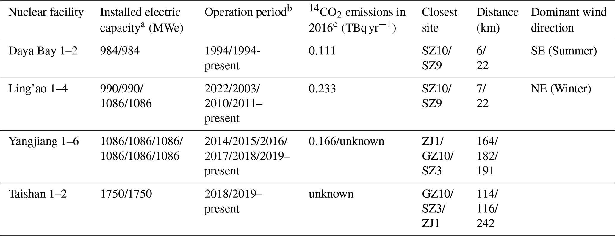
^a Data from China Nuclear Energy Association, Operational Performance of Nuclear Power in China (January–December 2024) (in Chinese). Retrieved from: https://www.china-nea.cn/site/content/48480.html (last access: 18 October 2025). ^b Data from National Nuclear Safety Administration, The Status of Mainland China's Nuclear Power Units in 2024 (in Chinese). Retrieved from: https://nnsa.mee.gov.cn/ywdt/hyzx/202501/t20250107_1100142.html (last access: 18 October 2025). ^c Emission data from Zazzeri et al. (2018), estimated using emission factors multiplied by IAEA PRIS data, assuming 28 % of ¹⁴C released from PWRs is in the form of CO₂.

C3 Biospheric exchange

Biospheric carbon fluxes associated with photosynthesis, autotrophic respiration, and annual biomass burning generally do not alter atmospheric Δ(¹⁴C) levels, as the carbon exchanged through these processes largely maintains isotopic equilibrium with contemporary atmospheric CO₂ (Turnbull et al., 2009). In contrast, heterotrophic respiration and multi-year biomass burning (e.g., wildfire consuming legacy organic matter) release carbon fixed during periods of elevated atmospheric Δ(¹⁴C), such as the 1960s nuclear bomb testing peak. This temporal decoupling between carbon uptake and release introduces a measurable positive bias in modern Δ(¹⁴C), reflecting the delayed contribution of older carbon pools. Therefore, we use estimates of heterotrophic respiration (Rh) and biomass burning (BB) fluxes to correct for biospheric influence on C_ff calculation.

C3.1 Heterotrophic respiration

The heterotrophic respiration correction term (β_Rh) is calculated by the following equation:

$$\begin{array}{}\text{(C1)}& {\mathit{\beta }}_{\text{Rh}}={\displaystyle \frac{C_{\mathrm{Rh}}({\mathrm{\Delta }}_{\text{bg}}-{\mathrm{\Delta }}_{\text{Rh}})}{{\mathrm{\Delta }}_{\text{bg}}+\mathrm{1000}\mathrm{‰}}}\end{array}$$

where C_Rh is the CO₂ mole fraction estimated by coupling hourly FLEXPART footprints with the heterotrophic respiration fluxes extracted from the Carnegie Ames Stanford Approach Global Fire Emissions Database Version 4 (CASA-GFED4s) (Randerson et al., 2017; Van Der Werf et al., 2017). We imposed the diurnal cycle from the CASA-GFED3 (Van Der Werf et al., 2010) heterotrophic respiration fluxes (estimated as half of the ecosystem respiration, which is calculated as the difference between net ecosystem exchange and gross ecosystem exchange; $[\text{NEE}-\text{GEE}]/\mathrm{2}$) onto the nearest neighbor CASA-GFED4s monthly mean fluxes to approximate hourly resolved fluxes. By aggregating these flux estimates, we created flux maps matching the spatial resolution of the hourly FLEXPART footprints. We then calculated C_Rh by multiplying the FLEXPART footprints with heterotrophic respiration flux maps. The simulated C_Rh concentrations were $\mathrm{1.5}\pm \mathrm{0.7}\mathrm{\mu }\mathrm{mol}{\mathrm{mol}}^{-\mathrm{1}}$ (range: $\mathrm{0.5}-\mathrm{3.1}\mathrm{\mu }\mathrm{mol}{\mathrm{mol}}^{-\mathrm{1}}$) in summer and $\mathrm{2.2}\pm \mathrm{0.9}\mathrm{\mu }\mathrm{mol}{\mathrm{mol}}^{-\mathrm{1}}$ (range: $\mathrm{0.4}-\mathrm{3.8}\mathrm{\mu }\mathrm{mol}{\mathrm{mol}}^{-\mathrm{1}}$) in winter.

We used a value of 40±35 ‰ for the Δ(¹⁴CO₂) signature of heterotrophic respiration (Δ_Rh), based on the value of 75±35 ‰ in 2015 (Graven et al., 2018) and considering a decrease of 5 ‰ per year (Zazzeri et al., 2023). The disequilibrium correction from heterotrophic respiration (β_Rh) were estimated to be $-\mathrm{0.06}\pm \mathrm{0.03}\mathrm{ppm}$ (range: −0.14 to −0.02 ppm) in summer and $-\mathrm{0.11}\pm \mathrm{0.04}\mathrm{ppm}$ (range: −0.20 to −0.02 ppm) in winter.

C3.2 Biomass burning

For the influence of biomass burning, we compared CO₂ emissions from two datasets: CASA-GFED4s (Randerson et al., 2017; Van Der Werf et al., 2017), and the Emissions Database for Global Atmospheric Research (EDGAR) (EDGAR, 2024). The key methodological distinction lies in their scopes. CASA-GFED4s quantifies emissions from open-environment fires that are detectable by satellites, including wildfires, agricultural residue burning, savanna/rangeland fires, and other small-scale open burning events. In contrast, EDGAR C_{bio_edgar} represents anthropogenic biofuel combustion, such as emissions from industrial and residential biomass use, while explicitly excluding large-scale wildfires and land-use change–related emissions (LULUCF). Thus, the two datasets characterize different aspects of biomass combustion: CASA-GFED4s captures open burning, whereas EDGAR focuses on controlled, human-induced combustion.

Across Guangdong Province and the four studied cities, biomass burning emissions from CASA-GFED4s accounted for <2 % of Rh emissions, indicating a minor contribution from open-environment fires in this region. By contrast, EDGARv2024ghg C_{bio_edgar} estimates represented a much larger proportion of Rh emissions, ranging from 7 %–29 % (Guangdong), 24 %–92 % (Guangzhou), 16 %–97 % (Shenzhen), 13 %–38 % (Zhanjiang), and 73 %–248 % (Shaoguan). Given the negligible magnitude of CASA-GFED4s emissions and their minimal effect on C_ff quantification, we focused on the EDGAR C_{bio_edgar} dataset for subsequent analysis. This dataset provides a more complete and representative estimate of anthropogenic biomass combustion CO₂ emissions in urban areas, which are most relevant to our study objectives.

To estimate the biomass burning correction term (β_BB) using the EDGAR2024 C_bio inventory (EDGAR, 2024), we first derived total C_BB simulations (C_BB) by applying a biomass burning fraction (α_BB) to the C_{bio_edgar} simulations (C_{bio_edgar}). This parameter α_BB represents the proportion of C_{bio_edgar} emissions attributable to biomass burning:

$$\begin{array}{}\text{(C2)}& C_{\mathrm{BB}}=C_{\text{bio\_edgar}}\times {\mathit{\alpha }}_{\text{BB}}\end{array}$$

The correction term β_BB was subsequently calculated as:

$$\begin{array}{}\text{(C3)}& {\mathit{\beta }}_{\text{BB}}={\displaystyle \frac{C_{\mathrm{BB}}({\mathrm{\Delta }}_{\text{bg}}-{\mathrm{\Delta }}_{\text{BB}})}{{\mathrm{\Delta }}_{\text{bg}}+\mathrm{1000}\mathrm{‰}}}\end{array}$$

For simulated C_{bio_edgar} mole fraction estimation in 2022, we implemented a three-stage process: (1) Generating 0.1°×0.1° resolution flux maps through integration of EDGAR2024 C_{bio_edgar} emission fluxes with FLEXPART atmospheric transport footprints, (2) performing spatiotemporal aggregation to align with FLEXPART model output specifications, and (3) calculating concentrations via convolution operations between transport footprints and optimized flux fields.

We adopted Δ(¹⁴CO₂) signatures of $-\mathrm{14.8}\pm \mathrm{2.2}\mathrm{‰}$ (annual biomass burning) and 116.2±17.6 ‰ (multi-year biomass burning) calculated in Appendix B. For 2022 Δ(¹⁴C) endmembers for biomass burning, we estimated values of 116.2±17.6 ‰ (0 % annual biomass), 103.1±15.8 ‰ (10 %), 90.0±14.1 ‰ (20 %), 76.9±12.3 ‰ (30 %), 63.8±10.6 ‰ (40 %), and 50.7±8.9 ‰ (50 %), corresponding to incremental annual biomass burning fractions from 0 % to 50 %.

We quantified disequilibrium correction terms under the maximum biomass burning (BB) contribution scenario (f_a=0 % and α_BB=100 %). The simulated C_BB concentrations were $\mathrm{0.8}\pm \mathrm{0.7}\mathrm{\mu }\mathrm{mol}{\mathrm{mol}}^{-\mathrm{1}}$ (range: $\mathrm{0.0}-\mathrm{1.9}\mathrm{\mu }\mathrm{mol}{\mathrm{mol}}^{-\mathrm{1}}$) in summer and $\mathrm{1.9}\pm \mathrm{1.0}\mathrm{\mu }\mathrm{mol}{\mathrm{mol}}^{-\mathrm{1}}$ (range: $\mathrm{0.1}-\mathrm{4.4}\mathrm{\mu }\mathrm{mol}{\mathrm{mol}}^{-\mathrm{1}}$) in winter. The BB-specific correction term (β_BB) exhibited seasonal variations: $-\mathrm{0.09}\pm \mathrm{0.08}\mathrm{\mu }\mathrm{mol}{\mathrm{mol}}^{-\mathrm{1}}$ (range: −0.46 to $-\mathrm{0.01}\mathrm{\mu }\mathrm{mol}{\mathrm{mol}}^{-\mathrm{1}}$) in summer and $-\mathrm{0.24}\pm \mathrm{0.12}\mathrm{\mu }\mathrm{mol}{\mathrm{mol}}^{-\mathrm{1}}$ (range: −0.56 to $-\mathrm{0.02}\mathrm{\mu }\mathrm{mol}{\mathrm{mol}}^{-\mathrm{1}}$) in winter under 0 % annual biomass burning contribution. The combined correction factor β, integrating contributions from both heterotrophic respiration (Rh) and biomass burning (BB), showed broader ranges: $-\mathrm{0.16}\pm \mathrm{0.09}\mathrm{\mu }\mathrm{mol}{\mathrm{mol}}^{-\mathrm{1}}$ (range: −0.55 to $-\mathrm{0.03}\mathrm{\mu }\mathrm{mol}{\mathrm{mol}}^{-\mathrm{1}}$) in summer and $-\mathrm{0.35}\pm \mathrm{0.15}\mathrm{\mu }\mathrm{mol}{\mathrm{mol}}^{-\mathrm{1}}$ (range: −0.72 to $-\mathrm{0.04}\mathrm{\mu }\mathrm{mol}{\mathrm{mol}}^{-\mathrm{1}}$) in winter.

Appendix D: Background selection

As we summarized in Zhou et al. (2024), Turnbull et al. (2015) concluded that for Indianapolis, a city with relatively simple boundary conditions, the upwind background site (Tower 1) is more appropriate compared with continental and regional background sites (LEF and NWR). In contrast, for Los Angeles, a city with relatively complex boundary conditions, Newman et al. (2016) and Miller et al. (2020) tend to use the neighboring regional or continental background sites (MWO and LJO; BRW and NWR), because the upwind background within the city may be influenced by emissions from neighboring cities and therefore cannot represent the local urban background.

In this study, the cities concerned are central cities or neighboring cities of the Pearl River Delta (PRD) urban agglomeration with relatively complex boundary conditions, so we chose the nearest regional background site NL (i.e., SG5) as the background for determining the C_ff concentrations.

The Nanling site serves as an ideal atmospheric background monitoring station for Guangdong due to its remote location (>100 km from the PRD urban agglomeration), high-altitude terrain (1700 m a.s.l.) avoiding localized pollution. Situated above the mixed boundary layer under most meteorological conditions, NL is well isolated from urban influences. Its strategic position as a climatic and watershed boundary intercepting seasonal airflows further enables precise monitoring of regional atmospheric transport patterns while meeting strict background-station criteria for pollution isolation and cross-boundary impact assessment.

In addition, trajectory and potential source region analyses further confirm that the Nanling site is representative of regional background air under both monsoon regimes. HYSPLIT clustering and PSCF analyses by Zhang et al. (2022) showed that during winter, air masses arriving at Nanling predominantly originate from the northern inland provinces (e.g., Hunan, Jiangxi, Sichuan), while in summer they mostly come from the South China Sea and southeastern coastal regions. These summer air masses are typically marine-influenced and low in CO₂, consistent with clean background characteristics.

Continuous CO observations at NL further support its background representativeness: approximately 90 % of summer samples had concentrations below 200 ppb, comparable to other regional background sites, indicating that pollution from the PRD rarely reaches NL. Therefore, NL can be considered a robust regional background site for both monsoon seasons.

Furthermore, the “annual” CO₂ and Δ(¹⁴C) averages at NL, which are close to those at the Jungfraujoch, occupy the upper-right section of the Keeling plot of Δ(¹⁴C) versus CO₂, representing the background end-member when compared with Waliguan (Fig. 3). Additionally, the Δ(¹⁴C) and CO₂ averages at NL were the highest and the lowest, respectively, among the 30 sampling sites (Table A1), consistent with background-level characteristics.

Appendix E: Comparison of C_ff fractions and concentrations among various cities

Table E1 Comparison of C_ff and C_bio fractions derived from Δ(¹⁴CO₂) measurements in various cities.

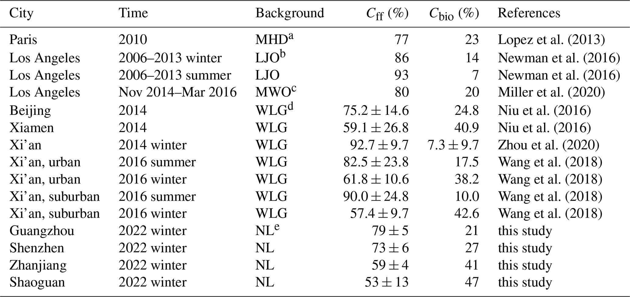
^a Mace Head, ^b La Jolla, ^c Mount Wilson Observatory, ^d Waliguan, ^e Nanling.

Table E2 Comparison of C_ff concentrations derived from Δ(¹⁴CO₂) measurements in various cities.

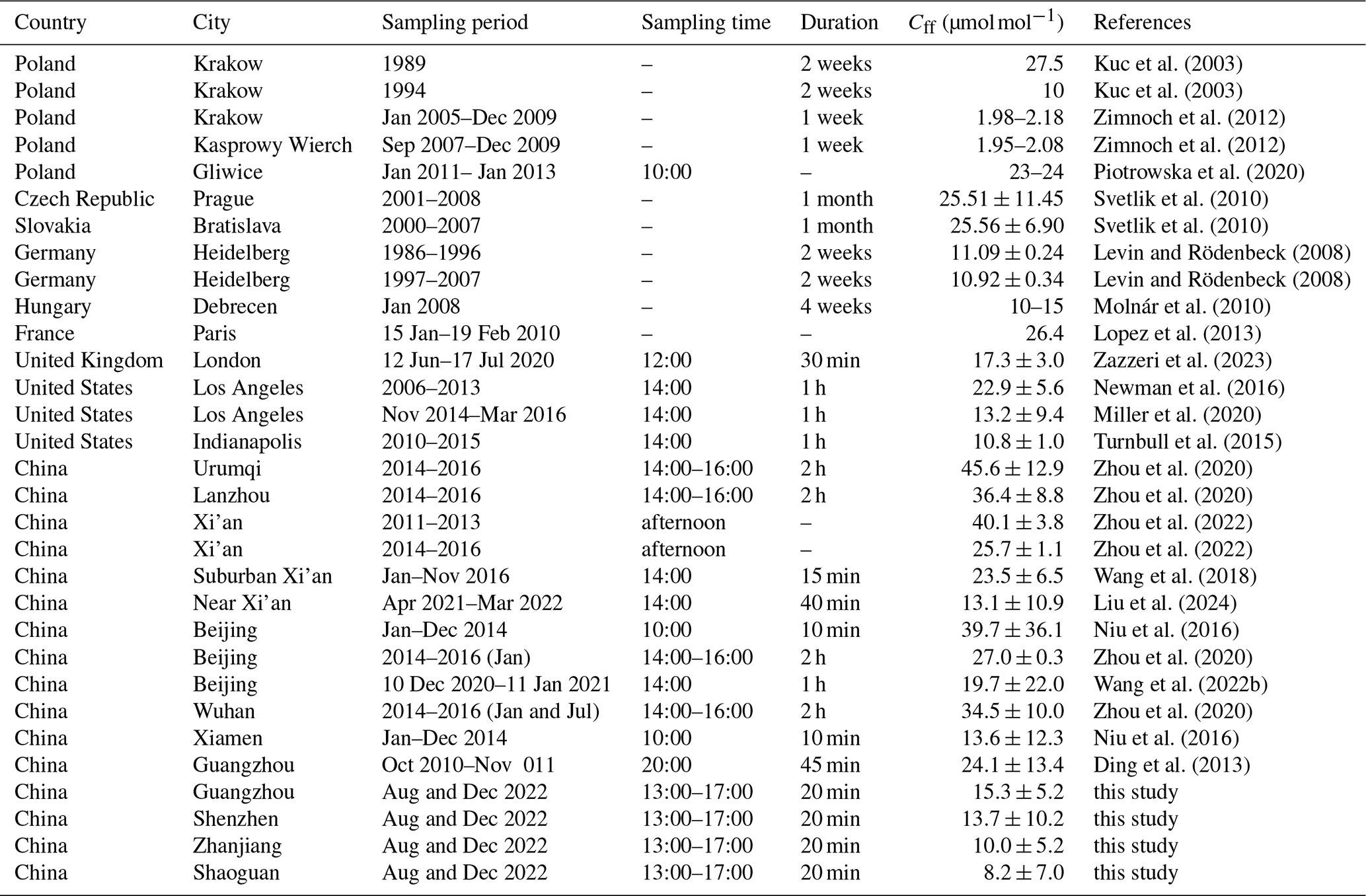
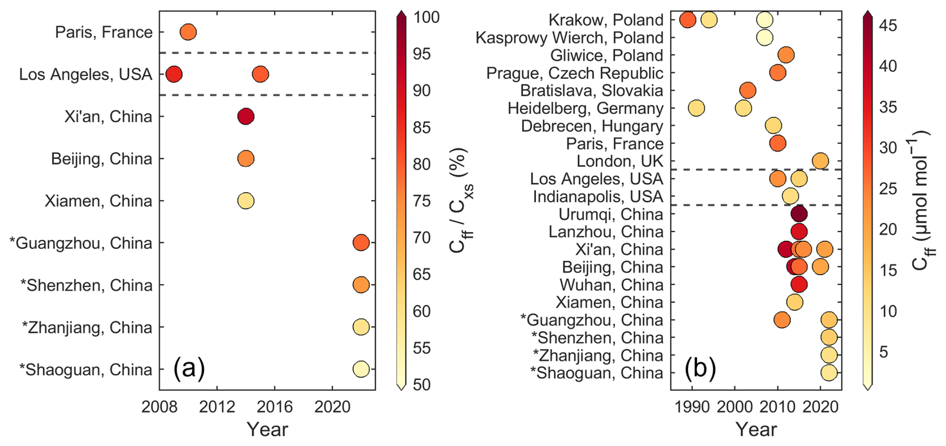
Figure E1 Comparison of (a) C_ff fractions in C_xs and (b) C_ff concentrations derived from Δ(¹⁴CO₂) measurements from previous studies and this study (^∗) in various cities across European countries (Kuc et al., 2003; Levin and Rödenbeck, 2008; Molnár et al., 2010; Svetlik et al., 2010; Zimnoch et al., 2012; Lopez et al., 2013; Piotrowska et al., 2020; Zazzeri et al., 2023), United States (Turnbull et al., 2015; Newman et al., 2016; Miller et al., 2020), and China (Ding et al., 2013; Niu et al., 2016; Zhou et al., 2020; Wang et al., 2022b; Liu et al., 2024; Zhou et al., 2022). In (a), Los Angeles, Beijing, Guangzhou, and Shenzhen are megacities, Xi'an is a supercity, and other are large and medium cities (China Population Census by County Council et al., 2022). Values in (a, b) refer to Tables E1 and E2, respectively.

Appendix F: HYSPLIT back trajectories and FLEXPART footprints

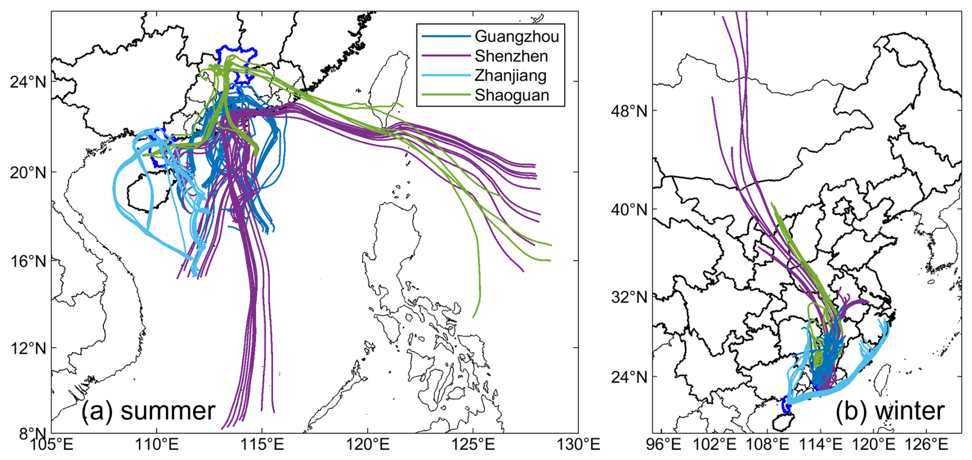
Figure F1 HYSPLIT back trajectories for a 72 h duration for Guangzhou, Shenzhen, Zhanjiang, and Shaoguan in (a) summer and (b) winter. The trajectories reveal maritime inflow in summer and continental inflow in winter, corroborating the ERA5-based analysis. National boundaries were taken from Natural Earth (https://www.naturalearthdata.com/, last access: 9 March 2024).

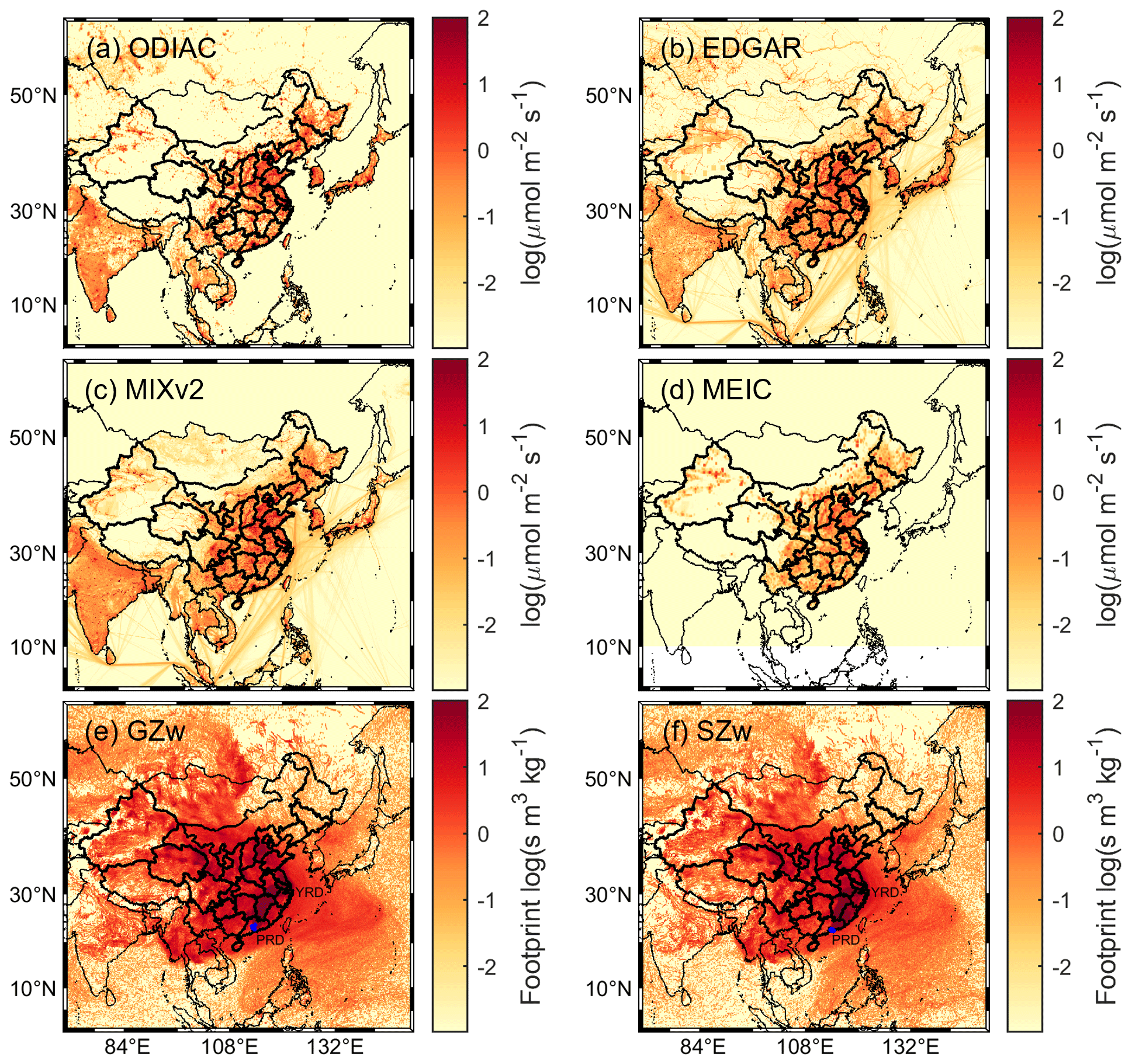
Figure F2 Annual mean C_ff emissions in China from four gridded inventory datasets: (a) ODIAC, (b) EDGAR, (c) MIXv2, and (d) MEIC, and FLEXPART footprints simulating C_ff emissions for (e) Guangzhou (GZ), (f) Shenzhen (SZ) in winter (w) by releasing particles at the blue sampling sites at heights from 0–100 m a.s.l. over a period of 30 d. The YRD and PRD represent Yangtze River Delta and Pearl River Delta urban agglomeration labelled in (e, f). Boundaries of nations and Chinese provinces were obtained from Natural Earth (https://www.naturalearthdata.com/, last access: 9 March 2024).

Appendix G: Transport representativeness analysis

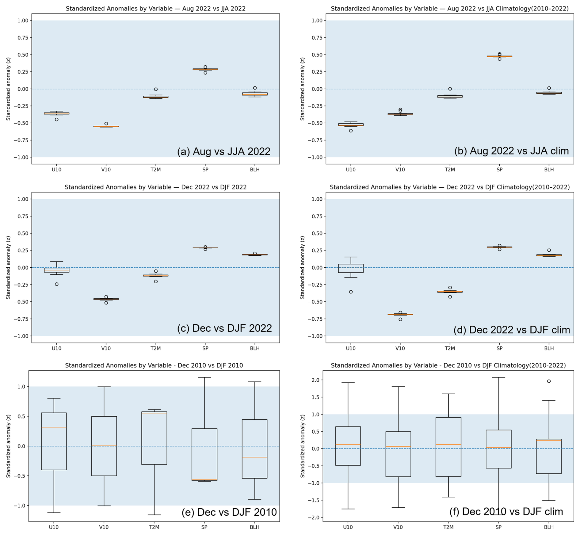
Figure G1 Box-and-whisker plots of standardized anomalies (z) by ERA5 meteorological variables (U10, V10, T2M, SP, BLH) for (a) August 2022 vs. JJA 2022, (b) August 2022 vs. JJA climatology (2010–2022), (c) December 2022 vs. DJF 2022, and (d) December 2022 vs. DJF climatology (2010–2022) across Guangzhou sites (GZ1-10), and (e) December 2010 vs. DJF 2010, and (f) December 2010 vs. DJF climatology (2010–2022) at GZ7. U10, V10, T2M, SP, BLH are 10 m zonal and meridional winds (U10, V10), 2 m temperature (T2M), surface pressure (SP), and planetary boundary-layer height (PBLH), respectively. The shaded region denotes $\left|z\right|\le \mathrm{1}$ (typical range).

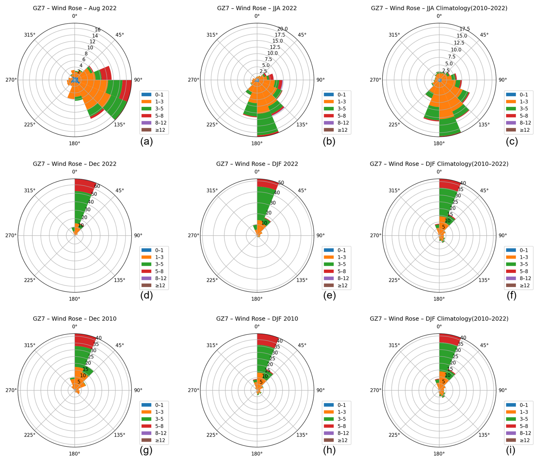
Figure G2 ERA5 wind roses for GZ7 site (wind speed unit: m s⁻¹) showing six panels: (a) August 2022, (b) JJA 2022, (c) JJA climatology (2010–2022), (d) December 2022, (e) DJF 2022, (f) DJF climatology (2010–2022), (g) December 2010, (h) DJF 2010, (i) DJF climatology (2010–2022). These illustrate that August 2022, December 2022, and December 2010 are consistent with their canonical summer and winter flow regimes.

Table G1 December 2010 vs. December 2022 statistics of U10, V10, wind speed, T2M, PBLH, and ventilation at GZ7, including mean, standard deviation, median, and p-values from Student's t-test and Mann–Whitney U test.

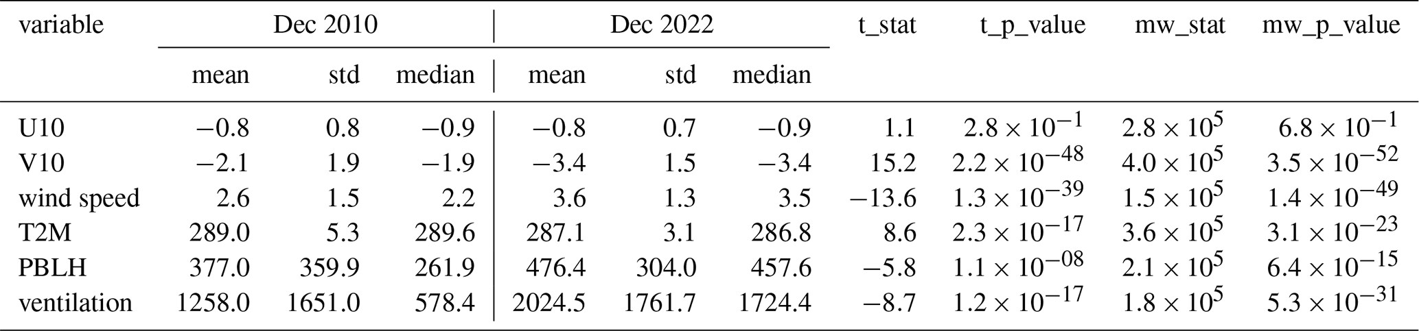
Table G2 December 2010 vs. December 2022 wind direction sector frequencies (in %) at GZ7.

Appendix H: Historical comparison and corrections

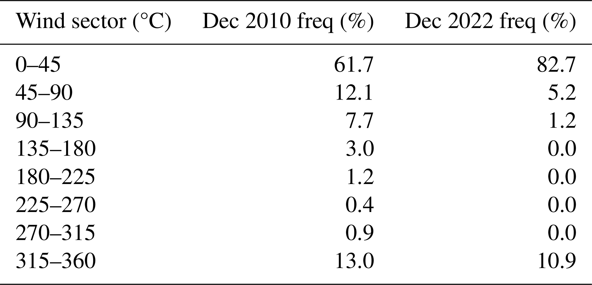
Table H1 Summary of all available C_ff datasets for historical variations used in this study and referenced from previous literature, including site type, coordinates, sampling period, time, number of samples (n), and references.

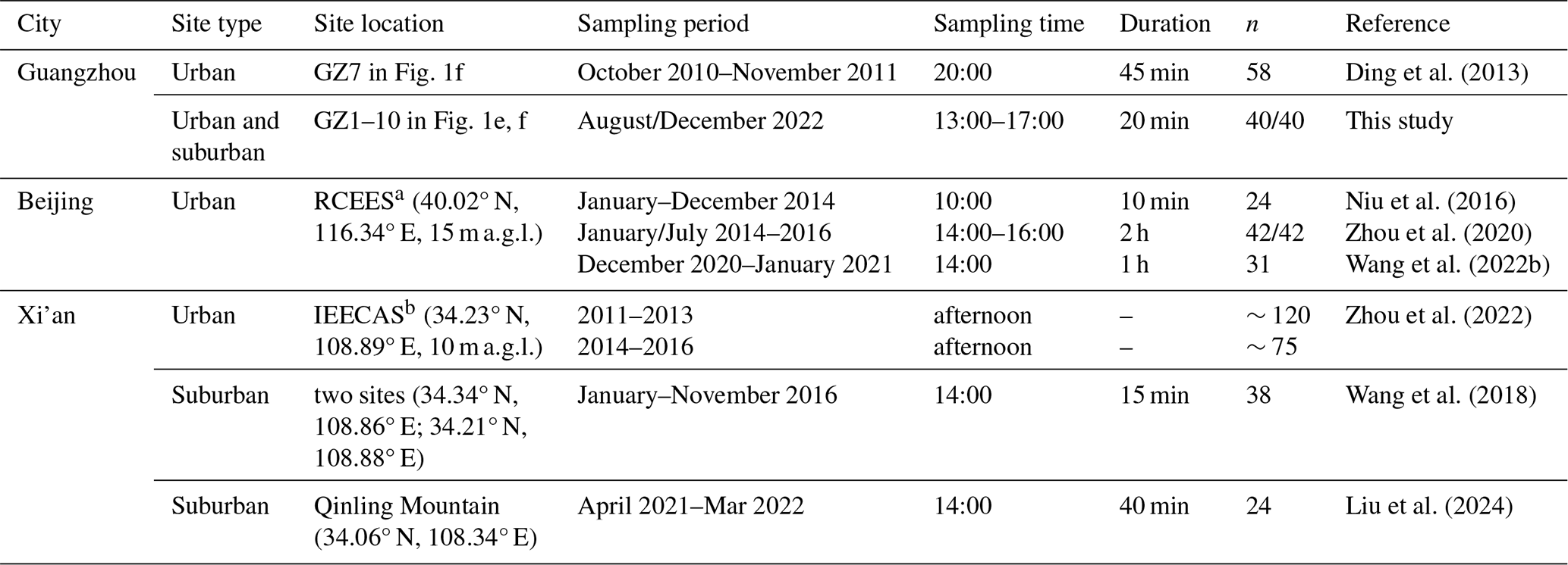
^a Research Center for Eco-Environmental Sciences, Chinese Academy of Sciences (RCEES). ^b Institute of Earth Environment, Chinese Academy of Sciences (IEECAS).

Table H2 Harmonized comparison of C_ff mole fractions at identical sites, seasons, and sampling times, after correction to common background conditions.

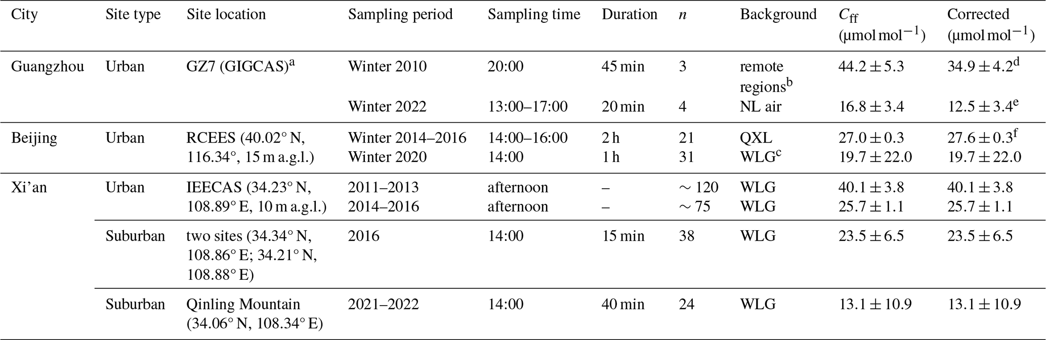
^a Guangzhou Institute of Geochemistry, Chinese Academy of Sciences (GIGCAS). ^b remote regions (Qinghai, Gansu, and Tibet) with Δ(¹⁴C) value of 37.5±3.0 ‰. ^c C_ff concentrations in winter Beijing obtained from Wang et al. (2022b) were estimated based on the background atmospheric Δ(¹⁴CO₂) measurements from Waliguan (Liu et al., 2024). ^d corrected to 14:00 sampling and recalculated using a common NL tree-ring Δ(¹⁴C) background as a harmonized reference baseline for inter-period comparison. The NL tree-ring Δ(¹⁴C) represents a growing-season (March–October) integrated proxy at Nanling, and the 2022 value (−20.8 ‰) is linearly extrapolated from the 2011–2020 tree-ring record (Li et al., 2025b); it is therefore not intended to represent wintertime background variability. ^e recalculated using the same NL tree-ring Δ(¹⁴C) harmonized reference baseline (33.9 ‰) as in footnote d. ^f corrected to the WLG background.

H1 Sampling-time difference (20:00 vs. 14:00) in C_ff for Guangzhou

Ding et al. (2013) collected flask samples around 20:00 LT, immediately after the evening rush hour, whereas our 2022 samples were collected between 13:00 and 17:00 LT under well-mixed boundary-layer conditions. To quantify the potential diurnal C_ff bias, we used continuous CO observations near GZ7 from two independent sources: (1) the Guangdong Provincial Environmental Monitoring Centre and (2) the nationwide air quality database (https://quotsoft.net/air/#messy, last access: 18 October 2025), and applied the formulation

$$\begin{array}{}\text{(H1)}& C_{\text{ff}}\approx \mathrm{\Delta }\mathrm{CO}/R\end{array}$$

where $\mathrm{\Delta }\mathrm{CO}=\mathrm{CO}-{\mathrm{CO}}_{\text{bg}}$, and $R=\mathrm{\Delta }\mathrm{CO}/\mathrm{\Delta }{\mathrm{CO}}_{\mathrm{2},\mathrm{ff}}$ denotes the concentration ratio between CO and fossil-fuel CO₂. The value of R is strongly time-dependent and source-specific. Nighttime R values tend to be higher than daytime values because (i) nighttime emissions are dominated by direct fossil-fuel combustion while biogenic CO₂ sources (e.g., respiration) remain constant but emit no CO, and (ii) oxidative sinks (e.g., OH radicals) are weaker at night. Therefore, applying an afternoon-derived R to nighttime data likely provides a lower bound for the actual nighttime C_ff enhancement.

Scheme 1 (this study's observation, December 2022)

We used the December diurnal mean CO data at a site close to GZ7, subtracted the NL background to obtain ΔCO, and divided by the afternoon-specific $R=\mathrm{13.3}\mathrm{ppb}{\mathrm{ppm}}^{-\mathrm{1}}$ (derived from the regression between ΔCO and ¹⁴C-based ΔCO_2,ff). The ΔCO increased from 168.3 ppb at 14:00 to 220.7 ppb at 20:00, corresponding to an estimated nighttime C_ff enhancement of approximately 3.2 ppm, or about 21 % higher than the afternoon value. Because the slope R was determined during well-mixed afternoon periods, this result likely represents a lower limit; the actual nighttime–afternoon C_ff contrast may be smaller.

Scheme 2 (Guangzhou dataset, winter 2023, supplementary analysis)

We applied the same approach to the continuous CO data at the site close to GZ7 for the winter season (December 2023 –February 2024). After subtracting the NL background, ΔCO was divided by the seasonal $R=\mathrm{9.08}\mathrm{ppb}{\mathrm{ppm}}^{-\mathrm{1}}$ obtained from regressions of CO against total CO₂ (Zhang et al., 2026). As this R reflects bulk CO₂ rather than specifically fossil-fuel CO₂, we applied an empirical correction (dividing R by 0.8; Turnbull et al., 2011). The resulting analysis indicates that ΔCO increased by 66.9 ppb from 14:00–20:00, implying a C_ff enhancement difference of roughly 5.9 ppm (≈35 %).

Overall, while continuous CO_2ff data are not available for 2022, our CO-based analysis suggests that the C_ff signal at 20:00 is moderately higher than that at 14:00. This finding is consistent with the reviewer's expectation that post–rush-hour conditions retain a stronger fossil-fuel signature compared with the well-mixed afternoon atmosphere. The semi-quantitative assessment indicates that the C_ff concentration during post–rush-hour (20:00) is approximately 21 %–35 % higher than during well-mixed afternoon periods, consistent with the expected diurnal accumulation of fossil-fuel CO₂ under weaker nighttime boundary-layer mixing.

Appendix I: Comparison of contributions of coal, oil and natural gas to C_ff concentrations in various cities

Table I1 Comparison of contributions of coal, oil and natural gas to C_ff concentrations in various cities.

Appendix J: $R_{\mathrm{CO}/{\mathrm{CO}}_{\mathrm{2}\mathrm{ff}}}$ for sites, cities and comparison

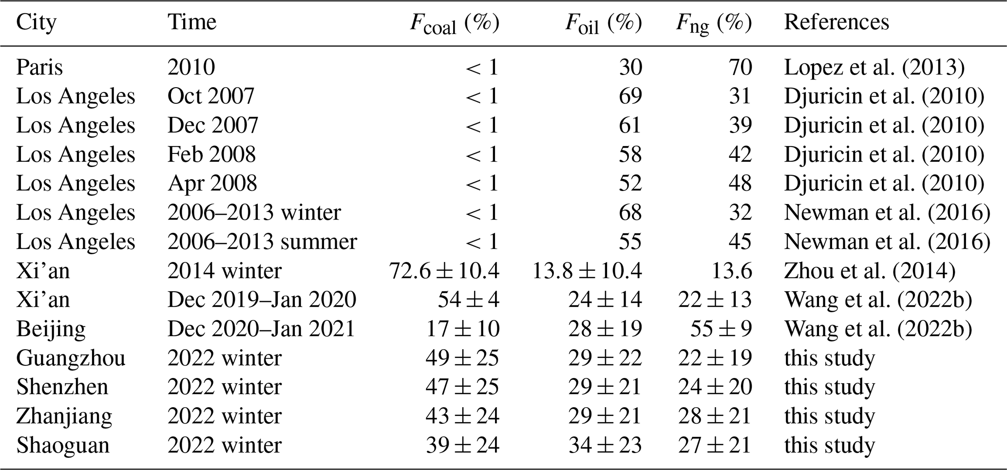
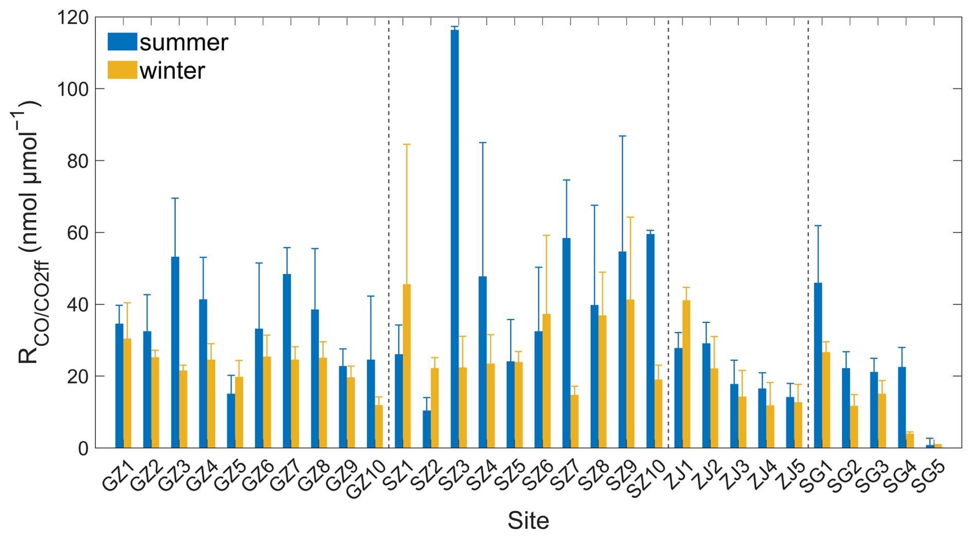
Figure J1 $R_{\mathrm{CO}/{\mathrm{CO}}_{\mathrm{2}\mathrm{ff}}}$ averages at the 30 sampling sites. Error bars denote ±1 SD of the seasonal $R_{\mathrm{CO}/{\mathrm{CO}}_{\mathrm{2}\mathrm{ff}}}$ ratios at each site.

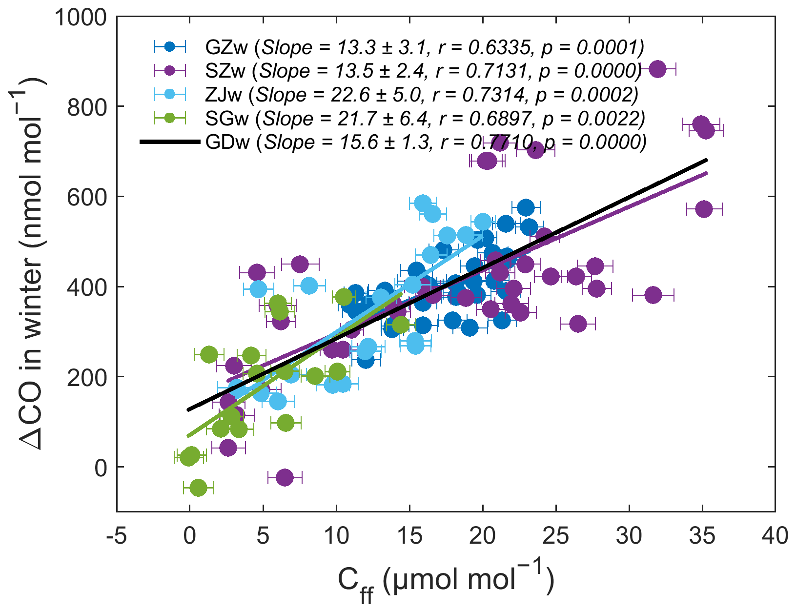
Figure J2 ΔCO : C_ff for Guangzhou, Shenzhen, Zhanjiang, and Shaoguan in winter. Vertical and horizontal error bars denote the propagated uncertainties in C_ff and CO, respectively, propagated from their measurement and calculation uncertainties.

Table J1 Observational concentration ratios of CO to C_ff ($R_{\mathrm{CO}/{\mathrm{CO}}_{\mathrm{2}\mathrm{ff}}}$) for China and Chinese cities.

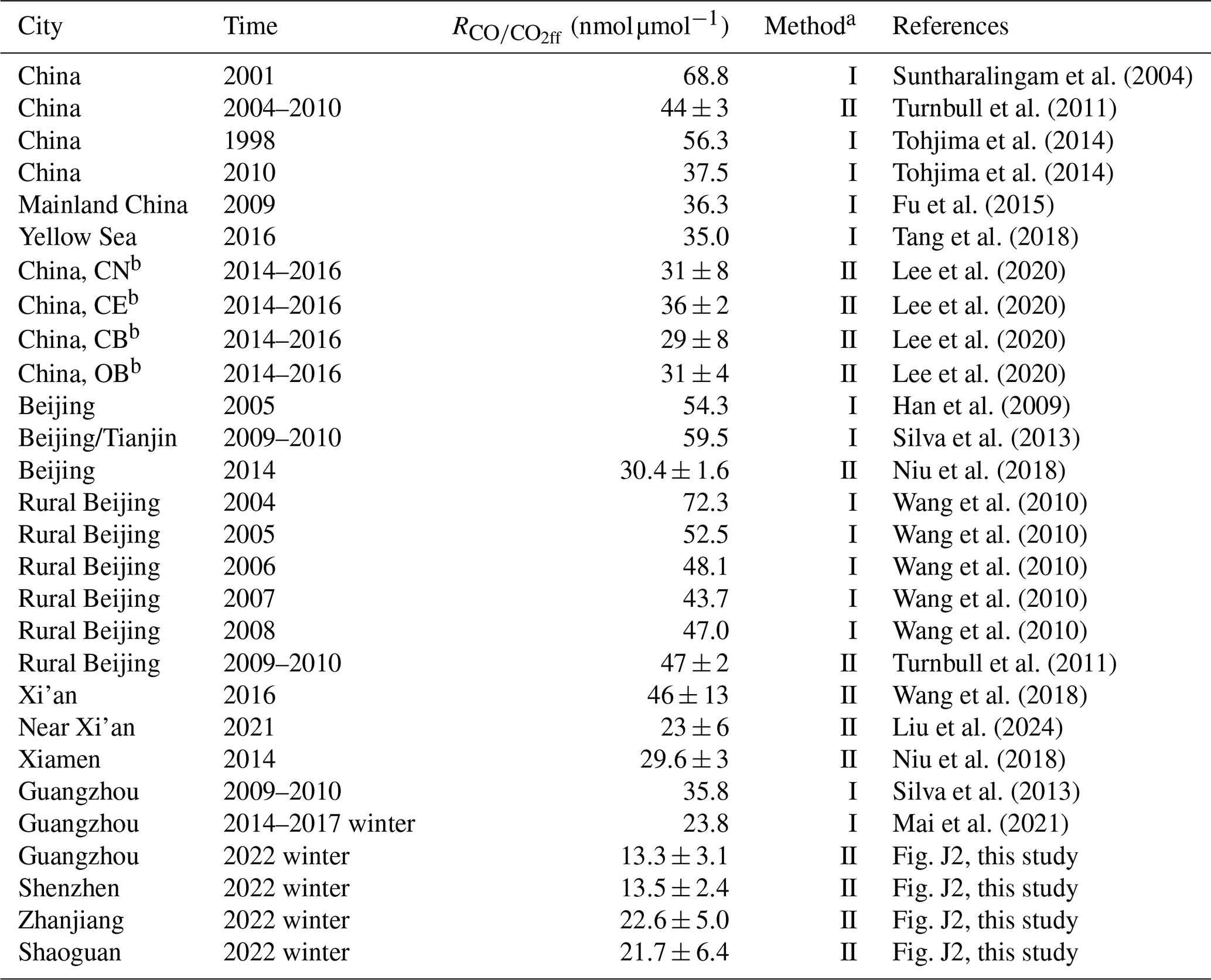
^a by correction from $R_{\mathrm{CO}/{\mathrm{CO}}_{\mathrm{2}}}$ by increased 20 % (Method I) and estimation from Δ(¹⁴C) measurements (Method II), ^b CN represents the air masses from northeast China, CE for central eastern China around the Shandong area, CB for continental background air, and OB for ocean background.